RoPINN: Region Optimized
Physics-Informed Neural Networks

Abstract

Physics-informed neural networks (PINNs) have been widely applied to solve partial differential equations (PDEs) by enforcing outputs and gradients of deep models to satisfy target equations. Due to the limitation of numerical computation, PINNs are conventionally optimized on finite selected points. However, since PDEs are usually defined on continuous domains, solely optimizing models on scattered points may be insufficient to obtain an accurate solution for the whole domain. To mitigate this inherent deficiency of the default scatter-point optimization, this paper proposes and theoretically studies a new training paradigm as region optimization. Concretely, we propose to extend the optimization process of PINNs from isolated points to their continuous neighborhood regions, which can theoretically decrease the generalization error, especially for hidden high-order constraints of PDEs. A practical training algorithm, Region Optimized PINN (RoPINN), is seamlessly derived from this new paradigm, which is implemented by a straightforward but effective Monte Carlo sampling method. By calibrating the sampling process into trust regions, RoPINN finely balances sampling efficiency and generalization error. Experimentally, RoPINN consistently boosts the performance of diverse PINNs on a wide range of PDEs without extra backpropagation or gradient calculation.

1 Introduction

Solving partial differential equations (PDEs) is the key problem in extensive areas, covering both engineering and scientific research [35, 37, 44]. Due to the inherent complexity of PDEs, they usually cannot be solved analytically [10]. Thus, a series of numerical methods have been widely explored, such as spectral methods [21, 37] or finite element methods [5, 7]. However, these numerical methods usually suffer from huge computational costs and can only obtain an approximate solution on discretized meshes [24, 40]. Given the impressive nonlinear modeling capability of deep models [4, 14], they have also been applied to solve PDEs, where physics-informed neural networks (PINNs) are proposed and have emerged as a promising and effective surrogate tool for numerical methods [41, 33, 32]. By formalizing PDE constraints (i.e. equations, initial and boundary conditions) as objective functions, the outputs and gradients of PINNs will be optimized to satisfy a certain PDE during training [33], which successfully instantiates the PDE solution as a deep model.

Although deep models have been proven with universal approximation capability, the actual optimization process of PINNs still faces thorny challenges [8, 22, 32]. As a basic topic of PINNs, the optimization problem has been widely explored from various aspects [16, 41]. Previous methods attempt to mitigate this problem by using novel architectures to enhance model capacity [53, 3, 45], reweighting multiple loss functions for more balanced convergence [42], resampling data to improve important areas [46] or developing new optimizers to tackle the rough loss landscape [50, 34], etc.

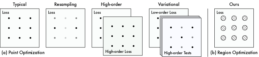
Figure 1: Comparison between previous methods and ours. Previous point optimization methods train PINNs via the loss on selected points, which is different from our region optimization paradigm.

Orthogonal to the above-mentioned methods, this paper focuses on a foundational problem, which is the objective function of PINNs. We notice that, due to the limitation of numerical calculation, it is almost impossible to optimize the loss function in the complete continuous domain. Thus, the conventional PINN loss is only defined on a series of selected points [33] (Figure 1). However, the scatter-point loss function obviously mismatches the PDE-solving objective, which is approximating the solution on a continuous domain. This mismatch may fundamentally limit the performance of PINNs. Several prior works also try to improve the canonical PINN loss function, which can be roughly categorized into the following two paradigms. One paradigm enhances the optimization by adding high-order derivatives of PDEs as a regularization term to the loss function [50]. However, calculating high-order gradients is numerically unstable and time-consuming, even with automatic differentiation in well-established deep learning frameworks [2, 31]. The other paradigm attempts to bypass the high-order derivative calculation in the PINN loss function with variational formulations [17, 18, 19]. Nevertheless, these variational methods still face difficulties in calculating the integral of deep models and will bring extra computations, thereby mainly limited to very shallow models or relying on massive sampled quadrature points and elaborative test functions [11, 52].

This paper proposes and studies a new training paradigm for PINNs as region optimization. As shown in Figure 1, we extend the optimization process from selected scatter points into their neighborhood regions, which can theoretically decrease the generalization error on the whole domain, especially for hidden high-order constraints of PDEs. In practice, we seamlessly transform this paradigm into a practical training algorithm, named Region Optimized PINN (RoPINN), which is implemented through simple but effective Monte Carlo sampling. In addition, to control the estimation error, we adaptively adjust the sampling region size according to the gradient variance among successive training iterations, which can constrain the sampling-based optimization into a neighborhood with low-variance loss gradients, namely trust region. In experiments, RoPINN demonstrates consistent and sharp improvement for diverse PINN backbones on extensive PDEs (19 different tasks) without any extra gradient calculation. Our contributions are summarized as follows:

• To mitigate the inherent deficiency of conventional PINN optimization, we propose the region optimization paradigm, which extends the scatter-point optimization to neighborhood regions that theoretically benefits both generalization and high-order constraints satisfaction.

• We present RoPINN for PINN training based on Monte Carlo sampling, which can effectively accomplish the region optimization. A trust region calibration strategy is proposed to reduce the gradient estimation error caused by sampling for more trustworthy optimization.

• RoPINN can consistently improve the performance of various PINN backbones (i.e. canonical and Transformer-based) on a wide range of PDEs without extra gradient calculation.

2 Preliminaries

A PDE with equation constraints, initial (ICs) and boundary conditions (BCs) can be formalized as

$$\mathcal{F}(u)(\boldsymbol{x})=0,\boldsymbol{x}\in\Omega;\ \mathcal{I}(u)(\boldsymbol{x})=0,\boldsymbol{x}\in\Omega_{0};\ \mathcal{B}(u)(\boldsymbol{x})=0,\boldsymbol{x}\in\partial\Omega,$$ (1)

where $\mathcal{F},\mathcal{I},\mathcal{B}$ denote the PDE equations, ICs and BCs respectively [6]. $u:\mathbb{R}^{d+1}\to\mathbb{R}^{m}$ is the target PDE solution. $\boldsymbol{x}\in\Omega\subseteq\mathbb{R}^{d+1}$ represents the input coordinate, which is usually a composition of spatial and temporal positions, namely $\boldsymbol{x}=(x_{1},\cdots,x_{d},t)$. $\Omega_{0}$ corresponds to the $t=0$ situation.

Correspondingly, the PINN loss function (point optimization) is typically defined as follows [16, 33]:

$$\begin{split}\mathcal{L}(u_{\theta})=&\frac{\lambda_{\Omega}}{N_{\Omega}}\sum_{{i=1}}^{N_{\Omega}}\|\mathcal{F}(u_{\theta})(\boldsymbol{x}_{{i}})\|^{2}+\frac{\lambda_{\Omega_{0}}}{N_{\Omega_{0}}}\sum_{{i=1}}^{N_{\Omega_{0}}}\|\mathcal{I}(u_{\theta})(\boldsymbol{x}_{{i}})\|^{2}+\frac{\lambda_{\partial\Omega}}{N_{\partial\Omega}}\sum_{{i=1}}^{N_{\partial\Omega}}\|\mathcal{B}(u_{\theta})(\boldsymbol{x}_{{i}})\|^{2},\end{split}$$ (2)

where $u_{\theta}$ represents the neural network parameterized by $\theta$. $N_{\Omega},N_{\Omega_{0}},N_{\partial\Omega}$ are the numbers of sampled points in $\Omega,\Omega_{0},\partial\Omega$ respectively. $\lambda_{\ast}$ is the corresponding loss weight. Note that there is an additional data loss term in Eq. (2) when we can access the ground truth of some points [33]. Since we mainly focus on PDE constraints throughout this paper, we omit the data loss term in the above formalization, which is still maintained in our experiments. In this paper, we try to improve PINN solving by defining a new surrogate loss in place of the canonical definition of PINN loss in Eq. (2). In contrast, the relevant literature mainly improves the objective function in two different directions as follows. Appendix F provides a more comprehensive discussion on other relative topics.

High-order regularization

The first direction is to add the high-order constraints of PDEs as regularization terms to the loss function [50]. Specifically, since PDEs are sets of identical relations, suppose that the solution $u$ is a $K$-order differential function, Eq. (1) can naturally derive a branch of high-order equations, where the $k$-th derivative for the $j$-th dimension is $\frac{\partial^{k}}{\partial x_{j}^{k}}\mathcal{F}(u)(\boldsymbol{x})=0,$ $\boldsymbol{x}\in\Omega,1\leq j\leq(d+1),1\leq k\leq K$, corresponding to the following regularization:

$$\begin{split}\mathcal{L}^{\mathrm{reg}}_{k,j}(u_{\theta})=\frac{\lambda_{k,j}}{N_{k,j}}\sum_{{i=1}}^{N_{k,j}}\left\|\frac{\partial^{k}}{\partial x_{j}^{k}}\mathcal{F}(u_{\theta})(\boldsymbol{x}_{{i}})\right\|^{2},\end{split}$$ (3)

where $N_{k,j}$ denotes the number of sampled points with weight $\lambda_{k,j}$. Although this design can explicitly enhance the model performance in satisfying high-order constraints, the calculation of high-order derivatives can be extremely time-consuming and unstable [36]. Thus, in practice, the previous methods [50, 29] only consider a small value of $K$. In the next sections, we will prove that RoPINN can naturally incorporate high-order constraints. Besides, as presented in Eq. 3, this paradigm still optimizes PINNs on scattered points, while this paper extends optimization to neighborhood regions.

Variational formulation

As a classical tool in traditional PDE solvers, the variational formulation is widely used to reduce the smoothness requirements of the approximation solution [39]. Concretely, the target PDEs are multiplied with a set of predefined test functions $\{v_{1},\cdots,v_{M}\}$ and then the PDE equation term of the loss function is transformed as follows [17, 18, 19]:

$$\begin{split}\mathcal{L}^{\mathrm{equ}}(u_{\theta})&=\frac{1}{M}\sum_{k=1}^{M}\Big{\|}\Big{\langle}\mathcal{F}^{(x_{j})}(u_{\theta})(\boldsymbol{x}),v_{k}(\boldsymbol{x})\Big{\rangle}\bigg{|}_{\partial_{{(x_{j})}}\Omega}-\int_{\Omega}\Big{\langle}\mathcal{F}^{(x_{j})}(u_{\theta})(\boldsymbol{x}),\frac{\partial}{\partial x_{j}}v_{k}(\boldsymbol{x})\Big{\rangle}\mathrm{d}\boldsymbol{x}\Big{\|}^{2},\end{split}$$ (4)

where $\mathcal{F}^{(x_{j})}$ defines the antiderivative of $\mathcal{F}$ on the $j$-th dimension. Using integrals by parts, the derivative operation in $\mathcal{F}$ is transferred to test functions $\{v_{k}\}_{k=1}^{M}$, thereby able to bypass high-order derivatives. However, the integral on $\Omega$ is still hard to compute, which requires massive quadrature points for approximation [17]. Besides, test function selection requires extra manual effort and will bring $M$ times computation costs [52]. In contrast, RoPINN does not require test functions and will not bring extra gradient calculations. Also, RoPINN employs a trust region calibration strategy to limit the optimization in low-variance regions, which can control the estimation error of sampling.

3 Method

As aforementioned, we propose the region optimization paradigm to extend the optimization from scatter points to a series of corresponding neighborhood regions. This section will first present the region optimization and its theoretical benefits in both reducing generalization error and satisfying high-order PDE constraints. Then, we implement RoPINN in a simple but effective sampling-based way, along with a trust region calibration strategy to control the sampling estimation error.

3.1 Region Optimization

For clarity, we record the point optimization loss defined in Eq. (2) at $\boldsymbol{x}$ as $\mathcal{L}(u_{\theta},\boldsymbol{x})$, where $\boldsymbol{x}\in\Omega\cup\partial\Omega$ denotes the point selected from inner domain, initial state or boundaries. We adopt $\mathcal{S}$ to denote the finite set of selected points. Then Eq. (2) can be simplified as $\mathcal{L}(u_{\theta},\mathcal{S})=\frac{1}{|\mathcal{S}|}\sum_{\boldsymbol{x}\in\mathcal{S}}\mathcal{L}(u_{\theta},\boldsymbol{x})$.

Correspondingly, we define the objective function of our region optimization innovatively as

$$\begin{split}\mathcal{L}_{{r}}^{\mathrm{region}}(u_{\theta},\mathcal{S})=\frac{1}{|\mathcal{S}|}\sum_{\boldsymbol{x}\in\mathcal{S}}\mathcal{L}_{{r}}^{\mathrm{region}}(u_{\theta},\boldsymbol{x})=\frac{1}{|\Omega_{r}|\times|\mathcal{S}|}\sum_{\boldsymbol{x}\in\mathcal{S}}\int_{\Omega_{r}}\mathcal{L}(u_{\theta},\boldsymbol{x}+\boldsymbol{\xi})\mathrm{d}\boldsymbol{\xi},\end{split}$$ (5)

where $\Omega_{r}=[0,r]^{(d+1)}$ represents the extended neighborhood region with hyperparameter $r$. Although this definition seems to require more sampling points than point optimization, we can develop an efficient algorithm to implement it without adding sampling points (see next section). Besides, this formalization also provides us with a convenient theoretical analysis framework. Next, we will discuss the theoretical properties of the two optimization paradigms. All proofs are in Appendix A.

Generalization bound

We discuss the generalization error in expectation [13], which is independent of the point selection, thereby quantifying the error of PINN optimization more rigorously.

Definition 3.1.

The generalization error in expectation of model trained on dataset $\mathcal{S}$ is defined as

$$\begin{split}\mathcal{E}_{\mathrm{gen}}=\big{|}\mathbb{E}_{\mathcal{S},\mathcal{A}}\left[\mathcal{L}\left(u_{\mathcal{A}(\mathcal{S})},\Omega\right)-\mathcal{L}\left(u_{\mathcal{A}(\mathcal{S})},\mathcal{S}\right)\right]\big{|},\end{split}$$ (6)

where $\mathcal{A}$ denotes the training algorithm and $\mathcal{A}(\mathcal{S})$ represents the optimized model parameters.

Assumption 3.2.

The loss function $\mathcal{L}$ is $L$-Lipschitz and $\beta$-smooth with respect to model parameters, which means that $\forall\boldsymbol{x}\in\Omega$ the following inequalities hold:

$$\begin{split}\|\mathcal{L}(u_{\theta_{1}},\boldsymbol{x})-\mathcal{L}(u_{\theta_{2}},\boldsymbol{x})\|&\leq L\|\theta_{1}-\theta_{2}\|,\ \|\nabla_{\theta}\mathcal{L}(u_{\theta_{1}},\boldsymbol{x})-\nabla_{\theta}\mathcal{L}(u_{\theta_{2}},\boldsymbol{x})\|\leq\beta\|\theta_{1}-\theta_{2}\|.\end{split}$$ (7)

Theorem 3.3 (Point optimization).

Suppose that the loss function $\mathcal{L}$ is $L$-Lipschitz-$\beta$-smooth for $\theta$, if we run stochastic gradient method with step size $\alpha_{t}$ at the $t$-th step for $T$ iterations, we have that:

(1) If $\mathcal{L}$ is convex for $\theta$ and $\alpha_{t}\leq\frac{2}{\beta}$, then $\mathcal{E}_{\mathrm{gen}}\leq\frac{2L^{2}}{|\mathcal{S}|}\sum_{t=1}^{T}\alpha_{t}$ (proved by [13, 47]).

(2) If $\mathcal{L}$ is bounded by a constant $C$ for all $\theta,\boldsymbol{x}$ and is non-convex for $\theta$ with monotonically non-increasing step sizes $\alpha_{t}\leq\frac{1}{\beta t}$, then $\mathcal{E}_{\mathrm{gen}}\leq\frac{C}{|\mathcal{S}|}+\frac{2L^{2}(T-1)}{\beta(|\mathcal{S}|-1)}$ (tighter bound than [47]).

Lemma 3.4.

If $\mathcal{L}$ is bounded for all $\theta,\boldsymbol{x}$ and is convex, $L$-Lipschitz-$\beta$-smooth with respect to model parameters $\theta$, then $\mathcal{L}_{r}^{\mathrm{region}}$ is also bounded for all $\theta,\boldsymbol{x}$ and convex, $L$-Lipschitz-$\beta$-smooth for $\theta$.

Theorem 3.5 (Region optimization).

Suppose that the point optimization loss function $\mathcal{L}$ is $L$-Lipschitz and $\beta$-smooth for $\theta$, if we run stochastic gradient method with step size $\alpha_{t}$ for $T$ iterations based on region optimization loss $\mathcal{L}_{r}^{\mathrm{region}}$ in Eq. (5), the generalization error in expectation satisfies:

(1) If $\mathcal{L}$ is convex for $\theta$ and $\alpha_{t}\leq\frac{2}{\beta}$, then $\mathcal{E}_{\mathrm{gen}}\leq(1-\frac{|\Omega_{r}|^{2}}{2^{(d+1)}|\Omega|})\frac{2L^{2}}{|\mathcal{S}|}\sum_{t=1}^{T}\alpha_{t}$.

(2) If $\mathcal{L}$ is bounded by a constant $C$ and is non-convex for $\theta$ with monotonically non-increasing step sizes $\alpha_{t}\leq\frac{1}{\beta t}$, then $\mathcal{E}_{\mathrm{gen}}\leq\frac{C}{|\mathcal{S}|}+\frac{2L^{2}(T-1)}{\beta(|\mathcal{S}|-1)}-JL(\frac{|\Omega_{r}|^{2}}{2^{(d+1)}|\Omega|})^{2}$, where $J$ is a finite number that depends on the training property at the several beginning iterations.

From Theorems 3.3 and 3.5, we can observe that region optimization can reduce the generalization error $\mathcal{E}_{\mathrm{gen}}$. Note that in most cases of PDEs, $d\leq 3$. Larger $\Omega_{r}$ will facilitate better generalizability. Our method will degenerate to point optimization when $\Omega_{r}=0$, in which a single point is selected.

High-order PDE constraints

In our proposed region optimization (Eq. (5)), the integral operation on the input domain can also relax the smoothness requirements of the loss function $\mathcal{L}$. For example, without any assumption of the smoothness of $\mathcal{L}(u_{\theta},\boldsymbol{x})$ on $\boldsymbol{x}$, we can directly derive the generalization error for the first-order loss $\frac{\partial}{\partial x_{j}}\mathcal{L}_{r}^{\mathrm{region}}(u_{\theta},\boldsymbol{x})$ on the $j$-th dimension as follows.

Corollary 3.6 (Region optimization for first-order constraints).

Suppose that $\mathcal{L}$ is bounded by $C$ for all $\theta,\boldsymbol{x}$ and is $L$-Lipschitz and $\beta$-smooth for $\theta$, if we run stochastic gradient method based on first-order $j$-th dimension loss function $\frac{\partial}{\partial x_{j}}\mathcal{L}_{r}^{\mathrm{region}}$ for $T$ iterations, the generalization error in Theorem 3.5(2) still holds when we adopt the monotonically non-increasing step size $\alpha_{t}\leq\frac{1}{2\beta t}$.

Corollary 3.6 implies that the integral on the input domain in region optimization can help training PINNs with high-order constraints, which is valuable for high-order PDEs, such as wave equations.

Example 3.7 (Point optimization fails in optimizing with first-order constraints).

Under the same assumption with Corollary 3.6, we cannot obtain the Lipschitz and smoothness property of $\frac{\partial}{\partial x_{j}}\mathcal{L}(u_{\theta},\boldsymbol{x})$. For example, suppose that $\mathcal{L}(u_{\theta},\boldsymbol{x})=|\theta^{\sf T}\sqrt{\boldsymbol{x}}|,\boldsymbol{x}\in[0,1]^{(d+1)}$, which is 1-Lipschitz-1-smooth. However, $\nabla_{\theta}\frac{\partial}{\partial x_{j}}\mathcal{L}(u_{\theta},\boldsymbol{x})$ is unbounded when $\boldsymbol{x}\to\boldsymbol{0}$, thereby not Lipschitz constant.

3.2 Practical Algorithm

Derived from our theoretical insights of region optimization, we implement RoPINN as a practical training algorithm. As elaborated in Algorithm 1, RoPINN involves the following two iterative steps: Monte Carlo approximation and trust region calibration, where the former can efficiently approximate the optimization objective and the latter is proposed to control the estimation error. Next, we will discuss the details and convergence properties of RoPINN. All proofs can be found in Appendix B.

Monte Carlo approximation

Note that the region integral in Eq. (5) cannot be directly calculated, so we adopt a straightforward implementation based on the Monte Carlo approximation. Concretely, to approximate the gradient descent on the region loss $\mathcal{L}_{r}^{\mathrm{region}}$, we uniformly sample one point within the region $\Omega_{r}$ for the gradient descent at each iteration, whose expectation is equal to the gradient descent of the original region optimization in Eq. (5):

$$\begin{split}\mathbb{E}_{\boldsymbol{\xi}\sim U(\Omega_{r})}\left[\nabla_{\theta}\mathcal{L}(u_{\theta},\boldsymbol{x}+\boldsymbol{\xi})\right]=\nabla_{\theta}\mathcal{L}_{r}^{\mathrm{region}}(u_{\theta},\boldsymbol{x}).\end{split}$$ (8)

In addition to effectively approximating region optimization without adding sampling points, our proposed sampling-based strategy is also equivalent to a high-order loss function, especially for the first-order term, which is essential in practice [50]. Concretely, with Taylor expansion, we have that:

$$\begin{split}\mathbb{E}_{\boldsymbol{\xi}\sim{U}[0,r]^{d+1}}\big{(}\nabla_{\theta}\mathcal{L}(u_{\theta},\boldsymbol{x}+\boldsymbol{\xi})\big{)}=\mathbb{E}_{\boldsymbol{\xi}\sim{U}[0,r]^{d+1}}\left(\nabla_{\theta}\mathcal{L}(u_{\theta},\boldsymbol{x})+\boldsymbol{\xi}\nabla_{\theta}\mathcal{L}_{1}(u_{\theta},\boldsymbol{x})+\mathcal{O}(\boldsymbol{\xi}^{2})\right),\end{split}$$ (9)

where $\Omega_{r}=[0,r]^{d+1}$, and $\mathcal{L}_{1}$ represents the first order of loss function, namely $\frac{\partial}{\partial\boldsymbol{x}}\mathcal{L}(u_{\theta},\boldsymbol{x})$.

Algorithm 1 Region Optimized PINN (RoPINN)

  Input: number of iterations $T$, number of past iterations $T_{0}$ retained to estimate the trust region, default region size $r$, initial PINN parameters $\theta_{0}$ and trust region calibration value $\sigma_{0}=1$.

  Output: optimized PINN parameters $\theta_{T}$.

  Initialize an empty buffer to record gradients as $\mathbf{g}$.

  for $t=0$ to $T$ do

     // Region Optimization with Monte Carlo Approximation

     Sample points from neighborhood regions: $\mathcal{S}^{\prime}=\{\boldsymbol{x}_{i}+\boldsymbol{\xi}_{i}\}_{i=1}^{|S|},\boldsymbol{x}_{i}\in\mathcal{S},\boldsymbol{\xi}_{i}\sim U[0,\frac{r}{\sigma_{t}}]^{(d+1)}$

     Calculate loss function $\mathcal{L}_{t}=\mathcal{L}\left(u_{\theta_{t}},\mathcal{S}^{\prime}\right)$

     Update $\theta_{t}$ to $\theta_{t+1}$ with optimizer (Adam [20], L-BFGS [25], etc) to minimize loss function $\mathcal{L}_{t}$

     // Trust Region Calibration

     Record the gradient of parameters $g_{t}$ throughout optimization

     Update gradient buffer $\mathbf{g}$ by adding $g_{t}$ and keeping the latest $T_{0}$ elements

     Trust region calibration with $\sigma_{t+1}=\|\sigma(\mathbf{g})\|$

  end for

Theorem 3.8 (Convergence rate).

Suppose that there exists a constant $H$, s.t. $\forall\boldsymbol{v}$ and $\forall\boldsymbol{x}\in\Omega$, $\left|\boldsymbol{v}^{\sf T}\nabla_{\theta}\mathcal{L}_{r}^{\mathrm{region}}(u_{\theta},\boldsymbol{x})\boldsymbol{v}\right|\leq H\|\boldsymbol{v}\|^{2}$, if the step size $\alpha_{t}=\frac{1}{\sqrt{t+1}}$ decreases over time for $T$ iterations, the region optimization based on Monte Carlo approximation will converge at the speed of

$$\begin{split}\mathbb{E}\left[\left\|\nabla_{\theta}\mathcal{L}_{r}^{\mathrm{region}}(u_{\theta},\boldsymbol{x})\right\|^{2}\right]\leq\mathcal{O}\left(\frac{1}{\sqrt{T}}\right).\end{split}$$ (10)

Theorem 3.9 (Estimation error).

The estimation error of gradient descent between Monte Carlo approximation and the original region optimization satisfies:

$$\begin{split}\mathbb{E}_{\boldsymbol{\xi}\sim U(\Omega_{r})}\left[\left\|\nabla_{\theta}\mathcal{L}(u_{\theta},\boldsymbol{x}+\boldsymbol{\xi})-\nabla_{\theta}\mathcal{L}_{r}^{\mathrm{region}}(u_{\theta},\boldsymbol{x})\right\|^{2}\right]^{\frac{1}{2}}=\left\|\sigma_{\boldsymbol{\xi}\sim U(\Omega_{r})}\left(\nabla_{\theta}\mathcal{L}(u_{\theta},\boldsymbol{x}+\boldsymbol{\xi})\right)\right\|,\end{split}$$ (11)

where $\sigma$ represents the standard deviation of gradients in region $\Omega_{r}$.

Trust region calibration

Although the expectation of the Monte Carlo sampling is equal to region optimization as shown in Eq. (8), this design will also bring estimation error in practice (Theorem 3.9). A large estimation error will cause unstable training and further affect convergence. To ensure a reliable gradient descent, we propose to control the sampling region size $r$ towards a trustworthy value, namely trust region calibration. Unlike the notion in optimization [51], here trust region is used to define the area of input domain where the variance of loss gradients for different points is relatively small. Formally, we adjust the region size in inverse proportion to gradient variance:

$$\begin{split}r\propto\frac{1}{\left\|\sigma_{\boldsymbol{\xi}\sim U(\Omega_{r})}\left(\nabla_{\theta}\mathcal{L}(u_{\theta},\boldsymbol{x}+\boldsymbol{\xi})\right)\right\|}.\end{split}$$ (12)

In practice, we initialize the trust region size as a default value $r$ and calculate the gradient estimation error during the training process for calibration (Algorithm 1). However, the calculation of the standard deviation of gradients usually requires multiple samples, which will bring times of computation overload. In pursuit of a practical algorithm, we propose to adopt the gradient variance among several successive iterations as an approximation. Similar ideas are widely used in deep learning optimizers, such as Adam [20] and AdaGrad [43], which adopt multi-iteration statistics as the momentum of gradient descent. The approximation process is guaranteed by the following theoretical results.

Lemma 3.10 (Trust region one-iteration approximation).

Suppose that loss function $\mathcal{L}$ is $L$-Lipschitz and $\beta$-smooth for $\theta$ and the $t$-th step parameter is $\theta_{t}$, the gradient difference between successive iterations $\|\nabla_{\theta}\mathcal{L}(u_{\theta_{t}},\boldsymbol{z}_{1})-\nabla_{\theta}\mathcal{L}(u_{\theta_{t-1}},\boldsymbol{z}_{2})\|$ will converge to $\|\nabla_{\theta}\mathcal{L}(u_{\theta_{t}},\boldsymbol{z}_{1})-\nabla_{\theta}\mathcal{L}(u_{\theta_{t}},\boldsymbol{z}_{2})\|$, which is bounded by the following inequality:

$$\begin{split}\left\|\nabla_{\theta}\mathcal{L}(u_{\theta_{t}},\boldsymbol{z}_{1})-\nabla_{\theta}\mathcal{L}(u_{\theta_{t-1}},\boldsymbol{z}_{2})\right\|-\left\|\nabla_{\theta}\mathcal{L}(u_{\theta_{t}},\boldsymbol{z}_{1})-\nabla_{\theta}\mathcal{L}(u_{\theta_{t}},\boldsymbol{z}_{2})\right\|\leq\beta L\alpha_{t-1},\end{split}$$ (13)

where $\alpha_{t-1}$ represents the step size at the $(t-1)$-th iteration.

Theorem 3.11 (Trust region multi-iteration approximation).

Suppose that loss function $\mathcal{L}$ is $L$-Lipschitz and $\beta$-smooth for $\theta$ and the learning rate $\alpha_{t}\leq\frac{1}{\beta L}$ converges to zero over time $t$, then the estimation error can be approximated by the variance of optimization gradients in multiple successive iterations. Given hyperparameter $T_{0}$, our multi-iteration approximation is guaranteed by

$$\begin{split}\lim_{t\to\infty}\sigma\left({\nabla_{\theta}\mathcal{L}(u_{\theta_{t-i+1}},\boldsymbol{z}_{i})}_{i=1}^{{T_{0}}}\right)=\sigma\left({\nabla_{\theta}\mathcal{L}(u_{\theta_{t}},\boldsymbol{z}_{i})}_{i=1}^{{T_{0}}}\right).\end{split}$$ (14)

It is worth noting that, as presented in Algorithm 1, since the gradient of each iteration has already been on the shelf, our design will not bring any extra gradient or backpropagation calculation in comparison with point optimization. Besides, our algorithm is not limited to a certain optimizer, and in general, we can effectively obtain the gradients of parameters by retrieving the computation graph.

Recall that in Theorem 3.5, we observe that a larger region size will benefit the generalization error, while Theorem 3.9 demonstrates that too large region size will also cause unstable training because it will result in excessive estimation error of Monte Carlo sampling in our implementation. Thus, our design in calibrating trust region can adaptively balance the generalization error and training stability.

4 Experiments

To verify the effectiveness and generalizability of our proposed RoPINN, we experiment with a wide range of PDEs, covering diverse physics processes and a series of advanced PINN models.

Table 1: Summary of benchmarks. Dimension means the input space and Derivative is the highest derivative order.

Benchmark	Dimension	Derivative	Property
1D-Reaction	1D+Time	1 ( e.g. $\frac{\partial u}{\partial x}$ )	Failure modes [22]
1D-Wave	1D+Time	2 ( e.g. $\frac{\partial^{2}u}{\partial x^{2}}$ )	/
Convection	1D+Time	1 ( e.g. $\frac{\partial u}{\partial x}$ )	Failure modes [22]
PINNacle [12]	1D~5D+Time	1~2 ( e.g. $\frac{\partial^{2}u}{\partial x^{2}}$ )	16 different tasks

Benchmarks

For a comprehensive evaluation, we experiment with four benchmarks: 1D-Reaction, 1D-Wave, Convection and PINNacle [12]. The first three benchmarks are widely acknowledged in investigating the optimization property of PINNs [42, 34]. Especially, 1D-Reaction and Convection are highly challenging and have been used to demonstrate “PINNs failure modes” [22, 30]. As for PINNacle [12], it is a comprehensive family of 20 tasks, including diverse PDEs, e.g. Burgers, Poisson, Heat, Navier-Stokes, Wave and Gray-Scott equations in 1D to 5D space and on complex geometries. In this paper, to avoid meaningless comparisons, we remove the tasks that all the methods fail and leave 16 tasks.

Base models

To verify the generalizability of RoPINN among different PINN models, we experiment with five base models, including canonical PINN [33], activation function enhanced models: QRes [3] and FLS [45], Transformer-based model PINNsFormer [53] and advanced physics-informed backbone KAN [26]. PINNsFormer [53] and KAN [26] are the most advanced PINN models.

Baselines

As stated before, this paper mainly focuses on the objective function of PINNs. Thus, we only include the gradient-enhanced method gPINN [50] and variational-based method vPINN [17] as baselines. Notably, there are diverse training strategies for PINNs focusing on other aspects than objective function, such as sampling-based RAR [46] or neural tangent kernel (NTK) approaches [42]. We also experimented with them and demonstrated that they contribute orthogonally to RoPINN.

Implementations

In RoPINN (Algorithm 1), we set the multi-iteration hyperparameter ${T_{0}}=5$ and the initial region size $r=10^{-4}$ for all datasets, where the trust region size will be adaptively adjusted to fit the PDE property during training. For 1D-Reaction, 1D-Wave and Convection, we follow [53] and train the model with L-BFGS optimizer [25] for 1,000 iterations. As for PINNacle, we strictly follow their official configuration [12] and train the model with Adam [20] for 20,000 iterations. Besides, for simplicity and fair comparison, we set the weights of PINN loss as equal, that is $\lambda_{\ast}=1$ in Eq. (2). Canonical loss formalized in Eq. (2), relative L1 error (rMAE) and relative L2 error (rMSE) are recorded. All experiments are implemented in PyTorch [31] and trained on a single NVIDIA A100 GPU. See Appendix C for more implementation details.

4.1 Main Results

Table 2: Comparison between RoPINN and other objective functions (gPINN [50] and vPINN [17]) under different base models. Metrics for PINNacle [12] are the proportions of improved tasks over 16 tasks, where full results can be found in Appendix E. A lower loss, rMAE or rMSE indicates better performance. For clarity, we highlight the value with blue if it surpasses the vanilla PINN and the best is in bold. Promotion refers to the relative promotion of RoPINN over the vanilla version.

Base Model	Objective	1D-Reaction			1D-Wave			Convection			PINNacle (16 tasks)
		Loss	rMAE	rMSE	Loss	rMAE	rMSE	Loss	rMAE	rMSE	rMAE	rMSE
	Vanilla	2.0e-1	0.982	0.981	1.9e-2	0.326	0.335	1.6e-2	0.778	0.840	-	-
	gPINN	2.0e-1	0.978	0.978	2.8e-2	0.399	0.399	3.1e-2	0.890	0.935	18.8%	18.8%
PINN [33]	vPINN	2.3e-1	0.985	0.982	7.3e-3	0.162	0.173	1.1e-2	0.663	0.743	25.0%	25.0%
	RoPINN	4.7e-5	0.056	0.095	1.5e-3	0.063	0.064	1.0e-2	0.635	0.720	93.8%	100.0%
	Promotion	99%	94%	90%	92%	80%	80%	25%	18%	14%
	Vanilla	2.0e-1	0.979	0.977	9.8e-2	0.523	0.515	4.2e-2	0.925	0.959	-	-
	gPINN	2.1e-2	0.984	0.984	1.3e-1	0.785	0.781	1.6e-1	1.111	1.222	12.5%	12.5%
QRes [3]	vPINN	2.2e-2	0.999	1.000	1.0e-1	0.709	0.721	5.5e-2	0.941	0.966	12.5%	12.5%
	RoPINN	9.0e-6	0.007	0.013	1.7e-2	0.309	0.321	1.2e-2	0.819	0.870	81.3%	81.3%
	Promotion	99%	99%	99%	83%	41%	38%	71%	11%	9%
	Vanilla	2.0e-1	0.984	0.985	3.6e-3	0.102	0.119	1.2e-2	0.674	0.771	-	-
	gPINN	2.0e-1	0.978	0.979	9.2e-2	0.500	0.489	3.8e-1	0.913	0.949	12.5%	18.8%
FLS [45]	vPINN	2.1e-1	1.000	0.994	2.1e-3	0.069	0.069	1.1e-2	0.688	0.765	25.0%	18.8%
	RoPINN	2.2e-5	0.022	0.039	1.5e-4	0.016	0.017	9.6e-4	0.173	0.197	81.3%	87.5%
	Promotion	99%	98%	96%	96%	84%	86%	99%	74%	74%
	Vanilla	3.0e-6	0.015	0.030	1.4e-2	0.270	0.283	3.7e-5	0.023	0.027	-	-
PINNs-	gPINN	1.5e-6	0.009	0.018	OOM	OOM	OOM	3.7e-2	0.914	0.950	0.0%	0.0%
Former [53]	vPINN	1.6e-4	0.065	0.124	4.5e-2	0.411	0.400	5.1e-5	0.016	0.022	0.0%	0.0%
	RoPINN	1.0e-6	0.007	0.017	6.5e-3	0.165	0.172	1.2e-5	0.005	0.006	100.0%	100%
	Promotion	66%	53%	43%	54%	39%	39%	68%	78%	78%
	Vanilla	7.3e-5	0.031	0.061	9.2e-2	0.499	0.489	5.8e-2	0.922	0.954	-	-
	gPINN	2.9e-4	0.030	0.061	2.6e-1	1.131	1.110	1.2e-1	1.006	1.041	31.3%	31.3%
KAN [26]	vPINN	2.1e-1	0.998	0.996	9.0e-2	0.498	0.487	2.5e-2	0.853	0.853	43.8%	43.8%
	RoPINN	4.9e-5	0.026	0.051	9.6e-3	0.177	0.191	2.2e-2	0.805	0.801	100%	93.8%
	Promotion	33%	16%	16%	89%	65%	61%	62%	13%	16%

Results

As shown in Table 2, we investigate the effectiveness of RoPINN on diverse tasks and base models and compare it with two well-acknowledged PINN objectives. Here are two key observations.

RoPINN can consistently boost performance on all benchmarks, justifying its generality on PDEs and base models. Notably, since the PDEs under evaluation are quite diverse, especially for PINNacle (Table 1), it is extremely challenging to obtain such a consistent improvement. We can find that the previous high-order regularization and variational-based methods could yield negative effects in many cases. For example, gPINN [50] performs badly on 1D-Wave, which may be due to second-order derivatives in the wave equation. Besides, vPINN [17] also fails in 1D-Reaction and QRes.

As we stated in Table 1, 1D-Reaction and Convection are hard to optimize, so-called “PINNs failure modes” [22, 30]. In contrast, empowered by RoPINN, PINNs can mitigate this thorny challenge to some extent. Specifically, with RoPINN, canonical PINN [33], QRes [3] and FLS [45] achieve more than 90% improvements in 1D-Reaction. Besides, RoPINN can further enhance the performance of PINNsFormer [53] and KAN [26], which have already performed well in 1D-Recation or Convection, further verifying its effectiveness in helping PINN optimization.

Table 3: Adding RoPINN to other strategies based on PINN. Time is for every $10^{2}$ training iterations on 1D-Reaction.

Method rMSE	1D-Reaction	1D-Wave	Convection	Time (s)
PINN [33]	0.981	0.335	0.840	18.47
+gPINN [50]	0.978	0.399	0.935	37.91
+vPINN [17]	0.982	0.173	0.743	38.78
+RoPINN	0.095	0.064	0.720	20.04
+NTK [42]	0.098	0.149	0.798	27.99
+NTK+RoPINN	0.052	0.023	0.693	29.96
+RAR [46]	0.981	0.126	0.771	19.71
+RAR+RoPINN	0.080	0.030	0.695	20.89

Combining with other strategies

Since RoPINN mainly focuses on the objective function design, it can be integrated seamlessly and directly with other strategies. As shown in Table 3, we experiment with the widely-used loss-reweighting method NTK [42] and data-sampling strategy RAR [46]. Although NTK can consistently improve the performance, it will take extra computation costs due to the calculation of neural tangent kernels [15]. Based on NTK, our RoPINN can obtain better results with slightly more time cost. As for RAR, it performs unstable in different tasks, while RoPINN can also boost it. These results verify the orthogonal contribution and favorable efficiency of RoPINN w.r.t. other methods.

4.2 Algorithm Analysis

Initial region size in Algorithm 1

To provide an intuitive understanding of RoPINN, we plot the curves of training statistics in Figure 2, including temporally adjusted region size $\log(\frac{r}{\sigma_{t}})$, train loss, and test performance. From Figure 2(a), we can find that even though we initialize the region size as distinct values, RoPINN will progressively adjust the trust region size to similar values during training. This indicates that our algorithm can capture a potential “balance point” between training stability and generalization error, where the fluctuation of trust region size reveals the balancing process. Further, as shown in Figure 2(b-c), if $r$ is initialized as a value closer to the balance point (e.g. 1e-4 and 1e-5 in this case), then the training process will converge faster. And too large a region size (e.g. 1e-3) will decrease the convergence speed due to the optimization noise (Theorem 3.9).

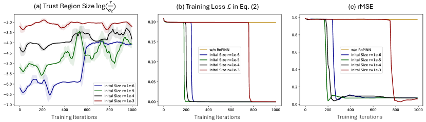
Figure 2: Optimization of canonical PINN [33] on the 1D-Reaction under different region sizes. To highlight the region size change, we adopt the moving average over time and mark the temporal standard deviation with shadow. The steep training loss is caused by the learning difficulty of PDE.

Number of sampling points in Eq. (8)

For efficiency, RoPINN only samples one point within the trust region to approximate the region gradient descent. However, it is worth noticing that sampling more points will make the approximation in Eq. (8) more accurate, which can further make the optimization process adapt to a larger region size $r$. Thus, as shown in Figure 2(a-b), sampling more points will also increase the finally learned region size $r$ and speed up the convergence. In addition, Figure 2(c) shows that adding sampled points can also improve the final performance, which has been proved in Theorem 3.5 that the upper bound of generalization error is proportion to region size.

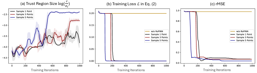
Figure 3: Optimization of canonical PINN [33] on the 1D-Reaction under different sample points.

Ablations

To verify the effectiveness of our design in RoPINN, we present ablations in Figure 4. It is observed that although we only sample one point, even fixed-size region optimization can also boost the performance of PINNs in most cases. However, as illustrated in Theorem 3.9, the sampling process may also cause estimation error, so the relative promotion is inconsistent and unstable among different PDEs and base models. With our proposed trust region calibration, we can obtain a more significant and consistent improvement, verifying the effectiveness of our design in RoPINN.

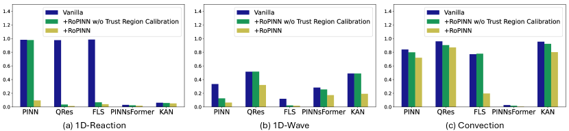
Figure 4: Ablation study of RoPINN on different PDEs and diverse base models. rMSE is recorded.

Loss landscape

Previous research [22] has studied why PINN cannot solve the Convection equation and found that it is not caused by the limited model capacity but by the hard-to-optimize loss landscape. Here we also provide a loss landscape visualization in Figure 5, which is obtained by perturbing the trained model along the directions of the first two dominant Hessian eigenvectors [22, 23, 49]. We can find that vanilla PINN optimized by PINN loss in Eq. (2) presents sharp cones. In contrast, empowered by RoPINN, the loss landscape is significantly smoothed. This visualization intuitively interprets why RoPINN can mitigate “PINN failure modes”. See Appendix D for more results.

Figure 5: Loss landscape of RoPINN and vanilla PINNs on Convection. Error refers to $(u_{\theta}-u)$.

5 Conclusion

This paper presents and analyzes a new PINN optimization paradigm: region optimization. Going beyond previous scatter-point optimization, we extend the optimization from selected points to their neighborhood regions. Based on this idea, RoPINN is implemented as a simple but effective training algorithm, where an effcient Monte Carlo approximation process is used along with a trust region calibration strategy to control the estimation error. In addition to theoretical advantages, RoPINN can consistently boost the performance of various advanced PINN models without extra backpropagation or gradient calculation, demonstrating favorable efficiency, training stability and general capability.

Appendix A Generalization Analysis in Section 3.1

This section will present the proofs for the theorems in Section 3.1.

A.1 Proof for Point Optimization Generalization Error (Theorem 3.3)

The proof for the convex case is derived from previous papers [13, 47] under the Assumption 3.2. We derive a more compact upper bound for generalization error in expectation for the non-convex setting.

Lemma A.1.

Given two finite sets of selected points $\mathcal{S}=(\boldsymbol{x}_{1},\cdots,\boldsymbol{x}_{N})$ and $\mathcal{S}^{\prime}=(\boldsymbol{x}_{1}^{\prime},\cdots,\boldsymbol{x}_{N}^{\prime})$, let $\mathcal{S}^{(i)}=(\boldsymbol{x}_{1},\cdots,\boldsymbol{x}_{i-1},\boldsymbol{x}_{i}^{\prime},\boldsymbol{x}_{i+1},\cdots,\boldsymbol{x}_{N})$ be the set that is identical to $\mathcal{S}$ except the $i$-th element, the generalization error in expectation is equal to the expectation of the error difference between these two sets, which can be formalized as follows:

$$\mathcal{E}_{\mathrm{gen}}=\left|\mathbb{E}_{\mathcal{S},\mathcal{S}^{\prime},\mathcal{A}}\left[\frac{1}{N}\sum_{i=1}^{N}\mathcal{L}(\mathcal{A}(\mathcal{S}^{(i)}),\boldsymbol{x}_{i}^{\prime})-\frac{1}{N}\sum_{i=1}^{N}\mathcal{L}(\mathcal{A}(\mathcal{S}),\boldsymbol{x}_{i}^{\prime})\right]\right|.$$ (15)

Proof.

Directly deriving from the in-domain loss, we have:

$$\begin{split}\mathbb{E}_{\mathcal{S},\mathcal{A}}\left[\mathcal{L}(\mathcal{A}(\mathcal{S}),\mathcal{S})\right]&=\mathbb{E}_{\mathcal{S},\mathcal{A}}\left[\frac{1}{N}\sum_{i=1}^{N}\mathcal{L}(\mathcal{A}(\mathcal{S}),\boldsymbol{x}_{i})\right]\\ &=\mathbb{E}_{\mathcal{S},\mathcal{S}^{\prime},\mathcal{A}}\left[\frac{1}{N}\sum_{i=1}^{N}\mathcal{L}(\mathcal{A}(\mathcal{S}^{(i)}),\boldsymbol{x}_{i}^{\prime})\right]\quad\quad\quad\quad\text{(Expectation on $\boldsymbol{x}_{i}^{\prime}$)}\\ &=\mathbb{E}_{\mathcal{S},\mathcal{S}^{\prime},\mathcal{A}}\left[\frac{1}{N}\sum_{i=1}^{N}\mathcal{L}(\mathcal{A}(\mathcal{S}),\boldsymbol{x}_{i}^{\prime})\right]+\delta\\ &=\mathbb{E}_{\mathcal{S},\mathcal{A}}\left[\mathcal{L}(\mathcal{A}(\mathcal{S}),\Omega)\right].\end{split}$$ (16)

Then, according to Definition 3.1, we have:

$$\begin{split}\mathcal{E}_{\mathrm{gen}}=\delta=\mathbb{E}_{\mathcal{S},\mathcal{S}^{\prime},\mathcal{A}}\left[\frac{1}{N}\sum_{i=1}^{N}\mathcal{L}(\mathcal{A}(\mathcal{S}^{(i)}),\boldsymbol{x}_{i}^{\prime})-\frac{1}{N}\sum_{i=1}^{N}\mathcal{L}(\mathcal{A}(\mathcal{S}),\boldsymbol{x}_{i}^{\prime})\right].\end{split}$$ (17)

∎

Lemma A.2 (Convex case).

Given the stochastic gradient method with an update rule as $G_{\alpha,\boldsymbol{x}}(\theta)=\theta-\alpha\nabla_{\theta}\mathcal{L}(\theta,\boldsymbol{x})$ and $\mathcal{L}$ is convex in $\theta$, then for $\alpha\leq\frac{2}{\beta}$, we have $\|G_{\alpha,\boldsymbol{x}}(\theta_{1})-G_{\alpha,\boldsymbol{x}}(\theta_{2})\|\leq\|\theta_{1}-\theta_{2}\|$.

Proof.

For clarity, we denote $g=\|\nabla_{\theta}\mathcal{L}(\theta_{1},\boldsymbol{x})-\nabla_{\theta}\mathcal{L}(\theta_{2},\boldsymbol{x})\|$. Then we have:

$$\begin{split}\|G_{\alpha,\boldsymbol{x}}(\theta_{1})-G_{\alpha,\boldsymbol{x}}(\theta_{2})\|^{2}&=\|\theta_{1}-\theta_{2}-\alpha(\nabla_{\theta}\mathcal{L}(\theta_{1},\boldsymbol{x})-\nabla_{\theta}\mathcal{L}(\theta_{2},\boldsymbol{x}))\|^{2}\\ &=\|\theta_{1}-\theta_{2}\|^{2}-2\alpha\left(\nabla_{\theta}\mathcal{L}(\theta_{1},\boldsymbol{x})-\nabla_{\theta}\mathcal{L}(\theta_{2},\boldsymbol{x})\right)^{\sf T}(\theta_{1}-\theta_{2})+\alpha^{2}g^{2}\\ &\leq\|\theta_{1}-\theta_{2}\|^{2}-\frac{2\alpha}{\beta}g^{2}+\alpha^{2}g^{2}\quad\quad\quad\quad\text{(Convexity and Assumption \ref{assump:lipschitz})}\\ &\leq\|\theta_{1}-\theta_{2}\|^{2}.\quad\quad\quad\quad\ \ \quad\quad\quad\quad\quad\quad\ \text{($\alpha\leq\frac{2}{\beta}$)}\end{split}$$ (18)

∎

Convex setting

Next, we will give the proof for the convex case of Theorem 3.3(1).

Proof.

According to Lemma A.1, we attempt to bound the generalization error in expectation $\mathcal{E}_{\mathrm{gen}}$ by analyzing the error difference between two selected sample sets. Denote that $\mathcal{S}$ and $\mathcal{S}^{\prime}$ are identical except for one point. Suppose that with the stochastic gradient method on these two sets, we can obtain two optimization trajectories $\{\theta_{t}\}_{t=1}^{T}$ and $\{\theta_{t}^{\prime}\}_{t=1}^{T}$ respectively. According to Assumption 3.2, we have the following inequality:

$$\mathbb{E}\left[|\mathcal{L}({u_{\theta_{t}}},\boldsymbol{x})-\mathcal{L}({u_{\theta_{t}^{\prime}}},\boldsymbol{x})|\right]\leq L\mathbb{E}\left[\|\theta_{t}-\theta_{t}^{\prime}\|\right].$$ (19)

Note that at the $t$-th step, with probability $(1-\frac{1}{|\mathcal{S}|})$, the example selected by the stochastic gradient method is the same in both $\mathcal{S}$ and $\mathcal{S}^{\prime}$. As for the other $\frac{1}{|\mathcal{S}|}$ probability, we have to deal with different selected samples. Thus, according to Lemma A.2, we have:

$$\begin{split}\mathbb{E}\left[\|\theta_{t+1}-\theta_{t+1}^{\prime}\|\right]&=(1-\frac{1}{|\mathcal{S}|})\mathbb{E}\left[G_{\alpha_{t},\boldsymbol{x}}(\theta_{t})-G_{\alpha_{t},\boldsymbol{x}}(\theta_{t}^{\prime})\right]+\frac{1}{|\mathcal{S}|}\mathbb{E}\left[G_{\alpha_{t},\boldsymbol{x}}(\theta_{t})-G_{\alpha_{t},\boldsymbol{x}^{\prime}}(\theta_{t}^{\prime})\right]\\ &\leq(1-\frac{1}{|\mathcal{S}|})\mathbb{E}[\|\theta_{t}-\theta_{t}^{\prime}\|]+\frac{1}{|\mathcal{S}|}\mathbb{E}\left[\|\theta_{t}-\theta_{t}^{\prime}\|+\|\alpha_{t}\nabla_{\theta}\mathcal{L}(u_{\theta},\boldsymbol{x})-\alpha_{t}\nabla_{\theta}\mathcal{L}(u_{\theta},\boldsymbol{x}^{\prime})\|\right].\\ \end{split}$$ (20)

Due to the $L$-Lipschitz assumption of $\mathcal{L}$, the gradient $\nabla_{\theta}\mathcal{L}(u_{\theta},\boldsymbol{x})$ is uniformly smaller than $L$, then:

$$\begin{split}\mathbb{E}\left[\|\theta_{t+1}-\theta_{t+1}^{\prime}\|\right]&\leq\mathbb{E}\left[\|\theta_{t}-\theta_{t}^{\prime}\|\right]+\frac{2\alpha_{t}L}{|\mathcal{S}|}.\end{split}$$ (21)

In summary, since both optimization trajectories start from the same initialization, namely $\theta_{0}=\theta_{0}^{\prime}$, the following inequality holds:

$$\begin{split}\mathbb{E}\left[|\mathcal{L}({u_{\theta_{T}}},\boldsymbol{x})-\mathcal{L}({u_{\theta_{T}^{\prime}}},\boldsymbol{x})|\right]\leq\frac{2L^{2}}{|\mathcal{S}|}\sum_{t=1}^{T}\alpha_{t}.\end{split}$$ (22)

From Lemma A.1, we have $\mathcal{E}_{\mathrm{gen}}\leq\frac{2L^{2}}{|\mathcal{S}|}\sum_{t=1}^{T}\alpha_{t}$. ∎

Lemma A.3 (Non-convex case).

Given the stochastic gradient method with an update rule as $G_{\alpha,\boldsymbol{x}}(\theta)=\theta-\alpha\nabla_{\theta}\mathcal{L}(\theta,\boldsymbol{x})$, then we have $\|G_{\alpha,\boldsymbol{x}}(\theta_{1})-G_{\alpha,\boldsymbol{x}}(\theta_{2})\|\leq(1+\alpha\beta)\|\theta_{1}-\theta_{2}\|$.

Proof.

This inequality can be easily obtained from the following:

$$\begin{split}\|G_{\alpha,\boldsymbol{x}}(\theta_{1})-G_{\alpha,\boldsymbol{x}}(\theta_{2})\|&=\|\theta_{1}-\theta_{2}-\alpha(\nabla_{\theta}\mathcal{L}(\theta_{1},\boldsymbol{x})-\nabla_{\theta}\mathcal{L}(\theta_{2},\boldsymbol{x}))\|\\ &=\|\theta_{1}-\theta_{2}\|+\alpha\|\nabla_{\theta}\mathcal{L}(\theta_{1},\boldsymbol{x})-\nabla_{\theta}\mathcal{L}(\theta_{2},\boldsymbol{x})\|\\ &\leq(1+\alpha\beta)\|\theta_{1}-\theta_{2}\|.\quad\quad\quad\quad\quad\quad\quad\quad\quad\quad\quad\quad\text{(Assumption \ref{assump:lipschitz})}\end{split}$$ (23)

∎

Non-convex setting

Finally, we will give the proof for the non-convex case in Theorem 3.3(2).

Proof.

We also consider the optimization trajectory $\{\theta_{t}\}_{t=1}^{T}$ and $\{\theta_{t}^{\prime}\}_{t=1}^{T}$ from $\mathcal{S}$ and $\mathcal{S}^{\prime}$, which are identical except for one element. Let $\delta_{t}=\|\theta_{t}-\theta_{t}^{\prime}\|$ and $t_{0}\in\{1,\cdots,|\mathcal{S}|\}$ be a considered iteration, then we have:

$$\begin{split}\mathbb{E}\left[|\mathcal{L}({u_{\theta_{T}}},\boldsymbol{x})-\mathcal{L}({u_{\theta_{T}^{\prime}}},\boldsymbol{x})|\right]&=\mathbb{P}(\delta_{t_{0}}=0)\mathbb{E}\left[|\mathcal{L}({u_{\theta_{T}}},\boldsymbol{x})-\mathcal{L}({u_{\theta_{T}^{\prime}}},\boldsymbol{x})||\delta_{t_{0}}=0\right]\\ &+\mathbb{P}(\delta_{t_{0}}\neq 0)\mathbb{E}\left[|\mathcal{L}({u_{\theta_{T}}},\boldsymbol{x})-\mathcal{L}({u_{\theta_{T}^{\prime}}},\boldsymbol{x})||\delta_{t_{0}}\neq 0\right]\\ &\leq L\mathbb{E}\left[\|\theta_{T}-\theta_{T}^{\prime}\||\delta_{t_{0}}=0\right]+\mathbb{P}(\delta_{t_{0}}\neq 0)C\quad\quad\text{(Upper bound of $\mathcal{L}$)}\\ &=\frac{Ct_{0}}{|\mathcal{S}|}+L\mathbb{E}\left[\|\theta_{T}-\theta_{T}^{\prime}\||\delta_{t_{0}}=0\right].\end{split}$$ (24)

Similar to the convex case, we analyze the expectation of parameter difference in the $(t+1)$-th iteration as follows. Since $\alpha\leq\frac{1}{\beta t}$, then we have:

$$\begin{split}\mathbb{E}\left[\|\theta_{t+1}-\theta_{t+1}^{\prime}\||\delta_{t_{0}}=0\right]&\leq(1-\frac{1}{|\mathcal{S}|})(1+\frac{1}{t})\mathbb{E}\left[\|\theta_{t}-\theta_{t}^{\prime}\|\right]+\frac{1}{|\mathcal{S}|}\mathbb{E}\left[\|\theta_{t}-\theta_{t}^{\prime}\|\right]+\frac{2L}{\beta t|\mathcal{S}|}\\ &\leq(1+\frac{1}{t}-\frac{1}{t|\mathcal{S}|})\mathbb{E}[\delta_{t}]+\frac{2L}{\beta t|\mathcal{S}|}\\ &\leq\mathrm{exp}(\frac{1}{t}-\frac{1}{t|\mathcal{S}|})\mathbb{E}[\delta_{t}]+\frac{2L}{\beta t|\mathcal{S}|}.\quad\quad\quad\quad\ \quad\quad\text{($1+x\leq\mathrm{exp}(x)$)}\end{split}$$ (25)

Accumulating the above in equations recursively, we have:

$$\begin{split}\mathbb{E}\left[\|\theta_{T}-\theta_{T}^{\prime}\||\delta_{t_{0}}=0\right]&\leq\sum_{t=t_{0}+1}^{T}\left\{\Pi_{k=t+1}^{T}\mathrm{exp}\left(\frac{1}{t}-\frac{1}{t|\mathcal{S}|}\right)\right\}\frac{2L}{\beta t|\mathcal{S}|}\\ &\leq\sum_{t=t_{0}+1}^{T}\mathrm{exp}\left((1-\frac{1}{|\mathcal{S}|})\log\frac{T}{t}\right)\frac{2L}{\beta t|\mathcal{S}|}\quad\quad\quad\quad\quad\quad\text{($\sum_{k=t+1}^{T}\frac{1}{k}\leq\log\frac{T}{t}$)}\\ &=\frac{2L}{\beta|\mathcal{S}|}T^{1-\frac{1}{|\mathcal{S}|}}\sum_{t=t_{0}+1}^{T}t^{-(1-\frac{1}{|\mathcal{S}|})-1}\\ &\leq\frac{2L}{\beta|\mathcal{S}|}T^{1-\frac{1}{|\mathcal{S}|}}\frac{1}{1-\frac{1}{|\mathcal{S}|}}\left(t_{0}^{-(1-\frac{1}{|\mathcal{S}|})}-T^{-(1-\frac{1}{|\mathcal{S}|})}\right).\quad\text{(Integral approximation)}\\ \end{split}$$ (26)

Organizing the above inequalities, we have:

$$\begin{split}\mathbb{E}\left[\|\theta_{T}-\theta_{T}^{\prime}\||\delta_{t_{0}}=0\right]&\leq\frac{2L}{\beta(|\mathcal{S}|-1)}\left(\frac{T}{t_{0}}\right)^{1-\frac{1}{|\mathcal{S}|}}-\frac{2L}{\beta(|\mathcal{S}|-1)}\\ &\leq\frac{2L}{\beta(|\mathcal{S}|-1)}\left(\frac{T}{t_{0}}\right)-\frac{2L}{\beta(|\mathcal{S}|-1)}.\end{split}$$ (27)

According to Eq. (24), for arbitrary $T\geq 1$, we just choose $t_{0}=1$, then

$$\begin{split}\mathbb{E}\left[|\mathcal{L}({u_{\theta_{T}}},\boldsymbol{x})-\mathcal{L}({u_{\theta_{T}^{\prime}}},\boldsymbol{x})|\right]&\leq\frac{C}{|\mathcal{S}|}+\frac{2L^{2}(T-1)}{\beta(|\mathcal{S}|-1)}.\end{split}$$ (28)

∎

This boundary is more tight than [13, 47], where the latter omits the $\frac{2L}{\beta(|\mathcal{S}|-1)}$ term in Eq. (27).

A.2 Proof for Properties of Region Optimization (Lemma 3.4)

Since $\mathcal{L}_{r}^{\mathrm{region}}$ is defined as a region integral of $\mathcal{L}$, Lemma 3.4 can be easily obtained by:

$$\begin{split}\text{Bounded:}\ \ \ \ &\mathcal{L}_{r}^{\mathrm{region}}(u_{\theta},\boldsymbol{x})=\frac{1}{|\Omega_{r}|}\int_{\Omega_{r}}\mathcal{L}(u_{\theta},\boldsymbol{x}+\boldsymbol{\xi})\mathrm{d}\boldsymbol{\xi}\leq\max_{\theta,\boldsymbol{x}}\mathcal{L}(u_{\theta},\boldsymbol{x})\\ \text{Convexity:}\ \ \ \ &\left(\nabla_{\theta}\mathcal{L}_{r}^{\mathrm{region}}(u_{\theta_{1}},\boldsymbol{x})-\nabla_{\theta}\mathcal{L}_{r}^{\mathrm{region}}(u_{\theta_{2}},\boldsymbol{x})\right)^{\sf T}(\theta_{1}-\theta_{2})\\ &=\frac{1}{|\Omega_{r}|}\int_{\Omega_{r}}\left(\nabla_{\theta}\mathcal{L}(u_{\theta_{1}},\boldsymbol{x}+\boldsymbol{\xi})-\nabla_{\theta}\mathcal{L}(u_{\theta_{2}},\boldsymbol{x}+\boldsymbol{\xi})\right)^{\sf T}(\theta_{1}-\theta_{2})\mathrm{d}\boldsymbol{\xi}\geq 0\\ \text{Lipschitz:}\ \ \ \ &\|\mathcal{L}_{r}^{\mathrm{region}}(u_{\theta_{1}},\boldsymbol{x})-\mathcal{L}_{r}^{\mathrm{region}}(u_{\theta_{2}},\boldsymbol{x})\|\\ &\leq\frac{1}{|\Omega_{r}|}\int_{\Omega_{r}}\left\|\mathcal{L}(u_{\theta_{1}},\boldsymbol{x}+\boldsymbol{\xi})-\mathcal{L}(u_{\theta_{2}},\boldsymbol{x}+\boldsymbol{\xi})\right\|\mathrm{d}\boldsymbol{\xi}\leq L\|\theta_{1}-\theta_{2}\|\\ \text{Smoothness:}\ \ \ \ &\|\nabla_{\theta}\mathcal{L}_{r}^{\mathrm{region}}(u_{\theta_{1}},\boldsymbol{x})-\nabla_{\theta}\mathcal{L}_{r}^{\mathrm{region}}(u_{\theta_{2}},\boldsymbol{x})\|\\ &\leq\frac{1}{|\Omega_{r}|}\int_{\Omega_{r}}\left\|\nabla_{\theta}\mathcal{L}(u_{\theta_{1}},\boldsymbol{x}+\boldsymbol{\xi})-\nabla_{\theta}\mathcal{L}(u_{\theta_{2}},\boldsymbol{x}+\boldsymbol{\xi})\right\|\mathrm{d}\boldsymbol{\xi}\leq\beta\|\theta_{1}-\theta_{2}\|.\end{split}$$ (29)

A.3 Proof for Region Optimization Generalization Error (Theorem 3.5)

Similar to the proof in Appendix A.1, we will discuss the generalization error on region optimization.

Convex setting

Firstly, we would like to prove the convex case as follows.

Proof.

According to Lemma 3.4, the region loss also holds the convexity, Lipschitz and smoothness properties, which ensures that Lemma A.2 and A.3 still work for $\mathcal{L}_{r}^{\mathrm{region}}$. We also focus on the selected sample sets $\mathcal{S}$ and $\mathcal{S}^{\prime}$, which are identical except for one element. Thus, at $t$-step, the following equation is satisfied:

$$\begin{split}\mathbb{E}\left[\|\theta_{t+1}-\theta_{t+1}^{\prime}\|\right]&=(1-\frac{1}{|\mathcal{S}|})\mathbb{E}\left[G^{\mathrm{region}}_{\alpha_{t},\boldsymbol{x}}(\theta_{t})-G^{\mathrm{region}}_{\alpha_{t},\boldsymbol{x}}(\theta_{t}^{\prime})\right]+\frac{1}{|\mathcal{S}|}\mathbb{E}\left[G^{\mathrm{region}}_{\alpha_{t},\boldsymbol{x}}(\theta_{t})-G^{\mathrm{region}}_{\alpha_{t},\boldsymbol{x}^{\prime}}(\theta_{t}^{\prime})\right]\\ &\leq(1-\frac{1}{|\mathcal{S}|})\mathbb{E}\left[\|\theta_{t}-\theta_{t}^{\prime}\|\right]+\frac{1}{|\mathcal{S}|}\mathbb{E}\left[G^{\mathrm{region}}_{\alpha_{t},\boldsymbol{x}}(\theta_{t})-G^{\mathrm{region}}_{\alpha_{t},\boldsymbol{x}^{\prime}}(\theta_{t}^{\prime})\right].\end{split}$$ (30)

As for the second item on the right part, we also consider the upper bound of $\nabla_{\theta}\mathcal{L}(u_{\theta},\boldsymbol{x})$. However, different from point-wise optimization, $\boldsymbol{x}+\Omega$ could overlap with $\boldsymbol{x}^{\prime}+\Omega$. Thus, we can obtain the following estimation for the difference between the updated model parameters:

$$\begin{split}&\mathbb{E}\left[G^{\mathrm{region}}_{\alpha_{t},\boldsymbol{x}}(\theta_{t})-G^{\mathrm{region}}_{\alpha_{t},\boldsymbol{x}^{\prime}}(\theta_{t}^{\prime})\right]\\ &\leq\frac{|\Omega|-|\Omega_{r}|}{|\Omega|}\mathbb{E}\left[\|\theta_{t}-\theta_{t}^{\prime}\|+2\alpha_{t}L\right]\quad\quad\quad\text{(Separate analysis for overlapped and non-overlap cases)}\\ &+\frac{|\Omega_{r}|}{|\Omega|}\mathbb{E}_{\Omega_{\mathrm{in}}}\left[\left\|\theta_{t}-\theta_{t}^{\prime}-\left(\alpha_{t}\frac{1}{|\Omega_{r}|}\int_{\Omega_{\mathrm{in}}}\nabla_{\theta}\mathcal{L}({u_{\theta_{t}}},\boldsymbol{x}+\boldsymbol{\xi})\mathrm{d}\boldsymbol{\xi}-\alpha_{t}\frac{1}{|\Omega_{r}|}\int_{\Omega_{\mathrm{in}}}\nabla_{\theta}\mathcal{L}({u_{\theta_{t}^{\prime}}},\boldsymbol{x}+\boldsymbol{\xi})\mathrm{d}\boldsymbol{\xi}\right)\right\|\right]\\ &+\frac{|\Omega_{r}|}{|\Omega|}\mathbb{E}_{\Omega_{\mathrm{in}}}\left[\frac{|\Omega_{r}|-|\Omega_{\mathrm{in}}|}{|\Omega_{r}|}2\alpha_{t}L\right]\\ &\leq\frac{|\Omega|-|\Omega_{r}|}{|\Omega|}\mathbb{E}\left[\|\theta_{t}-\theta_{t}^{\prime}\|+2\alpha_{t}L\right]+\frac{|\Omega_{r}|}{|\Omega|}\mathbb{E}_{\Omega_{\mathrm{in}}}\left[\|\theta_{t}-\theta_{t}^{\prime}\|+\frac{|\Omega_{r}|-|\Omega_{\mathrm{in}}|}{|\Omega_{r}|}2\alpha_{t}L\right]\\ &\leq\mathbb{E}\left[\|\theta_{t}-\theta_{t}^{\prime}\|\right]+2\alpha_{t}L(1-\frac{|\Omega_{r}|}{|\Omega|}+\frac{|\Omega_{r}|-\frac{|\Omega_{r}|^{2}}{2^{(d+1)}}}{|\Omega|})\\ &\leq\mathbb{E}\left[\|\theta_{t}-\theta_{t}^{\prime}\|\right]+2\alpha_{t}L(1-\frac{|\Omega_{r}|^{2}}{2^{(d+1)}|\Omega|}),\end{split}$$ (31)

where $\Omega_{\mathrm{in}}$ denotes the overlapped part between $\boldsymbol{x}+\Omega$ and $\boldsymbol{x}^{\prime}+\Omega$. In the above inequalities, the second inequality is based on the following derivation:

$$\begin{split}\left\|\alpha_{t}\frac{1}{|\Omega_{r}|}\int_{\Omega_{\mathrm{in}}}\nabla_{\theta}\mathcal{L}({u_{\theta_{t}}},\boldsymbol{x}+\boldsymbol{\xi})\mathrm{d}\boldsymbol{\xi}-\alpha_{t}\frac{1}{|\Omega_{r}|}\int_{\Omega_{\mathrm{in}}}\nabla_{\theta}\mathcal{L}({u_{\theta_{t}^{\prime}}},\boldsymbol{x}+\boldsymbol{\xi})\mathrm{d}\boldsymbol{\xi}\right\|&\leq\frac{|\Omega_{r}|}{|\Omega|}\frac{2}{\beta}\beta\|\theta_{t}-\theta_{t}^{\prime}\|\\ &\leq 2\|\theta_{t}-\theta_{t}^{\prime}\|.\end{split}$$ (32)

Thus, recursively accumulating the residual at the $t$-th step, we have:

$$\begin{split}\mathcal{E}_{\mathrm{gen}}\leq(1-\frac{|\Omega_{r}|^{2}}{2^{(d+1)}|\Omega|})\frac{2L^{2}}{|\mathcal{S}|}\sum_{t=1}^{T}\alpha_{t}.\end{split}$$ (33)

∎

Non-convex setting

Afterward, we will give a proof for the non-convex setting.

Proof.

For clarity, let $M=\frac{|\Omega_{r}|^{2}}{2^{(d+1)}|\Omega|}$. Then, we can rewrite the Eq. (25) as follows:

If $\mathbb{E}(\delta_{t})\leq\frac{2L}{\beta}$, we have:

$$\begin{split}\mathbb{E}\left[\|\theta_{t+1}-\theta_{t+1}^{\prime}\||\delta_{t_{0}}=0\right]&\leq(1-\frac{1}{|\mathcal{S}|})(1+\frac{1}{t})\mathbb{E}\left[\|\theta_{t}-\theta_{t}^{\prime}\|\right]\\ &+\frac{1}{|\mathcal{S}|}\left((1+\frac{M}{t})\mathbb{E}\left[\|\theta_{t}-\theta_{t}^{\prime}\|\right]+\frac{2L}{\beta t}(1-M)\right)\\ &\leq(1+\frac{1}{t}-\frac{1-M}{t|\mathcal{S}|})\mathbb{E}[\delta_{t}]+\frac{2L}{\beta t|\mathcal{S}|}(1-M)\\ &\leq\mathrm{exp}\left(\frac{1}{t}-\frac{1-M}{t|\mathcal{S}|}\right)\mathbb{E}[\delta_{t}]+\frac{2L}{\beta t|\mathcal{S}|}(1-M).\end{split}$$ (34)

Otherwise, we still take the following equation:

$$\begin{split}\mathbb{E}\left[\|\theta_{t+1}-\theta_{t+1}^{\prime}\||\delta_{t_{0}}=0\right]&\leq\mathrm{exp}\left(\frac{1}{t}-\frac{1}{t|\mathcal{S}|}\right)\mathbb{E}[\delta_{t}]+\frac{2L}{\beta t|\mathcal{S}|}\end{split}$$ (35)

Suppose that at the first $K$ steps $\mathbb{E}[\delta_{t_{0}+K}]\leq\frac{2L}{\beta}$, Accumulating the above in equations recursively, we have the error accumulated to the first $K$ steps as follows:

$$\begin{split}\Delta&=\sum_{t=t_{0}+1}^{t_{0}+K}\left\{\Pi_{k=t+1}^{t_{0}+K}\mathrm{exp}\left(\frac{1}{t}-\frac{1-M}{t|\mathcal{S}|}\right)\Pi_{k=t_{0}+K+1}^{T}\mathrm{exp}\left(\frac{1}{t}-\frac{1}{t|\mathcal{S}|}\right)\right\}\frac{2L}{\beta t|\mathcal{S}|}(1-M)\\ &\leq\sum_{t=t_{0}+1}^{t_{0}+K}\mathrm{exp}\left((1-\frac{1}{|\mathcal{S}|})\log\frac{T}{t_{0}+K}+(1-\frac{1-M}{|\mathcal{S}|})\log\frac{t_{0}+K}{t}\right)\frac{2L}{\beta t|\mathcal{S}|}(1-M)\\ &=\sum_{t=t_{0}+1}^{t_{0}+K}\mathrm{exp}\left((1-\frac{1}{|\mathcal{S}|})\log\frac{T}{t}+\frac{M}{|\mathcal{S}|}\log\frac{t_{0}+K}{t}\right)\frac{2L}{\beta t|\mathcal{S}|}(1-M)\\ &\leq\sum_{t=t_{0}+1}^{t_{0}+K}\mathrm{exp}\left((1-\frac{1}{|\mathcal{S}|})\log\frac{T}{t}\right)\frac{2L}{\beta t|\mathcal{S}|}(1-M)(\frac{t_{0}+K}{t})^{\frac{M}{|\mathcal{S}|}}\\ &\leq\sum_{t=t_{0}+1}^{t_{0}+K}\mathrm{exp}\left((1-\frac{1}{|\mathcal{S}|})\log\frac{T}{t}\right)\frac{2L}{\beta t|\mathcal{S}|}-\sum_{t=t_{0}+1}^{t_{0}+K}\mathrm{exp}\left((1-\frac{1}{|\mathcal{S}|})\log\frac{T}{t}\right)\frac{2L}{\beta t|\mathcal{S}|}(M^{2})\\ &=\sum_{t=t_{0}+1}^{t_{0}+K}\mathrm{exp}\left((1-\frac{1}{|\mathcal{S}|})\log\frac{T}{t}\right)\frac{2L}{\beta t|\mathcal{S}|}-JM^{2},\end{split}$$ (36)

where $J$ is a finite value that depends on the training property of beginning iterations, namely $K$ and $t_{0}$. The last inequality is from $(\frac{t_{0}+K}{t})^{\frac{M}{|\mathcal{S}|}}\leq(1+M)$, when $|\mathcal{S}|$ is sufficient enough.

Then, following a similar process as Theorem 3.3(2), we can obtain:

$$\mathbb{E}\left[\|\theta_{T}-\theta_{T}^{\prime}\||\delta_{t_{0}}=0\right]\leq\frac{2L}{\beta(|\mathcal{S}|-1)}(\frac{T}{t_{0}})-\frac{2L}{\beta(|\mathcal{S}|-1)}-JM^{2}.$$ (37)

With $t_{0}=1$, we have the generalization error under the non-convex case satisfies:

$$\mathbb{E}\left[|\mathcal{L}({u_{\theta_{T}}},\boldsymbol{x})-\mathcal{L}({u_{\theta_{T}^{\prime}}},\boldsymbol{x})|\right]\leq\frac{C}{|\mathcal{S}|}+\frac{2L^{2}(T-1)}{\beta(|\mathcal{S}|-1)}-JLM^{2}.$$ (38)

∎

A.4 Proof for High-order Constraint Optimization (Corollary 3.6)

First, we would like to prove the following Lemma.

Lemma A.4.

Suppose that $\mathcal{L}$ is bounded by $C$ for all $\theta,\boldsymbol{x}$ and is $L$-Lipschitz and $\beta$-smooth for $\theta$, then the first-order $j$-th dimension loss function $\frac{\partial}{\partial x_{j}}\mathcal{L}_{r}^{\mathrm{region}}$ is also bounded by $C$ for all $\theta,\boldsymbol{x}$ and is $2L$-Lipschitz and $2\beta$-smooth for $\theta$.

Proof.

For the bounded property, with the non-negative property of loss function, we have:

$$\begin{split}\frac{\partial}{\partial x_{j}}\mathcal{L}_{r}^{\mathrm{region}}(u_{\theta},\boldsymbol{x})&=\frac{\partial}{\partial x_{j}}\int_{\Omega_{r}}\mathcal{L}(u_{\theta},\boldsymbol{x}+\boldsymbol{\xi})\mathrm{d}\boldsymbol{\xi}=\int_{\Omega_{r}\backslash x_{j}}\mathcal{L}(u_{\theta},\boldsymbol{x}+\boldsymbol{\xi}_{r})-\mathcal{L}(u_{\theta},\boldsymbol{x}+\boldsymbol{\xi}_{0})\mathrm{d}\boldsymbol{\xi}\leq C,\end{split}$$ (39)

where $\boldsymbol{\xi}_{r}=(\cdots,r,\cdots)\in\Omega_{t}\backslash x_{j}$ and $\boldsymbol{\xi}_{0}=(\cdots,0,\cdots)\in\Omega_{t}\backslash x_{j}$.

As for the Lipschitz and smoothness, we can obtain the following inequalities:

$$\begin{split}\text{Lipschitz:}\ \ \ \ &\|\frac{\partial}{\partial x_{j}}\mathcal{L}_{r}^{\mathrm{region}}(u_{\theta_{1}},\boldsymbol{x})-\frac{\partial}{\partial x_{j}}\mathcal{L}_{r}^{\mathrm{region}}(u_{\theta_{2}},\boldsymbol{x})\|\\ &=\|\int_{\Omega_{r}\backslash x_{j}}\mathcal{L}(u_{\theta_{1}},\boldsymbol{x}+\boldsymbol{\xi}_{r})-\mathcal{L}(u_{\theta_{1}},\boldsymbol{x}+\boldsymbol{\xi}_{0})-\mathcal{L}(u_{\theta_{2}},\boldsymbol{x}+\boldsymbol{\xi}_{r})-\mathcal{L}(u_{\theta_{2}},\boldsymbol{x}+\boldsymbol{\xi}_{0})\mathrm{d}\boldsymbol{\xi}\|\\ &\leq\int_{\Omega_{r}\backslash x_{j}}\|\mathcal{L}(u_{\theta_{1}},\boldsymbol{x}+\boldsymbol{\xi}_{r})-\mathcal{L}(u_{\theta_{2}},\boldsymbol{x}+\boldsymbol{\xi}_{r})\|+\|\mathcal{L}(u_{\theta_{1}},\boldsymbol{x}+\boldsymbol{\xi}_{0})-\mathcal{L}(u_{\theta_{2}},\boldsymbol{x}+\boldsymbol{\xi}_{0})\|\mathrm{d}\boldsymbol{\xi}\\ &\leq 2L\|\theta_{1}-\theta_{2}\|\\ \text{Smoothness:}\ \ \ \ &\|\nabla_{\theta}\frac{\partial}{\partial x_{j}}\mathcal{L}_{r}^{\mathrm{region}}(u_{\theta_{1}},\boldsymbol{x})-\nabla_{\theta}\frac{\partial}{\partial x_{j}}\mathcal{L}_{r}^{\mathrm{region}}(u_{\theta_{2}},\boldsymbol{x})\|\\ &=\|\nabla_{\theta}\int_{\Omega_{r}\backslash x_{j}}\mathcal{L}(u_{\theta_{1}},\boldsymbol{x}+\boldsymbol{\xi}_{r})-\mathcal{L}(u_{\theta_{1}},\boldsymbol{x}+\boldsymbol{\xi}_{0})-\mathcal{L}(u_{\theta_{2}},\boldsymbol{x}+\boldsymbol{\xi}_{r})-\mathcal{L}(u_{\theta_{2}},\boldsymbol{x}+\boldsymbol{\xi}_{0})\mathrm{d}\boldsymbol{\xi}\|\\ &\leq\int_{\Omega_{r}\backslash x_{j}}\|\nabla_{\theta}\mathcal{L}(u_{\theta_{1}},\boldsymbol{x}+\boldsymbol{\xi}_{r})-\nabla_{\theta}\mathcal{L}(u_{\theta_{2}},\boldsymbol{x}+\boldsymbol{\xi}_{r})\|\mathrm{d}\boldsymbol{\xi}\\ &+\int_{\Omega_{r}\backslash x_{j}}\|\nabla_{\theta}\mathcal{L}(u_{\theta_{1}},\boldsymbol{x}+\boldsymbol{\xi}_{0})-\nabla_{\theta}\mathcal{L}(u_{\theta_{2}},\boldsymbol{x}+\boldsymbol{\xi}_{0})\|\mathrm{d}\boldsymbol{\xi}\\ &\leq 2\beta\|\theta_{1}-\theta_{2}\|.\\ \end{split}$$ (40)

Thus, $\frac{\partial}{\partial x_{j}}\mathcal{L}_{r}^{\mathrm{region}}$ is also bounded by $C$ for all $\theta,\boldsymbol{x}$ and is $2L$-Lipschitz and $2\beta$-smooth for $\theta$. ∎

Next, we will give the proof for Corollary 3.6.

Proof.

According to Lemma A.3, we have the gradient update operator $G_{\alpha,\boldsymbol{x}}^{\mathrm{region},x_{j}}$ for $\frac{\partial}{\partial x_{j}}\mathcal{L}_{r}^{\mathrm{region}}$ satisfies the following inequality:

$$G_{\alpha,\boldsymbol{x}}^{\mathrm{region},x_{j}}(\theta_{1})-G_{\alpha,\boldsymbol{x}}^{\mathrm{region},x_{j}}(\theta_{2})\leq(1+2\alpha\beta)\|\theta_{1}-\theta_{2}\|.$$ (41)

Let $M=\frac{|\Omega_{r}|^{2}}{2^{(d+1)}|\Omega|}$, since $\alpha\leq\frac{1}{2\beta t}$, we can rewrite the Eq. (34) as follows:

$$\begin{split}&\mathbb{E}\left[\|\theta_{t+1}-\theta_{t+1}^{\prime}\||\delta_{t_{0}}=0\right]\\ &\leq(1-\frac{1}{|\mathcal{S}|})(1+\frac{1}{t})\mathbb{E}\left[\|\theta_{t}-\theta_{t}^{\prime}\|\right]+\frac{1}{|\mathcal{S}|}\left((1+\frac{M}{t})\mathbb{E}\left[\|\theta_{t}-\theta_{t}^{\prime}\|\right]+\frac{2L}{\beta}(1-M)\right).\\ \end{split}$$ (42)

Thus, following the same derivation as Theorem 3.5, we have Corollary 3.6 holds. ∎

Appendix B Algorithm Analysis in Section 3.2

This section contains the proof for the theoretical analysis of our proposed algorithm in Section 3.2.

B.1 Proof for Convergence Rate of RoPINN (Theorem 3.8)

The crux of proof is to take expectation for Monte Carlo sampling.

Proof.

From Taylor expansion, there exist $\boldsymbol{x}^{\prime}$ such that:

$$\begin{split}\mathcal{L}_{r}^{\mathrm{region}}(u_{\theta_{t+1}},\boldsymbol{x})&=\mathcal{L}_{r}^{\mathrm{region}}(u_{\theta_{t}}-\alpha_{t}\nabla_{\theta}\mathcal{L}(u_{\theta_{t}},\boldsymbol{x}+\boldsymbol{\xi}),\boldsymbol{x})\\ &=\mathcal{L}_{r}^{\mathrm{region}}(u_{\theta_{t}},\boldsymbol{x})-\alpha_{t}\nabla_{\theta}\mathcal{L}(u_{\theta_{t}},\boldsymbol{x}+\boldsymbol{\xi})^{\sf T}\nabla_{\theta}\mathcal{L}_{r}^{\mathrm{region}}(u_{\theta_{t}},\boldsymbol{x})\\ &+\frac{1}{2}(\alpha_{t}\nabla_{\theta}\mathcal{L}(u_{\theta_{t}},\boldsymbol{x}))^{\sf T}\nabla_{\theta}^{2}\mathcal{L}_{r}^{\mathrm{region}}(u_{\theta_{t}},\boldsymbol{x}^{\prime})(\alpha_{t}\nabla_{\theta}\mathcal{L}(u_{\theta_{t}},\boldsymbol{x}))\\ &\leq\mathcal{L}_{r}^{\mathrm{region}}(u_{\theta_{t}},\boldsymbol{x})-\alpha_{t}\nabla_{\theta}\mathcal{L}(u_{\theta_{t}},\boldsymbol{x}+\boldsymbol{\xi})^{\sf T}\nabla_{\theta}\mathcal{L}_{r}^{\mathrm{region}}(u_{\theta_{t}},\boldsymbol{x})+\frac{\alpha_{t}^{2}L^{2}H}{2}.\end{split}$$ (43)

Taking expectations to $\boldsymbol{\xi}$ on both sides, since $\mathbb{E}[\nabla_{\theta}\mathcal{L}(u_{\theta_{t}},\boldsymbol{x}+\boldsymbol{\xi})]=\nabla_{\theta}\mathcal{L}_{r}^{\mathrm{region}}(u_{\theta_{t}},\boldsymbol{x}+\boldsymbol{\xi})$, we have:

$$\begin{split}\mathbb{E}\left[\mathcal{L}_{r}^{\mathrm{region}}(u_{\theta_{t+1}},\boldsymbol{x})\right]&\leq\mathbb{E}\left[\mathcal{L}_{r}^{\mathrm{region}}(u_{\theta_{t}},\boldsymbol{x})-\alpha_{t}\nabla_{\theta}\mathcal{L}(u_{\theta_{t}},\boldsymbol{x}+\boldsymbol{\xi})^{\sf T}\nabla_{\theta}\mathcal{L}_{r}^{\mathrm{region}}(u_{\theta_{t}},\boldsymbol{x})+\frac{\alpha_{t}^{2}L^{2}H}{2}\right]\\ &=\mathbb{E}\left[\mathcal{L}_{r}^{\mathrm{region}}(u_{\theta_{t}},\boldsymbol{x})\right]-\alpha_{t}\mathbb{E}\left[\left\|\nabla_{\theta}\mathcal{L}_{r}^{\mathrm{region}}(u_{\theta_{t}},\boldsymbol{x})\right\|^{2}\right]+\frac{\alpha_{t}^{2}L^{2}H}{2}.\end{split}$$ (44)

Rearranging the terms and accumulating over $T$ iterations, we have the following sum:

$$\begin{split}\sum_{t=0}^{T-1}\alpha_{t}\mathbb{E}\left[\left\|\nabla_{\theta}\mathcal{L}_{r}^{\mathrm{region}}(u_{\theta_{t}},\boldsymbol{x})\right\|^{2}\right]&\leq\sum_{t=0}^{T-1}\left(\mathbb{E}\left[\mathcal{L}_{r}^{\mathrm{region}}(u_{\theta_{t}},\boldsymbol{x})\right]-\mathbb{E}\left[\mathcal{L}_{r}^{\mathrm{region}}(u_{\theta_{t+1}},\boldsymbol{x})\right]\right)+\sum_{t=0}^{T-1}\frac{\alpha_{t}^{2}L^{2}H}{2}\\ &\leq\mathcal{L}_{r}^{\mathrm{region}}(u_{\theta_{0}},\boldsymbol{x})-\mathcal{L}_{r}^{\mathrm{region}}(u_{\theta_{T}},\boldsymbol{x})+\frac{L^{2}H}{2}\sum_{t=0}^{T-1}\alpha_{t}^{2}\\ &\leq\mathcal{L}_{r}^{\mathrm{region}}(u_{\theta_{0}},\boldsymbol{x})-\mathcal{L}_{r}^{\mathrm{region}}(u_{\ast},\boldsymbol{x})+\frac{L^{2}H}{2}\sum_{t=0}^{T-1}\alpha_{t}^{2},\end{split}$$ (45)

where $u_{\ast}$ represents the global optimum. Here we run the gradient descent for a random number of iterations $\tau$. For $\tau=t$ iterations with probability:

$$\begin{split}\mathbb{P}(\tau=t)=\frac{\alpha_{t}}{\sum_{k=0}^{T-1}\alpha_{k}},\end{split}$$ (46)

Thus, with $\alpha_{t}=\frac{1}{\sqrt{t+1}}$, we have the gradient norm is bounded by:

$$\begin{split}\mathbb{E}\left[\left\|\nabla_{\theta}\mathcal{L}_{r}^{\mathrm{region}}(u_{\theta_{\tau}},\boldsymbol{x})\right\|^{2}\right]&=\left(\sum_{t=0}^{T-1}\alpha_{t}\right)^{-1}\sum_{t=0}^{T-1}\alpha_{t}\mathbb{E}\left[\left\|\nabla_{\theta}\mathcal{L}_{r}^{\mathrm{region}}(u_{\theta_{t}},\boldsymbol{x})\right\|^{2}\right]\\ &\leq\left(\sum_{t=0}^{T-1}\alpha_{t}\right)^{-1}\left(\mathcal{L}_{r}^{\mathrm{region}}(u_{\theta_{0}},\boldsymbol{x})-\mathcal{L}_{r}^{\mathrm{region}}(u_{\ast},\boldsymbol{x})+\frac{L^{2}H}{2}\sum_{t=0}^{T-1}\alpha_{t}^{2}\right)\\ &\lesssim(2\sqrt{T})^{-1}\left(\mathcal{L}_{r}^{\mathrm{region}}(u_{\theta_{0}},\boldsymbol{x})-\mathcal{L}_{r}^{\mathrm{region}}(u_{\ast},\boldsymbol{x})+\frac{L^{2}H}{2}\log(T+1)\right)\\ &=\mathcal{O}(\frac{1}{\sqrt{T}}).\end{split}$$ (47)

∎

B.2 Proof for Estimation of RoPINN (Theorem 3.9)

As presented in Eq. (8) and (44), we approximate the region optimization with the Monte Carlo sampling method. For better efficiency, we propose to only sample one point at each iteration. However, this will cause an estimation error formalized in Theorem 3.9, which can be directly derived by the definition of standard deviation.

B.3 Proof for Estimation of Trust Region (Lemma 3.10 and Theorem 3.11)

First, we give the proof for Lemma 3.10.

Proof.

According to Assumption 3.2, there exist $\boldsymbol{x}^{\prime}$, such that the following equation holds:

$$\begin{split}&\|\nabla_{\theta}\mathcal{L}(u_{\theta_{t}},\boldsymbol{z}_{1})-\nabla_{\theta}\mathcal{L}(u_{\theta_{t-1}},\boldsymbol{z}_{2})\|\\ &=\|\nabla_{\theta}\mathcal{L}(u_{\theta_{t}},\boldsymbol{z}_{1})-\nabla_{\theta}\mathcal{L}(u_{\theta_{t}}+\alpha_{t-1}\nabla_{\theta}\mathcal{L}(u_{\theta_{t-1}},\boldsymbol{z}_{2}),\boldsymbol{z}_{2})\|\\ &=\|\nabla_{\theta}\mathcal{L}(u_{\theta_{t}},\boldsymbol{z}_{1})-\nabla_{\theta}\mathcal{L}(u_{\theta_{t}},\boldsymbol{z}_{2})+\alpha_{t-1}\nabla_{\theta}\mathcal{L}(u_{\theta_{t-1}},\boldsymbol{z}_{2})\nabla^{2}_{\theta}\mathcal{L}(u_{\theta_{t-1}},\boldsymbol{x}^{\prime})\|\\ &\leq\|\nabla_{\theta}\mathcal{L}(u_{\theta_{t}},\boldsymbol{z}_{1})-\nabla_{\theta}\mathcal{L}(u_{\theta_{t}},\boldsymbol{z}_{2})\|+\alpha_{t-1}L\beta.\end{split}$$ (48)

∎

Next, we will prove Theorem 3.11.

Proof.

This theorem can be proved by demonstrating that: for all $i,j\in\{1,\cdots,{T_{0}}\}$:

$$\begin{split}\lim_{t\to\infty}\nabla_{\theta}\mathcal{L}(u_{\theta_{t-i+1}},z_{i})&=\nabla_{\theta}\mathcal{L}(u_{\theta_{t}},z_{i})\\ \lim_{t\to\infty}\nabla_{\theta}\mathcal{L}(u_{\theta_{t-i+1}},z_{i})-\nabla_{\theta}\mathcal{L}(u_{\theta_{t-j+1}},z_{j})&=\nabla_{\theta}\mathcal{L}(u_{\theta_{t}},z_{i})-\nabla_{\theta}\mathcal{L}(u_{\theta_{t}},z_{j}).\end{split}$$ (49)

For the first equation, since $\alpha_{t}\to 0$, given $\forall\epsilon$, there exists a constant $M$ such that any $t>M$, $\alpha_{t}\leq\frac{\epsilon}{{T_{0}}L\beta}$. Thus, for any $t>M$ and any $i,j\in\{1,\cdots,{T_{0}}\}$, the following equation is satisfied:

$$\begin{split}\|\nabla_{\theta}\mathcal{L}(u_{\theta_{t-i+1}},z_{i})-\nabla_{\theta}\mathcal{L}(u_{\theta_{t}},z_{i})\|&\leq\sum_{k=1}^{i-1}\|\nabla_{\theta}\mathcal{L}(u_{\theta_{t-i+k}},z_{i})-\nabla_{\theta}\mathcal{L}(u_{\theta_{t-i+k+1}},z_{i})\|\\ &\leq\sum_{k=1}^{i-1}\alpha_{t-i+k}L\beta\leq\epsilon.\end{split}$$ (50)

Thus, $\lim_{t\to\infty}\nabla_{\theta}\mathcal{L}(u_{\theta_{t-i+1}},z_{i})=\nabla_{\theta}\mathcal{L}(u_{\theta_{t}},z_{i})$. Therefore, given $\forall\epsilon^{\prime}$, there exist a constant $M^{\prime}$, $\forall t>M^{\prime}$, $\|\nabla_{\theta}\mathcal{L}(u_{\theta_{t-i+1}},z_{i})-\nabla_{\theta}\mathcal{L}(u_{\theta_{t}},z_{i})\|\leq\frac{\epsilon}{2}$.

As for the second equation, for any $t>M^{\prime}$, the following equation is satisfied:

$$\begin{split}&\|\nabla_{\theta}\mathcal{L}(u_{\theta_{t-i+1}},z_{i})-\nabla_{\theta}\mathcal{L}(u_{\theta_{t-j+1}},z_{j})-\nabla_{\theta}\mathcal{L}(u_{\theta_{t}},z_{i})-\nabla_{\theta}\mathcal{L}(u_{\theta_{t}},z_{j})\|\\ &\leq\|\nabla_{\theta}\mathcal{L}(u_{\theta_{t-i+1}},z_{i})-\nabla_{\theta}\mathcal{L}(u_{\theta_{t}},z_{i})\|+\|\nabla_{\theta}\mathcal{L}(u_{\theta_{t-j+1}},z_{j})-\nabla_{\theta}\mathcal{L}(u_{\theta_{t}},z_{j})\|\leq\epsilon^{\prime}.\end{split}$$ (51)

Thus, Theorem 3.11 can be proved by replacing the gradient of past iterations with their limitations. ∎

Appendix C Implementation Details

This section provides experiment details, including benchmarks, metrics and implementations.

C.1 Benchmarks

To comprehensively test our algorithm, we include the following four benchmarks. The first three benchmarks cover three typical PDEs (plotted in Figure 6), which are widely used in exploring the PINN optimization [22, 34]. The last one is an advanced comprehensive benchmark with 20 different PDEs. Here are the details.

Figure 6: Visualization of the solution $u$ for the first three benchmarks.

1D-Reaction

This problem is a one-dimensional non-linear ODE, which describes the chemical reactions. The concrete equation that we studied here can be formalized as follows:

$$\begin{split}\frac{\partial u}{\partial t}-\rho u(1-u)=0,&\ x\in(0,2\pi),t\in(0,1),\\ u(x,0)=\exp{\left(-\frac{(x-\pi)^{2}}{2(\pi/4)^{2}}\right)},&\ x\in[0,2\pi],\\ u(0,t)=u(2\pi,t),&\ t\in[0,1].\end{split}$$ (52)

The analytical solution to this problem is $u(x,t)=\frac{h(x)e^{\rho t}}{h(x)e^{\rho t}+1-h(x)}$ and $h(x)=\exp{\left(-\frac{(x-\pi)}{2(\pi/4)^{2}}\right)}$. In our experiments, we set $\rho=5$. This problem is previously studied as “PINN failure mode” [22], which is because of the non-linear term of the equation [27]. Besides, as shown in Figure 6(a), it contains sharp boundaries for the center high-value area, which is also hard to learn for deep models.

Following experiments in PINNsFormer [53], we uniformly sampled 101 points for initial state $\Omega_{0}$ and boundary $\partial\Omega$ and a uniform grid of 101$\times$101 mesh points for the residual domain $\Omega$. For evaluation, we employed a 101$\times$101 mesh within the residual domain $\Omega$. This strategy is also adopted for 1D-Wave and Convection experiments.

1D-Wave

This problem presents a hyperbolic PDE that is widely studied in acoustics, electromagnetism, and fluid dynamics [1]. Concretely, the PDE can be formalized as follows:

$$\begin{split}\frac{\partial^{2}u}{\partial t^{2}}-4\frac{\partial^{2}u}{\partial x^{2}}=0,&\ x\in(0,1),t\in(0,1),\\ u(x,0)=\sin(\pi x)+\frac{1}{2}\sin(\beta\pi x),&\ x\in[0,1],\\ \frac{\partial u(x,0)}{\partial t}=0,&\ x\in[0,1],\\ u(0,t)=u(1,t)=0,&\ t\in[0,1].\end{split}$$ (53)

The analytic solution for this PDE is $u(x,t)=\sin(\pi x)\cos(2\pi t)+\frac{1}{2}\sin(\beta\pi x)\cos(2\beta\pi t)$. We set $\beta=3$ for our experiments. As presented in Figure 6(b), the solution is smoother than the other two datasets, thereby easier for deep models to solve in some aspects. However, the equation contains second-order derivative terms, which also brings challenges in automatic differentiation. That is why gPINN [50] fails in this task (Table 2).

Convection

This problem is also a hyperbolic PDE that can be used to model fluid, atmosphere, heat transfer and biological processes [38]. The concrete PDE that we studied in this paper is:

$$\begin{split}\frac{\partial u}{\partial t}+\beta\frac{\partial u}{\partial t}=0,&\ x\in(0,2\pi),t\in(0,1),\\ u(x,0)=\sin(x),&\ x\in[0,2\pi],\\ u(0,t)=u(2\pi,t),&\ t\in[0,1].\end{split}$$ (54)

The analytic solution for this PDE is $u(x,t)=\sin(x-\beta t)$, where $\beta$ is set as 50 in our experiments. Note that although the final solution seems to be quite simple, it is difficult for PINNs in practice due to the highly complex and high-frequency patterns. And the previous research [22] has shown that the loss landscape of the Convection equation contains many hard-to-optimize sharp cones.

PINNacle

This benchmark [12] is built upon the DeepXDE [28], consisting of a wide range of PDEs and baselines. In their paper, the authors included 20 different PDE-solving tasks, covering diverse phenomena in fluid dynamics, heat conduction, etc and including PDEs with high dimensions, complex geometrics, nonlinearity and multiscale interactions. To ensure a comprehensive evaluation, we also benchmark RoPINN with PINNacle.

During our experiments, we found that there are several subtasks that none of the previous methods can solve, such as the 2D Heat equation with long time (Heat 2d-LT), 2D Navier-Stokes equation with long time (NS 2d-LT), 2D Wave equation with long time (Wave 2d-MS) and Kuramoto-Sivashinsky equation (KS). In addition to the challenges of high dimensionality and complex geometry mentioned by PINNacle, we discover unique challenges in these tasks caused by long periods and high-order derivatives of governed PDEs, making them extremely challenging for current PINNs. To solve these problems, we might need more powerful PINN backbones. Since we mainly focus on the PINN training paradigm, we omit the abovementioned 4 tasks to avoid the meaningless comparison and experiment with the left 16 tasks. Our datasets are summarized in Table 4.

Table 4: Details of datasets in PINNacle [12] (16 different PDEs included in our experiments), including the dimension of inputs, highest order of PDEs, number of train/test points and concrete equations. Here we only present the simplified PDE formalizations for intuitive understanding. More detailed descriptions of PDE type and coefficient meanings can be found in their paper [12].

PDE		Dimension	Order	$N_{\text{train}}$	$N_{\text{test}}$	Key Equations
Burges	1d-C	1D+Time	2	16384	12288	$\frac{\partial\boldsymbol{u}}{\partial t}+\boldsymbol{u}\cdot\nabla\boldsymbol{u}-\nu\Delta\boldsymbol{u}=0$
	2d-C	2D+Time	2	98308	82690
Poisson	2d-C	2D	2	12288	10240	$-\Delta\boldsymbol{u}=0$
	2d-CG	2D	2	12288	10240	$-\Delta\boldsymbol{u}+k^{2}\boldsymbol{u}=f(x,y)$
	3d-CG	3D	2	49152	40960	$-\mu_{i}\Delta\boldsymbol{u}+k_{i}^{2}\boldsymbol{u}=f(x,y,z),i=1,2$
	2d-MS	2D	2	12288	10329	$-\nabla(a(x)\nabla\boldsymbol{u})=f(x,y)$
Heat	2d-VC	2D+Time	2	65536	49189	$\frac{\partial\boldsymbol{u}}{\partial t}-\nabla(a(x)\nabla\boldsymbol{u})=f(x,t)$
	2d-MS	2D+Time	2	65536	49189	$\frac{\partial\boldsymbol{u}}{\partial t}-\frac{1}{(500\pi)^{2}}\boldsymbol{u}_{xx}-\frac{1}{\pi^{2}}\boldsymbol{u}_{yy}=0$
	2d-CG	2D+Time	2	65536	49152	$\frac{\partial\boldsymbol{u}}{\partial t}-\Delta\boldsymbol{u}=0$
NS	2d-C	2D	2	14337	12378	$\ \ \boldsymbol{u}\cdot\nabla\boldsymbol{u}+\nabla p-\frac{1}{Re}\Delta\boldsymbol{u}=0,\nabla\cdot\boldsymbol{u}=0$
	2d-CG	2D	2	14055	12007
Wave	1d-C	1D+Time	2	12288	10329	$\boldsymbol{u}_{tt}-4\boldsymbol{u}_{xx}=0$
	2d-CG	2D+Time	2	49170	42194	$\left[\nabla^{2}-\frac{1}{c(x)}\frac{\partial^{2}}{\partial t^{2}}\right]u(x,t)=0$
Chaotic	GS	2D+Time	2	65536	61780	$\boldsymbol{u}_{t}=\varepsilon_{1}\Delta\boldsymbol{u}+b(1-\boldsymbol{u})-\boldsymbol{u}\boldsymbol{v}^{2},\boldsymbol{v}_{t}=\varepsilon_{2}\Delta\boldsymbol{v}-d\boldsymbol{v}+\boldsymbol{uv}^{2}$
High-	PNd	5D	2	49152	67241	$-\Delta\boldsymbol{u}=\frac{\pi^{2}}{4}\sum_{i=1}^{n}\sin\left(\frac{\pi}{2}x_{i}\right)$
dim	HNd	5D+Time	2	65537	49152	$\frac{\partial\boldsymbol{u}}{\partial t}=k\Delta\boldsymbol{u}+f(x,t)$

C.2 Metrics

In our experiments, we adopt the following three metrics. Training loss, rMAE and rMSE. And the training loss has been defined in Eq. (2). Here are the calculations for rMSE and rMAE:

$$\text{rMAE: }\sqrt{\frac{\sum_{\boldsymbol{x}\in\mathcal{S}}\left|u_{\theta}(\boldsymbol{x})-u_{\ast}(\boldsymbol{x})\right|}{\sum_{\boldsymbol{x}\in\mathcal{S}}\left|u_{\ast}(\boldsymbol{x})\right|}}\quad\text{rMSE: }\sqrt{\frac{\sum_{\boldsymbol{x}\in\mathcal{S}}\left(u_{\theta}(\boldsymbol{x})-u_{\ast}(\boldsymbol{x})\right)^{2}}{\sum_{\boldsymbol{x}\in\mathcal{S}}\left(u_{\ast}(\boldsymbol{x})\right)^{2}}},$$ (55)

where $u_{\ast}$ denotes the ground truth solution. Note that the model output and ground truth can be negative and positive, respectively. Thus, these two metrics could be larger than 1.

C.3 Implementations

For classical base models PINN [33], QRes [3] and FLS [45], we adopt the conventional configuration from previous papers [53]. As for the latest model PINNsFormer [53] and KAN [26], we use their official code. Next, we will detail the implementations of optimization algorithms.

RoPINN

As we described in the main text, we set the initial region size $r=10^{-4}$, past iteration number $T_{0}=5$ and only sample 1 point for each region at each iteration for all datasets. The corresponding analyses have been included in Figure 2 for $r$, Figure 3 for sampling points and Appendix D.1 for $T_{0}$ to demonstrate the algorithm property under different hyperparameter settings.

In addition, our formalization for region optimization in Eq. (8) only involves the equation, initial and boundary conditions, where we can still calculate their loss values after random sampling in the extended region. This definition perfectly matches the setting of 1D-Reaction, 1D-Wave and Convection. However, in PINNacle [12], some tasks also involve the data loss term, such as the inverse problem (Appendix D.2), which means we can only obtain the correct values for several observed or pre-calculated points. Since these points are pre-selected, we cannot obtain their new values after sampling. Thus, we do not apply region sampling to these points in our experiments. Actually, the data loss term only involves the forward process of deep models, which is a pure data-driven paradigm and is distinct from the other PDE-derived terms in PINNs. Therefore, the previous methods, gPINN and vPINN, also do not consider the data loss term in their algorithms.

gPINN

For the first three benchmarks, we add the first-order derivatives for spatial and temporal dimensions as the regularization term. We also search the weights of regularization terms in $\{1,0.1,0.01\}$ and report the best results. As for the PINNacle, we report the results of canonical PINN following their paper [12] and experiment with other base models by only replacing the model.

vPINN

We follow the code base in PINNacle, and implement it to the first three benchmarks. The test functions are set as Legendre polynomials and the test function number is set as $5$. The number of points used to compute the integral within domain $\Omega$ is set as 10, and the number of grids is set differently for each subtask, with values of {4, 8, 16, 32} for PINNacle and the same to other baselines for the first three benchmarks.

Other baselines

In Table 3 of the main text, we also experiment with the loss-reweighting method NTK [42] and data-resampling method RAR [46]. For NTK, we follow their official code and recalculate the neural tangent kernel to update loss weights every 10 iterations. And the kernel size is set as 300. As for RAR, we use the residual-based adaptive refinement with distribution algorithm.

Appendix D Additional Results

In this section, we provide more results as a supplement to the main text, including additional hyperparameter analysis, new experiments and more showcases.

D.1 Hyperparameter Sensitivity on $T_{0}$

As we stated in Algorithm 1, we adopt the gradient variance of past $T_{0}$ iterations to approximate the sampling error defined in Theorem 3.9. In our experiments, we just choose $T_{0}=5$ for all benchmarks, which can already achieve a good performance. To analyze the effect of this hyperparameter, we further add experiments with different choices in Figure 7.

Figure 7: Hyperparameter analyses for $T_{0}$ in RoPINN based on PINN [33] and PINNsFormer [53] on different benchmarks. We change $T_{0}$ in $\{1,5,10,15,20,25,30\}$ and record the rMSE.

As shown in Figure 7, we can find that under all the choices in $\{1,5,10,15,20,25,30\}$, RoPINN performs better than the vanilla PINN. Specifically, in both 1D-Reaction and 1D-Wave (Figure 7(a-b)), the model performs quite stable under different choices of $T_{0}$. As for Convection in Figure 7(c-d), the influence of $T_{0}$ is relatively significant in PINN. This may caused by the deficiency of PINN in solving Convection, where all the PINN-based experiments fail to generate an accurate solution for Convection (rMSE>0.5, Table 2). If we adopt a more powerful base model, such as PINNsFormer [53], this sensitivity will be alleviated. Also, it is worth noticing that, even though in Convection, RoPINN surpasses the vanilla PINN under all hyperparameter settings of $T_{0}$.

Besides, we can observe that the model performance slightly decreases when we set $T_{0}$ with a relatively large value. This may come from the difference between parameters $\theta_{t}$ and $\theta_{t+29}$, which will make the gradient variance approximation less reliable (Eq. (50) in the Theorem 3.11 proof).

D.2 Experiments with Data Loss (Inverse Problem)

Table 5: Experiments on the Possion inverse problem (PInv) of PINNacle.

Method	rMAE	rMSE
PINN [33]	7.3e-2	8.2e-2
+gPINN [50]	7.3e-2 (-0.2%)	8.0e-2 (2.1%)
+vPINN [17]	1.3e+0	1.8e+0
+RoPINN	6.7e-2 (8.8%)	7.3e-2 (11.4%)

As we stated in the implementations (Appendix C.3), RoPINN can also be applied to tasks with data loss. Here we also include an inverse problem in PINNacle to testify to the performance of RoPINN in this case, which requires the model to reconstruct the diffusion coefficients of the Poisson equation from observations on 2500 uniform grids with additional Gaussian noise.

As presented in Table 5, in this task, RoPINN can also boost the performance of PINN with over 10% in the rMSE metric and outperform the other baselines (gPINN and vPINN) that cannot bring improvements. Note that in this experiment, we failed to reproduce the performance of vPINN reported by PINNacle. Thus, we report the results of vPINN by directly running the official code in PINNacle.

D.3 More Showcases

As a supplement to the main text, we provide the showcases of RoPINN in Figure 8. From these showcases, we can observe that RoPINN can consistently boost the model performance and benefit the solving process of boundaries, discontinuous phases and periodic patterns.

Figure 8: Showcases of RoPINN on the first three datasets based on PINN and PINNsFormer.

D.4 Standard Deviations

Considering the limited resources, we repeat all the experiments on the first three typical benchmarks and our method on the PINNacle three times and other experiments one time. The official paper of PINNacle has provided the standard deviations for PINN, gPINN and vPINN on all benchmarks.

We summarize the standard deviations of PINN in Table 6. As for other base models, the standard deviations of FLS, QRes and KAN are within 0.005 on 1D-Wave and Convection, and within 0.001 for 1D-Reaction. PINNsFormer’s standard deviations are smaller than 0.001 for all three benchmarks.

Table 6: Standard deviations for canonical PINN on three typical benchmarks. The confidence for RoPINN achieving the best performance is over 99% in all three benchmarks.

rMSE$\pm$Standard Deviations	1D-Reaction	1D-Wave	Convection
PINN [33]	0.981$\pm$5e-4	0.335$\pm$1e-3	0.840$\pm$5e-4
+gPINN [50]	0.978$\pm$3e-4	0.399$\pm$3e-3	0.935$\pm$3e-3
+vPINN [17]	0.982$\pm$3e-3	0.173$\pm$1e-3	0.743$\pm$2e-3
+RoPINN (Ours)	0.095$\pm$8e-4	0.064$\pm$1e-3	0.720$\pm$2e-3

Appendix E Full Results on PINNacle

In Table 2 of the main text, due to the context limitation, we only present the proportion of improved tasks over the total tasks. Here we provide the complete results for 5 based models for PINNacle (16 different tasks) in Table 7 and Table 8, where we can have the following observations:

• RoPINN presents favorable generality in varied PDEs and base models. As we described in Table 4, this benchmark contains of extensive physics phenomena. It is impressive that our proposed RoPINN can boost the performance of such extensive base models on a wide scope of PDEs, highlighting the generalizability of our algorithm.

• RoPINN is numerically stable and efficient for computation. As a training paradigm, RoPINN does not require extra gradient calculation and also does not add sampled points, which makes the algorithm computation efficient. In contrast, other baselines may generate poor results or encounter NaN or OOM problems in some PDEs.

Table 7: Full results of gPINN [50], vPINN [17] and RoPINN under different base models on PINNacle [12] (16 different PDEs). A lower rMAE or rMSE with higher relative promotion indicates better performance. The promotion over vanilla is recorded in parentheses. For clarity, we highlight the value with blue if it surpasses the vanilla PINN, gray if it fails (over 10 times worse than the vanilla PINN), or is numerically unstable (NaN) or out-of-memory (OOM).

(Part I)	PDE		Vanilla		gPINN [50]		vPINN [17]		RoPINN (Ours)
			rMAE	rMSE	rMAE	rMSE	rMAE	rMSE	rMAE	rMSE
PINN [33]	Burges	1d-C	1.1e-2	3.3e-2	3.7e-1	5.1e-1	4.0e-2 (-272.2%)	3.5e-1 (-952.3%)	9.1e-3 (15.8%)	1.4e-2 (56.6%)
		2d-C	4.5e-1	5.2e-1	4.9e-1 (-8.7%)	5.4e-1 (-3.8%)	6.6e-1 (-46.4%)	6.4e-1 (-23.0%)	4.3e-1 (4.0%)	4.9e-1 (5.3%)
	Poisson	2d-C	7.5e-1	6.8e-1	7.7e-1 (-3.0%)	7.0e-1 (-4.0%)	4.6e-1 (38.6%)	4.9e-1 (27.4%)	4.1e-1 (44.9%)	6.6e-1 (2.5%)
		2d-CG	5.4e-1	6.6e-1	7.4e-1 (-37.1%)	7.9e-1 (-21.0%)	2.4e-1 (54.7%)	2.9e-1 (56.4%)	4.1e-1 (24.1%)	6.0e-1 (8.1%)
		3d-CG	4.2e-1	5.0e-1	4.3e-1 (-4.2%)	5.2e-1 (-3.5%)	8.0e-1 (-91.4%)	7.4e-1 (-46.7%)	4.7e-1 (-11.9%)	4.6e-1 (8.7%)
		2d-MS	7.8e-1	6.4e-1	6.7e-1 (13.2%)	6.2e-1 (2.3%)	9.6e-1 (-23.6%)	9.7e-1 (-52.1%)	7.7e-1 (0.4%)	6.4e-1 (0.3%)
	Heat	2d-VC	1.2e+0	9.8e-1	1.9e+1	1.6e+1	8.8e-1 (26.9%)	9.4e-1 (4.5%)	8.7e-1 (27.6%)	7.9e-1 (19.7%)
		2d-MS	4.7e-2	6.9e-2	1.0e+0	8.5e-1	9.3e-1	9.3e-1	4.4e-2 (6.4%)	3.4e-2 (51.1%)
		2d-CG	2.7e-2	2.3e-2	1.9e-1 (-588.8%)	2.1e-1 (-787.3%)	3.1e+0	9.3e-1	1.5e-2 (43.5%)	2.0e-2 (12.6%)
	NS	2d-C	6.1e-2	5.1e-2	6.4e-1 (-958.6%)	4.9e-1 (-877.5%)	2.0e-1 (-225.2%)	2.9e-1 (-478.1%)	4.1e-2 (32.2%)	4.2e-2 (16.1%)
		2d-CG	1.8e-1	1.1e-1	4.2e-1 (-134.5%)	2.9e-1 (-167.6%)	9.9e-1 (-454.6%)	9.9e-1 (-812.2%)	1.5e-1 (19.0%)	9.8e-2 (10.2%)
	Wave	1d-C	5.5e-1	5.5e-1	7.0e-1 (-27.0%)	7.2e-1 (-31.9%)	1.4e+0 (-155.3%)	8.4e-1 (-53.5%)	3.8e-1 (31.1%)	3.9e-1 (28.0%)
		2d-CG	2.3e+0	1.6e+0	9.9e-1 (56.6%)	1.0e+0 (37.4%)	1.1e+0 (52.8%)	8.0e-1 (50.5%)	7.1e-1 (68.8%)	7.9e-1 (51.3%)
	Chaotic	GS	2.1e-2	9.4e-2	3.4e-2 (-61.0%)	9.5e-2 (-1.0%)	8.9e-1	1.2e+0	2.1e-2 (2.1%)	9.3e-2 (0.4%)
	High-	PNd	1.2e-3	1.1e-3	2.6e-3 (-119.5%)	2.7e-3 (-137.7%)	NaN	NaN	6.7e-4 (42.9%)	6.4e-4 (43.6%)
	dim	HNd	1.2e-2	5.3e-3	3.6e-3 (71.0%)	4.6e-3 (13.6%)	NaN	NaN	5.6e-4 (95.5%)	7.3e-4 (86.2%)
Proportion of improved tasks					18.8%	18.8%	25.0%	25.0%	93.8%	100.0%
QRes [3]	Burges	1d-C	5.8e-3	2.0e-2	3.6e-1	5.1e-1	2.0e-2 (-241.0%)	8.1e-2 (-309.3%)	5.7e-3 (1.4%)	1.8e-2 (6.8%)
		2d-C	3.2e-1	4.8e-1	4.9e-1 (-53.1%)	5.4e-1 (-11.1%)	1.1e+0 (-256.9%)	1.3e+0 (-161.2%)	3.2e-1 (0.3%)	4.7e-1 (1.8%)
	Poisson	2d-C	2.9e-1	6.8e-1	7.6e-1 (-159.4%)	7.2e-1 (-5.9%)	3.2e-1 (-7.6%)	3.0e-1 (55.6%)	2.9e-1 (0.6%)	7.0e-1 (-3.7%)
		2d-CG	3.1e-1	7.4e-1	7.3e-1 (-136.9%)	7.8e-1 (-6.0%)	6.4e-1 (-108.9%)	7.3e-1 (0.4%)	2.9e-1 (4.0%)	7.2e-1 (2.5%)
		3d-CG	9.0e-2	5.8e-1	5.9e-1 (-558.8%)	6.4e-1 (-10.7%)	8.0e-1 (-790.4%)	7.4e-1 (-28.4%)	8.9e-2 (1.2%)	5.6e-1 (3.5%)
		2d-MS	1.7e+0	7.9e-1	5.5e-1 (67.2%)	5.0e-1 (36.5%)	9.7e-1 (41.8%)	9.8e-1 (-24.4%)	1.9e+0 (-13.1%)	9.1e-1 (-15.0%)
	Heat	2d-VC	2.0e-1	1.3e+0	7.2e+0	5.9e+0 (-363.0%)	3.3e-1 (-63.9%)	3.2e-1 (74.9%)	1.6e-1 (19.6%)	1.1e+0 (16.8%)
		2d-MS	1.7e-2	1.4e-1	4.4e-1	3.5e-1 (-158.6%)	4.0e-1	3.8e-1 (-174.6%)	8.7e-3 (48.5%)	7.2e-2 (47.2%)
		2d-CG	1.9e-2	2.4e-2	1.1e-1 (-476.7%)	1.3e-1 (-440.1%)	6.1e-1	7.0e-1	2.0e-2 (-5.2%)	2.1e-2 (9.9%)
	NS	2d-C	3.9e-3	4.5e-2	3.9e-1	3.0e-1 (-565.9%)	2.8e-1	2.4e-1 (-427.7%)	2.1e-3 (47.6%)	3.4e-2 (23.6%)
		2d-CG	1.2e-2	7.7e-2	2.5e-1	1.6e-1 (-110.9%)	1.0e+0	1.0e+0	1.2e-2 (0.8%)	7.6e-2 (1.5%)
	Wave	1d-C	2.2e-1	4.8e-1	7.0e-1 (-216.0%)	7.1e-1 (-47.7%)	4.0e-2 (81.8%)	4.7e-1 (2.5%)	2.1e-1 (3.6%)	4.4e-1 (8.6%)
		2d-CG	1.5e-1	9.2e-1	9.8e-1 (-572.5%)	1.0e+0 (-8.4%)	1.3e+0 (-773.5%)	1.2e+0 (-29.6%)	2.2e-1 (-53.6%)	1.3e+0 (-38.3%)
	Chaotic	GS	1.1e-2	9.3e-2	2.0e-2 (-74.5%)	9.4e-2 (-0.3%)	8.6e-1	9.7e-1 (-937.8%)	9.9e-3 (13.2%)	9.2e-2 (1.8%)
	High-	PNd	1.5e-2	5.3e-3	3.4e-2 (-132.2%)	3.3e-2 (-532.7%)	NaN	NaN	5.7e-3 (60.5%)	1.8e-3 (66.5%)
	dim	HNd	2.9e-2	1.1e-2	2.1e-3 (92.7%)	2.1e-3 (81.4%)	NaN	NaN	2.1e-2 (25.6%)	8.3e-3 (25.8%)
Proportion of improved tasks					12.5%	12.5%	12.5%	25.0%	81.3%	81.3%
FLS [45]	Burges	1d-C	9.0e-3	1.4e-2	3.3e-1	4.8e-1	6.5e-2 (-620.9%)	3.0e-1	9.0e-3 (0.2%)	1.3e-2 (8.6%)
		2d-C	4.4e-1	4.9e-1	4.9e-1 (-13.0%)	5.4e-1 (-10.1%)	1.3e+0 (-195.0%)	1.3e+0 (-171.4%)	4.3e-1 (0.4%)	4.9e-1 (0.2%)
	Poisson	2d-C	6.8e-1	6.7e-1	7.3e-1 (-6.6%)	6.7e-1 (-1.2%)	9.0e-1 (-30.9%)	9.4e-1 (-40.5%)	7.2e-1 (-5.4%)	6.3e-1 (5.2%)
		2d-CG	6.3e-1	7.0e-1	7.8e-1 (-22.7%)	8.1e-1 (-16.2%)	6.0e-1 (5.6%)	7.0e-1 (-0.6%)	5.9e-1 (6.8%)	6.9e-1 (1.2%)
		3d-CG	4.2e-1	5.0e-1	4.5e-1 (-7.8%)	4.6e-1 (9.5%)	8.1e-1 (-95.5%)	7.5e-1 (-48.8%)	4.1e-1 (1.3%)	5.1e-1 (-0.5%)
		2d-MS	8.9e-1	7.5e-1	5.1e-1 (43.5%)	4.7e-1 (36.4%)	9.0e-1 (-0.0%)	9.4e-1 (-25.7%)	8.1e-1 (9.5%)	6.7e-1 (10.0%)
	Heat	2d-VC	1.5e+0	1.3e+0	3.4e+1	2.7e+1	1.2e+0 (16.9%)	1.1e+0 (11.5%)	1.2e+0 (21.1%)	1.1e+0 (17.2%)
		2d-MS	6.2e-2	4.8e-2	1.2e+0	9.0e-1	1.0e+0	9.9e-1	1.4e-1 (-132.3%)	8.4e-2 (-74.2%)
		2d-CG	1.5e-2	2.5e-2	9.9e-2 (-553.1%)	1.2e-1 (-394.9%)	3.4e+0	4.4e+0	1.2e-2 (20.4%)	2.5e-2 (0.6%)
	NS	2d-C	8.3e-2	6.9e-2	4.9e-1 (-483.0%)	3.7e-1 (-430.2%)	2.8e-1 (-236.9%)	2.5e-1 (-262.9%)	4.8e-2 (42.4%)	4.9e-2 (29.3%)
		2d-CG	1.8e-1	1.2e-1	3.9e-1 (-119.7%)	2.7e-1 (-124.6%)	9.9e-1 (-458.2%)	1.0e+0 (-727.3%)	1.4e-1 (19.8%)	9.9e-2 (18.0%)
	Wave	1d-C	4.0e-1	4.1e-1	6.3e-1 (-57.7%)	6.4e-1 (-55.7%)	1.1e-2 (97.2%)	1.1e-2 (97.3%)	3.8e-1 (5.3%)	3.9e-1 (4.9%)
		2d-CG	2.5e+0	2.4e+0	1.1e+0 (58.7%)	1.9e+0 (22.4%)	2.1e+0 (19.1%)	2.0e+0 (15.8%)	1.7e+0 (31.6%)	1.7e+0 (30.4%)
	Chaotic	GS	2.1e-2	9.4e-2	2.6e-1	2.4e-1 (-155.5%)	9.7e-1	1.0e+0	2.2e-2 (-5.8%)	9.0e-2 (3.9%)
	High-	PNd	8.9e-4	1.0e-3	2.0e-3 (-123.0%)	2.3e-3 (-127.2%)	NaN	NaN	5.4e-4 (39.6%)	6.4e-4 (37.5%)
	dim	HNd	3.7e-3	4.0e-3	9.6e-3 (-160.8%)	9.9e-3 (-144.2%)	NaN	NaN	1.3e-3 (63.8%)	1.4e-3 (66.1%)
Proportion of improved tasks					12.5%	18.8%	25.0%	18.8%	81.3%	87.5%

Table 8: Full results of gPINN [50], vPINN [17] and RoPINN under different base models on PINNacle [12] (16 different PDEs). A lower rMAE or rMSE with higher relative promotion indicates better performance. The promotion over vanilla is recorded in parentheses. For clarity, we highlight the value with blue if it surpasses the vanilla PINN, gray if it fails (over 10 times worse than the vanilla PINN), or is numerically unstable (NaN) or out-of-memory (OOM). For PINNsFormer, it fails in most of the tasks due to the OOM problem. We omit these tasks in calculating proportion.

(Part II)	PDE		Vanilla		gPINN [50]		vPINN [17]		RoPINN (Ours)
			rMAE	rMSE	rMAE	rMSE	rMAE	rMSE	rMAE	rMSE
PINNsformer [53]	Burges	1d-C	9.3e-3	1.4e-2	6.5e-1	6.7e-1	5.5e-1	5.7e-1	8.0e-3 (13.3%)	1.0e-2 (26.5%)
		2d-C	OOM	OOM	OOM (-%)	OOM (-%)	OOM (-%)	OOM (-%)	OOM (-%)	OOM (-%)
	Poisson	2d-C	7.2e-1	6.6e-1	1.0e+0 (-39.4%)	1.0e+0 (-52.7%)	1.0e+0 (-39.4%)	1.0e+0 (-52.7%)	6.9e-1 (4.1%)	6.2e-1 (5.9%)
		2d-CG	5.4e-1	6.3e-1	1.0e+0 (-86.6%)	1.0e+0 (-59.4%)	1.0e+0 (-86.6%)	1.0e+0 (-59.4%)	4.7e-1 (13.0%)	5.5e-1 (12.1%)
		3d-CG	OOM	OOM	OOM (-%)	OOM (-%)	OOM (-%)	OOM (-%)	OOM (-%)	OOM (-%)
		2d-MS	1.3e+0	1.1e+0	OOM	OOM	OOM	OOM	7.2e-1 (42.4%)	6.0e-1 (45.0%)
	Heat	2d-VC	OOM	OOM	OOM (-%)	OOM (-%)	OOM (-%)	OOM (-%)	OOM (-%)	OOM (-%)
		2d-MS	OOM	OOM	OOM (-%)	OOM (-%)	OOM (-%)	OOM (-%)	OOM (-%)	OOM (-%)
		2d-CG	OOM	OOM	OOM (-%)	OOM (-%)	OOM (-%)	OOM (-%)	OOM (-%)	OOM (-%)
	NS	2d-C	OOM	OOM	OOM (-%)	OOM (-%)	OOM (-%)	OOM (-%)	OOM (-%)	OOM (-%)
		2d-CG	1.0e-1	7.0e-2	7.4e-1 (-626.0%)	7.2e-1 (-939.9%)	1.0e+0 (-870.9%)	1.0e+0	9.8e-2 (4.7%)	6.3e-2 (9.0%)
	Wave	1d-C	5.0e-1	5.1e-1	8.3e-1 (-63.5%)	8.5e-1 (-65.5%)	5.2e-1 (-3.5%)	5.3e-1 (-3.4%)	4.7e-1 (7.4%)	4.8e-1 (6.8%)
		2d-CG	OOM	OOM	OOM (-%)	OOM (-%)	OOM (-%)	OOM (-%)	OOM (-%)	OOM (-%)
	Chaotic	GS	OOM	OOM	OOM (-%)	OOM (-%)	OOM (-%)	OOM (-%)	OOM (-%)	OOM (-%)
	High	PNd	OOM	OOM	OOM (-%)	OOM (-%)	OOM (-%)	OOM (-%)	OOM (-%)	OOM (-%)
	dim	HNd	OOM	OOM	OOM (-%)	OOM (-%)	OOM (-%)	OOM (-%)	OOM (-%)	OOM (-%)
Proportion of improved tasks					0.0%	0.0%	0.0%	0.0%	100.0%	100.0%
KAN [26]	Burges	1d-C	2.7e-1	5.4e-1	5.6e-1 (-111.8%)	6.7e-1 (-24.0%)	3.9e-1 (-47.5%)	5.5e-1 (-1.3%)	2.4e-1 (8.2%)	4.8e-1 (12.5%)
		2d-C	8.7e-1	9.4e-1	1.5e+0 (-71.8%)	1.7e+0 (-83.5%)	NaN	NaN	8.3e-1 (4.6%)	9.2e-1 (2.4%)
	Poisson	2d-C	7.3e-1	6.8e-1	7.4e-1 (-1.4%)	6.8e-1 (-0.1%)	1.6e-1 (78.2%)	1.5e-1 (78.4%)	6.3e-1 (13.4%)	6.8e-1 (-0.1%)
		2d-CG	7.7e-1	8.1e-1	8.1e-1 (-5.5%)	8.6e-1 (-6.9%)	6.5e-1 (14.9%)	7.3e-1 (9.8%)	6.5e-1 (15.8%)	6.9e-1 (14.0%)
		3d-CG	7.5e-1	1.4e+0	2.0e+0 (-163.6%)	1.8e+0 (-25.5%)	NaN	NaN	7.2e-1 (4.1%)	6.8e-1 (51.8%)
		2d-MS	9.5e-1	9.8e-1	1.0e+0 (-5.0%)	1.0e+0 (-2.7%)	9.9e-1 (-4.6%)	1.0e+0 (-2.3%)	9.2e-1 (3.4%)	9.6e-1 (2.1%)
	Heat	2d-VC	1.9e+1	1.5e+1	3.3e+0 (82.5%)	2.7e+0 (81.8%)	8.9e-1 (95.3%)	9.1e-1 (94.0%)	6.0e+0 (68.7%)	4.7e+0 (68.4%)
		2d-MS	1.4e+0	1.1e+0	2.0e+0 (-39.8%)	1.4e+0 (-28.4%)	8.3e-1 (42.8%)	7.5e-1 (31.4%)	7.4e-1 (49.1%)	6.9e-1 (36.8%)
		2d-CG	5.0e-1	5.3e-1	8.2e-1 (-63.1%)	7.3e-1 (-37.2%)	8.1e-1 (-60.8%)	9.0e-1 (-69.7%)	4.9e-1 (1.7%)	5.0e-1 (4.9%)
	NS	2d-C	5.0e-1	4.1e-1	8.1e-1 (-60.6%)	6.7e-1 (-65.8%)	2.1e-1 (57.7%)	1.7e-1 (58.6%)	4.1e-1 (18.2%)	3.9e-1 (2.9%)
		2d-CG	9.9e-1	6.4e-1	5.4e-1 (45.6%)	4.1e-1 (36.7%)	1.0e+0 (-1.1%)	1.0e+0 (-56.1%)	4.6e-1 (53.7%)	3.5e-1 (44.8%)
	Wave	1d-C	4.7e-1	4.7e-1	8.6e-1 (-85.2%)	8.8e-1 (-89.2%)	1.9e-1 (58.4%)	2.1e-1 (55.8%)	4.6e-1 (1.7%)	4.6e-1 (1.9%)
		2d-CG	1.7e+0	1.6e+0	1.1e+0 (37.4%)	1.1e+0 (33.4%)	NaN	NaN	9.8e-1 (43.2%)	9.6e-1 (41.1%)
	Chaotic	GS	NaN	NaN	1.1e+0 (-%)	9.4e-1 (-%)	8.5e-1 (-%)	9.6e-1 (-%)	7.5e-1 (-%)	7.0e-1 (-%)
	High-	PNd	4.6e-4	5.6e-4	2.8e-3 (-515.3%)	3.5e-3 (-518.4%)	NaN	NaN	3.7e-4 (19.9%)	5.3e-4 (5.5%)
	dim	HNd	1.9e-3	5.4e-3	5.9e-4 (68.9%)	8.0e-4 (85.3%)	NaN	NaN	1.5e-3 (20.8%)	6.5e-4 (88.0%)
Proportion of improved tasks					31.3%	31.3%	43.8%	43.8%	100.0%	93.8%

Appendix F Related Work

This section will discuss some related works as a supplement to Section 2. We will first discuss some PINN research and then we will also clarify some looking similar but completely distinct topics.

PINN optimizers

As we mentioned in the second paragraph of the introduction, many previous works focus on developing efficient and effective deep-model optimizers for PINNs [50, 34], which may help the optimization process tackle the ill-conditioned Hessian matrix or naturally balance multiple loss terms [48]. As we formalized in Algorithm 1, RoPINN is not restricted to a certain optimizer. The researchers can easily replace the Adam [20] or L-BFGS [25] with other advanced optimizers. Since we mainly focus on the objective function, these works are orthogonal to us.

Numerical differentiation for objective functions

In addition to the regularization or variational-based methods, some researchers attempt to replace the automatic differentiation with numerical approximations [36, 9], which can tackle the expensive computation cost caused by calculating high-order derivatives. However, this paradigm does not attempt to change the objection function definition, just focuses on the calculation of point optimization PINN loss, which is distinct from our proposed region optimization paradigm.

In addition, RoPINN is also distinct from data augmentation or adversarial training techniques in the following aspects: (1) Theorem difference: although our proposed practical algorithm is based on Monte Carlo sampling in a region, the underlying theoretical support and insights are a region-based objective function (Theorem 3.5). (2) Implementation difference: In our algorithm, not only is the input changed, but the objective is also correspondingly changed. Thus, this paper is foundationally different from augmentation and adversarial training in that the ground truth label is fixed. Our design is tailored to the physics-informed loss function of PINNs, where we can accurately calculate the equation residual at any point within the input domain.

Appendix G Limitations

This paper presents region optimization as a new PINN training paradigm and provides both theoretical analysis and practical algorithms, supported by extensive experiments. However, there are still several limitations. In the theoretical analysis, we assume that the canonical loss function is $L$-Lipschitz-$\beta$-smooth, which may not be guaranteed in practice. Besides, RoPINN involves several hyperparameters, such as initial region size $r$, and number of past iterations $T_{0}$. Although we have studied the sensitivity w.r.t. them in Figures 2 and Appendix D.1 and demonstrate that they are easy to tune in most cases, we still need to adjust them for better performance in practice. Some hyperparameter tuning tools, such as Weights and Bias (Wandb), may mitigate this limitation to some extent, which has already been used in previous related work [34].

References

- [1] Michael Francis Atiyah, Raoul Bott, and Lars Gårding. Lacunas for hyperbolic differential operators with constant coefficients i. 1970.
- [2] James Bradbury, Roy Frostig, Peter Hawkins, Matthew James Johnson, Chris Leary, Dougal Maclaurin, George Necula, Adam Paszke, Jake VanderPlas, Skye Wanderman-Milne, and Qiao Zhang. JAX: composable transformations of Python+NumPy programs, 2018.
- [3] Jie Bu and Anuj Karpatne. Quadratic residual networks: A new class of neural networks for solving forward and inverse problems in physics involving pdes. In SIAM, 2021.
- [4] Jacob Devlin, Ming-Wei Chang, Kenton Lee, and Kristina Toutanova. Bert: Pre-training of deep bidirectional transformers for language understanding. In NAACL, 2019.
- [5] Gouri Dhatt, Emmanuel Lefrançois, and Gilbert Touzot. Finite element method. John Wiley & Sons, 2012.
- [6] Lawrence C Evans. Partial differential equations. American Mathematical Soc., 2010.
- [7] Bengt Fornberg. A practical guide to pseudospectral methods. Cambridge university press, 1998.
- [8] Olga Fuks and Hamdi A Tchelepi. Limitations of physics informed machine learning for nonlinear two-phase transport in porous media. Journal of Machine Learning for Modeling and Computing, 2020.
- [9] Han Gao, Luning Sun, and Jian-Xun Wang. Phygeonet: Physics-informed geometry-adaptive convolutional neural networks for solving parameterized steady-state pdes on irregular domain. Journal of Computational Physics, 2021.
- [10] Christian Grossmann, Hans-Görg Roos, and Martin Stynes. Numerical treatment of partial differential equations. Springer, 2007.
- [11] Zhongkai Hao, Songming Liu, Yichi Zhang, Chengyang Ying, Yao Feng, Hang Su, and Jun Zhu. Physics-informed machine learning: A survey on problems, methods and applications. arXiv preprint arXiv:2211.08064, 2022.
- [12] Zhongkai Hao, Jiachen Yao, Chang Su, Hang Su, Ziao Wang, Fanzhi Lu, Zeyu Xia, Yichi Zhang, Songming Liu, Lu Lu, et al. Pinnacle: A comprehensive benchmark of physics-informed neural networks for solving pdes. arXiv preprint arXiv:2306.08827, 2023.
- [13] Moritz Hardt, Ben Recht, and Yoram Singer. Train faster, generalize better: Stability of stochastic gradient descent. In ICML, 2016.
- [14] Kaiming He, X. Zhang, Shaoqing Ren, and Jian Sun. Deep residual learning for image recognition. CVPR, 2016.
- [15] Arthur Jacot, Franck Gabriel, and Clément Hongler. Neural tangent kernel: Convergence and generalization in neural networks. NeurIPS, 2018.
- [16] George Em Karniadakis, Ioannis G Kevrekidis, Lu Lu, Paris Perdikaris, Sifan Wang, and Liu Yang. Physics-informed machine learning. Nat. Rev. Phys., 2021.
- [17] Ehsan Kharazmi, Zhongqiang Zhang, and George Em Karniadakis. Variational physics-informed neural networks for solving partial differential equations. arXiv preprint arXiv:1912.00873, 2019.
- [18] Ehsan Kharazmi, Zhongqiang Zhang, and George Em Karniadakis. hp-vpinns: Variational physics-informed neural networks with domain decomposition. Computer Methods in Applied Mechanics and Engineering, 2021.
- [19] Reza Khodayi-Mehr and Michael Zavlanos. Varnet: Variational neural networks for the solution of partial differential equations. In Learning for Dynamics and Control, 2020.
- [20] Diederik P. Kingma and Jimmy Ba. Adam: A method for stochastic optimization. In ICLR, 2015.
- [21] David A Kopriva. Implementing spectral methods for partial differential equations: Algorithms for scientists and engineers. Springer Science & Business Media, 2009.
- [22] Aditi Krishnapriyan, Amir Gholami, Shandian Zhe, Robert Kirby, and Michael W Mahoney. Characterizing possible failure modes in physics-informed neural networks. NeurIPS, 2021.
- [23] Hao Li, Zheng Xu, Gavin Taylor, Christoph Studer, and Tom Goldstein. Visualizing the loss landscape of neural nets. NeurIPS, 2018.
- [24] Zongyi Li, Nikola Borislavov Kovachki, Kamyar Azizzadenesheli, Burigede liu, Kaushik Bhattacharya, Andrew Stuart, and Anima Anandkumar. Fourier neural operator for parametric partial differential equations. In ICLR, 2021.
- [25] Dong C Liu and Jorge Nocedal. On the limited memory bfgs method for large scale optimization. Mathematical programming, 1989.
- [26] Ziming Liu, Yixuan Wang, Sachin Vaidya, Fabian Ruehle, James Halverson, Marin Soljačić, Thomas Y Hou, and Max Tegmark. Kan: Kolmogorov-arnold networks. arXiv preprint arXiv:2404.19756, 2024.
- [27] ES Lobanova and FI Ataullakhanov. Running pulses of complex shape in a reaction-diffusion model. Physical review letters, 2004.
- [28] Lu Lu, Xuhui Meng, Zhiping Mao, and George Em Karniadakis. DeepXDE: A deep learning library for solving differential equations. SIAM Review, 2021.
- [29] Suryanarayana Maddu, Dominik Sturm, Christian L Müller, and Ivo F Sbalzarini. Inverse dirichlet weighting enables reliable training of physics informed neural networks. Machine Learning: Science and Technology, 2022.
- [30] Rambod Mojgani, Maciej Balajewicz, and Pedram Hassanzadeh. Lagrangian pinns: A causality-conforming solution to failure modes of physics-informed neural networks. arXiv preprint arXiv:2205.02902, 2022.
- [31] Adam Paszke, S. Gross, Francisco Massa, A. Lerer, James Bradbury, Gregory Chanan, Trevor Killeen, Z. Lin, N. Gimelshein, L. Antiga, Alban Desmaison, Andreas Köpf, Edward Yang, Zach DeVito, Martin Raison, Alykhan Tejani, Sasank Chilamkurthy, Benoit Steiner, Lu Fang, Junjie Bai, and Soumith Chintala. Pytorch: An imperative style, high-performance deep learning library. In NeurIPS, 2019.
- [32] Maziar Raissi. Deep hidden physics models: Deep learning of nonlinear partial differential equations. JMLR, 2018.
- [33] Maziar Raissi, Paris Perdikaris, and George Em Karniadakis. Physics-informed neural networks: A deep learning framework for solving forward and inverse problems involving nonlinear partial differential equations. J. Comput. Phys., 2019.
- [34] Pratik Rathore, Weimu Lei, Zachary Frangella, Lu Lu, and Madeleine Udell. Challenges in training pinns: A loss landscape perspective. arXiv preprint arXiv:2402.01868, 2024.
- [35] Tomáš Roubíček. Nonlinear partial differential equations with applications. Springer Science & Business Media, 2013.
- [36] Justin Sirignano and Konstantinos Spiliopoulos. Dgm: A deep learning algorithm for solving partial differential equations. Journal of computational physics, 2018.
- [37] Pavel Ŝolín. Partial differential equations and the finite element method. John Wiley & Sons, 2005.
- [38] Thomas Stocker. Introduction to climate modelling. Springer Science & Business Media, 2011.
- [39] ENZO Tonti. Variational formulation for every nonlinear problem. International Journal of Engineering Science, 1984.
- [40] Nobuyuki Umetani and Bernd Bickel. Learning three-dimensional flow for interactive aerodynamic design. ACM Transactions on Graphics (TOG), 2018.
- [41] Hanchen Wang, Tianfan Fu, Yuanqi Du, Wenhao Gao, Kexin Huang, Ziming Liu, Payal Chandak, Shengchao Liu, Peter Van Katwyk, Andreea Deac, et al. Scientific discovery in the age of artificial intelligence. Nature, 2023.
- [42] Sifan Wang, Xinling Yu, and Paris Perdikaris. When and why pinns fail to train: A neural tangent kernel perspective. Journal of Computational Physics, 2022.
- [43] Rachel Ward, Xiaoxia Wu, and Leon Bottou. Adagrad stepsizes: Sharp convergence over nonconvex landscapes. JMLR, 2020.
- [44] Abdul Majid Wazwaz. Partial differential equations: methods and applications. 2002.
- [45] Jian Cheng Wong, Chin Chun Ooi, Abhishek Gupta, and Yew-Soon Ong. Learning in sinusoidal spaces with physics-informed neural networks. IEEE Transactions on Artificial Intelligence, 2022.
- [46] Chenxi Wu, Min Zhu, Qinyang Tan, Yadhu Kartha, and Lu Lu. A comprehensive study of non-adaptive and residual-based adaptive sampling for physics-informed neural networks. Computer Methods in Applied Mechanics and Engineering, 2023.
- [47] Jiancong Xiao, Yanbo Fan, Ruoyu Sun, Jue Wang, and Zhi-Quan Luo. Stability analysis and generalization bounds of adversarial training. NeurIPS, 2022.
- [48] Jiachen Yao, Chang Su, Zhongkai Hao, Songming Liu, Hang Su, and Jun Zhu. Multiadam: Parameter-wise scale-invariant optimizer for multiscale training of physics-informed neural networks. In ICML, 2023.
- [49] Zhewei Yao, Amir Gholami, Kurt Keutzer, and Michael W Mahoney. Pyhessian: Neural networks through the lens of the hessian. In 2020 IEEE international conference on big data (Big data), 2020.
- [50] Jeremy Yu, Lu Lu, Xuhui Meng, and George Em Karniadakis. Gradient-enhanced physics-informed neural networks for forward and inverse pde problems. Computer Methods in Applied Mechanics and Engineering, 2022.
- [51] Ya-xiang Yuan. A review of trust region algorithms for optimization. In Iciam, 2000.
- [52] Yaohua Zang, Gang Bao, Xiaojing Ye, and Haomin Zhou. Weak adversarial networks for high-dimensional partial differential equations. Journal of Computational Physics, 2020.
- [53] Leo Zhiyuan Zhao, Xueying Ding, and B Aditya Prakash. Pinnsformer: A transformer-based framework for physics-informed neural networks. ICLR, 2024.