Kernel spectral joint embeddings for high-dimensional noisy datasets using duo-landmark integral operators

Abstract

Integrative analysis of multiple heterogeneous datasets has become standard practice in many research fields, especially in single-cell genomics and medical informatics. Existing approaches oftentimes suffer from limited power in capturing nonlinear structures, insufficient account of noisiness and effects of high-dimensionality, lack of adaptivity to signals and sample sizes imbalance, and their results are sometimes difficult to interpret. To address these limitations, we propose a novel kernel spectral method that achieves joint embeddings of two independently observed high-dimensional noisy datasets. The proposed method automatically captures and leverages possibly shared low-dimensional structures across datasets to enhance embedding quality. The obtained low-dimensional embeddings can be utilized for many downstream tasks such as simultaneous clustering, data visualization, and denoising. The proposed method is justified by rigorous theoretical analysis, which guarantees its statistical consistency in relation to the underlying signal structures, and provides an explicit geometric interpretation of the embeddings. Specifically, we show the consistency of our method in recovering the low-dimensional noiseless signals, and characterize the effects of the signal-to-noise ratios on the rates of convergence. Under a joint manifolds model framework, we establish the convergence of ultimate embeddings to the eigenfunctions of some newly introduced integral operators. These operators, referred to as duo-landmark integral operators, are defined by the convolutional kernel maps of some reproducing kernel Hilbert spaces (RKHSs). These RKHSs capture the either partially or entirely shared underlying low-dimensional nonlinear signal structures of the two datasets. Our numerical experiments and analyses of two single-cell omics datasets demonstrate the empirical advantages of the proposed method over existing methods in both embeddings and several downstream tasks.

1 Introduction

1.1 Background and motivation

The rapid advancement in technology and computing power has substantially improved the capacity of data collection, storage, processing and management. With the increasing availability of large, complex, and heterogeneous datasets, in many fields such as molecular biology [27, 63], precision medicine [39, 5], business intelligence [11], and econometrics [26], the interests and needs to combine and jointly analyze multiple datasets arises naturally, where the hope is to leverage the (possibly partially) shared information across datasets to obtain better characterizations of the underlying signal structures. As a prominent example, in single-cell omics research, integrating diverse datasets generated from different studies, samples, tissues, or across different sequencing technologies, time points, experimental conditions, etc., have become a standard practice [62, 3]. Since many biological processes such as gene regulations and cellular signaling are likely shared across different biological samples, tissues, or organs, combining multiple datasets has been found helpful to better reveal the biological signals underlying individual datasets [68, 34]; see Figure 1 for an illustration.

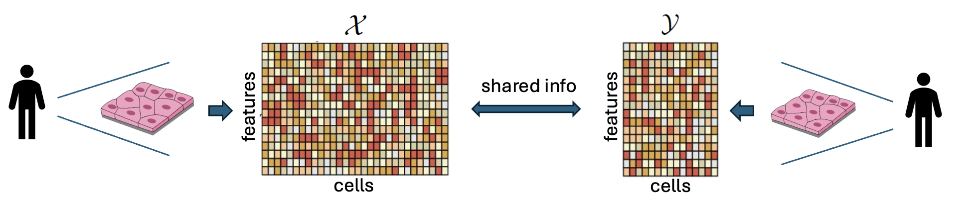
Figure 1: Illustration of multiple independently observed datasets with potentially shared information. Each dataset contains the same features but possibly different number of samples.

Motivated by these applications, this paper focuses on the joint embedding of two independently observed high-dimensional noisy datasets $\mathcal{X}=\{\mathbf{x}_{i}\}_{i=1}^{{n_{1}}}\subset\mathbb{R}^{p}$ and $\mathcal{Y}=\{\mathbf{y}_{j}\}_{j=1}^{n_{2}}\subset\mathbb{R}^{p},$ with possibly shared signal structures, as depicted in Figure 1. Our goal is to effectively learn the valuable signal structures from both datasets, which typically exhibit highly nonlinear patterns in biomedical research [44, 52]. Before proceeding further, we must first underscore the distinction between our concerned problem and a closely related yet markedly different problem which is also frequently encountered in modern biomedical research: the necessity of integrating datasets pertaining to identical samples, while each dataset comprising varying “views” or types of measurements [49, 33, 30]. For example, in single-cell multiomics research [2, 4], measurements on genomic variation and gene expression can be obtained simultaneously for the same set of cells, leading to two data matrices concerning distinct types (and numbers) of features [70]. The goal of multiomic analysis is to combine two or more views or modalities (e.g., genomic and transcriptomic information) of the same cells for more comprehensive profiling of their cell identities and associated molecular processes. The underlying analytical task is often known in literature as multi-view learning [71] or sensor fusion [21]. Lots of efforts are made to find effective algorithms under various assumptions, to list but a few, canonical correlation analysis (CCA) [24, 23], nonparametric canonical correlation analysis (NCCA) [42], kernel canonical correlation analysis (KCCA) [32], deep canonical correlation analysis (DCCA) [1], alternating diffusion [64], and time coupled diffusion maps [38], etc. For the sensor fusion problem, the two datasets, denoted as $\mathcal{X}^{\prime}=\{\mathbf{x}^{\prime}_{i}\}_{i=1}^{n}\subset\mathbb{R}^{p_{1}}$ and $\mathcal{Y}^{\prime}=\{\mathbf{y}^{\prime}_{j}\}_{j=1}^{n}\subset\mathbb{R}^{p_{2}}$, typically display dependence and possess an equal number of samples, $n$, yet they may differ in their feature dimensions, represented by $p_{1}$ and $p_{2}$, respectively. On the contrary, our work addresses a different problem where the two datasets $\mathcal{X}$ and $\mathcal{Y}$ are independent and share the same set of $p$ features, although they may possess varying sample sizes, $n_{1}$ and $n_{2}$.

Despite the importance and significance of the joint embedding problem in modern biomedical research, to our knowledge, it has not yet been formally or systematically addressed in the statistical literature. Several heuristic approaches have been developed specifically for single-cell applications; for example, see [22, 61, 8, 34, 29]. Despite their initial success, these existing works contain several fundamental limitations. First, all of these methods are developed heuristically and the absence of a theoretical foundation significantly constrains the users’ interpretation and exploitation of the datasets [35, 40, 45]. Second, existing methods are based on heuristics about clean signals in the low-dimensional setting so that their applicability and validity regarding high-dimensional and noisy datasets is in general left unguaranteed [35, 9]. Finally, biomedical datasets often exhibit high heterogeneity, characterized by varying signal-to-noise levels and sample sizes across individual datasets; however, existing methods do not provide automatic adaptation and oftentimes fail to effectively handle such information imbalance [37, 36].

To address these limitations, in this paper, we formulate this problem rigorously under a joint manifolds model framework (Assumption 3.1 and Figure 2) and propose a novel kernel spectral method that achieves joint embeddings of two independently observed high-dimensional and noisy datasets. Building upon the mathematical insights surrounding the newly introduced duo-landmark integral operators (Definition 3.4), we propose an asymmetric cross-data kernel matrix along with a data-adaptive bandwidth selection procedure (Algorithm 1) to capture the joint information contained in both datasets, and develop spectral joint embeddings of both datasets based on the singular values and singular vectors of the kernel matrix. The proposed method automatically captures and leverages possibly shared low-dimensional structures across datasets to enhance embedding quality. The obtained joint embeddings can be useful for many downstream tasks, such as simultaneous clustering (Section 4.1) and learning low-dimensional nonlinear structures (Section 4.2) on both datasets. The proposed method is justified by rigorous theoretical analysis, which guarantees consistency of the low-dimensional joint embeddings concerning the underlying signal structures, and provides explicit interpretations about its geometric meaning. When applied to real-world biological datasets (Section 5) – joint analysis of noisy and high-dimensional single-cell omics data – the proposed method demonstrates superior performance in capturing the underlying biological signals as compared with alternative methods.

1.2 Our algorithm, main results and contributions

Our proposed method is summarized in Algorithm 1. One remarkable feature is that it begins by connecting the data points from the point clouds $\mathcal{X}=\{\mathbf{x}_{i}\}_{1\leq i\leq n_{1}}\subset\mathbb{R}^{p}$ and $\mathcal{Y}=\{\mathbf{y}_{j}\}_{1\leq j\leq n_{2}},$ through the creation of an asymmetric rectangular kernel affinity matrix, as outlined in (2.2). As a result, we exclude “self-connections” within the individual point cloud $\mathcal{X}$ and $\mathcal{Y}$, focusing solely on connecting distinct data points between them. This approach is inspired and motivated by various theoretical and practical considerations as follows.

First, as mentioned in Section 1.1, our primary objective in practical applications is to effectively utilize both datasets and accomplish various downstream tasks simultaneously or separately. In this context, $\mathcal{X}$ and $\mathcal{Y}$ might only share partial information, limiting the relevance of self-connections within one dataset for understanding the structure of the other. This rationale also clarifies our decision not to amalgamate the two datasets and create a symmetric affinity matrix treating them as one entity, as the signal structures may not be entirely shared across both datasets. This is further confirmed by our simulations (Section 4) and analyses of real single-cell omics datasets (Section 5), which demonstrate that our approach significantly outperforms the methods that merely concatenate the two datasets and involve self-connections.

Second, from a theoretical standpoint, our approach draws significant inspiration from recent advancements in manifold learning that enhance the scalability of various algorithms through the utilization of landmark datasets [54, 55, 66, 69]. However, there exist significant differences between our aims and setups and theirs. For clarity, we focus on explaining the differences from [55]. In their configuration, only one set of cloud points is observed (let’s denote it as $\mathcal{X}$), with a single landmark dataset (let’s denote it as $\mathcal{Y}$), essentially resampled from $\mathcal{X}$. Consequently, the two point clouds are dependent. The remarkable contribution of [55] lies in providing guidance on selecting resampling schemes and resample sizes based on an analysis of a single differential operator, the Laplace operator. In contrast, as noted in Section 1.1, in our applications independent datasets $\mathcal{X}$ and $\mathcal{Y}$ are observed. In this context, $\mathcal{Y}$ can be considered the landmark dataset for $\mathcal{X}$, and conversely, $\mathcal{X}$ can also be viewed as the landmark dataset for $\mathcal{Y}$. This enables mutual learning between the two datasets through a pair of operators, namely, the newly introduced duo-landmark integral operators outlined in Definition 3.4. In both our theoretical analysis (Section 3) and numerical evaluations (Sections 4 and 5), the duo-landmark integral operators demonstrate the capacity to extract crucial structures from the underlying datasets with assistance from each other, despite only sharing partial common information.

Another important component in our Algorithm 1 is selecting an appropriate bandwidth parameter. Generalizing the approach from [16], our proposed method utilizes pairwise distances between datasets $\mathcal{X}$ and $\mathcal{Y}$, as described in (2.1). It is adaptive and does not depend on prior knowledge of the underlying data structures. Moreover, it theoretically ensures that our proposed joint embeddings (Step 3 of Algorithm 1) can be geometrically interpreted using the eigenfunctions of the duo-landmark integral operators.

In a manifold learning framework, we theoretically demonstrate that our proposed algorithm can produce embeddings capable of capturing the intrinsic structures of the underlying nonlinear manifolds, leveraging the eigenfunctions of the duo-integral operators linked with these manifolds. In our setup, shaped by the demands of our applications wherein datasets $\mathcal{X}$ and $\mathcal{Y}$ share only partial information, we propose a new joint manifolds model (Assumption 3.1 and Figure 2) for the underlying clean signals. The joint manifolds exhibit partially shared nonlinear structures, which can also be identical, thus encapsulating the common manifold model introduced in [17, 64] as a notable special case within our framework. For practical relevance, we consider the commonly used signal-plus-noise model for the observations where for $1\leq i\leq n_{1}$ and $1\leq j\leq n_{2}$

$$\mathbf{x}_{i}=\mathbf{x}_{i}^{0}+\bm{\xi}_{i}\in\mathbb{R}^{p},\qquad\mathbf{y}_{j}=\mathbf{y}_{j}^{0}+\bm{\zeta}_{j}\in\mathbb{R}^{p}.$$ (1.1)

where $\{\mathbf{x}_{i}^{0}\}$ and $\{\mathbf{y}_{j}^{0}\}$ are the clean signals in $\mathbb{R}^{p}$ sampled from the joint manifolds model and $\{\bm{\xi}_{i}\}$ and $\{\bm{\zeta}_{j}\}$ are the noise terms.

We emphasize that our approach allows the dimension $p$ to diverge alongside $n_{1}$ and $n_{2}$, addressing the issue of high dimensionality while also accommodating significant differences between $n_{1}$ and $n_{2}$. In essence, our methods are tailored to high-dimensional inputs, effectively mitigating potential imbalanced batch size effects. Moreover, we allow the signal strengths and signal-to-noise ratios (SNRs) to vary across different datasets, addressing the issue of information imbalance.

Under some mild conditions, we prove the convergence and robustness of our proposed algorithms. The theoretical novelty and significance can be summarized as follows.

• In the framework of the newly introduced joint manifolds model, we present a set of innovative integral operators known as duo-landmark integral operators (Definition 3.4). These operators encode the nonlinear manifold structures and are constructed upon convolution kernels alternating between the joint manifolds. This design facilitates the integration of information from datasets sampled from the two manifolds, enabling mutual learning between them.

• Under some mild conditions, we demonstrate the spectral convergence of our algorithms towards the duo-landmark operators. That is, when the datasets remain pristine (i.e., $\mathbf{x}_{i}=\mathbf{x}_{i}^{0}$ and $\mathbf{y}_{j}=\mathbf{y}_{j}^{0}$ in (1.1)), we establish that the outputs of our algorithms converge to the eigenvalues and eigenfunctions of the duo-landmark operators, accompanied by detailed convergence rate analyses.

• We also prove the robustness of our algorithm under the high-dimensional noise. We show that, under mild conditions on the SNRs, our proposed algorithm is robust to the noise and still converges to the duo-landmark integral operators. Consequently, our joint embeddings can be interpreted as a finite approximation of the samples projected onto the leading eigenfunctions of the duo-landmark integral operators.

Before concluding this section, it is worth noting that our algorithm can effectively handle a range of downstream tasks when the joint manifolds possess specific structures. For instance, in cases where both manifolds exhibit cluster structures, the joint embeddings will leverage the possibly shared cluster patterns, so that employing some clustering algorithms (e.g., k-means) simultaneously to the joint embeddings will lead to improved clustering of the datasets (Section 4.1). As another example, when the two datasets contain some partially shared nonlinear smooth manifold structures, but one has a higher SNR while the other has a lower SNR, the proposed joint embeddings would facilitate enhancing the embedding quality of the low-SNR dataset for better learning its underlying nonlinear manifolds (Section 4.2). In the applications to integrative single-cell omics analysis, we observe that compared with alternative methods, our algorithm achieves better performance in identifying the distinct cell types across heterogeneous datasets of gene expression or chromatin accessibility measures, generated from different experimental conditions or studies.

1.3 Organization and Notations

The rest of the paper is organized as follows. In Section 2, we introduce our proposed algorithm. In Section 3, we introduce the duo-landmark integral operators and prove the spectral convergence and robustness of our proposed methods. In Section 4, we use extensive numerical simulations to illustrate the usefulness of our method and in Section 5, we apply our algorithm to the integrative single-sell omics analysis. Some preliminary results are provided in Appendix A, the technical proofs of the main results are given in Appendix B and additional discussions on hyperparameter selection can be found in Appendix C.

We finish this section by introducing some notations. To streamline our statements, we use the notion of stochastic domination, which is commonly adopted in random matrix theory [20] to syntactically simplify precise statements of the form “$\mathsf{X}^{(n)}$ is bounded with high probability by $\mathsf{Y}^{(n)}$ up to small powers of $n$.”

Definition 1.1 (Stochastic domination).

Let $\mathsf{X}=\big{\{}\mathsf{X}^{(n)}(u):n\in\mathbb{N},\ u\in\mathsf{U}^{(n)}\big{\}}$ and $\mathsf{Y}=\big{\{}\mathsf{Y}^{(n)}(u):n\in\mathbb{N},\ u\in\mathsf{U}^{(n)}\big{\}}$ be two families of nonnegative random variables, where $\mathsf{U}^{(n)}$ is a possibly $n$-dependent parameter set. We say that $\mathsf{X}$ is stochastically dominated by $\mathsf{Y}$, uniformly in the parameter $u$, if for all small $\upsilon>0$ and large $D>0$, there exists $n_{0}(\upsilon,D)\in\mathbb{N}$ so that

$$\sup_{u\in\mathsf{U}^{(n)}}\mathbb{P}\Big{(}\mathsf{X}^{(n)}(u)>n^{\upsilon}\mathsf{Y}^{(n)}(u)\Big{)}\leq n^{-D},$$

for all $n\geq n_{0}(\upsilon,D)$. In addition, we say that an $n$-dependent event $\Omega\equiv\Omega(n)$ holds with high probability if for any large $D>1$, there exists $n_{0}=n_{0}(D)>0$ so that $\mathbb{P}(\Omega)\geq 1-n^{-D},$ for all $n\geq n_{0}.$

We interchangeably use the notation $\mathsf{X}=\mathrm{O}_{\prec}(\mathsf{Y})$, $\mathsf{X}\prec\mathsf{Y}$ or $\mathsf{Y}\succ\mathsf{X}$ if $\mathsf{X}$ is stochastically dominated by $\mathsf{Y}$, uniformly in $u\in\mathsf{U}^{(n)}$, when there is no risk of confusion. For two sequences of deterministic positive values $\{a_{n}\}$ and $\{b_{n}\},$ we write $a_{n}=\mathrm{O}(b_{n})$ if $a_{n}\leq Cb_{n}$ for some positive constant $C>0.$ In addition, if both $a_{n}=\mathrm{O}(b_{n})$ and $b_{n}=\mathrm{O}(a_{n}),$ we write $a_{n}\asymp b_{n}.$ Moreover, we write $a_{n}=\mathrm{o}(b_{n})$ if $a_{n}\leq c_{n}b_{n}$ for some positive sequence $c_{n}\to 0.$ For any probability measure $\mathsf{P}$ over $\Omega$, we denote $\mathcal{L}_{2}(\Omega,\mathsf{P})$ as the collection of $L_{2}$-integrable functions with respect to $\mathsf{P}$, that is, for any $f\in\mathcal{L}_{2}(\Omega,\mathsf{P})$, we have $\|f\|_{\mathsf{P}}=\sqrt{\int_{\Omega}|f(y)|^{2}\mathsf{P}(dy)}<\infty$. For a vector $\mathbb{a}=(a_{1},...,a_{n})^{\top}\in\mathbb{R}^{n}$, we define its $\ell_{p}$ norm as $\|\mathbb{a}\|_{p}=\big{(}\sum_{i=1}^{n}|a_{i}|^{p}\big{)}^{1/p}$. We denote $\text{diag}(a_{1},...,a_{n})\in\mathbb{R}^{n\times n}$ as the diagonal matrix whose $i$-th diagonal entry is $a_{i}$. For a matrix $\mathbb{A}=(a_{ij})\in\mathbb{R}^{n\times n}$, we define its Frobenius norm as $\|\mathbb{A}\|_{F}=\sqrt{\sum_{i=1}^{n}\sum_{j=1}^{n}a^{2}_{ij}}$, and its operator norm as $\|\mathbb{A}\|=\sup_{\|\mathbb{x}\|_{2}\leq 1}\|\mathbb{A}\mathbb{x}\|_{2}$. For any integer $n>0$, we denote the set $[n]=\{1,2,...,n\}$. For a random vector $\mathbf{g},$ we say it is sub-Gaussian if $\mathbb{E}\exp(\mathbf{a}^{\top}\mathbf{g})\leq\exp\left(\|\mathbf{a}\|_{2}^{2}/2\right)$ for any deterministic vector $\mathbf{a}.$ Throughout, $C,C_{1},C_{2},...$ are universal constants independent of $n$, and can vary from line to line. We denote ${\bf I}_{n}$ as an $n$-dimensional identity matrix.

2 Proposed algorithm

In this section, we introduce our new algorithm for the joint embedding of two datasets with the same features, summarized below in Algorithm 1.

Algorithm 1 Kernel spectral joint embeddings using duo-landmark integral operator

Input: Observed (centered) samples $\{\mathbf{x}_{j}\}_{j\in[n_{1}]}$, $\{\mathbf{y}_{i}\}_{i\in[n_{2}]}$, percentile $\omega\in(0,1)$ and singular vector index sets $\Omega_{1}\subseteq\{1,2,...,n_{1}\}$ and $\Omega_{2}\subseteq\{1,2,...,n_{2}\}$.

1. Bandwidth selection:

     (i) let $d_{ij}=\|\mathbf{x}_{i}-\mathbf{y}_{j}\|_{2}^{2}$ for all $1\leq i\leq n_{1}$ and $1\leq j\leq n_{2}$, and define the empirical cumulative distribution function

$$\nu_{n}(t)=\frac{1}{n_{1}n_{2}}\sum_{\begin{subarray}{c}1\leq i\leq n_{1}\\ 1\leq j\leq n_{2}\end{subarray}}1_{\{d_{ij}\leq t\}},$$

     (ii) define the bandwidth $h_{n}$ to be the solution to the equation

$$\nu_{n}(h_{n})=\omega.$$ (2.1)

2. Kernel matrix construction: define the kernel matrix $\mathbb{K}:=(K(i,j))\in\mathbb{R}^{n_{1}\times n_{2}}$ using the above bandwidth $h_{n}$ by letting

$$K(i,j)=\exp\bigg{(}-\frac{\|\mathbf{x}_{i}-\mathbf{y}_{j}\|_{2}^{2}}{h_{n}}\bigg{)}.$$ (2.2)

3. Obtain joint embeddings:

     (i) obtain the singular value decomposition (SVD) of the scaled kernel matrix $(n_{1}n_{2})^{-1}\mathbb{K}$ as

$$\frac{1}{n_{1}n_{2}}\mathbb{K}=\sum_{i=1}^{\min\{n_{1},n_{2}\}}s_{i}\mathbf{u}_{i}\mathbf{v}_{i}^{\top},$$ (2.3)

where $s_{1}\geq s_{2}\geq...\geq s_{\min\{n_{1},n_{2}\}}$ being the singular values of $(n_{1}n_{2})^{-1}\mathbb{K}$, and $\{\mathbf{u}_{i}\}$ and $\{\mathbf{v}_{i}\}$ being the corresponding left and right singular vectors.

     (ii) let $\mathbb{U}_{\Omega_{1}}\in\mathbb{R}^{n_{1}\times|\Omega_{1}|}$ contain the left singular vectors indexed by the elements in $\Omega_{1}$, $\mathbb{V}_{\Omega_{2}}\in\mathbb{R}^{n_{2}\times|\Omega_{2}|}$ contain the right singular vectors indexed by the elements in $\Omega_{2}.$ Moreover, let $\Lambda_{\Omega_{1(2)}}$ be a $|\Omega_{1(2)}|\times|\Omega_{1(2)}|$ diagonal matrix containing the singular values indexed by the elements in $\Omega_{1(2)}.$

Output: the kernel embedding matrices for $\{\mathbf{x}_{i}\}$ and $\{\mathbf{y}_{i}\}$ are $\mathbb{U}_{\Omega_{1}}\Lambda_{\Omega_{1}}$ and $\mathbb{V}_{\Omega_{2}}\Lambda_{\Omega_{2}},$ respectively.

In Step 1 of the algorithm, a data-adaptive bandwidth parameter $h_{n}$ is chosen as the $\omega$-percentile of the empirical cumulative distribution function $\nu_{n}(t)$ of the pairwise between-dataset squared-distances $\{d_{ij}\}_{1\leq i\leq n_{1},1\leq j\leq n_{2}}\equiv\{\|\mathbf{x}_{i}-\mathbf{y}_{j}\|_{2}^{2}\}_{1\leq i\leq n_{1},1\leq j\leq n_{2}}$ of the observed datasets. Such a strategy is motivated by our theoretical analysis of the spectrum of kernel random matrices and its dependence on the associated bandwidth parameter; see Proposition A.8. It ensures the thus determined bandwidth $h_{n}$ adapts well to the unknown nonlinear structures and the SNRs of the datasets, so that the singular values and singular vectors of the associated kernel matrix capture the respective underlying low-dimensional structures via the duo-landmark integral operators; see Section 3 for more details. The percentile $\omega$ is a tunable hyperparameter. In Section 3, we show in theory $\omega$ can be chosen as any constant between 0 and 1 to have the final embeddings achieve the same asymptotic behavior. In practice, to optimize the empirical performance and improve automation of the method, we recommend using a resampling approach as in [16, 12], described in Appendix C, to determine the percentile $\omega$. In Step 2, we construct the kernel matrix $\mathbb{K}=(K(i,j))\in\mathbb{R}^{n_{1}\times n_{2}}$, $K(i,j)=\exp(-{d_{ij}}/{h_{n}})$, using the distances of the data points solely between the two datasets. Notably, the kernel matrix $\mathbb{K}$ is of dimension $n_{1}\times n_{2}$ and rectangular in general. For simplicity, here we focus on the Gaussian kernel function. The results can be extended to other positive definite kernels as in [14]; see Remark 3.14 for more details. In Step 3, the final embeddings are defined as the $(\Omega_{1},\Omega_{2})$-indexed leading left and right singular vectors of the scaled kernel matrix, weighted by their respective singular values. The index sets $\Omega_{1}$ and $\Omega_{2}$ of the embedding space are determined by the users, depending on the specific aims or downstream applications of the low-dimensional embeddings.

In the next section, we discuss in detail the theoretical properties of the proposed algorithm, which justify its robust performance when applied to high-dimensional noisy datasets, and provide a rigorous geometric interpretation of the final joint embeddings.

3 Theoretical analysis

We follow and generalize [14, 16, 19] and assume that $\{\mathbf{x}_{i}\}$ and $\{\mathbf{y}_{j}\}$ are sampled from some nonlinear manifolds model and corrupted by high-dimensional noise as in (1.1). In what follows, we introduce the nonlinear manifolds model and the duo-landmark integral operators in Section 3.1. In Section 3.2, we establish the convergence results of $(n_{1}n_{2})^{-1}\mathbb{K}^{0}$ to the duo-landmark integral operators, where $\mathbb{K}^{0}$ is defined similarly as in (2.2) but using the clean signals, that is,

$$\mathbb{K}^{0}=(K^{0}(i,j)),\qquad K^{0}(i,j)=\exp\left(-\frac{\|\mathbf{x}_{i}^{0}-\mathbf{y}_{j}^{0}\|_{2}^{2}}{h^{0}_{n}}\right),$$ (3.1)

where $h_{n}^{0}$ is defined in the same way as in (2.1) using the clean signals. In Section 3.3, we show that our proposed algorithm is robust to high-dimensional noise.

3.1 Joint manifolds model and duo-landmark integral operators

For the clean signals $\{\mathbf{x}_{i}^{0}\}$ and $\{\mathbf{y}_{j}^{0}\}$, we suppose that they are sampled from some smooth manifolds model, which generalizes those considered in [10, 64, 67], and is formally summarized in Assumption 3.1. Since our Algorithm 1 concerns datasets after centralization, without loss of generality, we can assume that all the samples are centered.

Assumption 3.1.

For $\mathbf{x}_{i}^{0},1\leq i\leq n_{1},$ we assume that they are centered and i.i.d. sampled from some sub-Gaussian random vector $X:\Omega_{1}\rightarrow\mathbb{R}^{p}$ with respect to some probability space $(\Omega_{1},\mathcal{F}_{1},\mathbb{P}_{1}).$ Moreover, we assume that the range of $X$ is supported on an $m_{1}$-dimensional connected Riemannian manifold $\mathcal{M}_{1}$ isometrically embedded in $\mathbb{R}^{p}$ via $\iota_{1}:\mathcal{M}_{1}\rightarrow\mathbb{R}^{p}.$ We suppose that $\operatorname{dim}(\iota_{1}(\mathcal{M}_{1}))=r_{1}\leq p.$ Let $\widetilde{\mathcal{F}}_{1}$ be the Borel sigma algebra of $\iota_{1}(\mathcal{M}_{1})$ and denotes $\widetilde{\mathbb{P}}_{1}$ be the probability measure of $X$ defined on $\widetilde{\mathcal{F}}_{1}$ induced from $\mathbb{P}_{1}.$ We assume that $\widetilde{\mathbb{P}}_{1}$ is absolutely continuous with respect to the volume measure on $\iota_{1}(\mathcal{M}_{1})$ whose density function is strictly positive. In addition, we assume that similar conditions hold for $\mathbf{y}_{j},1\leq j\leq n_{2},$ by replacing the quantities $(\Omega_{1},\mathcal{F}_{1},\mathbb{P}_{1},X,\mathcal{M}_{1},\iota_{1},r_{1})$ by some other combinations $(\Omega_{2},\mathcal{F}_{2},\mathbb{P}_{2},Y,\mathcal{M}_{2},\iota_{2},r_{2}).$ Finally, we assume that $\{\mathbf{x}_{i}^{0}\}$ and $\{\mathbf{y}_{j}^{0}\}$ are independent. We shall call the above model as the joint manifolds model and an illustration is given in Figure 2 below.

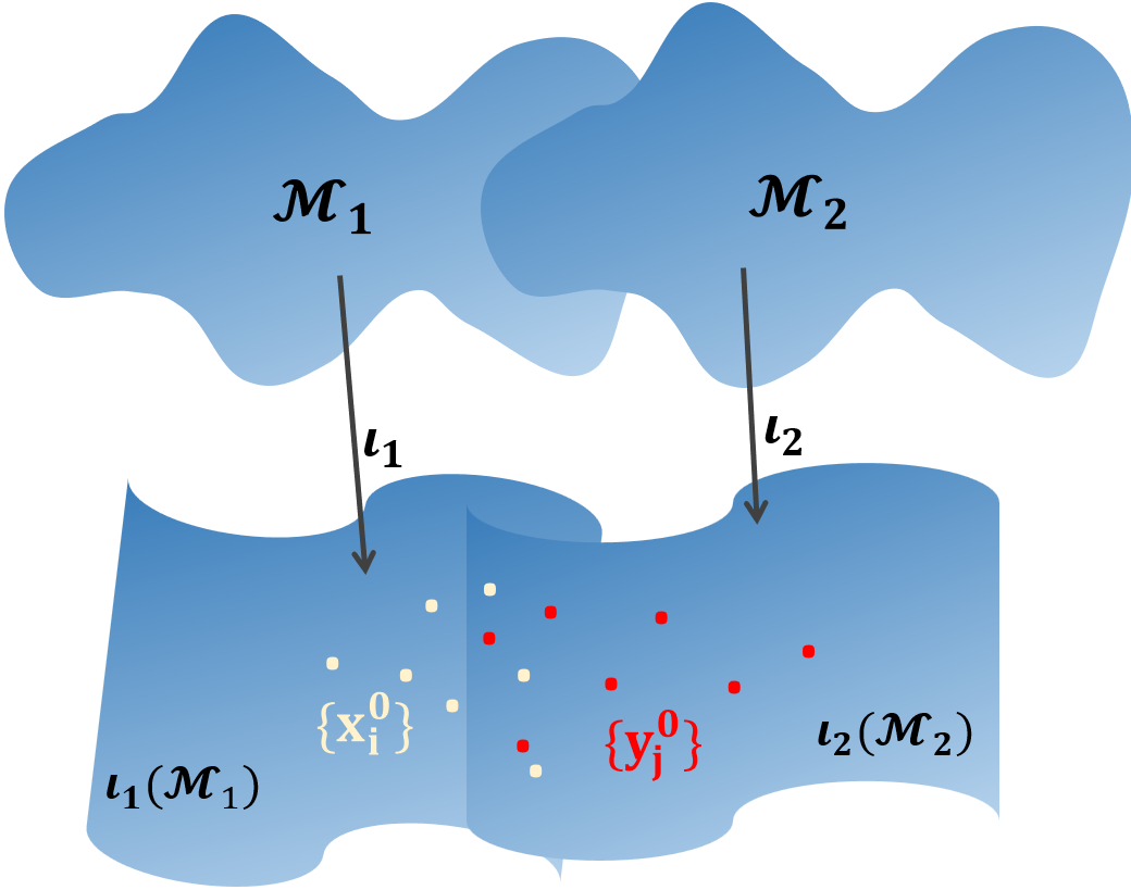
Figure 2: Illustration of the joint manifolds model. Here $\iota_{1}(\mathcal{M}_{1})$ and $\iota_{2}(\mathcal{M}_{2})$ may contain partially overlapped or identical structures. This generalizes the common manifold model considered in [17, 64].

Before proceeding to introduce the duo-landmark integral operators, we introduce a model reduction scheme which largely generalizes the framework proposed in [16]. Let

$$\operatorname{Cov}(X)=\mathbb{\Sigma}_{1},\qquad\operatorname{Cov}(Y)=\mathbb{\Sigma}_{2}.$$ (3.2)

Due to independence, we have that for $Z=X-Y,$

$$\operatorname{Cov}(Z):=\mathbb{\Sigma}=\mathbb{\Sigma}_{1}+\mathbb{\Sigma}_{2}.$$

For the rank $r=\operatorname{rank}(\mathbb{\Sigma}),$ it is clear that $\max\{r_{1},r_{2}\}\leq r\leq r_{1}+r_{2}.$ Similar to the discussions in Appendix A.2 of [16], there exists a rotation matrix $\mathbb{R}$ so that

$$\mathbb{R}Z=(Z_{1},Z_{2},\cdots,Z_{r},0,\cdots,0).$$

Let the spectral decomposition of $\operatorname{Cov}(Z_{1},\cdots,Z_{r})$ be $\mathbb{\Sigma}_{r}=\mathbb{V}\mathbb{\Theta}\mathbb{V}^{\top},$ where $\mathbb{\Theta}=\operatorname{diag}(\theta_{1},\cdots,\theta_{r})$ is a diagonal matrix of the eigenvalues and $\mathbb{V}$ contains the eigenvectors as its columns. For the orthogonal matrix $\mathbb{O}\in\mathbb{R}^{p\times p}$ given by

$$\mathbb{O}=\begin{bmatrix}\mathbb{V}^{\top}&{\bf 0}\\ {\bf 0}&{\bf I}_{p-r}\end{bmatrix},$$

we see that

$$\text{Cov}(\mathbb{O}\mathbb{R}Z)=\begin{bmatrix}\mathbb{\Theta}&{\bf 0}\\ {\bf 0}&{\bf 0}\end{bmatrix}.$$

Based on the above discussion, since Euclidean distance is invariant to rotations, for (3.1), we have

$$\exp\bigg{(}-\frac{\|\mathbf{x}^{0}_{i}-\mathbf{y}^{0}_{j}\|_{2}^{2}}{h^{0}_{n}}\bigg{)}=\exp\bigg{(}-\frac{\|\mathbb{O}\mathbb{R}\mathbf{x}^{0}_{i}-\mathbb{O}\mathbb{R}\mathbf{y}^{0}_{j}\|_{2}^{2}}{h^{0}_{n}}\bigg{)}.$$

Consequently, without loss of generality, we can directly use $\mathbb{O}\mathbb{R}\mathbf{x}^{0}_{i}-\mathbb{O}\mathbb{R}\mathbf{y}^{0}_{j}$ and focus on

$$\mathbf{z}^{0}_{ij}:=\mathbb{O}\mathbb{R}(\mathbf{x}_{i}^{0}-\mathbf{y}^{0}_{j})=(z_{ij,1},\cdots,z_{ij,r},\mathbf{0}),$$ (3.3)

with

$$\operatorname{Cov}(z_{ij,1},\cdots,z_{ij,r})=\operatorname{diag}(\theta_{1},\cdots,\theta_{r}).$$ (3.4)

Denote the sets

$$\mathcal{S}_{1}=\left\{\mathbb{O}\mathbb{R}\mathbf{x}^{0}:\ \mathbf{x}^{0}\in\iota_{1}(\mathcal{M}_{1})\right\},\qquad\mathcal{S}_{2}=\left\{\mathbb{O}\mathbb{R}\mathbf{y}^{0}:\ \mathbf{y}^{0}\in\iota_{2}(\mathcal{M}_{2})\right\}.$$ (3.5)

Moreover, we define the probability measure on $\mathcal{S}_{1}$ for $\mathbb{O}\mathbb{R}X$ based on $\widetilde{\mathbb{P}}_{1}$ as $\widetilde{\mathsf{P}}_{1}.$ Similarly, the measure on $\mathcal{S}_{2}$ for $\mathbb{O}\mathbb{R}Y$ based on $\widetilde{\mathbb{P}}_{2}$ as $\widetilde{\mathsf{P}}_{2}.$

Next we introduce the duo-landmark integral operators for the reduced model (3.3) on the sets (3.5), inspired by the works [54, 55]. For notional simplicity, we set that for $\bm{x},\bm{y}\in\mathbb{R}^{p}$

$$k(\bm{x},\bm{y})=\exp\left(-\frac{\|\bm{x}-\bm{y}\|_{2}^{2}}{h^{0}_{n}}\right).$$ (3.6)

Based on the kernel in (3.6) and the joint manifolds model in Assumption 3.1, we now define two new kernel functions as follows.

Definition 3.2 (Convolutional landmark kernels).

For $\bm{x}_{1},\bm{x}_{2}\in\mathcal{S}_{1},$ we define the kernel $k_{1}(\cdot,\cdot):\mathcal{S}_{1}\times\mathcal{S}_{1}\rightarrow\mathbb{R}$ as follows

$$k_{1}(\bm{x}_{1},\bm{x}_{2})=\int_{\mathcal{S}_{2}}k(\bm{x}_{1},\bm{z})k(\bm{z},\bm{x}_{2})\widetilde{\mathsf{P}}_{2}(\mathrm{d}\bm{z}).$$ (3.7)

Similarly, for $\bm{y}_{1},\bm{y}_{2}\in\mathcal{S}_{2},$ we define the kernel $k_{2}(\cdot,\cdot):\mathcal{S}_{2}\times\mathcal{S}_{2}\rightarrow\mathbb{R}$ as follows

$$k_{2}(\bm{y}_{1},\bm{y}_{2})=\int_{\mathcal{S}_{1}}k(\bm{y}_{1},\bm{z})k(\bm{z},\bm{y}_{2})\widetilde{\mathsf{P}}_{1}(\mathrm{d}\bm{z}).$$ (3.8)

We shall call the kernels $k_{1}(\cdot,\cdot)$ and $k_{2}(\cdot,\cdot)$ the convolutional landmark kernels.

Note that $k_{1}(\cdot,\cdot)$ can be understood as a convolution of two kernels using $\iota_{2}(\mathcal{M}_{2})$ as a landmark population. Similar discussion applies to $k_{2}(\cdot,\cdot).$ The following proposition shows that both kernels in (3.7) and (3.8) are positive definite so that the integral operators and reproducing kernel Hilbert spaces (RKHSs; see Appendix A.1 for some background) can be constructed based on them accordingly.

Proposition 3.3.

Suppose Assumption 3.1 hold. Then the kernels in Definition 3.2 are bounded and positive definite.

Proof.

See Section B.2. ∎

Based on Proposition 3.3, we now introduce the duo-landmark integral operators.

Definition 3.4 (Duo-landmark integral operators).

Let $\mathcal{K}_{1}$ and $\mathcal{K}_{2}$ be operators defined on $\mathcal{L}_{2}(\mathcal{S}_{1},\widetilde{\mathsf{P}}_{1})$ and $\mathcal{L}_{2}(\mathcal{S}_{2},\widetilde{\mathsf{P}}_{2}),$ respectively. For $\ell=1,2$ and $g_{\ell}\in\mathcal{L}_{2}(\mathcal{S}_{\ell},\widetilde{\mathsf{P}}_{\ell}),$ we define the duo-landmark integral operators $(\mathcal{K}_{1},\mathcal{K}_{2})$ as follows

$$\mathcal{K}_{\ell}g_{\ell}(\bm{z})=\int_{\mathcal{S}_{\ell}}k_{\ell}(\bm{z},\bm{y})g_{\ell}(\bm{y})\widetilde{\mathsf{P}}_{\ell}(\mathrm{d}\bm{y}),\qquad\ell=1,2.$$

Remark 3.5.

Since $k(\cdot,\cdot)$ in (3.6) is a positive-define kernel, it is well-known from [53] that $\mathcal{L}_{2}(\mathcal{S}_{1},\widetilde{\mathsf{P}}_{1})$ and $\mathcal{L}_{2}(\mathcal{S}_{2},\widetilde{\mathsf{P}}_{2})$ equipped with the kernel (3.6) can be made into two RKHSs, respectively, denoted as $\mathcal{H}_{1}$ and $\mathcal{H}_{2}$. In addition, the two RKHSs are closely related to two other integral operators $\mathcal{G}_{\ell},\ell=1,2,$ given by

$$\mathcal{G}_{\ell}g_{\ell}(\bm{x})=\int_{\mathcal{S}_{\ell}}k(\bm{x},\bm{y})g_{\ell}(\bm{y})\widetilde{\mathsf{P}}_{\ell}(\mathrm{d}\bm{y}),\qquad g_{\ell}\in\mathcal{L}_{2}(\mathcal{S}_{\ell},\widetilde{\mathsf{P}}_{\ell}).$$ (3.9)

Furthermore, $k(\cdot,\cdot)$ can be decomposed using Mercer’s theorem (see Theorem 2.10 of [53]) in the sense that for $\ell=1,2,$

$$k(\bm{x},\bm{y})=\sum_{j}\lambda^{\ell}_{j}\psi_{j}^{\ell}(\bm{x})\psi_{j}^{\ell}(\bm{y}),$$

where $\{\lambda_{j}^{\ell}\}$ and $\{\psi_{j}^{\ell}(\cdot)\}$ are the eigenvalues and eigenfunctions of the integral operators $\mathcal{G}_{\ell}$ in (3.9).

Similarly, as in Definition 3.4, one can also build RKHSs using the kernels (3.7) and (3.8) on $\mathcal{L}_{2}(\mathcal{S}_{1},\widetilde{\mathsf{P}}_{1})$ and $\mathcal{L}_{2}(\mathcal{S}_{2},\widetilde{\mathsf{P}}_{2}).$ Using Mercer’s theorem, one can also expand the kernels $k_{1}(\cdot,\cdot)$ and $k_{2}(\cdot,\cdot).$ As can be seen in the proof of Proposition 3.3, in the expansions of $k_{1}(\cdot,\cdot),$ the eigenvalues and eigefunctions are closely related to those of the operator $\mathcal{G}_{2}$ in (3.9), while $k_{2}$ is closely related to $\mathcal{G}_{1};$ see (B.2) for more precise statements. From the above discussion, we can see the difference between using the operators $\mathcal{G}_{\ell},\ell=1,2,$ in (3.9) and $\mathcal{K}_{\ell},\ell=1,2,$ in Definition 3.4. The former operators only utilize the information from one dataset whereas the later operators aim at integrating the information from two datasets. As we will see later, these operators can provide more useful information about the datasets.

Finally, we point out that in (3.6) and the constructions in Definition 3.2, for simplicity we use the Gaussian kernel. However, we can easily generalize our results for a large class of kernel functions. For more details, we refer the readers to Remark 3.14.

3.2 Spectral convergence analysis

In this section, we show that when both datasets are clean signals (i.e., $\mathbf{x}_{i}=\mathbf{x}_{i}^{0}$ and $\mathbf{y}_{j}=\mathbf{y}_{j}^{0}$ in (1.1)), the embeddings obtained from Algorithm 1 have close relations with the eigenfunctions of the operators $\mathcal{K}_{1}$ and $\mathcal{K}_{2}$ in Definition 3.4. More specifically, the singular values and vectors of the matrix $\mathbb{K}^{0}$ in (3.1) are closely related to the eigenvalues and eigenfunctions of the operators $\mathcal{K}_{1}$ and $\mathcal{K}_{2}.$ Before stating our main results, we first provide an important result on the eigenvalues of the operators. Recall that $\mathcal{H}_{1}$ and $\mathcal{H}_{2}$ are the RKHSs built on $\mathcal{L}_{2}(\mathcal{S}_{1},\widetilde{\mathsf{P}}_{1})$ and $\mathcal{L}_{2}(\mathcal{S}_{2},\widetilde{\mathsf{P}}_{2})$ separately using the kernel (3.6).

Proposition 3.6.

Suppose Assumption 3.1 holds. Moreover, we assume that there exists some common measurable space $\mathcal{N}\subset\mathbb{R}^{p}$ that $\mathcal{H}_{i},i=1,2,$ are compactly embedded into $\mathcal{L}_{2}(\mathcal{N},\widetilde{\mathsf{P}}_{i}).$ Then we have that operators $\mathcal{K}_{1}$ and $\mathcal{K}_{2}$ have the same set of nonzero eigenvalues.

Proof.

See Section B.3. ∎

Remark 3.7.

We provide two remarks on Proposition 3.6. First, our proposed Algorithm 1 provides the joint embeddings by using the singular values and vectors of the matrix in (2.3). Therefore, if the two embeddings are associated with some operators, it is necessary that these two operators must share the same nonzero eigenvalues. In this sense, Proposition 3.6 is the basis of our theoretical analysis. Second, the assumption that $\mathcal{H}_{i},i=1,2,$ are compactly embedded into the $\mathcal{L}_{2}$ spaces is a mild assumption and used frequently in the literature, for example, see [25, 41, 60]. It guarantees that the orthonormal basis of the RKHSs and the $\mathcal{L}_{2}$ spaces are closely related; see Lemma A.3 for more precise statements. Roughly speaking, it requires that the two manifolds in Assumption 3.9 have common structures so that the RKHSs built on them share common information.

Based on Proposition 3.6, we denote $\{\gamma_{i}\}$ as the nonzero eigenvalues of $\mathcal{K}_{1}$ and $\mathcal{K}_{2}$ in the decreasing order. Moreover, we denote $\{\phi_{i}(\bm{x})\}$ and $\{\psi_{i}(\bm{y})\}$ as the eigenfunctions of $\mathcal{K}_{1}$ and $\mathcal{K}_{2},$ respectively. That is for $\bm{x}\in\mathcal{S}_{1}$ and $\bm{y}\in\mathcal{S}_{2}$

$$\mathcal{K}_{1}\phi_{i}(\bm{x})=\gamma_{i}\phi_{i}(\bm{x}),\quad\ \mathcal{K}_{2}\psi_{i}(\bm{y})=\gamma_{i}\psi_{i}(\bm{y}).$$ (3.10)

Moreover, for $\mathbb{K}^{0}=(K^{0}(i,j))$ defined in (3.1), we denote

$$\mathbb{N}_{01}=\frac{1}{n_{1}n_{2}}\mathbb{K}^{0}(\mathbb{K}^{0})^{\top},\quad\mathbb{N}_{02}=\frac{1}{n_{2}n_{1}}(\mathbb{K}^{0})^{\top}\mathbb{K}^{0}.$$ (3.11)

It is clear that $\mathbb{N}_{01}$ and $\mathbb{N}_{02}$ share the same nonzero eigenvalues. We denote them as $\{\lambda_{i}\}.$ Moreover, we denote the associated eigenvectors of $\mathbb{N}_{01}$ and $\mathbb{N}_{02}$ as $\{\mathbb{u}_{i}^{0}\}$ and $\{\mathbb{v}_{i}^{0}\},$ respectively. As such, $\{\lambda^{1/2}_{i}\}$ are the nonzero singular values of $(n_{1}n_{2})^{-1/2}\mathbb{K}^{0}$, whereas $\{\mathbb{u}_{i}^{0}\}$ and $\{\mathbb{v}_{i}^{0}\}$ are the left and right singular vectors of $(n_{1}n_{2})^{-1/2}\mathbb{K}^{0}.$ To better describe the convergence of $\{\mathbb{u}_{i}^{0}\}$ and $\{\mathbb{v}_{i}^{0}\}$, for the kernel function defined in (3.6), we further denote

$$\widehat{k}^{0}_{1}(\bm{x}_{1},\bm{x}_{2})=\frac{1}{n_{2}}\sum_{s=1}^{n_{2}}k(\bm{x}_{1},\mathbf{y}^{0}_{s})k(\mathbf{y}^{0}_{s},\bm{x}_{2}),\qquad\widehat{k}^{0}_{2}(\bm{y}_{1},\bm{y}_{2})=\frac{1}{n_{1}}\sum_{s=1}^{n_{1}}k(\bm{y}_{1},\mathbf{x}^{0}_{s})k(\mathbf{x}^{0}_{s},\bm{y}_{2}).$$ (3.12)

and define the functions

$$\widehat{\phi}^{0}_{i}(\bm{x})=\frac{1}{\lambda_{i}\sqrt{n_{1}}}\sum_{j=1}^{n_{1}}\widehat{k}^{0}_{1}(\bm{x},\mathbf{x}^{0}_{j})u^{0}_{ij},\qquad\widehat{\psi}^{0}_{i}(\bm{y})=\frac{1}{\lambda_{i}\sqrt{n_{2}}}\sum_{j=1}^{n_{2}}\widehat{k}^{0}_{2}(\bm{y},\mathbf{y}^{0}_{j})v^{0}_{ij},$$ (3.13)

where $\mathbf{u}^{0}_{i}=(u^{0}_{i1},\cdots,u^{0}_{in_{1}})^{\top}$ and $\mathbf{v}^{0}_{i}=(v^{0}_{i1},\cdots,v^{0}_{in_{2}})^{\top}.$ Note that by the above construction, we have that

$$\widehat{\phi}^{0}_{i}(\mathbf{x}^{0}_{j})=\sqrt{n_{1}}u^{0}_{ij},\qquad\widehat{\psi}^{0}_{i}(\mathbf{y}^{0}_{j})=\sqrt{n_{2}}v^{0}_{ij}.$$

Armed with the above notations, we proceed to state our results. In what follows, we always assume that $\gamma_{1}\geq\gamma_{2}\geq\cdots,$ are sorted in a decreasing fashion. Similarly, for $\{\lambda_{i}\}.$ For some constant $\delta>0,$ we define

$$\mathsf{K}\equiv\mathsf{K}(\delta):=\operatorname{arg\ max}\left\{i:\gamma_{i}\geq\delta\right\},$$ (3.14)

and for all $1\leq i\leq\mathsf{K}$

$$\mathsf{r}_{i}=\min\{\gamma_{i-1}-\gamma_{i},\gamma_{i}-\gamma_{i+1}\}.$$ (3.15)

Theorem 3.8.

Suppose the assumptions of Proposition 3.6 hold. Then we have that when $n_{1}$ and $n_{2}$ are sufficiently large,

$$\sup_{i}|\lambda_{i}-\gamma_{i}|\prec n_{1}^{-1/2}+n_{2}^{-1/2}.$$ (3.16)

Moreover, for each $1\leq i\leq\mathsf{K}$ and $\mathsf{r}_{i}$ in (3.15) satisfying that for some small constant $\tau>0$

$$n_{1}^{-1/2+\tau}+n_{2}^{-1/2+\tau}=\mathrm{o}(\mathsf{r}_{i}),$$ (3.17)

we have that, for any $\bm{x}\in\mathcal{S}_{1}$

$$|\sqrt{\gamma_{i}}{\phi}_{i}(\bm{x})-\sqrt{\lambda_{i}}\widehat{\phi}^{0}_{i}(\bm{x})|\prec\frac{1}{\mathsf{r}_{i}}\bigg{(}\frac{1}{\sqrt{n_{1}}}+\frac{1}{\sqrt{n_{2}}}\bigg{)}+\frac{1}{\sqrt{n_{2}}},$$ (3.18)

and for any $\bm{y}\in\mathcal{S}_{2}$,

$$|\sqrt{\gamma_{i}}{\psi}_{i}(\bm{y})-\sqrt{\lambda_{i}}\widehat{\psi}^{0}_{i}(\bm{y})|\prec\frac{1}{\mathsf{r}_{i}}\bigg{(}\frac{1}{\sqrt{n_{1}}}+\frac{1}{\sqrt{n_{2}}}\bigg{)}+\frac{1}{\sqrt{n_{1}}},$$

where $\mathcal{S}_{1}$ and $\mathcal{S}_{2}$ are defined in (3.5).

Proof.

See Section B.3. ∎

We provide several remarks. First, Theorem 3.8 establishes the spectral convergence results of the matrices in (3.11) to the duo-landmark integral operators in Definition 3.4 under the clean signals. We now explain the high-level heuristics using the embeddings for $\{\mathbf{x}_{i}^{0}\}$ as an example. Note that for all $1\leq i,j\leq n_{1},$ by law of large number, roughly speaking, we have that for the kernel in (3.7)

$$n_{1}(\mathbb{N}_{01})_{ij} =\frac{1}{n_{2}}(\mathbb{K}^{0}(\mathbb{K}^{0})^{\top})_{ij}=\frac{1}{n_{2}}\sum_{s=1}^{n_{2}}k(\mathbf{x}^{0}_{i},\mathbf{y}^{0}_{s})k(\mathbf{y}^{0}_{s},\mathbf{x}^{0}_{j})$$

$$\approx\int_{\mathcal{S}_{2}}k(\mathbf{x}_{i}^{0},\bm{z})k(\bm{z},\mathbf{x}_{j}^{0})\widetilde{\mathsf{P}}_{2}(\mathrm{d}\bm{z})\equiv k_{1}(\mathbf{x}_{i}^{0},\mathbf{x}_{j}^{0}).$$ (3.19)

Consequently, if one defines $\mathbb{W}_{01}=(W_{01}(i,j))\in\mathbb{R}^{n_{1}\times n_{1}}$ with $W_{01}(i,j)=k_{1}(\mathbf{x}_{i}^{0},\mathbf{x}_{j}^{0}),$ similar to the argument in [31, 51], one can see that $n_{1}^{-1}\mathbb{W}_{01}$ will be closely related to the operator $\mathcal{K}_{1}$ defined via the kernel $k_{1}$ in (3.7). This explains the closeness between the matrix $\mathbb{N}_{01}$ in (3.11) and the operator $\mathcal{K}_{1}.$ It is worth pointing out that the scaling $n_{2}^{-1}$ is needed for the convergence of the convolution part in (3.2) whereas $n_{1}^{-1}$ is related to the dimension of $\mathbb{W}_{01}$, essentially ensuring the convergence of $\mathbb{W}_{01}.$

Second, we provide some insights on the differences in constructing embeddings between only using a single dataset and with the help of the landmark dataset. We use the dataset $\{\mathbf{x}_{i}^{0}\}$ as an example. Note that after some simple algebraic manipulation, one can rewrite (3.2) as follows

$$k_{1}(\mathbf{x}_{i}^{0},\mathbf{x}_{j}^{0})=\mathsf{g}(\mathbf{x}^{0}_{i},\mathbf{x}^{0}_{j},\{\mathbf{y}_{i}^{0}\})k(\mathbf{x}_{i}^{0},\mathbf{x}_{j}^{0}),$$

for some function $\mathsf{g}.$ On the one hand, when one only uses the single dataset $\{\mathbf{x}_{i}^{0}\}$, it is easy to see that $\mathsf{g}\equiv 1$ so that $\mathbf{x}_{i}^{0}$ and $\mathbf{x}_{j}^{0}$ are connected using the kernel $k.$ On the other hand, our proposed algorithm utilizes both $\{\mathbf{x}_{i}^{0}\}$ and the landmark dataset $\{\mathbf{y}_{i}^{0}\}$ so that $\mathbf{x}_{i}^{0}$ and $\mathbf{x}_{j}^{0}$ will be connected via the kernel $k_{1},$ which is related to the global kernel $k$ but with local modifications.

Third, since the kernel functions are all bounded, the convergence results in Theorem 3.8 do not rely on the dimensionality $r_{1}$ or $r_{2}.$ Moreover, as in Step 1 of Algorithm 1, we always choose the bandwidth using the same scheme regardless of whether the data is clean or noisy. As can be seen in Proposition A.8, such a bandwidth is useful in the sense that meaningful information associated with the operators $\mathcal{K}_{1}$ and $\mathcal{K}_{2}$ can be recovered from the noisy datasets.

Finally, even though the convergence rates in Theorem 3.8 depend on both the sample sizes $n_{1}$ and $n_{2}$, our theoretical results do not rely on any particular assumptions on the relations between $n_{1}$ and $n_{2}$, i.e., the batch-size effect. Moreover, we do not require any particular structures and relations between the two underlying manifolds. This justifies the flexibility of our algorithm for analyzing real-world datasets, such as single-cell omics data as demonstrated in Section 5.

3.3 Robustness in presence of high-dimensional noise

In this section, we study the convergence of our algorithm for the noisy datasets (1.1). Throughout, we make the following assumptions on the random noise $\{\bm{\xi}_{i}\}$ and $\{\bm{\zeta}_{i}\}$.

Assumption 3.9.

For some constants $\sigma_{1},\sigma_{2}>0,$ we assume $\{\bm{\xi}_{i}\}$ and $\{\bm{\zeta}_{j}\}$ are independent sub-Gaussian random vectors satisfying

$$\mathbb{E}\bm{\xi}_{i}=\mathbb{E}\bm{\zeta}_{j}=\bm{0};\qquad\operatorname{Cov}(\bm{\xi}_{i})=\sigma_{1}^{2}\mathbf{I},\qquad\operatorname{Cov}(\bm{\zeta}_{j})=\sigma_{2}^{2}\mathbf{I},$$ (3.20)

for all $1\leq i\leq n_{1}$ and $1\leq j\leq n_{2}$.

Under Assumption 3.9, by the arguments around (3.3), we see that $\mathbb{O}\mathbb{R}(\bm{\xi}_{i}-\bm{\zeta}_{j})$ are centered sub-Gaussian random vectors with covariance matrix $\sigma^{2}{\bf I}$, where $\sigma^{2}=\sigma_{1}^{2}+\sigma_{2}^{2}$. We will also need the following assumption on the high dimensionality and global SNRs.

Assumption 3.10.

For $n=\min\{n_{1},n_{2}\},$ we assume that $n$ is sufficiently large. Moreover, we assume that there exist some positive constants $\gamma_{1}$ and $\gamma_{2}$ so that $n_{1}\asymp n^{\beta_{1}}$ and $n_{2}\asymp n^{\beta_{2}}.$ Additionally, we suppose that there exist some nonnegative constants $\beta,\upsilon_{1},\upsilon_{2}$ so that $p\asymp n^{\beta}$ and for $i=1,2,$ $\sigma_{i}^{2}\asymp n^{\upsilon_{i}}.$ Moreover, for $\sigma^{2}=\sigma_{1}^{2}+\sigma_{2}^{2}$ and $\{\theta_{i}\equiv\theta_{i}(n)\}$ in (3.4), we assume that

$$\frac{p\sigma^{2}}{\sum_{i=1}^{r}\theta_{i}}=\mathrm{o}\left(1\right).$$ (3.21)

Remark 3.11.

We provide two remarks. First, based on Assumption 3.9, we can interpret $p\sigma^{2}$ as the overall noise level. Moreover, according to the discussions around (3.3) and (3.4), $\sum_{i=1}^{r}\theta_{i}$ should be understood as the signal strength. Consequently, (3.21) imposes a condition on the SNR. That is, we require the overall signals are relatively stronger than the noise. Second, we explain the potential advantage of using our algorithm with two datasets as compared to using only a single dataset. For simplicity, we assume that $r_{1}=r_{2}=1$ in Assumption 3.1. Moreover, we assume that in (3.2), $\operatorname{Var}(X)=\mathsf{a}_{1}$ and $\operatorname{Var}(Y)=\mathsf{a}_{2}.$ According to [16], if one uses a single dataset, say $\{\mathbf{x}_{i}\},$ it requires that $\mathsf{a}_{1}\gg p\sigma_{1}^{2}.$ However, if we utilize both datasets, the condition in (3.21) reads that $\mathsf{a}_{1}+\mathsf{a}_{2}\gg p(\sigma_{1}^{2}+\sigma_{2}^{2}).$ We consider a setting that $\sigma_{1}^{2}\asymp\sigma_{2}^{2}\asymp 1.$ On the one hand, when $\mathsf{a}_{1}=\sqrt{p},$ we will not be able to learn useful information from the dataset $\{\mathbf{x}_{i}\}$ with the commonly used integral or differential operators as in [14, 16]. On the other hand, if we are able to find a dataset $\{\mathbf{y}_{i}\}$ with better quality, for instance $\mathsf{a}_{2}=p^{1+\delta}-\sqrt{p}$ for some constant $\delta>0,$ then $\mathsf{a}_{1}+\mathsf{a}_{2}=p^{1+\delta}\gg p$ will enable us to better understand $\{\mathbf{x}_{i}\}$ via the operator $\mathcal{K}_{1}$ and the dataset $\{\mathbf{y}_{i}\}.$ This is empirically observed in our simulations (Section 4).

In what follows, we state the theoretical results of our algorithm for the noisy datasets. Analogous to (3.11), we denote

$$\mathbb{N}_{1}=\frac{1}{n_{1}n_{2}}\mathbb{K}\mathbb{K}^{\top},\ \mathbb{N}_{2}=\frac{1}{n_{2}n_{1}}\mathbb{K}^{\top}\mathbb{K}.$$ (3.22)

We denote the nonzero eigenvalues of $\mathbb{N}_{1}$ and $\mathbb{N}_{2}$ in the decreasing order as $\{\mu_{i}\},$ the associated eigenvectors of $\mathbb{N}_{1}$ and $\mathbb{N}_{2}$ as $\{\mathbb{u}_{i}\}$ and $\{\mathbb{v}_{i}\},$ which are also the left and right singular vectors of $(n_{1}n_{2})^{-1/2}\mathbb{K}.$ Denote the control parameter $\eta\equiv\eta_{n}$ as follows

$$\eta\equiv\eta_{n}:=\frac{p\sigma^{2}}{\sum_{i=1}^{r}\theta_{i}}+\frac{\sigma}{\left(\sum_{i=1}^{r}\theta_{i}\right)^{1/2}}.$$ (3.23)

Theorem 3.12.

Suppose Assumptions 3.1, 3.9 and 3.10 hold. Recall that $\{\lambda_{i}\},\{\mathbf{u}_{i}^{0}\},\{\mathbf{v}_{i}^{0}\}$ are defined according to the matrices in (3.11). For the eigenvalues, we have that for $\eta$ defined in (3.23)

$$\sup_{i}|\mu_{i}-\lambda_{i}|\prec\eta.$$ (3.24)

For the eigenvectors, if we further assume that $\mathsf{r}_{i}$ in (3.15) satisfies that for some small constant $\tau>0$

$$n^{\tau}\left(n_{1}^{-1/2}+n_{2}^{-1/2}+\eta\right)=\mathrm{o}(\mathsf{r}_{i}),$$ (3.25)

then we have that for $1\leq i\leq\mathsf{K}$ in (3.14)

$$\sup_{i}\max\left\{|\langle\mathbf{u}_{i},\mathbf{u}^{0}_{i}\rangle^{2}-1|,|\langle\mathbf{v}_{i},\mathbf{v}^{0}_{i}\rangle^{2}-1|\right\}=\mathrm{O}_{\prec}\left(\frac{\eta}{\mathsf{r}_{i}}\right).$$ (3.26)

Proof.

See Section B.4. ∎

Theorem 3.12 implies that our proposed Algorithm 1 is robust against high-dimensional noise in the sense that $(n_{1}n_{2})^{-1/2}\mathbb{K}$ is close to $(n_{1}n_{2})^{-1/2}\mathbb{K}^{0},$ once (3.21) is satisfied. Combining Theorem 3.12 with Theorem 3.8, we can establish the results concerning the convergence of the matrices (3.22) to the duo-landmark integral operators. We first prepare some notations. For $\bm{x}_{1},\bm{x}_{2}\in\mathcal{S}_{1}$ and $\bm{y}_{1},\bm{y}_{2}\in\mathcal{S}_{2},$ we denote

$$\widehat{k}_{1}({\bm{x}}_{1},{\bm{x}}_{2})=\frac{1}{n_{2}}\sum_{s=1}^{n_{2}}k_{n}({\bm{x}}_{1},\mathbf{y}_{s})k_{n}(\mathbf{y}_{s},{\bm{x}}_{2}),\ \widehat{k}_{2}({\bm{y}}_{1},{\bm{y}}_{2})=\frac{1}{n_{1}}\sum_{s=1}^{n_{1}}k_{n}({\bm{y}}_{1},\mathbf{x}_{s})k_{n}(\mathbf{x}_{s},{\bm{y}}_{2}),$$ (3.27)

where $k_{n}$ is the same as the kernel function in (3.6) except that $h_{n}^{0}$ is replaced by $h_{n}.$ Based on the above kernels, we further denote

$$\widehat{\phi}_{i}(\bm{x})=\frac{1}{\mu_{i}\sqrt{n_{1}}}\sum_{j=1}^{n_{1}}\widehat{k}_{1}(\bm{x},\mathbf{x}_{j})u_{ij},\ \widehat{\psi}_{i}(\bm{y})=\frac{1}{\mu_{i}\sqrt{n_{2}}}\sum_{j=1}^{n_{2}}\widehat{k}_{2}(\bm{y},\mathbf{y}_{j})v_{ij},\$$

where $\mathbf{u}_{i}=(u_{i1},\cdots,u_{in_{1}})^{\top}$ and $\mathbf{v}_{i}=(v_{i1},\cdots,v_{in_{2}})^{\top}.$ Note that by the above construction, we have that

$$\widehat{\phi}_{i}(\mathbf{x}_{j})=\sqrt{n_{1}}u_{ij},\ \widehat{\psi}_{i}(\mathbf{y}_{j})=\sqrt{n_{2}}v_{ij}.$$ (3.28)

Recall (3.5) and (3.10).

Corollary 3.13.

Suppose the assumptions of Theorems 3.8 and 3.12 hold. Then we have that for the eigenvalues

$$\sup_{i}|\mu_{i}-\gamma_{i}|={\mathrm{O}_{\prec}\left(\frac{1}{\sqrt{n_{1}}}+\frac{1}{\sqrt{n_{2}}}+\eta\right).}$$ (3.29)

Furthermore, for the eigenfunctions, we have that for $\mathsf{K}$ in (3.14) and $1\leq i\leq\mathsf{K}$ and any $\bm{x}\in\mathcal{S}_{1}$

$$\left|\sqrt{\mu_{i}}\widehat{\phi}_{i}(\bm{x})-\sqrt{\gamma_{i}}{{\phi}_{i}}(\bm{x})\right|\prec\frac{1}{\mathsf{r}_{i}}\bigg{(}\frac{1}{\sqrt{n_{1}}}+\frac{1}{\sqrt{n_{2}}}\bigg{)}+\frac{1}{\sqrt{n_{2}}}+\eta+\sqrt{\frac{\eta}{\mathsf{r}_{i}}},$$ (3.30)

and for any $\bm{y}\in\mathcal{S}_{2}$

$$\left|\sqrt{\mu_{i}}\widehat{\psi}_{i}(\bm{y})-\sqrt{\gamma_{i}}{{\psi}_{i}}(\bm{y})\right|\prec\frac{1}{\mathsf{r}_{i}}\bigg{(}\frac{1}{\sqrt{n_{1}}}+\frac{1}{\sqrt{n_{2}}}\bigg{)}+\frac{1}{\sqrt{n_{1}}}+\eta+\sqrt{\frac{\eta}{\mathsf{r}_{i}}}.$$

Proof.

See Section B.4. ∎

Corollary 3.13 establishes the convergence of noisy matrices in (3.22) to the duo-landmark integral operators. Especially, for the eigenvectors, together with (3.28) and (2.3), we see that for any $1\leq i\leq\mathsf{K},$

$$s_{i}\mathbf{u}_{i}\approx\frac{\sqrt{\gamma_{i}}}{\sqrt{n_{1}}}(\phi_{i}(\mathbf{x}_{1}),\cdots,\phi_{i}(\mathbf{x}_{n_{1}}))^{\top},\quad s_{i}=\sqrt{\mu}_{i},$$

and

$$s_{i}\mathbf{v}_{i}\approx\frac{\sqrt{\gamma_{i}}}{\sqrt{n_{2}}}(\psi_{i}(\mathbf{y}_{1}),\cdots,\psi_{i}(\mathbf{y}_{n_{2}}))^{\top}.$$

This implies that as long as the index sets $\Omega_{1},\Omega_{2}\subset\{1,2,\cdots,\mathsf{K}\},$ the joint embeddings of $(\mathbb{U}_{\Omega_{1}}\Lambda_{\Omega_{1}},\mathbb{U}_{\Omega_{2}}\Lambda_{\Omega_{2}})$ is approximately the eigenfunctions $(\phi_{i},\psi_{i})$ evaluated at the rotated data points and weighted by the eigenvalues. In other words, the coordinates of final embeddings are nonlinear transforms of the original datasets, related to the duo-landmark integral operators in Definition 3.4.

Remark 3.14.

We provide some remarks on the choices of the kernel functions. In the current paper, for simplicity, we focus on the Gaussian kernel function as in (3.1). However, our results can be extended to a more general class of kernel functions, as discussed in Section 3.4 of [14]. This class includes Laplacian kernels, rational polynomial kernels, Matern kernels, and truncated kernels as special examples. The arguments are similar to Theorem 4 of [14]. Since this is not the focus of the current paper, we will purse this direction in a subsequent work.

4 Numerical simulation studies

We carry out simulation studies to evaluate the empirical performance of our proposed Algorithm 1. We consider two types of tasks. The first one is the simultaneous clustering of two datasets, where there exists certain latent correspondence between the clusters in the two datasets [46]. The second task is to learn the low-dimensional structure of a high-dimensional noisy dataset based on an external, less noisy dataset containing some shared (but not necessarily identical) low-dimensional structures. We show that, compared with the existing methods, our method achieves higher clustering accuracy in the former task, and a higher manifold reconstruction accuracy in the latter task.

4.1 Simultaneous clustering

In the first study, we consider the simultaneous clustering problem, that is, obtaining cluster memberships simultaneously for each datasets. Recall that for $\mathbf{x}\in\mathbb{R}^{p}$ is from a Gaussian mixture model (GMM) if its density function follows that

$$p(\mathbf{x})=\sum_{j=1}^{K}\pi_{j}\Phi(\mathbf{x};\bm{\mu}_{j},\Sigma_{j}),$$ (4.1)

where $K$ is the number of clusters, $\pi_{j}$’s are the mixing coefficients and $\Phi(\mathbf{x};\bm{\mu}_{j},\Sigma_{j})$ is a multivariate Gaussian density with parameters $(\bm{\mu}_{j},\Sigma_{j}).$ Under our model (1.1), we consider the following two simulation settings. For concreteness, we set $n_{1}=n_{2}=600$ and $p=800$.

Setting 1.

The data $\mathbf{x}_{i},1\leq i\leq n_{1},$ are generated from (1.1), where the signals $\mathbf{x}_{i}^{0}$ are drawn from (4.1) with $K=6,\ \pi_{j}\equiv 1/6,\ \bm{\mu}_{j}=15\mathbf{e}_{j},\ \Sigma_{j}\equiv 9{\bf I}_{p},1\leq j\leq 6,$ where $\{\mathbf{e}_{j}\}$ are the standard Euclidean basis in $\mathbb{R}^{p}$, and the noises $\bm{\xi}_{i}$ are generated from multivariate Gaussian satisfying (3.20) with $\sigma_{1}^{2}=0.25$. The data $\mathbf{y}_{i},1\leq i\leq n_{2},$ are generated from (1.1), where the noises $\bm{\zeta}_{i}$ are multivariate Gaussian vectors satisfying (3.20) with $\sigma_{2}^{2}=1$, and the signals $\mathbf{y}_{i}^{0}$ satisfy $\mathbf{y}_{i}^{0}=\mathbf{z}^{0}_{i}+\mathbb{w}^{0}_{i}$, with $\mathbf{z}^{0}_{i}$ generated from (4.1) with $K=6,\ \pi_{j}\equiv 1/6,\ \bm{\mu}_{j}=15\mathbf{e}_{j},\ \Sigma_{j}\equiv 9{\bf I}_{p},1\leq j\leq 6$, and $\mathbb{w}^{0}_{i}$ having all their components being zero except for its 6-th to 25-th components which are independently drawn from a uniform distribution between $[-3\tau,\tau]$. In this way, both datasets contain a low-dimensional Gaussian mixture cluster structure with the common cluster centers, whereas the second dataset $\{\mathbf{y}_{i}\}_{1\leq i\leq n_{2}}$ is much nosier and contains an additional data-specific signal structure in the subspace nearly orthogonal to the cluster centers $\{\bm{\mu}_{j}\}$.

Setting 2.

The data $\mathbf{x}_{i},1\leq i\leq n_{1},$ are generated according to (1.1) and noise setup (3.20), where $\bm{\xi}_{i}$’s are multivariate Gaussian vectors with $\sigma_{1}^{2}=0.25$, and the clean signals $\mathbf{x}_{i}^{0}$ are generated from (4.1) with $K=4,\ \pi_{j}\equiv 1/4,\ \bm{\mu}_{j}=15\mathbf{e}_{j+2},\ \Sigma_{j}=9{\bf I}_{p},1\leq j\leq 4.$ The data $\mathbf{y}_{i},1\leq i\leq n_{2},$ are generated in the same way as in the Setting 1. Compared with Setting 1, in additional to the structural differences introduced by $\mathbb{w}^{0}_{i}$, here the low-dimensional Gaussian mixture cluster structure is only partially shared across the two datasets.

We examine the performance of our proposed algorithm on both settings, and compare the performance with six alternative methods: (1). pca: apply PCA to each dataset, and then perform k-means method to the $\mathsf{r}$-dimensional embedding based on the first $\mathsf{r}$ principle components (i.e., the first $\mathsf{r}$ eigenvectors of the sample covariance matrices of each dataset); (2). kpca: apply kernel-based PCA to each dataset, and then perform k-means to the $\mathsf{r}$-dimensional embedding based on the eigenvectors of some kernel matrices [14]; (3). j-pca: first concatenate the two datasets, and then apply PCA to $\{\mathbf{x}_{1},...,\mathbf{x}_{n_{1}},\mathbf{y}_{1},...,\mathbf{y}_{n_{2}}\}$, and finally perform k-means to the first $\mathsf{r}$ principle components; (4). j-kpca: first concatenate the two datasets, and then apply kernel-based PCA to $\{\mathbf{x}_{1},...,\mathbf{x}_{n_{1}},\mathbf{y}_{1},...,\mathbf{y}_{n_{2}}\}$, and finally perform k-means to the $\mathsf{r}$-dimensional embedding [50]; (5). lbdm: the LBDM bi-clustering algorithm [47]; (6). rl: k-means applied to the $\mathsf{r}$-dimensional embeddings produced by the Roseland algorithm [55] ; (7). prop: k-means applied to the $\mathsf{r}$-dimensional embeddings produced by our proposed Algorithm 1. For all the kernel-based methods, we set $\Omega_{1}=\Omega_{2}=\{2,3,...,\mathsf{r}+1\}$ as the first eigenvector is noninformative in general (nearly constant vector). In what follows, we set $\mathsf{r}=6$. For each of the settings, we vary the structural discrepancy parameter $\tau$ and evaluate the clustering performance of each method using the Rand index [48] between the estimated and true cluster memberships. Specifically, suppose for each dataset $\ell\in\{1,2\}$, $\hat{M}^{(\ell)}$ and $M^{(\ell)}$ are two partitions of $\{1,2,...,n_{\ell}\}$ samples according to the estimated and true cluster memberships, the overall Rand index (RI) is defined as

$$\operatorname{RI}=\frac{\operatorname{RI}^{(1)}+\operatorname{RI}^{(2)}}{2},\qquad\ \text{where}\ \operatorname{RI}^{(\ell)}=\frac{a^{(\ell)}+b^{(\ell)}}{{n_{\ell}\choose 2}},\ \ell=1,2,$$ (4.2)

where $a^{(\ell)}$ is the number of pairs of elements in $\{1,2,...,n_{\ell}\}$ that are in the same subset in $\hat{M}^{(\ell)}$ and $M^{(\ell)}$, and $b^{(\ell)}$ is the number of pairs of elements in $\{1,2,...,n_{\ell}\}$ that are in the different subsets in $\hat{M}^{(\ell)}$ and $M^{(\ell)}$. For each setting, we repeat the simulation 100 times to calculate the averaged Rand index.

The results can be found in Figure 3. We find that in both settings, our proposed method has in general the highest Rand index values across all the cases, followed by “lbdm” under most of the $\tau$ values. In particular, as the structural discrepancy between the two datasets increases (i.e., when $\tau$ increases), there is a performance decay for most methods. Our results indicate that the proposed method does better job in leveraging the (even partially) shared cluster patterns across datasets to improve clustering of each individual dataset, and achieves superior performance over the existing joint clustering methods.

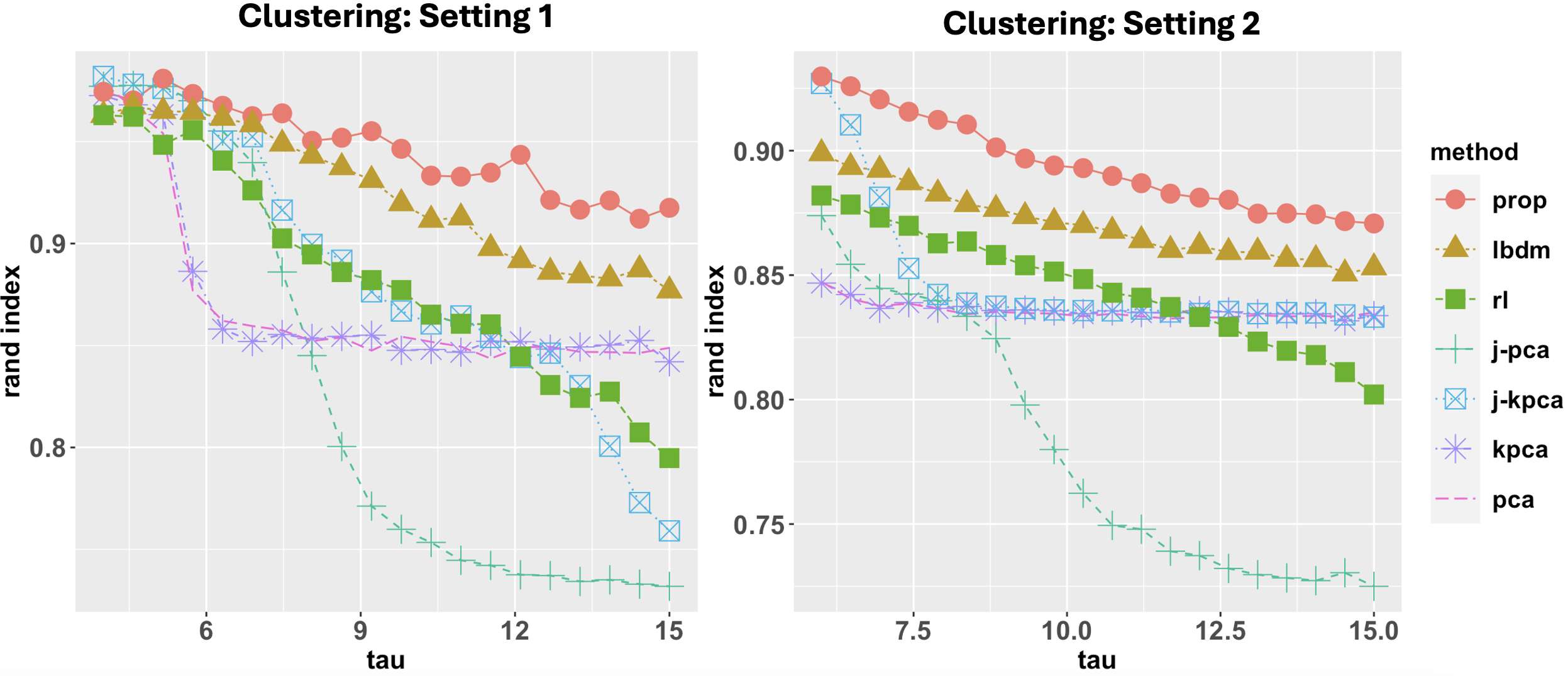
Figure 3: Comparison of simultaneous clustering performance of 7 different approaches using Rand index. The parameter $\tau$ indicates strength of added structural discrepancy between the two datasets. Left: simulation Setting 1 with identical cluster structures. Right: simulation Setting 2 with partially overlapping clusters. The proposed method does the best in leveraging the (even partially) shared cluster patterns across datasets to improve clustering of each individual dataset.

4.2 Nonlinear manifold learning

In the second study, we consider enhancing the embeddings of low-dimensional manifold structures contained in a high-dimensional noisy dataset $\{\mathbf{y}_{j}\}_{1\leq j\leq n_{2}}$, with the help of an external dataset $\{\mathbf{x}_{i}\}_{1\leq i\leq n_{1}}$ which contains stronger and cleaner signals. For the data point $\mathbf{y}_{j}$ from the nosier dataset, in terms of the model setup (1.1) and noise setup (3.20), we let $\bm{\zeta}_{j}$ be generated from multivariate Gaussian distribution with $\sigma_{2}^{2}=1.$ For the clean signal part $\mathbf{y}_{j}^{0},$ its first three coordinates are uniformly drawn from a torus in $\mathbb{R}^{3}$, i.e., for $u,v\in[0,2\pi)$, $\mathbf{y}_{j1}^{0}=\theta(2+0.8\cos u)\cos v,\mathbf{y}_{j2}^{0}=\theta(2+0.8\cos u)\sin v$ and $\mathbf{y}_{j3}^{0}=0.8\theta\sin u,$ where $\theta=0.2n^{1/2}$ characterizing the overall signal strength of the torus. For the subsequent coordinates of $\mathbf{y}_{i}^{0},$ the first 20 components (i.e., the 4-th to 23-th components) are independently drawn from a uniform distribution on $[-8,8]$, whereas the rest components are zero. The dataset $\{\mathbf{y}^{0}_{j}\}_{1\leq j\leq n_{2}}$ contains two mutually orthogonal low-dimensional signal structures. For the data point $\mathbf{x}_{i}$ from the cleaner dataset, in terms of the model setup (1.1) and noise setup (3.20), we generate $\bm{\xi}_{i}$ from multivariate Gaussian distribution with $\sigma_{1}^{2}=0.16.$ For the clean signal part $\mathbf{x}_{j}^{0},$ its first three coordinates are uniformly drawn from the same torus in $\mathbb{R}^{3}$, and the rest of the coordinates are set as zeros. As such, $\{\mathbf{x}_{i}\}_{1\leq i\leq n_{1}}$ is less noisy and only contains partially shared signal structure with $\{\mathbf{y}_{j}\}_{1\leq i\leq n_{2}}$, i.e., the torus structure.

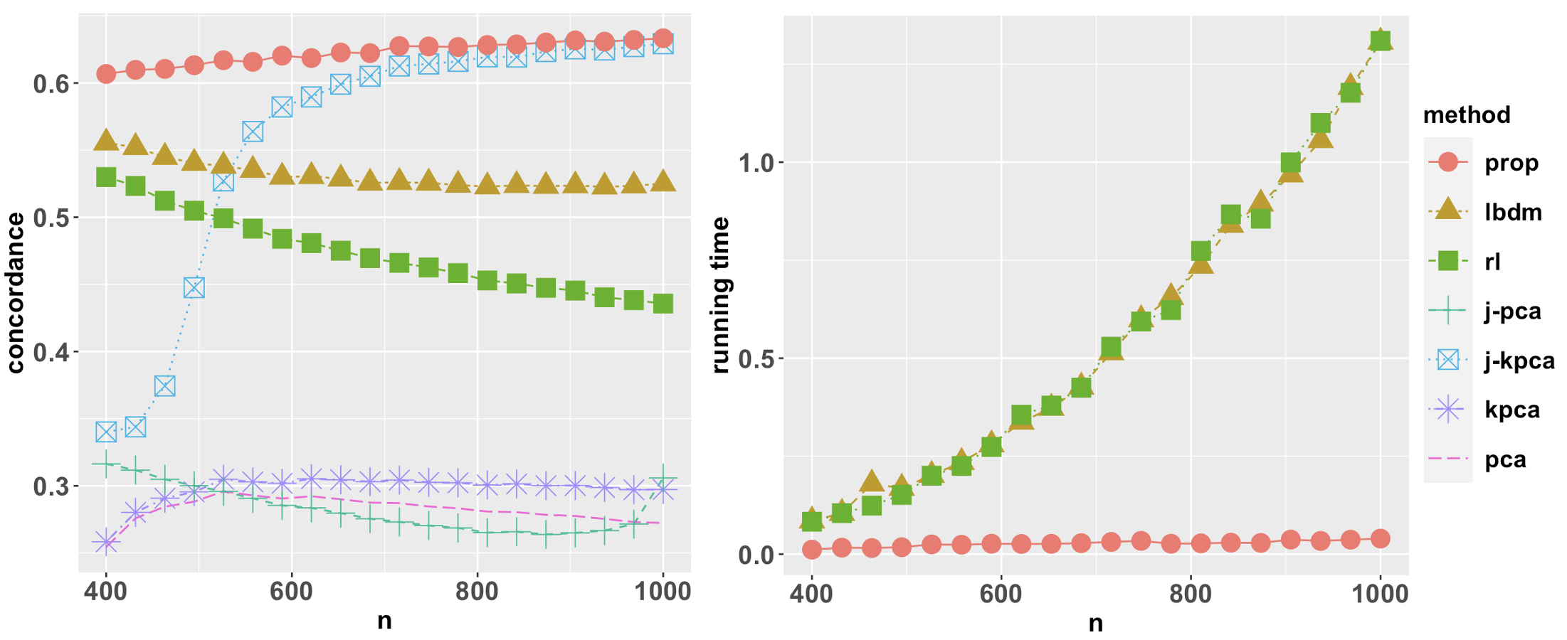
Figure 4: Comparison of nonlinear manifold learning performance of 7 different approaches. Left: concordance measures under various sample sizes. Right: running time (minutes) comparison of three related algorithms “prop”, “rl” and “lbdm,” showing the greater scalability of “prop.” The proposed algorithm has overall the best performance in retrieving the torus structures from the noisy dataset $\{\mathbf{y}_{i}\}$. Our results suggest the advantages of integrative embedding methods (e.g., “prop”) over non-integrative embedding method (“pca” and “kpca”), by leveraging the shared information from the external, cleaner dataset $\{\bm{x}_{i}\}$.

Our interest is to recover the torus structures of $\{\mathbf{y}^{0}_{j}\}$ with the help of $\{\mathbf{x}_{i}\}.$ Specifically, to evaluate the structural concordance between the obtained 3-dimensional embeddings of $\{\mathbf{y}_{i}\}_{1\leq i\leq n_{2}}$ and the original noiseless signals $\{\mathbf{y}_{i}^{0}\}_{1\leq i\leq n_{2}}$, we use Jaccard index to measure the preservation of neighborhood structures. More concretely, we consider the Jaccard index between the set of 50 nearest neighbors of the embeddings and that of the clean signals $\{\mathbf{y}_{j}^{0}\}$ and then calculate the average index value across all data points as the concordance score. In other words, for each $j\in\{1,2,...,n_{2}\}$, denote $S_{j}$ as the index set for the 50-nearest neighbors of $\mathbf{y}^{0}_{j}$ and $W_{j}$ as the index set for the 50-nearest neighbors of its low-dimensional embedding, we calculate

$$\text{concordance}:=\frac{1}{n_{2}}\sum_{j=1}^{n_{2}}\text{[Jaccard Index]}_{j},\qquad\text{[Jaccard Index]}_{j}:=\frac{|S_{j}\cap W_{j}|}{|S_{j}\cup W_{j}|}.$$ (4.3)

We examine the performance of our proposed algorithm under the setup that $p=800$ and $n_{1}=n_{2}=n,$ where $n$ range from 400 to 1000. For each $n$, we repeat the Monte Carlo simulations 1,000 times and report the averaged concordance. We compare our methods with six other methods as discussed in Section 4.1 but only assess their respective low-dimensional embeddings of the dataset $\{\mathbf{y}_{j}\}_{1\leq i\leq n_{2}}$ in term of (4.3). Among them, two embedding methods (“pca” and “kpca”) only use $\{\mathbf{y}_{j}\}_{1\leq i\leq n_{2}}$ whereas other embedding methods use both datasets.

Our results are summarized in Figure 4. Compared with alternative methods, the proposed algorithm has superior performance across all the settings in retrieving the geometric (torus) structures from the noisy dataset $\{\mathbf{y}_{i}\}_{1\leq i\leq n_{2}}$. As the sample size increases, the proposed method along with “j-kpca” and “kpca” has improved performance, whereas “rl” and “lbdm”, although achieving moderate performance under smaller sample sizes, have slightly decreased performance, possibly due to insufficient account of the high dimensionality and diverging signal strength. Comparing with non-integrative methods such as “kpca” and “pca,” our results suggest the advantages of integrative methods, such as “prop”, “j-kpca”m “lbdm” and “rl”, that borrow the shared information from the external dataset $\{\mathbf{x}_{i}\}$. Moreover, comparing with the two related kernel algorithms “rl” and “lbdm,” our proposed method is computationally more efficient, especially for handling massive datasets (Figure 4 Right).

5 Applications in integrative single-cell omics analysis

We apply the proposed method and evaluate its performance for joint analysis of single-cell omics data. By leveraging and integrating datasets with some shared biological information, we hope to improve the understanding of individual datasets, such as enhancing the underlying biological signals and capturing higher-order biological variations [7, 34]. Here we test our method by considering the important task of identifying distinct cell types based on multiple single-cell data of the same type. In Section 5.1, we analyze two single-cell RNA-seq datasets of human peripheral blood mononuclear cells (PBMCs) generated under different experimental conditions. In Section 5.2, we analyze two single-cell ATAC-seq datasets of mouse brain cells generated from different studies.

5.1 Human PBMCs single-cell RNA-seq data

The first example concerns joint analysis of two single-cell RNA-seq datasets for human PBMCs [28]. In this experiment, PBMCs were split into a stimulated group ($n_{1}=7451$ cells) and a control group ($n_{2}=6548$ cells), where the simulated group was treated with interferon beta. The distinct experimental conditions and different sequencing batches necessarily introduced structural discrepancy, or batch effects, between the two datasets, making it difficult and problematic to directly combine the two datasets. Here we are interested in identifying clusters of different cell types for each dataset, in the same spirit as our simulation studies on simultaneous biclustering. We preprocess and normalize each dataset by following the standard pipeline implemented in the Seurat R package [61], and select the $p=1,000$ most variable genes for subsequent analysis. We apply our proposed method, the Seurat spectral integration method [7, 61] (“seurat”) – arguably the most popular single-cell integration method – as well as other six methods evaluated in our simulation, to obtain clustering of both datasets.

For each method, for various choices of $\mathsf{r}$ (from 5 to 20), we first obtain $\mathsf{r}$-dimensional embeddings of both datasets, and then apply the hierarchical clustering algorithm to assign the cells into $\mathsf{r}+1$ clusters. As in Section 4.1, for each $\mathsf{r}$, the clustering results are evaluated using the Rand index (4.2), averaged across the two datasets, by comparing with the cell type annotations obtained from the original scientific publication [28, 61]. Figure 5 (Left) contains the evaluation results, where for each method, we present a boxplot of the Rand indices obtained based on different $\mathsf{r}$ values.

The proposed method achieves overall the best performance in identifying the distinct cell types. Its improvement over the methods based on separate analysis (“pca” and “kpca”) demonstrates the advantage of integrative analysis of multiple datasets. Moreover, comparing with other integrative approaches such as “j-kpca” and “seurat”, the proposed method not only achieves better clustering accuracy but shows least variability over different values of $\mathsf{r}$, demonstrating its general robustness against the choice of embedding dimensions and cluster numbers.

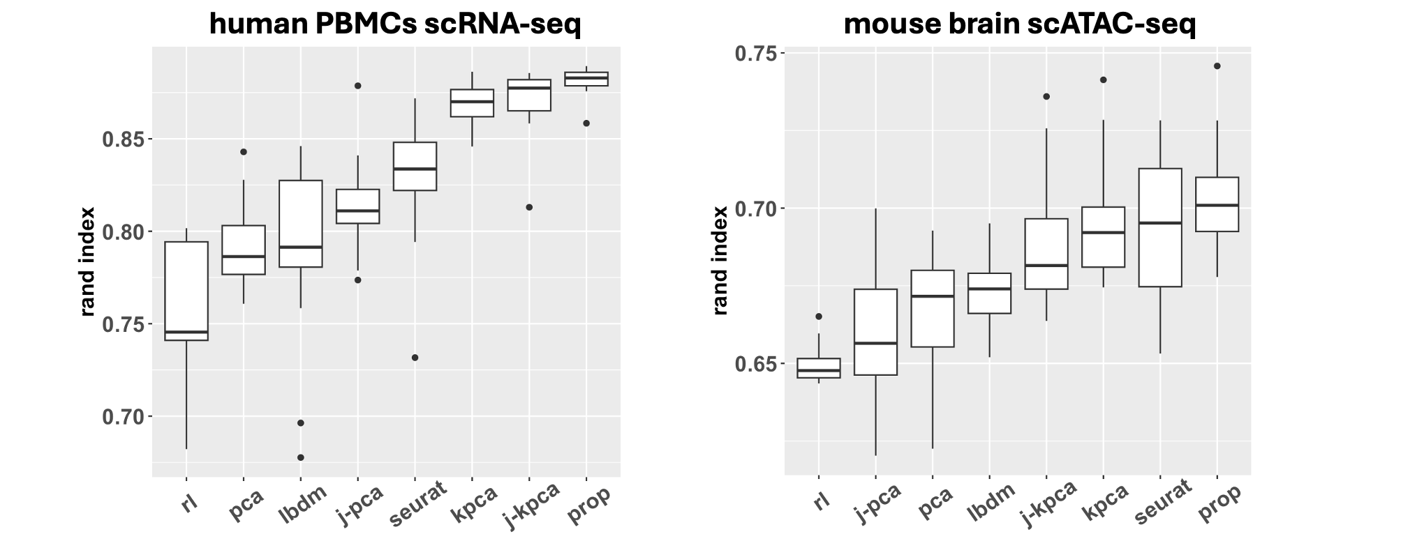
Figure 5: Comparison of eight methods for simultaneous biclustering of single-cell datasets. Each boxplot contains the Rand index for clustering accuracy obtained under various embedding dimensions ($\mathsf{r}$ from 3 to 20). Left: single-cell RNA-seq data for human peripheral blood mononuclear cells [28]. Right: single-cell ATAC-seq gene activity data for mouse brain cells. The proposed method not only achieves better clustering accuracy compared with other methods, but also shows smaller variability and therefore robustness with respect to different choices of embedding dimensions.

5.2 Mouse brain single-cell ATAC-seq data

The second example concerns integrative analysis of two single-cell ATAC-seq datasets for mouse brain cells ($n_{1}=3618$ and $n_{2}=3715$) generated from different studies [34]. ATAC-seq is a biotechnology that quantifies the genome-wide chromatin accessibility, which contains important information about epigenome dynamics and gene regulations. Each dataset contains a matrix of ATAC-seq gene activity scores, characterizing gene-specific chromatin accessibility for individual cells. Again, we preprocess and normalize the datasets following the standard pipeline in the Seurat package, and select the $p=1,000$ most variable genes for subsequent analysis. We evaluate the performance of the above eight methods in clustering the cells in both datasets under various embedding dimensions $\mathsf{r}$ (from 5 to 20), using the Rand index based on the cell type annotations provided in the original scientific publication [34]. Our results in Figure 5 (Right) again indicate the overall superior performance of the proposed method, demonstrating the benefits of integrative analysis of single-cell data, and its robustness with respect to different choices of embedding dimensions.

A Preliminary results

A.1 Background on RKHS

In this section, we summarize some results regarding the reproducing kernel Hilbert space (RKHS). Most of the results can be found in [6, 31, 51, 56, 57, 58, 59]. Consider that we observe $n$ i.i.d. samples $\{\mathbf{x}_{i}\}_{1\leq i\leq n}$ drawn from some probability distribution $\mathsf{P}$ in $\mathbb{R}^{p}$. Then the population integral operator $\mathcal{K}$ with respect to $\mathsf{P}$ and the reproducing kernel $k({\bm{x}},{\bm{y}})$, ${\bm{x}},{\bm{y}}\in\text{supp}(\mathsf{P}),$ is defined by

$${\mathcal{K}}g({\bm{x}})=\int k(\bm{x},\bm{y})g(\bm{y}){\mathsf{P}}(\mathrm{d}\bm{y}),\qquad\bm{x},\bm{y}\in\text{supp}(\mathsf{P}),$$ (A.1)

and its empirical counterpart $\mathcal{K}_{n}$ is defined by

$${\mathcal{K}_{n}}g(\bm{x})=\int k(\bm{x},\bm{y})g(\bm{y}){\mathsf{P}}_{n}(\mathrm{d}\bm{y})=\frac{1}{n}\sum_{i=1}^{n}k(\bm{x},\mathbf{x}_{i})g(\mathbf{x}_{i}),\qquad\bm{x}\in\text{supp}(\mathsf{P}),$$ (A.2)

where $\mathsf{P}_{n}$ is the empirical CDF of $\{\mathbf{x}_{i}\}.$ The RKHS $\mathcal{H}_{K}$ associated with the kernel function $k(\bm{x},\bm{y})$ in (A.1) and (A.2) is defined as the completion of the linear span of the set of functions $\{k_{\bm{x}}=k(\bm{x},\cdot):\mathbf{x}\in\text{supp}(\mathsf{P})\}$ with the inner product denoted as $\langle\cdot,\cdot\rangle_{K}$ satisfying $\langle k(\bm{x},\cdot),k(\bm{y},\cdot)\rangle_{K}=k(\bm{x},\bm{y})$ and the reproducing property $\langle k(\bm{x},\cdot),g\rangle_{K}=g(\bm{x})$ for any $g\in\mathcal{H}_{K}$. Note that $\mathcal{K}$ and $\mathcal{K}_{n}$ may be considered as self-adjoint operators on $\mathcal{H}_{K}$, or on their respective $\mathcal{L}_{2}$ spaces (that is, $\mathcal{L}_{2}(\Omega,\mathsf{P})$ and $\mathcal{L}_{2}(\Omega,\mathsf{P}_{n})$, $\Omega=\text{supp}(\mathsf{P})$).

It is easy to see that (for example, Section 2.2 of [57]) the eigenvalues of $\mathcal{K}_{n}$ coincide with $n^{-1}\mathbb{K}$, where $\mathbb{K}=(k(\mathbf{x}_{i},\mathbf{x}_{j}))_{1\leq i,j\leq n}$. The eigenfunctions $\{\widehat{\phi}_{i}\}$ associated with nonzero eigenvalues $\{\mu_{i}\}$ of $\mathcal{K}_{n}$ or $n^{-1}\mathbb{K}$ satisfy

$$\widehat{\phi}_{i}(\bm{x})=\frac{1}{\mu_{i}\sqrt{n}}\sum_{j=1}^{n}k\left(\bm{x},\mathbf{x}_{j}\right)v_{ij},\qquad\bm{x}\in\text{supp}(\mathsf{P}),$$ (A.3)

where $\mathbf{v}_{i}=(v_{i1},v_{i2},...,v_{in})^{\top}$ is the $i$-th eigenvector of $n^{-1}\mathbb{K}$, and that $\|\widehat{\phi}_{i}\|_{\mathsf{P}_{n}}=1$. The following lemma concerns the convergence of the eigenvalues and eigenfunctions of $\mathcal{K}_{n}$ to those of $\mathcal{K}$.

Lemma A.1.

For the self-adjoint operators $\mathcal{K}$ and $\mathcal{K}_{n}$ on $\mathcal{H}_{K}$, defined by (A.1) and (A.2), we have

$$\|\mathcal{K}-\mathcal{K}_{n}\|\prec\frac{1}{\sqrt{n}}.$$ (A.4)

Let $\{\gamma_{i}\}$ and $\{\phi_{i}\}$ be the eigenvalues and eigenfunctions of $\mathcal{K}$. We define the $i$-th population eigen-gap as $\mathsf{r}_{i}=\min\{\gamma_{i-1}-\gamma_{i},\gamma_{i}-\gamma_{i+1}\}$. If $n^{-1/2}=o(\mathsf{r}_{i})$, then the eigenfunctions $\{\phi_{i}^{(n)}\}$ of $\mathcal{K}_{n}$ associated with nonzero eigenvalues satisfy

$$\left\|\sqrt{\gamma_{i}}{\phi_{i}}-\sqrt{\mu_{i}}\phi_{i}^{(n)}\right\|_{K}\prec\frac{1}{\mathsf{r}_{i}\sqrt{n}},$$ (A.5)

where $\|\sqrt{\gamma_{i}}{\phi_{i}}\|_{K}=\|\sqrt{\mu_{i}}\phi_{i}^{(n)}\|_{K}=1$, and $\|\phi_{i}^{(n)}\|_{\mathsf{P}_{n}}=1$.

Proof.

This lemma is proven in [59, Proposition 1], [51, Theorem 7] and [14, Lemma 1] for the more general class of bounded and positive definite kernel functions. ∎

Lemma A.2.

Let $A$ and $\widehat{A}$ be two compact positive self-adjoint operators on a Hilbert space $H$, with nonincreasing eigenvalues $\{\lambda_{i}\}$ and $\{\widehat{\lambda}_{j}\}$ with multiplicity. Then we have $\max_{j\geq 1}|\lambda_{j}-\widehat{\lambda}_{j}|\leq\|A-\widehat{A}\|$. Let $w_{k}$ be a normalized eigenvector of $A$ associated with eigenvalue $\lambda_{k}$. If $\ell>0$ satisfies that $\min\{\lambda_{k-1}-\lambda_{k}$, $\lambda_{k}-\lambda_{k+1}\}\geq\ell$ and $\|A-\widehat{A}\|\}\leq\ell$, then $\|w_{k}-\widehat{w}_{k}\|\leq\frac{4}{\ell}\|A-\widehat{A}\|$, where $\widehat{w}_{k}$ is a normalized eigenvector of $\widehat{A}$ associated with eigenvalue $\widehat{\lambda}_{k}$.

Proof.

See Proposition 2 of [59]. ∎

Lemma A.3.

Let $S$ be a measurable space, $\nu$ be a measure on $S$ and $k$ be a measurable kernel on $S$ with RKHS $\mathcal{H}_{s}.$ Assume that $\mathcal{H}_{s}$ is compactly embedded into $\mathcal{L}_{2}(\nu,S).$ Then if $\{\Psi_{i}\}$ be the eigenfunctions of $\mathcal{H}_{s},$ then it is also an orthonormal basis for $\mathcal{L}_{2}(\nu,S).$

Proof.

See Theorem 3.1 of [60]. ∎

Lemma A.4.

For two operators $\mathcal{A}$ and $\mathcal{B},$ if they commute in the sense that $\mathcal{A}\mathcal{B}=\mathcal{B}\mathcal{A},$ then $\mathcal{A}\mathcal{B}$ and $\mathcal{B}\mathcal{A}$ have the same set of nonzero eigenvalues and eigenfunctions.

Proof.

See Section 5.1 of [43]. ∎

A.2 Some auxiliary lemmas from high-dimensional probability

We first present a few useful lemmas.

Lemma A.5.

Let $B$ be an $m\times n$ matrix, and let $\mathbf{x}$ be a mean zero, sub-Gaussian random vector in $\mathbb{R}^{n}$ with parameter bounded by $K$. Then for any $t\geq 0$, we have

$$\mathbb{P}(\|B\mathbf{x}\|_{2}\geq CK\|B\|_{F}+t)\leq\exp\bigg{(}-\frac{ct^{2}}{K^{2}\|B\|^{2}}\bigg{)}.$$

Proof.

See page 144 of [65]. ∎

The next two lemmas provide Bernstein type inequalities for bounded and sub-exponential random variables.

Lemma A.6.

Let $x_{i},1\leq i\leq n,$ be independent mean zero random variables such that $|x_{i}|\leq K$ for all $i$. Then for every $t\geq 0$

$$\mathbb{P}\left(\left|\sum_{i=1}^{n}x_{i}\right|\geq t\right)\leq 2\exp\left[-\frac{t^{2}/2}{\sum_{i=1}^{n}\mathbb{E}x_{i}^{2}+Kt/3}\right].$$

Proof.

See Theorem 2.8.4 of [65]. ∎

In the following lemmas, we will use stochastic domination to characterize the high-dimensional concentration. The next lemma collects some useful concentration inequalities for the noise vector.

Lemma A.7.

Suppose Assumption 3.9 holds. Then we have that

$$\max_{(i,j)\neq(k,l)}\frac{1}{\sigma^{2}p}\left|(\bm{\xi}_{i}-\bm{\zeta}_{j})^{\top}(\bm{\xi}_{k}-\bm{\zeta}_{l})\right|\prec{p^{-1/2}},$$

and

$$\max_{i,k}\left|\frac{1}{\sigma^{2}p}\|\bm{\xi}_{i}-\bm{\zeta}_{k}\|_{2}^{2}-1\right|\prec{p^{-1/2}}.$$

Proof.

See Lemma A.4 of [16] or Lemmas A.1 and A.2 of [15]. ∎

We also need the following proposition concerning the convergence of the empirical bandwidth $h_{n}$ defined in (2.1) and $h_{n}^{0}$ defined in (3.1). Recall (3.4).

Proposition A.8.

Suppose the assumptions of Theorem 3.12 hold and $h_{n}$ is selected according to Algorithm 1 and $h_{n}^{0}$ is defined through (3.1). Then we have $\sum_{i=1}^{r}\theta_{i}\prec h^{0}_{n}\prec\sum_{i=1}^{r}\theta_{i}$ and $|h_{n}/h_{n}^{0}-1|=\mathrm{O}_{\prec}(\eta)$.

Proof.

The proof follows the same argument as [14, Proposition 1]. ∎

B Technical proofs

B.1 Construction of auxiliary RKHSs

Note that in general $\mathcal{S}_{1}$ and $\mathcal{S}_{2}$ defined in (3.5) may not be the same. In addition, the distributions $\widetilde{\mathsf{P}}_{1}$ and $\widetilde{\mathsf{P}}_{2}$ are essentially different so that for the same kernel function $k(\cdot,\cdot),$ it may result in different Mercer’s expansions. To address this issue, we introduce two auxiliary RKHSs.

Denote

$$\mathcal{S}=\mathcal{S}_{1}\cup\mathcal{S}_{2}.$$

On $\mathcal{S},$ we define two probability measures, denoted as $\mathring{\mathtt{P}}_{1}$ and $\mathring{\mathtt{P}}_{2}$ as follows. For $\bm{w}\in\mathcal{S},$ we denote $\mathring{\mathtt{P}}_{t},t=1,2,$ that

$$\mathring{\mathtt{P}}_{t}(\bm{w})=\begin{cases}\widetilde{\mathsf{P}}_{t}(\bm{w}),&\bm{w}\in\mathcal{S}_{t}\\ 0,&\ \text{Otherwise}\end{cases}.$$ (B.1)

Based on the above two measures, we can construct RKHSs on $\mathcal{L}_{2}(\mathcal{S}).$ According to Mercer’s theorem (see Theorem 2.10 of [53]), for $(\mathcal{L}_{2}(\mathcal{S}),\mathring{\mathtt{P}}_{t}),\ t=1,2,$ we can obtain the follow decompositions for $k(\bm{w}_{1},\bm{w}_{2})$

$$k(\bm{w}_{1},\bm{w}_{2})=\sum_{j}\lambda^{a,t}_{j}\psi^{a,t}_{j}(\bm{w}_{1})\psi^{a,t}_{j}(\bm{w}_{2}),$$ (B.2)

for some positive eigenvalue sequences $\{\lambda_{j}^{a,t}\}$ and eigenfunction sequences that

$$\int_{\mathcal{S}}\psi_{j}^{a,t}(\bm{w})\psi_{i}^{a,t}(\bm{w})\mathring{\mathtt{P}}_{t}(\mathrm{d}\bm{w})=\delta_{ij}.$$

For notional simplicity, we denote these two RKHSs as $\mathring{\mathcal{H}}_{1}$ and $\mathring{\mathcal{H}}_{2}.$

B.2 Proofs of Section 3.1

Proof of Proposition 3.3.

The boundedness of the kernel follow directly from its definition and the fact that $k(\cdot,\cdot)$ is bounded.

For positive definiteness, due to similarity, we focus our discussion on the kernel $k_{1}(\bm{x}_{1},\bm{x}_{2}).$ Using the definition (3.7) and the conventions in Section B.1, we can rewrite $k_{1}(\bm{x}_{1},\bm{x}_{2})$ as

$$k_{1}(\bm{x}_{1},\bm{x}_{2})=\int_{\mathcal{S}}k(\bm{x}_{1},\bm{z})k(\bm{z},\bm{x}_{2})\mathring{\mathtt{P}}_{2}(\mathrm{d}\bm{z}).$$ (B.3)

Together with (B.2), we can write

$$k_{1}(\bm{x}_{1},\bm{x}_{2}) =\sum_{j}\sum_{i}\lambda_{j}^{a,2}\lambda_{i}^{a,2}\psi_{j}^{a,2}(\bm{x}_{1})\psi_{i}^{a,2}(\bm{x}_{2})\int_{\mathcal{S}}\psi_{j}^{a,2}(\bm{z})\psi_{i}^{a,2}(\bm{z})\mathring{\mathtt{P}}_{2}(\mathrm{d}\bm{z})$$

$$=\sum_{j}(\lambda_{j}^{a,2})^{2}\psi_{j}^{a,2}(\bm{x}_{1})\psi_{j}^{a,2}(\bm{x}_{2}).$$ (B.4)

This completes our proof for $k_{1}(\bm{x}_{1},\bm{x}_{2})$ using the reverse of Mercer’s theorem (see Exercise 2.23 of [53]).

For $k_{2}(\bm{x}_{1},\bm{x}_{2}),$ similar to the discussion of (B.2), we can show that

$$k_{2}(\bm{x}_{1},\bm{x}_{2})=\sum_{j}(\lambda_{j}^{a,1})^{2}\psi_{j}^{a,1}(\bm{x}_{1})\psi_{j}^{a,1}(\bm{x}_{2}).$$

This completes the proof for $k_{2}(\bm{x}_{1},\bm{x}_{2}).$ ∎

B.3 Proofs of Section 3.2

Proof of Propositions 3.6.

According to (B.3) and (B.2), we can also write that

$$k_{1}(\bm{x}_{1},\bm{x}_{2})=\sum_{j}\sum_{i}\lambda_{j}^{a,2}\lambda_{i}^{a,1}\psi_{j}^{a,2}(\bm{x}_{1})\psi_{i}^{a,1}(\bm{x}_{2})\int_{\mathcal{S}}\psi_{j}^{a,2}(\bm{z})\psi_{i}^{a,1}(\bm{z})\mathring{\mathtt{P}}_{2}(\mathrm{d}\bm{z}).$$ (B.5)

Similarly, we can also write

$$k_{2}(\bm{y}_{1},\bm{y}_{2})=\sum_{j}\sum_{i}\lambda_{j}^{a,2}\lambda_{i}^{a,1}\psi_{j}^{a,2}(\bm{y}_{1})\psi_{i}^{a,1}(\bm{y}_{2})\int_{\mathcal{S}}\psi_{j}^{a,2}(\bm{z})\psi_{i}^{a,1}(\bm{z})\mathring{\mathtt{P}}_{1}(\mathrm{d}\bm{z}).$$

Let $\ell_{2}(\mathbb{R}):=\{\bm{a}=(a_{i})_{i\in\mathbb{N}}\in\mathbb{R}^{\infty}|a_{i}\in\mathbb{R}\ \text{and}\ \sum_{i=1}^{\infty}a_{i}^{2}<\infty\}.$ We denote two operators $\mathcal{T}_{1}$ and $\mathcal{T}_{2}$ on $\ell_{2}(\mathbb{R})$ as follows

$$\mathcal{T}_{1}\bm{a}=\left(\lambda_{j}^{a,2}\sum_{i=1}^{\infty}a_{i}\int_{\mathcal{S}}\psi_{j}^{a,2}(\bm{z})\psi_{i}^{a,1}(\bm{z})\mathring{\mathtt{P}}_{2}(\mathrm{d}\bm{z})\right)_{j\in\mathbb{N}},$$

and

$$\mathcal{T}_{2}\bm{a}=\left(\lambda_{j}^{a,1}\sum_{i=1}^{\infty}a_{i}\int_{\mathcal{S}}\psi_{j}^{a,1}(\bm{z})\psi_{i}^{a,2}(\bm{z})\mathring{\mathtt{P}}_{1}(\mathrm{d}\bm{z})\right)_{j\in\mathbb{N}}.$$

It is straightforward to see that $\mathcal{T}_{1}$ and $\mathcal{T}_{2}$ commutes on $\ell_{2}(\mathbb{R}).$ Therefore, according to Lemma A.4, $\mathcal{T}_{1}\mathcal{T}_{2}$ and $\mathcal{T}_{2}\mathcal{T}_{1}$ have the same nonzero eigenvalues. To conclude our proof, we will show that the nonzero eigenvalues of $\mathcal{K}_{1}$ coincide with those of $\mathcal{T}_{1}\mathcal{T}_{2},$ and those of $\mathcal{K}_{2}$ coincide with those of $\mathcal{T}_{2}\mathcal{T}_{1}.$

Under the assumption that $\mathcal{H}_{1}$ and $\mathcal{H}_{2}$ are compactly embedded into some common space $\mathcal{N},$ we can use the conventions in Section B.1 to conclude that these exist some common measurable space $\mathring{\mathcal{N}}$ so that $\mathring{\mathcal{H}}_{1}$ and $\mathring{\mathcal{H}}_{2}$ are compactly embedded into $\mathcal{L}_{2}(\mathring{\mathcal{N}},\mathring{\mathsf{P}}_{1})$ and $\mathcal{L}_{2}(\mathring{\mathcal{N}},\mathring{\mathsf{P}}_{2}),$ respectively. Suppose $\phi(\cdot)$ is an eigenfunction of $\mathcal{K}_{1}$ associated with some nonzero eigenvalue $\lambda$. That is,

$$\mathcal{K}_{1}\phi(\bm{x})=\lambda\phi(\bm{x}),\ \bm{x}\in\mathcal{S}_{1}.$$ (B.6)

By Lemma A.3 and the conventions of Section B.1, we can expand $\phi(\bm{x})$ on the common space $\mathring{\mathcal{N}}$ via $\mathcal{L}_{2}(\mathring{\mathcal{N}},\mathring{\mathsf{P}}_{2})$ using the basis of $\mathring{\mathcal{H}}_{2}.$ Consequently, we can write that for some constants $b_{i}\equiv b_{i}(\phi),\ i\in\mathbb{N}$ and $(b_{i})\in\ell_{2}(\mathbb{R})$ so that

$$\phi(\bm{x})=\sum_{i=1}^{\infty}b_{i}\psi^{a,2}_{i}(\bm{x}).$$

Together with (B.5) and Definition 3.4 as well as the conventions in Section B.1, we have that

$$\mathcal{K}_{1}\phi(\bm{x}) =\int_{\mathcal{S}}k_{1}(\bm{x},\bm{y})\sum_{i=1}^{\infty}b_{i}\psi^{a,2}_{i}(\bm{y})\mathring{\mathtt{P}}_{1}(\mathrm{d}\bm{y})$$

$$=\int_{\mathcal{S}}\sum_{j}\sum_{i}\lambda_{j}^{a,2}\lambda_{i}^{a,1}\psi_{j}^{a,2}(\bm{x})\psi_{i}^{a,1}(\bm{y})\int_{\mathcal{S}}\psi_{j}^{a,2}(\bm{z})\psi_{i}^{a,1}(\bm{z})\mathring{\mathtt{P}}_{2}(\mathrm{d}\bm{z})\sum_{t=1}^{\infty}b_{t}\psi_{t}^{a,2}(\bm{y})\mathring{\mathtt{P}}_{1}(\mathrm{d}\bm{y})$$

$$=\sum_{j=1}^{\infty}\alpha_{j}\psi_{j}^{a,2}(\bm{x}),$$

where $\alpha_{j}$ is denoted as

$$\alpha_{j}:=\lambda_{j}^{a,2}\sum_{i}\int_{\mathcal{S}}\psi_{j}^{a,2}(\bm{z})\psi_{i}^{a,1}(\bm{z})\mathring{\mathtt{P}}_{2}(\mathrm{d}\bm{z})\lambda_{i}^{a,1}\sum_{t=1}^{\infty}b_{t}\int_{\mathcal{S}}\psi_{i}^{a,1}(\bm{y})\psi_{t}^{a,2}(\bm{y})\mathring{\mathtt{P}}_{1}(\mathrm{d}\bm{y}).$$

Since the discussion holds for all $\bm{x},$ together with (B.6), we conclude that

$$\alpha_{j}=\lambda b_{j},\ j\in\mathbb{N}$$ (B.7)

Denote $\bm{b}=(b_{j})_{j\in\mathbb{N}}$ and $\bm{\alpha}=(\alpha_{j})_{j\in\mathbb{N}}.$ Using the definitions of $\mathcal{T}_{1}$ and $\mathcal{T}_{2},$ we can rewrite (B.7) as follows

$$\mathcal{T}_{1}\mathcal{T}_{2}\bm{b}=\lambda\bm{b}.$$

This shows that $\lambda$ is also an eigenvalues of $\mathcal{T}_{1}\mathcal{T}_{2}$ and conclude the proof that the nonzero eigenvalues of $\mathcal{K}_{1}$ coincide with those of $\mathcal{T}_{1}\mathcal{T}_{2}.$ Similarly, we can show that the eigenvalues of $\mathcal{K}_{2}$ coincide with those of $\mathcal{T}_{2}\mathcal{T}_{1}.$ This completes our proof.

∎

Proof of Theorem 3.8.

We start with the convergence of the eigenvalues (3.14). Since $\mathbb{N}_{01}$ and $\mathbb{N}_{02}$ in (3.11) have the same nonzero eigenvalues, we focus our discussion on $\mathbb{N}_{01}.$ For $\mathbb{N}_{01}=(N_{ij}^{01}),$ we see that

$$N^{01}_{ij}=\frac{1}{n_{1}n_{2}}\sum_{k=1}^{n_{2}}k(\mathbf{x}^{0}_{i},\mathbf{y}^{0}_{k})k(\mathbf{x}^{0}_{j},\mathbf{y}^{0}_{k}).$$

Using the conventions in Section B.2, we now introduce the following auxiliary matrix that $\mathbb{W}_{01}=(W_{ij}^{01})\in\mathbb{R}^{n_{1}\times n_{1}},$ where

$$W_{ij}^{01}=\frac{1}{n_{1}}\int_{\mathcal{S}}k(\mathbf{x}^{0}_{i},\bm{y})k(\bm{y},\mathbf{x}^{0}_{j})\mathring{\mathtt{P}}_{2}(\mathrm{d}\bm{y})\equiv\frac{1}{n_{1}}k_{1}(\mathbf{x}_{i}^{0},\mathbf{x}_{j}^{0}).$$ (B.8)

Denote the eigenvalues of $\mathbb{W}_{01}$ as $\{\lambda_{i}^{01}\}.$ Then according to Proposition 3.3 and Lemma A.1, we have that

$$\sup_{i}|\lambda_{i}^{01}-\gamma_{i}|\prec\frac{1}{\sqrt{n_{1}}}.$$ (B.9)

Moreover, for each $1\leq i\neq j\leq n_{1}$, conditional on $\mathbf{x}_{i}^{0}$ and $\mathbf{x}_{j}^{0}$, $N_{ij}^{01}$ is essentially a sum of independent bounded random variables $k(\mathbf{x}^{0}_{i},\mathbf{y}^{0}_{k})k(\mathbf{x}^{0}_{j},\mathbf{y}^{0}_{k}),k=1,2,...,n_{2}$, satisfying

$$\mathbb{E}\left[k(\mathbf{x}^{0}_{i},\mathbf{y}^{0}_{k})k(\mathbf{y}^{0}_{k},\mathbf{x}^{0}_{j})|\mathbf{x}^{0}_{i},\mathbf{x}^{0}_{j}\right]=n_{1}W_{ij}^{01}.$$

Therefore, for each pair of $i,j,$ we can apply Lemma A.6 to obtain that

$$\left|\frac{1}{n_{2}}\sum_{k=1}^{n_{2}}k(\mathbf{x}^{0}_{i},\mathbf{y}^{0}_{k})k(\mathbf{y}^{0}_{k},\mathbf{x}^{0}_{j})-n_{1}W_{ij}^{01}\right|\prec n_{2}^{-1/2}.$$ (B.10)

Equivalently, we have that

$$n_{1}N_{ij}^{01}=n_{1}W_{ij}^{01}+\mathrm{O}_{\prec}\left(n_{2}^{-1/2}\right).$$

By Gershgorin circle theorem, we readily have that

$$\|\mathbb{N}_{01}-\mathbb{W}_{01}\|\prec\frac{1}{\sqrt{n}_{2}}.$$ (B.11)

Combining (B.9) and (B.11), we can conclude the proof of (3.16).

Then we proceed to the proof of the eigenfunctions. Due to similarity, we focus on the proof of (3.18). For the matrix $\mathbb{W}_{01}$ defined according to (B.8), we denote its eigenvectors associated with the eigenvalues $\{\lambda_{i}^{01}\}$ as $\{\mathbb{u}_{i}^{01}\}.$ Then for $\bm{x}\in\mathcal{S}_{1},$ we denote that

$$\phi^{01}_{i}(\bm{x})=\frac{1}{\lambda^{01}_{i}\sqrt{n_{1}}}\sum_{j=1}^{n_{1}}{k}_{1}(\bm{x},\mathbf{x}^{0}_{j})u^{01}_{ij}$$

where $\mathbf{u}^{01}_{i}=(u^{01}_{i1},\cdots,u^{01}_{in_{1}})^{\top}.$ According to (B.9) and Lemma A.1, we find that

$$\left\|\sqrt{\lambda_{i}^{01}}\phi_{i}^{01}(\bm{x})-\sqrt{\gamma_{i}}\phi_{i}(\bm{x})\right\|_{K_{1}}\prec\frac{1}{\mathsf{r}_{i}\sqrt{n}_{1}},$$

where $\|\cdot\|_{K_{1}}$ is the induced norm of the RKHS built on $\mathcal{L}_{2}(\mathcal{S}_{1},\widetilde{\mathsf{P}}_{1})$ (or equivalently, on $\mathcal{L}_{2}(\mathcal{S},\mathring{\mathtt{P}}_{1})$ using the convention of Section B.3) using the kernel $k_{1}.$ Moreover, using the property of the reproducing kernel (see equation (2.31) of [53]), we have that

$$\left|\sqrt{\lambda_{i}^{01}}\phi_{i}^{01}(\bm{x})-\sqrt{\gamma_{i}}\phi_{i}(\bm{x})\right|\leq\sqrt{k_{1}(\bm{x},\bm{x})}\left\|\sqrt{\lambda_{i}^{01}}\phi_{i}^{01}(\bm{x})-\sqrt{\gamma_{i}}\phi_{i}(\bm{x})\right\|_{K_{1}}\prec\frac{1}{\mathsf{r}_{i}\sqrt{n}_{1}},$$ (B.12)

where we used the boundedness of the kernel $k_{1}$ in Proposition 3.3.

Moreover, we have that

$$\quad\left|\sqrt{\lambda_{i}^{01}}\phi_{i}^{01}(\bm{x})-\sqrt{\lambda_{i}}\widehat{\phi}^{0}_{i}(\bm{x})\right|$$

$$=\frac{1}{\sqrt{n_{1}}}\bigg{|}\frac{1}{\sqrt{\lambda^{01}_{i}}}\sum_{j=1}^{n_{1}}{k}_{1}(\bm{x},\mathbf{x}^{0}_{j})u^{01}_{ij}-\frac{1}{\sqrt{\lambda_{i}}}\sum_{j=1}^{n_{1}}\widehat{k}^{0}_{1}(\bm{x},\mathbf{x}^{0}_{j})u^{0}_{ij}\bigg{|}$$

$$\leq\frac{1}{\sqrt{n_{1}}}\left|\frac{1}{\sqrt{\lambda^{01}_{i}}}\sum_{j=1}^{n_{1}}\widehat{k}^{0}_{1}(\bm{x},\mathbf{x}^{0}_{j})u^{0}_{ij}-\frac{1}{\sqrt{\lambda_{i}}}\sum_{j=1}^{n_{1}}\widehat{k}^{0}_{1}(\bm{x},\mathbf{x}^{0}_{j})u^{0}_{ij}\right|+\frac{1}{\sqrt{n_{1}}}\left|\frac{1}{\sqrt{\lambda^{01}_{i}}}\sum_{j=1}^{n_{1}}{k}_{1}(\bm{x},\mathbf{x}^{0}_{j})u^{0}_{ij}-\frac{1}{\sqrt{\lambda^{01}_{i}}}\sum_{j=1}^{n_{1}}\widehat{k}^{0}_{1}(\bm{x},\mathbf{x}^{0}_{j})u^{0}_{ij}\right|$$

$$\quad+\frac{1}{\sqrt{n_{1}}}\bigg{|}\frac{1}{\sqrt{\lambda^{01}_{i}}}\sum_{j=1}^{n_{1}}{k}_{1}(\bm{x},\mathbf{x}^{0}_{j})u^{01}_{ij}-\frac{1}{\sqrt{\lambda^{01}_{i}}}\sum_{j=1}^{n_{1}}{k}_{1}(\bm{x},\mathbf{x}^{0}_{j})u^{0}_{ij}\bigg{|}$$

$$:=E_{1}+E_{2}+E_{3}.$$ (B.13)

For $E_{1},$ by Cauchy–Schwarz inequality, we have that

$$E_{1}\leq\frac{1}{\sqrt{n_{1}}}\frac{|\lambda_{i}-\lambda^{01}_{i}|}{\sqrt{\lambda_{i}\lambda^{01}_{i}}}\sqrt{\sum_{j=1}^{n_{1}}(k_{1}(\bm{x},\mathbf{x}_{j}^{0}))^{2}}\|\mathbb{u}^{0}_{i}\|_{2}.$$ (B.14)

Together with the assumption that $1\leq i\leq\mathsf{K}$ (c.f. (3.14)), (3.16) and (B.11), we have that

$$E_{1}\prec\frac{1}{\sqrt{n_{2}}},$$

where we used the boundnedness of the kernel $k_{1}$ in Proposition 3.3. For $E_{2},$ we have that

$$E_{2} =\frac{1}{\sqrt{\lambda^{01}_{i}}\sqrt{n_{1}}}\bigg{|}\sum_{j=1}^{n_{1}}[{k}_{1}(\bm{x},\mathbf{x}^{0}_{j})-\widehat{k}^{0}_{1}(\bm{x},\mathbf{x}^{0}_{j})]u^{0}_{ij}\bigg{|}$$ (B.15)

$$\leq\frac{1}{\sqrt{\lambda_{i}^{01}}}\sqrt{\frac{1}{n_{1}}\sum_{j=1}^{n_{1}}\left[k_{1}(\bm{x},\mathbf{x}_{j}^{0})-\widehat{k}_{1}(\bm{x},\mathbf{x}_{j}^{0})\right]^{2}}$$

$$\leq\frac{1}{\sqrt{\lambda^{01}_{i}}}\max_{1\leq j\leq n_{1}}\bigg{|}\frac{1}{n_{2}}\sum_{k=1}^{n_{2}}k(\bm{x},\mathbf{y}^{0}_{k})k(\mathbf{y}^{0}_{k},\mathbf{x}^{0}_{j})-\int_{\mathcal{S}}k(\bm{x},\bm{z})k(\bm{z},\mathbf{x}^{0}_{j})\mathring{\mathtt{P}}_{2}(\mathrm{d}\bm{z})\bigg{|}$$

$$\prec n_{2}^{-1/2},$$

where in the second step we used Cauchy-Schwarz inequality, in the third step we used the fact that both $k_{1}$ and $\widehat{k}_{1}$ are bounded and the definition in (3.12), and in the last step we used a discussion similar to (B.10) with Lemma A.6. Similarly, for $E_{3}$, by Cauchy-Schwarz inequality, we have

$$E_{3} =\frac{1}{\sqrt{\lambda^{01}_{i}}\sqrt{n_{1}}}\bigg{|}\sum_{j=1}^{n_{1}}{k}_{1}(\bm{x},\mathbf{x}^{0}_{j})(u^{01}_{ij}-u^{0}_{ij})\bigg{|}\prec\|\mathbb{u}^{01}_{i}-\mathbb{u}^{0}_{i}\|_{2}.$$ (B.16)

Consequently, it suffices to control $\|\mathbb{u}^{01}_{i}-\mathbb{u}^{0}_{i}\|_{2}.$ According to the assumption of (3.17), (3.16) and (B.11), we see that with high probability, for some constant $c>0$

$$\lambda_{i}-\lambda_{i+1}\geq c\mathsf{r}_{i},\qquad\lambda_{i-1}-\lambda_{i}\geq c\mathsf{r}_{i},\qquad\|\mathbb{N}_{01}-\mathbb{W}_{01}\|\leq c\mathsf{r}_{i}/2.$$

Then we can use Lemma A.2 and (B.11) to show that

$$\|\bar{\mathbb{u}}_{i}-\mathbb{u}^{0}_{i}\|_{2}\prec\frac{1}{\mathsf{r}_{i}\sqrt{n_{2}}}.$$

Consequently, we have that $E_{3}\prec\mathsf{r}_{i}^{-1}n_{2}^{-1/2}.$ Inserting all the above controls into (B.3), we see that

$$\left|\sqrt{\lambda_{i}^{01}}\phi_{i}^{01}(\bm{x})-\sqrt{\lambda_{i}}\widehat{\phi}^{0}_{i}(\bm{x})\right|\prec\frac{1}{\mathsf{r}_{i}\sqrt{n_{2}}}+\frac{1}{\sqrt{n_{2}}}.$$

Together with (B.12), we can complete the proof of (3.18).

∎

B.4 Proof of Section 3.3

Proof of Theorem 3.12.

For $\mathbb{N}_{1}=(N^{1}_{ij})_{1\leq i,j\leq n}$ defined in (3.22), we have that

$$N^{1}_{ij}=\frac{1}{n_{1}n_{2}}\sum_{k=1}^{n_{2}}f\bigg{(}\frac{\|\mathbf{x}_{i}-\mathbf{y}_{k}\|_{2}}{h^{1/2}_{n}}\bigg{)}f\bigg{(}\frac{\|\mathbf{y}_{k}-\mathbf{x}_{j}\|_{2}}{h^{1/2}_{n}}\bigg{)},$$

where we used the short-hand notation that $f(x)=\exp(-x^{2}).$ During the proof, we will also use the following auxiliary quantity

$$\widetilde{N}^{1}_{ij}=\frac{1}{n_{1}n_{2}}\sum_{k=1}^{n_{2}}f\bigg{(}\frac{\|\mathbf{x}_{i}-\mathbf{y}_{k}\|_{2}}{\sqrt{h_{n}^{0}}}\bigg{)}f\bigg{(}\frac{\|\mathbf{y}_{k}-\mathbf{x}_{j}\|_{2}}{\sqrt{h_{n}^{0}}}\bigg{)}.$$

where $h_{n}^{0}$ is the clean bandwidth as defined in (3.1). Moreover, for $\mathbb{N}_{01}=(N_{ij}^{01})$ defined in (3.11), we have that

$$N^{01}_{ij}=\frac{1}{n_{1}n_{2}}\sum_{k=1}^{n_{2}}f\bigg{(}\frac{\|\mathbf{x}^{0}_{i}-\mathbf{y}^{0}_{k}\|_{2}}{\sqrt{h_{n}^{0}}}\bigg{)}f\bigg{(}\frac{\|\mathbf{y}^{0}_{k}-\mathbf{x}^{0}_{j}\|_{2}}{\sqrt{h_{n}^{0}}}\bigg{)}.$$

We start with the proof of the eigenvalue convergence (3.24) and control $\|\mathbb{N}_{01}-\mathbb{N}_{1}\|$. We will control the entry-wise difference by studying

$$|N^{1}_{ij}-N^{01}_{ij}| \leq|N^{1}_{ij}-\widetilde{N}^{1}_{ij}|+|\widetilde{N}^{1}_{ij}-N^{01}_{ij}|.$$

First, under the model assumption (1.1), we have that

$$|\widetilde{N}^{1}_{ij}-N^{01}_{ij}|$$

$$=\bigg{|}\frac{1}{n_{1}n_{2}}\sum_{k=1}^{n_{2}}\exp\bigg{(}-\frac{\|\mathbf{x}_{i}-\mathbf{y}_{k}\|^{2}_{2}+\|\mathbf{y}_{k}-\mathbf{x}_{j}\|_{2}^{2}}{h_{n}}\bigg{)}-\frac{1}{n_{1}n_{2}}\sum_{k=1}^{n_{2}}\exp\bigg{(}-\frac{\|\mathbf{x}^{0}_{i}-\mathbf{y}^{0}_{k}\|_{2}^{2}+\|\mathbf{y}^{0}_{k}-\mathbf{x}^{0}_{j}\|_{2}^{2}}{h_{n}}\bigg{)}\bigg{|}$$

$$=\bigg{|}\frac{1}{n_{1}n_{2}}\sum_{k=1}^{n_{2}}\exp\bigg{(}-\frac{\|\mathbf{x}^{0}_{i}-\mathbf{y}^{0}_{k}\|^{2}_{2}+\|\mathbf{y}^{0}_{k}-\mathbf{x}^{0}_{j}\|_{2}^{2}}{h_{n}}\bigg{)}\nu(k,i,j)\bigg{|},$$ (B.17)

where $\nu(k,i,j)$ is defined as

$$\nu(k,i,j):=\exp\bigg{(}-\frac{\|{\bm{\xi}}_{i}-\bm{\zeta}_{k}\|_{2}^{2}+\|\bm{\zeta}_{k}-{\bm{\xi}}_{j}\|_{2}^{2}-2({\bm{\xi}}_{i}-\bm{\zeta}_{k})^{\top}(\mathbf{x}_{i}^{0}-\mathbf{y}_{k}^{0})-2({\bm{\zeta}}_{k}-\bm{\xi}_{j})^{\top}(\mathbf{y}_{k}^{0}-\mathbf{x}_{j}^{0})}{h_{n}}\bigg{)}-1.$$

By Lemma A.7, we have

$$\max_{i,k}\|\bm{\xi}_{i}-\bm{\zeta}_{k}\|_{2}^{2}\prec\sigma^{2}p.$$

Moreover, by Lemma A.5 and the setup in (3.4), we have that

$$\max_{i\neq j}\|\mathbf{x}_{i}^{0}-\mathbf{y}_{k}^{0}\|_{2}^{2}\prec\sum_{i=1}^{r}\theta_{i},\ \max_{i,k}|({\bm{\xi}}_{i}-\bm{\zeta}_{k})^{\top}(\mathbf{x}_{i}^{0}-\mathbf{y}_{k}^{0})|\prec\sigma(\sum_{i=1}^{r}\theta_{i})^{1/2}.$$ (B.18)

According to Proposition A.8, we see that

$$\nu(k,i,j)\prec\frac{\sigma^{2}p+\sigma(\sum_{i=1}^{r}\theta_{i})^{1/2}}{\sum_{i=1}^{r}\theta_{i}}.$$

Inserting the above bounds into (B.4), we readily see that

$$|\widetilde{N}^{1}_{ij}-N^{01}_{ij}|\prec\frac{\sigma^{2}p+\sigma(\sum_{i=1}^{r}\theta_{i})^{1/2}}{n_{1}\sum_{i=1}^{r}\theta_{i}}.$$ (B.19)

Second, similar to the above discussions, we have that

$$|N^{1}_{ij}-\widetilde{N}^{1}_{ij}| =\left|\frac{1}{n_{1}n_{2}}\sum_{k=1}^{n_{2}}\exp\bigg{(}-\frac{\|\mathbf{x}_{i}-\mathbf{y}_{k}\|^{2}_{2}+\|\mathbf{y}_{k}-\mathbf{x}_{j}\|_{2}^{2}}{h_{n}}\bigg{)}-\frac{1}{n_{1}n_{2}}\sum_{k=1}^{n_{2}}\exp\bigg{(}-\frac{\|\mathbf{x}_{i}-\mathbf{y}_{k}\|^{2}_{2}+\|\mathbf{y}_{k}-\mathbf{x}_{j}\|_{2}^{2}}{h_{n}^{0}}\bigg{)}\right|$$

$$=\frac{1}{n_{1}n_{2}}\left|\sum_{k=1}^{n_{2}}\exp\bigg{(}-\frac{\|\mathbf{x}_{i}-\mathbf{y}_{k}\|^{2}_{2}+\|\mathbf{y}_{k}-\mathbf{x}_{j}\|_{2}^{2}}{h_{n}}\upsilon(k,i,j)\right|,$$ (B.20)

where $\upsilon(k,i,j)$ is defined as

$$\upsilon(k,i,j):=1-\exp\bigg{(}\frac{\|\mathbf{x}_{i}-\mathbf{y}_{k}\|^{2}_{2}+\|\mathbf{y}_{k}-\mathbf{x}_{j}\|_{2}^{2}}{h_{n}}-\frac{\|\mathbf{x}_{i}-\mathbf{y}_{k}\|^{2}_{2}+\|\mathbf{y}_{k}-\mathbf{x}_{j}\|_{2}^{2}}{h_{n}^{0}}\bigg{)}.$$

Using (B.18) and Proposition A.8, we find that

$$\upsilon(k,i,j)\prec\eta.$$

This implies that

$$|N_{ij}^{1}-\widetilde{N}_{ij}^{1}|\prec\frac{\eta}{n_{1}}.$$

Together with (B.19), we have that

$$|N_{ij}^{1}-N_{ij}^{01}|\prec\frac{\eta}{n_{1}}.$$

By Gershgorin circle theorem, we can conclude that

$$\|\mathbb{N}_{1}-\mathbb{N}_{01}\|\prec\eta.$$ (B.21)

This completes the proof of (3.24).

For the eigenvectors convergence (3.26), due to similarity, we only prove the results for $\left\langle\mathbf{u}_{i},\mathbf{u}_{i}^{0}\right\rangle.$ Recall that for any positive definite matrix $\mathbb{A}$ admitting the spectral decomposition $\mathbb{A}=\sum_{i=1}^{n}\lambda_{i}(\mathbb{A})\bm{\beta}_{i}\bm{\beta}_{i}^{\top}$, it holds that

$$\bm{\beta}_{i}\bm{\beta}_{i}^{\top}=\frac{1}{2\pi\mathrm{i}}\oint_{\Gamma}(z{\bf I}-\mathbb{A})^{-1}\mathrm{d}z,$$

where $\Gamma\equiv\Gamma_{i}\subset\mathbb{C}$ is some simply connected contour only containing $\lambda_{i}(\mathbb{A})$ but no other eigenvalues of $\mathbb{A}$. The above integral representation serves as the starting point of our analysis.

Now we denote the contour $\Gamma_{i}:=\mathsf{B}(\gamma_{i},\frac{\mathsf{\mathsf{r}_{i}}}{C}),$ for some large constant $C>0,$ where $\mathsf{B}(\gamma_{i},\frac{\mathsf{r}_{i}}{C})$ is the disk centered at $\gamma_{i}$ with radius $\frac{\mathsf{r}_{i}}{C}$ with $\mathsf{r}_{i}$ is defined in (3.15). Combining (3.24), (3.16) and the assumption of (3.25), we find that for $1\leq i\leq\mathsf{K}$

$$|\mu_{i}-\gamma_{i}|\leq|\mu_{i}-\lambda_{i}|+|\lambda_{i}-\gamma_{i}|\prec\eta+n_{1}^{-1/2}+n_{2}^{-1/2}=\mathsf{o}(\mathsf{r}_{i}),$$

and for $1\leq j\neq i\leq\mathsf{K},$ we have that for some constant $C>0,$ with high-probability

$$|\mu_{j}-\gamma_{i}|\geq\left||\mu_{j}-\gamma_{j}|-|\gamma_{j}-\gamma_{i}|\right|\geq C\mathsf{r}_{i}.$$

This shows that with high probability, $\mu_{i}$ is the only eigenvalue inside $\Gamma_{i}.$ Consequently, it yields that

$$\mathbb{u}_{i}\mathbb{u}_{i}^{\top}=\frac{1}{2\pi\mathrm{i}}\oint_{\Gamma_{i}}(z{\bf I}-\mathbb{N}_{1})^{-1}\mathrm{d}z.$$

This further implies that, with high probability

$$\langle\mathbb{u}_{i},\mathbb{u}_{i}^{0}\rangle^{2} =\frac{1}{2\pi\mathrm{i}}\oint_{\Gamma_{i}}(\mathbb{u}_{i}^{0})^{\top}(z{\bf I}-\mathbb{N}_{1})^{-1}\mathbb{u}_{i}^{0}\mathrm{d}z$$ (B.22)

$$=\frac{1}{2\pi\mathrm{i}}\oint_{\Gamma_{i}}(\mathbb{u}_{i}^{0})^{\top}(z{\bf I}-\mathbb{N}_{01})^{-1}\mathbb{u}_{i}^{0}\mathrm{d}z+\frac{1}{2\pi\mathrm{i}}\oint_{\Gamma_{i}}(\mathbb{u}_{i}^{0})^{\top}[(z{\bf I}-\mathbb{N}_{1})^{-1}-(z{\bf I}-\mathbb{N}_{01})^{-1}]\mathbb{u}_{i}^{0}\mathrm{d}z$$

$$:={\sf L}_{1}+{\mathsf{L}_{2}},$$ (B.23)

For the first term $\mathsf{L}_{1},$ by residual theorem, with high probability, we have that

$$\mathsf{L}_{1}=1.$$

For the second term $\mathsf{L}_{2},$ we have that

$$|\mathsf{L}_{2}|\leq\frac{2\pi\mathsf{r}_{i}}{2\pi}\sup_{z\in\Gamma_{i}}\left\|(z{\bf I}-\mathbb{N}_{1})^{-1}-(z{\bf I}-\mathbb{N}_{01})^{-1}\right\|.$$ (B.24)

To control the right-hand side of (B.24), according to the resolvent identity, we have that

$$(z{\bf I}-\mathbb{N}_{1})^{-1}-(z{\bf I}-\mathbb{N}_{01})^{-1}=(z{\bf I}-\mathbb{N}_{1})^{-1}[\mathbb{N}_{1}-\mathbb{N}_{01}](z{\bf I}-\mathbb{N}_{01})^{-1}.$$ (B.25)

Recall that $\{\lambda_{i}\}$ are the eigenvalues of $\mathbb{N}_{01}.$ According to (3.15), (3.16), the assumption of (3.25) as well as the definition of $\Gamma_{i}$, we have that

$$\inf_{z\in\Gamma_{i}}\min\{|\lambda_{i}-z|,|\lambda_{i-1}-z|,|\lambda_{i+1}-z|\}\asymp\mathsf{r}_{i}.$$

This yields that

$$\sup_{z\in\Gamma_{i}}\left\|(z{\bf I}-\mathbb{N}_{01})^{-1}\right\|\prec\frac{1}{\mathsf{r}_{i}}.$$

With a similar discussion and (3.24), we can also prove that This yields that

$$\sup_{z\in\Gamma_{i}}\left\|(z{\bf I}-\mathbb{N}_{1})^{-1}\right\|\prec\frac{1}{\mathsf{r}_{i}}.$$

Combining the above controls with (B.21) and (B.25), together with (B.24), we readily see that

$$\mathsf{L}_{2}\prec\frac{\eta}{\mathsf{r}_{i}}.$$

Inserting the above results into (B.23), we can therefore conclude the proof.

∎

Proof of Corollary 3.13.

For the eigenvalues, (3.29) follows directly from (3.24) and (3.16). For the eigenfunctions, due to similarity, we focus on (3.30). Recall (3.13). We decompose that

$$|\sqrt{\gamma_{i}}{\phi}_{i}(\bm{x})-\sqrt{\mu_{i}}\widehat{\phi}_{i}(\bm{x})|\leq|\sqrt{\gamma_{i}}{\phi}_{i}(\bm{x})-\sqrt{\lambda_{i}}\widehat{\phi}^{0}_{i}(\bm{x})|+|\sqrt{\lambda_{i}}\widehat{\phi}^{0}_{i}(\bm{x})-\sqrt{\mu_{i}}\widehat{\phi}_{i}(\bm{x})|.$$ (B.26)

Note that the first term on the RHS of the above equation can be controlled by (3.18). It suffices to control the second term using a discussion similar to (B.3). By definition, we have that

$$\quad|\sqrt{\lambda_{i}}\widehat{\phi}^{0}_{i}(\bm{x})-\sqrt{\mu}\widehat{\phi}_{i}(\bm{x})|$$

$$=\frac{1}{\sqrt{n_{1}}}\bigg{|}\frac{1}{\sqrt{\lambda_{i}}}\sum_{j=1}^{n_{1}}\widehat{k}^{0}_{1}(\bm{x},\mathbf{x}^{0}_{j})u^{0}_{ij}-\frac{1}{\sqrt{\mu_{i}}}\sum_{j=1}^{n_{1}}\widehat{k}_{1}(\bm{x},\mathbf{x}_{j})u_{ij}\bigg{|}$$

$$\leq\frac{1}{\sqrt{n_{1}}}\bigg{|}\frac{1}{\sqrt{\lambda_{i}}}\sum_{j=1}^{n_{1}}\widehat{k}^{0}_{1}(\bm{x},\mathbf{x}^{0}_{j})u^{0}_{ij}-\frac{1}{\sqrt{\mu_{i}}}\sum_{j=1}^{n_{1}}\widehat{k}^{0}_{1}(\bm{x},\mathbf{x}^{0}_{j})u^{0}_{ij}\bigg{|}+\frac{1}{\sqrt{n_{1}}}\bigg{|}\frac{1}{\sqrt{\mu_{i}}}\sum_{j=1}^{n_{1}}\widehat{k}^{0}_{1}(\bm{x},\mathbf{x}^{0}_{j})u^{0}_{ij}-\frac{1}{\sqrt{\mu_{i}}}\sum_{j=1}^{n_{1}}\widehat{k}_{1}(\bm{x},\mathbf{x}_{j})u^{0}_{ij}\bigg{|}$$

$$\quad+\frac{1}{\sqrt{n_{1}}}\bigg{|}\frac{1}{\sqrt{\mu_{i}}}\sum_{j=1}^{n_{1}}\widehat{k}_{1}(\bm{x},\mathbf{x}_{j})u^{0}_{ij}-\frac{1}{\sqrt{\mu_{i}}}\sum_{j=1}^{n_{1}}\widehat{k}_{1}(\bm{x},\mathbf{x}^{0}_{j})u_{ij}\bigg{|}$$

$$:=F_{1}+F_{2}+F_{3}.$$ (B.27)

For $F_{1},$ by a discussion similar to (B.14), we have that

$$F_{1}\prec|\lambda_{i}-\mu_{i}|\prec\eta,$$

where in the second step we used (3.24). For $F_{2},$ by a discussion similar to (B.15), we have that

$$F_{2}\prec\max_{1\leq j\leq n_{1},1\leq k\leq n_{2}}w(k,j),$$

where $w(k,j)$ follows that

$$w(k,j) :=\left|\exp\bigg{(}-\frac{\|\bm{x}-\mathbf{y}^{0}_{k}\|^{2}_{2}}{h_{n}^{0}}\bigg{)}\exp\bigg{(}-\frac{\|\mathbf{y}^{0}_{k}-\mathbf{x}^{0}_{j}\|_{2}^{2}}{h_{n}^{0}}\bigg{)}-\exp\bigg{(}-\frac{\|\bm{x}-\mathbf{y}_{k}\|^{2}_{2}}{h_{n}}\bigg{)}\exp\bigg{(}-\frac{\|\mathbf{y}_{k}-\mathbf{x}_{j}\|_{2}^{2}}{h_{n}}\bigg{)}\right|$$

$$\leq\left|\exp\bigg{(}-\frac{\|\bm{x}-\mathbf{y}^{0}_{k}\|^{2}_{2}}{h_{n}^{0}}\bigg{)}\exp\bigg{(}-\frac{\|\mathbf{y}^{0}_{k}-\mathbf{x}^{0}_{j}\|_{2}^{2}}{h_{n}^{0}}\bigg{)}-\exp\bigg{(}-\frac{\|\bm{x}-\mathbf{y}_{k}\|^{2}_{2}}{h^{0}_{n}}\bigg{)}\exp\bigg{(}-\frac{\|\mathbf{y}_{k}-\mathbf{x}_{j}\|_{2}^{2}}{h_{n}^{0}}\bigg{)}\right|$$

$$+\left|\exp\bigg{(}-\frac{\|\bm{x}-\mathbf{y}_{k}\|^{2}_{2}}{h^{0}_{n}}\bigg{)}\exp\bigg{(}-\frac{\|\mathbf{y}_{k}-\mathbf{x}_{j}\|_{2}^{2}}{h_{n}^{0}}\bigg{)}-\exp\bigg{(}-\frac{\|\bm{x}-\mathbf{y}_{k}\|^{2}_{2}}{h_{n}}\bigg{)}\exp\bigg{(}-\frac{\|\mathbf{y}_{k}-\mathbf{x}_{j}\|_{2}^{2}}{h_{n}}\bigg{)}\right|$$

$$:=F_{21}+F_{22}.$$

For $F_{21},$ by a discussion similar to (B.4), we find that

$$F_{21}\prec\eta.$$

For $F_{22},$ by a discussion similar to (B.20), we find that

$$F_{22}\prec\eta.$$

Consequently, we find that

$$F_{2}\prec\eta.$$

For $F_{3},$ by a discussion similar to (B.16), we have that

$$F_{3}\prec\|\mathbb{u}_{i}-\mathbb{u}^{0}_{i}\|_{2}=\sqrt{2(1-\mathbb{u}_{i}^{\top}\mathbb{u}_{i}^{0})}\asymp\sqrt{|1-(\mathbb{u}_{i}^{\top}\mathbb{u}_{i}^{0})^{2}|}\prec\sqrt{\frac{\eta}{\mathsf{r}_{i}}},$$

where in the last step we used (3.26).

Inserting the above bounds into (B.4), in light of (B.26), together with (3.18), we can conclude the proof of (3.30).

∎

C Automated hyperparameter selection

As demonstrated in our theoretical analysis in Section 3, under our specified assumptions, any constant value of $\omega$ within the range of 0 to 1 ensures the attainment of high-quality embeddings. In practice, to optimize the empirical performance and improve automation of the method, we recommend using a resampling approach following Section E of [14].

An algorithm based on resampling was introduced for determining the percentile parameter, as outlined in Algorithm 1 of [16], which has also been utilized in [13, 18]. The method offers the flexibility to select $\mathsf{s}$ through a resampling technique, aimed at distinguishing the larger outlier eigenvalues from the bulk eigenvalues within the kernel matrix $\mathbb{K}$. Here, the outlier eigenvalues represent the signal components, while the bulk eigenvalues correspond to the noise components. A fundamental insight guiding this strategy is the proximity of bulk eigenvalues to each other, resulting in ratios of consecutive eigenvalues close to one (refer to Remark 2.9 of [16] for elaboration). With $\mathsf{s}$ chosen, the algorithm is succinctly outlined below for completeness.

Algorithm C.1 (Algorithm in Section E.1 of [14]).

We follow the steps below to choose the percentile $\omega.$

1. For a pre-selected sequence of percentiles$\{\omega\}_{i=1}^{T},$ calculated the associated bandwidths according to (2.1), denoted as $\{h_{i}\}_{i=1}^{T}.$

2. For each $1\leq i\leq T,$ calculate the eigenvalues of $\mathbb{K}_{n,i}$, constructed using the bandwidth $h_{i}.$ Denote the eigenvalues of $\mathbb{K}_{n,i}$ in the decreasing order as $\{\lambda_{k}^{(i)}\}_{k=1}^{n}.$

3. For some $\mathsf{s}>0,$ denote

   $$\mathsf{k}(\omega_{i}):=\max_{1\leq k\leq n-1}\left\{k\bigg{|}\frac{\lambda_{k}^{(i)}}{\lambda_{k+1}^{(i)}}\geq 1+\mathsf{s}\right\}.$$

   Choose the percentile $\omega$ such that

   $$\omega=\max_{i}[\mathop{\rm arg\max}_{\omega_{i}}\mathsf{k}(\omega_{i})].$$ (C.1)

Specifically, the final step can be substituted with alternative criteria based on users’ objectives. Here, we opt for selecting the largest criterion to enhance robustness.

References

- [1] G. Andrew, R. Arora, J. Bilmes, and K. Livescu. Deep canonical correlation analysis. In International conference on machine learning, pages 1247–1255, 2013.
- [2] R. Argelaguet, D. Arnol, D. Bredikhin, Y. Deloro, B. Velten, J. C. Marioni, and O. Stegle. Mofa+: a statistical framework for comprehensive integration of multi-modal single-cell data. Genome biology, 21:1–17, 2020.
- [3] R. Argelaguet, A. S. Cuomo, O. Stegle, and J. C. Marioni. Computational principles and challenges in single-cell data integration. Nature biotechnology, 39(10):1202–1215, 2021.
- [4] A. Baysoy, Z. Bai, R. Satija, and R. Fan. The technological landscape and applications of single-cell multi-omics. Nature Reviews Molecular Cell Biology, 24(10):695–713, 2023.
- [5] K. M. Boehm, P. Khosravi, R. Vanguri, J. Gao, and S. P. Shah. Harnessing multimodal data integration to advance precision oncology. Nature Reviews Cancer, 22(2):114–126, 2022.
- [6] M. L. Braun. Accurate error bounds for the eigenvalues of the kernel matrix. Journal of Machine Learning Research, 7(82):2303–2328, 2006.
- [7] A. Butler, P. Hoffman, P. Smibert, E. Papalexi, and R. Satija. Integrating single-cell transcriptomic data across different conditions, technologies, and species. Nature biotechnology, 36(5):411–420, 2018.
- [8] K. Cao, Y. Hong, and L. Wan. Manifold alignment for heterogeneous single-cell multi-omics data integration using pamona. Bioinformatics, 38(1):211–219, 2022.
- [9] T. Chari and L. Pachter. The specious art of single-cell genomics. PLOS Computational Biology, 19(8):e1011288, 2023.
- [10] M.-Y. Cheng and H.-T. Wu. Local linear regression on manifolds and its geometric interpretation. Journal of the American Statistical Association, 108(504):1421–1434, 2013.
- [11] U. Dayal, M. Castellanos, A. Simitsis, and K. Wilkinson. Data integration flows for business intelligence. In Proceedings of the 12th International Conference on Extending Database Technology: Advances in Database Technology, pages 1–11, 2009.
- [12] X. Ding. High dimensional deformed rectangular matrices with applications in matrix denoising. Bernoulli, 26(1):387 – 417, 2020.
- [13] X. Ding. Spiked sample covariance matrices with possibly multiple bulk components. Random Matrices: Theory and Applications, 10(01):2150014, 2021.
- [14] X. Ding and R. Ma. Learning low-dimensional nonlinear structures from high-dimensional noisy data: an integral operator approach. The Annals of Statistics, 51(4):1744–1769, 2023.
- [15] X. Ding and H.-T. Wu. On the spectral property of kernel-based sensor fusion algorithms of high dimensional data. IEEE Transactions on Information Theory, 67(1):640–670, 2021.
- [16] X. Ding and H.-T. Wu. Impact of signal-to-noise ratio and bandwidth on graph Laplacian spectrum from high-dimensional noisy point cloud. IEEE Transactions on Information Theory, 69(3):1899–1931, 2023.
- [17] X. Ding and H.-T. Wu. How do kernel-based sensor fusion algorithms behave under high dimensional noise? Information and Inference: A journal of the IMA (in press), 2024.
- [18] X. Ding and F. Yang. Spiked separable covariance matrices and principal components. The Annals of Statistics, 49(2):1113–1138, 2021.
- [19] N. El Karoui and H. Wu. Graph connection Laplacian methods can be made robust to noise. The Annals of Statistics, 44(1):346–372, 2016.
- [20] L. Erdős and H. Yau. A Dynamical Approach to Random Matrix Theory. Courant Lecture Notes. Courant Institute of Mathematical Sciences, New York University, 2017.
- [21] F. Gustafsson. Statistical Sensor Fusion. Studentlitteratur, 2010.
- [22] L. Haghverdi, A. T. Lun, M. D. Morgan, and J. C. Marioni. Batch effects in single-cell RNA-sequencing data are corrected by matching mutual nearest neighbors. Nature biotechnology, 36(5):421–427, 2018.
- [23] D. R. Hardoon, S. Szedmak, and J. Shawe-Taylor. Canonical correlation analysis: An overview with application to learning methods. Neural computation, 16(12):2639–2664, 2004.
- [24] H. Hotelling. Relations between two sets of variates. Biometrika, 28(3/4):321–377, 1936.
- [25] B. Hou, S. Sanjari, N. Dahlin, S. Bose, and U. Vaidya. Sparse learning of dynamical systems in RKHS: an operator-theoretic approach. In International Conference on Machine Learning, pages 13325–13352, 2023.
- [26] P. Hünermund and E. Bareinboim. Causal inference and data fusion in econometrics. The Econometrics Journal, page utad008, 2023.
- [27] A. R. Joyce and B. Ø. Palsson. The model organism as a system: integrating ’omics’ data sets. Nature reviews Molecular cell biology, 7(3):198–210, 2006.
- [28] H. M. Kang, M. Subramaniam, S. Targ, M. Nguyen, L. Maliskova, E. McCarthy, E. Wan, S. Wong, L. Byrnes, C. M. Lanata, et al. Multiplexed droplet single-cell RNA-sequencing using natural genetic variation. Nature biotechnology, 36(1):89–94, 2018.
- [29] M. Kang, E. Ko, and T. B. Mersha. A roadmap for multi-omics data integration using deep learning. Briefings in Bioinformatics, 23(1):bbab454, 2022.
- [30] A. Kline, H. Wang, Y. Li, S. Dennis, M. Hutch, Z. Xu, F. Wang, F. Cheng, and Y. Luo. Multimodal machine learning in precision health: A scoping review. npj Digital Medicine, 5(1):171, 2022.
- [31] V. Koltchinskii and E. Giné. Random matrix approximation of spectra of integral operators. Bernoulli, 6(1):113 – 167, 2000.
- [32] P. L. Lai and C. Fyfe. Kernel and nonlinear canonical correlation analysis. International journal of neural systems, 10(05):365–377, 2000.
- [33] Y. Li, P. Nair, X. H. Lu, Z. Wen, Y. Wang, A. A. K. Dehaghi, Y. Miao, W. Liu, T. Ordog, J. M. Biernacka, et al. Inferring multimodal latent topics from electronic health records. Nature communications, 11(1):2536, 2020.
- [34] M. D. Luecken, M. Büttner, K. Chaichoompu, A. Danese, M. Interlandi, M. F. Müller, D. C. Strobl, L. Zappia, M. Dugas, M. Colomé-Tatché, et al. Benchmarking atlas-level data integration in single-cell genomics. Nature methods, 19(1):41–50, 2022.
- [35] R. Ma, E. D. Sun, D. Donoho, and J. Zou. Principled and interpretable alignability testing and integration of single-cell data. Proceedings of the National Academy of Sciences, 121(10):e2313719121, 2024.
- [36] A. Maan and J. Smith. Characterizing information imbalance in biomedical datasets. Journal of Computational Biology, 20(3):123–138, 2024.
- [37] H. Maan, L. Zhang, C. Yu, M. J. Geuenich, K. R. Campbell, and B. Wang. Characterizing the impacts of dataset imbalance on single-cell data integration. Nature Biotechnology, pages 1–10, 2024.
- [38] N. F. Marshall and M. J. Hirn. Time coupled diffusion maps. Applied and Computational Harmonic Analysis, 45(3):709–728, 2018.
- [39] M. Martínez-García and E. Hernández-Lemus. Data integration challenges for machine learning in precision medicine. Frontiers in medicine, 8:784455, 2022.
- [40] M. Mazumder, C. Banbury, X. Yao, B. Karlaš, W. Gaviria Rojas, S. Diamos, G. Diamos, L. He, A. Parrish, H. R. Kirk, et al. Dataperf: Benchmarks for data-centric AI development. Advances in Neural Information Processing Systems, 36, 2024.
- [41] M. Meister and I. Steinwart. Optimal learning rates for localized svms. Journal of Machine Learning Research, 17(194):1–44, 2016.
- [42] T. Michaeli, W. Wang, and K. Livescu. Nonparametric canonical correlation analysis. In International conference on machine learning, pages 1967–1976, 2016.
- [43] D. A. Miller. Quantum mechanics for scientists and engineers. Cambridge University Press, 2008.
- [44] K. R. Moon, D. van Dijk, Z. Wang, S. Gigante, D. B. Burkhardt, W. S. Chen, K. Yim, A. van den Elzen, M. J. Hirn, R. R. Coifman, et al. Visualizing structure and transitions in high-dimensional biological data. Nature Biotechnology, 37(12):1482–1492, 2019.
- [45] J. A. Omiye, H. Gui, S. J. Rezaei, J. Zou, and R. Daneshjou. Large language models in medicine: The potentials and pitfalls: A narrative review. Annals of Internal Medicine, 177(2):210–220, 2024.
- [46] R. Petegrosso, Z. Li, and R. Kuang. Machine learning and statistical methods for clustering single-cell RNA-sequencing data. Briefings in bioinformatics, 21(4):1209–1223, 2020.
- [47] K. Pham and G. Chen. Large-scale spectral clustering using diffusion coordinates on landmark-based bipartite graphs. In Proceedings of the Twelfth Workshop on Graph-Based Methods for Natural Language Processing (TextGraphs-12), pages 28–37, 2018.
- [48] W. M. Rand. Objective criteria for the evaluation of clustering methods. Journal of the American Statistical Association, 66(336):846–850, 1971.
- [49] N. Rappoport and R. Shamir. Multi-omic and multi-view clustering algorithms: review and cancer benchmark. Nucleic acids research, 46(20):10546–10562, 2018.
- [50] F. Reverter, E. Vegas, and J. M. Oller. Kernel-PCA data integration with enhanced interpretability. BMC systems biology, 8:1–9, 2014.
- [51] L. Rosasco, M. Belkin, and E. D. Vito. On learning with integral operators. Journal of Machine Learning Research, 11(30):905–934, 2010.
- [52] N. Sapoval, A. Aghazadeh, M. G. Nute, D. A. Antunes, A. Balaji, R. Baraniuk, C. Barberan, R. Dannenfelser, C. Dun, M. Edrisi, et al. Current progress and open challenges for applying deep learning across the biosciences. Nature Communications, 13(1):1728, 2022.
- [53] B. Schölkopf and A. Smola. Learning with Kernels: Support Vector Machines, Regularization, Optimization, and Beyond. Adaptive computation and machine learning. MIT Press, 2002.
- [54] C. Shen, Y.-T. Lin, and H.-T. Wu. Robust and scalable manifold learning via landmark diffusion for long-term medical signal processing. The Journal of Machine Learning Research, 23(1):3742–3771, 2022.
- [55] C. Shen and H.-T. Wu. Scalability and robustness of spectral embedding: landmark diffusion is all you need. Information and Inference: A Journal of the IMA, 11(4):1527–1595, 2022.
- [56] T. Shi, M. Belkin, and B. Yu. Data spectroscopy: Learning mixture models using eigenspaces of convolution operators. In Proceedings of the 25th International Conference on Machine Learning, ICML ’08, page 936–943, 2008.
- [57] T. Shi, M. Belkin, and B. Yu. Data spectroscopy: Eigenspaces of convolution operators and clustering. The Annals of Statistics, 37(6B):3960 – 3984, 2009.
- [58] S. Smale and D.-X. Zhou. Learning theory estimates via integral operators and their approximations. Constructive Approximation, 26:153–172, 2007.
- [59] S. Smale and D.-X. Zhou. Geometry on probability spaces. Constructive Approximation, 30(3):311–323, 2009.
- [60] I. Steinwart and C. Scovel. Mercer’s theorem on general domains: On the interaction between measures, kernels, and RKHSs. Constructive Approximation, 35:363–417, 2012.
- [61] T. Stuart, A. Butler, P. Hoffman, C. Hafemeister, E. Papalexi, W. M. Mauck, Y. Hao, M. Stoeckius, P. Smibert, and R. Satija. Comprehensive integration of single-cell data. Cell, 177(7):1888–1902, 2019.
- [62] T. Stuart and R. Satija. Integrative single-cell analysis. Nature reviews genetics, 20(5):257–272, 2019.
- [63] I. Subramanian, S. Verma, S. Kumar, A. Jere, and K. Anamika. Multi-omics data integration, interpretation, and its application. Bioinformatics and biology insights, 14:1177932219899051, 2020.
- [64] R. Talmon and H.-T. Wu. Latent common manifold learning with alternating diffusion: analysis and applications. Applied and Computational Harmonic Analysis, 47(3):848–892, 2019.
- [65] R. Vershynin. High-dimensional probability: An introduction with applications in data science, volume 47. Cambridge university press, 2018.
- [66] H.-T. Wu. Design a metric robust to complicated high dimensional noise for efficient manifold denoising. arXiv preprint arXiv:2401.03921, 2024.
- [67] H.-T. Wu and N. Wu. Think globally, fit locally under the Manifold Setup: Asymptotic Analysis of Locally Linear Embedding. Annals of Statistics, 46(6B):3805–3837, 2018.
- [68] L. Xiong, K. Tian, Y. Li, W. Ning, X. Gao, and Q. C. Zhang. Online single-cell data integration through projecting heterogeneous datasets into a common cell-embedding space. Nature Communications, 13(1):6118, 2022.
- [69] S.-Y. Yeh, H.-T. Wu, R. Talmon, and M.-P. Tsui. Landmark Alternating Diffusion. arXiv preprint: 2404.19649, 2024.
- [70] L. Yu, X. Wang, Q. Mu, S. S. T. Tam, D. S. C. Loi, A. K. Chan, W. S. Poon, H.-K. Ng, D. T. Chan, J. Wang, et al. scone-seq: A single-cell multi-omics method enables simultaneous dissection of phenotype and genotype heterogeneity from frozen tumors. Science Advances, 9(1):eabp8901, 2023.
- [71] J. Zhao, X. Xie, X. Xu, and S. Sun. Multi-view learning overview: Recent progress and new challenges. Information Fusion, 38:43–54, 2017.