Trace Moments for Schrödinger Operators with Matrix White Noise and the Rigidity of the Multivariate Stochastic Airy Operator

Abstract.

We study the semigroups of random Schrödinger operators of the form $\widehat{H}f=-\frac{1}{2}f^{\prime\prime}+(V+\xi)f$, where $f:I\to\mathbb{F}^{r}$ ($\mathbb{F}=\mathbb{R},\mathbb{C},\mathbb{H}$) are vector-valued functions on a possibly infinite interval $I\subset\mathbb{R}$ that satisfy a mix of Robin and Dirichlet boundary conditions, $V$ is a deterministic diagonal potential with power-law growth at infinity, and $\xi$ is a matrix white noise. Our main result consists of Feynman-Kac formulas for trace moments of the form $\mathbf{E}\Big{[}\prod_{k=1}^{n}\mathrm{Tr}\big{[}\mathrm{e}^{-t_{k}\widehat{H}}\big{]}\Big{]}$ ($n\in\mathbb{N}$, $t_{k}>0$).

One notable example covered by our main result consists of the multivariate stochastic Airy operator (SAO) of Bloemendal and Virág [5], which characterizes the soft-edge eigenvalue fluctuations of critical rank-$r$ spiked Wishart and GO/U/SE random matrices. As a corollary of our main result, we prove that if $V$’s growth is at least linear (this includes the multivariate SAO), then $\widehat{H}$’s spectrum is number rigid in the sense of Ghosh and Peres [32]. Together with the rigidity of the scalar SAO [6, 27], this completes the characterization of number rigidity in the soft-edge limits of Gaussian $\beta$-ensembles and their finite-rank spiked versions.

1. Introduction

1.1. General Setup and Main Result

In this paper, we are interested in the semigroup theory of a class of random vector-valued Scrhödinger operators defined as follows: Let $\mathbb{F}$ be the field of real numbers $\mathbb{R}$, the field of complex numbers $\mathbb{C}$, or the ring of quaternions $\mathbb{H}$. Let $r>0$ be a fixed integer, and $I\subset\mathbb{R}$ be a (possibly infinite) interval. Consider the operator

$$Hf(i,x)=-\tfrac{1}{2}f^{\prime\prime}(i,x)+V(i,x)f(i,x),\qquad f:I\to\mathbb{F}^{r},$$

where $\big{(}f(i,\cdot)\big{)}_{1\leq i\leq r}$ denote the components of a vector-valued function $f$, the second derivative $f^{\prime\prime}$ acts on the variable $x\in I$ only, and $V(i,\cdot)$ are locally integrable deterministic functions with sufficient growth when $I$ is infinite (see Assumption 2.8). Assume that $H$ acts on functions whose components $f(i,\cdot)$ satisfy a mix of Robin boundary conditions $f^{\prime}(i,c)+\alpha f(i,c)=0$ ($\alpha\in\mathbb{R}$) and Dirichlet boundary conditions $f(i,c)=0$ at the boundary points $c\in\partial I$; if there are any (see Assumption 2.4).

We are interested in random perturbations of $H$ of the form

(1.1) $$\widehat{H}=H+\xi,$$

where $\xi$ is a matrix white noise. That is, if we let $\cdot^{*}$ denote conjugation in $\mathbb{F}$, then $\xi$ is the singular matrix multiplication operator

$$\xi f(i,\cdot)=\sum_{j=1}^{n}\xi_{i,j}f(j,\cdot),$$

where $\xi_{i,j}=\xi_{j,i}^{*}$ for all $1\leq i,j\leq r$, and informally, we view $(\xi_{i,i})_{1\leq i\leq r}$ as the derivatives of i.i.d. Brownian motions in $\mathbb{R}$ and $(\xi_{i,j})_{1\leq i<j\leq r}$ as the derivatives of i.i.d. Brownian motions in $\mathbb{F}$ (see Definition 2.7 for more details).

The aim of this paper is to provide a new avenue to study the eigenvalues of $\widehat{H}$ via probabilistic representations of the semigroup $\mathrm{e}^{-t\widehat{H}}$. Our main result in this direction, Theorem 4.8, consists of Feynman-Kac formulas for the joint moments

(1.2) $$\mathbf{E}\left[\mathrm{Tr}\big{[}\mathrm{e}^{-t_{1}\widehat{H}}\big{]}\mathrm{Tr}\big{[}\mathrm{e}^{-t_{2}\widehat{H}}\big{]}\cdots\mathrm{Tr}\big{[}\mathrm{e}^{-t_{n}\widehat{H}}\big{]}\right],\qquad n\in\mathbb{N},~{}t_{1},\ldots,t_{n}\geq 0.$$

Letting $\lambda_{1}(\widehat{H})\leq\lambda_{2}(\widehat{H})\leq\cdots$ denote the eigenvalues of $\widehat{H}$, we recall that

$$\textstyle\mathrm{Tr}\big{[}\mathrm{e}^{-t\widehat{H}}\big{]}=\sum_{k=1}^{\infty}\mathrm{e}^{-t\lambda_{k}(\widehat{H})}\qquad\text{for every }t>0.$$

Thus, a calculation of the quantities (1.2) provides a means of characterizing the distribution of $\widehat{H}$’s eigenvalue point process via its Laplace transform’s joint moments.

A notable feature of our Feynman-Kac formulas when $r>1$ is the following insight: In addition to the usual Brownian motion $\big{(}B(t)\big{)}_{t\geq 0}$ (coming from the diffusion operator $f\mapsto-\tfrac{1}{2}f^{\prime\prime}$), the dynamics are decorated by a continuous-time random walk $\big{(}U(t)\big{)}_{t\geq 0}$ on the complete graph with $r$ vertices, whose jumps times $\tau_{1}\leq\tau_{2}\leq\cdots$ are conditioned to coincide with self-intersections of both $U$ and $B$. That is, there must exists a way to partition the jump times into pairs $\{\tau_{\ell_{1}},\tau_{\ell_{2}}\}$ such that

1. the jumps in $U$ that occur at times $\tau_{\ell_{1}}$ and $\tau_{\ell_{2}}$ are between the same two vertices in $\{1,\ldots,r\}$, and

2. $B(\tau_{\ell_{1}})=B(\tau_{\ell_{2}})$.

Among other things, this induces a surprisingly rich combinatorial structure in the mixed moments (1.2), coming from counting paths of the random walk $U$ for which such pairings exist. We refer to the statement of Theorem 4.8 for the full details, and to Section 1.3.3 for a high-level explanation of this result and how it is proved.

The remainder of this introduction is organized as follows: In Section 1.2, we discuss the motivation for our work (mainly, understanding the multivariate stochastic Airy operators), as well as an application in the study of number rigidity of eigenvalue point processes. In Section 1.3, we provide a high-level explanation of our method of proof, and we survey past results related to the main technical innovation in this paper. In Section 1.4, we formulate an open problem regarding a pathwise Feynman-Kac formula for $\widehat{H}$. Then, in Section 1.5, we discuss the organization of the rest of the paper. Finally, Section 1.6 contains some acknowledgements.

1.2. Motivation and Application

1.2.1. Motivation 1: Multivariate Stochastic Airy Operators

Our main motivation for developing the semigroup theory of $\widehat{H}$ comes from the special case where $I=(0,\infty)$, $V(i,x)=\frac{rx}{2}$, and $\frac{1}{\sqrt{2}}\xi$ is a standard matrix white noise (that is, the derivative of a matrix Brownian motion with GOE/GUE/GSE increments; see Remark 2.10 for more details). In this special case, $2\widehat{H}$ is the multivariate stochastic Airy operator (SAO) introduced by Bloemendal and Virág in [5] (see also [4, 50] for previous results concerning the scalar case $r=1$).

The interest in the multivariate SAO lies in the fact that its spectrum describes the asymptotic soft-edge scaling limits of critical rank-$r$ perturbations of Wishart and Gaussian invariant ensembles; the so-called spiked models. More specifically, consider an $r\times r$ generalized matrix of the form

(1.3) $$W=\sum_{i=1}^{r}(-\overline{\alpha}_{i})u_{i}u_{i}^{\dagger},\qquad\overline{\alpha}_{i}\in(-\infty,\infty],$$

where the vectors $u_{i}\in\mathbb{F}^{r}$ form an orthonormal basis and $\dagger$ denotes the conjugate transpose, and let $2\widehat{H}$ be the multivariate SAO with boundary conditions

(1.4) $$\begin{cases}f^{\prime}(i,0)+\overline{\alpha}_{i}f(i,0)=0&\text{if }\overline{\alpha}_{i}\in\mathbb{R},\\ f(i,0)=0&\text{if }\overline{\alpha}_{i}=-\infty.\end{cases}$$

1. On the one hand, [5, Theorem 1.2] showed that $2\widehat{H}$’s spectrum describes the limiting fluctuations (as $n\to\infty$) of the top eigenvalues of $n\times n$ random matrices of the form $X_{n}+(W_{n}\oplus 0_{n-r})$, where $X_{n}$ is a GOE, GUE, or GSE matrix (depending on whether $\beta=1,2,$ or $4$),

   (1.5) $$W_{n}\approx\sqrt{n}\,\mathrm{Id}_{r}-n^{1/6}W$$

   is a critical additive perturbation of rank $r$, and $0_{k}$ and $\mathrm{Id}_{k}$ denote respectively the $k\times k$ zero and identity matrices.

2. On the other hand, [5, Theorem 1.3] showed that $2\widehat{H}$’s spectrum also describes the limit fluctuations (as $n,p\to\infty$) of the top eigenvalues of $p$-variate real, complex, or quaternion (again depending on whether $\beta=1,2,$ or $4$) Wishart matrices with sample size $n$ and a rank-$r$ spiked covariance of the form $W_{n,p}\oplus\mathrm{Id}_{p-r}$, where

   (1.6) $$W_{n,p}\approx\mathrm{Id}_{r}+\sqrt{\frac{p}{n}}\left(\mathrm{Id}_{r}-\left(\frac{1}{\sqrt{n}}+\frac{1}{\sqrt{p}}\right)^{2/3}W\right).$$

Since the celebrated works of Baik, Ben Arous, and Péché [2, 49], the extreme eigenvalue fluctuations of the above random matrix models have been known to undergo a phase transition depending on the size of the perturbations $W_{n}$ or $W_{n,p}$:

1. In the subcritical regime (i.e., $W_{n}<\sqrt{n}\mathrm{Id}_{r}$ or $W_{n,p}<\mathrm{Id}_{n}$), the perturbations are so small that the top eigenvalues behave as though $W_{n}=W_{n,p}=0$. In particular, the limit fluctuations follow the Tracy-Widom distributions (equivalently, the joint eigenvalue distribution of any multivariate SAO with only Dirichlet boundary conditions; i.e., $\overline{\alpha}_{i}=-\infty$ for all $1\leq i\leq r$).

2. In the supercritical regime (i.e., $W_{n}>\sqrt{n}\mathrm{Id}_{r}$ or $W_{n,p}>\mathrm{Id}_{n}$), the perturbations are so large that the top eigenvalues separate from the edge of the support of the semicircle/Marchenko-Pastur distributions, and thus become outliers.

The perturbation sizes described in (1.5) and (1.6) interpolate between these two settings, and thus allow to describe critical perturbations. More specifically, the non-Dirichlet boundary conditions in $2\widehat{H}$ (i.e., the indices $1\leq i\leq r$ such that $\overline{\alpha}_{i}>-\infty$ in (1.3) and (1.4)) correspond to critical spikes, while the Dirichlet boundary conditions (i.e., $\overline{\alpha}_{i}=-\infty$) correspond to subcritical spikes. In particular, the results of [5] established the existence of a continuous family of deformations of the classical Tracy-Widom laws, which are parametrized by the non-Dirichlet components of the boundary condition (1.4). We also refer to [2, 47, 49, 58] for partial results in this direction, and more generally to the introductions of [4, 5] for detailed expositions of these results and their significance in the theories of random matrices and covariance estimation. In this view, one of our main goals in this paper is to develop a new set of tools to study the properties of limit laws that arise in critical spiked models.

Remark 1.1.

The boundary conditions on the multivariate SAO used in [5] are slightly different from those that we stated in (1.4); namely:

(1.7) $$\begin{cases}u_{i}^{\dagger}\big{(}f^{\prime}(0)-w_{i}f(0)\big{)}=0&\text{if }w_{i}\in\mathbb{R},\\ u_{i}^{\dagger}f(0)=0&\text{if }w_{i}=\infty,\end{cases}$$

for some $w_{i}\in(-\infty,\infty]$. The differences in weights (i.e., $\overline{\alpha}_{i}=-w_{i}$) is merely a matter of convention; we use $\overline{\alpha}_{i}$ to get a slightly neater statement of the Feynman-Kac formula. That said, at first glance the presence of $u_{i}^{\dagger}$ in (1.7) appears genuinely different from (1.4), as the boundary conditions are imposed in the directions of the $u_{i}$ rather than the standard basis.

That said, we note that the potential $V(i,x)=\frac{rx}{2}$ does not depend on $i$ (i.e., $V$ is a multiple of the identity matrix), and that $\frac{1}{\sqrt{2}}\xi$ in the case of the SAO is the derivative of a matrix Brownian motion with GOE/GUE/GSE increments. Thus, since the GOE/GUE/GSE are invariant (in distribution) with respect to conjugation by the unitary matrix with columns $u_{i}$, the eigenvalues of the SAO with boundary conditions (1.7) have the same joint distribution as the eigenvalues of the SAO with boundary conditions (1.4), provided we take $\overline{\alpha}_{i}=-w_{i}$. Given that we are only interested in the eigenvalues of $\widehat{H}$, in this paper we assume (without loss of generality) that the SAO’s boundary condition are diagonal (i.e., of the form (1.4)).

1.2.2. Motivation 2: Anderson Models with Matrix White Noise

Another source of motivation for this paper, which explains the generality of our setting beyond just the multivariate SAO, lies in the many recent advances in the study of random Schrödinger operators with white noise potentials (one manifestation of the Anderson model); e.g., [1, 9, 17, 18, 19, 20, 39, 43, 44, 45]. In these works, the potential energy and the functions on which the operators act are assumed to be scalar-valued (i.e., $r=1$); the generality of our setting can be partly justified by the desire to begin exploring extensions of this theory to the vector-valued setting (i.e., $r>1$).

Remark 1.2.

The main technical difficulties encountered in this paper that are caused by the generality of our setting come from the cases where $I$ has a boundary and $\mathbb{F}=\mathbb{H}$ (see Remark 1.15 for more details); both of these features are present in the SAO. In particular, there is no additional technical challenge that comes from extending the analysis of the SAO to the general setting considered in this paper.

1.2.3. Application: Number Rigidity

A point process is number rigid if for a certain class of Borel sets $\mathcal{K}$, the number of points inside $\mathcal{K}$ is uniquely determined by the configuration of points outside of $\mathcal{K}$. (A common choice is to impose that $\mathcal{K}$ be bounded; in our paper we allow sets that are merely bounded from above, as per Definition 4.11.) Number rigidity was first introduced by Ghosh and Peres in [32], following-up on a number of studies of related notions of rigidity of point processes (e.g., insertion and deletion singularity; notably [38]). Throughout the past decade, an extensive literature on the notion was developed, wherein number rigidity has been proved (or disproved) for many point processes using a variety of techniques.

Looking more specifically at the point processes that arise as scaling limits of random matrices and/or the spectrum of random Schrödinger operators: Number rigidity was proved for the Ginibre process in [32] and for the Sine_β processes in [8, 15, 31]. In the scalar case $r=1$, the rigidity of the SAO was proved in [6, 27]; more general one-dimensional random Schrödinger operators (continuous and discrete) were considered in [28, 29].

As an application of the main results of this paper, we prove in Theorem 4.12 that if $V(i,x)\geq\kappa|x|-\nu$ for some $\kappa,\nu>0$ (this is trivially true when $I$ is bounded), then $\widehat{H}$’s eigenvalue point process is number rigid. This of course includes the multivariate SAO, as in this case $x\in(0,\infty)$ and $V(i,x)=\frac{rx}{2}$. Consequently, once combined with [6, 27], Theorem 4.12 completely settles the question of number rigidity in the point processes that describe the asymptotic soft-edge fluctuations of $\beta$-ensembles and their critical rank-$r$ spiked versions. More broadly, when combined with [28, 29], the present work shows that rigidity phenomena in random Schrödinger operator eigenvalues also arise in general situations with matrix white noise.

Theorem 4.12 follows from the standard methodology to prove number rigidity introduced in [32, Theorem 6.1] and [38, Proposition 7.1 and Lemma 7.2]: Control the fluctuations of sequences of linear statistics that converge to 1 uniformly on compact sets. More specifically, following previous works on the number rigidity of random Schrödinger operators—i.e, [28, 29], and most notably [27]—we prove rigidity using the following sufficient condition (see [27, Section 4.1] for a proof):

Proposition 1.3.

Suppose that

(1.8) $$\limsup_{t\to 0}\mathbf{Var}\Big{[}\mathrm{Tr}\big{[}\mathrm{e}^{-t\widehat{H}}\big{]}\Big{]}<\infty$$

and that for every fixed $t_{1}\in(0,1]$, one has

(1.9) $$\lim_{t_{2}\to 0}\mathbf{Cov}\Big{[}\mathrm{Tr}\big{[}\mathrm{e}^{-t_{1}\widehat{H}}\big{]},\mathrm{Tr}\big{[}\mathrm{e}^{-t_{2}\widehat{H}}\big{]}\Big{]}=0.$$

Then, $\widehat{H}$’s spectrum is number rigid.

The proof of (1.8) and (1.9) under the hypothesis $V(i,x)\geq\kappa|x|-\nu$ relies on a direct application of our Feynman-Kac formulas for (1.2).

1.3. Proof Method and Past Results

In this section, we provide a high-level explanation of the novel difficulties that arise in the proof of our main result, as well as the method that we use to solve them. We also take this opportunity to provide references to past results similar to our method of proof.

Remark 1.4.

In order to simplify the exposition, we only consider the case where $I=\mathbb{F}=\mathbb{R}$ in this outline, with the understanding that our results do apply to more general domains and fields/rings. In fact, as we highlight in Remark 1.15, the consideration of domains with boundaries and quaternion-valued functions (both of which are mainly motivated by the SAO) induces significant technical challenges.

1.3.1. The Classical Feynman-Kac Formula and its Vector-Valued Extension

Consider a generic Schrödinger operator that acts on scalar-valued functions (i.e., $r=1$):

(1.10) $$\mathcal{H}f(x)=-\tfrac{1}{2}f^{\prime\prime}(x)+\mathcal{V}(x)f(x),\qquad f:\mathbb{R}\to\mathbb{R}.$$

In this classical setting, the Feynman-Kac formula has a well-known statement:

Theorem 1.5.

Let $\mathcal{H}$ be as in (1.10). If $\mathcal{V}$ is sufficiently well-behaved (see, e.g., [55, Theorem A.2.7] for a precise statement), then for every $t>0$, $\mathrm{e}^{-t\mathcal{H}}$ has the kernel

$$\mathrm{e}^{-t\mathcal{H}}(x,y)=\Pi_{B}(t;x,y)\mathbf{E}\left[\mathrm{e}^{-\int_{0}^{t}\mathcal{V}(B^{x,y}_{t}(s))~{}\mathrm{d}s}\right],\qquad t\geq 0,~{}x,y\in\mathbb{R},$$

where $B$ is a standard Brownian motion on $\mathbb{R}$, $\Pi_{B}$ is $B$’s transition kernel, and $B^{x,y}_{t}$ denotes $B$ conditioned on $\big{\{}B(0)=x\text{ and }B(t)=y\big{\}}$.

Consider now a generic vector-valued operator of the form

(1.11) $$\mathcal{H}f(i,x)=-\tfrac{1}{2}f^{\prime\prime}(i,x)+\sum_{j=1}^{r}\mathcal{V}_{i,j}(x)f(j,x),\qquad f:\mathbb{R}\to\mathbb{R}^{r},$$

where $\mathcal{V}:\mathbb{R}\to\mathbb{R}^{r\times r}$ takes values in self-adjoint $r\times r$ matrices. In order to state the Feynman-Kac formula in this setting, we need to introduce the vector-valued extension of the exponential integral $\mathrm{e}^{-\int_{0}^{t}\mathcal{V}(B(s))~{}\mathrm{d}s}$, which leads to the consideration of ordered exponentials (OEs):

Definition 1.6.

Let $\big{(}F(t)\big{)}_{t\geq 0}$ be a $r\times r$ matrix-valued function. We define the forward OE of $F(t)$, denoted $\left(\overrightarrow{\mathcal{T}}\left\{\mathrm{e}^{\int_{0}^{t}F(s)~{}\mathrm{d}s}\right\}\right)_{t\geq 0}$, as the $r\times r$ matrix-valued function that solves the differential equation (assuming the solution exists and is unique)

(1.12) $$\tfrac{\mathrm{d}}{\mathrm{d}t}\overrightarrow{\mathcal{T}}\left\{\mathrm{e}^{\int_{0}^{t}F(s)~{}\mathrm{d}s}\right\} =\overrightarrow{\mathcal{T}}\left\{\mathrm{e}^{\int_{0}^{t}F(s)~{}\mathrm{d}s}\right\}F(t),\qquad\overrightarrow{\mathcal{T}}\left\{\mathrm{e}^{\int_{0}^{0}F(s)\mathrm{d}s}\right\}=\mathsf{Id}_{r},$$

recalling that $\mathsf{Id}_{r}$ denotes the identity matrix.

OEs are known in the literature under many different names (e.g., path-ordered or time-ordered exponentials, product integrals, Volterra integrals), which is a testament to their appearance in a wide variety of mathematical problems. See [16, 33, 57] for a comprehensive survey of the theory of OEs and their applications. Our interest in OEs lies in their appearance in the vector-valued extension of the classical Feynman-Kac formula in Theorem 1.5, as per the following result of Güneysu:

Theorem 1.7 ([36, Theorem 1.8]).

Let $\mathcal{H}$ be as in (1.11). If $\mathcal{V}$ is sufficiently well-behaved ([36, Definition 1.3]), then for every $t>0$, $\mathrm{e}^{-t\mathcal{H}}$ has the ($r\times r$ matrix) kernel

(1.13) $$\mathrm{e}^{-t\mathcal{H}}(x,y)=\Pi_{B}(t;x,y)\mathbf{E}\left[\overrightarrow{\mathcal{T}}\left\{\mathrm{e}^{-\int_{0}^{t}\mathcal{V}(B^{x,y}_{t}(s))~{}\mathrm{d}s}\right\}\right],\qquad t\geq 0,~{}x,y\in\mathbb{R}.$$

In this context, the problem that we contend with in this paper is as follows:

Problem 1.8.

Understand (1.13) when $\mathcal{H}=\widehat{H}$ (i.e., $\mathcal{V}=V+\xi$).

1.3.2. Difficulty: Interpreting Feynman-Kac with a Matrix White Noise

The main difficulty that we encounter in attacking Problem 1.8 is that $\xi$ is a Schwartz distribution, which fails to satisfy the standard regularity assumptions required for the Feynman-Kac formulas stated in Theorems 1.5 and 1.7. In particular, since $\xi$ is not defined pointwise, it is not immediately obvious what the expression $\overrightarrow{\mathcal{T}}\left\{\mathrm{e}^{-\int_{0}^{t}\xi(B(s))~{}\mathrm{d}s}\right\}$ should mean from the point of view of the matrix ODE in (1.12).

In the scalar case $r=1$, a rigorous interpretation of the exponential integral $\mathrm{e}^{-\int_{0}^{t}\xi(B(s))~{}\mathrm{d}s}$ was provided for the SAO in [30, 34]—with a later extension to more general operators in [26]—as follows:

Definition 1.9.

For any Borel set $\mathcal{K}\subset[0,\infty)$, we let $\big{(}L^{x}_{\mathcal{K}}(B)\big{)}_{x\in\mathbb{R}}$ denote the continuous version of the local time of $B$ on $\mathcal{K}$, that is,

(1.14) $$\int_{\mathcal{K}}f\big{(}B(s)\big{)}~{}\mathrm{d}s=\int_{\mathbb{R}}L^{x}_{\mathcal{K}}(B)f(x)~{}\mathrm{d}x\qquad\text{for every measurable }f:\mathbb{R}\to\mathbb{R}.$$

In the case where $\mathcal{K}=[0,t)$, we use the convention $L^{x}_{[0,t)}(B)=L^{x}_{t}(B)$.

If $W$ is the Brownian motion such that $\xi=W^{\prime}$, then a formal application of (1.14) suggests that $\mathrm{e}^{-\int_{0}^{t}\xi(B(s))~{}\mathrm{d}s}$ can be defined rigorously via

(1.15) $$\int_{0}^{t}\xi\big{(}B(s)\big{)}~{}\mathrm{d}s=\int_{0}^{t}W^{\prime}\big{(}B(s)\big{)}~{}\mathrm{d}s=\int_{\mathbb{R}}L_{t}^{x}(B)W^{\prime}(x)~{}\mathrm{d}x=\int_{\mathbb{R}}L_{t}^{x}(B)~{}\mathrm{d}W(x),$$

where the rightmost expression in (1.15) is interpreted as a stochastic integral. However, (1.15) cannot work when $r>1$ due to the non-commutativity of the matrix function $s\mapsto\xi\big{(}B(s)\big{)}$. To see this, we recall the series/limit representations commonly used to calculate or approximate OEs (see, e.g., [57, Chapter 2] for details):

Theorem 1.10 (Informal).

Equivalent definitions of OEs include:

1. (Product Integral.) For every $t>0$, one has

   (1.16) $$\overrightarrow{\mathcal{T}}\left\{\mathrm{e}^{\int_{0}^{t}F(s)~{}\mathrm{d}s}\right\}=\lim_{n\to\infty}\mathrm{e}^{\frac{t}{n}F(0)}\mathrm{e}^{\frac{t}{n}F(t/n)}\mathrm{e}^{\frac{t}{n}F(2t/n)}\cdots\mathrm{e}^{\frac{t}{n}F(t)}\\ =\lim_{n\to\infty}\big{(}\mathsf{Id}+\tfrac{t}{n}F(0)\big{)}\big{(}\mathsf{Id}+\tfrac{t}{n}F(t/n)\big{)}\big{(}\mathsf{Id}+\tfrac{t}{n}F(2t/n)\big{)}\cdots\big{(}\mathsf{Id}+\tfrac{t}{n}F(t)\big{)}.$$

2. (Dyson Series.) Given $\boldsymbol{s}=(s_{1},\ldots,s_{n})\in[0,t]^{n}$, let $(\overrightarrow{s_{1}},\ldots,\overrightarrow{s_{n}})$ denote $\boldsymbol{s}$’s coordinates in increasing order, i.e., $\overrightarrow{s_{1}}\leq\overrightarrow{s_{2}}\leq\cdots\leq\overrightarrow{s_{n}}$. For every $t>0$, one has

   (1.17) $$\overrightarrow{\mathcal{T}}\left\{\mathrm{e}^{\int_{0}^{t}F(s)~{}\mathrm{d}s}\right\} =\sum_{n=0}^{\infty}\frac{1}{n!}\int_{[0,t]^{n}}F(\overrightarrow{s_{1}})F(\overrightarrow{s_{2}})\cdots F(\overrightarrow{s_{n}})~{}\mathrm{d}\boldsymbol{s}.$$

With this in hand, if we formally apply (e.g.) (1.16) to write

(1.18) $$\overrightarrow{\mathcal{T}}\left\{\mathrm{e}^{-\int_{0}^{t}\xi(B(s))\mathrm{d}s}\right\}=\lim_{n\to\infty}\mathrm{e}^{-\frac{t}{n}\xi(B(0))}\mathrm{e}^{-\frac{t}{n}\xi(B(t/n))}\mathrm{e}^{-\frac{t}{n}\xi(B(2t/n))}\cdots\mathrm{e}^{-\frac{t}{n}\xi(B(t))},$$

then it becomes clear that we cannot calculate this quantity if we only know how often $B$’s path visits each coordinate $x\in\mathbb{R}$ (i.e., the local time $L^{x}_{t}(B)$): The noncommutativity of $\xi\big{(}B(kt/n)\big{)}$ for different $k$’s means that we must know the order in which each coordinate is visited by $B$ (i.e., the entire history of the path $\big{(}B(s):0\leq s\leq t\big{)}$).

Finally, in the absence of an obvious candidate for a pathwise interpretation of (1.18), a natural strategy to define such an object is to use smooth approximations. That is, introduce a sequence of smooth matrix noises $(\xi^{\varepsilon})_{\varepsilon>0}$ such that $\xi^{\varepsilon}\to\xi$ as $\varepsilon\to 0$ in the space of Schwartz distributions, and then try to interpret the limit of the corresponding Feynman-Kac formulas. However, the standard approximation theory of OEs is not powerful enough to carry this out. To illustrate this, one such standard estimate is as follows (see, e.g., [57, Corollary 3.4.3]):

$$\left\|\overrightarrow{\mathcal{T}}\left\{\mathrm{e}^{\int_{0}^{t}\mathcal{V}(B(s))~{}\mathrm{d}s}\right\}-\overrightarrow{\mathcal{T}}\left\{\mathrm{e}^{\int_{0}^{t}\overline{\mathcal{V}}(B(s))~{}\mathrm{d}s}\right\}\right\|\leq\mathrm{e}^{\int_{0}^{t}\|\mathcal{V}(B(s))\|~{}\mathrm{d}s}\left(\mathrm{e}^{\int_{0}^{t}\|\mathcal{V}(B(s))-\overline{\mathcal{V}}(B(s))\|~{}\mathrm{d}s}-1\right).$$

For instance, a variation of this is used in [36] to prove Theorem 1.7 for certain locally-integrable potentials $\mathcal{V}$, starting from the easier assumption that $\overline{\mathcal{V}}$ is continuous and bounded. However, this strategy fails for white noise since $\|\xi(x)\|=\infty$.

1.3.3. Mixed Moments via a Probabilistic Representation of Ordered Exponentials

The key to our ability to compute the joint moments (1.2) is to use a method to represent ordered exponentials that is probabilistic in nature. A simple version of this representation is as follows:

Definition 1.11.

Let $\big{(}U(t)\big{)}_{t\geq 0}$ be a uniform continuous-time random walk on the set $\{1,\ldots,r\}$ with jump rate $(r-1)$. That is, if $N(t)$ is a Poisson process with rate $(r-1)$ and $M$ is a discrete Markov chain on $\{1,\ldots,r\}$ with transition matrix

$$P_{i,j}=\begin{cases}0&\text{if }i=j,\\ \frac{1}{r-1}&\text{if }i\neq j,\end{cases}$$

then we can construct $U$ as

$$U(t)=M\big{(}N(t)\big{)},\qquad t\geq 0,$$

assuming $M$ and $N$ are independent. Next, we denote the jump times of the Poisson process $N$ as $0=\tau_{0}\leq\tau_{1}\leq\tau_{2}\leq\cdots$, and the corresponding jumps in $U$ and $M$ as

$$J_{k}=\big{(}U(\tau_{k-1}),U(\tau_{k})\big{)}=\big{(}M(k-1),M(k)\big{)}\qquad\text{for }k=1,2,3,\ldots.$$

Finally, we use $\Pi_{U}$ to denote $U$’s transition kernel, and $U^{i,j}_{t}$ denotes the process $U$ conditioned on the event $\big{\{}U(0)=i\text{ and }U(t)=j\big{\}}$ (noting that this also induces a conditioning on $N,\tau_{k}$, and $J_{k}$).

Proposition 1.12 (Informal).

Let $\big{(}F(t)\big{)}_{t\geq 0}$ be a continuous function that takes values in the space of $r\times r$ self-adjoint matrices. Define the process

$$\mathfrak{o}_{t}(F,U)=\begin{cases}\mathrm{e}^{(r-1)t}&\text{if }N(t)=0\\ \displaystyle\mathrm{e}^{(r-1)t}\prod_{k=1}^{N(t)}F_{J_{k}}(\tau_{k})&\text{otherwise}.\end{cases}$$

For every $t\geq 0$ and $1\leq i,j\leq r$, one has

(1.19) $$\overrightarrow{\mathcal{T}}\left\{\mathrm{e}^{\int_{0}^{t}F(s)~{}\mathrm{d}s}\right\}_{i,j}=\Pi_{U}(t;i,j)\mathbf{E}\left[\mathfrak{o}_{t}(F,U^{i,j}_{t})\exp\left(\int_{0}^{t}F_{U^{i,j}_{t}(s),U^{i,j}_{t}(s)}(s)~{}\mathrm{d}s\right)\right].$$

We postpone a discussion of Proposition 1.12’s appearance in past results to Section 1.3.4, and focus for now on explaining how it is used in the calculation of the joint moments (1.2): If we combine (1.19) with the Feynman-Kac formula stated in (1.13) (without worrying about whether the hypotheses of the two results match for now), then we obtain the following informal restatement of Theorem 1.7:

Theorem 1.13 (Informal).

If $\mathcal{H}f(i,\cdot)=-\tfrac{1}{2}f^{\prime\prime}(i,\cdot)+\sum_{j}\mathcal{V}_{i,j}f(j,\cdot)$ is as in (1.11), then

(1.20) $$\mathrm{e}^{-t\mathcal{H}}(x,y)_{i,j}\\ =\Pi_{B}(t;x,y)\Pi_{U}(t;i,j)\mathbf{E}\left[\mathfrak{o}_{t}(-\mathcal{V}\circ B^{x,y}_{t},U^{i,j}_{t})\exp\left(-\int_{0}^{t}\mathcal{V}_{U^{i,j}_{t}(s),U^{i,j}_{t}(s)}\big{(}B^{x,y}_{t}(s)\big{)}~{}\mathrm{d}s\right)\right]$$

for any $t\geq 0$, $x,y\in\mathbb{R}^{d}$, and $1\leq i,j\leq r$; assuming that $B$ and $U$ are independent, and where $f\circ g=f\big{(}g(t)\big{)}$ denotes function composition.

On the one hand, if $\xi$ is a matrix white noise, then the term

$$\int_{0}^{t}\xi_{U(s),U(s)}\big{(}B(s)\big{)}~{}\mathrm{d}s$$

(which would be contained in the exponential in (1.20) if $\mathcal{V}$ contains $\xi$) admits a straightforward pathwise interpretation similar to (1.15): Recalling the definition of local time in (1.14) and letting $\xi_{i,i}=W_{i,i}^{\prime}$ for some i.i.d. Brownian motions $(W_{i,i})_{1\leq i\leq r}$, if we denote the sets $\mathcal{K}_{t}(i)=\{s\in[0,t):U(s)=i\}$ for all $t\geq 0$ and $1\leq i\leq r$, then

(1.21) $$\int_{0}^{t}\xi_{U(s),U(s)}\big{(}B(s)\big{)}~{}\mathrm{d}s=\sum_{i=1}^{r}\int_{\mathcal{K}_{t}(i)}\xi_{i,i}\big{(}B(s)\big{)}~{}\mathrm{d}s=\sum_{i=1}^{r}\int_{\mathbb{R}}L_{\mathcal{K}_{t}(i)}^{x}(B)~{}\mathrm{d}W_{i,i}(x).$$

Thus, the only difficulty in interpreting Theorem 1.13 when the potential $\mathcal{V}$ contains a matrix white noise comes from the product term

(1.22) $$\prod_{k=1}^{N(t)}\xi_{J_{k}}\big{(}B(\tau_{k})\big{)},$$

which appears in the process $\mathfrak{o}_{t}(-\mathcal{V}\circ B,U)$ if $\mathcal{V}=V+\xi$. Indeed, since $\eqref{Equation: Difficulty when r>1}$ does not involve any kind of integral (either with respect to space or time), it is not clear that we can exploit the interpretation of $\int f(x)\xi(x)~{}\mathrm{d}x$ as a stochastic integral to make sense of this product.

In this context, one of the main insights of this paper—which leads to our ability to calculate the trace moments in (1.2)—is that the expression (1.22) admits a fairly tractable rigorous interpretation when we take an expectation with respect to $\xi$. More specifically, if we let $\xi^{\varepsilon}$ denote a smooth matrix noise that approximates $\xi$, then we can use Isserlis’ theorem [40] to calculate

(1.23) $$\mathbf{E}_{\xi^{\varepsilon}}\left[\prod_{k=1}^{N(t)}\xi^{\varepsilon}_{J_{k}}\big{(}B(\tau_{k})\big{)}\right],$$

where $\mathbf{E}_{\xi^{\varepsilon}}$ denotes the expectation with respect to $\xi^{\varepsilon}$ only, conditional on $B$ and $U$ (which we assume are both independent of $\xi^{\varepsilon}$). More specifically:

Definition 1.14.

Let $\mathcal{P}_{0}=\{\varnothing\}$ be the set that contains the empty set, and given an even integer $n\geq 2$, let $\mathcal{P}_{n}$ denote the set of perfect pair matchings of $\{1,\ldots,n\}$. That is, $\mathcal{P}_{n}$ is the set

$$\Big{\{}\big{\{}\{\ell_{1},\ell_{2}\},\{\ell_{3},\ell_{4}\},\ldots,\{\ell_{n-1},\ell_{n}\}\big{\}}:\ell_{i}\in\{1,\ldots,n\}\text{ and }\{\ell_{i},\ell_{i+1}\}\cap\{\ell_{j},\ell_{j+1}\}=\varnothing\text{ if }i\neq j\Big{\}}.$$

Following the statement of Isserlis’ theorem, (1.23) can be simplified to

(1.24) $$\mathbf{1}_{\{N(t)\text{ is even}\}}\sum_{p\in\mathcal{P}_{N(t)}}\prod_{\{\ell_{1},\ell_{2}\}\in p}\mathbf{E}\left[\xi^{\varepsilon}_{J_{\ell_{1}}}\big{(}B(\tau_{\ell_{1}})\big{)}\xi^{\varepsilon}_{J_{\ell_{2}}}\big{(}B(\tau_{\ell_{2}})\big{)}\right],$$

assuming that a sum over $p\in\mathcal{P}_{0}$ is equal to 1 by convention. Informally, the correlation of the Gaussian white noise is given by a multiple of the Dirac mass kernel; $\mathbf{E}\big{[}\xi_{i,j}(x)\xi_{i,j}(y)^{*}\big{]}=c\delta_{0}(x-y)$ for some $c>0$. Thus, when $\varepsilon\to 0$, the covariance (1.24) will approximate the expression

(1.25) $$\mathbf{1}_{\{N(t)\text{ is even}\}}\sum_{p\in\mathcal{P}_{N(t)}}\prod_{\{\ell_{1},\ell_{2}\}\in p}\mathbf{1}_{\mathfrak{J}(J_{\ell_{1}},J_{\ell_{2}})}\cdot c\delta_{0}\big{(}B(\tau_{\ell_{1}})-B(\tau_{\ell_{2}})\big{)},$$

where the indicator $\mathbf{1}_{\mathfrak{J}(J_{\ell_{1}},J_{\ell_{2}})}$ essentially ensures that the jumps $J_{\ell_{1}}$ and $J_{\ell_{2}}$ are between the same elements in $\{1,\ldots,r\}$ (the situation is a bit more complicated when $\mathbb{F}=\mathbb{C},\mathbb{H}$)—otherwise the covariance is zero by the independence of the noises $(\xi_{i,j})_{1\leq i<j\leq r}$. While (1.25) is ill-defined on its own, we recall that in Theorem 1.13, the product (1.22) sits inside an integral/expectation with respect to the laws of $B$ and $U$. In this context, we can interpret each nonvanishing summand in (1.25) as inducing a conditioning on the probability-zero event

(1.26) $$\big{\{}B(\tau_{\ell_{1}})=B(\tau_{\ell_{2}})\text{ for every }\{\ell_{1},\ell_{2}\}\in p\big{\}}.$$

In rigorous terms, this can be defined by resampling the pairs of jump times $\{\tau_{\ell_{1}},\tau_{\ell_{2}}\}$ according to $B$’s self-intersection local time measure instead of the usual Poisson process measure; see Definitions 4.4 and 4.7 and Remark 4.5 for the details.

In summary: While the approach developed in this paper does not exhibit a pathwise interpretation of the Feynman-Kac formula for vector-valued operators with matrix white noise (see Section 1.4 for a discussion of this problem), Proposition 1.12 nevertheless leads to a probabilistic interpretation of any observable that relies on the computation of the joint moments

(1.27) $$\mathbf{E}\big{[}\mathrm{e}^{-t_{1}\widehat{H}}(x_{1},y_{1})_{i_{1},j_{1}}\cdots\mathrm{e}^{-t_{n}\widehat{H}}(x_{n},y_{n})_{i_{n},j_{n}}\big{]}.$$

The trace moments in (1.2) are one notable example of such observables, since

$$\mathrm{Tr}\big{[}\mathrm{e}^{-t\widehat{H}}\big{]}=\int_{\mathbb{R}}\mathrm{Tr}\big{[}\mathrm{e}^{-t\widehat{H}}(x,x)\big{]}~{}\mathrm{d}x=\sum_{i=1}^{r}\int_{\mathbb{R}}\mathrm{e}^{-t\widehat{H}}(x,x)_{i,i}~{}\mathrm{d}x.$$

Thus, the proof of our main result, Theorem 4.8, involves the following two steps:

1. In Theorem 3.5, we prove a rigorous version of Theorem 1.13 that holds for operators of the form $\widehat{H}=-\frac{1}{2}\Delta+V+\xi$, where $\xi$ is a regular matrix noise (i.e., the components $\xi_{i,j}$ are Gaussian processes with continuous sample paths).

2. Consider the operators $\widehat{H}=-\frac{1}{2}\Delta+V+\xi$ and $\widehat{H}^{\varepsilon}=-\frac{1}{2}\Delta+V+\xi^{\varepsilon}$ for $\varepsilon>0$, where $\xi$ is a matrix white noise and $\xi^{\varepsilon}$ are smooth approximations such that $\xi^{\varepsilon}\to\xi$ as $\varepsilon\to 0$. With Theorem 3.5, we can compute the mixed moments

   (1.28) $$\mathbf{E}\left[\mathrm{Tr}\big{[}\mathrm{e}^{-t_{1}\widehat{H}^{\varepsilon}}\big{]}\mathrm{Tr}\big{[}\mathrm{e}^{-t_{2}\widehat{H}^{\varepsilon}}\big{]}\cdots\mathrm{Tr}\big{[}\mathrm{e}^{-t_{n}\widehat{H}^{\varepsilon}}\big{]}\right],\qquad n\in\mathbb{N},~{}t_{1},\ldots,t_{n}\geq 0.$$

   We then obtain the statement of Theorem 4.8 by computing the $\varepsilon\to 0$ limit of (1.28) using the process outlined in (1.23)–(1.26), and then showing that the expectations in (1.28) also converge to the mixed moments in (1.2).

Remark 1.15.

Contrary to what is suggested by the informal discussion in this section, the proof of Theorem 3.5 is not simply a matter of applying Proposition 1.12 to already-known Feynman-Kac formulas, such as Theorem 1.13. This is in part because (to the best of our knowledge) the standard semigroup theory for vector-valued Schrödinger operators concerns domains with no boundary and matrix potentials $\mathcal{V}$ that are complex-valued (e.g., [36], and the comprehensive survey [37]). In contrast, a crucial feature of Theorem 3.5 (which is explained by our specific interest in the multivariate SAO) is that we allow operators that act on domains with a boundary, and with potential functions that take values in matrices with quaternion entries. Both of these requirements impose novel difficulties. Thus, some of the work carried out in this paper—which partly explains its length—consists of proving the Feynman-Kac formula in Theorem 3.5 ”from scratch.” We point to Remark 3.8 for more details regarding the issue of boundaries, and to Remark 2.2 for more details on the issue of quaternions.

1.3.4. Past Results

In closing this subsection, we note that the idea of writing OEs or similar objects using Poisson/Markov jump processes has appeared in various parts of the mathematics and physics literatures. We begin with two very well-known special cases of Proposition 1.12:

Example 1.16.

Arguably the simplest example is the special case $F(t)=\mathcal{G}+q(t)$, where $\mathcal{G}$ is the generator of the process $U$ in Definition 1.11 and $q(t)$ is diagonal with entries denoted

$$q_{i,i}(t)=q(t,i),\qquad 1\leq i\leq r,~{}t\geq 0.$$

In this case, (1.19) simply reduces to the well-known discrete Feynman-Kac formula:

$$\overrightarrow{\mathcal{T}}\left\{\mathrm{e}^{\int_{0}^{t}F(s)~{}\mathrm{d}s}\right\}_{i,j}=\Pi_{U}(t;i,j)\mathbf{E}\left[\mathrm{e}^{\int_{0}^{t}q(s,U^{i,j}_{t}(s))~{}\mathrm{d}s}\right].$$

Example 1.17.

If $F(t)$ are the infinitesimal transition matrices of a (possibly time inhomogeneous) Markov process $M$, then (1.12) is the Kolmogorov forward equation for $M$’s transition semigroup, whereby

(1.29) $$\overrightarrow{\mathcal{T}}\left\{\mathrm{e}^{\int_{0}^{t}F(s)~{}\mathrm{d}s}\right\}_{i,j}=\mathbf{P}\big{[}M(t)=j~{}\big{|}~{}M(0)=i\big{]}=\Pi_{M}(t;i,j).$$

In this case, (1.19) is the known change of measure formula that expresses $M$’s dynamics in terms of $U$; e.g., [42, Appendix 1, Propositions 2.6 and 7.3].

More generally, the idea of using Proposition 1.12 in the context of vector-valued Schrödinger semigroups (thus producing a vector-valued Feynman-Kac formula similar to Theorem 1.13) is also not new to this work. For instance, [13, 14] introduced the same idea in the context of Pauli Hamiltonians, which act on vector-valued functions due to the interaction of the particle’s spin with an external magnetic field. This idea has been extended in the mathematical physics literature for various applications in the study of quantum systems subjected to magnetic fields, e.g. [22, 23].

Finally, we point out the work [12], which proves a probabilistic representation for an impressive class of deterministic and stochastic PDEs (such as heat, wave, and telegraph) wherein a Poisson process plays a fundamental role. In particular, the product of the potential terms $V(t-\tau_{i},X_{\tau_{i}})$ in [12, (3.1)] has striking similarities with the term $\mathfrak{o}_{t}(-\mathcal{V}\circ B^{x,y}_{t},U^{i,j}_{t})$ in (1.20). The result in [12] was later used in [11] to study intermittency properties of the stochastic wave equation.

1.4. Pathwise Feynman-Kac Formula

As hinted at in the previous section, one notable problem left unsolved in this work is as follows:

Problem 1.18.

Find a pathwise (with respect to $\xi$) probabilistic representation of the random semigroup $(\mathrm{e}^{-t\widehat{H}}:t>0)$.

Given that $\xi=W^{\prime}$ is most straightforward to understand once integrated against a sufficiently regular test function, this would presumably rely on interpreting the expectation of (1.22) with respect to $N$ and $B$ as an iterated stochastic integral against the joint densities of the points $B(\tau_{k})$. That said, this would also require understanding the distribution of the exponential

$$\exp\left(-\int_{0}^{t}\mathcal{V}_{U^{i,j}_{t}(s),U^{i,j}_{t}(s)}\big{(}B^{x,y}_{t}(s)\big{)}~{}\mathrm{d}s\right)$$

in (1.20) once we condition on $B(\tau_{k})$ for $1\leq k\leq N(t)$. We thus leave Problem 1.18 to future investigations.

1.5. Organization

The remainder of this paper is organized as follows: In Sections 2–4, we provide the statements of our main results. More specifically:

1. Section 2 contains results related to the construction of $\widehat{H}$ and its smooth approximations as self-adjoint operators with compact resolvents, as well as the resulting construction of $\mathrm{e}^{-t\widehat{H}}$ by means of a spectral expansion (i.e., Proposition 2.14).

2. In Section 3, we state our results regarding pathwise Feynman-Kac formulas for $\widehat{H}$’s smooth approximations (i.e., Theorem 3.5).

3. In Section 4, we state our two main results, namely the trace moment formula for (1.2) (i.e., Theorem 4.8) and the number rigidity result (i.e., Theorem 4.12).

Next, in Section 5 we provide roadmap of the proof of all of our main results. Then, in Sections 6–9 we provide the proofs of a number of technical propositions used in Section 5 (but whose proofs are omitted in that section to improve readability). Finally, Appendix A contains some illustrations.

1.6. Acknowledgements

The author gratefully acknowledges László Erdős for his generous comments on the content and presentation of a previous iteration of some of the work contained in this paper (arXiv:2311.08564), including pointing out the appearance of a version of Proposition 1.12 in [13, 14, 23, 22]. The author also thanks Le Chen for a very insightful discussion on the connections between the present work and SPDEs, in particular pointing out the works [11, 12].

2. Main Results Part 1. Construction of Operators

We now begin the process of providing precise statements for our results. In this section, we describe the construction of the operator $\widehat{H}$ and its smooth approximations using quadratic forms. Among other things, this culminates in the ability to define $\mathrm{e}^{-t\widehat{H}}$ via a spectral expansion; see (2.11).

2.1. Vector-Valued Function Spaces

Following-up on Section 1.3.3 (more specifically Theorem 1.13), we infer that the dynamics in the Feynman-Kac formula for $\mathrm{e}^{-t\widehat{H}}$ are a combination of a Brownian motion and a random walk on $\{1,\ldots,r\}$. In order to provide a framework that is adapted to this, we henceforth reformulate vector-valued functions $f:I\to\mathbb{F}^{r}$ as $f:\{1,\ldots,r\}\times I\to\mathbb{F}$. This difference is only cosmetic, as both options can be viewed as a direct sum of the one-dimensional functions $f(i,\cdot):I\to\mathbb{F}$ over $1\leq i\leq r$. However, we settle on the latter to ensure that the domain of the functions matches the state space of the combined random motions; this makes for a much neater statement of our Feynman-Kac formulas than Theorem 1.13, thus leading us to the following definitions:

Definition 2.1.

Let $I\subset\mathbb{R}$ and $f,g:I\to\mathbb{F}$. We use $\langle\cdot,\cdot\rangle$ and $\|\cdot\|_{2}$ to denote

$$\langle f,g\rangle=\displaystyle\int_{I}f(x)^{*}g(x)~{}\mathrm{d}x\qquad\text{and}\qquad\|f\|_{2}=\sqrt{\langle f,f\rangle}.$$

We let $L^{2}(I,\mathbb{F})$ denote the associated Hilbert space.

Next, we denote $\mathcal{A}=\{1,\ldots,r\}\times I$, and we let $\mu$ denote the measure on $\mathcal{A}$ obtained by taking the product of the counting measure on $\{1,\ldots,r\}$ and the Lebesgue measure on $I$. Given $f,g:\mathcal{A}\to\mathbb{F}$, we denote

$$\langle f,g\rangle_{\mu}=\int_{\mathcal{A}}f(a)^{*}g(a)~{}\mathrm{d}\mu(a)=\big{\langle}f(1,\cdot),g(1,\cdot)\big{\rangle}+\cdots+\big{\langle}f(r,\cdot),g(r,\cdot)\big{\rangle};\qquad\textstyle\|f\|_{\mu}=\sqrt{\langle f,f\rangle_{\mu}},$$

and we let $L^{2}(\mathcal{A},\mathbb{F})$ denote the associated Hilbert space; i.e., $L^{2}(\mathcal{A},\mathbb{F})=L^{2}(I,\mathbb{F})^{\oplus r}$.

Finally, Let $C_{0}^{\infty}(I,\mathbb{F})$ be the set of $\mathbb{F}$-valued functions that are smooth and compactly supported on $I$’s closure. Let $C_{0}^{\infty}(\mathcal{A},\mathbb{F})=C_{0}^{\infty}(I,\mathbb{F})^{\oplus r}$.

Remark 2.2.

When $\mathbb{F}=\mathbb{R}$ or $\mathbb{C}$, $L^{2}(I,\mathbb{F})$ and $L^{2}(\mathcal{A},\mathbb{F})$ are bona fide Hilbert spaces on the field $\mathbb{F}$. However, when $\mathbb{F}=\mathbb{H}$, calling these Hilbert spaces is an abuse of notation: These spaces are instead quaternionic Hilbert spaces, which are actually modules over the ring $\mathbb{H}$; see, e.g., [24, Section 4]. That said, we note that $L^{2}(I,\mathbb{H})$ and $L^{2}(\mathcal{A},\mathbb{H})$ can be made into standard Hilbert spaces if we view $\mathbb{H}\cong\mathbb{R}^{4}$ as a four-dimensional vector space on the field $\mathbb{R}$, and we replace $\langle\cdot,\cdot\rangle$ and $\langle\cdot,\cdot\rangle_{\mu}$ by the real inner products

(2.1) $$\prec f,g\succ=\Re\big{(}\langle f,g\rangle\big{)}\qquad\text{and}\qquad\prec f,g\succ_{\mu}=\Re\big{(}\langle f,g\rangle_{\mu}\big{)},$$

where $\Re$ denotes the real part. At first glance, this might appear to be an inconsequential distinction, but this subtlety does induce nontrivial concerns; most notably, two functions that are orthogonal with respect to (2.1) need not be orthogonal with respect to $\langle\cdot,\cdot\rangle$ or $\langle\cdot,\cdot\rangle_{\mu}$. While this does not change which numbers in $\mathbb{R}$ are eigenvalues of $\widehat{H}$, it does change the multiplicity of these eigenvalues, which in turn changes the value of the trace $\mathrm{Tr}\big{[}\mathrm{e}^{-t\widehat{H}}\big{]}$ by a constant (see (5.7) and (5.12) for more details).

With this said, given that [5] formulates its results using $\langle\cdot,\cdot\rangle_{\mu}$ (and that $\mathrm{e}^{-t\widehat{H}}$’s kernel/semigroup is arguably easier to write and manipulate using quaternion multiplication rather than $4\times 4$ matrix products over $\mathbb{R}^{4}$), in this paper we choose to state (most of) our results using $\langle\cdot,\cdot\rangle_{\mu}$ as well. Nevertheless, we still need (2.1) in several places, since most of the standard functional-analytic results that we use to construct $\widehat{H}$ and $\mathrm{e}^{-t\widehat{H}}$’s kernel are stated under the assumption that the operator and kernel act on real/complex Hilbert spaces. We refer to Sections 5.1.2 and 5.2.2 for the full details of how this subtlety influences our constructions.

2.2. Domains and Boundary Conditions

$\widehat{H}$ is assumed to act on functions on the following domains:

Assumption 2.3.

$I\subset\mathbb{R}$ is one of the following three options: The full space $I=\mathbb{R}$, which we call Case 1; the positive half line $I=(0,\infty)$, which we call Case 2; or the bounded interval $I=(0,\vartheta)$ for some $\vartheta>0$, which we call Case 3.

In order to ensure that the operators that we consider are self-adjoint, we must impose some appropriate boundary conditions when $I$ has a boundary:

Assumption 2.4.

In Case 2, we consider functions $f:\mathcal{A}\to\mathbb{F}$ that satisfy

(2.2) $$f^{\prime}(i,0)+\overline{\alpha}_{i}f(i,0)=0,\qquad 1\leq i\leq r,$$

for a given vector $\overline{\alpha}=(\overline{\alpha}_{1},\ldots,\overline{\alpha}_{r})\in[-\infty,\infty)^{r}$, with the convention that $\overline{\alpha}_{i}=-\infty$ corresponds to the Dirichlet boundary condition $f(i,0)=0$. In Case 3, we consider functions that satisfy

$$f^{\prime}(i,0)+\overline{\alpha}_{i}f(i,0)=0\qquad\text{and}\qquad-f^{\prime}(i,\vartheta)+\overline{\beta}_{i}f(i,\vartheta)=0,\qquad 1\leq i\leq r$$

for given vectors $\overline{\alpha},\overline{\beta},\in[-\infty,\infty)^{r}$, once again with the convention that $\overline{\alpha}_{i}=-\infty$ and $\overline{\beta}_{i}=-\infty$ respectively correspond to $f(i,0)=0$ and $f(i,\vartheta)=0$.

2.3. Deterministic and Random Potentials

Next, we describe the potential functions that we consider in $\widehat{H}$. Most important for this are the following two definitions, which introduce the white noise and its regular approximations:

Notation 2.5.

When $\mathbb{F}=\mathbb{C}$, we use $\mathsf{i}$ to denote the imaginary unit, and if $\mathbb{F}=\mathbb{H}$, then we use $\mathsf{i}$, $\mathsf{j}$, and $\mathsf{k}$ to denote the quaternion imaginary units.

Definition 2.6.

Let $\varrho:\mathbb{R}\to\mathbb{R}$ be a positive semidefinite function. We say that the random function $\mathcal{N}:I\to\mathbb{F}$ is a regular noise in $\mathbb{F}$ with covariance $\varrho:\mathbb{R}\to\mathbb{R}$ if $\mathcal{N}$ is continuous with probability one, and we can write

(2.3) $$\mathcal{N}(x)=\begin{cases}\mathcal{X}(x)&\text{if }\mathbb{F}=\mathbb{R},\\ \frac{1}{\sqrt{2}}\big{(}\mathcal{X}(x)+\mathcal{Y}(x)\mathsf{i}\big{)}&\text{if }\mathbb{F}=\mathbb{C},\\ \frac{1}{2}\big{(}\mathcal{X}(x)+\mathcal{Y}(x)\mathsf{i}+\mathcal{Z}(x)\mathsf{j}+\mathcal{W}(x)\mathsf{k}\big{)}&\text{if }\mathbb{F}=\mathbb{H},\end{cases}$$

where $\mathcal{X},\mathcal{Y},\mathcal{Z},\mathcal{W}:I\to\mathbb{R}$ are i.i.d. continuous Gaussian processes with mean zero and $\mathbf{E}\big{[}\mathcal{X}(x)\mathcal{X}(y)\big{]}=\varrho(x-y)$. We define the quadratic form induced by $\mathcal{N}$ as

$$\mathcal{N}(f,g)=\langle f,\mathcal{N}g\rangle,\qquad f,g\in C_{0}^{\infty}(I,\mathbb{F}).$$

Definition 2.7.

Let $W$ be a standard Brownian motion on $\mathbb{R}$. For every $f,g\in C_{0}^{\infty}(I,\mathbb{F})$, we define $W^{\prime}(f,g)\,"="\,\langle f,W^{\prime}g\rangle$ using the formal integration by parts

(2.4) $$W^{\prime}(f,g)=\begin{cases}-\langle f^{\prime},Wg\rangle-\langle f,Wg^{\prime}\rangle&\text{Cases 1 and 2},\\ f(\vartheta)^{*}W(\vartheta)g(\vartheta)-\langle f^{\prime},Wg\rangle-\langle f,Wg^{\prime}\rangle&\text{Case 3}.\end{cases}$$

Then, we define the white noise in $\mathbb{F}$ with variance $\sigma^{2}>0$ as the bilinear form

(2.5) $$\mathcal{N}(f,g)=\begin{cases}\sigma\,W_{1}^{\prime}(f,g)&\text{if }\mathbb{F}=\mathbb{R},\\ \frac{\sigma}{\sqrt{2}}\big{(}W_{1}^{\prime}(f,g)+W_{\mathsf{i}}^{\prime}(f,\mathsf{i}g)\big{)}&\text{if }\mathbb{F}=\mathbb{C},\\ \frac{\sigma}{2}\big{(}W_{1}^{\prime}(f,g)+W_{\mathsf{i}}^{\prime}(f,\mathsf{i}g)+W_{\mathsf{j}}^{\prime}(f,\mathsf{j}g)+W_{\mathsf{k}}^{\prime}(f,\mathsf{k}g)\big{)}&\text{if }\mathbb{F}=\mathbb{H},\end{cases}$$

where $W_{1},W_{\mathsf{i}},W_{\mathsf{j}}$, and $W_{\mathsf{k}}$ are i.i.d. standard Brownian motions.

With these definitions in hand, we now provide a precise description of $V+\xi$:

Assumption 2.8.

For every $1\leq i\leq r$, the function $V(i,\cdot):I\to\mathbb{R}$ is bounded below and locally integrable on $I$’s closure. Moreover, in Cases 1 and 2, there exists a constant $\mathfrak{a}>0$ such that

$$\lim_{|x|\to\infty}\frac{V(i,x)}{|x|^{\mathfrak{a}}}=\infty\qquad\text{for all }1\leq i\leq r.$$

Let $\xi$ be the bilinear form on $C_{0}^{\infty}(\mathcal{A},\mathbb{F})^{2}$ defined as

(2.6) $$\xi(f,g)=\sum_{i,j=1}^{r}\xi_{i,j}\big{(}f(i,\cdot),g(j,\cdot)\big{)},$$

where

1. $\big{(}\xi_{i,i}:1\leq i\leq r\big{)}$ are i.i.d. copies of a regular or white noise in $\mathbb{R}$.

2. $\big{(}\xi_{i,j}:1\leq i<j\leq r\big{)}$ are i.i.d. copies of a regular or white noise in $\mathbb{F}$.

3. For $j<i$, we let $\xi_{j,i}=\xi_{i,j}^{*}$.

4. $\big{(}\xi_{i,i}:1\leq i\leq r\big{)}$ and $\big{(}\xi_{i,j}:1\leq i<j\leq r\big{)}$ are independent of each other.

Remark 2.9.

We note that, in Assumption 2.8, we allow the situation where the diagonal entries $\xi_{i,i}$ are white noises and the off-diagonal entries $\xi_{i,j}$ are regular noises, and vice-versa. This detail will become important once we discuss the proof of our main theorem in Section 5.

Remark 2.10.

As advertised in the introduction, Assumptions 2.3, 2.4, and 2.8 are partly designed to include the multivariate SAO as a special case. That is, the multivariate SAO corresponds to Case 2 with $V(i,\cdot)=\frac{rx}{2}$ and $\xi$ defined as follows:

$$\xi_{i,i}\text{ are white noises in $\mathbb{R}$ with variance}=\begin{cases}1&\text{if }\mathbb{F}=\mathbb{R},\\ \frac{1}{2}&\text{if }\mathbb{F}=\mathbb{C},\\ \frac{1}{4}&\text{if }\mathbb{F}=\mathbb{H};\end{cases}$$

and $\xi_{i,j}$ are white noises in $\mathbb{F}$ with variance $\frac{1}{2}$ when $i\neq j$.

2.4. Operators via Quadratic Forms

We now provide a rigorous construction of $\widehat{H}$ using quadratic forms. We begin with the quadratic forms for $H=-\frac{1}{2}\Delta+V$:

Definition 2.11.

Let $\mathrm{AC}(I,\mathbb{F})$ denote the set of functions $f:I\to\mathbb{F}$ that are locally absolutely continuous on $I$’s closure. Given a function $h:I\to\mathbb{R}$ that is bounded below and locally integrable, let

$$\mathrm{H}^{1}_{h}(I,\mathbb{F})=\big{\{}f\in\mathrm{AC}(I,\mathbb{F}):\|f\|_{2},\|f^{\prime}\|_{2},\|h_{+}^{1/2}f\|_{2}<\infty\big{\}},$$

where $h_{+}(x)=\max\{0,h(x)\}$. For each $1\leq i\leq r$, we define the bilinear form $\mathcal{E}_{i}$ and the form domain $D(\mathcal{E}_{i})\subset\mathrm{H}^{1}_{V(i,\cdot)}(I,\mathbb{F})$ of the scalar-valued operator

(2.7) $$H_{i}f(x)=-\tfrac{1}{2}f^{\prime\prime}(x)+V(i,x)f(x),\qquad f:I\to\mathbb{F}$$

(with boundary $f^{\prime}(0)-\overline{\alpha}_{i}f(0)=0$ and $f^{\prime}(\vartheta)-\overline{\beta}_{i}f(\vartheta)$ in Cases 2 and 3) as follows:

1. In Case 1, we let

   $$\begin{cases}D(\mathcal{E}_{i})=\mathrm{H}^{1}_{V(i,\cdot)}(I,\mathbb{F}),\\ \mathcal{E}_{i}(f,g)=\tfrac{1}{2}\langle f^{\prime},g^{\prime}\rangle+\langle f,V(i,\cdot)g\rangle.\end{cases}$$

2. In Case 2, if $\overline{\alpha}_{i}=-\infty$, we let

   $$\begin{cases}D(\mathcal{E}_{i})=\left\{f\in\mathrm{H}^{1}_{V(i,\cdot)}(I,\mathbb{F}):f(0)=0\right\},\\ \mathcal{E}_{i}(f,g)=\tfrac{1}{2}\langle f^{\prime},g^{\prime}\rangle+\langle f,V(i,\cdot)g\rangle;\end{cases}$$

   and if $\overline{\alpha}_{i}\in\mathbb{R}$, we let

   $$\begin{cases}D(\mathcal{E}_{i})=\mathrm{H}^{1}_{V(i,\cdot)}(I,\mathbb{F}),\\ \mathcal{E}_{i}(f,g)=\tfrac{1}{2}\langle f^{\prime},g^{\prime}\rangle-\tfrac{\overline{\alpha}_{i}}{2}f(0)^{*}g(0)+\langle f,V(i,\cdot)g\rangle.\end{cases}$$

3. In Case 3, if $\overline{\alpha}_{i}=\overline{\beta}_{i}=-\infty$, then

   $$\begin{cases}D(\mathcal{E}_{i})=\left\{f\in\mathrm{H}^{1}_{V(i,\cdot)}(I,\mathbb{F}):f(0)=f(\vartheta)=0\right\},\\ \mathcal{E}_{i}(f,g)=\tfrac{1}{2}\langle f^{\prime},g^{\prime}\rangle+\langle f,V(i,\cdot)g\rangle;\end{cases}$$

   if $\overline{\alpha}_{i},\overline{\beta}_{i}\in\mathbb{R}$, then

   $$\begin{cases}D(\mathcal{E}_{i})=\mathrm{H}^{1}_{V(i,\cdot)}(I,\mathbb{F}),\\ \mathcal{E}_{i}(f,g)=\tfrac{1}{2}\langle f^{\prime},g^{\prime}\rangle-\tfrac{\overline{\alpha}_{i}}{2}f(0)^{*}g(0)-\tfrac{\overline{\beta}_{i}}{2}f(\vartheta)^{*}g(\vartheta)+\langle f,V(i,\cdot)g\rangle;\end{cases}$$

   and if $\overline{\alpha}_{i}\in\mathbb{R}$ and $\overline{\beta}_{i}=-\infty$, then

   $$\begin{cases}D(\mathcal{E}_{i})=\left\{f\in\mathrm{H}^{1}_{V(i,\cdot)}(I,\mathbb{F}):f(\vartheta)=0\right\},\\ \mathcal{E}_{i}(f,g)=\tfrac{1}{2}\langle f^{\prime},g^{\prime}\rangle-\tfrac{\overline{\alpha}_{i}}{2}f(0)^{*}g(0)+\langle f,V(i,\cdot)g\rangle\end{cases}$$

   (if $\overline{\alpha}_{i}=-\infty$ and $\overline{\beta}_{i}\in\mathbb{R}$, then we define $D(\mathcal{E}_{i})$ and $\mathcal{E}_{i}$ in the same way as above, except that we interchange the roles of $\overline{\alpha}_{i}$ and $\overline{\beta}_{i}$, and $\vartheta$ and $0$).

Then, we define the bilinear form $\mathcal{E}$ and form domain $D(\mathcal{E})=D(\mathcal{E}_{1})\oplus\cdots\oplus D(\mathcal{E}_{r})$ of the operator $H=H_{1}\oplus\cdots\oplus H_{r}$ as

$$\mathcal{E}(f,g)=\mathcal{E}_{1}\big{(}f(1,\cdot),g(1,\cdot)\big{)}+\cdots+\mathcal{E}_{r}\big{(}f(r,\cdot),g(r,\cdot)\big{)},\qquad f,g\in D(\mathcal{E}).$$

Finally, we define the following norm on $D(\mathcal{E})$:

$$\|f\|^{2}_{\star}=\|f^{\prime}\|_{\mu}^{2}+\|f\|_{\mu}^{2}+\|V_{+}^{1/2}f\|_{\mu}^{2}.$$

The quadratic form associated with the noise $\xi$ is defined in (2.6). That said, this form is a-priori only defined on smooth and compactly supported functions. If we want to define the operator $\widehat{H}=H+\xi$ via quadratic forms, then we have to ensure that the associated forms are well-defined on the same domain. To this effect:

Proposition 2.12.

Let Assumptions 2.3, 2.4, and 2.8 hold. There exists a large enough $C>0$ so that

(2.8) $$\|f\|_{+1}=\sqrt{\mathcal{E}(f,f)+(C+1)\|f\|_{\mu}}$$

is a norm on $D(\mathcal{E})$, which is equivalent to $\|f\|_{\star}$. Moreover, almost surely, for every $\kappa\in(0,1)$ there exists a finite $\nu>0$ such that

(2.9) $$|\xi(f,f)|\leq\kappa\mathcal{E}(f,f)+\nu\|f\|_{\mu}^{2}\qquad\text{for every }f\in C_{0}^{\infty}(\mathcal{A},\mathbb{F}).$$

Thanks to Proposition 2.12, almost surely, there exists a unique continuous (with respect to $\|\cdot\|_{\star}$) extension of $\xi$ to a quadratic form on $D(\mathcal{E})$, which satisfies (2.9) on all of $D(\mathcal{E})$. Thus:

Definition 2.13.

We define the quadratic form of $\widehat{H}$ on the form domain $D(\mathcal{E})$ as

$$\widehat{\mathcal{E}}(f,f)=\mathcal{E}(f,f)+\xi(f,f),\qquad f\in D(\mathcal{E}).$$

We now finally arrive at the main result in this section:

Proposition 2.14.

Let Assumptions 2.3, 2.4, and 2.8 hold. Almost surely, there exists a unique self-adjoint operator $\widehat{H}$ with dense domain $D(\widehat{H})\subset L^{2}(\mathcal{A},\mathbb{F})$ such that

1. $D(\widehat{H})\subset D(\mathcal{E})$,

2. $\langle f,\widehat{H}f\rangle_{\mu}=\widehat{\mathcal{E}}(f,f)$ for all $f\in D(\widehat{H})$, and

3. $\widehat{H}$ has compact resolvent.

In particular, we can define the eigenvalues $\lambda_{1}(\widehat{H})\leq\lambda_{2}(\widehat{H})\leq\cdots$ and corresponding eigenfunctions $\psi_{k}(\widehat{H})$ using the variational theorem: For $k\in\mathbb{N}$, one has

(2.10) $$\lambda_{k}(\widehat{H})=\inf_{f\in D(\mathcal{E}),~{}f\perp\psi_{1}(\widehat{H}),\ldots,\psi_{k-1}(\widehat{H})}\frac{\widehat{\mathcal{E}}(f,f)}{\|f\|_{\mu}^{2}},$$

and $f=\psi_{k}(\widehat{H})$ achieves the infimum. The set $\big{(}\lambda_{k}(\widehat{H})\big{)}_{n\in\mathbb{N}}$ is bounded below and has no accumulation point, and the set $\big{(}\psi_{k}(\widehat{H})\big{)}_{n\in\mathbb{N}}$ forms an orthonormal basis of $L^{2}(\mathcal{A},\mathbb{F})$. Thus, for every $t>0$,

(2.11) $$\mathrm{e}^{-t\widehat{H}}f=\sum_{k=1}^{\infty}\mathrm{e}^{-t\lambda_{k}(\widehat{H})}\psi_{k}(\widehat{H})\big{\langle}\psi_{k}(\widehat{H}),f\big{\rangle}_{\mu}.$$

Remark 2.15.

If $\mathbb{F}=\mathbb{H}$ in Proposition 2.14, then when we say that $\widehat{H}$ is self-adjoint with compact resolvent, we mean so with $\widehat{H}$ viewed as a operator on the bona fide Hilbert space over $\mathbb{R}$ endowed with the real-inner product in (2.1). However, every other claim uses $\langle\cdot,\cdot\rangle_{\mu}$. This includes the orthogonality relation $\perp$ in the variational formula (2.10), and the claim that the eigenfunctions form an orthonormal basis of $L^{2}(\mathcal{A},\mathbb{H})$, in the sense that each $f\in L^{2}(\mathcal{A},\mathbb{H})$ has the unique series representation

$$f=\sum_{k=1}^{\infty}\psi_{k}(\widehat{H})\big{\langle}\psi_{k}(\widehat{H}),f\big{\rangle}_{\mu}.$$

We further note that the order in the product $\psi_{k}(\widehat{H})\big{\langle}\psi_{k}(\widehat{H}),f\big{\rangle}_{\mu}$ matters in $\mathbb{H}$ due to the lack of commutativity, which explains our peculiar way of writing (2.11).

3. Main Results Part 2. Feynman-Kac Formula for Regular Noise

In this section, we discuss our Feynman-Kac formula for the semigroup (2.11) in the case where $\xi$’s components are regular noises.

3.1. Stochastic Processes

We begin by defining the stochastic processes that arise in the scalar Feynman-Kac formula.

Definition 3.1.

We use $B$ to denote a standard Brownian motion on $\mathbb{R}$, $X$ to denote a reflected standard Brownian motion on $(0,\infty)$, and $Y$ to denote a reflected standard Brownian motion on $(0,\vartheta)$. Then, we use $Z$ to denote the generic ”reflected” Brownian motion on $I$, namely,

$$Z=\begin{cases}B&\text{Case 1,}\\ X&\text{Case 2,}\\ Y&\text{Case 3.}\end{cases}$$

In Cases 2 and 3, given a boundary point $c\in\partial I$, we let $\big{(}\mathfrak{L}^{c}_{[s,t)}(Z):0\leq s<t\big{)}$ denote the continuous version (jointly in $s$ and $t$) of $Z$’s boundary local time. That is, for every $0\leq s<t$, we have the almost-sure equalities

(3.1) $$\mathfrak{L}^{0}_{[s,t)}(Z)=\lim_{\varepsilon\to 0}\frac{1}{2\varepsilon}\int_{s}^{t}\mathbf{1}_{\{0\leq Z(u)<\varepsilon\}}~{}\mathrm{d}u\quad\text{and}\quad\mathfrak{L}^{\vartheta}_{[s,t)}(Y)=\lim_{\varepsilon\to 0}\frac{1}{2\varepsilon}\int_{s}^{t}\mathbf{1}_{\{b-\varepsilon<Y(u)\leq\vartheta\}}~{}\mathrm{d}u$$

($\mathfrak{L}^{0}_{[s,t)}(Z)$ is used in both Cases 2 and 3, whereas $\mathfrak{L}^{\vartheta}_{[s,t)}(Y)$ is only used in Case 3). See, e.g., [54, Chapter VI, Theorem 1.7 and Corollary 1.9] for a proof that a continuous version of this process exists. Finally, for any $t>0$, we denote $\mathfrak{L}_{t}^{c}(Z)=\mathfrak{L}_{[0,t)}^{c}(Z)$.

Next, we introduce the processes in the vector-valued formula:

Definition 3.2.

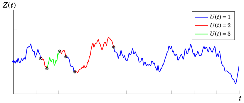
Figure 1. This figure shows a realization $A=(U,Z)$. The $y$-axis represents the output of $Z$, and the colors represent the value of the process $U$ (the jump times $\tau_{k}$ therein are represented by the symbol $\otimes$).

Let $U(t)$ and $\tau_{k}$ be as in Definition 1.11 (i.e., uniform continuous-time random walk on the complete graph with vertices $\{1,\ldots,r\}$ with jump rate $(r-1)$). We define the Markov process $A(t)=\big{(}U(t),Z(t)\big{)}$, assuming that $U$ and $Z$ are independent. See Figure 1 for an illustration of $A$’s path, which takes values in $\mathcal{A}$.

In Cases 2 and 3, for every $1\leq i\leq r$, $c\in\partial I$, and $0\leq s\leq t$, we define

(3.2) $$\mathfrak{L}^{(i,c)}_{[s,t)}(A)=\sum_{k\geq 1:~{}U(\tau_{k-1})=i}\mathfrak{L}_{[\tau_{k-1},\tau_{k})\cap[s,t)}^{c}(Z);$$

i.e., $Z$’s boundary local time at $c$ restricted to the subset $\{u\in[s,t):U(u)=i\}$. We note

$$\mathfrak{L}^{c}_{[s,t)}(Z)=\sum_{i=1}^{r}\mathfrak{L}^{(i,c)}_{[s,t)}(A).$$

However, we are more interested in the combination of these boundary local times weighted by the constants $\overline{\alpha}$ and $\overline{\beta}$ that determine the boundary conditions in Assumption 2.4, thus leading us to define the boundary term

(3.3) $$\mathfrak{B}_{t}(A)=\begin{cases}0&\text{Case 1,}\vspace{5pt}\\ \displaystyle\sum_{i=1}^{r}\overline{\alpha}_{i}\mathfrak{L}^{(i,0)}_{t}(A)&\text{Case 2,}\vspace{5pt}\\ \displaystyle\sum_{i=1}^{r}\overline{\alpha}_{i}\mathfrak{L}^{(i,0)}_{t}(A)+\sum_{i=1}^{r}\overline{\beta}_{i}\mathfrak{L}^{(i,\vartheta)}_{t}(A)&\text{Case 3.}\end{cases}$$

Finally, we state a general notation for random paths conditioned on their start and end points, which in the sequel will be applied to $U,Z,A,$ and other processes, as well as some notation for conditional expectations:

Definition 3.3.

Let $\mathfrak{X}=\big{(}\mathfrak{X}(t)\big{)}_{t\geq 0}$ be any continuous-time random process with càdlàg sample paths. We denote $\mathfrak{X}$’s transition kernel by

$$\Pi_{\mathfrak{X}}(t;x,y)=\begin{cases}\mathbf{P}[\mathfrak{X}(t)=y|\mathfrak{X}(0)=x]&\text{if $\mathfrak{X}$ is discrete,}\\ \mathbf{P}[\mathfrak{X}(t)\in\mathrm{d}y|\mathfrak{X}(0)=x]&\text{if $\mathfrak{X}$ is continuous.}\end{cases}$$

For any states $x,y$ and any time $t\geq 0$, we denote the conditionings

$$\mathfrak{X}^{x}=\big{(}\mathfrak{X}\big{|}\mathfrak{X}(0)=x\big{)}\qquad\text{and}\qquad\mathfrak{X}^{x,y}_{t}=\big{(}\mathfrak{X}\big{|}\mathfrak{X}(0)=x\text{ and }\mathfrak{X}(t)=y\big{)}.$$

Definition 3.4.

Given a random variable/process $\mathfrak{X}$ and a functional $F(\mathfrak{X})$ that may depend on other sources of randomness, we let $\mathbf{E}{{}_{\mathfrak{X}}}\big{[}F(\mathfrak{X})\big{]}$ denote the expectation with respect to $\mathfrak{X}$ only, conditional on any other source of randomness.

3.2. Regular Feynman-Kac Formula

Theorem 3.5.

Let Assumptions 2.3, 2.4, and 2.8 hold, assuming further that each entry $\xi_{i,j}$ is a regular noise in the sense of Definition 2.6. To simplify our notation, let us write $V+\xi$’s diagonal part as

$$S(i,x)=V(i,x)+\xi_{i,i}(x),\qquad 1\leq i\leq r,~{}x\in I,$$

and the non-diagonal part as

$$Q_{i,j}(x)=\xi_{i,j}(x),\qquad 1\leq i\neq j\leq r,~{}x\in I.$$

Denote the functional

(3.4) $$\mathfrak{n}_{t}(Q,A)=\begin{cases}\mathrm{e}^{(r-1)t}&\text{if }N(t)=0,\\ \displaystyle\mathrm{e}^{(r-1)t}(-1)^{N(t)}\left(\prod_{k=1}^{N(t)}\xi_{J_{k}}\big{(}Z(\tau_{k})\big{)}\right)&\text{if }N(t)>0,\end{cases}$$

where we recall that $N(t)$, $\tau_{k}$, and $J_{k}$ were introduced in Definition 1.11. Given $t>0$, let $\widehat{K}(t)$ be the random integral operator on $L^{2}(\mathcal{A},\mathbb{F})$ with kernel

(3.5) $$\widehat{K}(t;a,b)=\Pi_{A}(t;a,b)\mathbf{E}_{A}\left[\mathfrak{n}_{t}(Q,A^{a,b}_{t})\,\mathrm{e}^{-\int_{0}^{t}S(A^{a,b}_{t}(s))~{}\mathrm{d}s+\mathfrak{B}_{t}(A^{a,b}_{t})}\right],\qquad a,b\in\mathcal{A}$$

(this is random because it depends on the realization of $\xi$ via $S$ and $Q$); i.e.,

$$\widehat{K}(t)f(a)=\int_{\mathcal{A}}\widehat{K}(t;a,b)f(b)~{}\mathrm{d}\mu(b),\qquad f\in L^{2}(\mathcal{A},\mathbb{F}).$$

Almost surely, for every $t>0$, one has

(3.6) $$\mathrm{e}^{-t\widehat{H}}=\widehat{K}(t)\qquad\text{and}\qquad\mathrm{Tr}\big{[}\mathrm{e}^{-t\widehat{H}}\big{]}=\int_{\mathcal{A}}\widehat{K}(t;a,a)~{}\mathrm{d}\mu(a)<\infty.$$

Before moving on, a few remarks:

Remark 3.6.

In (3.5), we use the conventions that $x-\infty=-\infty$ for all $x\in[-\infty,\infty)$, and that $\mathrm{e}^{-\infty}=0$. Thus, when one of the boundary conditions is Dirichlet (in the convention of Assumption 2.4, $\overline{\alpha}_{i}=-\infty$ and/or $\overline{\beta}_{i}=-\infty$ for some $1\leq i\leq r$), its contribution to the boundary term $\mathfrak{B}_{t}(A)$ defined in (3.3) is interpreted as

$$\mathrm{e}^{-\infty\mathfrak{L}^{(i,c)}_{t}(Z)}=\mathbf{1}_{\{\mathfrak{L}^{(i,c)}_{t}(Z)=0\}}=\mathbf{1}_{\{Z(s)\neq c\text{ for every }s\in[0,t)\text{ such that }U(s)=i\}}.$$

Remark 3.7.

When $r=1$, the process $U(t)$ is just constant on $1$, and $\mathfrak{n}_{t}(Q,A)=1$. In this case, we can simply identify $\mathcal{A}=\{1\}\times I=I$, and Theorem 3.5 reduces to the one-dimensional Feynman-Kac formula for $Hf=-\frac{1}{2}f^{\prime\prime}+Sf$, with $S(x)=V(x)+\xi(x)$:

(3.7) $$\widehat{K}(t;x,y)=\begin{cases}\Pi_{B}(t;x,y)\mathbf{E}_{A}\left[\mathrm{e}^{-\int_{0}^{t}S(B^{x,y}_{t}(s))~{}\mathrm{d}s}\right]&\text{Case 1,}\vspace{5pt}\\ \Pi_{X}(t;x,y)\mathbf{E}_{A}\left[\mathrm{e}^{-\int_{0}^{t}S(X^{x,y}_{t}(s))~{}\mathrm{d}s+\overline{\alpha}\mathfrak{L}^{0}_{t}(X^{x,y}_{t})}\right]&\text{Case 2,}\vspace{5pt}\\ \Pi_{Y}(t;x,y)\mathbf{E}_{A}\left[\mathrm{e}^{-\int_{0}^{t}S(Y^{x,y}_{t}(s))~{}\mathrm{d}s+\overline{\alpha}\mathfrak{L}^{0}_{t}(Y^{x,y}_{t})+\overline{\beta}\mathfrak{L}^{\vartheta}_{t}(Y^{x,y}_{t})}\right]&\text{Case 3.}\end{cases}$$

See, e.g., [10, 48, 55] (more precise references can be found in Section 6.2.1).

Remark 3.8.

Looking back at (3.1), we can informally write

(3.8) $$\mathfrak{L}^{c}_{[s,t)}(Z)=\frac{1}{2}\int_{s}^{t}\delta_{c}\big{(}Z(u)\big{)}~{}\mathrm{d}u,$$

where $\delta_{c}$ denotes the delta Dirac mass at $c\in\{0,\vartheta\}$. Thus, the presence of the boundary terms (i.e., the multiples of $\mathfrak{L}_{t}^{c}(Z)$) in the scalar Feynman-Kac formula (3.7) in Cases 2 and 3 can be explained by the following heuristic: The process of going from the scalar full-space Feynman-Kac formula to the half-line or interval involves

1. replacing $B$ by the appropriate reflected version $X$ or $Y$, and

2. replacing $V(x)$ by $V(x)-\frac{\overline{\alpha}}{2}\delta_{0}(x)$ in Case 2 or $V(x)-\frac{\overline{\alpha}}{2}\delta_{0}(x)-\frac{\overline{\beta}}{2}\delta_{\vartheta}(x)$ in Case 3.

(This heuristic can also be justified by examining the quadratic forms of the operators involved; see Definition 2.11.) In the vector-valued case, we can explain the presence of the boundary term $\mathfrak{B}_{t}(Z)$ in (3.5) by performing the same heuristic; the only difference is that we replace the entries of the matrix potential $V+\xi=S+Q$ by

(3.9) $$\begin{cases}S(i,x)-\frac{\overline{\alpha}_{i}}{2}\delta_{0}(x)&\text{if }i=j\\ Q_{i,j}(x)&\text{if }i\neq j\end{cases}\qquad\text{or}\qquad\begin{cases}S(i,x)-\frac{\overline{\alpha}_{i}}{2}\delta_{0}(x)-\frac{\overline{\beta}_{i}}{2}\delta_{\vartheta}(x)&\text{if }i=j\\ Q_{i,j}(x)&\text{if }i\neq j\end{cases}$$

in Cases 2 or 3 respectively. By Proposition 1.12, we understand that the contribution of $V+\xi$’s diagonal to $\overrightarrow{\mathcal{T}}\left\{\mathrm{e}^{-\int_{0}^{t}V(Z(s))+\xi(Z(s))}\right\}$ is in the exponential $\mathrm{e}^{-\int_{0}^{t}S(A(s))~{}\mathrm{d}s}$; hence (3.9) very naturally leads to $\mathfrak{B}_{t}(Z)$. In contrast, the contributions of the Dirac masses in (3.9) are arguably more difficult to parse/calculate if we use either (1.12), (1.16), or (1.17) to write the operator exponentials.

4. Main Results Part 3. Trace Moments and Rigidity

We now finish the statements of our main results with the Feynman-Kac formulas for the trace moments (1.2), as well as our rigidity result.

4.1. Combinatorial and Stochastic Process Preliminaries

We begin by introducing the combinatorial objects that are used to characterize which jump sequences $J_{1},J_{2},J_{3},\ldots$ in the process $U$ contribute to the sum (1.25) (the latter of which we recall arises from an application of Isserlis’ theorem):

Definition 4.1.

Given $n\in\mathbb{N}$, let $\mathcal{B}_{n}$ denote the set of binary sequences with $n$ steps, namely, sequences of the form $m=(m_{0},m_{1},\ldots,m_{n})\in\{0,1\}^{n+1}$. Given $h,l\in\{0,1\}$, we let $\mathcal{B}^{h,l}_{n}$ denote the set of sequences $m\in\mathcal{B}_{n}$ such that $m_{0}=h$ and $m_{n}=l$.

Definition 4.2.

Suppose we are given a realization of the process $U$ in Definition 3.2. Let $t\geq 0$ be fixed, and suppose that $N(t)\geq 2$ is even. Given any jump $J_{k}=(i,j)$, we let $J_{k}^{*}=(j,i)$ denote that same jump in reverse order. Given any matching $p\in\mathcal{P}_{N(t)}$ (recall Definition 1.14), we define the constant $\mathfrak{C}_{t}(p,U)$ as follows:

1. If $\mathbb{F}=\mathbb{R}$, then

   $$\mathfrak{C}_{t}(p,U)=\begin{cases}1&\text{if either $J_{\ell_{1}}=J_{\ell_{2}}$ or $J_{\ell_{1}}=J_{\ell_{2}}^{*}$ for all $\{\ell_{1},\ell_{2}\}\in p$},\\ 0&\text{otherwise}.\end{cases}$$

2. If $\mathbb{F}=\mathbb{C}$, then

   $$\mathfrak{C}_{t}(p,U)=\begin{cases}1&\text{if $J_{\ell_{1}}=J_{\ell_{2}}^{*}$ for all $\{\ell_{1},\ell_{2}\}\in p$},\\ 0&\text{otherwise}.\end{cases}$$

3. If $\mathbb{F}=\mathbb{H}$, then

   $$\mathfrak{C}_{t}(p,U)=\begin{cases}\mathfrak{D}_{t}(p,U)&\text{if either $J_{\ell_{1}}=J_{\ell_{2}}$ or $J_{\ell_{1}}=J_{\ell_{2}}^{*}$ for all $\{\ell_{1},\ell_{2}\}\in p$},\\ 0&\text{otherwise}.\end{cases}$$

   Here, we define $\mathfrak{D}_{t}(p,U)$ as follows: A binary sequence $m\in\mathcal{B}^{0,0}_{N(t)}$ is said to respect $(p,J)$ if for every pair $\{\ell_{1},\ell_{2}\}\in p$, the following holds:

   1. if $J_{\ell_{1}}=J_{\ell_{2}}$, then $\big{(}(m_{\ell_{1}-1},m_{\ell_{1}}),(m_{\ell_{2}-1},m_{\ell_{2}})\big{)}$ are equal to one of the following pairs: $\big{(}(0,0),(1,1)\big{)}$, $\big{(}(1,1),(0,0)\big{)}$, $\big{(}(0,1),(1,0)\big{)}$, or $\big{(}(1,0),(0,1)\big{)}$.

   2. if $J_{\ell_{1}}=J_{\ell_{2}}^{*}$, then $\big{(}(m_{\ell_{1}-1},m_{\ell_{1}}),(m_{\ell_{2}-1},m_{\ell_{2}})\big{)}$ are equal to one of the following pairs: $\big{(}(0,0),(0,0)\big{)}$, $\big{(}(1,1),(1,1)\big{)}$, $\big{(}(0,1),(1,0)\big{)}$, or $\big{(}(1,0),(0,1)\big{)}$.

   Lastly, we call any pair $\{\ell_{1},\ell_{2}\}\in p$ such that $J_{\ell_{1}}=J_{\ell_{2}}$ and

   $$\big{(}(m_{\ell_{1}-1},m_{\ell_{1}}),(m_{\ell_{2}-1},m_{\ell_{2}})\big{)}=\big{(}(0,1),(1,0)\big{)}\text{ or }\big{(}(1,0),(0,1)\big{)}$$

   a flip, and we let $f(m,p,J)$ denote the total number of flips that occur in the combination of $m,p,$ and $J$. With all this in hand, we finally define

   (4.1) $$\mathfrak{D}_{t}(p,U)=2^{-N(t)/2}\sum_{m\in\mathcal{B}^{0,0}_{N(t)},~{}m\text{ respects }(p,J)}(-1)^{f(m,p,J)}.$$

Remark 4.3.

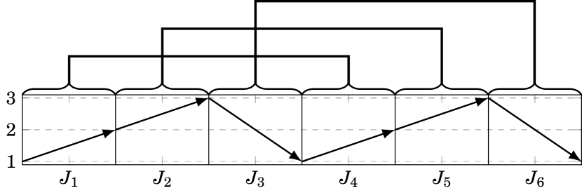
Figure 3. In this figure, the arrows represent the first six jumps of $U$ by time $t$, namely, $(1,2),(2,3),(3,1),(1,2),(2,3),(3,1)$. The partition above the arrows serve to highlight which jumps were paired by the perfect matching $p=\big{\{}\{1,4\},\{2,5\},\{3,6\}\big{\}}$. With this in hand, we conclude that this particular combination of $(p,U)$ is such that $\mathfrak{C}_{t}(p,U)\neq 0$ when $\mathbb{F}=\mathbb{R},\mathbb{H}$, since $J_{1}=J_{4}$, $J_{2}=J_{5}$, and $J_{3}=J_{6}$. However, $\mathfrak{C}_{t}(p,U)=0$ when $\mathbb{F}=\mathbb{C}$ because paired jumps are not reversed.

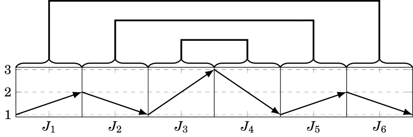
Figure 4. In this figure, the six jumps by time $t$ are $(1,2),(2,1),(1,3),(3,1),(1,2),(2,1)$, and $p=\big{\{}\{1,6\},\{2,5\},\{3,4\}\big{\}}$. In this case, $\mathfrak{C}_{t}(p,U)\neq 0$ for all $\mathbb{F}=\mathbb{R},\mathbb{C},\mathbb{H}$, since every paired jumps are reversed (i.e., $J_{1}=J_{6}^{*}$, $J_{2}=J_{5}^{*}$, and $J_{3}=J_{4}^{*}$).

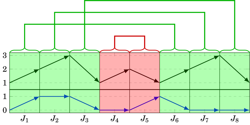
Figure 5. In this figure, the black arrows are the steps $J_{k}$ until $N(t)$, the blue arrows are the steps of a binary sequence $m\in\mathcal{B}^{0,0}_{N(t)}$, and the partition above all that represents the pairs given by $p$. In order to help decipher whether this choice of $m$ contributes to $\mathfrak{D}_{t}(p,U)$, the matched pairs of steps such that $J_{\ell_{1}}=J_{\ell_{2}}$ are colored in green, and the matched pairs such that $J_{\ell_{1}}=J_{\ell_{2}}^{*}$ are colored in red. In this case, $m$ does not respect $(p,J)$, and thus it does not contribute to $\mathfrak{D}_{t}(p,U)$. (E.g., $J_{4}$ and $J_{5}$ are matched and in opposite directions, but the corresponding steps in the binary sequence, $\big{(}(0,0),(0,1)\big{)}$, are not among those listed in Definition 4.2-(3.2))

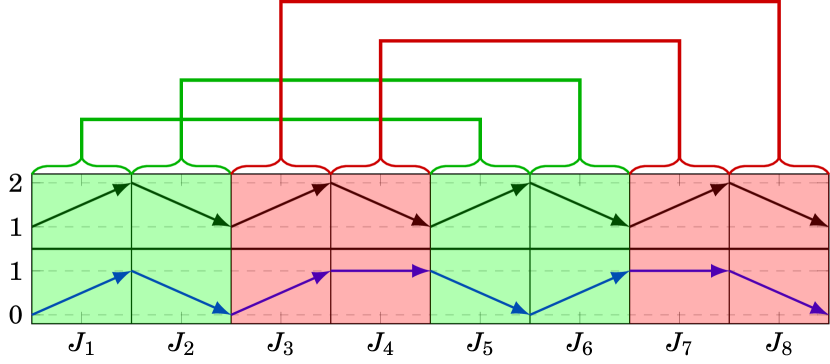
Figure 7. This is another example where $m$ contributes to $\mathfrak{D}_{t}(p,U)$. Moreover, in this case we have $f(m,p,J)=2$; the two flips occur at the pairs $J_{1},J_{5}$ and $J_{2},J_{6}$.

We refer to Figures 3, 4, 5, 6, and 7 in Appendix A for illustrations of the objects related to the combinatorial constants in Definition 4.2. Moreover, we note that for any $p\in\mathcal{P}_{N(t)}$, the number of binary paths that respect $(p,J)$ is at most $2^{N(t)/2}$ (since every step $(m_{\ell_{1}-1},m_{\ell_{1}})$ determines the other step $(m_{\ell_{2}-1},m_{\ell_{2}})$ that is matched to it via $\{\ell_{1},\ell_{2}\}\in p$). Consequently, in all cases (i.e., for $\mathbb{F}=\mathbb{R},\mathbb{C},\mathbb{H}$), one has

(4.2) $$|\mathfrak{C}_{t}(p,U)|\leq 1.$$

Next, in order to formalize the singular conditioning on the event (1.26), we introduce self-intersection local time measures induced by a permutation, the latter of which require a precise definition of local time processes:

Definition 4.4.

Let $\big{(}L^{x}_{[s,t)}(Z):0\leq s<t,~{}x\in I\big{)}$ denote the continuous (jointly in $s$, $t$, and $x$) version of $Z$’s local time process on the time intervals $[s,t)$, that is,

(4.3) $$\int_{s}^{t}f\big{(}Z(u)\big{)}~{}\mathrm{d}u=\int_{I}L^{x}_{[s,t)}(Z)f(x)~{}\mathrm{d}x\qquad\text{for all measurable }f:I\to\mathbb{R}.$$

(see, e.g., [54, 5, Chapter VI, Corollary 1.6 and Theorem 1.7] for a proof of the existence of this continuous version). We use the convention $L_{t}^{x}(Z)=L_{[0,t)}^{x}(Z)$.

Next, we define the local time process $\big{(}L_{[s,t)}^{a}(A):0\leq s<t,~{}a\in\mathcal{A}\big{)}$ of the multivariate process $A=(U,Z)$ as follows:

(4.4) $$L^{(i,x)}_{[s,t)}(A)=\sum_{k\geq 1:~{}U(\tau_{k-1})=i}L_{[\tau_{k-1},\tau_{k})\cap[s,t)}^{x}(Z);$$

$$\int_{s}^{t}f\big{(}A(u)\big{)}~{}\mathrm{d}u=\sum_{k\geq 1}\int_{[\tau_{k-1},\tau_{k})\cap[s,t)}f\big{(}U(\tau_{k-1}),Z(u)\big{)}~{}\mathrm{d}u=\int_{\mathcal{A}}L^{a}_{[s,t)}(A)f(a)~{}\mathrm{d}\mu(a).$$

In particular, for every $0\leq s<t$ and $x\in I$, one has

(4.5) $$\sum_{i=1}^{r}L^{(i,x)}_{[s,t)}(A)=L^{x}_{[s,t)}(Z).$$

Finally, let $t>0$, let $n\geq 2$ be an even integer, and let $q\in\mathcal{P}_{n}$. Given a realization of $Z$, we let $\mathrm{si}_{t,n,q,Z}$ denote the unique random Borel probability measure on $[0,t)^{n}$ such that for every $s_{1},t_{1},\ldots,s_{n},t_{n}\in[0,t)$ with $s_{k}<t_{k}$ for $k=1,\ldots,n$, one has

(4.6) $$\mathrm{si}_{t,n,q,Z}\big{(}[s_{1},t_{1})\times[s_{2},t_{2})\times\cdots\times[s_{n},t_{n})\big{)}\\ =\frac{1}{\|L_{t}(Z)\|_{2}^{2n}}\prod_{\{\ell_{1},\ell_{2}\}\in q}\left\langle L_{[s_{\ell_{1}},t_{\ell_{1}})}(Z),L_{[s_{\ell_{2}},t_{\ell_{2}})}(Z)\right\rangle$$

(this uniquely determines the measure since product rectangles are a determining class for the Borel $\sigma$-algebra).

Remark 4.5.

Informally, one can think of $\mathrm{si}_{t,n,q,Z}$ as the uniform probability measure on the set of $n$-tuples of time coordinates in $[0,t)^{n}$ such that each pair of times matched by $q$ coincide with a self-intersection of $Z$; namely:

$$\big{\{}(t_{1},\ldots,t_{n})\in[0,t)^{n}:Z(t_{\ell_{1}})=Z(t_{\ell_{2}})\text{ for all }\{\ell_{1},\ell_{2}\}\in q\big{\}}.$$

(We point to [7, Theorem 2.3.2 and Proposition 2.3.5] for a proof that $\mathrm{si}_{t,n,q,Z}$ is supported on that set.) Recall that, conditional on $N(t)$, the jump times $\tau_{1},\ldots,\tau_{N(t)}$ are the order statistics of i.i.d. uniform random variables in $[0,t)$. Thus, $\mathrm{si}_{t,n,q,Z}$ serves as a natural means of formalizing the conditioning on the event (1.26) (assuming $q$ and the matching $p$ in (1.26) are related to each other in such a way that $p$ matches the same pairs of times $t_{k}$ as $q$ once they are arranged in nondecreasing order).

Finally, given that products of Feynman-Kac kernels involve multiple independent copies of the processes $U$ and $X$, we introduce some notation to help write such expressions tidily:

Definition 4.6.

Let $\mathfrak{X}$ be a stochastic process with càdlàg sample paths. Given $n$-tuples of times $\boldsymbol{t}=(t_{1},\ldots,t_{n})$ and states $\boldsymbol{x}=(x_{1},\ldots,x_{n})$, we let

(4.7) $$\mathfrak{X}^{\boldsymbol{x}}_{\boldsymbol{t}}=\mathfrak{X}^{(x_{1},\ldots,x_{n})}_{(t_{1},\ldots,t_{n})}$$

denote a càdlàg concatenation of independent paths

$$\big{(}\mathfrak{X}^{x_{1}}(s):s\in[0,t_{1})\big{)},\big{(}\mathfrak{X}^{x_{2}}(s):s\in[0,t_{2})\big{)},\ldots,\big{(}\mathfrak{X}^{x_{n}}(s):s\in[0,t_{n})\big{)}$$

on the time-interval $[0,t_{1}+\cdots+t_{k})$. That is, to generate $\mathfrak{X}^{\boldsymbol{x}}_{\boldsymbol{t}}(s)$, we follow the steps:

1. firstly, we run a path of $\mathfrak{X}$ started at $x_{1}$ on the time interval $[0,t_{1})$;

2. secondly, we run an independent path of $\mathfrak{X}$ started at $x_{2}$ on the time interval $[t_{1},t_{1}+t_{2})$;

3. $\cdots$

4. lastly, we run an independent path of $\mathfrak{X}$ started at $x_{n}$ on the time interval $[t_{1}+\cdots+t_{n-1},t_{1}+\cdots+t_{n})$.

Given $n$-tuples of times $\boldsymbol{t}=(t_{1},\ldots,t_{n})$ and states $\boldsymbol{x}=(x_{1},\ldots,x_{n})$, $\boldsymbol{y}=(y_{1},\ldots,y_{n})$, let

(4.8) $$\mathfrak{X}^{\boldsymbol{x},\boldsymbol{y}}_{\boldsymbol{t}}=\mathfrak{X}^{(x_{1},\ldots,x_{n}),(y_{1},\ldots,y_{n})}_{(t_{1},\ldots,t_{n})}$$

be the càdlàg concatenation $\mathfrak{X}^{\boldsymbol{x}}_{\boldsymbol{t}}$ with the additional endpoint conditioning

$$\mathfrak{X}^{\boldsymbol{x},\boldsymbol{y}}_{\boldsymbol{t}}=\left(\mathfrak{X}^{\boldsymbol{x}}_{\boldsymbol{t}}~{}\bigg{|}~{}\lim_{s\to(t_{1}+\cdots+t_{k})^{-}}\mathfrak{X}^{\boldsymbol{x}}_{\boldsymbol{t}}(s)=y_{k}\text{ for all }1\leq k\leq n\right).$$

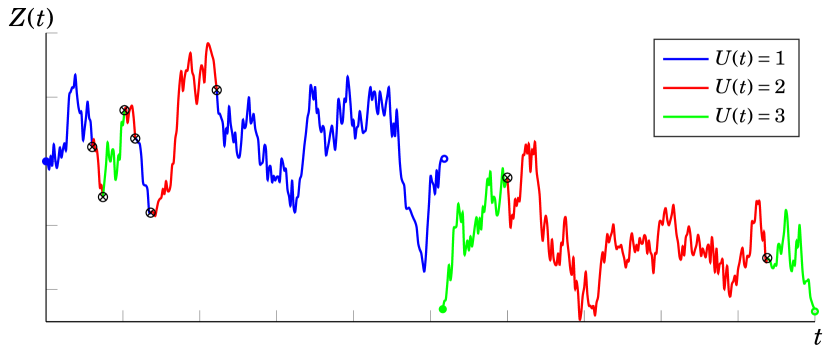
Figure 2. This figure shows a realization of the càdlàg concatenated path $A^{\boldsymbol{a},\boldsymbol{b}}_{\boldsymbol{t}}$ with $\boldsymbol{a}=\big{(}(1,1),(3,0)\big{)}$, $\boldsymbol{b}=\big{(}(1,1),(3,0)\big{)}$, and $\boldsymbol{t}=(1,1)$ (i.e., the first path goes from $(i,x)=(1,1)$ to itself in time $1$, and the second path goes from $(i,x)=(3,0)$ to itself in time $1$).

See Figure 2 for an illustration of one such càdlàg concatenation in the case $\mathfrak{X}=A$. Finally, we use the following shorthand for a product of transition kernels:

$$\Pi_{\mathfrak{X}}(\boldsymbol{t};\boldsymbol{x},\boldsymbol{y})=\prod_{k=1}^{n}\Pi_{\mathfrak{X}}(t_{k};x_{k},y_{k}).$$

4.2. Trace Moment Formulas

We are now finally in a position to state our trace moment formulas in the case where $\xi$ is a white noise. First, we provide a precise statement of how the conditioning on the singular event (1.26) is achieved:

Definition 4.7.

Suppose that we are given a realization of $Z$ on some time interval $[0,t)$. Given this, we generate the process $\widehat{U}$ on $[0,t)$ as follows:

1. Given $Z$, sample $\widehat{N}(t)$ according to the distribution

   $$\mathbf{P}\big{[}\widehat{N}(t)=2m\big{]}=\left(\frac{\big{(}(r-1)^{2}\|L_{t}(Z)\|^{2}_{2}}{2}\right)^{m}\frac{1}{m!}\mathrm{e}^{-\frac{(r-1)^{2}}{2}\|L_{t}(Z)\|_{2}^{2}},\qquad m=0,1,2,\ldots,$$

   i.e., $\widehat{N}(t)/2$ is Poisson with parameter $\frac{(r-1)^{2}}{2}\|L_{t}(Z)\|_{2}^{2}$.

2. Given $\widehat{N}(t)$, sample $\widehat{q}$ uniformly at random in $\mathcal{P}_{\widehat{N}(t)}$.

3. Given $Z$, $\widehat{N}(t)$, and $\widehat{q}$, draw $\boldsymbol{T}=(T_{1},\ldots,T_{\widehat{N}(t)})\in[0,t]^{\widehat{N}(t)}$ according to the self-intersection measure $\mathrm{si}_{t,\widehat{N}(t),\widehat{q},Z}$. Then, recalling the notation of Theorem 1.10-(2), we define $\widehat{\boldsymbol{\tau}}=(\widehat{\tau}_{1},\ldots,\widehat{\tau}_{\widehat{N}(t)})$ to be such that $\widehat{\tau}_{k}=\overrightarrow{T_{k}}$ for all $k\geq 1$. In words, $\widehat{\boldsymbol{\tau}}$ is the tuple $\boldsymbol{T}$ rearranged in nondecreasing order.

4. Given $\widehat{N}(t)$, $\boldsymbol{T}$, and $\widehat{\boldsymbol{\tau}}$, we let $\widehat{\pi}$ be the random permutation of $\{1,\ldots,\widehat{N}(t)\}$ such that $\widehat{\tau}_{\widehat{\pi}(\ell)}=T_{\ell}$ for all $\ell\leq\widehat{N}(t)$, and we let $\widehat{p}\in\mathcal{P}_{\widehat{N}(t)}$ be the random perfect matching such that $\{\ell_{1},\ell_{2}\}\in\widehat{q}$ if and only if $\{\widehat{\pi}(\ell_{1}),\widehat{\pi}(\ell_{2})\}\in\widehat{p}$. In words, $\widehat{p}$ ensures that each pair of times $T_{k}$ that were matched by $\widehat{q}$ are still matched once arranged in nondecreasing order $\widehat{\tau}_{k}$.

5. Sample the jumps $J_{k}$ in the same way as for $U$, i.e., uniform random walk on the complete graph (without self-edges) on $\{1,\ldots,r\}$.

6. Combining all of the above, we then let $\big{(}\widehat{U}(s):1\leq s\leq t\big{)}$ be the càdlàg path with jump times $\widehat{\boldsymbol{\tau}}$ and jumps $J$ (in particular, if $\widehat{N}(t)=0$, then $\widehat{U}(t)$ is constant).

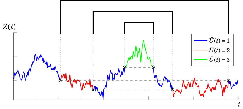
Figure 8. In this figure, the colored path represents a realization of $(\widehat{U},Z)$ with $Z(0)=1=Z(1)$. The symbols $\otimes$ along the path represent the jump times $\widehat{\tau}_{k}$, and the different colors represent the values of the process $\widehat{U}(t)$. The jumps $J_{k}$ and the random matching $\widehat{\pi}(P)$ (the latter of which is represented by the partition above $Z$’s path) are the same as $J_{k}$ and $p$ in Figure 4. In this illustration, we observe that $Z(\widehat{\tau}_{\ell_{1}})=Z(\widehat{\tau}_{\ell_{2}})$ for every matched pair $\{\ell_{1},\ell_{2}\}\in\widehat{\pi}(P)$, which is consistent with the fact that the pairs $\widehat{\tau}_{\ell_{1}}$ and $\widehat{\tau}_{\ell_{2}}$ were sampled according to $Z$’s self-intersection measure.

See Figure 8 for an illustration of $(\widehat{U},Z)$

Our trace moment formulas are as follows:

Theorem 4.8.

Let Assumptions 2.3, 2.4, and 2.8 hold, assuming further that $\xi_{i,i}$ are white noises in $\mathbb{R}$ with variance $\sigma^{2}>0$, and that $\xi_{i,j}$ ($i\neq j$) are white noises in $\mathbb{F}$ with variance $\upsilon^{2}>0$. Define the functionals

$$\mathfrak{M}_{t}(\widehat{p},\widehat{U})=\begin{cases}1&\text{if }\widehat{N}(t)=0\\ \upsilon^{\widehat{N}(t)}\mathfrak{C}_{\widehat{N}(t)}(\widehat{p},J)&\text{otherwise},\end{cases}$$

and

(4.9) $$\mathfrak{H}_{t}(\widehat{U},Z)=\frac{(r-1)^{2}\upsilon^{2}}{2}\|L_{t}(Z)\|_{2}^{2}+\frac{\sigma^{2}}{2}\|L_{t}(\widehat{U},Z)\|_{\mu}^{2}-\int_{0}^{|\boldsymbol{t}|}V\big{(}\widehat{U}(s),Z(s)\big{)}~{}\mathrm{d}s+\mathfrak{B}_{t}(\widehat{U},Z).$$

For every $\boldsymbol{t}=(t_{1},\ldots,t_{n})\in(0,\infty)^{n}$, one has

(4.10) $$\mathbf{E}\left[\mathrm{Tr}\big{[}\mathrm{e}^{-t_{1}\widehat{H}}\big{]}\cdots\mathrm{Tr}\big{[}\mathrm{e}^{-t_{n}\widehat{H}}\big{]}\right]\\ =\int_{\mathcal{A}^{n}}\Pi_{Z}(\boldsymbol{t};\boldsymbol{x},\boldsymbol{x})\mathbf{E}\left[\mathfrak{M}_{|\boldsymbol{t}|}(\widehat{p},\widehat{U}^{\boldsymbol{i}}_{\boldsymbol{t}})\mathrm{e}^{\mathfrak{H}_{|\boldsymbol{t}|}(\widehat{U}^{\boldsymbol{i}}_{\boldsymbol{t}},Z^{\boldsymbol{x},\boldsymbol{x}}_{\boldsymbol{t}})}\mathbf{1}_{\{\forall k:~{}\widehat{U}^{\boldsymbol{i}}_{\boldsymbol{t}}(t_{1}+\cdots+t_{k-1}+s)\to i_{k}\text{ as }s\to t_{k}^{-}\}}\right]~{}\mathrm{d}\mu^{n}(\boldsymbol{i},\boldsymbol{x}),$$

where we denote $\boldsymbol{i}=(i_{1},\ldots,i_{n})\in\{1,\ldots,r\}^{n}$ and $\boldsymbol{x}=(x_{1},\ldots,x_{n})\in I^{n}$.

4.3. Rigidity

We now state our result regarding the number rigidity of $\widehat{H}$. For this purpose, we recall the general formal definition of point processes on the real line:

Definition 4.9.

Let $\mathcal{K}\subset\mathbb{R}$ be a Borel set and $\mathcal{B}_{\mathcal{K}}$ be the $\sigma$-algebra of all Borel subsets of $\mathcal{K}$. Let $\mathcal{N}^{\#}_{\mathcal{K}}$ denote the set of integer-valued measures $\mathcal{M}$ on $(\mathcal{K},\mathcal{B}_{\mathcal{K}})$ such that $\mathcal{M}(\overline{\mathcal{K}})<\infty$ for every bounded set $\overline{\mathcal{K}}\in\mathcal{B}_{\mathcal{K}}$. We equip $\mathcal{N}^{\#}_{\mathcal{K}}$ with the topology generated by the maps

$$\mathcal{M}\mapsto\int f(x)~{}\mathrm{d}\mathcal{M}(x),\qquad f:\mathcal{K}\to\mathbb{R}\text{ is continuous and compactly supported,}$$

as well as the associated Borel $\sigma$-algebra. We note that for every $\mathcal{M}\in\mathcal{N}^{\#}_{\mathcal{K}}$, there exists a sequence $(x_{k})_{k\in\mathbb{N}}\subset\mathcal{K}$ without accumulation point such that $\mathcal{M}=\sum_{k=1}^{\infty}\delta_{x_{k}}$; i.e., $\mathcal{M}(\overline{\mathcal{K}})$ counts the number of points in the sequence $x_{k}$ that are within the set $\overline{\mathcal{K}}$. Finally, a point process on $\mathcal{K}$ is a random element that takes values in $\mathcal{N}^{\#}_{\mathcal{K}}$.

In this paper, we are only interested in the eigenvalue point process of $\widehat{H}$:

Definition 4.10.

Let Assumptions 2.3, 2.4, and 2.8 hold. We define $\widehat{H}$’s eigenvalue point process as

$$\widehat{\mathcal{M}}=\sum_{k=1}^{\infty}\delta_{\lambda_{k}(\widehat{H})}\in\mathcal{N}^{\#}_{\mathbb{R}}.$$

For every Borel set $\mathcal{K}\subset\mathbb{R}$, we denote the restriction

$$\widehat{\mathcal{M}}|_{\mathcal{K}^{c}}:=\sum_{k=1}^{\infty}\mathbf{1}_{\{\lambda_{k}(\widehat{H})\in\mathcal{K}^{c}\}}\,\delta_{\lambda_{k}(\widehat{H})}\in\mathcal{N}^{\#}_{\mathcal{K}^{c}}.$$

That is, the same random measure as $\widehat{\mathcal{M}}$, but excluding the masses in $\mathcal{K}$.

The definition of number rigidity used in this paper is as follows:

Definition 4.11.

We say that a Borel set $\mathcal{K}\subset\mathbb{R}$ is bounded above if there exists some $c\in\mathbb{R}$ such that $\mathcal{K}\subset(-\infty,c]$. (Note that by Proposition 2.14, $\widehat{\mathcal{M}}$ is such that, almost surely, $\mathcal{\widehat{M}}(\mathcal{K})<\infty$ for every Borel set $\mathcal{K}\subset\mathbb{R}$ that is bounded above.) We say that $\widehat{\mathcal{M}}$ is number rigid if for every bounded above Borel set $\mathcal{K}\subset\mathbb{R}$, there exists a deterministic measurable function $F_{\mathcal{K}}:\mathcal{N}^{\#}_{\mathcal{K}^{c}}\to\mathbb{R}$ such that

(4.11) $$\widehat{\mathcal{M}}(\mathcal{K})=F_{\mathcal{K}}\big{(}\widehat{\mathcal{M}}|_{B^{c}}\big{)}\qquad\text{almost surely};$$

in words, the number of eigenvalues in $\mathcal{K}$ is a deterministic function of the configuration of eigenvalues outside $\mathcal{K}$.

Our result regarding number rigidity is as follows:

Theorem 4.12.

Let Assumptions 2.3, 2.4, and 2.8 hold, assuming further that each entry of $\xi$ is a white noise.

1. In Cases 1 and 2, if there exists $\kappa,\nu>0$ such that $V(i,x)\geq\kappa|x|-\nu$ for all $1\leq i\leq r$ and $x\in I$, then $\widehat{\mathcal{M}}$ is number rigid. In particular, the eigenvalue point process of any multivariate SAO (as defined in Remark 2.10) is number rigid.

2. In Case 3, $\widehat{\mathcal{M}}$ is number rigid with no further condition on $V$.

5. Proof Roadmap

5.1. Proof of Proposition 2.14: Construction of Operators

Suppose that the assumptions in the statement of Proposition 2.14 hold. In the argument that follows, we record (as remarks) a few properties of the operators $H$ and $\widehat{H}$ that are not part of the statement of Proposition 2.14, but which are nevertheless important in the proofs of other results. Moreover, following-up on the Hilbert-space subtlety mentioned in Remark 2.2, we deal with the real/complex and quaternion cases separately throughout this section.

5.1.1. The Cases $\mathbb{F}=\mathbb{R},\mathbb{C}$

Assume first that $\mathbb{F}=\mathbb{R},\mathbb{C}$. We begin by constructing the deterministic operator $H$. For this purpose, for each $1\leq i\leq r$, recall the definition of $\mathcal{E}_{i}$ and $D(\mathcal{E}_{i})$ in Definition 2.11. By [26, Proposition 3.2], the operators $H_{i}$ defined in (2.7) are the unique self-adjoint operators with dense domains $D(H_{i})\subset D(\mathcal{E}_{i})\subset L^{2}(I,\mathbb{F})$ such that $\langle f,H_{i}g\rangle=\mathcal{E}_{i}(f,g)$ for all $f,g\in D(H_{i})$ (in [26], the result is stated for operators acting on real-valued functions, but the latter can be trivially extended to $\mathbb{C}$ or $\mathbb{F}$ by linearity). Moreover, each $H_{i}$ has compact resolvent.

Remark 5.1.

For $1\leq i\leq r$, let $\mathrm{FC}_{i}$ denote the set of functions $\varphi\in C_{0}^{\infty}(I,\mathbb{F})$ that satisfy the following:

1. $\varphi$ is supported inside $I$ in Case 1, as well as Cases 2 and 3 with Dirichlet boundary conditions (i.e., $\overline{\alpha}_{i}=-\infty$ in Case 2 and $\overline{\alpha}_{i}=\overline{\beta}_{i}=-\infty$ in Case 3).

2. $\varphi$ is supported inside $I$’s closure in Cases 2 and 3 with Robin boundary conditions (i.e., $\overline{\alpha}_{i},\overline{\beta}_{i}\in\mathbb{R}$).

3. In Case 3, $\varphi$ is supported in $[0,b)$ if $\overline{\alpha}_{i}\in\mathbb{R}$ and $\overline{\beta}_{i}=-\infty$, and $\varphi$ is supported in $(0,b]$ if $\overline{\alpha}_{i}=-\infty$ and $\overline{\beta}_{i}\in\mathbb{R}$.

In [26, Proposition 3.2], it is also proved that $\mathrm{FC}_{i}\subset D(\mathcal{E}_{i})$ is a form core for $\mathcal{E}_{i}$.

Remark 5.2.

In [26, Theorem 5.4 and Lemma 5.13], it is also proved that

$$\mathrm{Tr}\big{[}\mathrm{e}^{-tH_{i}}\big{]}=\sum_{k=1}^{\infty}\mathrm{e}^{-t\lambda_{k}(H_{i})}<\infty.$$

With this in hand, we can now define the operator

(5.1) $$Hf(i,x)=-\tfrac{1}{2}f^{\prime\prime}(i,x)+V(i,x)f(i,x),\qquad(i,x)\in\mathcal{A}$$

as the direct sum $H=H_{1}\oplus\cdots\oplus H_{r}$. By [51, Theorem XIII.85], $H$ self-adjoint on the domain $D(H)=D(H_{1})\oplus\cdots\oplus D(H_{r})$, which is dense in $L^{2}(\mathcal{A},\mathbb{F})$. Recalling the definition of $\mathcal{E}$ and $D(\mathcal{E})$ at the end of Definition 2.11, this means that $D(H)\subset D(\mathcal{E})$ and $\langle f,Hg\rangle_{\mu}=\mathcal{E}(f,g)$ for all $f,g\in D(H)$. Finally, we note that since each $H_{i}$ has compact resolvent, the same is true for $H$: Given that $H=H_{1}\oplus\cdots\oplus H_{r}$, the eigenvalue-eigenfunction pairs $\big{(}\lambda_{k}(H),\psi_{k}(H)\big{)}_{k\in\mathbb{N}}$ of $H$ are of the form

(5.2) $$\lambda_{k}(H)=\lambda_{\ell}(H_{i})\qquad\text{and}\qquad\psi_{k}(H)=0\oplus\cdots\oplus 0\oplus\psi_{\ell}(H_{i})\oplus 0\oplus\cdots\oplus 0,$$

for some $\ell\in\mathbb{N}$.

Remark 5.3.

If we combine Remark 5.2 with (5.2), then we get that

(5.3) $$\mathrm{Tr}\big{[}\mathrm{e}^{-tH}\big{]}=\sum_{k=1}^{\infty}\mathrm{e}^{-t\lambda_{k}(H)}=\sum_{i=1}^{r}\sum_{k=1}^{\infty}\mathrm{e}^{-t\lambda_{k}(H_{i})}<\infty.$$

With the construction of $H$ completed, we are now ready to wrap up the proof of Proposition 2.14. By Proposition 2.12, almost surely, $\xi$ is an infinitesimally form-bounded perturbation of $\mathcal{E}$. Thus, Proposition 2.14-(1) and -(2) follow directly from the KLMN theorem (e.g., [53, Theorem VIII.15] and [52, Theorem X.17]), and the fact that $\widehat{H}$ has compact resolvent follows from the fact that $H$ has compact resolvent and standard variational estimates (e.g., [51, Theorem XIII.68]).

Remark 5.4.

Another conclusion of the KLMN theorem is that any form core for $\mathcal{E}$ is also a form core for $\widehat{\mathcal{E}}$ (e.g., [56, Theorem 7.5.7]). Thus, following-up on Remark 5.1, $\mathrm{FC}=\mathrm{FC}_{1}\oplus\cdots\oplus\mathrm{FC}_{r}$ is a form core for both $\mathcal{E}$ and $\widehat{\mathcal{E}}$ (the latter almost surely).

5.1.2. The Case $\mathbb{F}=\mathbb{H}$

Consider now the case $\mathbb{F}=\mathbb{H}$. The results in [51, 52, 53, 56] that were cited in Section 5.1.1 require that $H_{i}$, $H$, and $\widehat{H}$ be defined on a standard real or complex Hilbert space. For this purpose, we first assume that $L^{2}(I,\mathbb{H})$ and $L^{2}(\mathcal{A},\mathbb{H})$ are equipped with the real inner products (2.1), and that the bilinear forms for $H_{i}$ and $H$ are replaced by

$$\mathcal{Q}_{i}(f,g)=\Re\big{(}\mathcal{E}_{i}(f,g)\big{)}\qquad\text{and}\qquad\mathcal{Q}(f,g)=\Re\big{(}\mathcal{E}(f,g)\big{)};$$

the quadratic form

$$\widehat{\mathcal{E}}(f,f)=\mathcal{Q}(f,f)+\Re\big{(}\xi(f,f)\big{)}=\mathcal{E}(f,f)+\xi(f,f)$$

does not need to be changed, as $\mathcal{E}(f,f)$ and $\xi(f,f)$ are always real. The argument in Section 5.1.1 then yields the conclusion of Proposition 2.14, the only difference being that, in the variational spectrum

(5.4) $$\Lambda_{\ell}(\widehat{H})=\inf_{f\in D(\mathcal{E}),~{}f\perp\Psi_{1}(\widehat{H}),\ldots,\Psi_{\ell-1}(\widehat{H})}\frac{\widehat{\mathcal{E}}(f,f)}{\|f\|_{\mu}^{2}},\qquad\ell=1,2,3,\ldots,$$

the eigenfunctions $\Psi_{\ell}(\widehat{H})$ form an orthonormal basis with respect to the standard inner product $\prec\cdot,\cdot\succ_{\mu}$ instead of $\langle\cdot,\cdot\rangle_{\mu}$, and we thus have

(5.5) $$\mathrm{e}^{-t\widehat{H}}f=\sum_{\ell=1}^{\infty}\mathrm{e}^{-t\Lambda_{\ell}(\widehat{H})}\prec\Psi_{\ell}(\widehat{H}),f\succ_{\mu}\Psi_{\ell}(\widehat{H}).$$

In order to recover the actual statement of Proposition 2.14 from this, we first note that each eigenvalue $\Lambda\in\big{(}\Lambda_{\ell}(\widehat{H})\big{)}_{\ell\in\mathbb{N}}$ defined via (5.4) has a multiplicity that is a multiple of $4$. This is because the corresponding eigenfunction $\Psi$ is part of a four-dimensional subspace spanned by the orthonormal (with respect to $\prec\cdot,\cdot\succ_{\mu}$; see (5.6)) basis $\{\Psi,\Psi\mathsf{i},\Psi\mathsf{j},\Psi\mathsf{k}\}$ (however, these basis elements are not orthonormal with respect to $\langle\cdot,\cdot\rangle_{\mu}$). Up to reordering the eigenfunctions $\big{(}\Psi_{k}(\widehat{H})\big{)}_{k\geq 1}$ for repeated eigenvalues if necessary, we can assume that for every $k\geq 1$, one has

$$\Psi_{4(k-1)+2}(\widehat{H})=\Psi_{4(k-1)+1}(\widehat{H})\mathsf{i},$$

$$\Psi_{4(k-1)+3}(\widehat{H})=\Psi_{4(k-1)+1}(\widehat{H})\mathsf{j},$$

$$\Psi_{4(k-1)+4}(\widehat{H})=\Psi_{4(k-1)+1}(\widehat{H})\mathsf{k}.$$

That is, the eigenfunctions are chosen in increments of four consecutive eigenfunctions within the same space of the form $\Psi,\Psi\mathsf{i},\Psi\mathsf{j},\Psi\mathsf{k}$, in that particular order.

With this in hand, we claim that the statement of Proposition 2.14 holds with the eigenvalues and eigenfunctions

$$\lambda_{k}(\widehat{H})=\Lambda_{4(k-1)+1}(\widehat{H})\text{ and }\psi_{k}(\widehat{H})=\Psi_{4(k-1)+1}(\widehat{H})\qquad k=1,2,3,\ldots.$$

To see this, notice that for any $f,g\in L^{2}(\mathcal{A},\mathbb{F})$, we can write

$$\langle f,g\rangle_{\mu}=\prec f,g\succ_{\mu}+\prec f\mathsf{i},g\succ_{\mu}\mathsf{i}+\prec f\mathsf{j},g\succ_{\mu}\mathsf{j}+\prec f\mathsf{k},g\succ_{\mu}\mathsf{k}.$$

Indeed, for any $\ell\in\{1,\mathsf{i},\mathsf{j},\mathsf{k}\}$, one has

(5.6) $$\prec f\ell,g\succ_{\mu}=\Re\big{(}\langle f\ell,g\rangle_{\mu}\big{)}=\Re\big{(}\ell^{*}\langle f\mathsf{,}g\rangle_{\mu}\big{)},$$

and by the properties of quaternion multiplication, the real part of $\ell^{*}\langle f\mathsf{,}g\rangle_{\mu}$ coincides with the scalar multiplying $\ell$ in $\langle f\mathsf{,}g\rangle_{\mu}$. Given how we have ordered the $\Psi_{\ell}(\widehat{H})$ in the previous paragraph, this readily implies that the $\psi_{k}(\widehat{H})$ are an orthonormal basis with respect to $\langle\cdot,\cdot\rangle_{\mu}$. Moreover, rewriting (5.5) using $\lambda_{k}(\widehat{H})$ and $\psi_{k}(\widehat{H})$ yields

$$\mathrm{e}^{-t\widehat{H}}f=\sum_{k=1}^{\infty}\mathrm{e}^{-t\lambda_{k}(\widehat{H})}\left(\sum_{\ell\in\{1,\mathsf{i},\mathsf{j},\mathsf{k}\}}\prec\psi_{k}(\widehat{H})\ell,f\succ_{\mu}\psi_{k}(\widehat{H})\ell\right)\\ =\sum_{k=1}^{\infty}\mathrm{e}^{-t\lambda_{k}(\widehat{H})}\psi_{k}(\widehat{H})\left(\sum_{\ell\in\{1,\mathsf{i},\mathsf{j},\mathsf{k}\}}\prec\psi_{k}(\widehat{H})\ell,f\succ_{\mu}\ell\right)=\sum_{k=1}^{\infty}\mathrm{e}^{-t\lambda_{k}(\widehat{H})}\psi_{k}(\widehat{H})\big{\langle}\psi_{k}(\widehat{H}),f\big{\rangle}_{\mu}$$

as desired.

Remark 5.5.

Following-up on Remark 2.2, we see from the analysis in this section that the choice of inner product influences the trace of $\widehat{H}$’s semigroup as follows:

(5.7) $$\sum_{k=1}^{\infty}\mathrm{e}^{-t\Lambda_{k}(\widehat{H})}=4\sum_{k=1}^{\infty}\mathrm{e}^{-t\lambda_{k}(\widehat{H})}=4\mathrm{Tr}\big{[}\mathrm{e}^{-t\widehat{H}}\big{]}$$

5.1.3. Proposition 2.12

At this point, the only element in the proof of Proposition 2.14 that remains to be proved is the technical estimate in Proposition 2.12. This is done in Section 8.2 below.

5.2. Proof of Theorem 3.5: Regular Feynman-Kac

Suppose that the assumptions of Theorem 3.5 hold. Recall the definition of $\widehat{K}(t)$ in (3.5). The proof of Theorem 3.5 relies on the following two technical results:

Proposition 5.6.

Under the assumptions of Theorem 3.5, almost surely, $\big{(}\widehat{K}(t)\big{)}_{t\geq 0}$ is a strongly-continuous trace-class symmetric semigroup on $L^{2}(\mathcal{A},\mathbb{F})$; that is:

1. $\widehat{K}(t;a,b)=\widehat{K}(t;b,a)^{*}$ for every $t>0$ and $a,b\in\mathcal{A}$.

2. For every $s,t>0$, and $a,b\in\mathcal{A}$,

   $$\int_{\mathcal{A}}\widehat{K}(s;a,c)\widehat{K}(t;c,b)~{}\mathrm{d}\mu(c)=\widehat{K}(s+t;a,b).$$

3. Letting $\|\cdot\|_{\mathrm{HS}}$ denote the Hilbert-Schmidt norm, for every $t>0$,

   $$\|\widehat{K}(t)\|_{\mathrm{HS}}^{2}=\int_{\mathcal{A}^{2}}|\widehat{K}(t;a,b)|^{2}~{}\mathrm{d}\mu(a)\mathrm{d}\mu(b)=\int_{\mathcal{A}}\widehat{K}(2t;a,a)~{}\mathrm{d}\mu(a)<\infty.$$

4. For every $f\in L^{2}(\mathcal{A},\mathbb{F})$, one has $\displaystyle\lim_{t\to 0}\|\widehat{K}(t)f-f\|_{2}=0.$

Proposition 5.7.

Under the assumptions of Theorem 3.5, almost surely,

(5.8) $$\lim_{t\to 0}\left\|t^{-1}\big{(}f-\widehat{K}(t)f\big{)}-\widehat{H}f\right\|_{2}=0\qquad\text{for every $f\in D(\widehat{H})$}.$$

Before discussing these propositions, we use them to prove Theorem 3.5:

5.2.1. Cases $\mathbb{F}=\mathbb{R},\mathbb{C}$

Suppose first that $\mathbb{F}=\mathbb{R}$ or $\mathbb{C}$. Consider an outcome in the probability-one event where the conclusions of Propositions 5.6 and 5.7 hold. By Proposition 5.6-(4), there exists a closed operator $G_{K}$ (called $\widehat{K}(t)$’s generator) with dense domain

(5.9) $$D(G_{K})=\left\{f\in L^{2}(\mathcal{A},\mathbb{F}):\lim_{t\to 0}t^{-1}\big{(}f(a)-\widehat{K}(t)f(a)\big{)}\text{ exists in }L^{2}(\mathcal{A},\mathbb{F})\right\}$$

such that

(5.10) $$\lim_{t\to 0}\big{\|}t^{-1}\big{(}f-\widehat{K}(t)f\big{)}-G_{K}f\big{\|}_{2}=0\qquad\text{for every }f\in D(G_{K})$$

(e.g., [21, Chapter II, Theorem 1.4]). In other words, $\mathrm{e}^{-tG_{K}}=\widehat{K}(t)$. Our goal is to prove that $G_{K}=\widehat{H}$. This can be done with Proposition 5.7: First, we note that Proposition 5.6-(1) implies that $G_{K}$ is symmetric. Then, given (5.9) and (5.10), the limit (5.8) implies that $D(\widehat{H})\subset D(G_{K})$ and that $G_{K}$ restricted to $D(\widehat{H})$ is equal to $\widehat{H}$. Since $\widehat{H}$ is self-adjoint and $G_{K}$ is symmetric, $D(G_{K})\subset D(G_{K}^{*})\subset D(\widehat{H}^{*})=D(\widehat{H})$; hence $\widehat{H}=G_{K}$. This proves that $\mathrm{e}^{-t\widehat{H}}=\widehat{K}(t)$.

It now remains to prove the trace formula $\mathrm{Tr}\big{[}\mathrm{e}^{-t\widehat{H}}\big{]}=\int_{\mathcal{A}}\widehat{K}(t;a,a)~{}\mathrm{d}\mu(a)<\infty$. For this purpose, we note that

$$\mathrm{Tr}\big{[}\mathrm{e}^{-t\widehat{H}}\big{]}=\sum_{k=1}^{\infty}\mathrm{e}^{-t\lambda_{k}(\widehat{H})}=\sum_{k=1}^{\infty}\big{(}\mathrm{e}^{-(t/2)\lambda_{k}(\widehat{H})}\big{)}^{2}=\|\mathrm{e}^{-(t/2)\widehat{H}}\|_{\mathrm{HS}}^{2}=\|\widehat{K}(t/2)\|_{\mathrm{HS}}^{2},$$

where the last equality follows from $\mathrm{e}^{-t\widehat{H}}=\widehat{K}(t)$. Then, Proposition 5.6-(3) gives

$$\mathrm{Tr}\big{[}\mathrm{e}^{-t\widehat{H}}\big{]}=\|\widehat{K}(t/2)\|_{\mathrm{HS}}^{2}=\int_{\mathcal{A}^{2}}|K_{t/2}(a,b)|^{2}~{}\mathrm{d}\mu(a)\mathrm{d}\mu(b)=\int_{\mathcal{A}}\widehat{K}(t;a,a)~{}\mathrm{d}\mu(a),$$

as desired.

5.2.2. The Case $\mathbb{F}=\mathbb{H}$

In similar fashion to the construction of $\widehat{H}$, several elements of the proof in the previous section require the operators under consideration to be self-adjoint on a standard Hilbert space on $\mathbb{R}$ or $\mathbb{C}$. The same argument can apply to the case where $\mathbb{F}=\mathbb{H}$, provided we reframe $\widehat{K}(t)$ as an integral operator with respect to $\prec\cdot,\cdot\succ_{\mu}$, which acts on functions taking values in $\mathbb{R}^{4}$. For this purpose, let us expand the components of $\widehat{K}(t)$ and any $f\in L^{2}(\mathcal{A},\mathbb{H})$ in $\mathbb{R}^{4}$ as follows:

$$\widehat{K}(t;a,b)=\widehat{K}_{1}(t;a,b)+\widehat{K}_{\mathsf{i}}(t;a,b)\mathsf{i}+\widehat{K}_{\mathsf{j}}(t;a,b)\mathsf{j}+\widehat{K}_{\mathsf{k}}(t;a,b)\mathsf{k},\qquad a,b\in\mathcal{A}$$

$$f(a)=f_{1}(a)+f_{2}(a)\mathsf{i}+f_{3}(a)\mathsf{j}+f_{4}(a)\mathsf{k},\qquad a\in\mathcal{A}$$

where $f_{\ell}$ and $\widehat{K}_{\mathsf{l}}(t)$ are real-valued for all $\ell\in\{1,2,3,4\}$ and $\mathsf{l}\in\{1,\mathsf{i},\mathsf{j},\mathsf{k}\}$. Consider the $4\times 4$ $\mathbb{R}$-matrix-valued kernel $J(t)$ defined as follows:

$$J(t;a,b)=\left[\begin{array}[]{cccc}\widehat{K}_{1}(t;a,b)&-\widehat{K}_{\mathsf{i}}(t;a,b)&-\widehat{K}_{\mathsf{j}}(t;a,b)&-\widehat{K}_{\mathsf{k}}(t;a,b)\\ \widehat{K}_{\mathsf{i}}(t;a,b)&\widehat{K}_{1}(t;a,b)&-\widehat{K}_{\mathsf{k}}(t;a,b)&\widehat{K}_{\mathsf{j}}(t;a,b)\\ \widehat{K}_{\mathsf{j}}(t;a,b)&\widehat{K}_{\mathsf{k}}(t;a,b)&\widehat{K}_{1}(t;a,b)&-\widehat{K}_{\mathsf{i}}(t;a,b)\\ \widehat{K}_{\mathsf{k}}(t;a,b)&-\widehat{K}_{\mathsf{j}}(t;a,b)&\widehat{K}_{\mathsf{i}}(t;a,b)&\widehat{K}_{1}(t;a,b)\end{array}\right].$$

If we denote the entries of $g(a)=\widehat{K}(t)f(a)=\int\widehat{K}(t;a,b)f(b)~{}\mathrm{d}\mu(b)$ in $\mathbb{R}^{4}$ as $g_{\ell}(a)$, i.e.,

$$g(a)=g_{1}(a)+g_{2}(a)\mathsf{i}+g_{3}(a)\mathsf{j}+g_{4}(a)\mathsf{k},\qquad a\in\mathcal{A},$$

then by definition of quaternion product, we have that

$$g(a)_{\ell}=\int_{\mathcal{A}}\sum_{m=1}^{4}J(t;a,b)_{\ell,m}f(b)_{m}~{}\mathrm{d}\mu(b)=\prec J(t;a,\cdot)_{\ell,\cdot},f\succ_{\mu}$$

for $1\leq\ell\leq 4$, where we view $J(t;a,b)_{\ell,\cdot}$ as the quaternion/vector in $\mathbb{R}^{4}$ whose components are given by the $\ell^{\mathrm{th}}$ row of the matrix $J(t;a,b)$.

With this in hand, we can now apply the same argument in Section 5.2.1 to the $4\times 4$ matrix kernel $J(t;a,b)_{\ell,m}$, which yields that $J(t)$ coincides with the operator $\mathrm{e}^{-t\widehat{H}}$ defined via (5.5), as well as the trace formula

(5.11) $$\sum_{k=1}^{\infty}\mathrm{e}^{-t\Lambda_{k}(\widehat{H})}=\int_{\mathcal{A}}\mathrm{Tr}\big{[}J(t;a,a)\big{]}~{}\mathrm{d}\mu(a)$$

(note that $\widehat{K}(t;a,b)=\widehat{K}(t;b,a)^{*}$ means that $J(t;a,b)_{\ell,m}=J(t;b,a)_{m,\ell}$). If we pull this back to $L^{2}(\mathcal{A},\mathbb{H})$ with $\langle\cdot,\cdot\rangle_{\mu}$, this implies that $\widehat{K}(t)=\mathrm{e}^{-t\widehat{H}}$, with the semigroup now defined via (2.11). The trace formula can then be obtained by combining (5.7) and (5.11) with the equalities

(5.12) $$\int_{\mathcal{A}}\mathrm{Tr}\big{[}J(t;a,a)\big{]}~{}\mathrm{d}\mu(a)=4\int_{\mathcal{A}}\widehat{K}_{1}(t;a,a)~{}\mathrm{d}\mu(a)=4\int_{\mathcal{A}}\widehat{K}(t;a,a)~{}\mathrm{d}\mu(a),$$

where the last equality comes from $\widehat{K}(t;a,a)=\widehat{K}(t;a,a)^{*}$, i.e., Proposition 5.6-(1).

5.2.3. Propositions 5.6 and 5.7

At this point, the only elements in the proof of Theorem 3.5 that remain to be established are Propositions 5.6 and 5.7. The nontrivial elements of the proof of Proposition 5.6 are mostly technical and can be found in Section 6.1. The proof of Proposition 5.7, which we provide in full in Section 6.2, has the following structure: Let $f\in D(\widehat{H})$. For any $a\in\mathcal{A}$, we can write

$$t^{-1}\big{(}f(a)-\widehat{K}(t)f(a)\big{)}=\mathfrak{G}_{0}(t;a)+\mathfrak{G}_{1}(t;a)+\mathfrak{G}_{2}(t;a),$$

where we define the $\mathfrak{G}_{k}$ by adding an indicator fixing the value of $N(t)$:

$$\mathfrak{G}_{0}(t;a) =t^{-1}\left(f(a)-\mathbf{E}_{A}\left[\mathfrak{n}_{t}(Q,A^{a})\mathrm{e}^{-\int_{0}^{t}S(A^{a}(s))~{}\mathrm{d}s+\mathfrak{B}_{t}(A^{a})}f\big{(}A^{a}(t)\big{)}\mathbf{1}_{\{N(t)=0\}}\right]\right),$$

$$\mathfrak{G}_{1}(t;a) =t^{-1}\left(-\mathbf{E}_{A}\left[\mathfrak{n}_{t}(Q,A^{a})\mathrm{e}^{-\int_{0}^{t}S(A^{a}(s))~{}\mathrm{d}s+\mathfrak{B}_{t}(A^{a})}f\big{(}A^{a}(t)\big{)}\mathbf{1}_{\{N(t)=1\}}\right]\right),$$

(5.13) $$\mathfrak{G}_{2}(t;a) =t^{-1}\left(-\mathbf{E}_{A}\left[\mathfrak{n}_{t}(Q,A^{a})\mathrm{e}^{-\int_{0}^{t}S(A^{a}(s))~{}\mathrm{d}s+\mathfrak{B}_{t}(A^{a})}f\big{(}A^{a}(t)\big{)}\mathbf{1}_{\{N(t)\geq 2\}}\right]\right).$$

With this in hand, the proof of Proposition 5.7 is split into three steps:

(5.14) $$\lim_{t\to 0}\|\mathfrak{G}_{0}(t;\cdot)-(H+\mathrm{diag}(\xi))f\|_{2}=0,$$

(5.15) $$\lim_{t\to 0}\|\mathfrak{G}_{1}(t;\cdot)-Qf\|_{2}=0,$$

(5.16) $$\lim_{t\to 0}\|\mathfrak{G}_{2}(t;\cdot)\|_{2}=0,$$

where we recall that $H=-\frac{1}{2}\Delta+V$ is defined in (5.1), $\mathrm{diag}(\xi)$ denotes the direct sum $\xi_{1,1}\oplus\cdots\oplus\xi_{r,r}$, and $Qf$ is defined as

$$Qf(i,x)=\sum_{j\neq i}\xi_{i,j}(x)f(j,x)=\sum_{j\neq i}\xi_{i,j}(x)f(j,x).$$

The rationale behind these three steps can be explained by the following remarks:

Remark 5.8.

Regarding (5.14), write $a=(i,x)$. If $N(t)=0$, then the process $U^{i}$ is equal to $i$ in the time interval $[0,t]$. On this event, we notice that

$$\bullet f\big{(}A^{a}(t)\big{)}=f\big{(}i,Z^{x}(t)\big{)}; \bullet\mathfrak{n}_{t}(Q,A^{a})=\mathrm{e}^{(r-1)t};$$

$$\bullet\mathfrak{B}_{t}(A^{a})=\mathfrak{B}^{i}_{t}(Z^{x}); \bullet\int_{0}^{t}S\big{(}A^{a}(s)\big{)}~{}\mathrm{d}s=\int_{0}^{t}S\big{(}i,Z^{x}(s)\big{)}~{}\mathrm{d}s;$$

where we define

$$\mathfrak{B}^{i}_{t}(Z^{x})=\begin{cases}0&\text{Case 1,}\vspace{5pt}\\ \displaystyle\overline{\alpha}_{i}\mathfrak{L}^{0}_{t}(X^{x})&\text{Case 2,}\vspace{5pt}\\ \displaystyle\overline{\alpha}_{i}\mathfrak{L}^{0}_{t}(Y^{x})+\overline{\beta}_{i}\mathfrak{L}^{\vartheta}_{t}(Y^{x})&\text{Case 3.}\end{cases}$$

Therefore, we can write

$$\mathfrak{G}_{0}\big{(}t;(i,x)\big{)}=t^{-1}\left(f(i,x)-\mathbf{E}_{Z}\left[\mathrm{e}^{(r-1)t}\mathrm{e}^{-\int_{0}^{t}S(i,Z^{x}(s))~{}\mathrm{d}s-\mathfrak{B}^{i}_{t}(Z^{x})}f\big{(}i,Z^{x}(t)\big{)}\right]\mathbf{P}[N(t)=0]\right)\\ =t^{-1}\left(f(i,x)-\mathbf{E}_{Z}\left[\mathrm{e}^{-\int_{0}^{t}S(i,Z^{x}(s))~{}\mathrm{d}s-\mathfrak{B}^{i}_{t}(Z^{x})}f\big{(}i,Z^{x}(t)\big{)}\right]\right),$$

where the last equality follows from the fact that $N(t)$ is Poisson with rate $(r-1)t$. Recalling the definition of the one-dimensional operators $H_{i}$ in (2.7), as well as the Feynman-Kac formula for $H_{i}+\xi_{i,i}$ in (3.7), this can be further simplified to

$$\mathfrak{G}_{0}\big{(}t;(i,x)\big{)}=t^{-1}\big{(}f(i,x)-\mathrm{e}^{-t(H_{i}+\xi_{i,i})}f(i,x)\big{)}.$$

In addition to that, given that $H+\mathrm{diag}(\xi)=(H_{1}+\xi_{1,1})\oplus\cdots\oplus(H_{r}+\xi_{r,r})$, we note that for every $1\leq i\leq r$,

$$\big{(}H+\mathrm{diag}(\xi)\big{)}f(i,x)=\big{(}H_{i}+\xi_{i,i}\big{)}f(i,x).$$

Therefore,

(5.17) $$\|\mathfrak{G}_{0}(t;\cdot)-(H+\mathrm{diag}(\xi))f\|_{2}^{2}=\sum_{i=1}^{r}\int_{I}\left|\mathfrak{G}_{0}\big{(}t;(i,x)\big{)}-(H+\mathrm{diag}(\xi))f(i,x)\right|^{2}~{}\mathrm{d}x\\ =\sum_{i=1}^{r}\int_{I}\left|t^{-1}\big{(}f(i,x)-\mathrm{e}^{-t(H_{i}+\xi_{i,i})}f(i,x)\big{)}-(H_{i}+\xi_{i,i})f(i,x)\right|^{2}~{}\mathrm{d}x.$$

The right-hand side of the above converges to zero thanks to the one-dimensional Feynman-Kac formula (3.7); see Section 6.2.1 for detailed references.

Remark 5.9.

Regarding (5.15), denote the events

$$\mathcal{J}_{j}(t)=\{N(t)=1\}\cap\{U(\tau_{1})=j\},\qquad t>0,~{}1\leq j\leq r.$$

With this in hand, we write $\mathbf{1}_{\{N(t)=1\}}=\mathbf{1}_{\mathcal{J}_{1}(t)}+\cdots+\mathbf{1}_{\mathcal{J}_{r}(t)}$, noting that the $\mathcal{J}_{j}(t)$ are disjoint and $N(t)$ and $U(\tau_{1})$ are independent. On the event $\mathcal{J}_{j}(t)$, we have the simplification $\mathfrak{n}_{t}(Q,A^{(i,x)})=-\mathrm{e}^{(r-1)t}\xi_{i,j}\big{(}Z^{x}(\tau_{1})\big{)}.$ Therefore, we can write

$$\mathfrak{G}_{2}\big{(}t;(i,x)\big{)}=\sum_{j\neq i}\frac{\mathrm{e}^{(r-1)t}}{t}\mathbf{E}_{A}\left[\xi_{i,j}\big{(}Z^{x}(\tau_{1})\big{)}\mathrm{e}^{-\int_{0}^{t}S(A^{(i,x)}(s))\mathrm{d}s+\mathfrak{B}_{t}(A^{(i,x)})}f\big{(}j,Z^{x}(t)\big{)}\mathbf{1}_{\mathcal{J}_{j}(t)}\right].$$

Moreover, given that

$$\mathbf{P}[\mathcal{J}_{j}(t)]=\mathbf{P}[N(t)=1]\cdot\mathbf{P}[U(\tau_{1})=j]=(r-1)t\mathrm{e}^{-(r-1)t}\cdot\frac{1}{r-1}=\left(\frac{\mathrm{e}^{(r-1)t}}{t}\right)^{-1},$$

we can further simplify this expression to

(5.18) $$\mathfrak{G}_{1}\big{(}t;(i,x)\big{)}=\sum_{j\neq i}\mathbf{E}_{A}\left[\xi_{i,j}\big{(}Z(\tau_{1})\big{)}\mathrm{e}^{-\int_{0}^{t}S(A^{(i,x)}(s))\mathrm{d}s+\mathfrak{B}_{t}(A^{(i,x)})}f\big{(}j,Z^{x}(t)\big{)}~{}\bigg{|}~{}\mathcal{J}_{j}(t)\right].$$

By continuity of $\xi_{i,j}$ and $Z$ and $0\leq\tau_{1}\leq t$, we expect that (5.18) should converge to

$$\sum_{j\neq i}\xi_{i,j}\big{(}Z^{x}(0)\big{)}f\big{(}j,Z^{x}(0)\big{)}=\sum_{j\neq i}\xi_{i,j}(x)f(j,x)=Qf(i,x)$$

as $t\to 0$; see Section 6.2.2 for the technical details.

Remark 5.10.

The proof of (5.16) relies on the fact that $\mathbf{P}[N(t)\geq 2]=O(t^{2})$ as $t\to 0$, which makes $\mathfrak{G}_{2}$ vanish despite the $t^{-1}$ term in (5.13). See Section 6.2.3 for details.

5.3. Proof of Theorem 4.8: Trace Moment Formulas

We now embark on the proof of the main result of this paper, namely, Theorem 4.8. Thus, we suppose that Assumptions 2.3, 2.4, and 2.8 hold, and moreover that $\xi_{i,i}$ are white noises in $\mathbb{R}$ with variance $\sigma^{2}>0$, and that $\xi_{i,j}$ ($i\neq j$) are white noises in $\mathbb{F}$ with variance $\upsilon^{2}>0$.

5.3.1. Smooth Approximations

Following Section 1.3.3, we aim to approximate $\widehat{H}$ with a sequence of operators whose noises are regular, and then apply the Feynman-Kac formula in Theorem 3.5 to compute trace moments of these approximations. For this purpose, we introduce the following smooth approximations of $\xi$’s entries:

Notation 5.11.

Given $\varphi,\psi:I\to\mathbb{R}$, we let $\varphi\star\psi$ denote their convolution. That is,

$$\varphi\star\psi(x)=\int_{I}\varphi(y)\psi(x-y)~{}\mathrm{d}y,\qquad x\in I.$$

More generally, if $f:\mathcal{A}\to\mathbb{F}$ and $\psi:I\to\mathbb{R}$, then we let $f\star\psi:\mathcal{A}\to\mathbb{F}$ denote the convolution of $\psi$ with $f$’s components. That is, for every $a=(i,x)\in\mathcal{A}$, one has

$$f\star\psi(a)=f\star\psi(i,x)=\int_{I}f(i,y)\psi(y-x)~{}\mathrm{d}y.$$

Definition 5.12.

Suppose that $(W_{i,j})_{1\leq i\leq j\leq r}$ denote the independent Brownian motions in $\mathbb{R}$ or $\mathbb{F}$ that are used to define the white noises $\xi_{i,j}$ as

$$\xi_{i,j}(f,f)=\begin{cases}\sigma W_{i,i}^{\prime}(f,f)&\text{if }i=j,\\ \upsilon W_{i,j}^{\prime}(f,f)&\text{if }i<j,\end{cases}$$

in the sense of (2.5). More specifically, $W_{i,i}$ are just standard Brownian motions in $\mathbb{R}$, and for $i<j$, we can decompose $W_{i,j}$ as the sum

(5.19) $$W_{i,j}(x)=\begin{cases}W_{i,j;1}(x)&\text{if }\mathbb{F}=\mathbb{R},\\ \frac{1}{\sqrt{2}}\big{(}W_{i,j;1}(x)+W_{i,j;\mathsf{i}}(x)\mathsf{i}\big{)}&\text{if }\mathbb{F}=\mathbb{C},\\ \frac{1}{2}\big{(}W_{i,j;1}(x)+W_{i,j;\mathsf{i}}(x)\mathsf{i}+W_{i,j;\mathsf{j}}(x)\mathsf{j}+W_{i,j;\mathsf{k}}(x)\mathsf{k}\big{)}&\text{if }\mathbb{F}=\mathbb{H},\end{cases}$$

where $W_{i,j;1},W_{i,j;\mathsf{i}},W_{i,j;\mathsf{j}},W_{i,j;\mathsf{k}}$ are i.i.d. standard Brownian motions in $\mathbb{R}$.

Let $\overline{\varrho}:\mathbb{R}\to\mathbb{R}$ be a nonnegative, smooth, compactly supported, and even probability density function (i.e., $\overline{\varrho}(-x)=\overline{\varrho}(x)$ for all $x\in\mathbb{R}$ and $\int_{\mathbb{R}}\overline{\varrho}(x)~{}\mathrm{d}x=1$). Let $\varrho=\overline{\varrho}\star\overline{\varrho}$. For every $\varepsilon>0$, define the rescaled function $\overline{\varrho}_{\varepsilon}(x)=\varepsilon^{-1}\overline{\varrho}(x/\varepsilon)$, and for $\zeta,\eta>0$, let

(5.20) $$\varrho_{\zeta}=\overline{\varrho}_{\zeta}\star\overline{\varrho}_{\zeta}\qquad\text{and}\qquad\varrho_{\zeta,\eta}=\overline{\varrho}_{\zeta}\star\overline{\varrho}_{\eta}.$$

For $\varepsilon=0$, we use the convention that $\overline{\varrho}_{0}=\varrho_{0,0}=\delta_{0}$ is the Dirac delta distribution.

For every $1\leq i\leq j\leq r$ and $\varepsilon\geq 0$, we define the quadratic forms

$$\xi^{\varepsilon}_{i,j}(f,g)=\begin{cases}\sigma(W_{i,j}\star\overline{\varrho}_{\varepsilon})^{\prime}(f,g)&\text{if }i=j\\ \upsilon(W_{i,j}\star\overline{\varrho}_{\varepsilon})^{\prime}(f,g)&\text{if }i<j\end{cases}.$$

In particular, $\xi^{0}_{i,j}=\xi_{i,j}$, and for $\varepsilon>0$, the process $\xi^{\varepsilon}_{i,j}$ is a regular noise with covariance $\varrho_{\varepsilon}$ in the sense of Definition 2.6; either in $\mathbb{R}$ or $\mathbb{F}$ depending on whether $i=j$ (see, e.g., [26, Remark 3.7]).

Finally, for any $\varepsilon,\zeta\geq 0$, we define the matrix noise

$$\xi^{\varepsilon,\zeta}(f,g)=\sum_{i=1}^{r}\xi^{\varepsilon}_{i,i}\big{(}f(i,\cdot),g(i,\cdot)\big{)}+\sum_{i\neq j}\xi^{\zeta}_{i,j}\big{(}f(i,\cdot),g(j,\cdot)\big{)},\qquad\varepsilon,\zeta\geq 0;$$

in particular, when $\varepsilon$ and $\zeta$ are positive, the diagonal terms $\xi^{\varepsilon}_{i,i}$ are i.i.d. regular noises in $\mathbb{R}$ with covariance $\varrho_{\varepsilon}$, and the off-diagonal terms $\xi^{\zeta}_{i,j}$ are i.i.d. regular noises in $\mathbb{F}$ with covariance $\varrho_{\zeta}$. In keeping with some of the notation introduced in Theorem 3.5, for $\zeta>0$ we denote the off-diagonal part of $\xi^{\varepsilon,\zeta}$ as

(5.21) $$Q^{\zeta}=\sum_{i\neq j}\xi^{\zeta}_{i,j}.$$

We can now define the smooth approximations of $\widehat{H}$, which are all on the same probability space by virtue of $\xi^{\varepsilon,\zeta}$ all being defined from the same Brownian motions $W_{i,j}$: For any $\varepsilon,\zeta\geq 0$, let

(5.22) $$\widehat{H}^{\varepsilon,\zeta}=H+\xi^{\varepsilon,\zeta}$$

be the operator constructed in Proposition 2.14; since the noises $\xi_{i,i}^{\varepsilon}$ and $\xi_{i,j}^{\zeta}$ are all regular or white—depending on whether or not $\varepsilon,\zeta=0$—the assumptions of Proposition 2.14 are satisfied for any choice of $\varepsilon,\zeta\geq 0$. In particular, we note that $\widehat{H}=\widehat{H}^{0,0}.$

In the remainder of Section 5.3 (namely, Sections 5.3.2 and 5.3.3), we state a number of technical results related to the limits of $\widehat{H}^{\varepsilon,\zeta}$ as $\varepsilon\to 0$ and $\zeta\to 0$, and then use the latter to prove Theorem 4.8. Before getting on with this, however, we make a remark on the specific form of our approximation scheme: At first glance, it might appear more natural to simply consider the sequence of operators $\widehat{H}^{\varepsilon}=\widehat{H}^{\varepsilon,\varepsilon}$ and then take a single limit of the latter as $\varepsilon\to 0$—as suggested by the informal outline of proof in Section 1.3.3. The reason why we consider the two separate parameters $\varepsilon$ and $\zeta$ is entirely technical, and has to do with the convergence of the kernels

$$\widehat{K}^{\varepsilon,\zeta}(t;a,b)=\mathrm{e}^{-t\widehat{H}^{\varepsilon,\zeta}}(a,b),\qquad a,b\in\mathcal{A}$$

Namely, it is easier to analyze the limits of this object if we first send $\varepsilon\to 0$ and then after that send $\zeta\to 0$ (specifically, the sequence of limits (5.30)–(5.32) below). A key factor in this is that, as mentoned in (1.21), it is possible to provide a pathwise interpretation of the kernel of $\mathrm{e}^{-t\widehat{H}^{0,\zeta}}$ when $\zeta>0$:

Definition 5.13.

Recall the Brownian motions $W_{i,i}$ introduced in Definition 5.12; i.e., $\xi_{i,i}=\sigma W_{i,i}^{\prime}$. Given $a=(i,x)\in\mathcal{A}$, we denote

(5.23) $$W^{0}_{\mathrm{d}}(a)=W^{0}_{\mathrm{d}}(i,x)=\sigma W_{i,i}(x)$$

and for any continuous $f:\mathcal{A}\to\mathbb{R}$, we let

$$\int_{\mathcal{A}}f(a)~{}\mathrm{d}W^{0}_{\mathrm{d}}(a)=\sigma\sum_{i=1}^{r}\int_{I}f(i,x)~{}\mathrm{d}W_{i,i}(x),$$

where the summands on the right-hand side are interpreted as pathwise stochastic integrals (e.g., [41]). Then, let $S^{0}$ denote the linear functional

(5.24) $$S^{0}(f)=\int_{\mathcal{A}}V(a)f(a)~{}\mathrm{d}\mu(a)+\int_{\mathcal{A}}f(a)~{}\mathrm{d}W^{0}_{\mathrm{d}}(a),$$

and let $Q^{\zeta}$ be as in (5.21). For any $\zeta>0$, we define the kernel

(5.25) $$\widehat{K}^{0,\zeta}(t;a,b)=\Pi_{A}(t;a,b)\mathbf{E}_{A}\left[\mathfrak{n}_{t}(Q^{\zeta},A^{a,b}_{t})\,\mathrm{e}^{-S^{0}(L_{t}(A^{a,b}))+\mathfrak{B}_{t}(A^{a,b}_{t})}\right],\qquad a,b\in\mathcal{A},$$

where we recall that the local time $L_{t}(A)$ is defined in Definition 4.4.

We now carry on with the proof of Theorem 4.8.

5.3.2. Step 1. Kernel Moment Limits

Thanks to Theorem 3.5 (as well as (5.25)), the trace moments of $\widehat{H}^{\varepsilon,\zeta}$ for $\varepsilon\geq 0$ and $\zeta>0$ can be computed explicitly as follows:

Proposition 5.14.

Let $n\in\mathbb{N}$, $\boldsymbol{t}=(t_{1},\ldots,t_{n})\in(0,\infty)^{n}$, $\boldsymbol{\varepsilon}=(\varepsilon_{1},\ldots,\varepsilon_{n})\in[0,\infty)^{n},$ and $\boldsymbol{\zeta}=(\zeta_{1},\ldots,\zeta_{n})\in(0,\infty)^{n}$ be fixed. Let $|\boldsymbol{t}|=t_{1}+\cdots+t_{n}$ denote the $\ell_{1}$ norm of $\boldsymbol{t}$, and for every $0\leq s\leq|\boldsymbol{t}|$, let

(5.26) $$\zeta(s)=\sum_{k=1}^{n}\zeta_{k}\mathbf{1}_{\{s\in[t_{0}+\cdots+t_{k-1},t_{0}+\cdots+t_{k})\}},$$

with the usual convention that $t_{0}=0$. In words, $\zeta(s)=\zeta_{k}$ if $s$ lies in the $k^{\mathrm{th}}$ sub-interval (of length $t_{k}$) in $[0,|\boldsymbol{t}|)$. Define the functionals

(5.27) $$\mathfrak{m}^{\boldsymbol{\zeta}}_{\boldsymbol{t}}(A)=\mathrm{e}^{(r-1)|\boldsymbol{t}|}\mathbf{1}_{\{N(|\boldsymbol{t}|)\text{ is even}\}}\sum_{p\in\mathcal{P}_{N(|\boldsymbol{t}|)}}\mathfrak{C}_{|\boldsymbol{t}|}(p,U)\prod_{\{\ell_{1},\ell_{2}\}\in p}\upsilon^{2}\varrho_{\zeta(\tau_{\ell_{1}}),\zeta(\tau_{\ell_{2}})}\big{(}Z(\tau_{\ell_{1}})-Z(\tau_{\ell_{2}})\big{)},$$

(with the convention that the sum over $p$ is equal to one if $N(|\boldsymbol{t}|)=0$) where we recall that $\mathcal{P}_{n}$ and $\mathfrak{C}_{t}(p,U)$ are defined in Definitions 1.14 and 4.2 and that $\varrho_{\zeta,\eta}$ is defined in (5.20); and

(5.28) $$\mathfrak{s}^{\boldsymbol{\varepsilon}}_{\boldsymbol{t}}(A)=\frac{\sigma^{2}}{2}\left\|\sum_{k=1}^{n}L_{[t_{0}+\cdots+t_{k-1},t_{0}+\cdots+t_{k})}(A)\star\overline{\varrho}_{\varepsilon_{k}}\right\|_{\mu}^{2},$$

where we recall that $L^{a}_{[s,t)}(A)$ is defined in Definition 4.4. It holds that

(5.29) $$\mathbf{E}\left[\prod_{k=1}^{n}\int_{\mathcal{A}}\widehat{K}^{\varepsilon_{k},\zeta_{k}}(t_{k};a,a)~{}\mathrm{d}\mu(a)\right]\\ =\int_{\mathcal{A}^{n}}\Pi_{A}(\boldsymbol{t};\boldsymbol{a},\boldsymbol{a})\mathbf{E}\left[\mathfrak{m}^{\boldsymbol{\zeta}}_{\boldsymbol{t}}(A^{\boldsymbol{a},\boldsymbol{a}}_{\boldsymbol{t}})\mathrm{e}^{-\int_{0}^{|\boldsymbol{t}|}V(A^{\boldsymbol{a},\boldsymbol{a}}_{\boldsymbol{t}}(s))~{}\mathrm{d}s+\mathfrak{s}^{\boldsymbol{\varepsilon}}_{\boldsymbol{t}}(A^{\boldsymbol{a},\boldsymbol{a}}_{\boldsymbol{t}})+\mathfrak{B}_{|\boldsymbol{t}|}(A^{\boldsymbol{a},\boldsymbol{a}}_{\boldsymbol{t}})}\right]~{}\mathrm{d}\mu^{n}(\boldsymbol{a}).$$

With this in hand, we can prove that approximate trace moments are finite (in fact, uniformly integrable) and converge to the expression stated in Theorem 4.8:

Proposition 5.15.

For every $\boldsymbol{t}=(t_{1},\ldots,t_{n})\in(0,\infty)^{n}$,

$$\sup_{\boldsymbol{\varepsilon}\in[0,\infty)^{n},~{}\boldsymbol{\zeta}\in(0,\infty)^{n}}\mathbf{E}\left[\left|\prod_{k=1}^{n}\int_{\mathcal{A}}\widehat{K}^{\varepsilon_{k},\zeta_{k}}(t_{k};a,a)~{}\mathrm{d}\mu(a)\right|^{2}\right]<\infty.$$

Proposition 5.16.

For every $t,\zeta>0$,

(5.30) $$\lim_{\varepsilon\to 0}\mathbf{E}\left[\left(\int_{\mathcal{A}}\widehat{K}^{\varepsilon,\zeta}(t;a,a)-\widehat{K}^{0,\zeta}(t;a,a)~{}\mathrm{d}\mu(a)\right)^{2}\right]=0.$$

Proposition 5.17.

For every $\boldsymbol{t}=(t_{1},\ldots,t_{n})\in(0,\infty)^{n}$, one has

(5.31) $$\lim_{\zeta_{1},\ldots,\zeta_{n}\to 0}\mathbf{E}\left[\prod_{k=1}^{n}\int_{\mathcal{A}}\widehat{K}^{0,\zeta_{k}}(t_{k};a,a)~{}\mathrm{d}\mu(a)\right]=\text{right-hand-side of }\eqref{Equation: Trace Moment Formula},$$

and for every $t>0$, one has

(5.32) $$\lim_{\zeta_{1},\zeta_{2}\to 0}\mathbf{E}\left[\left(\int_{\mathcal{A}}\widehat{K}^{0,\zeta_{1}}(t;a,a)-\widehat{K}^{0,\zeta_{2}}(t;a,a)~{}\mathrm{d}\mu(a)\right)^{2}\right]=0.$$

These four propositions are proved in Section 7.

5.3.3. Step 2. Operator Limits

With Propositions 5.15–5.17 in hand, the proof of Theorem 4.8 now relies on ensuring that the limits in (5.31) coincide with the mixed moments of $\widehat{H}=\widehat{H}^{0,0}$ in (1.2). Two key technical ingredients in this process are the following eigenvalue boundedness and convergence results:

Proposition 5.18.

For every $0<\kappa<1$, there exists a finite random variable $\nu>0$ such that, almost surely,

$$(1-\kappa)\lambda_{k}(H)-\nu\leq\lambda_{k}(\widehat{H}^{\varepsilon,\zeta})\leq(1+\kappa)\lambda_{k}(H)+\nu$$

for every $k\geq 1$ and $\varepsilon,\zeta\in[0,1)$.

Proposition 5.19.

Let $\zeta>0$ be fixed. Almost surely, every vanishing sequence $(\varepsilon_{m})_{m\in\mathbb{N}}$ has a subsequence $(\varepsilon_{m_{\ell}})_{\ell\in\mathbb{N}}$ along which

(5.33) $$\lim_{\ell\to\infty}\lambda_{k}(\widehat{H}^{\varepsilon_{m_{\ell}},\zeta})=\lambda_{k}(\widehat{H}^{0,\zeta})\qquad\text{for every $k\geq 1$.}$$

Moreover, almost surely, every vanishing sequence $(\zeta_{m})_{m\in\mathbb{N}}$ has a subsequence $(\zeta_{m_{\ell}})_{\ell\in\mathbb{N}}$ along which

(5.34) $$\lim_{\ell\to\infty}\lambda_{k}(\widehat{H}^{0,\zeta_{m_{\ell}}})=\lambda_{k}(\widehat{H})\qquad\text{for every $k\geq 1$.}$$

These two propositions are proved in Section 8.

Remark 5.20.

Unlike the kernel convergence results in Propositions 5.15–5.17, there is no advantage to considering the limits $\varepsilon\to 0$ and $\zeta\to 0$ separately in Proposition 5.19. This is only done for consistency with the kernel convergence results.

5.3.4. Step 3. Proof of Theorem 4.8

We are now in a position to wrap up the proof of Theorem 4.8. First, we establish that for every $t,\zeta>0$, almost surely,

(5.35) $$\mathrm{Tr}\big{[}\mathrm{e}^{-t\widehat{H}^{0,\zeta}}\big{]}=\int_{\mathcal{A}}\widehat{K}^{0,\zeta}(t;a,a)~{}\mathrm{d}\mu(a).$$

As $L^{2}$ convergence implies convergence in probability, thanks to (5.30), there exists a vanishing sequence $(\varepsilon_{m})_{m\in\mathbb{N}}\subset(0,1)$ such that

(5.36) $$\int_{\mathcal{A}}\widehat{K}^{0,\zeta}(t;a,a)~{}\mathrm{d}\mu(a)=\lim_{m\to\infty}\int_{\mathcal{A}}\widehat{K}^{\varepsilon_{m},\zeta}(t;a,a)~{}\mathrm{d}\mu(a)$$

almost surely. By combining Theorem 3.5 with Propositions 5.18 and 5.19, we can restrict this convergence to a (possibly) smaller probability-one event on which the following two conditions hold: On the one hand, by Theorem 3.5,

(5.37) $$\int_{\mathcal{A}}\widehat{K}^{\varepsilon_{m},\zeta}(t;a,a)~{}\mathrm{d}\mu(a)=\mathrm{Tr}\big{[}\mathrm{e}^{-t\widehat{H}^{\varepsilon_{m},\zeta}}\big{]}\qquad\text{for every }m\in\mathbb{N};$$

on the other hand there exists a subsequence $(\varepsilon_{m_{\ell}})_{\ell\in\mathbb{N}}$ (which may depend on the specific outcome selected in the probability-one event) along which

(5.38) $$\mathrm{Tr}\big{[}\mathrm{e}^{-t\widehat{H}^{0,\zeta}}\big{]}=\lim_{\ell\to\infty}\mathrm{Tr}\big{[}\mathrm{e}^{-t\widehat{H}^{\varepsilon_{m_{\ell}},\zeta}}\big{]}.$$

More specifically, in order to get (5.38), we combine the pointwise convergence of eigenvalues in (5.33) along a subsequence with an application of dominated convergence in the series

$$\mathrm{Tr}\big{[}\mathrm{e}^{-t\widehat{H}^{\varepsilon,\zeta}}\big{]}=\sum_{k=1}^{\infty}\mathrm{e}^{-t\lambda_{k}(\widehat{H}^{\varepsilon,\zeta})}$$

using the bounds in Proposition 5.18 and (5.3). A combination of (5.37) with the limits (5.36) and (5.38) yields that (5.35) holds on a probability-one event, as desired.

We now obtain the statement of Theorem 4.8: Let $t_{1},\ldots,t_{n}>0$ be fixed. By (5.32), there exists a vanishing sequence $(\zeta_{m})_{m\in\mathbb{N}}$ and some square-integrable random variables $\mathrm{T}(t_{k})$ such that

(5.39) $$\lim_{m\to\infty}\int_{\mathcal{A}}\widehat{K}^{0,\zeta_{m}}(t_{k};a,a)~{}\mathrm{d}\mu(a)=\mathrm{T}(t_{k})$$

almost surely for all $1\leq k\leq n$. By (5.31) and Proposition 5.15 (the latter of which implies the uniform integrability of $\prod_{k=1}^{n}\int_{\mathcal{A}}\widehat{K}^{0,\zeta}(t_{k};a,a)~{}\mathrm{d}\mu(a)$ over $\zeta\in(0,1)$),

$$\lim_{m\to\infty}\mathbf{E}\left[\prod_{k=1}^{n}\int_{\mathcal{A}}\widehat{K}^{0,\zeta_{m}}(t_{k};a,a)~{}\mathrm{d}\mu(a)\right]=\mathbf{E}\big{[}T(t_{1})\cdots T(t_{n})\big{]}=\text{right-hand-side of }\eqref{Equation: Trace Moment Formula}.$$

It now only remains to show that

(5.40) $$\mathrm{T}(t_{k})=\mathrm{Tr}\big{[}\mathrm{e}^{-t_{k}\widehat{H}}\big{]}\qquad\text{almost surely for all }1\leq k\leq n.$$

Toward this end, by (5.34) and (5.3)/Proposition 5.18 (the latter two of which once again allows to use dominated convergence), we can restrict to a probability-one event on which there always exists a subsequence $(\zeta_{m_{\ell}})_{\ell\in\mathbb{N}}$ along which

$$\lim_{\ell\to\infty}\mathrm{Tr}\big{[}\mathrm{e}^{-t_{k}\widehat{H}^{0,\zeta_{m_{\ell}}}}\big{]}=\mathrm{Tr}\big{[}\mathrm{e}^{-t_{k}\widehat{H}}\big{]}\qquad\text{for all }1\leq k\leq n.$$

If we combine this limit with (5.35) and (5.39), then we obtain (5.40), thus concluding the proof of Theorem 4.8.

5.4. Proof of Theorem 4.12: Covariance Asymptotics

The one and only technical ingredient needed in the proof of Theorem 4.12 is the following estimate, which we prove in Section 9:

Proposition 5.21.

Let the hypotheses of Theorem 4.12 hold, and recall the definition of $\widehat{H}^{0,\zeta}$ for $\zeta>0$ in (5.22). There exists a constant $C>0$ such that for every $t_{1},t_{2}\in(0,1]$,

(5.41) $$\sup_{\zeta>0}\left|\mathbf{Cov}\Big{[}\mathrm{Tr}\big{[}\mathrm{e}^{-t_{1}\widehat{H}^{0,\zeta}}\big{]},\mathrm{Tr}\big{[}\mathrm{e}^{-t_{2}\widehat{H}^{0,\zeta}}\big{]}\Big{]}\right|\leq C\cdot\begin{cases}\displaystyle\frac{(t_{1}t_{2})^{1/4}}{\sqrt{\max\{t_{1},t_{2}\}}}&\text{Cases 1 and 2},\vspace{10pt}\\ (t_{1}t_{2})^{1/4}&\text{Case 3}.\end{cases}$$

The results we have just established in the previous section imply that

$$\lim_{\zeta\to 0}\left|\mathbf{Cov}\Big{[}\mathrm{Tr}\big{[}\mathrm{e}^{-t_{1}\widehat{H}^{0,\zeta}}\big{]},\mathrm{Tr}\big{[}\mathrm{e}^{-t_{2}\widehat{H}^{0,\zeta}}\big{]}\Big{]}\right|=\left|\mathbf{Cov}\Big{[}\mathrm{Tr}\big{[}\mathrm{e}^{-t_{1}\widehat{H}}\big{]},\mathrm{Tr}\big{[}\mathrm{e}^{-t_{2}\widehat{H}}\big{]}\Big{]}\right|.$$

Thus, Proposition 5.21 implies that

(5.42) $$\left|\mathbf{Cov}\Big{[}\mathrm{Tr}\big{[}\mathrm{e}^{-t_{1}\widehat{H}}\big{]},\mathrm{Tr}\big{[}\mathrm{e}^{-t_{2}\widehat{H}}\big{]}\Big{]}\right|\leq C\cdot\begin{cases}\displaystyle\frac{(t_{1}t_{2})^{1/4}}{\sqrt{\max\{t_{1},t_{2}\}}}&\text{Cases 1 and 2}\vspace{10pt}\\ (t_{1}t_{2})^{1/4}&\text{Case 3}\end{cases}$$

whenever the hypotheses of Theorem 4.12 hold. This obviously implies (1.8) and (1.9), hence the proof of Theorem 4.12 (and therefore of all of our main results stated in Sections 2–4) is complete.

Remark 5.22.

Given that we spend much of this paper proving exact formulas for the mixed moments of $\widehat{H}$ with white noise (as opposed to its smooth approximations $\widehat{H}^{\varepsilon,\zeta}$), it is natural to wonder why we prove (5.41) instead of establishing (5.42) directly. The reason for this is entirely technical, and lies in the fact that manipulating the conditioned process $\widehat{U}$ is more difficult than the random walk $U$. To get around this, on the way to establishing (5.41), we use several bounds that simplify the expression for the covariance before taking $\zeta\to 0$, the latter of which allow to sidestep $\widehat{U}$ entirely.

6. Regular Feynman-Kac Formula

In this section, we finish the proof of Theorem 3.5 that we outlined in Section 5.2, namely, we prove Propositions 5.6 and 5.7. Throughout Section 6, we assume without further mention that Assumptions 2.3, 2.4, and 2.8 hold, and moreover that each entry $\xi_{i,j}$ is a regular noise. Lastly, before we carry on with the proofs of our technical results, we provide a preliminary estimate on the growth of $S$ and $Q$:

Lemma 6.1.

Let $\mathfrak{a}>0$ be as in Assumption 2.8, and let $\mathfrak{b}>1/2$ be arbitrary. The following two conditions hold almost surely:

1. For all $1\leq i\leq r$, $S(i,\cdot)$ is bounded below, locally integrable on $I$’s closure, and in Cases 1 and 2,

   (6.1) $$\lim_{|x|\to\infty}\frac{S(i,x)}{|x|^{\mathfrak{a}}}=\infty.$$

2. In Cases 1 and 2, for all $1\leq i<j\leq r$,

   (6.2) $$\lim_{|x|\to\infty}\frac{\lim|\xi_{i,j}(x)|}{(\log|x|)^{\mathfrak{b}}}=0.$$

• In Case 3, we need only prove that $S(i,x)=V(i,x)+\xi_{i,i}(x)$ are bounded below and locally integrable. This follows from the fact that $V$ already satisfies these conditions (Assumption 2.8), and that $\xi_{i,i}$ are continuous real-valued functions on a bounded interval.

  Consider then Cases 1 and 2. First, we note that by a Borel-Cantelli argument (e.g., [26, Corollary B.2]), the fact that $\xi_{i,i}$ and $\xi_{i,j}=\xi_{i,j}$ are continuous and stationary implies that there exists a finite random $\nu>0$ such that, almost surely,

  $$|\xi_{i,i}(x)|,|\xi_{i,j}(x)|\leq\nu\sqrt{\log(2+|x|)},\qquad x\in I,\qquad 1\leq i\neq j\leq r.$$

  This immediately implies (6.2) since $\mathfrak{b}>1/2$. To prove that $S(i,\cdot)=V(i,\cdot)+\xi_{i,i}$ are bounded below and locally integrable and (6.1), we simply notice that $V(i,\cdot)$ is already assumed to grow faster than $|x|^{\mathfrak{a}}$ by Assumption 2.8 (which itself grows faster than $\sqrt{\log|x|}$), and that $\xi_{i,i}$ is continuous. ∎

6.1. Proof of Proposition 5.6

We split the proof into four steps, corresponding to Proposition 5.6-(1) to -(4). Throughout the proof of Proposition 5.6, we assume without further mention that we are working on the probability-one event (with respect to the randomness in $\xi$) where the conclusions of Lemma 6.1 hold.

6.1.1. Proof of Proposition 5.6-(1)

The symmetry property follows from applying a time reversal to the path $A$, in which case a bridge from $a$ to $b$ becomes a bridge from $b$ to $a$: On the one hand, the boundary local time term $\mathfrak{B}_{t}(A)$ and the area $\int_{0}^{t}S\big{(}A(s)\big{)}~{}\mathrm{d}s$ are invariant with respect to time reversal, hence these terms remain the same under this operation. On the other hand, since a time reversal inverts the order of the jump times $\tau_{k}$ and the individual jumps $J_{k}$, under this operation the product term $\mathfrak{n}_{t}(Q,A)$ is simply conjugated (since $Q$ is self-adjoint).

6.1.2. Proof of Proposition 5.6-(2)

Given $a,b,c\in\mathcal{A}$, if we condition the process $A^{a,b}_{s+t}$ on the event $\{A^{a,b}_{s+t}(s)=c\}$, then the path segments

$$\big{(}A^{a,b}_{s+t}(u):0\leq u\leq s\big{)}\qquad\text{and}\qquad\big{(}A^{a,b}_{s+t}(u):s\leq u\leq s+t\big{)}$$

are independent and have respective distributions $A^{a,c}_{s}$ and $A^{c,b}_{t}$. Next, recalling that $A^{(a,c),(c,b)}_{(s,t)}$ denotes the path on the time interval $[0,s+t]$ obtained by concatenating the independent paths of $A^{a,c}_{s}$ and $A^{c,b}_{t}$, we notice that

$$\int_{0}^{s}S\big{(}A^{a,c}_{s}(u)\big{)}~{}\mathrm{d}u+\int_{0}^{t}S\big{(}A^{c,b}_{t}(s)\big{)}~{}\mathrm{d}u=\int_{0}^{s+t}S\big{(}A^{(a,c),(c,b)}_{(s,t)}(u)\big{)}~{}\mathrm{d}u$$

and

$$\mathfrak{B}_{s}(A^{a,c}_{s})+\mathfrak{B}_{t}(A^{c,b}_{t})=\mathfrak{B}_{s+t}(A^{(a,c),(c,b)}_{(s,t)}),$$

as well as

$$\mathfrak{n}_{s}(Q,A^{a,c}_{s})\mathfrak{n}_{t}(Q,A^{c,b}_{t})=\mathfrak{n}_{s+t}(Q,A^{(a,c),(c,b)}_{(s,t)}).$$

With this, Proposition 5.6-(2) is an immediate consequence of the law of total expectation, i.e., for any functional $F$, one has

$$\int_{\mathcal{A}}\Pi_{A}(s;a,c)\Pi_{A}(t;c,b)\mathbf{E}_{A}\left[F\left(A^{(a,c),(c,b)}_{(s,t)}\right)\right]~{}\mathrm{d}\mu(c)$$

$$=\Pi_{A}(s+t;a,b)\int_{\mathcal{A}}\frac{\Pi_{A}(s;a,c)\Pi_{A}(t;c,b)}{\Pi_{A}(s+t;a,b)}\mathbf{E}_{A}\left[F\left(A^{a,b}_{s+t}\right)\Big{|}A^{a,b}_{s+t}(s)=c\right]~{}\mathrm{d}\mu(c)$$

$$=\Pi_{A}(s+t;a,b)\mathbf{E}_{A}\Big{[}F\big{(}A^{a,b}_{s+t}\big{)}\Big{]}.$$

6.1.3. Proof of Proposition 5.6-(3)

We first prove that $\|\widehat{K}(t)\|_{\mathrm{HS}}^{2}<\infty$. We can write

$$\|\widehat{K}(t)\|_{\mathrm{HS}}^{2}=\int_{\mathcal{A}^{2}}\Pi_{A}(t;a,b)^{2}\left|\mathbf{E}_{A}\left[\mathfrak{n}_{t}(Q,A^{a,b}_{t})\mathrm{e}^{-\int_{0}^{t}S(A^{a,b}_{t}(s))~{}\mathrm{d}s+\mathfrak{B}_{t}(A^{a,b}_{t})}\right]\right|^{2}\mathrm{d}\mu(a)\mathrm{d}\mu(b).$$

By Jensen’s inequality,

(6.3) $$\|\widehat{K}(t)\|_{\mathrm{HS}}^{2}\leq\int_{\mathcal{A}^{2}}\Pi_{A}(t;a,b)^{2}\mathbf{E}_{A}\left[|\mathfrak{n}_{t}(Q,A^{a,b}_{t})|\mathrm{e}^{-\int_{0}^{t}S(A^{a,b}_{t}(s))~{}\mathrm{d}s+\mathfrak{B}_{t}(A^{a,b}_{t})}\right]^{2}\mathrm{d}\mu(a)\mathrm{d}\mu(b).$$

By arguing in the same way as in part (1) of this lemma, but replacing $\mathfrak{n}_{t}(Q,A)$ by its modulus, we note that

$$\Pi_{A}(t;a,b)\mathbf{E}_{A}\left[|\mathfrak{n}_{t}(Q,A^{a,b}_{t})|\mathrm{e}^{-\int_{0}^{t}S(A^{a,b}_{t}(s))~{}\mathrm{d}s+\mathfrak{B}_{t}(A^{a,b}_{t})}\right]\\ =\Pi_{A}(t;b,a)\mathbf{E}_{A}\left[|\mathfrak{n}_{t}(Q,A^{b,a}_{t})|\mathrm{e}^{-\int_{0}^{t}S(A^{b,a}_{t}(s))~{}\mathrm{d}s+\mathfrak{B}_{t}(A^{b,a}_{t})}\right].$$

If we combine this with a use of Tonelli’s theorem in the $\mathrm{d}\mu(b)$ integral in (6.3), the same argument as in part (2) of this lemma then implies that

(6.4) $$\|\widehat{K}(t)\|_{\mathrm{HS}}^{2}=\int_{\mathcal{A}}\Pi_{A}(2t;a,a)\mathbf{E}_{A}\left[|\mathfrak{n}_{2t}(Q,A^{a,a}_{2t})|\mathrm{e}^{-\int_{0}^{2t}S(A^{a,a}_{2t}(s))~{}\mathrm{d}s+\mathfrak{B}_{2t}(A^{a,a}_{2t})}\right]~{}\mathrm{d}\mu(a).$$

In order to control the terms inside the expectation in (6.4), we use the following estimates, which we will use several more times in this section:

Proposition 6.2.

In Cases 1 or 2 (i.e., $Z=B,X$), we let $W^{0}$ be a standard Brownian motion started at zero coupled with $Z$ in such a way that

(6.5) $$Z(t)=\begin{cases}B(0)+W^{0}(t)&\text{Case 1,}\\ |X(0)+W^{0}(t)|&\text{Case 2.}\end{cases}$$

For any $t>0$ and $p\geq 1$, there exists constants $\kappa,\nu>0$ and $0<\overline{\mathfrak{a}}\leq 1$ such that

(6.6) $$\mathbf{E}_{N}\left[|\mathfrak{n}_{t}(Q,A)|^{p}\mathrm{e}^{-p\int_{0}^{t}S(A(s))~{}\mathrm{d}s+p\mathfrak{B}_{t}(A)}\right]\\ \leq\begin{cases}\displaystyle\exp\left(-\kappa t|B(0)|^{\overline{\mathfrak{a}}}+\kappa t\sup_{0\leq s\leq t}|W^{0}(s)|^{\overline{\mathfrak{a}}}+\nu t\right)&\text{Case 1,}\vspace{5pt}\\ \displaystyle\exp\left(-\kappa t|X(0)|^{\overline{\mathfrak{a}}}+\kappa t\sup_{0\leq s\leq t}|W^{0}(s)|^{\overline{\mathfrak{a}}}+\nu t+p\overline{\alpha}_{\mathrm{m}}\mathfrak{L}^{0}_{t}(X)\right)&\text{Case 2,}\vspace{5pt}\\ \displaystyle\exp\left(\nu t+p\overline{\alpha}_{\mathrm{m}}\mathfrak{L}^{0}_{t}(Y)+p\overline{\beta}_{\mathrm{m}}\mathfrak{L}^{\vartheta}_{t}(Y)\right)&\text{Case 3.}\end{cases}$$

where $\mathbf{E}_{N}[\cdot]$ denotes the expectation with respect to the unconditioned Poisson process $N=\big{(}N(t):t\geq 0\big{)}$ only (conditional on all other sources of randomness), and

$$\overline{\alpha}_{\mathrm{m}}=\max_{1\leq i\leq r}\overline{\alpha}_{i}\qquad\text{and}\qquad\overline{\beta}_{\mathrm{m}}=\max_{1\leq i\leq r}\overline{\beta}_{i}.$$

• First, we note that in Cases 2 and 3, it follows from (3.1), (3.2), and (3.3) that

  (6.7) $$p\mathfrak{B}_{t}(A)\leq\begin{cases}p\overline{\alpha}_{\mathrm{m}}\mathfrak{L}^{0}_{t}(X)&\text{Case 2},\\ p\overline{\alpha}_{\mathrm{m}}\mathfrak{L}^{0}_{t}(Y)+p\overline{\beta}_{\mathrm{m}}\mathfrak{L}^{\vartheta}_{t}(Y)&\text{Case 3}.\end{cases}$$

  Since the terms on the right-hand side of (6.7) do not depend on $N$, they can be pulled out of the expectation $\mathbf{E}_{N}[\cdot]$; this explains the presence of the local time terms on the right-hand side of (6.6) in Cases 2 and 3. Thus, it only remains to control the expression $\mathbf{E}_{N}\left[|\mathfrak{n}_{t}(Q,A)|^{p}\mathrm{e}^{-p\int_{0}^{t}S(A(s))~{}\mathrm{d}s}\right]$.

  Consider first Cases 1 and 2. Let $\overline{\mathfrak{a}}=\min\{1,\mathfrak{a}\}$. By (6.1), we get that for every $\kappa>0$, there exists some $\nu_{0}\in\mathbb{R}$ such that

  $$\min_{1\leq i\leq r}S(i,x)\geq\tfrac{2\kappa}{p}|x|^{\overline{\mathfrak{a}}}-\tfrac{\nu_{0}}{p}.$$

  Thus,

  (6.8) $$\mathbf{E}_{N}\left[|\mathfrak{n}_{t}(Q,A)|^{p}\mathrm{e}^{-p\int_{0}^{t}S(A(s))~{}\mathrm{d}s}\right]\leq\mathbf{E}_{N}\big{[}|\mathfrak{n}_{t}(Q,A)|^{p}\big{]}\mathrm{e}^{-2\kappa\int_{0}^{t}|Z(s)|^{\overline{\mathfrak{a}}}~{}\mathrm{d}s+\nu_{0}t},$$

  where only the term $|\mathfrak{n}_{t}(Q,A)|^{p}$ remains in the expectation because the other term no longer depends on $N$. Next, by (6.2), we can find $\nu_{1}>0$ such that

  $$\max_{1\leq i<j\leq r}|\xi_{i,j}(x)|^{p}\leq\frac{\kappa}{r-1}|x|^{\overline{\mathfrak{a}}}+\nu_{1}.$$

  Denoting $\eta(x)=\frac{\kappa}{r-1}|x|^{\overline{\mathfrak{a}}}+\nu_{1}$ for simplicity, we then get

  (6.9) $$\mathbf{E}_{N}\big{[}|\mathfrak{n}_{t}(Q,A)|^{p}\big{]}\leq\mathrm{e}^{p(r-1)t}\mathbf{E}_{N}\left[\prod_{k=1}^{N(t)}\eta\big{(}Z(\tau_{k})\big{)}\right].$$

  Conditional on $N(t)=n$, the points $(\tau_{1},\ldots,\tau_{n})$ are the order statistics of $n$ i.i.d. uniform points on $[0,t]$. Therefore, since $\eta$ is real-valued and commutes, we can rewrite (6.9) as follows by conditioning on $N(t)$:

  $$\mathbf{E}_{N}\big{[}|\mathfrak{n}_{t}(Q,A)|^{p}\big{]}$$

  $$\leq\mathrm{e}^{p(r-1)t}\sum_{n=0}^{\infty}\mathbf{E}_{N}\left[\prod_{k=1}^{N(t)}\eta\big{(}Z(\tau_{k})\big{)}\Bigg{|}N(t)=n\right]\mathbf{P}[N(t)=n]$$

  $$=\mathrm{e}^{p(r-1)t}\sum_{n=0}^{\infty}\left(\frac{1}{t^{n}}\int_{[0,t]^{n}}\eta\big{(}Z(s_{1})\big{)}\cdots\eta\big{(}Z(s_{n})\big{)}~{}\mathrm{d}\boldsymbol{s}\right)\frac{(r-1)^{n}t^{n}}{n!}\mathrm{e}^{-(r-1)t}$$

  $$=\mathrm{e}^{(p-1)(r-1)t}\sum_{n=0}^{\infty}\frac{(r-1)^{n}}{n!}\left(\int_{0}^{t}\eta\big{(}Z(s)\big{)}~{}\mathrm{d}s\right)^{n}$$

  (6.10) $$=\mathrm{e}^{(r-1)\int_{0}^{t}\eta(Z(s))~{}\mathrm{d}s+(p-1)(r-1)t}=\mathrm{e}^{\kappa\int_{0}^{t}|Z(s)|^{\overline{\mathfrak{a}}}~{}\mathrm{d}s+(p-1+\nu_{1})(r-1)t}$$

  Thus, if we apply (6.10) to (6.8), with $\nu=(p-1+\nu_{1})(r-1)+\nu_{0}$, we get

  (6.11) $$\mathbf{E}_{N}\left[|\mathfrak{n}_{t}(Q,A)|^{p}\mathrm{e}^{-p\int_{0}^{t}S(A(s))~{}\mathrm{d}s}\right]\leq\mathrm{e}^{-\kappa\int_{0}^{t}|Z(s)|^{\overline{\mathfrak{a}}}~{}\mathrm{d}s+\nu t}.$$

  By (6.5) and the reverse triangle inequality (since $\overline{\mathfrak{a}}\leq 1$),

  (6.12) $$\int_{0}^{t}|Z(s)|^{\overline{\mathfrak{a}}}~{}\mathrm{d}s\geq\int_{0}^{t}|Z(0)|^{\overline{\mathfrak{a}}}-|W^{0}(s)|^{\overline{\mathfrak{a}}}~{}\mathrm{d}s\geq t|Z(0)|^{\overline{\mathfrak{a}}}-t\sup_{0\leq s\leq t}|W^{0}(s)|^{\overline{\mathfrak{a}}}.$$

  Together with (6.11), this concludes the proof of (6.6) in Cases 1 and 2.

  It now only remains to show that there exists some $\nu>0$ such that

  (6.13) $$\mathbf{E}_{N}\left[|\mathfrak{n}_{t}(Q,A)|^{p}\mathrm{e}^{-p\int_{0}^{t}S(A(s))~{}\mathrm{d}s}\right]\leq\mathrm{e}^{\nu t}$$

  in Case 3. On the one hand, the fact that $S$ is bounded below (Lemma 6.1) means that $\mathrm{e}^{-p\int_{0}^{t}S(A(s))~{}\mathrm{d}s}\leq\mathrm{e}^{\nu_{1}t}$ for some $\nu_{1}>0$. Next, since $Q$ is continuous and $I$ is bounded in Case 3, there exists some constant $\nu_{2}>0$ such that

  $$\mathbf{E}_{N}\big{[}|\mathfrak{n}_{t}(Q,A)|^{p}\big{]}\leq\mathbf{E}\left[\mathrm{e}^{p(r-1)t}\nu_{2}^{pN(t)}\right]=\mathrm{e}^{(r-1)(\nu_{2}^{p}+p-1)t}.$$

  We then get (6.13) by taking $\nu=\nu_{1}+(r-1)(\nu_{2}^{p}+p-1)$. ∎

We now return to the task at hand, which is to prove that (6.4) is finite using the bound in (6.6). For this purpose, however, the conditioning on the process $A^{a,a}_{2t}$ is problematic, since the the endpoint $U(2t)$ is not independent of $N$’s distribution. In order to get around this we denote $a=(i,x)\in\mathcal{A}$, and note that for any nonnegative functional $F$, we can write

$$\Pi_{A}(2t;a,a)\mathbf{E}_{A}\Big{[}F\big{(}A^{a,a}_{2t}\big{)}\Big{]}=\Pi_{Z}(2t;x,x)\mathbf{E}_{A}\Big{[}F\big{(}U^{i},Z^{x,x}_{2t}\big{)}\mathbf{1}_{\{U(2t)=i\}}\big{]}\Big{]}\\ \leq\Pi_{Z}(2t;x,x)\mathbf{E}_{A}\Big{[}\big{[}F\big{(}U^{i},Z^{x,x}_{2t}\big{)}\Big{]}.$$

If we apply this to (6.4), together with the inequality

(6.14) $$\sup_{x\in I}\Pi_{Z}(2t;x,x)<\infty$$

(e.g., [26, (5.16)]), then we get

(6.15) $$\|\widehat{K}(t)\|_{\mathrm{HS}}^{2}\leq C\sum_{i=1}^{r}\int_{0}^{\infty}\mathbf{E}_{A}\left[\big{|}\mathfrak{n}_{2t}\big{(}Q,(U^{i},Z^{x,x}_{2t})\big{)}\big{|}\mathrm{e}^{-\int_{0}^{2t}S(U^{i}(s),Z^{x,x}_{2t}(s))~{}\mathrm{d}s+\mathfrak{B}_{2t}(U^{i},Z^{x,x}_{2t})}\right]~{}\mathrm{d}x$$

for some finite $C>0$ that depends only on $t$.

In Cases 1 and 2, if we let $W^{0}$ be defined as in the statement of Proposition 6.2, then under the conditioning $Z^{x,x}_{2t}$, the process $W^{0}$ has law $W^{0,0}_{2t}$; hence

$$Z^{x,x}_{2t}(s)=\begin{cases}x+W^{0,0}_{2t}(s)&\text{Case 1},\\ \left|x+W^{0,0}_{2t}(s)\right|&\text{Case 2},\end{cases}\qquad\text{for }0\leq s\leq t$$

Therefore, if we apply Proposition 6.2 with $p=1$ to the expectation in (6.15) (more precisely, we first write $\mathbf{E}_{A}[\cdot]=\mathbf{E}_{A}\big{[}\mathbf{E}_{N}[\cdot]\big{]}$ by the tower property—noting that $N$ is independent of the event $\{U(0)=i\}$—and then notice that the upper bound in Proposition 6.2 does not depend on the process $U$), then for every $\kappa>0$, there is $\nu>0$ such that

(6.16) $$\|\widehat{K}(t)\|_{\mathrm{HS}}^{2}\leq\begin{cases}\displaystyle Cr\mathrm{e}^{2\nu t}\int_{\mathbb{R}}\mathrm{e}^{-2\kappa t|x|^{\overline{\mathfrak{a}}}}\mathbf{E}\left[\mathrm{e}^{2\kappa t\sup_{0\leq s\leq 2t}|W^{0,0}_{2t}(s)|^{\overline{\mathfrak{a}}}}\right]~{}\mathrm{d}x&\text{Case 1,}\vspace{5pt}\\ \displaystyle Cr\mathrm{e}^{2\nu t}\int_{0}^{\infty}\mathrm{e}^{-2\kappa t|x|^{\overline{\mathfrak{a}}}}\mathbf{E}\left[\mathrm{e}^{2\kappa t\sup_{0\leq s\leq 2t}|W^{0,0}_{2t}(s)|^{\overline{\mathfrak{a}}}+\overline{\alpha}_{\mathrm{m}}\mathfrak{L}^{0}_{2t}(X^{x,x}_{2t})}\right]~{}\mathrm{d}x&\text{Case 2,}\vspace{5pt}\\ \displaystyle Cr\mathrm{e}^{2\nu t}\int_{0}^{\vartheta}\mathbf{E}\left[\mathrm{e}^{\overline{\alpha}_{\mathrm{m}}\mathfrak{L}^{0}_{2t}(Y^{x,x}_{2t})+\overline{\beta}_{\mathrm{m}}\mathfrak{L}^{\vartheta}_{2t}(Y^{x,x}_{2t})}\right]~{}\mathrm{d}x&\text{Case 3.}\end{cases}$$

It now only remains to prove that (6.16) is finite for all $t>0$. By applying Hölder’s inequality to the expectation in (6.16), the finiteness of $\|\widehat{K}(t)\|_{\mathrm{HS}}$ is a consequence of the following statements:

Lemma 6.3.

For every $\kappa,t>0$ and $\overline{\mathfrak{a}}>0$,

(6.17) $$\int_{\mathbb{R}}\mathrm{e}^{-2\kappa t|x|^{\overline{\mathfrak{a}}}}~{}\mathrm{d}x<\infty.$$

For every $t,\kappa>0$ and $\overline{\mathfrak{a}}\leq 1$, one has

(6.18) $$\mathbf{E}\left[\mathrm{e}^{\kappa\sup_{0\leq s\leq t}|W^{0}(s)|^{\overline{\mathfrak{a}}}}\right]<\infty\qquad\text{and}\qquad\mathbf{E}\left[\mathrm{e}^{\kappa\sup_{0\leq s\leq t}|W^{0,0}_{t}(s)|^{\overline{\mathfrak{a}}}}\right]<\infty.$$

In Cases 2 and 3, for every $t,\nu>0$, one has

(6.19) $$\sup_{x\in I}\mathbf{E}\left[\mathrm{e}^{\nu\mathfrak{L}^{c}_{t}(Z^{x})}\right]<\infty\qquad\text{and}\qquad\sup_{x\in I}\mathbf{E}\left[\mathrm{e}^{\nu\mathfrak{L}^{c}_{t}(Z^{x,x}_{t})}\right]<\infty,$$

where $c=0$ in Case 2 and $c\in\{0,\vartheta\}$ in Case 3.

• (6.17) is a trivial calculation. Next, (6.18) follows from the fact that Brownian motion/bridge maxima have Gaussian tails; see the reflection principle for $W^{0}$ and, e.g., [35, Remark 3.1] for $W^{0,0}_{t}$. Finally, (6.19) is [26, Lemmas 5.6 and 5.8]. ∎

We therefore conclude that $\|\widehat{K}(t)\|_{\mathrm{HS}}<\infty$. With this, the only claim in part (3) of this lemma that remains to be established is

(6.20) $$\int_{\mathcal{A}^{2}}|\widehat{K}(t;a,b)|^{2}~{}\mathrm{d}\mu(a)\mathrm{d}\mu(b)=\int_{\mathcal{A}}\widehat{K}(2t;a,a)~{}\mathrm{d}\mu(a).$$

To this effect, property (1) of this lemma implies that

$$\int_{\mathcal{A}^{2}}|\widehat{K}(t;a,b)|^{2}~{}\mathrm{d}\mu(a)\mathrm{d}\mu(b)=\int_{\mathcal{A}^{2}}\widehat{K}(t;b,a)\widehat{K}(t;a,b)~{}\mathrm{d}\mu(a)\mathrm{d}\mu(b).$$

At this point, we obtain (6.20) by part (2) of this lemma, so long as we can apply Fubini’s theorem to integrate out $\mathrm{d}\mu(a)$ in the above expression. We can do this thanks to our knowledge that $\|\widehat{K}(t)\|_{\mathrm{HS}}^{2}<\infty$.

6.1.4. Proof of Proposition 5.6-(4) Part 1: Reduction to Smooth and Compactly Supported Functions

We now begin our proof of Proposition 5.6-(4). We first argue that it suffices to prove the result under the assumption that every $f(i,\cdot)$ is smooth and compactly supported on $I$’s closure. For this, it is enough to show that there exists a constant $C>0$ such that

(6.21) $$\sup_{t\in(0,1)}\|\widehat{K}(t)f\|_{2}\leq C\|f\|_{2}$$

for every $f\in L^{2}(\mathcal{A},\mathbb{F})$. Indeed, with this we can write

$$\|\widehat{K}(t)f-f\|_{2}\leq\|\widehat{K}(t)\tilde{f}-\tilde{f}\|_{2}-(C+1)\|f-\tilde{f}\|_{2}\qquad\text{for all }t\in(0,1),$$

where $\tilde{f}$ is a smooth and compactly supported approximation of $f$.

We now establish (6.21). Write

$$\|\widehat{K}(t)f\|_{2}^{2}=\int_{\mathcal{A}}\left|\mathbf{E}_{A}\left[\mathfrak{n}_{t}(Q,A^{a})\mathrm{e}^{-\int_{0}^{t}S(A^{a}(s))~{}\mathrm{d}s+\mathfrak{B}_{t}(A^{a})}f\big{(}A^{a}(t)\big{)}\right]\right|^{2}\mathrm{d}\mu(a).$$

Taking the absolute value inside the expectation by Jensen’s inequality, we get

(6.22) $$\|\widehat{K}(t)f\|_{2}^{2}\leq\int_{\mathcal{A}}\mathbf{E}_{A}\left[|\mathfrak{n}_{t}(Q,A^{a})|\mathrm{e}^{-\int_{0}^{t}S(A^{a}(s))~{}\mathrm{d}s+\mathfrak{B}_{t}(A^{a})}\big{|}f\big{(}A^{a}(t)\big{)}\big{|}\right]^{2}\mathrm{d}\mu(a).$$

We aim to apply Proposition 6.2 to the expectation in (6.22). In this view, the presence of $\big{|}f\big{(}A(t)\big{)}\big{|}$ in (6.22) is problematic, since again the enpoint $U(t)$ depends on the point process $N$. In order to get around this, we change the initial point $U(0)$ of the process $U$ to its stationary measure: For any point $x\in I$ and nonnegative functional $F$, we note that we can write

$$\mathbf{E}_{A}\Big{[}F(A^{(i,x)})\,\big{|}f\big{(}A^{(i,x)}(t)\big{)}\big{|}\Big{]}\leq\sum_{j=1}^{r}\mathbf{E}_{A}\Big{[}F(A^{(j,x)})\,\big{|}f\big{(}A^{(j,x)}(t)\big{)}\big{|}\Big{]}\\ =r\,\mathbf{E}_{A}\Big{[}F(A^{(u,x)})\,\big{|}f\big{(}A^{(u,x)}(t)\big{)}\big{|}\Big{]},$$

where $u$ is a uniform random variable on $\{1,\ldots,r\}$ that is independent of $Z$, $N$, and the jumps $J_{k}$; and $A^{(u,x)}$ denotes $A=(U,Z)$ conditioned on $\{Z(0)=x\}$ and $\{U(0)=u\}$. Since the uniform distribution is the stationary measure of $U$, under the conditioning $\{U(0)=u\}$, the endpoint $U(t)$ is now independent of the Poisson process $N$. Thus, we can now apply the tower property, whereby

(6.23) $$\mathbf{E}_{A}\Big{[}F(A^{(i,x)})\,\big{|}f\big{(}A^{(i,x)}(t)\big{)}\big{|}\Big{]}\leq r\,\mathbf{E}_{A}\Big{[}\mathbf{E}_{N}\big{[}F(A^{(u,x)})\big{]}\,\big{|}f\big{(}A^{(u,x)}(t)\big{)}\big{|}\Big{]}.$$

Finally, in the context of this type of expectation sitting inside a $\mathrm{d}\mu(a)$ integral with a square, (6.23) yields

(6.24) $$\int_{\mathcal{A}}\mathbf{E}_{A}\Big{[}F(A^{a})\,\big{|}f\big{(}A^{a}(t)\big{)}\big{|}\Big{]}^{2}~{}\mathrm{d}\mu(a)=\sum_{i=1}^{r}\int_{0}^{\infty}\mathbf{E}_{A}\Big{[}F(A^{(i,x)})\,\big{|}f\big{(}A^{(i,x)}(t)\big{)}\big{|}\Big{]}^{2}~{}\mathrm{d}x\\ \leq r^{3}\int_{0}^{\infty}\mathbf{E}_{A}\Big{[}\mathbf{E}_{N}\big{[}F(A^{(u,x)})\big{]}\,\big{|}f\big{(}A^{(u,x)}(t)\big{)}\big{|}\Big{]}^{2}~{}\mathrm{d}x.$$

If we use (6.24) to apply Proposition 6.2 (with $p=1$) to (6.22), then we get

(6.25) $$\|\widehat{K}(t)f\|_{2}^{2}\leq r^{3}\mathrm{e}^{2\nu t}\\ \cdot\begin{cases}\displaystyle\int_{\mathbb{R}}\mathrm{e}^{-2\kappa t|x|^{\overline{\mathfrak{a}}}}\mathbf{E}\left[\mathrm{e}^{\kappa t\sup_{0\leq s\leq t}\left|W^{0}(s)\right|^{\overline{\mathfrak{a}}}}\big{|}f\big{(}u,B^{x}(t)\big{)}\big{|}\right]^{2}\mathrm{d}x&\text{Case 1},\vspace{5pt}\\ \displaystyle\int_{0}^{\infty}\mathrm{e}^{-2\kappa t|x|^{\overline{\mathfrak{a}}}}\mathbf{E}\left[\mathrm{e}^{\kappa t\sup_{0\leq s\leq t}\left|W^{0}(s)\right|^{\overline{\mathfrak{a}}}+\overline{\alpha}_{\mathrm{m}}\mathfrak{L}^{0}_{t}(X^{x})}\big{|}f\big{(}u,X^{x}(t)\big{)}\big{|}\right]^{2}\mathrm{d}x&\text{Case 2},\vspace{5pt}\\ \displaystyle\int_{0}^{\vartheta}\mathbf{E}\left[\mathrm{e}^{\overline{\alpha}_{\mathrm{m}}\mathfrak{L}^{0}_{t}(Y^{x})+\overline{\beta}_{\mathrm{m}}\mathfrak{L}^{\vartheta}_{t}(Y^{x})}\big{|}f\big{(}u,Y^{x}(t)\big{)}\big{|}\right]^{2}\mathrm{d}x&\text{Case 3,}\end{cases}$$

where $u$ is uniform on $\{1,\ldots r\}$ and independent of $Z^{x}$ and $W^{0}$. Note that for any $t>0$ and $x\in\mathbb{R}$, one has $\mathrm{e}^{-2\kappa t|x|^{\overline{\mathfrak{a}}}}\leq 1$. Thus, by an application of Hölder’s inequality (i.e., $\mathbf{E}\left[\mathfrak{X}\,\big{|}f\big{(}u,Z^{x}(t)\big{)}\big{|}\right]^{2}\leq\mathbf{E}[\mathfrak{X}^{2}]\mathbf{E}\big{[}\big{|}f\big{(}u,Z^{x}(t)\big{)}\big{|}^{2}\big{]}$ for any random variable $\mathfrak{X}$) as well as (6.18) and (6.19) (for the latter, notice that $0\leq\mathfrak{L}^{c}_{t}(Z)\leq\mathfrak{L}^{c}_{1}(Z)$ for all $t\in(0,1)$ by (3.1)), it suffices to prove that there exists some constant $C>0$ such that

(6.26) $$\sup_{t\in(0,1)}\int_{I}\mathbf{E}\left[\big{|}f\big{(}u,Z^{x}(t)\big{)}\big{|}^{2}\right]~{}\mathrm{d}x\leq C\|f\|_{2}^{2}.$$

Toward this end, the fact that $u$ is uniform and independent of $Z$ implies that

(6.27) $$\int_{I}\mathbf{E}\left[\big{|}f\big{(}u,Z^{x}(t)\big{)}\big{|}^{2}\right]~{}\mathrm{d}x=\frac{1}{r}\sum_{i=1}^{r}\int_{I^{2}}\Pi_{Z}(t;x,y)|f(i,y)|^{2}~{}\mathrm{d}x\mathrm{d}y=\frac{\|f\|_{2}^{2}}{r},$$

where the last equality follows from the symmetry of $Z$’s transition kernel and Tonelli’s theorem (i.e., integrating out the $x$ variable first). Hence (6.21) holds.

6.1.5. Proof of Proposition 5.6-(4) Part 2: Pointwise Convergence

Let us then assume that each $f(i,\cdot)$ is continuous and compactly supported. We begin by proving the pointwise convergence

(6.28) $$\lim_{t\to 0}\widehat{K}(t)f(a)=f(a)\qquad\text{for every }a\in\mathcal{A}.$$

For this, by an application of the tower property, we can write

(6.29) $$\widehat{K}(t)f(a)=\mathbf{E}_{A}\left[\mathbf{E}_{N}\left[\mathfrak{n}_{t}(Q,A^{a})\mathrm{e}^{-\int_{0}^{t}S(A^{a}(s))~{}\mathrm{d}s+\mathfrak{B}_{t}(A^{a})}f\big{(}A^{a}(t)\big{)}\right]\right].$$

Since $f$ and $Z$ are continuous and $U$ is piecewise constant, for every $a\in\mathcal{A}$,

(6.30) $$\lim_{t\to 0}\mathfrak{n}_{t}(Q,A^{a})\mathrm{e}^{-\int_{0}^{t}S(A^{a}(s))~{}\mathrm{d}s+\mathfrak{B}_{t}(A^{a})}f\big{(}A^{a}(t)\big{)}=f(a)\qquad\text{almost surely.}$$

With (6.30) in hand, we first argue that the same limit holds when we take the expectation with respect to $N$. For this purpose, we combine (6.7) with the facts that that $f$ is bounded, that there exists some constant $\nu>0$ such that $S(i,x)\geq-\nu$ (by Lemma 6.1), and some $\kappa,\nu_{1}>0$ such that

$$\max_{1\leq i<j\leq r}|\xi_{i,j}(x)|\leq\eta(x)=\kappa\big{(}\log(1+|x|\big{)}^{\mathfrak{b}}+\nu_{1}$$

(by (6.2)) to bound

$$\sup_{t\in(0,1)}\left|\mathfrak{n}_{t}(Q,A^{a})\mathrm{e}^{-\int_{0}^{t}S(A^{a}(s))~{}\mathrm{d}s+\mathfrak{B}_{t}(A^{a})}f\big{(}A^{a}(t)\big{)}\right|\\ \leq\begin{cases}\displaystyle\max\left\{1,\eta\left(\sup_{0\leq s\leq 1}|B^{x}(s)|\right)^{N(t)}\right\}\mathrm{e}^{\nu t}\|f\|_{\infty}&\text{Case 1,}\vspace{5pt}\\ \displaystyle\max\left\{1,\eta\left(\sup_{0\leq s\leq 1}X^{x}(s)\right)^{N(t)}\right\}\mathrm{e}^{\nu t+\overline{\alpha}_{\mathrm{m}}\mathfrak{L}_{t}^{0}(X^{x})}\|f\|_{\infty}&\text{Case 2,}\vspace{5pt}\\ \displaystyle\max\left\{1,\left(\sup_{1\leq i,j\leq r,~{}y\in(0,\vartheta)}|\xi_{i,j}(y)|\right)^{N(t)}\right\}\mathrm{e}^{\nu t+\overline{\alpha}_{\mathrm{m}}\mathfrak{L}_{t}^{0}(Y^{x})+\overline{\beta}_{\mathrm{m}}\mathfrak{L}_{t}^{\vartheta}(Y^{x})}\|f\|_{\infty}&\text{Case 3,}\end{cases}$$

The expectation of this upper bound in $N$ is finite almost surely (conditional on $Z$) for every $a\in\mathcal{A}$, and thus by the dominated convergence theorem we have that

(6.31) $$\lim_{t\to 0}\mathbf{E}_{N}\left[\mathfrak{n}_{t}(Q,A^{a})\mathrm{e}^{-\int_{0}^{t}S(A^{a}(s))~{}\mathrm{d}s+\mathfrak{B}_{t}(A^{a})}f\big{(}A^{a}(t)\big{)}\right]=f(a)\qquad\text{almost surely.}$$

Finally, in order to conclude (6.28), it only remains to prove that the limit (6.31) persists once we take the expectation $\mathbf{E}_{A}$ in (6.29). Toward this end, we note that, by Jensen’s inequality and the boundedness of $f$, one has

(6.32) $$\left|\mathbf{E}_{N}\left[\mathfrak{n}_{t}(Q,A^{a})\mathrm{e}^{-\int_{0}^{t}S(A^{a}(s))~{}\mathrm{d}s+\mathfrak{B}_{t}(A^{a})}f\big{(}A^{a}(t)\big{)}\right]\right|\\ \leq\mathbf{E}_{N}\left[|\mathfrak{n}_{t}(Q,A^{a})|\mathrm{e}^{-\int_{0}^{t}S(A^{a}(s))~{}\mathrm{d}s+\mathfrak{B}_{t}(A^{a})}\right]\|f\|_{\infty}.$$

An application of Proposition 6.2 with $p=1$ to (6.32) then yields

(6.33) $$\sup_{t\in(0,1)}\left|\mathbf{E}_{N}\left[\mathfrak{n}_{t}(Q,A^{a})\mathrm{e}^{-\int_{0}^{t}S(A^{a}(s))~{}\mathrm{d}s+\mathfrak{B}_{t}(A^{a})}f\big{(}A^{a}(t)\big{)}\right]\right|\\ \leq\begin{cases}\mathrm{e}^{\kappa\sup_{0\leq s\leq 1}|W^{0}(s)|^{\overline{\mathfrak{a}}}+\nu}\|f\|_{\infty}&\text{Case 1,}\\ \mathrm{e}^{\kappa\sup_{0\leq s\leq 1}|W^{0}(s)|^{\overline{\mathfrak{a}}}+\nu+\overline{\alpha}_{\mathrm{m}}\mathfrak{L}^{0}_{1}(X^{x})}\|f\|_{\infty}&\text{Case 2,}\\ \mathrm{e}^{\nu+\overline{\alpha}_{\mathrm{m}}\mathfrak{L}^{0}_{1}(Y^{x})+\overline{\beta}_{\mathrm{m}}\mathfrak{L}^{\vartheta}_{1}(Y^{x})}\|f\|_{\infty}&\text{Case 3.}\end{cases}$$

By combining (6.18) and (6.19) with an application of Hölder’s inequality, the expectation $\mathbf{E}_{A}$ of the dominating function on the right-hand side of (6.33) is finite for any choice of $a\in\mathcal{A}$. This proves (6.28) by dominated convergence.

6.1.6. Proof of Proposition 5.6-(4) Part 3: Uniform Integrability

In order to conclude that $\|\widehat{K}(t)f-f\|_{2}\to 0$ as $t\to 0$ from the pointwise convergence (6.28), we use the Vitali convergence theorem (e.g., [25, Theorem 2.24]): Convergence in $L^{2}(\mathcal{A},\mathbb{F})$ follows from pointwise convergence if for every $\varepsilon>0$, there exists a $\delta>0$ such that

(6.34) $$\sup_{t\in(0,1)}\int_{\mathcal{K}}|\widehat{K}(t)f(a)|^{2}~{}\mathrm{d}\mu(a)<\varepsilon\qquad\text{for all }\mathcal{K}\subset\mathcal{A}\text{ with }\mu(\mathcal{K})<\delta,$$

and there also exists a $\mathcal{K}\subset\mathcal{A}$ with $\mu(\mathcal{K})<\infty$ and

(6.35) $$\sup_{t\in(0,1)}\int_{\mathcal{A}\setminus\mathcal{K}}|\widehat{K}(t)f(a)|^{2}~{}\mathrm{d}\mu(a)<\varepsilon.$$

Toward this end, if we reapply the bounds in (6.24)–(6.26) to $|\widehat{K}(t)f(a)|^{2}$, then we see that the proof of (6.34) and (6.35) can be reduced to showing that for every fixed $1\leq i\leq r$, the following holds: For every $\varepsilon>0$, there exists a $\delta>0$ such that

(6.36) $$\sup_{t\in(0,1)}\int_{\mathcal{K}}\mathbf{E}\left[\big{|}f\big{(}i,Z^{x}(t)\big{)}\big{|}^{2}\right]~{}\mathrm{d}x<\varepsilon\qquad\text{for all }\mathcal{K}\subset I\text{ with }|\mathcal{K}|<\delta,$$

and there also exists a $\mathcal{K}\subset I$ with $|\mathcal{K}|<\infty$ and

(6.37) $$\sup_{t\in(0,1)}\int_{I\setminus\mathcal{K}}\mathbf{E}\left[\big{|}f\big{(}i,Z^{x}(t)\big{)}\big{|}^{2}\right]~{}\mathrm{d}x<\varepsilon$$

(here, $|\mathcal{K}|$ denotes the Lebesgue measure).

Toward this end, we note that (6.36) is trivial in all cases since $f$ is bounded:

(6.38) $$\sup_{t\in(0,1)}\int_{\mathcal{K}}\mathbf{E}\left[\big{|}f\big{(}i,Z^{x}(t)\big{)}\big{|}^{2}\right]~{}\mathrm{d}x\leq\|f\|_{\infty}^{2}\,|\mathcal{K}|;$$

we can then simply choose $\delta=\varepsilon/\|f\|_{\infty}^{2}$. Similarly, (6.37) is trivial in Case 3 since in that situation $I$ is bounded. Thus, it only remains to prove (6.37) in Cases 1 and 2: If we let $\mathcal{K}_{\kappa}=I\cap[-\kappa,\kappa]$ for $\kappa>0$, then

(6.39) $$\int_{I\setminus\mathcal{K}_{\kappa}}\mathbf{E}\left[\big{|}f\big{(}i,Z^{x}(t)\big{)}\big{|}^{2}\right]~{}\mathrm{d}x=\int_{(I\setminus\mathcal{K}_{\kappa})\times I}\Pi_{Z}(t;x,y)|f(i,y)|^{2}~{}\mathrm{d}x\mathrm{d}y\\ =\int_{0}^{\infty}\mathbf{P}\big{[}|Z^{y}(t)|>\kappa\big{]}|f(i,y)|^{2}~{}\mathrm{d}y.$$

For every fixed $y>0$, in Cases 1 and 2 we have that

(6.40) $$\lim_{\kappa\to\infty}\sup_{t\in(0,1)}\mathbf{P}\big{[}|Z^{y}(t)|>\kappa\big{]}=0.$$

Since $f\in L^{2}(\mathcal{A},\mathbb{F})$, (6.37) then follows from dominated convergence. This then concludes the proof of Proposition 5.6-(4), and thus also of Proposition 5.6.

6.2. Proof of Proposition 5.7

Following-up on the roadmap provided in Section 5.2.3, the proof of Proposition 5.7 relies on three distinct steps, namely: (5.14), (5.15), and (5.16). The proofs of these steps were outlined in Remarks 5.8, 5.9 and 5.10. We now carry out the details of these calculations. Similarly to the proof of Proposition 5.6, we assume throughout Section 6.2 that we are restricted to a probability-one event wherein Lemma 6.1 holds.

6.2.1. Proof of Proposition 5.7 Part 1

We begin with (5.14). Given (5.17), it only remains to verify that the operators $H_{i}+S(i,0)$ satisfy the hypotheses of the one-dimensional Feynman-Kac formula (3.7) for each $1\leq i\leq r$. For this purpose, we note that a formal version of (3.7) can be obtained by combining [55, Theorem A.2.7] with a straightforward modification of [48, (3.3’), (3.4), Theorem 3.4 (b), and Lemmas 4.6 and 4.7] for the Robin/mixed boundary condition, and [10, Chapter 3-(34) and Theorem 3.27] for the Dirichlet boundary condition. For convenience, we point to [26, Theorem 5.4] for a unified statement that specifically contains all cases considered in this paper: According to that result, in order for the Feynman-Kac formula for $H_{i}+\xi_{i,i}$ to hold, it suffices to check that $S(i,\cdot)=V(i,\cdot)+\xi_{i,i}$ can be written as a difference $S(i,\cdot)=S(i,\cdot)_{+}-S(i,\cdot)_{-}$, where $S(i,\cdot)_{+}$ and $S(i,\cdot)_{-}$ are nonnegative, $S(i,\cdot)_{-}$ is in the Kato class (e.g., [26, (5.2)]), and $S(i,\cdot)_{+}$ restricted to any compact set is in the Kato class. This follows from Lemma 6.1, since $S(i,\cdot)_{-}$ is bounded and any one-dimensional locally integrable function (in particular, $S(i,\cdot)_{+}$) is in the Kato class when restricted to a compact set.

6.2.2. Proof of Proposition 5.7 Part 2

Next, we prove (5.15). Our first step is to establish the pointwise convergence

(6.41) $$\lim_{t\to 0}\big{|}\mathfrak{G}_{1}\big{(}t;(i,x)\big{)}-Qf(i,x)\big{|}=0\qquad\text{for every }(i,x)\in\mathcal{A}.$$

Thanks to (5.18), by the triangle and Jensen’s inequalities,

(6.42) $$\big{|}\mathfrak{G}_{1}\big{(}t;(i,x)\big{)}-Qf(i,x)\big{|}\\ \leq\sum_{j\neq i}\mathbf{E}_{A}\left[\left|\xi_{i,j}\big{(}Z^{x}(\tau_{1})\big{)}\mathrm{e}^{-\int_{0}^{t}S(A^{(i,x)}(s))\mathrm{d}s+\mathfrak{B}_{t}(A^{(i,x)})}f\big{(}j,Z^{x}(t)\big{)}-\xi_{i,j}(x)f(j,x)\right|~{}\bigg{|}~{}\mathcal{J}_{j}(t)\right].$$

Conditional on $\mathcal{J}_{j}(t)$, $\tau_{1}$ is uniform on the interval $[0,t]$. Thus, if we let $u_{t}$ denote a uniform random variable on $[0,t]$ independent of $Z$, and we denote

$$\mathfrak{Y}_{i,j}(t;x)=\xi_{i,j}\big{(}Z^{x}(u_{t})\big{)}\mathrm{e}^{-\int_{0}^{u_{t}}S(i,Z^{x}(s))~{}\mathrm{d}s-\int_{u_{t}}^{t}S(j,Z^{x}(s))~{}\mathrm{d}s\\ +\mathfrak{Z}_{i,j}(u_{t},Z^{x})}f\big{(}j,Z^{x}(t)\big{)},$$

where

$$\mathfrak{Z}_{i,j}(u_{t},Z^{x})=\begin{cases}0&\text{Case 1,}\\ \overline{\alpha}_{i}\mathfrak{L}^{0}_{[0,u_{t})}(X^{x})+\overline{\alpha}_{j}\mathfrak{L}^{0}_{[u_{t},t]}(X^{x})&\text{Case 2,}\\ \overline{\alpha}_{i}\mathfrak{L}^{0}_{[0,u_{t})}(Y^{x})+\overline{\beta}_{i}\mathfrak{L}^{\vartheta}_{[0,u_{t})}(Y^{x})+\overline{\alpha}_{j}\mathfrak{L}^{0}_{[u_{t},t]}(Y^{x})+\overline{\beta}_{j}\mathfrak{L}^{\vartheta}_{[u_{t},t]}(Y^{x})&\text{Case 3,}\\ \end{cases}$$

then we obtain from (6.42) that

(6.43) $$\big{|}\mathfrak{G}_{1}\big{(}t;(i,x)\big{)}-Qf(i,x)\big{|}\leq\sum_{j\neq i}\mathbf{E}_{A}\big{[}\big{|}\mathfrak{Y}_{i,j}(t;x)-\xi_{i,j}(x)f(j,x)\big{|}\big{]}.$$

By Assumption, the $\xi_{i,j}$ are continuous. Moreover, since $f\in D(\widehat{H})\subset D(\mathcal{E})$ (by Proposition 2.14) and $D(\mathcal{E})$ only contains direct sums of locally absolutely continuous functions (see Definition 2.11), each $f(j,\cdot)$ is continuous. Thus, $\mathfrak{Y}_{i,j}(t;x)\to\xi_{i,j}(x)f(j,x)$ as $t\to 0$ almost surely for any fixed $i,j$, and $x$. At this point, (6.41) follows if we show that we can apply the dominated convergence theorem to the expectation $\mathbf{E}_{A}$ in (6.43). For this purpose, we remark that since $f\in D(H)$, both $\|f\|_{\mu}$ and $\|f^{\prime}\|_{\mu}$ are finite; hence $f$ is bounded (see, e.g., [5, Fact 3.1] and [26, Lemma 3.1]). If we combine this with the facts that $\xi_{i,j}(x)\leq\eta(x)$ with $\eta(x)=\kappa\big{(}\log(1+|x|)\big{)}^{\mathfrak{b}}+\nu$ for some $\kappa,\nu>0$ in Cases 1 and 2 (by (6.2)), that there exists some $c>0$ such that $S(i,x)\geq-c$ for all $1\leq i\leq r$ (by Lemma 6.1), then we can bound

(6.44) $$\sup_{t\in(0,1)}\big{|}\mathfrak{Y}_{i,j}(t;x)\big{|}\\ \leq\begin{cases}\eta\left(\sup_{t\in(0,1)}|B^{x}(t)|\right)\mathrm{e}^{c}\|f\|_{\infty}&\text{Case 1,}\vspace{5pt}\\ \eta\left(\sup_{t\in(0,1)}X^{x}(t)\right)\mathrm{e}^{c+\overline{\alpha}_{\mathrm{m}}\mathfrak{L}^{0}_{1}(X^{x})}\|f\|_{\infty}&\text{Case 2,}\vspace{5pt}\\ \left(\sup_{1\leq i,j\leq r,~{}y\in(0,\vartheta)}|\xi_{i,j}(y)|\right)\mathrm{e}^{c+\overline{\alpha}_{\mathrm{m}}\mathfrak{L}^{0}_{1}(Y^{x})+\overline{\beta}_{\mathrm{m}}\mathfrak{L}^{\vartheta}_{1}(Y^{x})}\|f\|_{\infty}&\text{Case 3.}\end{cases}$$

By (6.19) and the fact that Brownian motion suprema have Gaussian tails, this has a finite expectation for any $x$; thus (6.41) follows by dominated convergence.

We now conclude the proof of (5.15) by showing that (6.41) can be improved to convergence in $L^{2}(\mathcal{A},\mathbb{F})$. For this purpose, we once again use the Vitali convergence theorem. That is, we must prove for every $\varepsilon>0$, there exists a $\delta>0$ such that

(6.45) $$\sup_{t\in(0,1)}\int_{\mathcal{K}}\big{|}\mathfrak{G}_{1}\big{(}t;(i,x)\big{)}\big{|}^{2}~{}\mathrm{d}\mu(a)<\varepsilon\qquad\text{for all }\mathcal{K}\subset\mathcal{A}\text{ with }\mu(\mathcal{K})<\delta,$$

and there also exists a $\mathcal{K}\subset\mathcal{A}$ with $\mu(\mathcal{K})<\infty$ and

(6.46) $$\sup_{t\in(0,1)}\int_{\mathcal{A}\setminus\mathcal{K}}\big{|}\mathfrak{G}_{1}\big{(}t;(i,x)\big{)}\big{|}^{2}~{}\mathrm{d}\mu(a)<\varepsilon.$$

For this purpose, we note that by Jensen’s inequality,

$$\big{|}\mathfrak{G}_{1}\big{(}t;(i,x)\big{)}\big{|}^{2}\leq(r-1)\sum_{j\neq i}\mathbf{E}\big{[}\big{|}\mathfrak{Y}_{i,j}(t;x)\big{|}\big{]}^{2};$$

then the same argument used to obtain (6.44) (except that we do not bound $f$ by its infinity norm) yields that for every $t\in(0,1)$,

(6.47) $$\big{|}\mathfrak{G}_{1}\big{(}t;(i,x)\big{)}\big{|}^{2}\leq(r-1)\mathrm{e}^{2c}\sum_{j\neq i}\cdots\\ \begin{cases}\mathbf{E}\left[\eta\left(\sup_{t\in(0,1)}|B^{x}(t)|\right)\big{|}f\big{(}j,B^{x}(t)\big{)}\big{|}\right]^{2}&\text{Case 1,}\vspace{5pt}\\ \mathbf{E}\left[\eta\left(\sup_{t\in(0,1)}X^{x}(t)\right)\mathrm{e}^{\overline{\alpha}_{\mathrm{m}}\mathfrak{L}^{0}_{1}(X^{x})}\big{|}f\big{(}j,X^{x}(t)\big{)}\big{|}\right]^{2}&\text{Case 2,}\vspace{5pt}\\ \left(\sup_{1\leq i,j\leq r,~{}y\in(0,\vartheta)}|\xi_{i,j}(y)|\right)^{2}\mathbf{E}\left[\mathrm{e}^{\overline{\alpha}_{\mathrm{m}}\mathfrak{L}^{0}_{1}(Y^{x})+\overline{\beta}_{\mathrm{m}}\mathfrak{L}^{\vartheta}_{1}(Y^{x})}\big{|}f\big{(}j,Z^{x}(t)\big{)}\big{|}\right]^{2}&\text{Case 3.}\end{cases}$$

By Hölder’s inequality, the second line of (6.47) is bounded above by

$$\begin{cases}\mathbf{E}\left[\eta\left(\sup_{t\in(0,1)}|B^{x}(t)|\right)^{2}\right]\mathbf{E}\big{[}\big{|}f\big{(}j,B^{x}(t)\big{)}\big{|}^{2}\big{]}&\text{Case 1,}\vspace{5pt}\\ \mathbf{E}\left[\eta\left(\sup_{t\in(0,1)}X^{x}(t)\right)^{2p}\right]^{1/p}\mathbf{E}\left[\mathrm{e}^{2q\overline{\alpha}_{\mathrm{m}}\mathfrak{L}^{0}_{1}(X^{x})}\right]^{1/q}\mathbf{E}\big{[}\big{|}f\big{(}j,X^{x}(t)\big{)}\big{|}^{2}\big{]}&\text{Case 2,}\vspace{5pt}\\ C\mathbf{E}\left[\mathrm{e}^{2\overline{\alpha}_{\mathrm{m}}\mathfrak{L}^{0}_{1}(Y^{x})+2\overline{\beta}_{\mathrm{m}}\mathfrak{L}^{\vartheta}_{1}(Y^{x})}\right]\mathbf{E}\big{[}\big{|}f\big{(}j,Z^{x}(t)\big{)}\big{|}^{2}\big{]}&\text{Case 3,}\end{cases}$$

for any $p,q>1$ such that $1/p+1/q=1$, where $C$ is a constant independent of $t$.

By (6.19), this means that in Case 3 the uniform integrability follows from (6.36) and (6.37). We now deal with Cases 1 and 2: Recall that $\eta(x)=\kappa\big{(}\log(1+|x|)\big{)}^{\mathfrak{b}}+\nu$. If we combine the coupling (6.5) with the triangle and Jensen’s inequalities, and $\log(1+|x|+|y|)^{\mathfrak{b}}\leq C\log(1+|x|)^{\mathfrak{b}}+C|y|^{\mathfrak{b}}$ for some constant $C>0$, we can find some $\overline{\kappa},\overline{\nu}>0$ large enough so that

$$\textstyle\mathbf{E}\left[\eta\left(\sup_{t\in(0,1)}|B^{x}(t)|\right)^{2}\right],\mathbf{E}\left[\eta\left(\sup_{t\in(0,1)}X^{x}(t)\right)^{2p}\right]^{1/p}\leq\overline{\kappa}\big{(}\log(1+|x|)\big{)}^{2\mathfrak{b}}+\overline{\nu}.$$

Here, we used the fact that

$$\textstyle\mathbf{E}\left[\sup_{t\in(0,1)}|W^{0}(s)|^{\mathfrak{c}}\right]<\infty\qquad\text{for all }\mathfrak{c}>0,$$

and thus this expectation can be absorbed in the constant $\overline{\nu}$. By (6.19),

$$\mathbf{E}\left[\mathrm{e}^{2q\overline{\alpha}_{\mathrm{m}}\mathfrak{L}^{0}_{1}(X^{x})}\right]^{1/q}<\infty.$$

Thus, by (6.36) and (6.37), the uniform integrability in (6.45) and (6.46) in Cases 1 and 2 follows from this: For every $\varepsilon>0$, there is some $\delta>0$ such that

(6.48) $$\sup_{t\in(0,1)}\int_{\mathcal{K}}\big{(}\log(1+|x|)\big{)}^{2\mathfrak{b}}\mathbf{E}\left[\big{|}f\big{(}i,Z^{x}(t)\big{)}\big{|}^{2}\right]~{}\mathrm{d}x<\varepsilon\qquad\text{for all }\mathcal{K}\subset I\text{ with }|\mathcal{K}|<\delta,$$

and there also exists a $\mathcal{K}\subset I$ with $|\mathcal{K}|<\infty$ and

(6.49) $$\sup_{t\in(0,1)}\int_{I\setminus\mathcal{K}}\big{(}\log(1+|x|)\big{)}^{2\mathfrak{b}}\mathbf{E}\left[\big{|}f\big{(}i,Z^{x}(t)\big{)}\big{|}^{2}\right]~{}\mathrm{d}x<\varepsilon.$$

Toward this end, we note that for any set $\mathcal{K}\subset I$, one has

$$\int_{\mathcal{K}}\big{(}\log(1+|x|)\big{)}^{2\mathfrak{b}}\mathbf{E}\left[\big{|}f\big{(}i,Z^{x}(t)\big{)}\big{|}^{2}\right]~{}\mathrm{d}x$$

$$=\int_{I\times I}\big{(}\log(1+|x|)\big{)}^{2\mathfrak{b}}\mathbf{1}_{\{x\in\mathcal{K}\}}\Pi_{Z}(t;x,y)|f(i,y)|^{2}~{}\mathrm{d}x\mathrm{d}y$$

$$=\int_{I}\mathbf{E}\left[\big{(}\log(1+|y+Z^{0}(t)|)\big{)}^{2\mathfrak{b}}\mathbf{1}_{\{y+Z^{0}(t)\in\mathcal{K}\}}\right]|f(i,y)|^{2}\mathrm{d}y$$

$$\leq C\int_{I}\mathbf{E}\left[\big{(}\log(1+|y|\big{)}^{2\mathfrak{b}}+|Z^{0}(t)|^{2\mathfrak{b}}\big{)}\mathbf{1}_{\{y+Z^{0}(t)\in\mathcal{K}\}}\right]|f(i,y)|^{2}\mathrm{d}y$$

for some $C>0$ independent of $t$. Then, an application of Hölder’s inequality yields

(6.50) $$\int_{\mathcal{K}}\big{(}\log(1+|x|)\big{)}^{2\mathfrak{b}}\mathbf{E}\left[\big{|}f\big{(}i,Z^{x}(t)\big{)}\big{|}^{2}\right]~{}\mathrm{d}x\leq C\int_{I}\mathbf{P}\big{[}Z^{y}(t)\in\mathcal{K}\big{]}\log(1+|y|\big{)}^{2\mathfrak{b}}|f(i,y)|^{2}\mathrm{d}y\\ +C\int_{I}\mathbf{E}\left[|Z^{0}(t)|^{4\mathfrak{b}}\right]^{1/2}\mathbf{P}\big{[}Z^{y}(t)\in\mathcal{K}\big{]}^{1/2}|f(i,y)|^{2}\mathrm{d}y$$

for some $C>0$ independent of $t$. Regarding the second line in (6.50), we note that

$$\sup_{t\in(0,1)}\mathbf{E}\left[|Z^{0}(t)|^{4\mathfrak{b}}\right]^{1/2}<\infty,$$

and then, by Jensen’s inequality and the fact that $\int|f(i,y)|^{2}~{}\mathrm{d}y<\infty$, there exists some $C>0$ independent of $t$ such that

$$\int_{I}\mathbf{P}\big{[}Z^{y}(t)\in\mathcal{K}\big{]}^{1/2}|f(i,y)|^{2}\mathrm{d}y\leq C\left(\int_{I}\mathbf{P}\big{[}Z^{y}(t)\in\mathcal{K}\big{]}|f(i,y)|^{2}\mathrm{d}y\right)^{1/2}.$$

Thus, (6.50) becomes

$$\int_{\mathcal{K}}\big{(}\log(1+|x|)\big{)}^{2\mathfrak{b}}\mathbf{E}\left[\big{|}f\big{(}i,Z^{x}(t)\big{)}\big{|}^{2}\right]~{}\mathrm{d}x$$

$$\leq C\int_{I}\mathbf{P}\big{[}Z^{y}(t)\in\mathcal{K}\big{]}\log(1+|y|\big{)}^{2\mathfrak{b}}|f(i,y)|^{2}\mathrm{d}y+C\left(\int_{I}\mathbf{P}\big{[}Z^{y}(t)\in\mathcal{K}\big{]}|f(i,y)|^{2}\mathrm{d}y\right)^{1/2}$$

$$=C\int_{\mathcal{K}}\mathbf{E}\left[\log(1+|Z^{x}(t)|\big{)}^{2\mathfrak{b}}\big{|}f\big{(}i,Z^{x}(t)\big{)}\big{|}^{2}\right]~{}\mathrm{d}x+C\left(\int_{\mathcal{K}}\mathbf{E}\left[\big{|}f\big{(}i,Z^{x}(t)\big{)}\big{|}^{2}\right]~{}\mathrm{d}x\right)^{1/2}$$

for some $C>0$ independent of $t$. At this point, if we show that $\log(1+|y|\big{)}^{2\mathfrak{b}}|f(i,y)|^{2}$ is both integrable and bounded, then (6.48) and (6.49) follows from the same arguments used in (6.38)–(6.40) (replace $|f(i,y)|^{2}$ therein by $\log(1+|y|\big{)}^{2\mathfrak{b}}|f(i,y)|^{2}$).

Toward this end, since $f\in D(\widehat{H})$ we know that $\|S_{+}^{1/2}f\|_{2}<\infty$ (see Proposition 2.14 and the definition of $D(\mathcal{E})$ therein). Thus, by (6.1) and (6.2), this implies that

(6.51) $$\int_{I}\log(1+|y|\big{)}^{\mathfrak{c}}|f(i,y)|^{2}~{}\mathrm{d}y<\infty\qquad\text{for every }\mathfrak{c}>0$$

(in particular for $\mathfrak{c}=2\mathfrak{b}$). Regarding boundedness, up to expanding $f(i,y)$ into a sum of its real and imaginary parts, we may assume without loss of generality that $f(i,y)$ is real-valued. Under this assumption, by the fundamental theorem of calculus,

$$\log(1+|x|\big{)}^{2\mathfrak{b}}f(i,x)^{2}\leq\left|\int_{x}^{\infty}\tfrac{\mathrm{d}}{\mathrm{d}y}\big{(}\log(1+|y|\big{)}^{2\mathfrak{b}}f(i,y)^{2}\big{)}~{}\mathrm{d}y\right|,\qquad x\in I.$$

Using the product rule and Jensen’s inequality, this implies

$$\log(1+|x|\big{)}^{2\mathfrak{b}}f(i,x)^{2}\leq 2\int_{I}\big{(}\log(1+|y|)\big{)}^{2\mathfrak{b}}\big{|}f(i,y)f^{\prime}(i,y)\big{|}+\frac{\mathfrak{b}\log(1+|y|)^{2\mathfrak{b}-1}f(i,y)^{2}}{1+|y|}~{}\mathrm{d}y;$$

thus it only remains to check that the above integral is finite. On the one hand, since $\frac{1}{1+|y|}\leq 1$, we get that

$$\int_{I}\frac{\mathfrak{b}\log(1+|y|)^{2\mathfrak{b}-1}f(i,y)^{2}}{1+|y|}~{}\mathrm{d}y<\infty$$

by (6.51). On the other hand, if we use the inequality $|xy|\leq x^{2}+y^{2}$, we get

$$\int_{I}\big{(}\log(1+|y|)\big{)}^{2\mathfrak{b}}\big{|}f(i,y)f^{\prime}(i,y)\big{|}~{}\mathrm{d}y\leq\int_{I}\big{(}\log(1+|y|)\big{)}^{4\mathfrak{b}}f(i,y)^{2}+f^{\prime}(i,y)^{2}~{}\mathrm{d}y;$$

this is finite by a combination of (6.51) and $\|f^{\prime}\|_{\mu}<\infty$. With this in hand, the proof of (5.15) is now complete.

6.2.3. Proof of Proposition 5.7 Part 3

We now finish the proof of Proposition 5.7—and therefore of Theorem 3.5—by establishing (5.16). Recalling the definition of $\mathfrak{G}_{2}$ in (5.13), by Jensen’s and Hölder’s inequalities,

(6.52) $$\big{|}\mathfrak{G}_{2}\big{(}t;(i,x)\big{)}\big{|}^{2}\leq t^{-2}\mathbf{E}_{A}\left[|\mathfrak{n}_{t}(Q,A^{(i,x)})|^{4}\mathrm{e}^{-4\int_{0}^{t}S(A^{(i,x)}(s))~{}\mathrm{d}s-4\mathfrak{B}_{t}(A^{(i,x)})}\right]^{1/2}\\ \cdot\mathbf{P}\big{[}N(t)\geq 2\big{]}^{1/2}\mathbf{E}\Big{[}\big{|}f\big{(}A^{(i,x)}(t)\big{)}\big{|}^{2}\mathbf{1}_{\{N(t)\geq 2\}}\Big{]}.$$

Then, by (6.23) (but replacing $f$ by $|f|^{2}$), we get that

(6.53) $$\mathbf{E}\Big{[}\big{|}f\big{(}A^{(i,x)}(t)\big{)}\big{|}^{2}\mathbf{1}_{\{N(t)\geq 2\}}\Big{]}\leq r\,\mathbf{P}\big{[}N(t)\geq 2\big{]}\mathbf{E}\Big{[}\big{|}f\big{(}u,Z^{x}(t)\big{)}\big{|}^{2}\Big{]},$$

where $u$ is uniform on $\{1,\ldots,r\}$ and independent of $Z$. If we now combine Proposition 6.2 (in the case $p=4$) with (6.18), (6.19), and the fact that $\mathrm{e}^{-t\kappa|x|^{\overline{\mathfrak{a}}}}\leq 1$, then we get

$$\sup_{t\in(0,1),~{}(i,x)\in\mathcal{A}}\mathbf{E}_{A}\left[|\mathfrak{n}_{t}(Q,A^{(i,x)})|^{4}\mathrm{e}^{-4\int_{0}^{t}S(A^{(i,x)}(s))~{}\mathrm{d}s-4\mathfrak{B}_{t}(A^{(i,x)})}\right]^{1/2}<\infty.$$

If we combine this with (6.52) and (6.53), given that $\mathbf{P}[N(t)\geq 2]=O(t^{2})$ as $t\to 0$, then we conclude that there exists a constant $C>0$ independent of $t$ such that

(6.54) $$\|\mathfrak{G}_{2}(t;\cdot)\|_{2}^{2}\leq Ct\int_{\mathcal{A}}\mathbf{E}\Big{[}\big{|}f\big{(}u,Z^{x}(t)\big{)}\big{|}^{2}\Big{]}~{}\mathrm{d}\mu(i,x).$$

We then obtain (5.16) from (6.27).

7. Kernel Moment Limits

In this section, prove Propositions 5.14, 5.15, 5.16, and 5.17, thus completing Step 1 of the roadmap of proof for Theorem 4.8 in Section 5.3 (i.e., Section 5.3.2). We assume throughout Section 7 that Assumptions 2.3, 2.4, and 2.8 hold, that $\xi_{i,i}=\xi^{0}_{i,i}$ are white noises with variance $\sigma^{2}>0$, and that $\xi_{i,j}=\xi^{0}_{i,j}$ ($i\neq j$) are white noises with variance $\upsilon^{2}>0$, and we recall the notations $\xi^{\varepsilon,\zeta}$ and $\widehat{H}^{\varepsilon,\zeta}=H+\xi^{\varepsilon,\zeta}$ introduced in Definition 5.12 and (5.22).

7.1. Proof of Proposition 5.14

Recall the notations $Q^{\zeta}$ ($\zeta>0$) and $S^{0}$ introduced respectively in (5.21) and (5.24), and for each $\varepsilon>0$, define also the functional

(7.1) $$W^{\varepsilon}_{\mathrm{d}}(a)=W^{\varepsilon}_{\mathrm{d}}(i,x)=\sigma W^{\varepsilon}_{i,i}(x);\qquad S^{\varepsilon}(f)=\int_{\mathcal{A}}\Big{(}V(a)+\big{(}W^{\varepsilon}_{\mathrm{d}}(a)\big{)}^{\prime}\Big{)}f(a)~{}\mathrm{d}\mu(a),$$

By definition of the kernels $\widehat{K}^{\zeta,\varepsilon}$ for $\varepsilon\geq 0$ and $\zeta>0$ in (3.5) and (5.25), one has

(7.2) $$\mathbf{E}\left[\prod_{k=1}^{n}\int_{\mathcal{A}}\widehat{K}^{\varepsilon_{k},\zeta_{k}}(t_{k};a,a)~{}\mathrm{d}\mu(a)\right]\\ =\mathbf{E}\left[\prod_{k=1}^{n}\int_{\mathcal{A}}\Pi_{A}(t_{k};a_{k},a_{k})\mathbf{E}_{A}\left[\mathfrak{n}_{t}(Q^{\zeta_{k}},A^{a_{k},a_{k}}_{t_{k}})\,\mathrm{e}^{-S^{\varepsilon_{k}}(L_{t_{k}}(A^{a_{k},a_{k}}_{t_{k}}))+\mathfrak{B}_{t}(A^{a_{k},a_{k}}_{t_{k}})}\right]~{}\mathrm{d}\mu(a_{k})\right],$$

where $A$ is independent of $\xi$ (i.e., the randomness in $Q^{\zeta_{k}}$ and $S^{\varepsilon_{k}}$). In order to calculate this expectation, we aim to apply Fubini’s theorem three times: Firstly to take the product over $k$ inside the $\mathrm{d}\mu(a)$ integrals (and thus combine the latter into a single integral with respect to $\boldsymbol{a}=(a_{1},\ldots,a_{n})\in\mathcal{A}^{n}$); secondly to combine the product of expectations $\mathbf{E}_{A}[\cdot]$ into a single expectation with respect to a concatenated path $A^{\boldsymbol{a},\boldsymbol{a}}_{\boldsymbol{t}}$; and thirdly to bring the expectation with respect to $\xi$ inside the integral and expectation with respect to $\mathcal{A}^{n}$ and $A$. Thus, if we define the functionals

(7.3) $$\mathfrak{n}_{\boldsymbol{t}}(Q^{\boldsymbol{\zeta}},A)=\mathrm{e}^{(r-1)|\boldsymbol{t}|}(-1)^{N(|\boldsymbol{t}|)}\prod_{k=1}^{n}\left(\prod_{\ell=N(t_{0}+\cdots+t_{k-1})+1}^{N(t_{0}+\cdots+t_{k})}\xi^{\zeta_{k}}_{J_{\ell}}\big{(}Z(\tau_{\ell})\big{)}\right)\\ =\mathrm{e}^{(r-1)|\boldsymbol{t}|}(-1)^{N(|\boldsymbol{t}|)}\prod_{\ell=1}^{N(|\boldsymbol{t}|)}\xi^{\zeta(\tau_{\ell})}_{J_{\ell}}\big{(}Z(\tau_{\ell})\big{)},$$

where we recall the notation of $\zeta(s)$ in (5.26), and

(7.4) $$S^{\boldsymbol{\varepsilon}}\big{(}L_{\boldsymbol{t}}(A^{\boldsymbol{a},\boldsymbol{a}}_{\boldsymbol{t}})\big{)}=\sum_{i=1}^{k}S^{\varepsilon_{k}}\left(L_{[t_{0}+\cdots+t_{k-1},t_{0},\ldots,t_{k})}(A^{\boldsymbol{a},\boldsymbol{a}}_{\boldsymbol{t}})\right)$$

(i.e., the respective product and sum $\prod_{k=1}^{n}\mathfrak{n}_{t}(Q^{\zeta_{k}},A^{a_{k},a_{k}}_{t_{k}})$ and $\sum_{k=1}^{n}S^{\varepsilon_{k}}(L_{t_{k}}(A^{a_{k},a_{k}}_{t_{k}}))$ where the independent processes $A^{a_{k},a_{k}}_{t_{k}}$ in each expectation $\mathbf{E}_{A}[\cdot]$ in (7.2) have been combined into a single concatenated process $A^{\boldsymbol{a},\boldsymbol{a}}_{\boldsymbol{t}}$), then an application of Fubini’s theorem as described above allows to rewrite (7.2) as follows:

(7.5) $$\int_{\mathcal{A}^{n}}\Pi_{A}(\boldsymbol{t};\boldsymbol{a},\boldsymbol{a})\mathbf{E}_{A}\left[\mathbf{E}_{\xi}\left[\mathfrak{n}_{\boldsymbol{t}}(Q^{\boldsymbol{\zeta}},A^{\boldsymbol{a},\boldsymbol{a}}_{\boldsymbol{t}})\,\mathrm{e}^{-S^{\boldsymbol{\varepsilon}}(L_{\boldsymbol{t}}(A^{\boldsymbol{a},\boldsymbol{a}}_{\boldsymbol{t}}))+\mathfrak{B}_{|\boldsymbol{t}|}(A^{\boldsymbol{a},\boldsymbol{a}}_{\boldsymbol{t}})}\right]\right]~{}\mathrm{d}\mu^{n}(\boldsymbol{a}).$$

Once this is established, the proof of Proposition 5.14 reduces to verifying that (7.5) is equal to the right-hand side of (5.29). Before doing so, however, we verify that the application of Fubini’s theorem is legitimate.

7.1.1. Step 1. Justify Fubini’s Theorem

In order to be able to apply Fubini’s theorem and obtain (7.5), it suffices to check that the product

$$\prod_{k=1}^{n}\Pi_{A}(t_{k};a_{k},a_{k})\mathfrak{n}_{t}(Q^{\zeta_{k}},A^{a_{k},a_{k}}_{t_{k}})\,\mathrm{e}^{-S^{\varepsilon_{k}}(L_{t_{k}}(A^{a_{k},a_{k}}_{t_{k}}))+\mathfrak{B}_{t}(A^{a_{k},a_{k}}_{t_{k}})}$$

is integrable with respect to $\mathbf{E}_{\xi}\otimes\mathbf{E}_{A}\otimes\mathrm{d}\mu^{n}(\boldsymbol{a})$, which by Tonelli’s theorem reduces to

(7.6) $$\int_{\mathcal{A}^{n}}\Pi_{A}(\boldsymbol{t};\boldsymbol{a},\boldsymbol{a})\mathbf{E}_{A}\left[\mathbf{E}_{\xi}\left[\left|\mathfrak{n}_{\boldsymbol{t}}(Q^{\boldsymbol{\zeta}},A^{\boldsymbol{a},\boldsymbol{a}}_{\boldsymbol{t}})\right|\mathrm{e}^{-S^{\boldsymbol{\varepsilon}}(L_{\boldsymbol{t}}(A^{\boldsymbol{a},\boldsymbol{a}}_{\boldsymbol{t}}))+\mathfrak{B}_{|\boldsymbol{t}|}(A^{\boldsymbol{a},\boldsymbol{a}}_{\boldsymbol{t}})}\right]\right]~{}\mathrm{d}\mu^{n}(\boldsymbol{a})<\infty.$$

Since the diagonal and off-diagonal entries of $\xi$ are independent and the boundary term $\mathfrak{B}_{|\boldsymbol{t}|}$ does not depend on $\xi$ we can write this as

(7.7) $$\int_{\mathcal{A}^{n}}\Pi_{A}(\boldsymbol{t};\boldsymbol{a},\boldsymbol{a})\mathbf{E}_{A}\left[\mathbf{E}_{\xi}\left[\left|\mathfrak{n}_{\boldsymbol{t}}(Q^{\boldsymbol{\zeta}},A^{\boldsymbol{a},\boldsymbol{a}}_{\boldsymbol{t}})\right|\right]\mathbf{E}_{\xi}\left[\mathrm{e}^{-S^{\boldsymbol{\varepsilon}}(L_{\boldsymbol{t}}(A^{\boldsymbol{a},\boldsymbol{a}}_{\boldsymbol{t}}))}\right]\mathrm{e}^{\mathfrak{B}_{|\boldsymbol{t}|}(A^{\boldsymbol{a},\boldsymbol{a}}_{\boldsymbol{t}})}\right]~{}\mathrm{d}\mu^{n}(\boldsymbol{a})<\infty.$$

We control the terms appearing in the expectation $\mathbf{E}_{A}[\cdot]$ in (7.7) one at a time: If we denote $\boldsymbol{a}$’s components by $a_{k}=(i_{k},x_{k})$ for $1\leq k\leq n$ and we let $\boldsymbol{x}=(x_{1},\ldots,x_{n})$, then by (6.7) we have that

(7.8) $$\mathfrak{B}_{|\boldsymbol{t}|}(A^{\boldsymbol{a},\boldsymbol{a}}_{\boldsymbol{t}})\leq\overline{\mathfrak{B}_{|\boldsymbol{t}|}}(Z^{\boldsymbol{x},\boldsymbol{x}}_{\boldsymbol{t}})=\begin{cases}0&\text{Case 1},\\ \overline{\alpha}_{\mathrm{m}}\mathfrak{L}^{0}_{|\boldsymbol{t}|}(X^{\boldsymbol{x},\boldsymbol{x}}_{\boldsymbol{t}})&\text{Case 2},\\ \overline{\alpha}_{\mathrm{m}}\mathfrak{L}^{0}_{|\boldsymbol{t}|}(Y^{\boldsymbol{x},\boldsymbol{x}}_{\boldsymbol{t}})+\overline{\beta}_{\mathrm{m}}\mathfrak{L}^{\vartheta}_{|\boldsymbol{t}|}(Y^{\boldsymbol{x},\boldsymbol{x}}_{\boldsymbol{t}})&\text{Case 3}.\end{cases}$$

Next, by (7.3) and Hölder’s inequality,

$$\mathbf{E}_{\xi}\left[\left|\mathfrak{n}_{\boldsymbol{t}}(Q^{\boldsymbol{\zeta}},A^{\boldsymbol{a},\boldsymbol{a}}_{\boldsymbol{t}})\right|\right]\leq\mathrm{e}^{(r-1)|\boldsymbol{t}|}\prod_{\ell=1}^{N(|\boldsymbol{t}|)}\mathbf{E}_{\xi}\left[\left|\xi^{\zeta(\tau_{\ell})}_{J_{\ell}}\big{(}Z(\tau_{\ell})\big{)}\right|^{N(|\boldsymbol{t}|)}\right]^{1/N(|\boldsymbol{t}|)}.$$

Note that the components of $\xi^{\zeta}_{i,j}$ (or $\xi^{\zeta}_{i,j}$ itself if $\mathbb{F}=\mathbb{R}$) are i.i.d. centered Gaussian processes on $\mathbb{R}$ with stationary covariance $\upsilon^{2}\varrho^{\zeta}=\upsilon^{2}\zeta^{-1}\varrho(\cdot/\zeta)$. Therefore, if we denote the minimum $\zeta_{\mathrm{m}}=\min\{\zeta_{1},\ldots,\zeta_{n}\}$, then there exists some deterministic constant $\theta>0$ (which depends only on $|\boldsymbol{t}|$ and $\mathbb{F}$) such that

(7.9) $$\mathbf{E}_{Q}\big{[}|\mathfrak{n}_{|\boldsymbol{t}|}(Q,A)|\big{]}\leq\mathrm{e}^{(r-1)|\boldsymbol{t}|}\prod_{\ell=1}^{N(|\boldsymbol{t}|)}\mathbf{E}_{Q}\Big{[}\big{|}\xi_{J_{\ell}}^{\zeta(\tau_{\ell})}(0)\big{|}^{N(|\boldsymbol{t}|)}\Big{]}^{1/N(|\boldsymbol{t}|)}\\ \leq\theta\big{(}2\upsilon^{2}\zeta_{\mathrm{m}}^{-1}\varrho(0)\big{)}^{N(|\boldsymbol{t}|)/2}\Gamma\left(\frac{N(|\boldsymbol{t}|)+1}{2}\right),$$

where $\Gamma$ is the Gamma function.

Lastly, by definition of $S^{\varepsilon}$ in (5.24) and (7.1), we can alternatively write

$$S^{\varepsilon}\big{(}L_{[s,t)}(A)\big{)}=\int_{s}^{t}V\big{(}A(u)\big{)}~{}\mathrm{d}u+\int_{\mathcal{A}}L_{[s,t)}(A)\star\overline{\varrho}_{\varepsilon}(a)~{}\mathrm{d}W_{\mathrm{d}}(a).$$

Thus, by definition of $S^{\boldsymbol{\varepsilon}}$ in (7.4) and of $W_{\mathrm{d}}$ in (5.23), we get that

$$S^{\boldsymbol{\varepsilon}}\big{(}L_{\boldsymbol{t}}(A^{\boldsymbol{a},\boldsymbol{a}}_{\boldsymbol{t}})\big{)}=\int_{0}^{|\boldsymbol{t}|}V\big{(}A^{\boldsymbol{a},\boldsymbol{a}}_{\boldsymbol{t}}(s)\big{)}~{}\mathrm{d}s+\int_{\mathcal{A}}\sum_{k=1}^{n}L_{[t_{0}+\cdots+t_{k-1},t_{0}+\cdots+t_{k})}(A)\star\overline{\varrho}_{\varepsilon_{k}}(a)~{}\mathrm{d}W_{\mathrm{d}}(a)$$

is Gaussian with mean $\int_{0}^{|\boldsymbol{t}|}V\big{(}A^{\boldsymbol{a},\boldsymbol{a}}_{\boldsymbol{t}}(s)\big{)}~{}\mathrm{d}s$ and variance

$$\sigma^{2}\left\|\sum_{k=1}^{n}L_{[t_{0}+\cdots+t_{k-1},t_{0}+\cdots+t_{k})}(A)\star\overline{\varrho}_{\varepsilon_{k}}\right\|_{\mu}^{2}.$$

Thus, by definition of $\mathfrak{s}^{\boldsymbol{\varepsilon}}_{\boldsymbol{t}}$ in (5.28) and a moment generating function calculation,

(7.10) $$\mathbf{E}_{\xi}\left[\mathrm{e}^{-S^{\boldsymbol{\varepsilon}}(L_{\boldsymbol{t}}(A^{\boldsymbol{a},\boldsymbol{a}}_{\boldsymbol{t}}))}\right]=\mathrm{e}^{-\int_{0}^{|\boldsymbol{t}|}V(A^{\boldsymbol{a},\boldsymbol{a}}_{\boldsymbol{t}}(s))~{}\mathrm{d}s+\mathfrak{s}^{\boldsymbol{\varepsilon}}_{\boldsymbol{t}}(A^{\boldsymbol{a},\boldsymbol{a}}_{\boldsymbol{t}})}.$$

By Assumption 2.8, there exists some $\overline{\mathfrak{a}}\in(0,1]$ and $\kappa,\nu>0$ such that $V(i,x)\geq\kappa|x|^{\overline{\mathfrak{a}}}-\nu$ for all $x\in I$ (in Case 1 and 2, take $\overline{\mathfrak{a}}=\min\{1,\mathfrak{a}\}$, where $\mathfrak{a}>0$ in as in Assumption 2.8; in Case 3, this follows from the fact that $V$ is bounded below). Therefore,

(7.11) $$\mathrm{e}^{-\int_{0}^{|\boldsymbol{t}|}V(A^{\boldsymbol{a},\boldsymbol{a}}_{\boldsymbol{t}}(s))~{}\mathrm{d}s}\leq\mathrm{e}^{-\int_{0}^{|\boldsymbol{t}|}\kappa|Z^{\boldsymbol{x},\boldsymbol{x}}_{\boldsymbol{t}}(s)|^{\overline{\mathfrak{a}}}~{}\mathrm{d}s+\nu|\boldsymbol{t}|}.$$

By Jensen’s inequality,

(7.12) $$\mathfrak{s}^{\boldsymbol{\varepsilon}}_{\boldsymbol{t}}(A^{\boldsymbol{a},\boldsymbol{a}}_{\boldsymbol{t}})\leq\frac{n\sigma^{2}}{2}\sum_{k=1}^{n}\|L_{[t_{0}+\cdots+t_{k-1},t_{0}+\cdots+t_{k})}(A^{\boldsymbol{a},\boldsymbol{a}}_{\boldsymbol{t}})\star\overline{\varrho}_{\varepsilon_{k}}\|_{\mu}^{2}.$$

Then, since $\varrho_{\varepsilon}$ is a probability density function for all $\varepsilon>0$, it follows from applying Young’s convolution inequality to (7.12) that

(7.13) $$\mathfrak{s}^{\boldsymbol{\varepsilon}}_{\boldsymbol{t}}(A^{\boldsymbol{a},\boldsymbol{a}}_{\boldsymbol{t}})\leq\frac{n\sigma^{2}}{2}\sum_{k=1}^{n}\|L_{[t_{0}+\cdots+t_{k-1},t_{0}+\cdots+t_{k})}(A^{\boldsymbol{a},\boldsymbol{a}}_{\boldsymbol{t}})\|_{\mu}^{2}.$$

For any nonnegative function $f\in L^{2}(\mathcal{A},\mathbb{R})$, if we denote $\overline{f}(x)=\sum_{i=1}^{r}f(i,x)$, then

(7.14) $$\|f\|_{\mu}^{2}=\sum_{i=1}^{r}\int_{I}f(i,x)^{2}~{}\mathrm{d}x\leq\int_{I}\left(\sum_{i=1}^{r}f(i,x)\right)^{2}~{}\mathrm{d}x=\|\overline{f}\|_{2}^{2}.$$

Thus, we get from (7.13) that

(7.15) $$\mathfrak{s}^{\boldsymbol{\varepsilon}}_{\boldsymbol{t}}(A^{\boldsymbol{a},\boldsymbol{a}}_{\boldsymbol{t}})\leq\frac{n\sigma^{2}}{2}\sum_{k=1}^{n}\|L_{[t_{0}+\cdots+t_{k-1},t_{0}+\cdots+t_{k})}(Z^{\boldsymbol{x},\boldsymbol{x}}_{\boldsymbol{t}})\|_{2}^{2}.$$

At this point, if we put (7.8), (7.9), (7.11), and (7.15) into (7.7), then justifying (7.5) reduces to proving the following claim:

(7.16) $$\mathbf{E}\left[\big{(}2\upsilon^{2}\zeta_{\mathrm{m}}^{-1}\varrho(0)\big{)}^{N(|\boldsymbol{t}|)/2}\Gamma\left(\frac{N(|\boldsymbol{t}|)+1}{2}\right)\right]\int_{I^{n}}\Pi_{Z}(\boldsymbol{t};\boldsymbol{x},\boldsymbol{x})\\ \cdot\mathbf{E}\left[\mathrm{e}^{-\int_{0}^{|\boldsymbol{t}|}\kappa|Z^{\boldsymbol{x},\boldsymbol{x}}_{\boldsymbol{t}}(s)|^{\overline{\mathfrak{a}}}~{}\mathrm{d}s+\overline{\mathfrak{B}_{|\boldsymbol{t}|}}(Z^{\boldsymbol{x},\boldsymbol{x}}_{\boldsymbol{t}})}\exp\left(\frac{n\sigma^{2}}{2}\sum_{k=1}^{n}\|L_{[t_{0}+\cdots+t_{k-1},t_{0}+\cdots+t_{k})}(Z^{\boldsymbol{x},\boldsymbol{x}}_{\boldsymbol{t}})\|_{2}^{2}\right)\right]~{}\mathrm{d}\boldsymbol{x}<\infty.$$

Since $N$ is a Poisson process, $\mathbf{E}\left[\big{(}2\upsilon^{2}\zeta_{\mathrm{m}}^{-1}\varrho(0)\big{)}^{N(|\boldsymbol{t}|)/2}\Gamma\left(\frac{N(|\boldsymbol{t}|)+1}{2}\right)\right]$ is finite. Thus, by an application of Hölder’s inequality, (7.16) reduces to

(7.17) $$\sup_{\boldsymbol{x}\in I^{n}}\mathbf{E}\left[\exp\left(\frac{3n\sigma^{2}}{2}\sum_{k=1}^{n}\|L_{[t_{0}+\cdots+t_{k-1},t_{0}+\cdots+t_{k})}(Z^{\boldsymbol{x},\boldsymbol{x}}_{\boldsymbol{t}})\|_{2}^{2}\right)\right]^{1/3}\mathbf{E}\left[\mathrm{e}^{3\overline{\mathfrak{B}_{|\boldsymbol{t}|}}(Z^{\boldsymbol{x},\boldsymbol{x}}_{\boldsymbol{t}})}\right]^{1/3}\\ \cdot\int_{I^{n}}\Pi_{Z}(\boldsymbol{t};\boldsymbol{x},\boldsymbol{x})\mathbf{E}\left[\mathrm{e}^{-3\int_{0}^{|\boldsymbol{t}|}\kappa|Z^{\boldsymbol{x},\boldsymbol{x}}_{\boldsymbol{t}}(s)|^{\overline{\mathfrak{a}}}~{}\mathrm{d}s}\right]^{1/3}~{}\mathrm{d}\boldsymbol{x}<\infty.$$

If we combine (6.12), (6.14), and (6.17), then we get that the second line in (7.17) is finite. As for the expectations on the first line of (7.17), we note that

(7.18) $$L_{[t_{0}+\cdots+t_{i},t_{0}+\cdots+t_{i+1})}(Z^{\boldsymbol{x},\boldsymbol{x}}_{\boldsymbol{t}})\stackrel{{\scriptstyle\mathrm{distr.}}}{{=}}L_{t_{i+1}}(Z^{x_{i+1},x_{i+1}}_{t_{i+1}})\qquad\text{for }0\leq i\leq n-1,$$

and that these variables are independent for different $i$’s. Moreover,

(7.19) $$\mathfrak{L}^{c}_{|\boldsymbol{t}|}(Z^{\boldsymbol{x},\boldsymbol{x}}_{\boldsymbol{t}})=\sum_{i=0}^{n-1}\mathfrak{L}^{c}_{[t_{0}+\cdots+t_{i},t_{0}+\cdots+t_{i+1})}(Z^{\boldsymbol{x},\boldsymbol{x}}_{\boldsymbol{t}}),$$

(7.20) $$\mathfrak{L}^{c}_{[t_{0}+\cdots+t_{i},t_{0}+\cdots+t_{i+1})}(Z^{\boldsymbol{x},\boldsymbol{x}}_{\boldsymbol{t}})\stackrel{{\scriptstyle\mathrm{distr.}}}{{=}}\mathfrak{L}^{c}_{t_{i+1}}(Z^{x_{i+1},x_{i+1}}_{t_{i+1}})\qquad\text{for }0\leq i\leq n-1,$$

with the random variables on the second line being independent for different $i$’s. Thus, we get that the first line of (7.17) is finite by combining (6.19) with

(7.21) $$\sup_{x\in I}\mathbf{E}\left[\mathrm{e}^{\nu\|L_{t}(Z_{t}^{x,x})\|_{2}^{2}}\right]<\infty\qquad\text{for every }\nu,t>0,$$

the latter of which is proved in [26, Lemma 5.11].

This concludes the proof that we can use Fubini’s theorem in the calculation of (7.2); we thus proceed to the computation of the right-hand side of (5.29) using (7.5).

7.1.2. Step 2. Smooth Mixed Moments Calculation

If we use the independence of the diagonal and off-diagonal noises in $\xi$ and the fact that $\mathfrak{B}_{|\boldsymbol{t}|}$ does not depend on $\xi$, then we can rewrite (7.5) as

(7.22) $$\int_{\mathcal{A}^{n}}\Pi_{A}(\boldsymbol{t};\boldsymbol{a},\boldsymbol{a})\mathbf{E}_{A}\left[\mathbf{E}_{\xi}\left[\mathfrak{n}_{\boldsymbol{t}}(Q^{\boldsymbol{\zeta}},A^{\boldsymbol{a},\boldsymbol{a}}_{\boldsymbol{t}})\right]\mathbf{E}_{\xi}\left[\mathrm{e}^{-S^{\boldsymbol{\varepsilon}}(L_{\boldsymbol{t}}(A^{\boldsymbol{a},\boldsymbol{a}}_{\boldsymbol{t}}))}\right]\mathrm{e}^{\mathfrak{B}_{|\boldsymbol{t}|}(A^{\boldsymbol{a},\boldsymbol{a}}_{\boldsymbol{t}})}\right]~{}\mathrm{d}\mu^{n}(\boldsymbol{a}).$$

If we plug (7.10) into this and compare the result with the right-hand side of (5.29), then we see that the only claim that remains to be proved to get the statement of Proposition 5.14 is the following:

(7.23) $$\mathbf{E}_{\xi}\left[\mathfrak{n}_{\boldsymbol{t}}(Q^{\boldsymbol{\zeta}},A)\right]=\mathfrak{m}^{\boldsymbol{\zeta}}_{\boldsymbol{t}}(A)\\ =\mathrm{e}^{(r-1)|\boldsymbol{t}|}\mathbf{1}_{\{N(|\boldsymbol{t}|)\text{ is even}\}}\sum_{p\in\mathcal{P}_{N(t)}}\mathfrak{C}_{|\boldsymbol{t}|}(p,U)\prod_{\{\ell_{1},\ell_{2}\}\in p}\varrho_{\zeta(\tau_{\ell_{1}}),\zeta(\tau_{\ell_{2}})}\big{(}Z(\tau_{\ell_{1}})-Z(\tau_{\ell_{2}})\big{)},$$

where the second line is just a repeat of (5.27) for convenience. When $\mathbb{F}=\mathbb{R},\mathbb{C}$, this is a straightforward consequence of Isserlis’ theorem [40]. The argument is somewhat similar for $\mathbb{F}=\mathbb{H}$, but rather more involved since the product in $\mathbb{H}$ is not commutative. We thus finish the proof of Proposition 5.14 on a case-by-case basis:

7.1.3. Step 2 Part 1. Proof of (7.23) for $\mathbb{F}=\mathbb{R},\mathbb{C}$

For $\mathbb{F}=\mathbb{R}$ or $\mathbb{C}$, we invoke the statement of Isserlis’ theorem from [46, (1.7) and (1.8)], whereby

$$\mathbf{E}_{\xi}\left[\prod_{\ell=1}^{N(|\boldsymbol{t}|)}\xi^{\zeta(\tau_{\ell})}_{J_{\ell}}\big{(}Z(\tau_{\ell})\big{)}\right]=\mathbf{1}_{\{N(|\boldsymbol{t}|)\text{ is even}\}}\sum_{p\in\mathcal{P}_{N(t)}}\prod_{\{\ell_{1},\ell_{2}\}\in p}\mathbf{E}_{\xi}\left[\xi^{\zeta(\tau_{\ell_{1}})}_{J_{\ell_{1}}}\big{(}Z(\tau_{\ell_{1}})\big{)}\xi^{\zeta(\tau_{\ell_{1}})}_{J_{\ell_{2}}}\big{(}Z(\tau_{\ell_{2}})\big{)}\right]$$

By independence,

$$\mathbf{E}\big{[}\xi_{i,j}(x)\xi_{k,\ell}(y)\big{]}=0$$

whenever $(i,j)\neq(k,\ell)$ and $(i,j)\neq(\ell,k)$. Otherwise, the analysis depends on $\mathbb{F}$:

If $\mathbb{F}=\mathbb{R}$, then it is easy to see (e.g., the calculation in [26, (3.3)], where the values of $\varepsilon$ in $\Xi_{\varepsilon}^{\prime}$ are not equal) that for any $\zeta,\eta>0$ and $x,y\in I$,

(7.24) $$\mathbf{E}\left[\xi^{\zeta}_{i,j}(x)\xi^{\eta}_{i,j}(y)\right]=\mathbf{E}\left[\xi^{\zeta}_{i,j}(x)\xi^{\eta}_{j,i}(y)\right]=\upsilon^{2}\overline{\varrho}_{\zeta}\star\overline{\varrho}_{\eta}=\upsilon^{2}\varrho_{\zeta,\eta}(x-y).$$

(7.23) for $\mathbb{R}$ then follows directly by the definition of $\mathfrak{C}_{t}(p,U)$ in Definition 4.2-(1).

If $\mathbb{F}=\mathbb{C}$, then looking back at the decomposition (5.19), we can write

$$\xi^{\zeta}_{i,j}(x)=\tfrac{1}{\sqrt{2}}\left(\xi^{\zeta}_{i,j;1}(x)+\xi^{\zeta}_{i,j;\mathsf{i}}(x)\mathsf{i}\right),\qquad\zeta>0,~{}x\in I,$$

where $\xi^{\zeta}_{i,j;\mathsf{l}}=(W_{i,j;\mathsf{l}}\star\overline{\varrho}_{\zeta})^{\prime}$ for $\mathsf{l}=1,\mathsf{i}$. Thus, if we reuse the calculation done in (7.24), we get that, in the complex case,

$$\mathbf{E}\left[\xi^{\zeta}_{i,j}(x)\xi^{\eta}_{i,j}(y)\right]$$

$$=\tfrac{1}{2}\mathbf{E}\left[\xi^{\zeta}_{i,j;1}(x)\xi^{\eta}_{i,j;1}(y)+\big{(}\xi^{\zeta}_{i,j;1}(x)\xi^{\eta}_{i,j;\mathsf{i}}(y)+\xi^{\zeta}_{i,j;\mathsf{i}}(x)\xi^{\eta}_{i,j;1}(y)\big{)}\mathsf{i}-\xi^{\zeta}_{i,j;\mathsf{i}}(x)\xi^{\eta}_{i,j;\mathsf{i}}(y)\right]$$

(7.25) $$=\tfrac{\upsilon^{2}}{2}\varrho_{\zeta,\eta}(x-y)+0-\tfrac{\upsilon^{2}}{2}\varrho_{\zeta,\eta}(x-y)=0.$$

and similarly

$$\mathbf{E}\left[\xi^{\zeta}_{i,j}(x)\xi^{\eta}_{j,i}(y)\right]=\mathbf{E}\left[\xi^{\zeta}_{i,j}(x)\xi^{\eta}_{i,j}(y)^{*}\right]$$

$$=\tfrac{1}{2}\mathbf{E}\left[\xi^{\zeta}_{i,j;1}(x)\xi^{\eta}_{i,j;1}(y)+\big{(}-\xi^{\zeta}_{i,j;1}(x)\xi^{\eta}_{i,j;\mathsf{i}}(y)+\xi^{\zeta}_{i,j;\mathsf{i}}(x)\xi^{\eta}_{i,j;1}(y)\big{)}\mathsf{i}+\xi^{\zeta}_{i,j;\mathsf{i}}(x)\xi^{\eta}_{i,j;\mathsf{i}}(y)\right]$$

(7.26) $$=\tfrac{\upsilon^{2}}{2}\varrho_{\zeta,\eta}(x-y)+0+\tfrac{\upsilon^{2}}{2}\varrho_{\zeta,\eta}(x-y)=\upsilon^{2}\varrho_{\zeta,\eta}(x-y).$$

where in both calculations we have used the fact that $W_{i,j;1}$ and $W_{i,j;\mathsf{i}}$ are independent. (7.23) for $\mathbb{C}$ then follows by the definition of $\mathfrak{C}_{t}(p,U)$ in Definition 4.2-(2).

7.1.4. Step 2 Part 1. Proof of (7.23) for $\mathbb{F}=\mathbb{H}$

In the case of quaternions, Isserlis’ theorem does not apply directly due to the lack of commutativity. To get around this, we proceed as follows: Let $q=a+b\mathsf{i}+c\mathsf{j}+d\mathsf{k}$ be a quaternion. We recall that there exists an injective homomorphism from $\mathbb{F}$ to the space of $2\times 2$ complex matrices via the representation

(7.31) $$q=\left[\begin{array}[]{cc}a+b\mathsf{i}&c+d\mathsf{i}\\ -(c-d\mathsf{i})&a-b\mathsf{i}\end{array}\right]=\left[\begin{array}[]{cc}q^{(0,0)}&q^{(0,1)}\\ q^{(1,0)}&q^{(1,1)}\end{array}\right].$$

(Note that we index the entries $q^{(h,l)}$ of $q$ using binary pairs $(h,l)\in\mathcal{B}_{1}$, recalling the notations $\mathcal{B}_{n}$ and $\mathcal{B}_{n}^{h,l}$ in Definition 4.1.) Moreover, if $q$ is random, then $\mathbf{E}[q]=\mathbf{E}[a]+\mathbf{E}[b]\mathsf{i}+\mathbf{E}[c]\mathsf{j}+\mathbf{E}[d]\mathsf{k}$ implies by linearity of expectation that

$$\mathbf{E}[q]=\left[\begin{array}[]{cc}\mathbf{E}[a]+\mathbf{E}[b]\mathsf{i}&\mathbf{E}[c]+\mathbf{E}[d]\mathsf{i}\\ -\mathbf{E}[c]+\mathbf{E}[d]\mathsf{i}&\mathbf{E}[a]-\mathbf{E}[b]\mathsf{i}\end{array}\right]=\left[\begin{array}[]{cc}\mathbf{E}[a+b\mathsf{i}]&\mathbf{E}[c+d\mathsf{i}]\\ \mathbf{E}[-c+d\mathsf{i}]&\mathbf{E}[a-b\mathsf{i}]\end{array}\right];$$

in other words, $\mathbf{E}[q]^{(h,l)}=\mathbf{E}[q^{(h,l)}]$ for all $0\leq h,l\leq 1$. Therefore, by a matrix product,

$$\mathbf{E}_{\xi}\left[\prod_{\ell=1}^{N(|\boldsymbol{t}|)}\xi^{\zeta(\tau_{\ell})}_{J_{\ell}}\big{(}Z(\tau_{\ell})\big{)}\right]^{(h,l)}=\sum_{\begin{subarray}{c}m\in\mathcal{B}^{h,l}_{N(t)}\end{subarray}}\mathbf{E}_{\xi}\left[\prod_{\ell=1}^{N(|\boldsymbol{t}|)}\xi^{\zeta(\tau_{\ell})}_{J_{\ell}}\big{(}Z(\tau_{\ell})\big{)}^{(m_{k-1},m_{k})}\right],\qquad 0\leq h,l\leq 1.$$

Since the entries of the matrices (7.31) are complex-valued, we may now apply the classical statement of Isserlis’ theorem (e.g., [46, (1.8)]), whereby

(7.32) $$\mathbf{E}_{\xi}\left[\prod_{\ell=1}^{N(|\boldsymbol{t}|)}\xi^{\zeta(\tau_{\ell})}_{J_{\ell}}\big{(}Z(\tau_{\ell})\big{)}\right]^{(h,l)}=\mathbf{1}_{\{N(t)\text{ is even}\}}\sum_{m\in\mathcal{B}^{h,l}_{N(t)}}\sum_{p\in\mathcal{P}_{N(t)}}\Bigg{\{}\\ \prod_{\{\ell_{1},\ell_{2}\}\in p}\mathbf{E}\left[\xi^{\zeta(\tau_{\ell_{1}})}_{J_{\ell}}\big{(}Z(\tau_{\ell_{1}})\big{)}^{(m_{\ell_{1}-1},m_{\ell_{1}})}\xi^{\zeta(\tau_{\ell_{2}})}_{J_{\ell}}\big{(}Z(\tau_{\ell_{2}})\big{)}^{(m_{\ell_{2}-1},m_{\ell_{2}})}\right]\Bigg{\}}.$$

In order to calculate the above expectations we use the following:

Lemma 7.1.

Let $\zeta,\eta>0$ and $x,y\in I$ be arbitrary. On the one hand,

(7.33) $$\mathbf{E}\left[\xi^{\zeta}_{J_{\ell_{1}}}(x)^{(m_{\ell_{1}-1},m_{\ell_{1}})}\xi^{\eta}_{J_{\ell_{2}}}(y)^{(m_{\ell_{2}-1},m_{\ell_{2}})}\right]=0$$

whenever $J_{\ell_{1}}\not\in\{J_{\ell_{2}},J_{\ell_{2}}^{*}\}$. On the other hand:

1. If $J_{\ell_{1}}=J_{\ell_{2}}$, then

   $$\mathbf{E}\left[\xi^{\zeta}_{J_{\ell_{1}}}(x)^{(m_{\ell_{1}-1},m_{\ell_{1}})}\xi^{\eta}_{J_{\ell_{2}}}(y)^{(m_{\ell_{2}-1},m_{\ell_{2}})}\right]\\ =\begin{cases}\frac{\varrho_{\zeta,\eta}(x-y)}{2}&\text{if $\big{(}(m_{\ell_{1}-1},m_{\ell_{1}}),(m_{\ell_{2}-1},m_{\ell_{2}})\big{)}=\big{(}(0,0),(1,1)\big{)}$ or $\big{(}(1,1),(0,0)\big{)}$},\\ -\frac{\varrho_{\zeta,\eta}(x-y)}{2}&\text{if $\big{(}(m_{\ell_{1}-1},m_{\ell_{1}}),(m_{\ell_{2}-1},m_{\ell_{2}})\big{)}=\big{(}(0,1),(1,0)\big{)}$ or $\big{(}(1,0),(0,1)\big{)}$},\\ 0&\text{otherwise}.\end{cases}$$

2. If $J_{\ell_{1}}=J_{\ell_{2}}^{*}$, then

   $$\mathbf{E}\left[\xi^{\zeta}_{J_{\ell_{1}}}(x)^{(m_{\ell_{1}-1},m_{\ell_{1}})}\xi^{\eta}_{J_{\ell_{2}}}(y)^{(m_{\ell_{2}-1},m_{\ell_{2}})}\right]\\ =\begin{cases}\frac{\varrho_{\zeta,\eta}(x-y)}{2}&\text{if \footnotesize{$\big{(}(m_{\ell_{1}-1},m_{\ell_{1}}),(m_{\ell_{2}-1},m_{\ell_{2}})\big{)}=\big{(}(0,0),(0,0)\big{)}$, $\big{(}(1,1),(1,1)\big{)}$, $\big{(}(0,1),(1,0)\big{)}$, or $\big{(}(1,0),(0,1)\big{)}$}},\\ 0&\text{otherwise}.\end{cases}$$

• Referring back to (5.19), in the case $\mathbb{F}=\mathbb{H}$ we can write

  $$\xi^{\zeta}_{i,j}(x)=\tfrac{1}{2}\left(\xi^{\zeta}_{i,j;1}(x)+\xi^{\zeta}_{i,j;\mathsf{i}}(x)\mathsf{i}+\xi^{\zeta}_{i,j;\mathsf{j}}(x)\mathsf{j}+\xi^{\zeta}_{i,j;\mathsf{k}}(x)\mathsf{k}\right),\qquad\zeta>0,~{}x\in I,$$

  where $\xi^{\zeta}_{i,j;\mathsf{l}}=(W_{i,j;\mathsf{l}}\star\overline{\varrho}_{\zeta})^{\prime}$ for $\mathsf{l}=1,\mathsf{i},\mathsf{j},\mathsf{k}$. Therefore, for any $1\leq i<j\leq r$ and $x\in I$,

  $$\xi^{\zeta}_{i,j}(x)=\frac{1}{2}\left[\begin{array}[]{cc}\xi^{\zeta}_{i,j;1}(x)+\xi^{\zeta}_{i,j;\mathsf{i}}(x)\mathsf{i}&\xi^{\zeta}_{i,j;\mathsf{j}}(x)+\xi^{\zeta}_{i,j;\mathsf{k}}(x)\mathsf{i}\vspace{5pt}\\ -\big{(}\xi^{\zeta}_{i,j;\mathsf{j}}(x)-\xi^{\zeta}_{i,j;\mathsf{k}}(x)\mathsf{i}\big{)}&\xi^{\zeta}_{i,j;1}(x)-\xi^{\zeta}_{i,j;\mathsf{i}}(x)\mathsf{i}\end{array}\right]$$

  and

  $$\xi^{\zeta}_{j,i}(x)=\xi^{\zeta}_{i,j}(x)^{*}=\frac{1}{2}\left[\begin{array}[]{cc}\xi^{\zeta}_{i,j;1}(x)-\xi^{\zeta}_{i,j;\mathsf{i}}(x)\mathsf{i}&-\big{(}\xi^{\zeta}_{i,j;\mathsf{j}}(x)+\xi^{\zeta}_{i,j;\mathsf{k}}(x)\mathsf{i}\big{)}\vspace{5pt}\\ \xi^{\zeta}_{i,j;\mathsf{j}}(x)-\xi^{\zeta}_{i,j;\mathsf{k}}(x)\mathsf{i}&\xi^{\zeta}_{i,j;1}(x)+\xi^{\zeta}_{i,j;\mathsf{i}}(x)\mathsf{i}\end{array}\right].$$

  With this in mind, (7.33) follows immediately by independence. As for the calculations stated as items (1) and (2) of this lemma, we use a simple matrix product along with the remarks that

  $$\mathbf{E}\left[\left(\xi^{\zeta}_{i,j;1}(x)\pm\xi^{\zeta}_{i,j;\mathsf{i}}(x)\mathsf{i}\right)\left(\xi^{\eta}_{i,j;\mathsf{j}}(x)\pm\xi^{\eta}_{i,j;\mathsf{k}}(x)\right)\right]=0$$

  by independence, and

  $$\mathbf{E}\left[\left(\xi^{\zeta}_{i,j;1}(x)\pm\xi^{\zeta}_{i,j;\mathsf{i}}(x)\mathsf{i}\right)\left(\xi^{\eta}_{i,j;1}(x)\pm\xi^{\eta}_{i,j;\mathsf{i}}(x)\mathsf{i}\right)\right]\\ =\mathbf{E}\left[\left(\xi^{\zeta}_{i,j;\mathsf{j}}(x)\pm\xi^{\zeta}_{i,j;\mathsf{k}}(x)\mathsf{i}\right)\left(\xi^{\eta}_{i,j;\mathsf{j}}(x)\pm\xi^{\eta}_{i,j;\mathsf{k}}(x)\mathsf{i}\right)\right]=0,$$

  and

  $$\tfrac{1}{4}\mathbf{E}\left[\left(\xi^{\zeta}_{i,j;1}(x)+\xi^{\zeta}_{i,j;\mathsf{i}}(x)\mathsf{i}\right)\left(\xi^{\zeta}_{i,j;1}(x)-\xi^{\zeta}_{i,j;\mathsf{i}}(x)\mathsf{i}\right)\right]\\ =\tfrac{1}{4}\mathbf{E}\left[\left(\xi^{\zeta}_{i,j;\mathsf{j}}(x)+\xi^{\zeta}_{i,j;\mathsf{k}}(x)\mathsf{i}\right)\left(\xi^{\zeta}_{i,j;\mathsf{j}}(x)-\xi^{\zeta}_{i,j;\mathsf{k}}(x)\mathsf{i}\right)\right]=\frac{\varrho^{\zeta,\eta}(x-y)}{2}$$

  by replicating the calculations in (7.25) and (7.26). ∎

We may now wrap up the proof of (7.23): Firstly, we claim that

(7.34) $$\mathbf{E}_{\xi}\left[\prod_{\ell=1}^{N(|\boldsymbol{t}|)}\xi^{\zeta(\tau_{\ell})}_{J_{\ell}}\big{(}Z(\tau_{\ell})\big{)}\right]^{(0,1)}=\mathbf{E}_{\xi}\left[\prod_{\ell=1}^{N(|\boldsymbol{t}|)}\xi^{\zeta(\tau_{\ell})}_{J_{\ell}}\big{(}Z(\tau_{\ell})\big{)}\right]^{(1,0)}=0.$$

Indeed, by Lemma 7.1, the only binary sequences $m\in\mathcal{B}_{N(t)}^{h,l}$ that can contribute to (7.32) are those made up of some permutation of pairs of steps in the following set:

$$\Big{\{}\big{\{}(0,0),(1,1)\big{\}},\big{\{}(0,1),(1,0)\big{\}},\big{\{}(0,0),(0,0)\big{\}},\big{\{}(1,1),(1,1)\big{\}}\Big{\}}.$$

In particular, there is only one type of pair that induces steps that go from $0$ to $1$ or vice versa— namely, $\big{\{}(0,1),(1,0)\big{\}}$—and each such pair induces one $(0,1)$ step and one $(1,0)$ step. Therefore, any $m\in\mathcal{B}_{N(t)}^{h,l}$ that contributes to (7.32) must have an equal number of $(1,0)$ and $(0,1)$ steps, meaning that $h=m_{0}=m_{N(t)}=l$. Hence (7.34) holds.

Secondly, we note that, by (7.31),

$$\mathbf{E}_{\xi}\left[\prod_{\ell=1}^{N(|\boldsymbol{t}|)}\xi^{\zeta(\tau_{\ell})}_{J_{\ell}}\big{(}Z(\tau_{\ell})\big{)}\right]^{(0,0)}=\left(\mathbf{E}_{\xi}\left[\prod_{\ell=1}^{N(|\boldsymbol{t}|)}\xi^{\zeta(\tau_{\ell})}_{J_{\ell}}\big{(}Z(\tau_{\ell})\big{)}\right]^{(1,1)}\right)^{*}.$$

By combining (7.32) and Lemma 7.1, it is clear that the above entries have no complex part; hence we conclude that

$$\mathbf{E}_{\xi}\left[\prod_{\ell=1}^{N(|\boldsymbol{t}|)}\xi^{\zeta(\tau_{\ell})}_{J_{\ell}}\big{(}Z(\tau_{\ell})\big{)}\right]=\mathbf{E}_{\xi}\left[\prod_{\ell=1}^{N(|\boldsymbol{t}|)}\xi^{\zeta(\tau_{\ell})}_{J_{\ell}}\big{(}Z(\tau_{\ell})\big{)}\right]^{(0,0)},$$

noting furthermore that the above is just a real number. With this in hand, we obtain (7.23) in the case $\mathbb{F}=\mathbb{H}$ by combining (7.32) with the fact that the constant $\mathfrak{D}_{t}(p,U)$ in Definition 4.2-(3) is constructed by a direct application of Lemma 7.1. More specifically, the binary sequences that respect $(p,J)$ are exactly those that give a nonvanishing contribution to (7.32) (as per the covariance calculations in Lemma 7.1-(1) and -(2)), and the flips correspond to the terms in Lemma 7.1-(1) that have a negative sign multiplying the covariance $-\frac{\varrho^{\zeta,\eta}(x-y)}{2}$.

7.2. Proof of Proposition 5.15

Let $\boldsymbol{t}=(t_{1},\ldots,t_{n})\in(0,\infty)^{n}$ be fixed. According to (3.6) (for the case $\varepsilon,\zeta>0$) and (5.35) (for the case $\varepsilon=0$ and $\zeta>0$),

$$\int_{\mathcal{A}}\widehat{K}^{\varepsilon,\zeta}(t;a,a)~{}\mathrm{d}\mu(a)=\mathrm{Tr}\big{[}\mathrm{e}^{-t\widehat{H}^{\varepsilon,\zeta}}\big{]}$$

for all $t>0$, $\varepsilon\in[0,1)$ and $\zeta\in(0,1)$. In particular, since the trace of $\mathrm{e}^{-t\widehat{H}^{\varepsilon,\zeta}}$ is always positive, we can write

$$\mathbf{E}\left[\left|\prod_{k=1}^{n}\int_{\mathcal{A}}\widehat{K}^{\varepsilon_{k},\zeta_{k}}(t_{k};a,a)~{}\mathrm{d}\mu(a)\right|^{2}\right]=\mathbf{E}\left[\left(\prod_{k=1}^{n}\int_{\mathcal{A}}\widehat{K}^{\varepsilon_{k},\zeta_{k}}(t_{k};a,a)~{}\mathrm{d}\mu(a)\right)^{2}\right].$$

Therefore, up to relabelling the $\varepsilon_{k}$’s, $\zeta_{k}$’s and $t_{k}$’s to account for repeated indices in the squared term above, it suffices to prove the following:

$$\sup_{\boldsymbol{\varepsilon}\in[0,\infty)^{n},~{}\boldsymbol{\zeta}\in(0,\infty)^{n}}\mathbf{E}\left[\prod_{k=1}^{n}\int_{\mathcal{A}}\widehat{K}^{\varepsilon_{k},\zeta_{k}}(t_{k};a,a)~{}\mathrm{d}\mu(a)\right]<\infty.$$

By Proposition 5.14, this means that it is enough to prove

(7.35) $$\int_{\mathcal{A}^{n}}\Pi_{A}(\boldsymbol{t};\boldsymbol{a},\boldsymbol{a})\\ \cdot\sup_{\boldsymbol{\varepsilon}\in[0,\infty)^{n},~{}\boldsymbol{\zeta}\in(0,\infty)^{n}}\mathbf{E}\left[\mathfrak{m}^{\boldsymbol{\zeta}}_{\boldsymbol{t}}(A^{\boldsymbol{a},\boldsymbol{a}}_{\boldsymbol{t}})\mathrm{e}^{-\int_{0}^{|\boldsymbol{t}|}V(A^{\boldsymbol{a},\boldsymbol{a}}_{\boldsymbol{t}}(s))~{}\mathrm{d}s+\mathfrak{s}^{\boldsymbol{\varepsilon}}_{\boldsymbol{t}}(A^{\boldsymbol{a},\boldsymbol{a}}_{\boldsymbol{t}})+\mathfrak{B}_{|\boldsymbol{t}|}(A^{\boldsymbol{a},\boldsymbol{a}}_{\boldsymbol{t}})}\right]~{}\mathrm{d}\mu^{n}(\boldsymbol{a})<\infty.$$

Recall that we use $\boldsymbol{x}=(x_{1},\ldots,x_{n})$ and $\boldsymbol{i}=(i_{1},\ldots,i_{n})$ to denote the components $a_{k}=(i_{k},x_{k})$ of $\boldsymbol{a}$. Thus, if we combine (7.8), (7.11), and (7.15) with the fact that $\Pi_{A}(\boldsymbol{t};\boldsymbol{a},\boldsymbol{a})=\Pi_{Z}(\boldsymbol{t};\boldsymbol{x},\boldsymbol{x})\Pi_{U}(\boldsymbol{t};\boldsymbol{i},\boldsymbol{i})$, then (7.35) reduces to

(7.36) $$\int_{\mathcal{A}^{n}}\Pi_{Z}(\boldsymbol{t};\boldsymbol{x},\boldsymbol{x})\sup_{\boldsymbol{\zeta}\in(0,\infty)^{n}}\mathbf{E}\Bigg{[}\Pi_{U}(\boldsymbol{t};\boldsymbol{i},\boldsymbol{i})\mathbf{E}_{U}\left[\mathfrak{m}^{\boldsymbol{\zeta}}_{\boldsymbol{t}}(A^{\boldsymbol{a},\boldsymbol{a}}_{\boldsymbol{t}})\right]\mathrm{e}^{-\int_{0}^{|\boldsymbol{t}|}\kappa|Z^{\boldsymbol{x},\boldsymbol{x}}_{\boldsymbol{t}}(s)|^{\overline{\mathfrak{a}}}~{}\mathrm{d}s+\overline{\mathfrak{B}_{|\boldsymbol{t}|}}(Z^{\boldsymbol{x},\boldsymbol{x}}_{\boldsymbol{t}})}\\ \cdot\exp\left(\frac{n\sigma^{2}}{2}\sum_{k=1}^{n}\|L_{[t_{0}+\cdots+t_{k-1},t_{0}+\cdots+t_{k})}(Z^{\boldsymbol{x},\boldsymbol{x}}_{\boldsymbol{t}})\|_{2}^{2}\right)\Bigg{]}~{}\mathrm{d}\mu^{n}(\boldsymbol{i},\boldsymbol{x})<\infty.$$

Thanks to (4.2), (5.27), and the fact that $\overline{\varrho}$ (and thus $\varrho_{\zeta,\eta}$ for any choice of $\zeta,\eta>0$) is nonnegative, we have that $\mathfrak{m}^{\boldsymbol{\zeta}}_{\boldsymbol{t}}(A)\leq\mathrm{e}^{(r-1)|\boldsymbol{t}|}\overline{\mathfrak{m}}^{\boldsymbol{\zeta}}_{\boldsymbol{t}}(A),$ where

(7.37) $$\overline{\mathfrak{m}}^{\boldsymbol{\zeta}}_{\boldsymbol{t}}(A)=\mathbf{1}_{\{N(|\boldsymbol{t}|)\text{ is even}\}}\sum_{p\in\mathcal{P}_{N(|\boldsymbol{t}|)}}\prod_{\{\ell_{1},\ell_{2}\}\in p}\upsilon^{2}\varrho_{\zeta(\tau_{\ell_{1}}),\zeta(\tau_{\ell_{2}})}\big{(}Z(\tau_{\ell_{1}})-Z(\tau_{\ell_{2}})\big{)},$$

Calculating the expectation of this quantity with respect to $U$ (i.e., the jump process $N$) is easier without the endpoint conditionings on $U^{\boldsymbol{i},\boldsymbol{i}}_{\boldsymbol{t}}$; for this purpose, note that

(7.38) $$\Pi_{U}(\boldsymbol{t};\boldsymbol{i},\boldsymbol{i})\mathbf{E}_{U}\left[\mathfrak{m}^{\boldsymbol{\zeta}}_{\boldsymbol{t}}(A^{\boldsymbol{a},\boldsymbol{a}}_{\boldsymbol{t}})\right]\leq\mathrm{e}^{(r-1)|\boldsymbol{t}|}\Pi_{U}(\boldsymbol{t};\boldsymbol{i},\boldsymbol{i})\mathbf{E}_{U}\left[\overline{\mathfrak{m}}^{\boldsymbol{\zeta}}_{\boldsymbol{t}}(U^{\boldsymbol{i},\boldsymbol{i}}_{\boldsymbol{t}},Z^{\boldsymbol{x},\boldsymbol{x}}_{\boldsymbol{t}})\right]\\ =\mathrm{e}^{(r-1)|\boldsymbol{t}|}\mathbf{E}_{U}\left[\overline{\mathfrak{m}}^{\boldsymbol{\zeta}}_{\boldsymbol{t}}(U^{\boldsymbol{i}}_{\boldsymbol{t}},Z^{\boldsymbol{x},\boldsymbol{x}}_{\boldsymbol{t}})\mathbf{1}_{\{\forall k:~{}U^{\boldsymbol{i}}_{\boldsymbol{t}}(s)\to i_{k}\text{ as }s\to(t_{0}+\cdots+t_{k})^{-}\}}\right]\leq\mathrm{e}^{(r-1)|\boldsymbol{t}|}\mathbf{E}_{U}\left[\overline{\mathfrak{m}}^{\boldsymbol{\zeta}}_{\boldsymbol{t}}(U^{\boldsymbol{i}}_{\boldsymbol{t}},Z^{\boldsymbol{x},\boldsymbol{x}}_{\boldsymbol{t}})\right].$$

Once we remove the endpoint conditioning on $\boldsymbol{i}$, the jump times in $U^{\boldsymbol{i}}_{\boldsymbol{t}}$ are given by a Poisson process with rate $(r-1)$. In particular, conditional on $N(|\boldsymbol{t}|)=m$ for some $m\in\mathbb{N}$, the times $\tau_{1}\leq\tau_{2}\leq\cdots\leq\tau_{m}$ are the order statistics of $m$ i.i.d. uniform variables on $[0,|\boldsymbol{t}|)$. Thus, by applying the law of total probability to (7.37) (conditioning on $N(|\boldsymbol{t}|)=2m$ and then on the values of $\tau_{1},\ldots,\tau_{2m}$), we can directly calculate

(7.39) $$\mathbf{E}_{U}\bigg{[}\overline{\mathfrak{m}}_{|\boldsymbol{t}|}^{\boldsymbol{\zeta}}(U^{\boldsymbol{i}}_{\boldsymbol{t}},Z^{\boldsymbol{x},\boldsymbol{x}}_{\boldsymbol{t}})\bigg{]}=\sum_{m=0}^{\infty}\int_{[0,|\boldsymbol{t}|)_{<}^{2m}}\sum_{p\in\mathcal{P}_{2m}}\Bigg{\{}\cdots\\ \prod_{\{\ell_{1},\ell_{2}\}\in p}\upsilon^{2}\varrho_{\zeta(s_{\ell_{1}}),\zeta(s_{\ell_{2}})}\big{(}Z^{\boldsymbol{x},\boldsymbol{x}}_{\boldsymbol{t}}(s_{\ell_{1}})-Z^{\boldsymbol{x},\boldsymbol{x}}_{\boldsymbol{t}}(s_{\ell_{2}})\big{)}\Bigg{\}}\,\frac{(2m)!}{|\boldsymbol{t}|^{2m}}~{}\mathrm{d}\boldsymbol{s}\cdot\frac{\big{(}(r-1)|\boldsymbol{t}|\big{)}^{2m}}{(2m)!}\mathrm{e}^{-(r-1)|\boldsymbol{t}|},$$

where $[0,|\boldsymbol{t}|)_{<}^{2m}$ denotes the simplex of components $\boldsymbol{s}=(s_{1},\ldots,s_{2m})$ in the interval $[0,|\boldsymbol{t}|)^{2m}$ such that $s_{1}<s_{2}<\cdots<s_{2m}$ (which has area $\frac{|\boldsymbol{t}|^{2m}}{(2m)!}$). Since the function

$$\boldsymbol{s}\mapsto\sum_{p\in\mathcal{P}_{2m}}\prod_{\{\ell_{1},\ell_{2}\}\in p}\upsilon^{2}\varrho_{\zeta(s_{\ell_{1}}),\zeta(s_{\ell_{2}})}\big{(}Z^{\boldsymbol{x},\boldsymbol{x}}_{\boldsymbol{t}}(s_{\ell_{1}})-Z^{\boldsymbol{x},\boldsymbol{x}}_{\boldsymbol{t}}(s_{\ell_{2}})\big{)}$$

is symmetric on $[0,|\boldsymbol{t}|)^{2m}$, we can extend the product of the integral in (7.39) to the whole interval—up to removing the term $(2m)!$—whereby

(7.40) $$\mathbf{E}_{U}\bigg{[}\overline{\mathfrak{m}}_{|\boldsymbol{t}|}^{\boldsymbol{\zeta}}(U^{\boldsymbol{i}}_{\boldsymbol{t}},Z^{\boldsymbol{x},\boldsymbol{x}}_{\boldsymbol{t}})\bigg{]}=\sum_{m=0}^{\infty}\int_{[0,|\boldsymbol{t}|)^{2m}}\sum_{p\in\mathcal{P}_{2m}}\Bigg{\{}\cdots\\ \prod_{\{\ell_{1},\ell_{2}\}\in p}\upsilon^{2}\varrho_{\zeta(s_{\ell_{1}}),\zeta(s_{\ell_{2}})}\big{(}Z^{\boldsymbol{x},\boldsymbol{x}}_{\boldsymbol{t}}(s_{\ell_{1}})-Z^{\boldsymbol{x},\boldsymbol{x}}_{\boldsymbol{t}}(s_{\ell_{2}})\big{)}\Bigg{\}}\,\frac{1}{|\boldsymbol{t}|^{2m}}~{}\mathrm{d}\boldsymbol{s}\cdot\frac{\big{(}(r-1)|\boldsymbol{t}|\big{)}^{2m}}{(2m)!}\mathrm{e}^{-(r-1)|\boldsymbol{t}|}.$$

For any fixed $p\in\mathcal{P}_{2m}$, it follows from Young’s convolution inequality that

$$\int_{[0,|\boldsymbol{t}|)^{2m}}\prod_{\{\ell_{1},\ell_{2}\}\in p}\upsilon^{2}\varrho_{\zeta(s_{\ell_{1}}),\zeta(s_{\ell_{2}})}\big{(}Z^{\boldsymbol{x},\boldsymbol{x}}_{\boldsymbol{t}}(s_{\ell_{1}})-Z^{\boldsymbol{x},\boldsymbol{x}}_{\boldsymbol{t}}(s_{\ell_{2}})\big{)}~{}\mathrm{d}\boldsymbol{s}$$

$$=\prod_{\{\ell_{1},\ell_{2}\}\in p}\upsilon^{2}\int_{[0,|\boldsymbol{t}|)^{2}}\varrho_{\zeta(s_{\ell_{1}}),\zeta(s_{\ell_{2}})}\big{(}Z^{\boldsymbol{x},\boldsymbol{x}}_{\boldsymbol{t}}(s_{1})-Z^{\boldsymbol{x},\boldsymbol{x}}_{\boldsymbol{t}}(s_{2})\big{)}~{}\mathrm{d}\boldsymbol{s}$$

$$=\prod_{\{\ell_{1},\ell_{2}\}\in p}\upsilon^{2}\int_{I^{2}}L^{y}_{|\boldsymbol{t}|}(Z^{\boldsymbol{x},\boldsymbol{x}}_{\boldsymbol{t}})\varrho_{\zeta(s_{\ell_{1}}),\zeta(s_{\ell_{2}})}(y-z)L^{z}_{|\boldsymbol{t}|}(Z^{\boldsymbol{x},\boldsymbol{x}}_{\boldsymbol{t}})~{}\mathrm{d}y\mathrm{d}z$$

(7.41) $$\leq\upsilon^{2}\|L_{|\boldsymbol{t}|}(Z^{\boldsymbol{x},\boldsymbol{x}}_{\boldsymbol{t}})\|_{2}^{2m}.$$

With this in hand, if we recall that $|\mathcal{P}_{2m}|=(2m-1)!!$ and that $\frac{(2m-1)!!}{(2m)!}=\frac{1}{2^{m}m!}$, then we obtain from (7.40) that

$$\sup_{\boldsymbol{\zeta}\in(0,\infty)^{n}}\mathbf{E}_{U}\bigg{[}\overline{\mathfrak{m}}_{|\boldsymbol{t}|}^{\boldsymbol{\zeta}}(U^{\boldsymbol{i}}_{\boldsymbol{t}},Z^{\boldsymbol{x},\boldsymbol{x}}_{\boldsymbol{t}})\bigg{]}\leq\sum_{m=0}^{\infty}\frac{1}{m!}\left(\frac{(r-1)^{2}\upsilon^{2}\|L_{|\boldsymbol{t}|}(Z^{\boldsymbol{x},\boldsymbol{x}}_{\boldsymbol{t}})\|_{2}^{2}}{2}\right)^{m}\mathrm{e}^{-(r-1)|\boldsymbol{t}|}$$

$$=\mathrm{e}^{(r-1)^{2}\upsilon^{2}\|L_{|\boldsymbol{t}|}(Z^{\boldsymbol{x},\boldsymbol{x}}_{\boldsymbol{t}})\|_{2}^{2}/2-(r-1)|\boldsymbol{t}|}$$

(7.42) $$\leq\exp\left(\frac{n(r-1)^{2}\upsilon^{2}}{2}\sum_{k=1}^{n}\|L_{[t_{0}+\cdots+t_{k-1},t_{0}+\cdots+t_{k})}(Z^{\boldsymbol{x},\boldsymbol{x}}_{\boldsymbol{t}})\|_{2}^{2}-(r-1)|\boldsymbol{t}|\right),$$

where the last line follows from an application of Jensen’s inequality. Therefore, if we combine (7.42) with (7.38), then we get that (7.36)—and thus the proof of Proposition 5.15—reduces to

(7.43) $$\int_{I^{n}}\Pi_{Z}(\boldsymbol{t};\boldsymbol{x},\boldsymbol{x})\mathbf{E}\Bigg{[}\mathrm{e}^{-\int_{0}^{|\boldsymbol{t}|}\kappa|Z^{\boldsymbol{x},\boldsymbol{x}}_{\boldsymbol{t}}(s)|^{\overline{\mathfrak{a}}}~{}\mathrm{d}s+\overline{\mathfrak{B}_{|\boldsymbol{t}|}}(Z^{\boldsymbol{x},\boldsymbol{x}}_{\boldsymbol{t}})}\\ \cdot\exp\left(\frac{n\sigma^{2}+n(r-1)^{2}\upsilon^{2}}{2}\sum_{k=1}^{n}\|L_{[t_{0}+\cdots+t_{k-1},t_{0}+\cdots+t_{k})}(Z^{\boldsymbol{x},\boldsymbol{x}}_{\boldsymbol{t}})\|_{2}^{2}\right)\Bigg{]}~{}\mathrm{d}\boldsymbol{x}<\infty.$$

This follows from the same argument used to prove (7.16).

7.3. Proof of Proposition 5.16

By Fubini’s theorem, we can write

(7.44) $$\mathbf{E}\left[\left(\int_{\mathcal{A}}\widehat{K}^{\varepsilon,\zeta}(t;a,a)-\widehat{K}^{0,\zeta}(t;a,a)~{}\mathrm{d}\mu(a)\right)^{2}\right]=\int_{\mathcal{A}}\mathbf{E}\left[\widehat{K}^{\varepsilon,\zeta}(t;a,a)\widehat{K}^{\varepsilon,\zeta}(t;b,b)\right]\\ -2\mathbf{E}\left[\widehat{K}^{\varepsilon,\zeta}(t;a,a)\widehat{K}^{0,\zeta}(t;b,b)\right]+\mathbf{E}\left[\widehat{K}^{0,\zeta}(t;a,a)\widehat{K}^{0,\zeta}(t;b,b)\right]~{}\mathrm{d}\mu^{2}(a,b).$$

Thus, in order to show that (7.44) vanishes as $\varepsilon\to 0$, it suffices to prove the following:

$$\lim_{(\varepsilon_{1},\varepsilon_{2})\to(0,0)}\int_{\mathcal{A}^{2}}\mathbf{E}\left[\widehat{K}^{\varepsilon_{1},\zeta}(t;a_{1},a_{1})\widehat{K}^{\varepsilon_{2},\zeta}(t;a_{2},a_{2})\right]~{}\mathrm{d}\mu^{2}(\boldsymbol{a})\\ =\int_{\mathcal{A}}\mathbf{E}\left[\widehat{K}^{0,\zeta}(t;a_{1},a_{1})\widehat{K}^{0,\zeta}(t;a_{2},a_{2})\right]~{}\mathrm{d}\mu^{2}(\boldsymbol{a}).$$

If we let $\boldsymbol{\varepsilon}=(\varepsilon_{1},\varepsilon_{2})$, $\boldsymbol{\zeta}=(\zeta,\zeta)$, and $\boldsymbol{t}=(t,t)$, by Proposition 5.14 this translates to

(7.45) $$\lim_{\boldsymbol{\varepsilon}\to(0,0)}\int_{\mathcal{A}^{2}}\Pi_{A}(\boldsymbol{t};\boldsymbol{a},\boldsymbol{a})\mathbf{E}\left[\mathfrak{m}^{\boldsymbol{\zeta}}_{\boldsymbol{t}}(A^{\boldsymbol{a},\boldsymbol{a}}_{\boldsymbol{t}})\mathrm{e}^{-\int_{0}^{|\boldsymbol{t}|}V(A^{\boldsymbol{a},\boldsymbol{a}}_{\boldsymbol{t}}(s))~{}\mathrm{d}s+\frac{1}{2}\mathfrak{s}^{\boldsymbol{\varepsilon}}_{\boldsymbol{t}}(A^{\boldsymbol{a},\boldsymbol{a}}_{\boldsymbol{t}})+\mathfrak{B}_{|\boldsymbol{t}|}(A^{\boldsymbol{a},\boldsymbol{a}}_{\boldsymbol{t}})}\right]~{}\mathrm{d}\mu^{2}(\boldsymbol{a})\\ =\int_{\mathcal{A}^{2}}\Pi_{A}(\boldsymbol{t};\boldsymbol{a},\boldsymbol{a})\mathbf{E}\left[\mathfrak{m}^{\boldsymbol{\zeta}}_{\boldsymbol{t}}(A^{\boldsymbol{a},\boldsymbol{a}}_{\boldsymbol{t}})\mathrm{e}^{-\int_{0}^{|\boldsymbol{t}|}V(A^{\boldsymbol{a},\boldsymbol{a}}_{\boldsymbol{t}}(s))~{}\mathrm{d}s+\frac{1}{2}\mathfrak{s}^{(0,0)}_{\boldsymbol{t}}(A^{\boldsymbol{a},\boldsymbol{a}}_{\boldsymbol{t}})+\mathfrak{B}_{|\boldsymbol{t}|}(A^{\boldsymbol{a},\boldsymbol{a}}_{\boldsymbol{t}})}\right]~{}\mathrm{d}\mu^{2}(\boldsymbol{a}).$$

The only term that depends on $\boldsymbol{\varepsilon}$ above is

(7.46) $$\mathfrak{s}^{\boldsymbol{\varepsilon}}_{\boldsymbol{t}}(A^{\boldsymbol{a},\boldsymbol{a}}_{\boldsymbol{t}})=\left\|L_{t}(A^{\boldsymbol{a},\boldsymbol{a}}_{\boldsymbol{t}})\star\overline{\varrho}_{\varepsilon_{1}}+L_{[t,2t)}(A^{\boldsymbol{a},\boldsymbol{a}}_{\boldsymbol{t}})\star\overline{\varrho}_{\varepsilon_{2}}\right\|_{\mu}^{2}.$$

Thus, the proof of (7.45) can be done in three steps. That is, first we examine the almost-sure limit of (7.46), and then ensure that this limit persists at the level of the expectation and the integral over $\mathcal{A}^{2}$:

7.3.1. Step 1. Convergence Inside the Expectations

For any $f\in L^{2}(\mathcal{A},\mathbb{F})$, one has $\|f\star\overline{\varrho}_{\varepsilon}-f\|_{\mu}\to 0$ as $\varepsilon\to 0$ (e.g., [7, Lemma 2.2.2]). Since the local time process is almost-surely continuous and compactly supported (see Definition 4.4), this means by (7.46) that $\mathfrak{s}^{\boldsymbol{\varepsilon}}_{\boldsymbol{t}}(A^{\boldsymbol{a},\boldsymbol{a}}_{\boldsymbol{t}})\to\mathfrak{s}^{(0,0)}_{\boldsymbol{t}}(A^{\boldsymbol{a},\boldsymbol{a}}_{\boldsymbol{t}})$ as $\boldsymbol{\varepsilon}\to(0,0)$ almost surely; hence

(7.47) $$\lim_{\boldsymbol{\varepsilon}\to(0,0)}\mathfrak{m}^{\boldsymbol{\zeta}}_{\boldsymbol{t}}(A^{\boldsymbol{a},\boldsymbol{a}}_{\boldsymbol{t}})\mathrm{e}^{-\int_{0}^{|\boldsymbol{t}|}V(A^{\boldsymbol{a},\boldsymbol{a}}_{\boldsymbol{t}}(s))~{}\mathrm{d}s+\frac{1}{2}\mathfrak{s}^{\boldsymbol{\varepsilon}}_{\boldsymbol{t}}(A^{\boldsymbol{a},\boldsymbol{a}}_{\boldsymbol{t}})+\mathfrak{B}_{|\boldsymbol{t}|}(A^{\boldsymbol{a},\boldsymbol{a}}_{\boldsymbol{t}})}\\ =\mathfrak{m}^{\boldsymbol{\zeta}}_{\boldsymbol{t}}(A^{\boldsymbol{a},\boldsymbol{a}}_{\boldsymbol{t}})\mathrm{e}^{-\int_{0}^{|\boldsymbol{t}|}V(A^{\boldsymbol{a},\boldsymbol{a}}_{\boldsymbol{t}}(s))~{}\mathrm{d}s+\frac{1}{2}\mathfrak{s}^{(0,0)}_{\boldsymbol{t}}(A^{\boldsymbol{a},\boldsymbol{a}}_{\boldsymbol{t}})+\mathfrak{B}_{|\boldsymbol{t}|}(A^{\boldsymbol{a},\boldsymbol{a}}_{\boldsymbol{t}})}$$

almost surely.

7.3.2. Step 2. Convergence Inside the Integrals

We now aim to prove

(7.48) $$\lim_{\boldsymbol{\varepsilon}\to(0,0)}\mathbf{E}\left[\mathfrak{m}^{\boldsymbol{\zeta}}_{\boldsymbol{t}}(A^{\boldsymbol{a},\boldsymbol{a}}_{\boldsymbol{t}})\mathrm{e}^{-\int_{0}^{|\boldsymbol{t}|}V(A^{\boldsymbol{a},\boldsymbol{a}}_{\boldsymbol{t}}(s))~{}\mathrm{d}s+\frac{1}{2}\mathfrak{s}^{\boldsymbol{\varepsilon}}_{\boldsymbol{t}}(A^{\boldsymbol{a},\boldsymbol{a}}_{\boldsymbol{t}})+\mathfrak{B}_{|\boldsymbol{t}|}(A^{\boldsymbol{a},\boldsymbol{a}}_{\boldsymbol{t}})}\right]\\ =\mathbf{E}\left[\mathfrak{m}^{\boldsymbol{\zeta}}_{\boldsymbol{t}}(A^{\boldsymbol{a},\boldsymbol{a}}_{\boldsymbol{t}})\mathrm{e}^{-\int_{0}^{|\boldsymbol{t}|}V(A^{\boldsymbol{a},\boldsymbol{a}}_{\boldsymbol{t}}(s))~{}\mathrm{d}s+\frac{1}{2}\mathfrak{s}^{(0,0)}_{\boldsymbol{t}}(A^{\boldsymbol{a},\boldsymbol{a}}_{\boldsymbol{t}})+\mathfrak{B}_{|\boldsymbol{t}|}(A^{\boldsymbol{a},\boldsymbol{a}}_{\boldsymbol{t}})}\right].$$

By applying the dominated convergence theorem to (7.47), it suffices to dominate the left-hand side of (7.48) with an integrable random variable. For this purpose, we invoke the fact that $V\geq-\nu$ for some constant $\nu>0$ (by Assumption 2.8) together with (7.8), (7.15), and (7.37) to get

$$\sup_{\boldsymbol{\varepsilon}\in[0,\infty)^{2}}\mathfrak{m}^{\boldsymbol{\zeta}}_{\boldsymbol{t}}(A^{\boldsymbol{a},\boldsymbol{a}}_{\boldsymbol{t}})\mathrm{e}^{-\int_{0}^{|\boldsymbol{t}|}V(A^{\boldsymbol{a},\boldsymbol{a}}_{\boldsymbol{t}}(s))~{}\mathrm{d}s+\frac{1}{2}\mathfrak{s}^{\boldsymbol{\varepsilon}}_{\boldsymbol{t}}(A^{\boldsymbol{a},\boldsymbol{a}}_{\boldsymbol{t}})+\mathfrak{B}_{|\boldsymbol{t}|}(A^{\boldsymbol{a},\boldsymbol{a}}_{\boldsymbol{t}})}\\ \leq\overline{\mathfrak{m}}^{\boldsymbol{\zeta}}_{\boldsymbol{t}}(A^{\boldsymbol{a},\boldsymbol{a}}_{\boldsymbol{t}})\mathrm{e}^{(\nu+r-1)|\boldsymbol{t}|+\sigma^{2}(\|L_{t}(Z^{\boldsymbol{x},\boldsymbol{x}}_{\boldsymbol{t}})\|_{2}^{2}+\|L_{[t,2t)}(Z^{\boldsymbol{x},\boldsymbol{x}}_{\boldsymbol{t}})\|_{2}^{2})+\overline{\mathfrak{B}}_{|\boldsymbol{t}|}(Z^{\boldsymbol{x},\boldsymbol{x}}_{\boldsymbol{t}})}.$$

In order to prove that the expectation of the dominating random variable on the second line of the above display is finite, we first apply (7.38) and (7.42) to control the expectation of $\overline{\mathfrak{m}}^{\boldsymbol{\zeta}}_{\boldsymbol{t}}(A^{\boldsymbol{a},\boldsymbol{a}}_{\boldsymbol{t}})$ with respect to $U$, and then apply the same argument used to prove (7.16) to deal with the remaining terms involving $Z$.

7.3.3. Step 3. Convergence of the Integrals

Thanks to (7.48) and another application of the dominated convergence theorem, the proof of (7.45) (and therefore Proposition 5.16) is reduced to finding a $\mu^{2}$-integrable function that dominates the integrands on the left-hand side of (7.45) for all $\varepsilon_{1},\varepsilon_{2}\geq 0$. This follows from (7.35).

7.4. Proof of Proposition 5.17

We now conclude Section 7 with the proof of Proposition 5.17. By Fubini’s theorem, we can write the limit in (5.32) as follows:

(7.49) $$\lim_{\zeta_{1},\zeta_{2}\to 0}\sum_{1\leq u,v\leq 2}(-1)^{u+v}\mathbf{E}\left[\int_{\mathcal{A}}\widehat{K}^{0,\zeta_{u}}(t;a,a)~{}\mathrm{d}\mu(a)\int_{\mathcal{A}}\widehat{K}^{0,\zeta_{v}}(t;a,a)~{}\mathrm{d}\mu(a)\right].$$

since (5.31) in the case $n=2$ implies that the summands in (7.49) cancel out, the proof of Proposition 5.17 is reduced to establishing (5.31).

By (5.28), we note that we can simplify

$$\mathfrak{s}^{(0,\ldots,0)}_{\boldsymbol{t}}(A)=\frac{\sigma^{2}}{2}\|L_{|\boldsymbol{t}|}(A)\|_{\mu}^{2}.$$

Thus, by Proposition 5.14, for every $\boldsymbol{\zeta}=(\zeta_{1},\ldots,\zeta_{n})\in(0,\infty)^{n}$, we have

(7.50) $$\mathbf{E}\left[\prod_{k=1}^{n}\int_{\mathcal{A}}\widehat{K}^{0,\zeta_{k}}(t_{k};a,a)~{}\mathrm{d}\mu(a)\right]\\ =\int_{\mathcal{A}^{n}}\Pi_{A}(\boldsymbol{t};\boldsymbol{a},\boldsymbol{a})\mathbf{E}\left[\mathfrak{m}^{\boldsymbol{\zeta}}_{\boldsymbol{t}}(A^{\boldsymbol{a},\boldsymbol{a}}_{\boldsymbol{t}})\mathrm{e}^{-\int_{0}^{|\boldsymbol{t}|}V(A^{\boldsymbol{a},\boldsymbol{a}}_{\boldsymbol{t}}(s))~{}\mathrm{d}s+\frac{\sigma^{2}}{2}\|L_{|\boldsymbol{t}|}(A^{\boldsymbol{a},\boldsymbol{a}}_{\boldsymbol{t}})\|_{\mu}^{2}+\mathfrak{B}_{|\boldsymbol{t}|}(A^{\boldsymbol{a},\boldsymbol{a}}_{\boldsymbol{t}})}\right]~{}\mathrm{d}\mu^{n}(\boldsymbol{a}).$$

In order to recover the right-hand side of (4.10) from the limit of this expression as $\boldsymbol{\zeta}\to 0$, our aim is to write the right-hand side of (7.50) as nested sums/integrals involving all the possible realizations of $U$ (i.e., the jumps and jump times). That said, the fact that we are conditioning on the endpoints of $U$ in $A^{\boldsymbol{a},\boldsymbol{a}}_{\boldsymbol{t}}$ changes the distribution of $N$’s jump times. In order to get around this difficulty and simplify the analysis, we recall the following: If we use $\boldsymbol{x}=(x_{1},\ldots,x_{n})$ and $\boldsymbol{i}=(i_{1},\ldots,i_{n})$ to denote the components $a_{k}=(i_{k},x_{k})$ of $\boldsymbol{a}$, then we can factor $\Pi_{A}(\boldsymbol{t};\boldsymbol{a},\boldsymbol{a})=\Pi_{Z}(\boldsymbol{t};\boldsymbol{x},\boldsymbol{x})\Pi_{U}(\boldsymbol{t};\boldsymbol{i},\boldsymbol{i})$, and thus rewrite the right-hand side of (7.50) by absorbing the conditioning into an indicator as follows:

(7.51) $$\int_{\mathcal{A}^{n}}\Pi_{Z}(\boldsymbol{t};\boldsymbol{x},\boldsymbol{x})\mathbf{E}\Bigg{[}\mathfrak{m}^{\boldsymbol{\zeta}}_{\boldsymbol{t}}(U^{\boldsymbol{i}}_{\boldsymbol{t}},Z^{\boldsymbol{x},\boldsymbol{x}}_{\boldsymbol{t}})\mathrm{e}^{-\int_{0}^{|\boldsymbol{t}|}V(U^{\boldsymbol{i}}_{\boldsymbol{t}}(s),Z^{\boldsymbol{x},\boldsymbol{x}}_{\boldsymbol{t}}(s))~{}\mathrm{d}s+\frac{\sigma^{2}}{2}\|L_{|\boldsymbol{t}|}(U^{\boldsymbol{i}}_{\boldsymbol{t}},Z^{\boldsymbol{x},\boldsymbol{x}}_{\boldsymbol{t}})\|_{\mu}^{2}+\mathfrak{B}_{|\boldsymbol{t}|}(U^{\boldsymbol{i}}_{\boldsymbol{t}},Z^{\boldsymbol{x},\boldsymbol{x}}_{\boldsymbol{t}})}\\ \cdot\mathbf{1}_{\{\forall k:~{}U^{\boldsymbol{i}}_{\boldsymbol{t}}(t_{1}+\cdots+t_{k-1}+s)\to i_{k}\text{ as }s\to t_{k}^{-}\}}\Bigg{]}~{}\mathrm{d}\mu^{n}(\boldsymbol{i},\boldsymbol{x}).$$

In order to understand the limiting behavior of this object as $\boldsymbol{\zeta}\to 0$, we now point out that drawing a realization of $U^{\boldsymbol{i}}_{\boldsymbol{t}}$ requires the following steps:

1. Sample $N(|\boldsymbol{t}|)$ according to a Poisson variable with parameter $(r-1)|\boldsymbol{t}|$:

   $$\mathbf{P}\big{[}N(|\boldsymbol{t}|)=m\big{]}=\frac{\big{(}(r-1)|\boldsymbol{t}|\big{)}^{m}}{m!}\mathrm{e}^{-(r-1)|\boldsymbol{t}|},\qquad m=0,1,2,3,\ldots$$

2. Given $N(|\boldsymbol{t}|)=m$, sample $(\tau_{1},\ldots,\tau_{m})$ by ordering i.i.d. uniform variables on $[0,|\boldsymbol{t}|)$. That is, if we recall the notation of $\overrightarrow{s_{i}}$ from Theorem 1.10-(2),

   $$\mathbf{P}\big{[}(\tau_{1},\ldots,\tau_{m})\in\mathrm{d}(\overrightarrow{s_{1}},\ldots,\overrightarrow{s_{m}})\big{]}=\frac{1}{|\boldsymbol{t}|^{m}}\mathrm{d}\boldsymbol{s},\qquad\boldsymbol{s}=(s_{1},\ldots,s_{m})\in[0,|\boldsymbol{t}|)^{m}.$$

3. Given $N(|\boldsymbol{t}|)=m$ and $\tau_{i}=\overrightarrow{s_{i}}$ for $\boldsymbol{s}=[0,|\boldsymbol{t}|)^{m}$, we let $\boldsymbol{z}(|\boldsymbol{t}|,m,\boldsymbol{s})=(z_{1},\ldots,z_{n})$ denote the partition of $m$ such that

   (7.52) $$z_{k}=\big{|}\big{\{}1\leq\ell\leq m:\overrightarrow{s_{\ell}}\in[t_{0}+\cdots+t_{k-1},t_{0}+\cdots+t_{k})\big{\}}\big{|},\qquad t_{0}=0,~{}1\leq k\leq n.$$

   That is, $z_{k}$ is the number of jumps $\tau_{\ell}=\overrightarrow{s_{\ell}}$ that land inside the time interval of the $k^{\mathrm{th}}$ segment of the concatenated path $U^{\boldsymbol{i}}_{\boldsymbol{t}}$. Finally, let $\mathcal{W}^{\boldsymbol{i}}_{\boldsymbol{z}(|\boldsymbol{t}|,m,\boldsymbol{s})}$ denote the set of all tuples of the form

   (7.53) $$\boldsymbol{u}=(u^{(1)}_{0},\ldots,u^{(1)}_{z_{1}},u^{(2)}_{0},\ldots,u^{(2)}_{z_{2}},\ldots,u^{(n)}_{0},\ldots,u^{(n)}_{z_{n}}),$$

   where for every $1\leq k\leq n$, the sequence

   $$u^{(k)}_{0},\ldots,u^{(k)}_{z_{k}}$$

   form a random walk path on the complete graph with vertices $\{1,\ldots,r\}$ (without loops) with $z_{k}$ jumps that starts at $u^{(k)}_{0}=i_{k}$. We note that

   $$|\mathcal{W}^{\boldsymbol{i}}_{\boldsymbol{z}(|\boldsymbol{t}|,m,\boldsymbol{s})}|=\prod_{k=1}^{n}(r-1)^{z_{k}}=(r-1)^{m},$$

   and that given $N(|\boldsymbol{t}|)=m$ and $\tau_{i}=\overrightarrow{s_{i}}$, the jumps $(J_{k}:1\leq k\leq m)$ in the concatenated path $U^{\boldsymbol{i}}_{\boldsymbol{t}}$ are sampled uniformly at random within $\mathcal{W}^{\boldsymbol{i}}_{\boldsymbol{z}(|\boldsymbol{t}|,m,\boldsymbol{s})}$.

Based on all of this, given some $m\geq 0$, $\boldsymbol{s}\in[0,|\boldsymbol{t}|)^{m}$, and $\boldsymbol{u}\in\mathcal{W}^{\boldsymbol{i}}_{\boldsymbol{z}(|\boldsymbol{t}|,m,\boldsymbol{s})}$, we let $\mathcal{U}_{(\boldsymbol{s},\boldsymbol{u})}$ denote the realization of $U^{\boldsymbol{i}}_{\boldsymbol{t}}$ with $m$ jumps, whose jump times are given by $\overrightarrow{s_{i}}$, and whose jumps are given by $\boldsymbol{u}$. Moreover, to alleviate notation, we henceforth denote

(7.54) $$F(U^{\boldsymbol{i}}_{\boldsymbol{t}},Z^{\boldsymbol{x},\boldsymbol{x}}_{\boldsymbol{t}})=\mathrm{e}^{-\int_{0}^{|\boldsymbol{t}|}V(U^{\boldsymbol{i}}_{\boldsymbol{t}}(s),Z^{\boldsymbol{x},\boldsymbol{x}}_{\boldsymbol{t}}(s))~{}\mathrm{d}s+\frac{\sigma^{2}}{2}\|L_{|\boldsymbol{t}|}(U^{\boldsymbol{i}}_{\boldsymbol{t}},Z^{\boldsymbol{x},\boldsymbol{x}}_{\boldsymbol{t}})\|_{\mu}^{2}+\mathfrak{B}_{|\boldsymbol{t}|}(U^{\boldsymbol{i}}_{\boldsymbol{t}},Z^{\boldsymbol{x},\boldsymbol{x}}_{\boldsymbol{t}})}\\ \cdot\mathbf{1}_{\{\forall k:~{}U^{\boldsymbol{i}}_{\boldsymbol{t}}(t_{1}+\cdots+t_{k-1}+s)\to i_{k}\text{ as }s\to t_{k}^{-}\}}.$$

By the law of total expectation (conditioning with respect to $N(|\boldsymbol{t}|)$, $\tau_{k}$, and $J_{k}$) and the fact that $U$ and $Z$ are independent, we may write (7.51) as follows:

(7.55) $$\int_{\mathcal{A}^{n}}\Pi_{Z}(\boldsymbol{t};\boldsymbol{x},\boldsymbol{x})\mathbf{E}\Bigg{[}\sum_{m=0}^{\infty}\Bigg{(}\frac{1}{|\boldsymbol{t}|^{2m}}\int_{[0,|\boldsymbol{t}|)^{2m}}\frac{1}{(r-1)^{2m}}\sum_{\boldsymbol{u}\in\mathcal{W}^{\boldsymbol{i}}_{\boldsymbol{z}(|\boldsymbol{t}|,2m,\boldsymbol{s})}}\Bigg{\{}\mathfrak{m}^{\boldsymbol{\zeta}}_{\boldsymbol{t}}\big{(}\mathcal{U}_{(\boldsymbol{s},\boldsymbol{u})},Z^{\boldsymbol{x},\boldsymbol{x}}_{\boldsymbol{t}}\big{)}\\ \cdot F\big{(}\mathcal{U}_{(\boldsymbol{s},\boldsymbol{u})},Z^{\boldsymbol{x},\boldsymbol{x}}_{\boldsymbol{t}}\big{)}\Bigg{\}}~{}\mathrm{d}\boldsymbol{s}\Bigg{)}\frac{\mathrm{e}^{-(r-1)|\boldsymbol{t}|}\big{(}(r-1)|\boldsymbol{t}|\big{)}^{2m}}{2m!}\Bigg{]}~{}\mathrm{d}\mu^{n}(\boldsymbol{i},\boldsymbol{x});$$

we note that we have only included the case where $N(|\boldsymbol{t}|)$ is an even number $2m$ in the above because of the indicator function in $\mathfrak{m}^{\boldsymbol{\zeta}}_{\boldsymbol{t}}$ (i.e., (5.27)).

Given a fixed choice of $m$, $\boldsymbol{s}$, $\boldsymbol{u}$, and $\mathcal{U}_{(\boldsymbol{s},\boldsymbol{u})}$ in (7.55), it follows from (5.27) that

$$\mathfrak{m}^{\boldsymbol{\zeta}}_{\boldsymbol{t}}\big{(}\mathcal{U}_{(\boldsymbol{s},\boldsymbol{u})},Z\big{)}=\mathrm{e}^{(r-1)|\boldsymbol{t}|}\sum_{p\in\mathcal{P}_{2m}}\mathfrak{C}_{|\boldsymbol{t}|}\big{(}p,\mathcal{U}_{(\boldsymbol{s},\boldsymbol{u})}\big{)}\prod_{\{\ell_{1},\ell_{2}\}\in p}\upsilon^{2}\varrho_{\zeta(\overrightarrow{s_{\ell_{1}}}),\zeta(\overrightarrow{s_{\ell_{2}}})}\big{(}Z(\overrightarrow{s_{\ell_{1}}})-Z(\overrightarrow{s_{\ell_{2}}})\big{)}.$$

As explained in (1.23)–(1.26), we aim to interpret the limit of $\varrho_{\zeta,\eta}$ as $\zeta,\eta\to 0$ as the ”density function” of $Z$’s self-intersection probability measures. That said, the fact that we have the ordered points $\overrightarrow{s_{\ell_{i}}}$ in the above display instead of $s_{\ell_{i}}$ is problematic for this purpose. We thus introduce a change of variables to circumvent this: Given any permutation $\pi$ of the set $\{1,\ldots,2m\}$ and $p\in\mathcal{P}_{2m}$, we let $\pi(p)\in\mathcal{P}_{2m}$ denote the perfect matching such that $\{\ell_{1},\ell_{2}\}\in p$ if and only if $\{\pi(\ell_{1}),\pi(\ell_{2})\}\in\pi(p)$. Then, given $\boldsymbol{s}=(s_{1},\ldots,s_{2m})$, we let $\pi_{\boldsymbol{s}}$ denote the specific permutation of $\{1,\ldots,2m\}$ such that for any $1\leq\ell\leq 2m$, one has $\overrightarrow{s_{\pi_{\boldsymbol{s}}(\ell)}}=s_{\ell}$, or equivalently $\overrightarrow{s_{\ell}}=s_{\pi^{-1}_{\boldsymbol{s}}(\ell)}$. Then, by the change of variables $q=\pi_{\boldsymbol{s}}^{-1}(p)$, we can rewrite

$$\mathfrak{m}^{\boldsymbol{\zeta}}_{\boldsymbol{t}}\big{(}\mathcal{U}_{(\boldsymbol{s},\boldsymbol{u})},Z\big{)}=\mathrm{e}^{(r-1)|\boldsymbol{t}|}\sum_{q\in\mathcal{P}_{2m}}\mathfrak{C}_{|\boldsymbol{t}|}\big{(}\pi_{\boldsymbol{s}}(q),\mathcal{U}_{(\boldsymbol{s},\boldsymbol{u})}\big{)}\prod_{\{\ell_{1},\ell_{2}\}\in q}\upsilon^{2}\varrho_{\zeta(s_{\ell_{1}}),\zeta(s_{\ell_{2}})}\big{(}Z(s_{\ell_{1}})-Z(s_{\ell_{2}})\big{)}.$$

At this point, if we insert this expression into (7.55) (and take this opportunity to cancel out both appearances of $|\boldsymbol{t}|^{2m}$ and $\mathrm{e}^{(r-1)|\boldsymbol{t}|}$ therein), then we obtain the following expression for the mixed moment (7.50):

(7.56) $$\int_{\mathcal{A}^{n}}\Pi_{Z}(\boldsymbol{t};\boldsymbol{x},\boldsymbol{x})\mathbf{E}\Bigg{[}\sum_{m=0}^{\infty}\Bigg{(}\sum_{q\in\mathcal{P}_{2m}}\int_{[0,|\boldsymbol{t}|)^{2m}}\prod_{\{\ell_{1},\ell_{2}\}\in q}\varrho_{\zeta(s_{\ell_{1}}),\zeta(s_{\ell_{2}})}\big{(}Z(s_{\ell_{1}})-Z(s_{\ell_{2}})\big{)}\\ \cdot\frac{1}{(r-1)^{2m}}\sum_{\boldsymbol{u}\in\mathcal{W}^{\boldsymbol{i}}_{\boldsymbol{z}(|\boldsymbol{t}|,2m,\boldsymbol{s})}}\mathfrak{C}_{|\boldsymbol{t}|}\big{(}\pi_{\boldsymbol{s}}(q),\mathcal{U}_{(\boldsymbol{s},\boldsymbol{u})}\big{)}F\big{(}\mathcal{U}_{(\boldsymbol{s},\boldsymbol{u})},Z^{\boldsymbol{x},\boldsymbol{x}}_{\boldsymbol{t}}\big{)}~{}\mathrm{d}\boldsymbol{s}\Bigg{)}\frac{\big{(}(r-1)\upsilon\big{)}^{2m}}{2m!}\Bigg{]}~{}\mathrm{d}\mu^{n}(\boldsymbol{i},\boldsymbol{x}).$$

We are now in a position to establish the convergence of $\varrho_{\zeta,\eta}$ to the self-intersection measures. For this purpose, we begin with the following definition:

Definition 7.2.

Let

$$\mathsf{L}^{\boldsymbol{\zeta}}_{\boldsymbol{t},2m,q,Z}=\int_{[0,|\boldsymbol{t}|)^{2m}}\prod_{\{\ell_{1},\ell_{2}\}\in q}\varrho_{\zeta(s_{\ell_{1}}),\zeta(s_{\ell_{2}})}\big{(}Z(s_{\ell_{1}})-Z(s_{\ell_{2}})\big{)}~{}\mathrm{d}\boldsymbol{s},$$

and let $\mathrm{si}^{\boldsymbol{\zeta}}_{\boldsymbol{t},2m,q,Z}$ be the random probability measure on $[0,|\boldsymbol{t}|)^{2m}$ with the density function

$$\boldsymbol{s}\mapsto\frac{1}{\mathsf{L}^{\boldsymbol{\zeta}}_{\boldsymbol{t},2m,q,Z}}\prod_{\{\ell_{1},\ell_{2}\}\in q}\varrho_{\zeta(s_{\ell_{1}}),\zeta(s_{\ell_{2}})}\big{(}Z(s_{\ell_{1}})-Z(s_{\ell_{2}})\big{)},\qquad\boldsymbol{s}\in[0,|\boldsymbol{t}|)^{2m}.$$

If sample the random vector $\boldsymbol{T}^{\boldsymbol{\zeta}}=(T^{\boldsymbol{\zeta}}_{1},\ldots,T^{\boldsymbol{\zeta}}_{2m})$ according to $\mathrm{si}^{\boldsymbol{\zeta}}_{\boldsymbol{t},2m,q,Z^{\boldsymbol{x},\boldsymbol{x}}_{\boldsymbol{t}}}$, then we note that the $\mathrm{d}\boldsymbol{s}$ integral inside (7.56) can be written as the expectation

(7.57) $$\mathsf{L}^{\boldsymbol{\zeta}}_{\boldsymbol{t},2m,q,Z}\mathbf{E}_{\boldsymbol{T}^{\boldsymbol{\zeta}}}\left[\frac{1}{(r-1)^{2m}}\sum_{\boldsymbol{u}\in\mathcal{W}^{\boldsymbol{i}}_{\boldsymbol{z}(|\boldsymbol{t}|,2m,\boldsymbol{T}^{\boldsymbol{\zeta}})}}\mathfrak{C}_{|\boldsymbol{t}|}\big{(}\pi_{\boldsymbol{T}^{\boldsymbol{\zeta}}}(q),\mathcal{U}_{(\boldsymbol{T}^{\boldsymbol{\zeta}},\boldsymbol{u})}\big{)}F\big{(}\mathcal{U}_{(\boldsymbol{T}^{\boldsymbol{\zeta}},\boldsymbol{u})},Z^{\boldsymbol{x},\boldsymbol{x}}_{\boldsymbol{t}}\big{)}\right].$$

Our claim is that this expression converges to

(7.58) $$\|L_{|\boldsymbol{t}|}(Z^{\boldsymbol{x},\boldsymbol{x}}_{\boldsymbol{t}})\|_{2}^{2m}\mathbf{E}_{\boldsymbol{T}}\left[\frac{1}{(r-1)^{2m}}\sum_{\boldsymbol{u}\in\mathcal{W}^{\boldsymbol{i}}_{\boldsymbol{z}(|\boldsymbol{t}|,2m,\boldsymbol{T})}}\mathfrak{C}_{|\boldsymbol{t}|}\big{(}\pi_{\boldsymbol{T}}(q),\mathcal{U}_{(\boldsymbol{T},\boldsymbol{u})}\big{)}F\big{(}\mathcal{U}_{(\boldsymbol{T},\boldsymbol{u})},Z^{\boldsymbol{x},\boldsymbol{x}}_{\boldsymbol{t}}\big{)}\right],$$

where $\boldsymbol{T}=(T_{1},\ldots,T_{2m})$ is now sampled according to $\mathrm{si}_{|\boldsymbol{t}|,2m,q,Z^{\boldsymbol{x},\boldsymbol{x}}_{\boldsymbol{t}}}$ (recall the definition of the latter in (4.6)). If this can be established, then we get that the limit of (7.56) as $\boldsymbol{\zeta}\to 0$ can be written as follows (in order to obtain the expression below, we also use the facts that $|\mathcal{P}_{2m}|=(2m-1)!!$ and the simplification $\frac{(2m-1)!!}{(2m)!}=\frac{1}{2^{m}m!}$):

(7.59) $$\int_{\mathcal{A}^{n}}\Pi_{Z}(\boldsymbol{t};\boldsymbol{x},\boldsymbol{x})\mathbf{E}\Bigg{[}\sum_{m=0}^{\infty}\Bigg{(}\frac{1}{|\mathcal{P}_{2m}|}\sum_{q\in\mathcal{P}_{2m}}\mathbf{E}_{\boldsymbol{T}}\Bigg{[}\frac{1}{(r-1)^{2m}}\\ \cdot\sum_{\boldsymbol{u}\in\mathcal{W}^{\boldsymbol{i}}_{\boldsymbol{z}(|\boldsymbol{t}|,2m,\boldsymbol{T})}}\mathfrak{C}_{|\boldsymbol{t}|}\big{(}\pi_{\boldsymbol{T}}(q),\mathcal{U}_{(\boldsymbol{T},\boldsymbol{u})}\big{)}F\big{(}\mathcal{U}_{(\boldsymbol{T},\boldsymbol{u})},Z^{\boldsymbol{x},\boldsymbol{x}}_{\boldsymbol{t}}\big{)}\Bigg{]}\Bigg{)}\left(\frac{(r-1)^{2}\upsilon^{2}\|L_{|\boldsymbol{t}|}(Z^{\boldsymbol{x},\boldsymbol{x}}_{\boldsymbol{t}})\|_{2}^{2}}{2}\right)^{m}\frac{1}{m!}\Bigg{]}~{}\mathrm{d}\mu^{n}(\boldsymbol{i},\boldsymbol{x}).$$

Once established, this convergence concludes the proof of (5.31). Indeed, we now recognize that in (7.59), the sums over $m$ and $q\in\mathcal{P}_{2m}$ correspond to sampling $\widehat{N}(|\boldsymbol{t}|)$ and $\widehat{q}$ as described in Definition 4.7, up to introducing a renormalization due to

$$\sum_{m=0}^{\infty}\left(\frac{(r-1)^{2}\upsilon^{2}\|L_{|\boldsymbol{t}|}(Z^{\boldsymbol{x},\boldsymbol{x}}_{\boldsymbol{t}})\|_{2}^{2}}{2}\right)^{m}\frac{1}{m!}=\mathrm{e}^{\frac{(r-1)^{2}\upsilon^{2}}{2}\|L_{|\boldsymbol{t}|}(Z)\|_{2}^{2}},$$

which is necessary in order to turn $m\mapsto\left(\frac{(r-1)^{2}\upsilon^{2}\|L_{|\boldsymbol{t}|}(Z^{\boldsymbol{x},\boldsymbol{x}}_{\boldsymbol{t}})\|_{2}^{2}}{2}\right)^{m}\frac{1}{m!}$ into a probability measure (this renormalization also explains the presence of $\frac{(r-1)^{2}\upsilon^{2}}{2}\|L_{|\boldsymbol{t}|}(Z)\|_{2}^{2}$ in (4.9)). This then also implies that $\boldsymbol{T}$ is sampled according to $\mathrm{si}_{t,\widehat{N}(t),\widehat{q},Z}$, that $\widehat{p}$ can be taken as $\pi_{\boldsymbol{T}}(\widehat{q})$ with $\widehat{q}$ sampled uniformly at random in $\mathcal{P}_{\widehat{N}(t)}$, and that $\mathcal{U}_{(\boldsymbol{T},\boldsymbol{u})}$ generates a realization of $\widehat{U}^{\boldsymbol{i}}_{\boldsymbol{t}}$, all of which are consistent with Definition 4.7.

Thus, in summary, the proof of Proposition 5.17 will be complete if we establish that (7.57) converges to (7.58) almost surely. For this purpose, we use the following:

Lemma 7.3.

Let $\boldsymbol{x}\in I^{n}$, $\boldsymbol{t}\in[0,\infty)^{n}$ be fixed. Almost surely,

(7.60) $$\lim_{\boldsymbol{\zeta}\to 0}\mathsf{L}^{\boldsymbol{\zeta}}_{\boldsymbol{t},2m,q,Z^{\boldsymbol{x},\boldsymbol{x}}_{\boldsymbol{t}}}=\|L_{|\boldsymbol{t}|}(Z^{\boldsymbol{x},\boldsymbol{x}}_{\boldsymbol{t}})\|_{2}^{2m}$$

and

$$\lim_{\boldsymbol{\zeta}\to 0}\mathrm{si}^{\boldsymbol{\zeta}}_{\boldsymbol{t},2m,q,Z^{\boldsymbol{x},\boldsymbol{x}}_{\boldsymbol{t}}}=\mathrm{si}_{|\boldsymbol{t}|,2m,q,Z^{\boldsymbol{x},\boldsymbol{x}}_{\boldsymbol{t}}}\qquad\text{weakly}$$

for every $m\in\mathbb{N}$ and $q\in\mathcal{P}_{2m}$.

Lemma 7.4.

Let $\boldsymbol{x}\in I^{n}$, $\boldsymbol{t}\in[0,\infty)^{n}$ be fixed. Define the set

$$\mathrm{B}_{\boldsymbol{t},2m}=\big{\{}(s_{1},\ldots,s_{2m})\in[0,|\boldsymbol{t}|)^{2m}:s_{\ell}=t_{0}+\cdots+t_{k}\\ \text{ for at least one pair }1\leq\ell\leq 2m,~{}1\leq k\leq n-1\big{\}}.$$

Almost surely, $\mathrm{si}_{|\boldsymbol{t}|,2m,q,Z^{\boldsymbol{x},\boldsymbol{x}}_{\boldsymbol{t}}}\big{(}\mathrm{B}_{\boldsymbol{t},2m}\big{)}=0$ for all $m\in\mathbb{N}$ and $q\in\mathcal{P}_{2m}$.

Lemma 7.5.

Let $\boldsymbol{x}\in I^{n}$, $\boldsymbol{t}\in[0,\infty)^{n}$ be fixed. Almost surely, the function

$$\boldsymbol{s}\mapsto\sum_{\boldsymbol{u}\in\mathcal{W}^{\boldsymbol{i}}_{\boldsymbol{z}(|\boldsymbol{t}|,2m,\boldsymbol{s})}}\mathfrak{C}_{|\boldsymbol{t}|}\big{(}\pi_{\boldsymbol{s}}(q),\mathcal{U}_{(\boldsymbol{s},\boldsymbol{u})}\big{)}F\big{(}\mathcal{U}_{(\boldsymbol{s},\boldsymbol{u})},Z^{\boldsymbol{x},\boldsymbol{x}}_{\boldsymbol{t}}\big{)}$$

is bounded and continuous on $[0,|\boldsymbol{t}|)^{2m}\setminus\mathrm{B}_{\boldsymbol{t},2m}$ for all $m\in\mathbb{N}$ and $q\in\mathcal{P}_{2m}$.

With these three lemmas in hand, the convergence of (7.57) to (7.58) is a consequence of the following: If probability measures $(P_{n})_{n\in\mathbb{N}}$ converge weakly to $P$ as $n\to\infty$ and $h$ is a bounded function whose discontinuities have probability zero with respect to $P$, then $\mathbf{E}_{P_{n}}[h]\to\mathbf{E}_{P}[h]$ (this can be established by combining the continuous mapping theorem [3, Theorem 2.7], the Skorokhod representation theorem [3, Theorem 6.7], and the dominated convergence theorem). We now finish this section with the proofs of Lemmas 7.3, 7.4, and 7.5:

• We begin with (7.60). The analysis of the expression

  $$\mathsf{L}^{\boldsymbol{\zeta}}_{\boldsymbol{t},2m,q,Z}=\int_{[0,|\boldsymbol{t}|)^{2m}}\prod_{\{\ell_{1},\ell_{2}\}\in q}\varrho_{\zeta(s_{\ell_{1}}),\zeta(s_{\ell_{2}})}\big{(}Z(s_{\ell_{1}})-Z(s_{\ell_{2}})\big{)}~{}\mathrm{d}\boldsymbol{s}$$

  is made difficult by the fact that the parameters $\zeta(s)$ change with $s$. In order to get around this, for any $1\leq k_{1},\ldots,k_{2m}\leq n$, we denote

  $$\mathcal{K}_{k_{\ell}}=\big{[}t_{0}+\cdots+t_{k_{\ell}-1},t_{0}+\cdots+t_{k_{\ell}}\big{)},\qquad\mathcal{C}_{k_{1},\ldots,k_{2m}}=\mathcal{K}_{k_{1}}\times\cdots\times\mathcal{K}_{k_{2m}},$$

  with the convention $t_{0}=0$, and we write

  $$[0,|\boldsymbol{t}|)^{2m}=\bigcup_{1\leq k_{1},\ldots,k_{2m}\leq n}\mathcal{C}_{k_{1},\ldots,k_{2m}},$$

  noting that the union is disjoint. With this convention, if $\boldsymbol{s}=(s_{1},\ldots,s_{2m})\in\mathcal{C}_{k_{1},\ldots,k_{2m}}$, then we have that $\zeta(s_{\ell})=\zeta_{k_{\ell}}$ for all $1\leq\ell\leq 2m$ thanks to (5.26). Therefore, by definition of local time in (4.3), we can write

  $$\mathsf{L}^{\boldsymbol{\zeta}}_{\boldsymbol{t},2m,q,Z} =\sum_{1\leq k_{1},\ldots,k_{2m}\leq n}\int_{\mathcal{C}_{k_{1},\ldots,k_{2m}}}\prod_{\{\ell_{1},\ell_{2}\}\in q}\varrho_{\zeta_{k_{\ell_{1}}}\zeta_{k_{\ell_{2}}}}\big{(}Z(s_{\ell_{1}})-Z(s_{\ell_{2}})\big{)}~{}\mathrm{d}\boldsymbol{s}$$

  (7.61) $$=\sum_{1\leq k_{1},\ldots,k_{2m}\leq n}\prod_{\{\ell_{1},\ell_{2}\}\in q}\int_{I^{2}}L_{\mathcal{K}_{k_{\ell_{1}}}}^{x}(Z)\varrho_{\zeta_{k_{\ell_{1}}}\zeta_{k_{\ell_{2}}}}(x-y)L_{\mathcal{K}_{k_{\ell_{1}}}}^{y}(Z)~{}\mathrm{d}x\mathrm{d}y.$$

  Recall that $\varrho_{\zeta,\eta}=\overline{\varrho}_{\zeta}\star\overline{\varrho}_{\eta}$ is a convolution of mollifiers (Definition 5.12). Thus, on the probability-one event where the local time is continuous (and thus, in particular, square-integrable, see Definition 4.4), (7.61) converges to

  (7.62) $$\sum_{1\leq k_{1},\ldots,k_{2m}\leq n}\prod_{\{\ell_{1},\ell_{2}\}\in q}\left\langle L_{\mathcal{K}_{k_{\ell_{1}}}}(Z),L_{\mathcal{K}_{k_{\ell_{2}}}}(Z)\right\rangle$$

  as $\boldsymbol{\zeta}\to 0$, since convolution against a mollifier is an approximate identity with respect to any $L^{p}$ norm (e.g., [7, Lemma 2.2.2]). We then obtain (7.60) by noting that if we compute the sum in (7.62) one index $k_{\ell}$ at a time (i.e., keeping all other indices fixed), then the bilinearity of the inner product yields that (7.62) is equal to

  $$\left\langle\sum_{k=1}^{2m}L_{\mathcal{K}_{k}}(Z),\sum_{k=1}^{2m}L_{\mathcal{K}_{k}}(Z)\right\rangle^{m}=\|L_{|\boldsymbol{t}|}(Z)\|_{2}^{2m},$$

  as desired.

  We now prove the weak convergence statement. Since measurable rectangles are a convergence-determining class for weak convergence (e.g., [3, Page 18, Example 2.3]), it suffices to prove that, almost surely,

  $$\lim_{\boldsymbol{\zeta}\to 0}\mathrm{si}^{\boldsymbol{\zeta}}_{\boldsymbol{t},2m,q,Z^{\boldsymbol{x},\boldsymbol{x}}_{\boldsymbol{t}}}\big{(}[0,u_{1})\times\cdots\times[0,u_{2m})\big{)}=\mathrm{si}_{|\boldsymbol{t}|,2m,q,Z^{\boldsymbol{x},\boldsymbol{x}}_{\boldsymbol{t}}}\big{(}[0,u_{1})\times\cdots\times[0,u_{2m})\big{)}$$

  for all $0\leq u_{k}\leq|\boldsymbol{t}|$, $1\leq k\leq 2m$. By definition of $\mathrm{si}^{\boldsymbol{\zeta}}_{\boldsymbol{t},2m,q,Z^{\boldsymbol{x},\boldsymbol{x}}_{\boldsymbol{t}}}$ and $\mathrm{si}_{|\boldsymbol{t}|,2m,q,Z^{\boldsymbol{x},\boldsymbol{x}}_{\boldsymbol{t}}}$ (i.e., (4.6)) and the limit (7.60), this reduces to showing that, almost surely,

  (7.63) $$\lim_{\boldsymbol{\zeta}\to 0}\int_{[0,u_{1})\times\cdots\times[0,u_{n})}\prod_{\{\ell_{1},\ell_{2}\}\in q}\varrho_{\zeta(s_{\ell_{1}}),\zeta(s_{\ell_{2}})}\big{(}Z^{\boldsymbol{x},\boldsymbol{x}}_{\boldsymbol{t}}(s_{\ell_{1}})-Z^{\boldsymbol{x},\boldsymbol{x}}_{\boldsymbol{t}}(s_{\ell_{2}})\big{)}~{}\mathrm{d}\boldsymbol{s}\\ =\prod_{\{\ell_{1},\ell_{2}\}\in q}\left\langle L_{u_{\ell_{1}}}(Z^{\boldsymbol{x},\boldsymbol{x}}_{\boldsymbol{t}}),L_{u_{\ell_{2}}}(Z^{\boldsymbol{x},\boldsymbol{x}}_{\boldsymbol{t}})\right\rangle$$

  for all $0\leq u_{k}\leq|\boldsymbol{t}|$, $1\leq k\leq 2m$. The proof of this fact is exactly the same as that of (7.60), except that we replace the intervals $\mathcal{K}_{k}$ and rectangles $\mathcal{C}_{k_{1},\ldots,k_{2m}}$ therein by

  $$\mathcal{K}^{(u)}_{k_{\ell}}=\big{[}t_{0}+\cdots+t_{k_{\ell}-1},t_{0}+\cdots+t_{k_{\ell}}\big{)}\cap[0,u_{\ell}),\qquad\mathcal{C}^{(u)}_{k_{1},\ldots,k_{2m}}=\mathcal{K}^{(u)}_{k_{1}}\times\cdots\times\mathcal{K}^{(u)}_{k_{2m}}.$$

  (The fact that we consider uncountably many choices of $u_{k}$’s in (7.63) is not a problem for the almost-sure convergence; the limit (7.60) holds on the event where the local time process is continuous, which is independent of $\boldsymbol{t}$ or the choices of $u_{k}$.) ∎

• Given $1\leq\ell\leq 2m$ and $t\in[0,|\boldsymbol{t}|)$, let us denote

  $$\mathrm{B}^{0}_{\ell,t}=\big{\{}(s_{1},\ldots,s_{2m})\in[0,|\boldsymbol{t}|)^{2m}:s_{\ell}=t\big{\}}=[0,|\boldsymbol{t}|)^{\ell-1}\times\{t\}\times[0,|\boldsymbol{t}|)^{2m-\ell}.$$

  Then, we have that

  $$\mathrm{B}_{\boldsymbol{t},2m}\subset\bigcup_{\begin{subarray}{c}1\leq\ell\leq 2m\\ 1\leq k\leq n-1\end{subarray}}\mathrm{B}^{0}_{\ell,t_{1}+\cdots+t_{k}}.$$

  Thus, by a union bound, it suffices to show that for any choice of $1\leq\ell\leq 2m$ and $t\in[0,|\boldsymbol{t}|)$, one has $\mathrm{si}_{|\boldsymbol{t}|,2m,q,Z^{\boldsymbol{x},\boldsymbol{x}}_{\boldsymbol{t}}}\big{(}\mathrm{B}^{0}_{\ell,t}\big{)}=0$ almost surely. By (4.6) and continuity from above of probability measures, one has

  $$\mathrm{si}_{|\boldsymbol{t}|,2m,q,Z^{\boldsymbol{x},\boldsymbol{x}}_{\boldsymbol{t}}}\big{(}\mathrm{B}^{0}_{\ell,t}\big{)}=\lim_{\varepsilon\to 0}\frac{1}{\|L_{t}(Z)\|_{2}^{2}}\left\langle L_{[t,t+\varepsilon)}(Z^{\boldsymbol{x},\boldsymbol{x}}_{\boldsymbol{t}}),L_{[0,|\boldsymbol{t}|)}(Z^{\boldsymbol{x},\boldsymbol{x}}_{\boldsymbol{t}})\right\rangle.$$

  This converges to zero on the probability-one event where $Z^{\boldsymbol{x},\boldsymbol{x}}_{\boldsymbol{t}}$’s local time is continuous: (4.3) implies that $L_{[t,t+\varepsilon)}(Z^{\boldsymbol{x},\boldsymbol{x}}_{\boldsymbol{t}})\to 0$ pointwise, and we then get the result by dominated convergence. ∎

• Referring back to (7.53), we remark that the set-valued function $\boldsymbol{s}\mapsto\mathcal{W}^{\boldsymbol{i}}_{\boldsymbol{z}(|\boldsymbol{t}|,2m,\boldsymbol{s})}$ remains constant so long as we do not change the number of components of $\boldsymbol{s}$ that are inside each sub-interval of $[0,|\boldsymbol{t}|)$ the form

  $$[t_{0}+\cdots+t_{k-1},t_{0}+\cdots+t_{k}).$$

  In other words, $\boldsymbol{s}\mapsto\mathcal{W}^{\boldsymbol{i}}_{\boldsymbol{z}(|\boldsymbol{t}|,2m,\boldsymbol{s})}$ is constant inside each connected component of the set $[0,|\boldsymbol{t}|)^{2m}\setminus\mathrm{B}_{\boldsymbol{t},2m}$. Thus, if we let $\mathcal{K}$ denote one such connected component and we restrict to $\boldsymbol{s}\in\mathcal{K}$, it suffices to show that the map

  $$\boldsymbol{s}\mapsto\mathfrak{C}_{|\boldsymbol{t}|}\big{(}\pi_{\boldsymbol{s}}(q),\mathcal{U}_{(\boldsymbol{s},\boldsymbol{u})}\big{)}F\big{(}\mathcal{U}_{(\boldsymbol{s},\boldsymbol{u})},Z^{\boldsymbol{x},\boldsymbol{x}}_{\boldsymbol{t}}\big{)},\qquad\boldsymbol{s}\in\mathcal{K}$$

  is slmost-surely continuous and bounded on $\mathcal{K}$ for any fixed $\boldsymbol{u}\in\mathcal{W}^{\boldsymbol{i}}_{\boldsymbol{z}(|\boldsymbol{t}|,2m,\boldsymbol{s})}$.

  Once we fix the number of coordinates in $\boldsymbol{s}$ that are in each sub-interval of $[0,|\boldsymbol{t}|)$ and the random walk path $\boldsymbol{u}$, the quantity $\mathfrak{C}_{|\boldsymbol{t}|}\big{(}\pi_{\boldsymbol{s}}(q),\mathcal{U}_{(\boldsymbol{s},\boldsymbol{u})}\big{)}$ becomes constant (this is because, by Definition 4.2, $\mathfrak{C}_{t}(p,U)$ actually only depends on the jumps $J_{k}$ and the matching $p$; it does not depend on the jump times $\tau_{k}$). Thus, we only need to verify the almost-sure continuity and boundedness of $F\big{(}\mathcal{U}_{(\boldsymbol{s},\boldsymbol{u})},Z^{\boldsymbol{x},\boldsymbol{x}}_{\boldsymbol{t}}\big{)}$ on $\mathcal{K}$.

  If we examine the definition of $F$ in (7.54), then we note that the indicator function that fixes the endpoints of $\mathcal{U}_{(\boldsymbol{s},\boldsymbol{u})}$ does not depend on $\boldsymbol{s}$ once $\boldsymbol{u}$ is fixed. Thus, we need only verify the almost-sure continuity and boundedness of

  $$\boldsymbol{s}\mapsto\mathrm{e}^{-\int_{0}^{|\boldsymbol{t}|}V(\mathcal{U}_{(\boldsymbol{s},\boldsymbol{u})}(s),Z^{\boldsymbol{x},\boldsymbol{x}}_{\boldsymbol{t}}(s))~{}\mathrm{d}s+\frac{\sigma^{2}}{2}\|L_{|\boldsymbol{t}|}(\mathcal{U}_{(\boldsymbol{s},\boldsymbol{u})},Z^{\boldsymbol{x},\boldsymbol{x}}_{\boldsymbol{t}})\|_{\mu}^{2}+\mathfrak{B}_{|\boldsymbol{t}|}(\mathcal{U}_{(\boldsymbol{s},\boldsymbol{u})},Z^{\boldsymbol{x},\boldsymbol{x}}_{\boldsymbol{t}})}$$

  on $\mathcal{K}$. That this is bounded is easily obtained from the assumption that $V$ is bounded below (Assumption 2.8), as well as the fact that we can obtain upper bounds for $\mathfrak{s}^{(0,\ldots,0)}_{\boldsymbol{t}}(A)=\frac{\sigma^{2}}{2}\|L_{|\boldsymbol{t}|}(A)\|_{\mu}^{2}$ and $\mathfrak{B}_{|\boldsymbol{t}|}(A)$ that only depend on $Z$ (e.g., (7.8) and (7.15)). As for the continuity, recall the definitions of $z_{k}$ and $u^{(k)}_{\ell}$ (with $1\leq k\leq n$ and $0\leq\ell\leq z_{k}$) in (7.52) and (7.53), and let us henceforth define

  $$\mathcal{S}^{(k)}_{\ell}\subset[t_{0}+\cdots+t_{k-1},t_{0}+\cdots+t_{k})$$

  as the interval of time that corresponds to the step $u^{(k)}_{\ell}$ in the continuous-time path $\mathcal{U}_{(\boldsymbol{s},\boldsymbol{u})}$, in the sense that

  $$\mathcal{U}_{(\boldsymbol{s},\boldsymbol{u})}=\sum_{k=1}^{n}\sum_{\ell=0}^{z_{k}}u^{(k)}_{\ell}\mathbf{1}_{\mathcal{S}^{(k)}_{\ell}};$$

  for instance, for $k=1$ we have

  $$\mathcal{S}^{(1)}_{0}=\big{[}0,\overrightarrow{s_{1}}\big{)},~{}\mathcal{S}^{(1)}_{1}=\big{[}\overrightarrow{s_{1}},\overrightarrow{s_{2}}\big{)},\ldots,\mathcal{S}^{(1)}_{z_{1}-1}=\big{[}\overrightarrow{s_{z_{1}-1}},\overrightarrow{s_{z_{1}}}\big{)},~{}\mathcal{S}^{(1)}_{z_{1}}=\big{[}\overrightarrow{s_{z_{1}}},t_{1}\big{)},$$

  and so on for $k\geq 2$. Then, by (3.2) and (4.4), for any $(i,x)\in\mathcal{A}$ one has

  (7.64) $$L_{|\boldsymbol{t}|}^{(i,x)}(\mathcal{U}_{(\boldsymbol{s},\boldsymbol{u})},Z^{\boldsymbol{x},\boldsymbol{x}}_{\boldsymbol{t}})=\sum_{k=1}^{n}\sum_{\ell\leq z_{k}:~{}u^{(k)}_{\ell}=i}L_{\mathcal{S}^{(k)}_{\ell}}^{x}(Z^{\boldsymbol{x},\boldsymbol{x}}_{\boldsymbol{t}}),$$

  and for any $c\in\partial I$ (in the two cases where $I$ has a boundary), one has

  (7.65) $$\mathfrak{L}_{|\boldsymbol{t}|}^{(i,c)}(\mathcal{U}_{(\boldsymbol{s},\boldsymbol{u})},Z^{\boldsymbol{x},\boldsymbol{x}}_{\boldsymbol{t}})=\sum_{k=1}^{n}\sum_{\ell\leq z_{k}:~{}u^{(k)}_{\ell}=i}\mathfrak{L}^{c}_{\mathcal{S}^{(k)}_{\ell}}(Z^{\boldsymbol{x},\boldsymbol{x}}_{\boldsymbol{t}}).$$

  Given that we chose versions of the local time processes $L^{x}_{[u,v)}(Z)$ and $\mathcal{L}^{c}_{[u,v)}(Z)$ that are jointly continuous with respect to $u,v$, and $x$ in Definitions 3.2 and 4.4, this implies that the functionals (3.2) and (4.4) are continuous with respect to $\boldsymbol{s}\in\mathcal{K}$ with probability one, since changing $\boldsymbol{s}$’s components only changes the lengths of the intervals $\mathcal{S}^{(k)}_{\ell}$. Since $x\mapsto L^{x}_{|\boldsymbol{t}|}(Z^{\boldsymbol{x},\boldsymbol{x}}_{\boldsymbol{t}})$ is almost-surely compactly supported, the continuity of $\|L_{|\boldsymbol{t}|}(\mathcal{U}_{(\boldsymbol{s},\boldsymbol{u})},Z^{\boldsymbol{x},\boldsymbol{x}}_{\boldsymbol{t}})\|_{\mu}^{2}$ and $\mathfrak{B}_{|\boldsymbol{t}|}(\mathcal{U}_{(\boldsymbol{s},\boldsymbol{u})},Z^{\boldsymbol{x},\boldsymbol{x}}_{\boldsymbol{t}})$ follow immediately from this (recall the definition of the latter in (3.3)). As for the integral involving $V$, we note that its continuity follows from that of (7.64) by writing

  $$\int_{0}^{|\boldsymbol{t}|}V\big{(}\mathcal{U}_{(\boldsymbol{s},\boldsymbol{u})}(s),Z^{\boldsymbol{x},\boldsymbol{x}}_{\boldsymbol{t}}(s)\big{)}~{}\mathrm{d}s=\int_{\mathcal{A}}V(a)L^{a}_{|\boldsymbol{t}|}(\mathcal{U}_{(\boldsymbol{s},\boldsymbol{u})},Z^{\boldsymbol{x},\boldsymbol{x}}_{\boldsymbol{t}})~{}\mathrm{d}\mu(a),$$

  noting once again that the above integral can be restricted to a compact set. This completes the proof of Lemma 7.5, and thus also of Proposition 5.17. ∎

8. Approximation of Operators

In this section, we prove the second collection of technical results on which the proof of Theorem 4.8 presented in Section 5.3 relies, namely, Propositions 5.18 and 5.19. We also finally take this opportunity to prove Proposition 2.12.

For this purpose, we assume without further mention throughout Section 8 that Assumptions 2.3, 2.4, and 2.8 hold. Moreover, we assume that $\xi^{0}_{i,i}$ are white noises with variance $\sigma^{2}>0$, that $\xi^{0}_{i,j}$ ($i\neq j$) are white noises with variance $\upsilon^{2}>0$, and we recall the notations $\xi^{\varepsilon,\zeta}$ and $\widehat{H}^{\varepsilon,\zeta}=H+\xi^{\varepsilon,\zeta}$ introduced in Definition 5.12 and (5.22).

8.1. Scalar Real-Valued Reduction

The results proved in this section can all be reduced to similar results from [26] in the scalar setting with $\mathbb{F}=\mathbb{R}$. This is because, by linearity/bilinearity, the form $\xi^{\varepsilon,\zeta}(f,g)$ evaluated in any functions $f,g:\mathcal{A}\to\mathbb{F}$ can be written as a linear combination of white noises in $\mathbb{R}$ evaluated in functions from $I$ to $\mathbb{R}$. In this section, we make this observation more precise.

To see this, we first recall that we can write

(8.1) $$\xi^{\varepsilon,\zeta}(f,g)=\sum_{i=1}^{r}\xi^{\varepsilon}_{i,i}\big{(}f(i,\cdot),g(i,\cdot)\big{)}+\sum_{i\neq j}\xi^{\zeta}_{i,j}\big{(}f(i,\cdot),g(j,\cdot)\big{)},\qquad\varepsilon,\zeta\geq 0;$$

moreover, letting $(W_{i,j})_{i\leq i<j\leq r}$ be the Brownian motions introduced in Definition 5.12, we have that

(8.2) $$\xi^{\varepsilon}_{i,i}\big{(}f(i,\cdot),g(i,\cdot)\big{)}=\sigma(W_{i,i}\star\overline{\varrho}_{\varepsilon})^{\prime}\big{(}f(i,\cdot),g(i,\cdot)\big{)}\qquad\text{for all }1\leq i\leq r,$$

and

(8.3) $$\xi^{\zeta}_{i,j}\big{(}f(i,\cdot),g(j,\cdot)\big{)}=\upsilon(W_{i,j}\star\overline{\varrho}_{\zeta})^{\prime}\big{(}f(i,\cdot),g(j,\cdot)\big{)}\qquad\text{for all }1\leq i<j\leq r.$$

We note that $W_{i,i}$ are already standard Brownian motions in $\mathbb{R}$; for $1\leq i<j\leq r$, we recall from Definition 5.12 that we can expand (8.3) as

(8.4) $$(W_{i,j}\star\overline{\varrho}_{\zeta})^{\prime}\big{(}f(i,\cdot),g(j,\cdot)\big{)}\\ =\begin{cases}(W_{i,j;1}\star\overline{\varrho}_{\zeta})^{\prime}\big{(}f(i,\cdot),g(j,\cdot)\big{)}&\text{if }\mathbb{F}=\mathbb{R},\\ \frac{1}{\sqrt{2}}\Big{(}(W_{i,j;1}\star\overline{\varrho}_{\zeta})^{\prime}\big{(}f(i,\cdot),g(j,\cdot)\big{)}+(W_{i,j;\mathsf{i}}\star\overline{\varrho}_{\zeta})^{\prime}\big{(}f(i,\cdot),\mathsf{i}g(j,\cdot)\big{)}\Big{)}&\text{if }\mathbb{F}=\mathbb{C},\\ \frac{1}{2}\Big{(}\sum_{\ell\in\{1,\mathsf{i},\mathsf{j},\mathsf{k}\}}(W_{i,j;\ell}\star\overline{\varrho}_{\zeta})^{\prime}\big{(}f(i,\cdot),\ell g(j,\cdot)\big{)}\Big{)}&\text{if }\mathbb{F}=\mathbb{H},\end{cases}$$

where $W_{i,j;\ell}$ are i.i.d. standard Brownian motions in $\mathbb{R}$.

(8.2) and (8.4) show that $\xi^{\varepsilon,\zeta}(f,g)$ can always be written as a linear combination of white noises in $\mathbb{R}$ evaluated in scalar-valued functions from $I$ to $\mathbb{F}$. We now finish this introductory section by showing that we need only consider functions from $I$ to $\mathbb{R}$. When $\mathbb{F}=\mathbb{R}$, this observation is of course entirely vacuous, as $f(i,x),g(j,x)\in\mathbb{R}$ for all $x\in I$. Otherwise, pick an arbitrary basis element

$$\ell\in\begin{cases}\{1,\mathsf{i}\}&\text{if }\mathbb{F}=\mathbb{C},\\ \{1,\mathsf{i},\mathsf{j},\mathsf{k}\}&\text{if }\mathbb{F}=\mathbb{H};\end{cases}$$

define $h=\ell g$; and finally expand the components of $f$ as

$$f(i,x)=\begin{cases}f_{1}(i,x)+f_{2}(i,x)\mathsf{i}&\text{if }\mathbb{F}=\mathbb{C}\\ f_{1}(i,x)+f_{2}(i,x)\mathsf{i}+f_{3}(i,x)\mathsf{j}+f_{4}(i,x)\mathsf{k}&\text{if }\mathbb{F}=\mathbb{H}\end{cases}$$

and similarly for $\big{(}h_{m}(i,\cdot)\big{)}_{m\geq 1}$. To simplify the presentation, we use the notational shorthand $\mathcal{N}_{\varepsilon}=(W\star\overline{\varrho}_{\varepsilon})^{\prime}$. Then, by bilinearity and the complex product, one has

(8.5) $$\mathcal{N}_{\varepsilon}\big{(}f(i,\cdot),h(j,\cdot)\big{)}=\mathcal{N}_{\varepsilon}\big{(}f_{1}(i,\cdot),h_{1}(j,\cdot)\big{)}-\mathcal{N}_{\varepsilon}\big{(}f_{2}(i,\cdot),h_{2}(j,\cdot)\big{)}\\ +\Big{(}\mathcal{N}_{\varepsilon}\big{(}f_{1}(i,\cdot),h_{2}(j,\cdot)\big{)}+\mathcal{N}_{\varepsilon}\big{(}f_{2}(i,\cdot),h_{1}(j,\cdot)\big{)}\Big{)}\mathsf{i}.$$

when $\mathbb{F}=\mathbb{C}$, and by bilinearity and the definition of quaternion product,

(8.6) $$\mathcal{N}_{\varepsilon}\big{(}f(i,\cdot),h(j,\cdot)\big{)}$$

$$=\mathcal{N}_{\varepsilon}\big{(}f_{1}(i,\cdot),h_{1}(j,\cdot)\big{)}-\mathcal{N}_{\varepsilon}\big{(}f_{2}(i,\cdot),h_{2}(j,\cdot)\big{)}-\mathcal{N}_{\varepsilon}\big{(}f_{3}(i,\cdot),h_{3}(j,\cdot)\big{)}-\mathcal{N}_{\varepsilon}\big{(}f_{2}(i,\cdot),h_{2}(j,\cdot)\big{)}$$

$$+\Big{(}\mathcal{N}_{\varepsilon}\big{(}f_{1}(i,\cdot),h_{2}(j,\cdot)\big{)}+\mathcal{N}_{\varepsilon}\big{(}f_{2}(i,\cdot),h_{1}(j,\cdot)\big{)}+\mathcal{N}_{\varepsilon}\big{(}f_{3}(i,\cdot),h_{4}(j,\cdot)\big{)}-\mathcal{N}_{\varepsilon}\big{(}f_{4}(i,\cdot),h_{3}(j,\cdot)\big{)}\Big{)}\mathsf{i}$$

$$+\Big{(}\mathcal{N}_{\varepsilon}\big{(}f_{1}(i,\cdot),h_{3}(j,\cdot)\big{)}-\mathcal{N}_{\varepsilon}\big{(}f_{2}(i,\cdot),h_{4}(j,\cdot)\big{)}+\mathcal{N}_{\varepsilon}\big{(}f_{3}(i,\cdot),h_{1}(j,\cdot)\big{)}+\mathcal{N}_{\varepsilon}\big{(}f_{4}(i,\cdot),h_{2}(j,\cdot)\big{)}\big{)}\mathsf{j}$$

$$+\Big{(}\mathcal{N}_{\varepsilon}\big{(}f_{1}(i,\cdot),h_{4}(j,\cdot)\big{)}+\mathcal{N}_{\varepsilon}\big{(}f_{2}(i,\cdot),h_{3}(j,\cdot)\big{)}-\mathcal{N}_{\varepsilon}\big{(}f_{3}(i,\cdot),h_{2}(j,\cdot)\big{)}+\mathcal{N}_{\varepsilon}\big{(}f_{4}(i,\cdot),h_{1}(j,\cdot)\big{)}\Big{)}\mathsf{k}$$

when $\mathbb{F}=\mathbb{H}$, noting that $f_{m}(i,x),h_{m}(j,x)\in\mathbb{R}$ for all $x\in I$ and $m\geq 1$. We are now ready to embark on the proofs of Propositions 2.12, 5.18, and 5.19.

8.2. Proof of Propositions 2.12 and 5.18

8.2.1. Proof of Proposition 2.12 Part 1: (2.8) and Equivalence

For every $1\leq i\leq r$, let us denote the norm

(8.7) $$\|f\|_{\star;i}^{2}=\|f^{\prime}\|_{2}^{2}+\|f\|_{2}^{2}+\|V_{+}(i,\cdot)^{1/2}f\|_{2}^{2},\qquad L^{2}(I,\mathbb{F}).$$

By [26, Proposition 3.2], there exists constants $C_{i}>0$ large enough so that

$$\|f\|_{+1;i}=\sqrt{\mathcal{E}_{i}(f,f)+(C_{i}+1)\|f\|_{2}}$$

is a norm on $D(\mathcal{E}_{i})$, which is equivalent to $\|f\|_{\star;i}^{2}$ (in [26, Proposition 3.2], this result is only stated for real-valued functions, but it can be trivially extended to $\mathbb{C}$ and $\mathbb{F}$ by linearity and noting that $L^{2}(I,\mathbb{C})\cong L^{2}(I,\mathbb{R})^{\oplus 2}$ and $L^{2}(I,\mathbb{H})\cong L^{2}(I,\mathbb{R})^{\oplus 4}$, the latter with $\prec\cdot,\cdot\succ$). We then obtain the claim regarding (2.8) in Proposition 2.12 by noting that, for $f\in L^{2}(\mathcal{A},\mathbb{F})$, if we let $C=C_{1}+\cdots+C_{i}$, then

(8.8) $$\|f\|_{\star}^{2}=\sum_{i=1}^{r}\|f(i,\cdot)\|_{\star;i}^{2}\qquad\text{and}\qquad\|f\|_{+1}^{2}=\sum_{i=1}^{r}\|f(i,\cdot)\|_{+1;i}^{2}$$

8.2.2. Proof of Proposition 2.12 Part 2: (2.9)

Suppose first that $\xi_{i,j}$ are white noises for all $1\leq i,j\leq r$. By equivalence of $\|\cdot\|_{+1}$ and $\|\cdot\|_{\star}$, it is enough to show that almost surely, for every $\kappa\in(0,1)$, there exists $\nu>0$ such that $|\xi(f,f)|\leq\kappa\|f\|^{2}_{\star}+\nu\|f\|_{\mu}^{2}$ for every $f\in C_{0}^{\infty}(\mathcal{A},\mathbb{F})$. Toward this end, by (8.2)–(8.4) (with $\varepsilon=\zeta=0$) and the triangle inequality, it suffices to show the following: Let $W$ be a standard Brownian motion in $\mathbb{R}$. For any choice of $\kappa\in(0,1)$ and

$$\ell\in\begin{cases}\{1\}&\text{if }\mathbb{F}=\mathbb{R}\\ \{1,\mathsf{i}\}&\text{if }\mathbb{F}=\mathbb{C}\\ \{1,\mathsf{i},\mathsf{j},\mathsf{k}\}&\text{if }\mathbb{F}=\mathbb{H},\end{cases}$$

there exists $\nu>0$ such that

(8.9) $$\big{|}W^{\prime}\big{(}f(i,\cdot),\ell f(j,\cdot)\big{)}\big{|}\leq\kappa\|f\|_{\star}^{2}+\nu\|f\|_{\mu}^{2}$$

for every $f\in C_{0}^{\infty}(\mathcal{A},\mathbb{F})$ and $1\leq i,j\leq r$.

Suppose first that we are in Case 1 or Case 2. Consider the averaged process

$$\tilde{W}(x)=\int_{x}^{x+1}W(x)~{}\mathrm{d}x,\qquad x\in\mathbb{R},$$

and write $W=\tilde{W}+(W-\tilde{W})$. Then, by definition of $W^{\prime}$ in (2.4) and an integration by parts, we have that

$$W^{\prime}\big{(}f(i,\cdot),\ell f(j,\cdot)\big{)}=f(i,0)^{*}\tilde{W}(0)\mathsf{\ell}f(j,0)+\big{\langle}f(i,\cdot),\tilde{W}^{\prime}\ell f(j,\cdot)\big{\rangle}\\ +\big{\langle}f^{\prime}(i,\cdot),(\tilde{W}-W)\ell f(j,\cdot)\big{\rangle}+\big{\langle}f(i,\cdot),(\tilde{W}-W)\ell f^{\prime}(j,\cdot)\big{\rangle}.$$

By [26, Lemma 3.1], for every $\kappa^{\prime}>0$, there exists some $\nu^{\prime}>0$ such that

(8.10) $$|f(i,x)|^{2}\leq\kappa^{\prime}\|f^{\prime}(i,\cdot)\|_{2}^{2}+\nu^{\prime}\|f(i,\cdot)\|_{2}^{2}\qquad\text{for every }x\in I.$$

Thus, since $\tilde{W}(0)$ is finite and $xy\leq x^{2}+y^{2}$ for $x,y\geq 0$, the latter of which implies

(8.11) $$|f(i,0)^{*}\tilde{W}(0)\ell f(j,0)|\leq|f(i,0)|^{2}|\tilde{W}(0)|+|f(j,0)|^{2}|\tilde{W}(0)|,$$

in order to prove (8.9), it suffices to show that almost surely, for every $\kappa\in(0,1)$, there exists $\nu>0$ such that,

(8.12) $$\Big{|}\big{\langle}f(i,\cdot),\tilde{W}^{\prime}\ell f(j,\cdot)\big{\rangle}\Big{|}+\Big{|}\big{\langle}f^{\prime}(i,\cdot),(\tilde{W}-W)\ell f(j,\cdot)\big{\rangle}\Big{|}+\Big{|}\big{\langle}f(i,\cdot),(\tilde{W}-W)\ell f^{\prime}(j,\cdot)\big{\rangle}\Big{|}\\ \leq\kappa\|f\|_{\star}^{2}+\nu\|f\|_{\mu}^{2}.$$

For this purpose, by combining Jensen’s inequality with the fact that $xy\leq\frac{\theta}{2}x^{2}+\frac{1}{2\theta}y^{2}$ for any $x,y\geq 0$ and $\theta>0$,

(8.13) $$\Big{|}\big{\langle}f(i,\cdot),\tilde{W}^{\prime}\ell f(j,\cdot)\big{\rangle}\Big{|}\leq\int_{I}|f(i,x)||\tilde{W}^{\prime}(x)|^{1/2}|f(j,x)||\tilde{W}^{\prime}(x)|^{1/2}~{}\mathrm{d}x\\ \leq\frac{1}{2}\int_{I}|f(i,x)|^{2}|\tilde{W}^{\prime}(x)|~{}\mathrm{d}x+\frac{1}{2}\int_{I}|f(j,x)|^{2}|\tilde{W}^{\prime}(x)|~{}\mathrm{d}x;$$

(8.14) $$\Big{|}\big{\langle}f^{\prime}(i,\cdot),(\tilde{W}-W)\ell f(j,\cdot)\big{\rangle}\Big{|}\leq\int_{I}|f^{\prime}(i,x)||W(x)-\tilde{W}(x)||f(j,x)|~{}\mathrm{d}x\\ \leq\frac{\theta}{2}\|f^{\prime}(i,\cdot)\|_{2}^{2}+\frac{1}{2\theta}\int_{I}|f(j,x)|^{2}\big{(}W(x)-\tilde{W}(x)\big{)}^{2}~{}\mathrm{d}x;$$

and similarly,

(8.15) $$\Big{|}\big{\langle}f^{\prime}(i,\cdot),(\tilde{W}-W)\ell f(j,\cdot)\big{\rangle}\Big{|}\leq\frac{\theta}{2}\|f^{\prime}(j,\cdot)\|_{2}^{2}+\frac{1}{2\theta}\int_{I}|f(i,x)|^{2}\big{(}W(x)-\tilde{W}(x)\big{)}^{2}~{}\mathrm{d}x.$$

By [26, (4.2)], there exists a finite random variable $C>0$ such that, almost surely,

$$|\tilde{W}^{\prime}(x)|,\big{(}W(x)-\tilde{W}(x)\big{)}^{2}\leq C\log(2+|x|)$$

for all $x\in I$. In particular, by the growth lower bound in Assumption 2.8, this means that almost surely, for any $\theta>0$, there exists a $\nu_{\theta}>0$ such that for every $1\leq i\leq r$,

$$|\tilde{W}^{\prime}(x)|,\big{(}W(x)-\tilde{W}(x)\big{)}^{2}\leq\theta^{2}V(i,x)_{+}+\nu_{\theta}$$

for all $x\in I$. If we plug this back into (8.13)–(8.15), then we get

(8.16) $$\Big{|}\big{\langle}f(i,\cdot),\tilde{W}^{\prime}\ell f(j,\cdot)\big{\rangle}\Big{|}\\ \leq\tfrac{\theta^{2}}{2}\big{(}\|f(i,\cdot)V(i,\cdot)_{+}^{1/2}\|_{2}^{2}+\|f(j,\cdot)V(j,\cdot)_{+}^{1/2}\|_{2}^{2}\big{)}+\tfrac{\nu_{\theta}}{2}\big{(}\|f(i,\cdot)\|_{2}^{2}+\|f(j,\cdot)\|_{2}^{2}\big{)};$$

(8.17) $$\Big{|}\big{\langle}f(i,\cdot),\tilde{W}^{\prime}\ell f(j,\cdot)\big{\rangle}\Big{|}\leq\tfrac{\theta}{2}\|f^{\prime}(i,\cdot)\|_{2}^{2}+\tfrac{\theta}{2}\|f(j,\cdot)V(j,\cdot)_{+}^{1/2}\|_{2}^{2}+\tfrac{\nu_{\theta}}{2\theta}\|f(j,\cdot)\|_{2}^{2};$$

and similarly

(8.18) $$\Big{|}\big{\langle}f^{\prime}(i,\cdot),(\tilde{W}-W)\ell f(j,\cdot)\big{\rangle}\Big{|}\leq\tfrac{\theta}{2}\|f^{\prime}(j,\cdot)\|_{2}^{2}+\tfrac{\theta}{2}\|f(i,\cdot)V(i,\cdot)_{+}^{1/2}\|_{2}^{2}+\tfrac{\nu_{\theta}}{2\theta}\|f(i,\cdot)\|_{2}^{2}$$

Given that $\theta>0$ above can be taken arbitrarily small, and that

$$\|f^{\prime}(i,\cdot)\|_{2}^{2},\|f(i,\cdot)V(i,\cdot)_{+}^{1/2}\|_{2}^{2}\leq\|f\|_{\star}^{2}\qquad\text{and}\qquad\|f(i,\cdot)\|_{2}^{2}\leq\|f\|_{\mu}^{2}$$

for all $1\leq i\leq r$, we obtain (8.12) from (8.16)–(8.18).

We now finish the proof of (2.9)—and thus of Proposition 2.12 in the case of white noises—by establishing (8.9) in Case 3. In that case, by definition of $W^{\prime}$, we can write

$$\big{|}W^{\prime}\big{(}f(i,\cdot),\ell f(j,\cdot)\big{)}\big{|}\leq|f(i,\vartheta)||f(j,\vartheta)||W(\vartheta)|+\big{|}\big{\langle}f^{\prime}(i,\cdot),Wf(j,\cdot)\big{\rangle}\big{|}+\big{|}\big{\langle}f(i,\cdot),Wf^{\prime}(j,\cdot)\big{\rangle}\big{|}.$$

With this in hand, we obtain (2.9) by controlling $|f(i,\vartheta)||f(j,\vartheta)||W(\vartheta)|$ using (8.10) and (8.11), and then noting that

(8.19) $$\big{|}\big{\langle}f^{\prime}(i,\cdot),W\ell f(j,\cdot)\big{\rangle}\big{|}\leq\sup_{y\in[0,\vartheta]}|W(y)|\int_{I}|f^{\prime}(i,x)||f(j,x)|~{}\mathrm{d}x\\ \leq\sup_{y\in[0,\vartheta]}|W(y)|\big{(}\tfrac{\theta}{2}\|f^{\prime}(i,\cdot)\|_{2}^{2}+\tfrac{1}{2\theta}\|f(j,x)\|_{2}^{2}\big{)}$$

for any choice of $\theta>0$ (a similar bound holds for $\langle f(i,\cdot),W\ell f^{\prime}(j,\cdot)\rangle$).

As a final remark, we note that exactly the same argument applies if $\xi$ contain regular noises, as per Definition 2.6. For this, we simply replace $W$ in the above argument by the integral $\Xi(x)=\int_{0}^{x}\mathcal{X}(x)~{}\mathrm{d}x$, where $\Xi$ is one of the regular noises used to define any of the $\xi_{i,j}$. This case is also covered by [26, (4.2)] (in the terminology of [26], the case of a regular noise is called bounded, which comes from the fact that the noise’s covariance function is in $L^{\infty}(\mathbb{R})$; see [26, Example 2.28]). Thus, the proof of Proposition 2.12 is now complete.

8.2.3. Proof of Proposition 5.18

We now conclude this subsection by proving Proposition 5.18. The reason why we prove this in the same subsection as Proposition 2.12 is that its proof is very similar to (2.9). Indeed, by the variational characterization of the eigenvalues in (2.10) and the equivalence of $\|\cdot\|_{\star}$ with the norm induced by $H$’s quadratic form in (2.8), the statement of Proposition 5.18 can be reduced to the following: Almost surely, for every $\kappa\in(0,1)$, there exists some $\nu>0$ such that for every $\varepsilon,\zeta\in[0,1)$ and $f\in C_{0}^{\infty}(\mathcal{A},\mathbb{F})$, one has

(8.20) $$|\xi^{\varepsilon,\zeta}(f,f)|\leq\kappa\|f\|^{2}_{\star}+\nu\|f\|_{\mu}^{2}.$$

In similar fashion to the reduction we obtained in (8.9), by (8.2)–(8.4), this latter claim can be reduced to showing that

(8.21) $$\big{|}(W\star\overline{\varrho}_{\varepsilon})^{\prime}\big{(}f(i,\cdot),\ell f(j,\cdot)\big{)}\big{|}\leq\kappa\|f\|_{\star}^{2}+\nu\|f\|_{\mu}^{2}$$

for every $\varepsilon>0$ (here $\varepsilon$ plays the role of both $\varepsilon$ and $\zeta$) and $f\in C_{0}^{\infty}(\mathcal{A},\mathbb{F})$. By replicating the proof of (8.9) above verbatim, for this it suffices to show that if we define

$$\tilde{W}_{\varepsilon}(x)=\int_{x}^{x+1}W\star\overline{\varrho}_{\varepsilon}(x)~{}\mathrm{d}x,\qquad x\in\mathbb{R},$$

then there exists a finite random variable $C>0$ such that, almost surely,

$$|\tilde{W}_{\varepsilon}^{\prime}(x)|,\big{(}W_{\varepsilon}(x)-\tilde{W}_{\varepsilon}(x)\big{)}^{2}\leq C\log(2+|x|)$$

for all $\varepsilon\in[0,1)$, and moreover that

$$\sup_{\varepsilon\in[0,1)}\sup_{x\in[0,\vartheta]}|W\star\overline{\varrho}_{\varepsilon}(x)|<\infty.$$

These are proved in [26, Lemma 5.18].

8.3. Proof of Proposition 5.19

8.3.1. Part 1: Two Lemmas

This proof relies on two technical lemmas:

Lemma 8.1.

If $(f_{n})_{n\in\mathbb{N}}\subset D(\mathcal{E})$ is such that $\sup_{n}\|f_{n}\|_{\star}<\infty$, then there exists $f\in D(\mathcal{E})$ and a subsequence $(n_{i})_{i\in\mathbb{N}}$ along which

1. $\displaystyle\lim_{i\to\infty}\|f_{n_{i}}-f\|_{\mu}=0;$

2. $\displaystyle\lim_{i\to\infty}\langle g,f^{\prime}_{n_{i}}\rangle_{\mu}=\langle g,f^{\prime}\rangle_{\mu}$ for every $g\in L^{2}(\mathcal{A},\mathbb{F})$;

3. $\displaystyle\lim_{i\to\infty}f_{n_{i}}=f$ uniformly on compact sets; and

4. $\displaystyle\lim_{i\to\infty}\langle g,f_{n_{i}}\rangle_{\star}=\langle g,f\rangle_{\star}$ for every $g\in D(\mathcal{E})$.

Lemma 8.2.

Let $(\mathcal{Q}_{\varepsilon})_{\varepsilon\in[0,1)}$ be a collection of bilinear forms such that the following conditions hold:

1. There exists $\kappa\in(0,1)$ and $\nu>0$ such that

   $$|\mathcal{Q}_{\varepsilon}(f,f)|\leq\kappa\mathcal{E}(f,f)+\nu\|f\|_{\mu}^{2}\qquad\text{for every }\varepsilon\in[0,1)\text{ and }f\in D(\mathcal{E}).$$

2. $(\mathcal{Q}_{\varepsilon})_{\varepsilon\in[0,1)}$ have a common form core $\mathrm{FC}$. For every $f,g\in\mathrm{FC}$, one has

   (8.22) $$\lim_{\varepsilon\to 0}\mathcal{Q}_{\varepsilon}(f,g)=\mathcal{Q}_{0}(f,g).$$

3. If $(\varepsilon_{n})_{n\in\mathbb{N}}\subset(0,1)$ is a vanishing sequence, $\sup_{n}\|f_{n}\|_{\star}<\infty$, and $f_{n}\to f$ in the sense of Lemma 8.1 (1)–(4), then for every $g\in\mathrm{FC}$, one has

   (8.23) $$\lim_{n\to\infty}\mathcal{Q}_{\varepsilon_{n}}(f_{n},g)=\mathcal{Q}_{0}(f,g).$$

If we let $T_{\varepsilon}$ denote the unique self-adjoint operators with form $\mathcal{E}+\mathcal{Q}_{\varepsilon}$, then every vanishing sequence $(\varepsilon_{n})_{n\in\mathbb{N}}\subset(0,1)$ has a subsequence $(\varepsilon_{n_{\ell}})_{\ell\in\mathbb{N}}$ along which

(8.24) $$\lim_{\ell\to\infty}\lambda_{k}(T_{\varepsilon_{n_{\ell}}})=\lambda_{k}(T_{0})\qquad\text{for every }k\geq 1.$$

Since the proof of these lemmas are mostly technical in nature and amount to trivial modifications of results previously proved in [26], we omit a full proof and opt instead to provide precise references:

On the one hand, Lemma 8.1 follows from expanding $\|\cdot\|_{\star}^{2}=\sum_{i}\|\cdot\|_{\star;i}^{2}$ using (8.7) and (8.8), and noting that [26, Lemma 5.15] proved the same statement as Lemma 8.2 with $\|\cdot\|_{\star}$, $D(\mathcal{E})$, and $\langle\cdot,\cdot\rangle_{\mu}$ / $\|\cdot\|_{\mu}$ / $L^{2}(\mathcal{A},\mathbb{F})$ respectively replaced by $\|\cdot\|_{\star;i}$, $D(\mathcal{E}_{i})$, and $\langle\cdot,\cdot\rangle$ / $\|\cdot\|_{2}$ / $L^{2}(I,\mathbb{F})$ (see also [50, Fact 2.2], [4, Fact 2.2], and [5, Fact 3.2]).

On the other hand, Lemma 8.2 follows from a verbatim application of the argument presented in [26, Pages 33 and 34, starting from (5.31)]. More specifically:

1. Lemma 8.1 plays the role of [26, Lemma 5.15];

2. the forms $\mathcal{Q}_{\varepsilon}$ and the operators $T_{\varepsilon}$ play the role of $\mathcal{E}_{\varepsilon}$ and $\widehat{H}_{\varepsilon}$ in [26];

3. Lemma 8.2-(1) plays the role of [26, Lemmas 5.17 and 5.18 and Remark 5.19];

4. Lemma 8.2-(2) plays the role of [26, Lemma 5.20, (5.29)]; and

5. Lemma 8.2-(3) plays the role of [26, Lemma 5.20, (5.30)].

8.3.2. Part 2: Application of Lemmas

At this point, in order to prove Proposition 5.19, it suffices to show that for every fixed $\zeta>0$, almost surely, the sequence of forms $(\mathcal{Q}_{\varepsilon})_{\varepsilon\in[0,1)}=(\xi^{\varepsilon,\zeta})_{\varepsilon\in[0,1)}$ satisfies the conditions (1)–(3) in the statement of Lemma 8.2, and similarly for $(\mathcal{Q}_{\varepsilon})_{\varepsilon\in[0,1)}=(\xi^{0,\varepsilon})_{\varepsilon\in[0,1)}$ (where in this latter sequence $\varepsilon$ now plays the role of the parameter $\zeta$ in (5.34)).

For this purpose, we first note that the claim of Lemma 8.2-(1) for both sequences follows from (8.20) and the equivalence of the norms $\|\cdot\|_{\star}$ and $\|\cdot\|_{+1}$ (the latter of which was established in the proof of Proposition 2.12 above). Next, regarding items (2) and (3), we have by Remark 5.4 that all forms have a common core $\mathrm{FC}=\mathrm{FC}_{1}\oplus\cdots\oplus\mathrm{FC}_{r}$, where the $\mathrm{FC}_{i}$ are defined in Remark 5.1. If we combine this with the decompositions (8.1), (8.5), and (8.6), then the claims in (8.22) and (8.23) can be reduced to the following: Let $W$ be a standard Brownian motion, and let $1\leq i\leq r$ be fixed. For every real-valued $f,g\in\mathrm{FC}_{i}$, one has

(8.25) $$\lim_{\varepsilon\to 0}(W\star\overline{\varrho}_{\varepsilon})^{\prime}(f,g)=W^{\prime}(f,g).$$

Moreover, if $(\varepsilon_{n})_{n\in\mathbb{N}}\subset(0,1)$ is a vanishing sequence, the sequence of functions $f_{n}\in L^{2}(I,\mathbb{R})$ is such that $\sup_{n}\|f_{n}\|_{\star;i}<\infty$, and $f_{n}\to f$ in the sense of Lemma 8.1 (1)–(4) (with $\|\cdot\|_{\star}$ and $\langle\cdot,\cdot\rangle_{\mu}$ / $\|\cdot\|_{\mu}$ / $L^{2}(\mathcal{A},\mathbb{F})$ respectively replaced by $\|\cdot\|_{\star;i}$ and $\langle\cdot,\cdot\rangle$ / $\|\cdot\|_{2}$ / $L^{2}(I,\mathbb{F})$), then for every real-valued $g\in\mathrm{FC}_{i}$, one has

(8.26) $$\lim_{n\to\infty}(W\star\overline{\varrho}_{\varepsilon_{n}})^{\prime}(f_{n},g)=W^{\prime}(f,g).$$

These are the statements proved in [26, Lemma 5.20], in the special case where, in the notation of [26], $\Xi=W$ and $\xi=W^{\prime}$. The proof of Proposition 5.19 is thus complete.

9. Trace Covariance Asymptotics

We now conclude the proofs of the technical results stated in our roadmap in Section 5 by establishing Proposition 5.21.

Notation 9.1.

Throughout this section, we use $C,c>0$ to denote constants that are independent of $t_{1},t_{2}$, whose exact value may change from one display to the next.

Remark 9.2.

In Cases 1 and 2, we assume that there exists $\kappa,\nu>0$ such that

(9.1) $$V(i,x)\geq\kappa|x|-\nu\qquad\text{ for all $1\leq i\leq r$ and $x\in I$}.$$

In these two cases, the fact that $I$ is infinite makes this a nontrivial strengthening of Assumption 2.8. However, the assumption that $V$ is bounded below and the fact that $I$ is bounded in Case 3 implies that (9.1) also holds in that case. Thus, for convenience we assume that (9.1) holds in all cases in this section.

9.1. Step 1. Covariance Formula

Our first step toward Proposition 5.21 is to use the trace moment formula in Proposition 5.14 to provide an expression for

(9.2) $$\mathbf{Cov}\Big{[}\mathrm{Tr}\big{[}\mathrm{e}^{-t_{1}\widehat{H}^{0,\zeta}}\big{]},\mathrm{Tr}\big{[}\mathrm{e}^{-t_{2}\widehat{H}^{0,\zeta}}\big{]}\Big{]}\\ =\mathbf{E}\Big{[}\mathrm{Tr}\big{[}\mathrm{e}^{-t_{1}\widehat{H}^{0,\zeta}}\big{]}\mathrm{Tr}\big{[}\mathrm{e}^{-t_{2}\widehat{H}^{0,\zeta}}\big{]}\Big{]}-\mathbf{E}\Big{[}\mathrm{Tr}\big{[}\mathrm{e}^{-t_{1}\widehat{H}^{0,\zeta}}\big{]}\Big{]}\mathbf{E}\Big{[}\mathrm{Tr}\big{[}\mathrm{e}^{-t_{2}\widehat{H}^{0,\zeta}}\big{]}\Big{]}$$

that is amenable to computation. For the first term on the right-hand side of (9.2), Proposition 5.14 in the case $n=2$ yields:

(9.3) $$\mathbf{E}\Big{[}\mathrm{Tr}\big{[}\mathrm{e}^{-t_{1}\widehat{H}^{0,\zeta}}\big{]}\mathrm{Tr}\big{[}\mathrm{e}^{-t_{2}\widehat{H}^{0,\zeta}}\big{]}\Big{]}=\int_{\mathcal{A}^{2}}\Pi_{A}(\boldsymbol{t};\boldsymbol{a},\boldsymbol{a})\mathbf{E}\Bigg{[}\mathfrak{m}^{\boldsymbol{\zeta}}_{\boldsymbol{t}}(A^{\boldsymbol{a},\boldsymbol{a}}_{\boldsymbol{t}})\\ \cdot\mathrm{e}^{-\int_{0}^{|\boldsymbol{t}|}V(A^{\boldsymbol{a},\boldsymbol{a}}_{\boldsymbol{t}}(s))~{}\mathrm{d}s+\mathfrak{B}_{|\boldsymbol{t}|}(A^{\boldsymbol{a},\boldsymbol{a}}_{\boldsymbol{t}})+\frac{\sigma^{2}}{2}\|L_{[0,t_{1})}(A^{\boldsymbol{a},\boldsymbol{a}}_{\boldsymbol{t}})+L_{[t_{1},t_{1}+t_{2})}(A^{\boldsymbol{a},\boldsymbol{a}}_{\boldsymbol{t}})\|_{\mu}^{2}}\Bigg{]}~{}\mathrm{d}\mu^{2}(\boldsymbol{a}),$$

where we denote $\boldsymbol{t}=(t_{1},t_{2})$ and $\boldsymbol{\zeta}=(\zeta,\zeta)$. In contrast, two applications of Proposition 5.14 in the case $n=1$ yields

(9.4) $$\mathbf{E}\Big{[}\mathrm{Tr}\big{[}\mathrm{e}^{-t_{1}\widehat{H}^{0,\zeta}}\big{]}\Big{]}\mathbf{E}\Big{[}\mathrm{Tr}\big{[}\mathrm{e}^{-t_{2}\widehat{H}^{0,\zeta}}\big{]}\Big{]}=\prod_{k=1}^{2}\int_{\mathcal{A}}\Pi_{A}(t_{k};a_{k},a_{k})\mathbf{E}\Bigg{[}\mathfrak{m}^{\zeta}_{t_{k}}(A^{a_{k},a_{k}}_{t_{k}})\\ \cdot\mathrm{e}^{-\int_{0}^{t_{k}}V(A^{a_{k},a_{k}}_{t_{k}}(s))~{}\mathrm{d}s+\mathfrak{B}_{t_{k}}(A^{a_{k},a_{k}}_{t_{k}})+\frac{\sigma^{2}}{2}\|L_{[0,t_{k})}(A^{a_{k},a_{k}}_{t_{k}})\|_{\mu}^{2}}\Bigg{]}~{}\mathrm{d}\mu(a_{k}).$$

In order to relate this to (9.4), we introduce the following couplings:

Notation 9.3.

For any given $\boldsymbol{a}=(a_{1},a_{2})\in\mathcal{A}^{2}$, where $a_{k}=(i_{k},x_{k})$ for $k=1,2$, we let $A^{a_{1},a_{1}}_{t_{1}}=(U^{i_{1},i_{1}}_{t_{1}},Z^{x_{1},x_{1}}_{t_{1}})$ be as in Definitions 3.2 and 3.3, and let $\overline{A}^{a_{2},a_{2}}_{t_{2}}=(\overline{U}^{i_{2},i_{2}}_{t_{2}},\overline{Z}^{x_{2},x_{2}}_{t_{2}})$ be a process that has the same distribution as $A_{t_{2}}^{a_{2},a_{2}}$, but which we assume is independent of $A^{a_{1},a_{1}}_{t_{1}}$. Then we can couple these two processes with the concatenated process $A^{\boldsymbol{a},\boldsymbol{a}}_{\boldsymbol{t}}$ in (9.4) in such a way that

$$A^{\boldsymbol{a},\boldsymbol{a}}_{\boldsymbol{t}}(s)=\begin{cases}A^{a_{1},a_{1}}_{t_{1}}(s)&\text{if }0\leq s<t_{1},\vspace{5pt}\\ \overline{A}^{a_{2},a_{2}}_{t_{2}}(s-t_{1})&\text{if }t_{1}\leq s\leq t_{1}+t_{2}.\end{cases}$$

Under this coupling, the additivity of integrals and boundary local time yields

$$\int_{0}^{t_{1}}V\big{(}A^{a_{1},a_{1}}_{t_{1}}(s)\big{)}~{}\mathrm{d}s+\int_{0}^{t_{2}}V\big{(}\overline{A}^{a_{2},a_{2}}_{t_{2}}(s)\big{)}~{}\mathrm{d}s=\int_{0}^{|\boldsymbol{t}|}V\big{(}A^{\boldsymbol{a},\boldsymbol{a}}_{\boldsymbol{t}}(s)\big{)}~{}\mathrm{d}s,$$

$$\mathfrak{B}_{t_{1}}(A^{a_{1},a_{1}}_{t_{1}})+\mathfrak{B}_{t_{2}}(\overline{A}^{a_{2},a_{2}}_{t_{2}})=\mathfrak{B}_{|\boldsymbol{t}|}(A^{\boldsymbol{a},\boldsymbol{a}}_{\boldsymbol{t}}),$$

where $\boldsymbol{a}=(a_{1},a_{2})$. Moreover,

$$L_{[0,t_{1})}(A^{a_{1},a_{1}}_{t_{1}})=L_{[0,t_{1})}(A^{\boldsymbol{a},\boldsymbol{a}}_{\boldsymbol{t}});\qquad L_{[0,t_{2})}(\overline{A}^{a_{2},a_{2}}_{t_{2}})=L_{[t_{1},t_{1}+t_{2})}(A^{\boldsymbol{a},\boldsymbol{a}}_{\boldsymbol{t}});$$

and $\prod_{k=1}^{2}\Pi_{A}(t_{k};a_{k},a_{k})=\Pi(\boldsymbol{t};\boldsymbol{a},\boldsymbol{a})$. Therefore, an application of Fubini’s theorem yields that (9.4) is equal to

(9.5) $$\int_{\mathcal{A}^{2}}\Pi_{A}(\boldsymbol{t};\boldsymbol{a},\boldsymbol{a})\mathbf{E}\Bigg{[}\mathfrak{m}^{\zeta}_{t_{1}}(A^{a_{1},a_{1}}_{t_{1}})\mathfrak{m}^{\zeta}_{t_{2}}(\overline{A}^{a_{2},a_{2}}_{t_{2}})\\ \cdot\mathrm{e}^{-\int_{0}^{|\boldsymbol{t}|}V(A^{\boldsymbol{a},\boldsymbol{a}}_{\boldsymbol{t}}(s))~{}\mathrm{d}s+\mathfrak{B}_{|\boldsymbol{t}|}(A^{\boldsymbol{a},\boldsymbol{a}}_{\boldsymbol{t}})+\frac{\sigma^{2}}{2}(\|L_{[0,t_{1})}(A^{\boldsymbol{a},\boldsymbol{a}}_{\boldsymbol{t}})\|_{\mu}^{2}+\|L_{[t_{1},t_{1}+t_{2})}(A^{\boldsymbol{a},\boldsymbol{a}}_{\boldsymbol{t}})\|_{\mu}^{2})}\Bigg{]}~{}\mathrm{d}\mu^{2}(\boldsymbol{a}).$$

In summary, the only two differences between (9.3) and (9.5) are

$$\mathfrak{m}^{\boldsymbol{\zeta}}_{\boldsymbol{t}}(A^{\boldsymbol{a},\boldsymbol{a}}_{\boldsymbol{t}})\quad\text{vs.}\quad\mathfrak{m}^{\zeta}_{t_{1}}(A^{a_{1},a_{1}}_{t_{1}})\mathfrak{m}^{\zeta}_{t_{2}}(\overline{A}^{a_{2},a_{2}}_{t_{2}})$$

and

$$\tfrac{\sigma^{2}}{2}\|L_{[0,t_{1})}(A^{\boldsymbol{a},\boldsymbol{a}}_{\boldsymbol{t}})+L_{[t_{1},t_{1}+t_{2})}(A^{\boldsymbol{a},\boldsymbol{a}}_{\boldsymbol{t}})\|_{\mu}^{2}\quad\text{vs.}\quad\tfrac{\sigma^{2}}{2}(\|L_{[0,t_{1})}(A^{\boldsymbol{a},\boldsymbol{a}}_{\boldsymbol{t}})\|_{\mu}^{2}+\|L_{[t_{1},t_{1}+t_{2})}(A^{\boldsymbol{a},\boldsymbol{a}}_{\boldsymbol{t}})\|_{\mu}^{2}).$$

In order to analyze the contributions of these differences to the covariance one at a time, we add and subtract the intermediary term

$$\int_{\mathcal{A}^{2}}\Pi_{A}(\boldsymbol{t};\boldsymbol{a},\boldsymbol{a})\mathbf{E}\Bigg{[}\mathfrak{m}^{\boldsymbol{\zeta}}_{\boldsymbol{t}}(A^{\boldsymbol{a},\boldsymbol{a}}_{\boldsymbol{t}})\\ \cdot\mathrm{e}^{-\int_{0}^{|\boldsymbol{t}|}V(A^{\boldsymbol{a},\boldsymbol{a}}_{\boldsymbol{t}}(s))~{}\mathrm{d}s+\mathfrak{B}_{|\boldsymbol{t}|}(A^{\boldsymbol{a},\boldsymbol{a}}_{\boldsymbol{t}})+\frac{\sigma^{2}}{2}(\|L_{[0,t_{1})}(A^{\boldsymbol{a},\boldsymbol{a}}_{\boldsymbol{t}})\|_{\mu}^{2}+\|L_{[t_{1},t_{1}+t_{2})}(A^{\boldsymbol{a},\boldsymbol{a}}_{\boldsymbol{t}})\|_{\mu}^{2})}\Bigg{]}~{}\mathrm{d}\mu^{2}(\boldsymbol{a});$$

in doing so, the covariance in (9.2) (which we write as the difference between (9.3) and (9.5) with the intermediary term added and subtracted) can be written as the sum of the following two terms:

(9.6) $$\int_{\mathcal{A}^{2}}\Pi_{A}(\boldsymbol{t};\boldsymbol{a},\boldsymbol{a})\mathbf{E}\Bigg{[}\mathfrak{m}^{\boldsymbol{\zeta}}_{\boldsymbol{t}}(A^{\boldsymbol{a},\boldsymbol{a}}_{\boldsymbol{t}})\mathrm{e}^{-\int_{0}^{|\boldsymbol{t}|}V(A^{\boldsymbol{a},\boldsymbol{a}}_{\boldsymbol{t}}(s))~{}\mathrm{d}s+\mathfrak{B}_{|\boldsymbol{t}|}(A^{\boldsymbol{a},\boldsymbol{a}}_{\boldsymbol{t}})}\\ \cdot\left(\mathrm{e}^{\frac{\sigma^{2}}{2}\|L_{[0,t_{1})}(A^{\boldsymbol{a},\boldsymbol{a}}_{\boldsymbol{t}})+L_{[t_{1},t_{1}+t_{2})}(A^{\boldsymbol{a},\boldsymbol{a}}_{\boldsymbol{t}})\|_{\mu}^{2}}-\mathrm{e}^{\frac{\sigma^{2}}{2}(\|L_{[0,t_{1})}(A^{\boldsymbol{a},\boldsymbol{a}}_{\boldsymbol{t}})\|_{\mu}^{2}+\|L_{[t_{1},t_{1}+t_{2})}(A^{\boldsymbol{a},\boldsymbol{a}}_{\boldsymbol{t}})\|_{\mu}^{2})}\right)\Bigg{]}~{}\mathrm{d}\mu^{2}(\boldsymbol{a});$$

and

(9.7) $$\int_{\mathcal{A}^{2}}\Pi_{A}(\boldsymbol{t};\boldsymbol{a},\boldsymbol{a})\mathbf{E}\Bigg{[}\left(\mathfrak{m}^{\boldsymbol{\zeta}}_{\boldsymbol{t}}(A^{\boldsymbol{a},\boldsymbol{a}}_{\boldsymbol{t}})-\mathfrak{m}^{\zeta}_{t_{1}}(A^{a_{1},a_{1}}_{t_{1}})\mathfrak{m}^{\zeta}_{t_{2}}(\overline{A}^{a_{2},a_{2}}_{t_{2}})\right)\\ \cdot\mathrm{e}^{-\int_{0}^{|\boldsymbol{t}|}V(A^{\boldsymbol{a},\boldsymbol{a}}_{\boldsymbol{t}}(s))~{}\mathrm{d}s+\mathfrak{B}_{|\boldsymbol{t}|}(A^{\boldsymbol{a},\boldsymbol{a}}_{\boldsymbol{t}})+\frac{\sigma^{2}}{2}(\|L_{[0,t_{1})}(A^{\boldsymbol{a},\boldsymbol{a}}_{\boldsymbol{t}})\|_{\mu}^{2}+\|L_{[t_{1},t_{1}+t_{2})}(A^{\boldsymbol{a},\boldsymbol{a}}_{\boldsymbol{t}})\|_{\mu}^{2})}\Bigg{]}~{}\mathrm{d}\mu^{2}(\boldsymbol{a}).$$

The proof of Proposition 5.21 now relies on showing that for any choice of $\zeta>0$,

(9.8) $$|\eqref{Equation: Covariance Formula Piece 1}|~{},|\eqref{Equation: Covariance Formula Piece 2}|\leq\text{right-hand side of }\eqref{Equation: Rigidity RHS}.$$

We bound these terms one at a time.

9.2. Step 2. Upper Bound for (9.6)

Noting that

$$\|L_{[0,t_{1})}(A^{\boldsymbol{a},\boldsymbol{a}}_{\boldsymbol{t}})+L_{[t_{1},t_{1}+t_{2})}(A^{\boldsymbol{a},\boldsymbol{a}}_{\boldsymbol{t}})\|_{\mu}^{2}\\ =\|L_{[0,t_{1})}(A^{\boldsymbol{a},\boldsymbol{a}}_{\boldsymbol{t}})\|_{\mu}^{2}+\|L_{[t_{1},t_{1}+t_{2})}(A^{\boldsymbol{a},\boldsymbol{a}}_{\boldsymbol{t}})\|_{\mu}^{2}+2\big{\langle}L_{[0,t_{1})}(A^{\boldsymbol{a},\boldsymbol{a}}_{\boldsymbol{t}}),L_{[t_{1},t_{1}+t_{2})}(A^{\boldsymbol{a},\boldsymbol{a}}_{\boldsymbol{t}})\big{\rangle}_{\mu},$$

and then recalling the bound $|\mathfrak{m}^{\boldsymbol{\zeta}}_{\boldsymbol{t}}(A)|\leq\mathrm{e}^{(r-1)|\boldsymbol{t}|}\overline{\mathfrak{m}}^{\boldsymbol{\zeta}}_{\boldsymbol{t}}(A),$ where $\overline{\mathfrak{m}}^{\boldsymbol{\zeta}}_{\boldsymbol{t}}(A)$ was defined in (7.37), for any $t_{1},t_{2}\in(0,1]$ we can bound the absolute value of (9.6) as follows:

(9.9) $$|\eqref{Equation: Covariance Formula Piece 1}|\leq C\int_{\mathcal{A}^{2}}\Pi_{A}(\boldsymbol{t};\boldsymbol{a},\boldsymbol{a})\mathbf{E}\Bigg{[}\overline{\mathfrak{m}}^{\boldsymbol{\zeta}}_{\boldsymbol{t}}(A^{\boldsymbol{a},\boldsymbol{a}}_{\boldsymbol{t}})\mathrm{e}^{-\int_{0}^{|\boldsymbol{t}|}V(A^{\boldsymbol{a},\boldsymbol{a}}_{\boldsymbol{t}}(s))~{}\mathrm{d}s+\mathfrak{B}_{|\boldsymbol{t}|}(A^{\boldsymbol{a},\boldsymbol{a}}_{\boldsymbol{t}})}\\ \cdot\mathrm{e}^{\frac{\sigma^{2}}{2}(\|L_{[0,t_{1})}(A^{\boldsymbol{a},\boldsymbol{a}}_{\boldsymbol{t}})\|_{\mu}^{2}+\|L_{[t_{1},t_{1}+t_{2})}(A^{\boldsymbol{a},\boldsymbol{a}}_{\boldsymbol{t}})\|_{\mu}^{2})}\left(\mathrm{e}^{\sigma^{2}\langle L_{[0,t_{1})}(A^{\boldsymbol{a},\boldsymbol{a}}_{\boldsymbol{t}}),L_{[t_{1},t_{1}+t_{2})}(A^{\boldsymbol{a},\boldsymbol{a}}_{\boldsymbol{t}})\rangle_{\mu}}-1\right)\Bigg{]}~{}\mathrm{d}\mu^{2}(\boldsymbol{a}).$$

Recall from (4.4) that

$$\sum_{i=1}^{r}L_{[0,t_{1})}^{(i,x)}(A^{\boldsymbol{a},\boldsymbol{a}}_{\boldsymbol{t}})=L_{t_{1}}^{x}(Z^{x_{1},x_{1}}_{t_{1}})\qquad\text{and}\qquad\sum_{i=1}^{r}L_{[t_{1},t_{1}+t_{2})}^{(i,x)}(A^{\boldsymbol{a},\boldsymbol{a}}_{\boldsymbol{t}})=L_{t_{2}}^{x}(\overline{Z}^{x_{2},x_{2}}_{t_{2}}).$$

In particular, since local time is nonnegative,

$$\langle L_{[0,t_{1})}(A^{\boldsymbol{a},\boldsymbol{a}}_{\boldsymbol{t}}),L_{[t_{1},t_{1}+t_{2})}(A^{\boldsymbol{a},\boldsymbol{a}}_{\boldsymbol{t}})\rangle_{\mu}\leq\langle L_{t_{1}}(Z^{x_{1},x_{1}}_{t_{1}}),L_{t_{2}}(\overline{Z}^{x_{2},x_{2}}_{t_{2}})\rangle.$$

Moreover, by (7.14) applied to the case where $f$ is $A^{\boldsymbol{a},\boldsymbol{a}}_{\boldsymbol{t}}$’s local time,

$$\|L_{[0,t_{1})}(A^{\boldsymbol{a},\boldsymbol{a}}_{\boldsymbol{t}})\|_{\mu}^{2}\leq\|L_{t_{1}}(Z^{x_{1},x_{1}}_{t_{1}})\|_{2}^{2},\quad\|L_{[t_{1},t_{1}+t_{2})}(A^{\boldsymbol{a},\boldsymbol{a}}_{\boldsymbol{t}})\|_{\mu}^{2}\leq\|L_{t_{2}}(\overline{Z}^{x_{2},x_{2}}_{t_{2}})\|_{2}^{2}.$$

Next, by [28, Proposition A.1], there exists some $C>0$ such that

$$\sup_{\boldsymbol{x}\in I^{2}}\Pi_{Z}(\boldsymbol{t};\boldsymbol{x},\boldsymbol{x})\leq C(t_{1}t_{2})^{-1/2},\qquad\text{for all }t_{1},t_{2}\in(0,1].$$

If we combing all this with (7.8) and (9.1), we get from (9.9) that

(9.10) $$|\eqref{Equation: Covariance Formula Piece 1}|\leq C(t_{1}t_{2})^{-1/2}\int_{\mathcal{A}^{2}}\Pi_{U}(\boldsymbol{t};\boldsymbol{i},\boldsymbol{i})\mathbf{E}\Bigg{[}\overline{\mathfrak{m}}^{\boldsymbol{\zeta}}_{\boldsymbol{t}}(A^{\boldsymbol{a},\boldsymbol{a}}_{\boldsymbol{t}})\mathrm{e}^{-\int_{0}^{|\boldsymbol{t}|}\kappa|Z^{\boldsymbol{x},\boldsymbol{x}}_{\boldsymbol{t}}(s)|~{}\mathrm{d}s+\overline{\mathfrak{B}_{|\boldsymbol{t}|}}(Z^{\boldsymbol{x},\boldsymbol{x}}_{\boldsymbol{t}})}\\ \cdot\mathrm{e}^{\frac{\sigma^{2}}{2}(\|L_{t_{1}}(Z^{x_{1},x_{1}}_{t_{1}})\|_{2}^{2}+\|L_{t_{2}}(\overline{Z}^{x_{2},x_{2}}_{t_{2}})\|_{2}^{2})}\left(\mathrm{e}^{\sigma^{2}\langle L_{t_{1}}(Z^{x_{1},x_{1}}_{t_{1}}),L_{t_{2}}(\overline{Z}^{x_{2},x_{2}}_{t_{2}})\rangle}-1\right)\Bigg{]}~{}\mathrm{d}\mu^{2}(\boldsymbol{a}).$$

At this point, we notice that the only term that depends on $U$ in (9.10) is $\overline{\mathfrak{m}}^{\boldsymbol{\zeta}}_{\boldsymbol{t}}(A^{\boldsymbol{a},\boldsymbol{a}}_{\boldsymbol{t}})$. Thus, by replicating the analysis performed in (7.38)–(7.42), if we first average over $U$ only in (9.10), then we get from (9.10) the $\zeta$-independent bound

(9.11) $$|\eqref{Equation: Covariance Formula Piece 1}|\leq C(t_{1}t_{2})^{-1/2}\int_{I^{2}}\mathbf{E}\Bigg{[}\mathrm{e}^{-\int_{0}^{|\boldsymbol{t}|}\kappa|Z^{\boldsymbol{x},\boldsymbol{x}}_{\boldsymbol{t}}(s)|~{}\mathrm{d}s+\overline{\mathfrak{B}_{|\boldsymbol{t}|}}(Z^{\boldsymbol{x},\boldsymbol{x}}_{\boldsymbol{t}})}\\ \cdot\mathrm{e}^{\frac{n(r-1)^{2}\upsilon^{2}+\sigma^{2}}{2}(\|L_{t_{1}}(Z^{x_{1},x_{1}}_{t_{1}})\|_{2}^{2}+\|L_{t_{2}}(\overline{Z}^{x_{2},x_{2}}_{t_{2}})\|_{2}^{2})}\left(\mathrm{e}^{\sigma^{2}\langle L_{t_{1}}(Z^{x_{1},x_{1}}_{t_{1}}),L_{t_{2}}(\overline{Z}^{x_{2},x_{2}}_{t_{2}})\rangle}-1\right)\Bigg{]}~{}\mathrm{d}\boldsymbol{x}.$$

Then, an application of Hölder’s inequality in (9.11) yields

(9.12) $$|\eqref{Equation: Covariance Formula Piece 1}|\leq C(t_{1}t_{2})^{-1/2}\int_{I^{2}}\mathbf{E}\left[\mathrm{e}^{-4\int_{0}^{|\boldsymbol{t}|}\kappa|Z^{\boldsymbol{x},\boldsymbol{x}}_{\boldsymbol{t}}(s)|~{}\mathrm{d}s}\right]^{1/4}\mathbf{E}\left[\mathrm{e}^{4\overline{\mathfrak{B}_{|\boldsymbol{t}|}}(Z^{\boldsymbol{x},\boldsymbol{x}}_{\boldsymbol{t}})}\right]^{1/4}\\ \cdot\mathbf{E}\left[\mathrm{e}^{2(n(r-1)^{2}\upsilon^{2}+\sigma^{2})(\|L_{t_{1}}(Z^{x_{1},x_{1}}_{t_{1}})\|_{2}^{2}+\|L_{t_{2}}(\overline{Z}^{x_{2},x_{2}}_{t_{2}})\|_{2}^{2})}\right]^{1/4}\\ \cdot\mathbf{E}\left[\left(\mathrm{e}^{\sigma^{2}\langle L_{t_{1}}(Z^{x_{1},x_{1}}_{t_{1}}),L_{t_{2}}(\overline{Z}^{x_{2},x_{2}}_{t_{2}})\rangle}-1\right)^{4}\right]^{1/4}~{}\mathrm{d}\boldsymbol{x}.$$

If we use exactly the same Brownian scaling arguments as in [28, Lemma 4.6], then we see that there exists a constant $C>0$ such that

(9.13) $$\sup_{\boldsymbol{t}\in(0,1]^{2},~{}\boldsymbol{x}\in I^{2}}\mathbf{E}\left[\mathrm{e}^{4\overline{\mathfrak{B}_{|\boldsymbol{t}|}}(Z^{\boldsymbol{x},\boldsymbol{x}}_{\boldsymbol{t}})}\right]^{1/4}\mathbf{E}\left[\mathrm{e}^{2(n(r-1)^{2}\upsilon^{2}+\sigma^{2})(\|L_{t_{1}}(Z^{x_{1},x_{1}}_{t_{1}})\|_{2}^{2}+\|L_{t_{2}}(\overline{Z}^{x_{2},x_{2}}_{t_{2}})\|_{2}^{2})}\right]^{1/4}<C.$$

Thus, we get from (9.12) that

(9.14) $$|\eqref{Equation: Covariance Formula Piece 1}|\leq C(t_{1}t_{2})^{-1/2}\int_{I^{2}}\mathbf{E}\left[\mathrm{e}^{-4\int_{0}^{|\boldsymbol{t}|}\kappa|Z^{\boldsymbol{x},\boldsymbol{x}}_{\boldsymbol{t}}(s)|~{}\mathrm{d}s}\right]^{1/4}\\ \cdot\mathbf{E}\left[\left(\mathrm{e}^{\sigma^{2}\langle L_{t_{1}}(Z^{x_{1},x_{1}}_{t_{1}}),L_{t_{2}}(\overline{Z}^{x_{2},x_{2}}_{t_{2}})\rangle}-1\right)^{4}\right]^{1/4}~{}\mathrm{d}\boldsymbol{x}.$$

At this point, in order to prove that (9.14) is bounded by the right-hand side of (5.41), we separate our analysis for Cases 1 and 2 versus 3.

We begin with Case 3, as it is the simplest. In this case, we notice that since the interval $I=(0,\vartheta)$ is bounded and $\mathrm{e}^{-4\int_{0}^{|\boldsymbol{t}|}\kappa|Z^{\boldsymbol{x},\boldsymbol{x}}_{\boldsymbol{t}}(s)|~{}\mathrm{d}s}\leq 1$, (9.14) yields

(9.15) $$|\eqref{Equation: Covariance Formula Piece 1}|\leq C(t_{1}t_{2})^{-1/2}\sup_{\boldsymbol{x}\in I^{2}}\mathbf{E}\left[\left(\mathrm{e}^{\sigma^{2}\langle L_{t_{1}}(Z^{x_{1},x_{1}}_{t_{1}}),L_{t_{2}}(\overline{Z}^{x_{2},x_{2}}_{t_{2}})\rangle}-1\right)^{4}\right]^{1/4}.$$

Then, if we apply the inequality $(\mathrm{e}^{x}-1)^{4}\leq(x\mathrm{e}^{x})^{4}$, followed by Hölder’s inequality, we get the upper bound

(9.16) $$|\eqref{Equation: Covariance Formula Piece 1}|\leq C(t_{1}t_{2})^{-1/2}\sup_{\boldsymbol{x}\in I^{2}}\prod_{k=1}^{2}\mathbf{E}\left[\|L_{t_{k}}(Z^{x_{k},x_{k}}_{t_{k}})\|_{2}^{8}\right]^{1/8}\mathbf{E}\left[\mathrm{e}^{8\sigma^{2}\|L_{t_{k}}(Z^{x_{k},x_{k}}_{t_{k}})\|_{2}}\right]^{1/8},$$

where the expectation factors into a product over $k=1,2$ because of the independence of $Z^{x_{1},x_{1}}_{t_{1}}$ and $\overline{Z}^{x_{2},x_{2}}_{t_{2}}$. Thanks to (9.13), this further reduces to

(9.17) $$|\eqref{Equation: Covariance Formula Piece 1}|\leq C(t_{1}t_{2})^{-1/2}\sup_{\boldsymbol{x}\in I^{2}}\prod_{k=1}^{2}\mathbf{E}\left[\|L_{t_{k}}(Z^{x_{k},x_{k}}_{t_{k}})\|_{2}^{8}\right]^{1/8}.$$

By [28, (4.31)] (in the notation of [28], the parameter $\mathfrak{d}$ is equal to $3/2$ in the case of white noise; see [28, (2.16)]), we have the following estimate:

Lemma 9.4.

In Cases 1, 2, and 3, for any $k=1,2$ and $\theta\geq 1$, there exists a constant $C$ such that

$$\sup_{x_{k}\in I}\mathbf{E}\left[\|L_{t_{k}}(Z^{x_{k},x_{k}}_{t_{k}})\|_{2}^{\theta}\right]^{1/\theta}\leq Ct_{k}^{3/4}\qquad\text{for all $t_{k}\in(0,1]$.}$$

The combination of this with (9.17) implies that (9.8) holds for (9.6) in Case 3.

Consider now Cases 1 and 2. If we replicate the bound (6.12) with $\overline{\mathfrak{a}}=1$ and apply (6.18), then we get from (9.14) that

(9.18) $$|\eqref{Equation: Covariance Formula Piece 1}|\leq C(t_{1}t_{2})^{-1/2}\int_{I^{2}}\mathrm{e}^{-t_{1}|x_{1}|-t_{2}|x_{2}|}\mathbf{E}\left[\left(\mathrm{e}^{\sigma^{2}\langle L_{t_{1}}(Z^{x_{1},x_{1}}_{t_{1}}),L_{t_{2}}(\overline{Z}^{x_{2},x_{2}}_{t_{2}})\rangle}-1\right)^{4}\right]^{1/4}~{}\mathrm{d}\boldsymbol{x}.$$

In order for the random variable inside the expectation in (9.18) to be nonzero, it is necessary that the supports of the independent Brownian bridges $Z^{x_{1},x_{1}}_{t_{1}}$ and $\overline{Z}^{x_{2},x_{2}}_{t_{2}}$ intersect. Thus, by introducing the indicator of this event in the expectation and applying Hölder’s inequality, we get from (9.18) that

(9.19) $$|\eqref{Equation: Covariance Formula Piece 1}|\leq C(t_{1}t_{2})^{-1/2}\int_{I^{2}}\mathrm{e}^{-t_{1}|x_{1}|-t_{2}|x_{2}|}\mathbf{P}\left[Z^{x_{1},x_{1}}_{t_{1}}\text{ and }\overline{Z}^{x_{2},x_{2}}_{t_{2}}\text{ intersect}\right]^{1/8}\\ \cdot\mathbf{E}\left[\left(\mathrm{e}^{\sigma^{2}\langle L_{t_{1}}(Z^{x_{1},x_{1}}_{t_{1}}),L_{t_{2}}(\overline{Z}^{x_{2},x_{2}}_{t_{2}})\rangle}-1\right)^{8}\right]^{1/8}~{}\mathrm{d}\boldsymbol{x}.$$

By replicating the analysis in (9.15)–(9.17) and Lemma 9.4, (9.19) implies that

(9.20) $$|\eqref{Equation: Covariance Formula Piece 1}|\leq C(t_{1}t_{2})^{1/4}\int_{I^{2}}\mathrm{e}^{-t_{1}|x_{1}|-t_{2}|x_{2}|}\mathbf{P}\left[Z^{x_{1},x_{1}}_{t_{1}}\text{ and }\overline{Z}^{x_{2},x_{2}}_{t_{2}}\text{ intersect}\right]^{1/8}~{}\mathrm{d}\boldsymbol{x}.$$

By [27, (4.14) and the two following displays], there exists $C,c>0$ such that

$$\mathbf{P}\left[Z^{x_{1},x_{1}}_{t_{1}}\text{ and }\overline{Z}^{x_{2},x_{2}}_{t_{2}}\text{ intersect}\right]^{1/8}\leq C\left(\mathrm{e}^{-c(x_{1}-x_{2})^{2}/t_{1}}+\mathrm{e}^{-c(x_{1}-x_{2})^{2}/t_{2}}\right)$$

for all $t_{1},t_{2}\in(0,1]$; hence (9.20) yields

(9.21) $$|\eqref{Equation: Covariance Formula Piece 1}|\leq C(t_{1}t_{2})^{1/4}\int_{\mathbb{R}^{2}}\mathrm{e}^{-t_{1}|x_{1}|-t_{2}|x_{2}|}\left(\mathrm{e}^{-c(x_{1}-x_{2})^{2}/t_{1}}+\mathrm{e}^{-c(x_{1}-x_{2})^{2}/t_{2}}\right)~{}\mathrm{d}\boldsymbol{x},$$

where we have replaced $I$ by $\mathbb{R}$ in Case 2, which only increases the size of the integral. Denote $t_{*}=\max\{t_{1},t_{2}\}$. Then, (9.21) implies that

(9.22) $$|\eqref{Equation: Covariance Formula Piece 1}|\leq C(t_{1}t_{2})^{1/4}\int_{\mathbb{R}^{2}}\mathrm{e}^{-t_{*}|x_{1}|}\mathrm{e}^{-c(x_{1}-x_{2})^{2}/t_{*}}~{}\mathrm{d}\boldsymbol{x}=C(t_{1}t_{2})^{1/4}\cdot\frac{2\sqrt{\pi}}{\sqrt{ct_{*}}};$$

hence (9.8) holds for (9.6) in Case 1 and 2 as well.

9.3. Step 3. Upper Bound for (9.7)

Recall the coupling introduced in Definition 9.3. Given that $\boldsymbol{\zeta}=(\zeta,\zeta)$, we have from (5.27) that the difference $\mathfrak{m}^{\boldsymbol{\zeta}}_{\boldsymbol{t}}(A^{\boldsymbol{a},\boldsymbol{a}}_{\boldsymbol{t}})-\mathfrak{m}^{\zeta}_{t_{1}}(A^{a_{1},a_{1}}_{t_{1}})\mathfrak{m}^{\zeta}_{t_{2}}(A^{a_{2},a_{2}}_{t_{2}})$ can be written as

(9.23) $$\mathrm{e}^{(r-1)|\boldsymbol{t}|}\Bigg{(}\mathbf{1}_{\{N(|\boldsymbol{t}|)\text{ is even}\}}\sum_{p\in\mathcal{P}_{N(|\boldsymbol{t}|)}}\mathfrak{C}_{|\boldsymbol{t}|}(p,U^{\boldsymbol{i},\boldsymbol{i}}_{\boldsymbol{t}})\prod_{\{\ell_{1},\ell_{2}\}\in p}\upsilon^{2}\varrho_{\zeta}\big{(}Z^{\boldsymbol{x},\boldsymbol{x}}_{\boldsymbol{t}}(\tau_{\ell_{1}})-Z^{\boldsymbol{x},\boldsymbol{x}}_{\boldsymbol{t}}(\tau_{\ell_{2}})\big{)}\\ -\mathbf{1}_{\{N(t_{1}),N(|\boldsymbol{t}|)-N(t_{1})\text{ are even}\}}\sum_{p_{1}\in\mathcal{P}_{N(t_{1})},~{}p_{2}\in\mathcal{P}_{N(|\boldsymbol{t}|)-N(t_{1})}}\Bigg{\{}\cdots\\ \cdots\mathfrak{C}_{t_{1}}(p_{1},U^{i_{1},i_{1}}_{t_{1}})\mathfrak{C}_{t_{2}}(p_{2},\overline{U}^{i_{2},i_{2}}_{t_{2}})\prod_{\{\ell_{1},\ell_{2}\}\in p_{1}\cup p_{2}}\upsilon^{2}\varrho_{\zeta}\big{(}Z^{\boldsymbol{x},\boldsymbol{x}}_{\boldsymbol{t}}(\tau_{\ell_{1}})-Z^{\boldsymbol{x},\boldsymbol{x}}_{\boldsymbol{t}}(\tau_{\ell_{2}})\big{)}\Bigg{\}}\Bigg{)}.$$

Suppose that $N(t_{1})$ and $N(|\boldsymbol{t}|)-N(t_{1})$ are even, and let $p\in\mathcal{P}_{N(|\boldsymbol{t}|)}$ be such that we can write $p=p_{1}\cup p_{2}$ for some $p_{1}\in\mathcal{P}_{N(t_{1})}$ and $p_{2}\in\mathcal{P}_{N(|\boldsymbol{t}|)-N(t_{1})}$. We claim that in such a case, one has

(9.24) $$\mathfrak{C}_{|\boldsymbol{t}|}(p,U^{\boldsymbol{i},\boldsymbol{i}}_{\boldsymbol{t}})=\mathfrak{C}_{|\boldsymbol{t}|}(p_{1}\cup p_{2},U^{\boldsymbol{i},\boldsymbol{i}}_{\boldsymbol{t}})=\mathfrak{C}_{t_{1}}(p_{1},U^{i_{1},i_{1}}_{t_{1}})\mathfrak{C}_{t_{2}}(p_{2},\overline{U}^{i_{2},i_{2}}_{t_{2}}).$$

When $\mathbb{F}=\mathbb{R}$ or $\mathbb{C}$, this follows directly by Definition 4.2-(1) and -(2): The matching $p=p_{1}\cup p_{2}$ only contains pairs $\{\ell_{1},\ell_{2}\}$ such that $J_{\ell_{1}}=J_{\ell_{2}}$ and/or $J_{\ell_{1}}=J_{\ell_{2}}^{*}$ if and only if the same is true for both $p_{1}$ and $p_{2}$. When $\mathbb{F}=\mathbb{H}$, by Definition 4.2-(3) we obtain (9.24) if we additionally ensure that

$$\mathfrak{D}_{|\boldsymbol{t}|}(p,U^{\boldsymbol{i},\boldsymbol{i}}_{\boldsymbol{t}})=\mathfrak{D}_{|\boldsymbol{t}|}(p_{1}\cup p_{2},U^{\boldsymbol{i},\boldsymbol{i}}_{\boldsymbol{t}})=\mathfrak{D}_{t_{1}}(p_{1},U^{i_{1},i_{1}}_{t_{1}})\mathfrak{D}_{t_{2}}(p_{2},\overline{U}^{i_{2},i_{2}}_{t_{2}})$$

whenever $J_{\ell_{1}}=J_{\ell_{2}}$ or $J_{\ell_{1}}=J_{\ell_{2}}^{*}$ for all $\{\ell_{1},\ell_{2}\}\in p$. By (4.1), this reduces to

(9.25) $$\sum_{m\in\mathcal{B}^{0,0}_{N(|\boldsymbol{t}|)},~{}m\text{ respects }(p,J)}(-1)^{f(m,p,J)}=\sum_{m\in\mathcal{B}^{0,0}_{N(|\boldsymbol{t}|)},~{}m\text{ respects }(p_{1}\cup p_{2},J)}(-1)^{f(m,p_{1}\cup p_{2},J)}\\ =\left(\sum_{m_{1}\in\mathcal{B}^{0,0}_{N(t_{1})},~{}m_{1}\text{ resp. }(p_{1},J_{1})}(-1)^{f(m_{1},p_{1},J_{1})}\right)\left(\sum_{m_{2}\in\mathcal{B}^{0,0}_{N(|\boldsymbol{t}|)-N(t_{1})},~{}m_{2}\text{ resp. }(p_{2},\overline{J}_{2})}(-1)^{f(m_{2},p_{2},\overline{J}_{2})}\right),$$

where $J_{1}$ denotes the jumps in the path $U^{i_{1},i_{1}}_{t_{1}}$, and $\overline{J}_{2}$ the jumps in the path $\overline{U}^{i_{2},i_{2}}_{t_{2}}$. If $m\in\mathcal{B}^{0,0}_{N(|\boldsymbol{t}|)}$ can be written as the concatenation of $m_{1}\in\mathcal{B}^{0,0}_{N(t_{1})}$ and $m_{2}\in\mathcal{B}^{0,0}_{N(|\boldsymbol{t}|)-N(t_{1})}$, then clearly $f(m_{1},p_{1},J_{1})+f(m_{2},p_{2},\overline{J}_{2})=f(m,p,J)$ since flips can only occur in pairs matched by $p=p_{1}\cup p_{2}$; moreover, the fact that $m_{1}$ respects $(p_{1},J_{1})$ and $m_{2}$ respects $(p_{2},\overline{J}_{2})$ implies that $m$ respects $(p,J)$. Thus, (9.25) follows if we show that every $m\in\mathcal{B}^{0,0}_{N(|\boldsymbol{t}|)}$ that respects $(p_{1}\cup p_{2},J)$ can be written as a concatenation of $m_{1}\in\mathcal{B}^{0,0}_{N(t_{1})}$ which respects $(p_{1},J_{1})$ and $m_{2}\in\mathcal{B}^{0,0}_{N(|\boldsymbol{t}|)-N(t_{1})}$ which respects $(p_{2},\overline{J}_{2})$. For this, we recall from Definition 4.2-(3.1) and -(3.2) that in order for $m$ to respect $(p_{1}\cup p_{2},J)$, the steps in $m$ that are paired up by $p$ must be taken from the following set of pairs of steps:

$$\Big{\{}\big{\{}(0,0),(1,1)\big{\}},\big{\{}(0,1),(1,0)\big{\}},\big{\{}(0,0),(0,0)\big{\}},\big{\{}(1,1),(1,1)\big{\}}\Big{\}}.$$

In the above, the only steps that move from $0$ to $1$ or vice versa are $(0,1)$ and $(1,0)$, and these must be paired by $p$. In particular, any uninterrupted segment of $m$ that only contains pairs of steps matched by $p$ must start and end and the same element. Consequently, the first $N(t_{1})$ steps in $m$, which are matched by $p_{1}$, must form a path in $\mathcal{B}^{0,0}_{N(t_{1})}$ that respects $(p_{1},J_{1})$, and the following $N(|\boldsymbol{t}|)-N(t_{1})$ steps in $m$, which are matched by $p_{2}$, must form a path in $\mathcal{B}^{0,0}_{N(|\boldsymbol{t}|)-N(t_{1})}$ that respects $(p_{2},\overline{J}_{2})$. This then concludes the proof of (9.24).

Thanks to (9.24), we now see that every $p\in\mathcal{P}_{N(|\boldsymbol{t}|)}$ that we can write $p=p_{1}\cup p_{2}$ for some $p_{1}\in\mathcal{P}_{N(t_{1})}$ and $p_{2}\in\mathcal{P}_{N(|\boldsymbol{t}|)-N(t_{1})}$ is cancelled out by the difference in (9.23). Thus, if we let $\mathcal{R}_{m_{1},m_{2}}$ denote the set of $p\in\mathcal{P}_{m_{1}+m_{2}}$ that cannot be written as $p=p_{1}\cup p_{2}$ for some $p_{1}\in\mathcal{P}_{m_{1}}$ and $p_{2}\in\mathcal{P}_{m_{2}}$, then (9.23) simplifies to

$$\mathfrak{m}^{\boldsymbol{\zeta}}_{\boldsymbol{t}}(A^{\boldsymbol{a},\boldsymbol{a}}_{\boldsymbol{t}})-\mathfrak{m}^{\zeta}_{t_{1}}(A^{a_{1},a_{1}}_{t_{1}})\mathfrak{m}^{\zeta}_{t_{2}}(A^{a_{2},a_{2}}_{t_{2}})\\ =\mathrm{e}^{(r-1)|\boldsymbol{t}|}\mathbf{1}_{\{N(|\boldsymbol{t}|)\text{ is even}\}}\sum_{p\in\mathcal{R}_{N(t_{1}),N(|\boldsymbol{t}|)-N(t_{1})}}\mathfrak{C}_{|\boldsymbol{t}|}(p,U^{\boldsymbol{i},\boldsymbol{i}}_{\boldsymbol{t}})\prod_{\{\ell_{1},\ell_{2}\}\in p}\upsilon^{2}\varrho_{\zeta}\big{(}Z^{\boldsymbol{x},\boldsymbol{x}}_{\boldsymbol{t}}(\tau_{\ell_{1}})-Z^{\boldsymbol{x},\boldsymbol{x}}_{\boldsymbol{t}}(\tau_{\ell_{2}})\big{)}.$$

At this point, if we combine (4.2) with the fact that $\mathcal{R}_{0,0}$ is empty (as $\varnothing=\varnothing\cup\varnothing$), then we obtain the bound

(9.26) $$\big{|}\mathfrak{m}^{\boldsymbol{\zeta}}_{\boldsymbol{t}}(A^{\boldsymbol{a},\boldsymbol{a}}_{\boldsymbol{t}})-\mathfrak{m}^{\zeta}_{t_{1}}(A^{a_{1},a_{1}}_{t_{1}})\mathfrak{m}^{\zeta}_{t_{2}}(A^{a_{2},a_{2}}_{t_{2}})\big{|}\\ \leq\mathrm{e}^{(r-1)|\boldsymbol{t}|}\mathbf{1}_{\{N(|\boldsymbol{t}|)\geq 2\text{ is even}\}}\sum_{p\in\mathcal{R}_{N(t_{1}),N(|\boldsymbol{t}|)-N(t_{1})}}\prod_{\{\ell_{1},\ell_{2}\}\in p}\upsilon^{2}\varrho_{\zeta}\big{(}Z^{\boldsymbol{x},\boldsymbol{x}}_{\boldsymbol{t}}(\tau_{\ell_{1}})-Z^{\boldsymbol{x},\boldsymbol{x}}_{\boldsymbol{t}}(\tau_{\ell_{2}})\big{)}.$$

Thus, plugging this back into (9.7) yields

(9.27) $$|\eqref{Equation: Covariance Formula Piece 2}|\leq\int_{\mathcal{A}^{2}}\Pi_{A}(\boldsymbol{t};\boldsymbol{a},\boldsymbol{a})\mathbf{E}\Bigg{[}\mathrm{e}^{(r-1)|\boldsymbol{t}|}\mathbf{1}_{\{N(|\boldsymbol{t}|)\geq 2\text{ is even}\}}\\ \cdot\sum_{p\in\mathcal{R}_{N(t_{1}),N(|\boldsymbol{t}|)-N(t_{1})}}\prod_{\{\ell_{1},\ell_{2}\}\in p}\upsilon^{2}\varrho_{\zeta}\big{(}Z^{\boldsymbol{x},\boldsymbol{x}}_{\boldsymbol{t}}(\tau_{\ell_{1}})-Z^{\boldsymbol{x},\boldsymbol{x}}_{\boldsymbol{t}}(\tau_{\ell_{2}})\big{)}\\ \cdot\mathrm{e}^{-\int_{0}^{|\boldsymbol{t}|}V(A^{\boldsymbol{a},\boldsymbol{a}}_{\boldsymbol{t}}(s))~{}\mathrm{d}s+\mathfrak{B}_{|\boldsymbol{t}|}(A^{\boldsymbol{a},\boldsymbol{a}}_{\boldsymbol{t}})+\frac{\sigma^{2}}{2}(\|L_{[0,t_{1})}(A^{\boldsymbol{a},\boldsymbol{a}}_{\boldsymbol{t}})\|_{\mu}^{2}+\|L_{[t_{1},t_{1}+t_{2})}(A^{\boldsymbol{a},\boldsymbol{a}}_{\boldsymbol{t}})\|_{\mu}^{2})}\Bigg{]}~{}\mathrm{d}\mu^{2}(\boldsymbol{a}).$$

Then, if we replicate the bounds on $V$, $\Pi_{Z}$, $\mathfrak{B}_{t}(A)$, and the local time $L_{[u,v)}(A)$ used to arrive to (9.10)—together with an application of the tower property in the expectation with respect to $U$—we obtain from (9.27) that

(9.28) $$|\eqref{Equation: Covariance Formula Piece 2}|\leq C(t_{1}t_{2})^{-1/2}\int_{\mathcal{A}^{2}}\mathbf{E}\Bigg{[}\cdots\\ \cdot\Pi_{U}(\boldsymbol{t};\boldsymbol{i},\boldsymbol{i})\mathbf{E}_{U^{\boldsymbol{i},\boldsymbol{i}}_{\boldsymbol{t}}}\Bigg{[}\mathbf{1}_{\{N(|\boldsymbol{t}|)\geq 2\text{ is even}\}}\sum_{p\in\mathcal{R}_{N(t_{1}),N(|\boldsymbol{t}|)-N(t_{1})}}\prod_{\{\ell_{1},\ell_{2}\}\in p}\upsilon^{2}\varrho_{\zeta}\big{(}Z^{\boldsymbol{x},\boldsymbol{x}}_{\boldsymbol{t}}(\tau_{\ell_{1}})-Z^{\boldsymbol{x},\boldsymbol{x}}_{\boldsymbol{t}}(\tau_{\ell_{2}})\big{)}\Bigg{]}\\ \cdot\mathrm{e}^{-\int_{0}^{|\boldsymbol{t}|}\kappa|Z^{\boldsymbol{x},\boldsymbol{x}}_{\boldsymbol{t}}(s)|~{}\mathrm{d}s+\overline{\mathfrak{B}_{|\boldsymbol{t}|}}(Z^{\boldsymbol{x},\boldsymbol{x}}_{\boldsymbol{t}})+\frac{\sigma^{2}}{2}(\|L_{t_{1}}(Z^{x_{1},x_{1}}_{t_{1}})\|_{2}^{2}+\|L_{t_{2}}(\overline{Z}^{x_{2},x_{2}}_{t_{2}})\|_{2}^{2})}\Bigg{]}~{}\mathrm{d}\mu^{2}(\boldsymbol{a}).$$

Using the fact that

$$\Pi_{U}(\boldsymbol{t};\boldsymbol{i},\boldsymbol{i})\mathbf{E}\big{[}F(U^{\boldsymbol{i},\boldsymbol{i}}_{\boldsymbol{t}})\big{]}=\mathbf{E}\big{[}F(U^{\boldsymbol{i}}_{\boldsymbol{t}})\mathbf{1}_{\{\forall k:~{}U^{\boldsymbol{i}}_{\boldsymbol{t}}(s)\to i_{k}\text{ as }s\to(t_{0}+\cdots+t_{k})^{+}\}}\big{]}\leq\mathbf{E}\big{[}F(U^{\boldsymbol{i}}_{\boldsymbol{t}})\big{]}$$

for any nonnegative functional $F$, we note that

$$\Pi_{U}(\boldsymbol{t};\boldsymbol{i},\boldsymbol{i})\mathbf{E}_{U^{\boldsymbol{i},\boldsymbol{i}}_{\boldsymbol{t}}}\Bigg{[}\mathbf{1}_{\{N(|\boldsymbol{t}|)\geq 2\text{ is even}\}}\sum_{p\in\mathcal{R}_{N(t_{1}),N(|\boldsymbol{t}|)-N(t_{1})}}\prod_{\{\ell_{1},\ell_{2}\}\in p}\upsilon^{2}\varrho_{\zeta}\big{(}Z^{\boldsymbol{x},\boldsymbol{x}}_{\boldsymbol{t}}(\tau_{\ell_{1}})-Z^{\boldsymbol{x},\boldsymbol{x}}_{\boldsymbol{t}}(\tau_{\ell_{2}})\big{)}\Bigg{]}$$

(9.29) $$\leq\mathbf{E}_{U^{\boldsymbol{i}}_{\boldsymbol{t}}}\Bigg{[}\mathbf{1}_{\{N(|\boldsymbol{t}|)\geq 2\text{ is even}\}}\sum_{p\in\mathcal{R}_{N(t_{1}),N(|\boldsymbol{t}|)-N(t_{1})}}\prod_{\{\ell_{1},\ell_{2}\}\in p}\upsilon^{2}\varrho_{\zeta}\big{(}Z^{\boldsymbol{x},\boldsymbol{x}}_{\boldsymbol{t}}(\tau_{\ell_{1}})-Z^{\boldsymbol{x},\boldsymbol{x}}_{\boldsymbol{t}}(\tau_{\ell_{2}})\big{)}\Bigg{]}.$$

Then, using the law of total expectation, and the facts that $N(|\boldsymbol{t}|)$ is a Poisson random variable with parameter $(r-1)|\boldsymbol{t}|$ and that conditional on $N(t_{1})=2m$, the jump times $(\tau_{1},\ldots,\tau_{2m})$ are the order statistics of i.i.d. uniform random points on $[0,|\boldsymbol{t}|)^{2m}$, we can bound (9.29) by:

(9.30) $$\eqref{Equation: Covariance Formula Piece 2 - 7}\leq\sum_{m=1}^{\infty}\Bigg{(}\int_{[0,|\boldsymbol{t}|)^{2m}_{<}}\sum_{p\in\mathcal{R}_{m_{1}(\boldsymbol{s}),m_{2}(\boldsymbol{s})}}\left\{\prod_{\{\ell_{1},\ell_{2}\}\in p}\upsilon^{2}\varrho_{\zeta}\big{(}Z^{\boldsymbol{x},\boldsymbol{x}}_{\boldsymbol{t}}(s_{\ell_{1}})-Z^{\boldsymbol{x},\boldsymbol{x}}_{\boldsymbol{t}}(s_{\ell_{2}})\big{)}\right\}\\ \cdot\frac{(2m)!}{|\boldsymbol{t}|^{2m}}~{}\mathrm{d}\boldsymbol{s}\Bigg{)}\frac{\big{(}(r-1)|\boldsymbol{t}|\big{)}^{2m}}{(2m)!}\mathrm{e}^{-(r-1)|\boldsymbol{t}|},$$

where we recall that $[0,|\boldsymbol{t}|)_{<}^{2m}$ denotes the tuples $\boldsymbol{s}=(s_{1},\ldots,s_{2m})\in[0,|\boldsymbol{t}|)^{2m}$ such that $s_{1}<s_{2}<\cdots<s_{2m}$, and we use $m_{1}(\boldsymbol{s})$ and $m_{2}(\boldsymbol{s})$ respectively to denote the number of components of $\boldsymbol{s}$ that land in $[0,t_{1})$ and $[t_{1},t_{1}+t_{2})$ (i.e., $m_{1}(\boldsymbol{s})$ is the largest integer $\ell$ such that $s_{\ell}<t_{1}$, and $2m=m_{1}(\boldsymbol{s})+m_{2}(\boldsymbol{s})$). If $p\in\mathcal{R}_{m_{1}(\boldsymbol{s}),m_{2}(\boldsymbol{s})}$, then this means that there exists at least one pair of indices $1\leq\ell_{1}<\ell_{2}\leq 2m$ such that $s_{\ell_{1}}\in[0,t_{1})$, $s_{\ell_{2}}\in[t_{1},|\boldsymbol{t}|)$, and $\{\ell_{1},\ell_{2}\}\in p$. The indicator function that the tuple $\boldsymbol{s}$ satisfies this is obviously bounded by the sum of indicators

$$\mathcal{I}^{t_{1},t_{2}}(\boldsymbol{s})=\sum_{u,v=1}^{2m}\mathbf{1}_{\{s_{u}\in[0,t_{1})\}}\mathbf{1}_{\{s_{v}\in[t_{1},t_{1}+t_{2})\}}.$$

If we combine this upper bound in (9.30) with the replacement of the sum over $p\in\mathcal{R}_{m_{1}(\boldsymbol{s}),m_{2}(\boldsymbol{s})}$ to the sum over $p\in\mathcal{P}_{2m}$, then we get the further upper bound

(9.31) $$\eqref{Equation: Covariance Formula Piece 2 - 7}\leq\sum_{m=1}^{\infty}\Bigg{(}\int_{[0,|\boldsymbol{t}|)^{2m}_{<}}\sum_{p\in\mathcal{P}_{2m}}\mathcal{I}^{t_{1},t_{2}}(\boldsymbol{s})\left\{\prod_{\{\ell_{1},\ell_{2}\}\in p}\upsilon^{2}\varrho_{\zeta}\big{(}Z^{\boldsymbol{x},\boldsymbol{x}}_{\boldsymbol{t}}(s_{\ell_{1}})-Z^{\boldsymbol{x},\boldsymbol{x}}_{\boldsymbol{t}}(s_{\ell_{2}})\big{)}\right\}\\ \cdot\frac{(2m)!}{|\boldsymbol{t}|^{2m}}~{}\mathrm{d}\boldsymbol{s}\Bigg{)}\frac{\big{(}(r-1)|\boldsymbol{t}|\big{)}^{2m}}{(2m)!}\mathrm{e}^{-(r-1)|\boldsymbol{t}|},$$

Now, we note that the function being integrated in (9.31) is invariant with respect to permuting the entries of $\boldsymbol{s}$, hence we can rewrite (9.31) by removing the condition that the $s_{i}$’s be ordered as follows:

$$\eqref{Equation: Covariance Formula Piece 2 - 7}\leq\sum_{m=1}^{\infty}\Bigg{(}\int_{[0,|\boldsymbol{t}|)^{2m}}\sum_{p\in\mathcal{P}_{2m}}\mathcal{I}^{t_{1},t_{2}}(\boldsymbol{s})\left\{\prod_{\{\ell_{1},\ell_{2}\}\in p}\upsilon^{2}\varrho_{\zeta}\big{(}Z^{\boldsymbol{x},\boldsymbol{x}}_{\boldsymbol{t}}(s_{\ell_{1}})-Z^{\boldsymbol{x},\boldsymbol{x}}_{\boldsymbol{t}}(s_{\ell_{2}})\big{)}\right\}\\ \cdot\frac{1}{|\boldsymbol{t}|^{2m}}~{}\mathrm{d}\boldsymbol{s}\Bigg{)}\frac{\big{(}(r-1)|\boldsymbol{t}|\big{)}^{2m}}{(2m)!}\mathrm{e}^{-(r-1)|\boldsymbol{t}|}.$$

Now, if we cancel out both appearances of $|\boldsymbol{t}|^{2m}$, pull out the sums over $p$ and with in $\mathcal{I}_{t_{1},t_{2}}(\boldsymbol{s})$, and then apply a change of variables such that the variables $u$ and $v$ in $\mathbf{1}_{\{s_{u}\in[0,t_{1})\}}\mathbf{1}_{\{s_{v}\in[t_{1},t_{1}+t_{2})\}}$ are always $u=1$ and $v=2$, then Tonelli’s theorem yields

$$\eqref{Equation: Covariance Formula Piece 2 - 7}\leq\sum_{m=1}^{\infty}(2m-1)!!(2m)(2m-1)\Bigg{(}\int_{[0,t_{1}]\times[t_{1},t_{1}+t_{2}]}\upsilon^{2}\varrho_{\zeta}\big{(}Z^{\boldsymbol{x},\boldsymbol{x}}_{\boldsymbol{t}}(s_{1})-Z^{\boldsymbol{x},\boldsymbol{x}}_{\boldsymbol{t}}(s_{2})\big{)}~{}\mathrm{d}\boldsymbol{s}\Bigg{)}\\ \Bigg{(}\int_{[0,|\boldsymbol{t}|)^{2}}\upsilon^{2}\varrho_{\zeta}\big{(}Z^{\boldsymbol{x},\boldsymbol{x}}_{\boldsymbol{t}}(s_{1})-Z^{\boldsymbol{x},\boldsymbol{x}}_{\boldsymbol{t}}(s_{2})\big{)}~{}\mathrm{d}\boldsymbol{s}\Bigg{)}^{m-1}\frac{\big{(}(r-1)\big{)}^{2m}}{(2m)!}\mathrm{e}^{-(r-1)|\boldsymbol{t}|},$$

where the prefactors in front of the integral come from the fact that $|\mathcal{P}_{2m}|=(2m-1)!!$ and that there are $(2m)(2m-1)$ summands in $\mathcal{I}_{t_{1},t_{2}}(\boldsymbol{s})$. Replicating the application of Young’s convolution inequality in (7.41), we get that for intervals $\mathcal{K}_{1},\mathcal{K}_{2}\subset[0,\infty)$,

$$\int_{\mathcal{K}_{1}\times\mathcal{K}_{2}}\upsilon^{2}\varrho_{\zeta}\big{(}Z^{\boldsymbol{x},\boldsymbol{x}}_{\boldsymbol{t}}(s_{1})-Z^{\boldsymbol{x},\boldsymbol{x}}_{\boldsymbol{t}}(s_{2})\big{)}~{}\mathrm{d}\boldsymbol{s}\leq\upsilon^{2}\big{\langle}L_{\mathcal{K}_{1}}(Z^{\boldsymbol{x},\boldsymbol{x}}_{\boldsymbol{t}}),L_{\mathcal{K}_{2}}(Z^{\boldsymbol{x},\boldsymbol{x}}_{\boldsymbol{t}})\big{\rangle}.$$

Therefore, we get that (9.29)$\cdot\mathrm{e}^{(r-1)|\boldsymbol{t}|}$ is bounded above by

$$\frac{\big{\langle}L_{t_{1}}(Z^{x_{1},x_{1}}_{t_{1}}),L_{t_{2}}(\overline{Z}^{x_{2},x_{2}}_{t_{2}})\big{\rangle}}{\|L_{|\boldsymbol{t}|}(Z^{\boldsymbol{x},\boldsymbol{x}}_{\boldsymbol{t}})\|_{2}^{2}}\sum_{m=1}^{\infty}\frac{(2m-1)!!(2m)(2m-1)}{(2m)!}\left(\frac{(r-1)^{2}\upsilon^{2}\|L_{|\boldsymbol{t}|}(Z^{\boldsymbol{x},\boldsymbol{x}}_{\boldsymbol{t}})\|_{2}^{2}}{2}\right)^{m}\\ =(r-1)^{2}\upsilon^{2}\big{\langle}L_{t_{1}}(Z^{x_{1},x_{1}}_{t_{1}}),L_{t_{2}}(\overline{Z}^{x_{2},x_{2}}_{t_{2}})\big{\rangle}\left(\|L_{|\boldsymbol{t}|}(Z^{\boldsymbol{x},\boldsymbol{x}}_{\boldsymbol{t}})\|_{2}^{2}(r-1)^{2}\upsilon^{2}+1\right)\mathrm{e}^{\frac{1}{2}(r-1)^{2}\upsilon^{2}\|L_{|\boldsymbol{t}|}(Z^{\boldsymbol{x},\boldsymbol{x}}_{\boldsymbol{t}})\|_{2}^{2}},$$

where the second line follows from direct calculation.

If we now combine this with (9.28) and (9.29), then we obtain

$$|\eqref{Equation: Covariance Formula Piece 2}|\leq C(t_{1}t_{2})^{-1/2}\int_{I^{2}}\mathbf{E}\Bigg{[}\cdots\\ \cdot\big{\langle}L_{t_{1}}(Z^{x_{1},x_{1}}_{t_{1}}),L_{t_{2}}(\overline{Z}^{x_{2},x_{2}}_{t_{2}})\big{\rangle}\left(\|L_{|\boldsymbol{t}|}(Z^{\boldsymbol{x},\boldsymbol{x}}_{\boldsymbol{t}})\|_{2}^{2}(r-1)^{2}\upsilon^{2}+1\right)\mathrm{e}^{\frac{1}{2}(r-1)^{2}\upsilon^{2}\|L_{|\boldsymbol{t}|}(Z^{\boldsymbol{x},\boldsymbol{x}}_{\boldsymbol{t}})\|_{2}^{2}}\\ \cdot\mathrm{e}^{-\int_{0}^{|\boldsymbol{t}|}\kappa|Z^{\boldsymbol{x},\boldsymbol{x}}_{\boldsymbol{t}}(s)|~{}\mathrm{d}s+\overline{\mathfrak{B}_{|\boldsymbol{t}|}}(Z^{\boldsymbol{x},\boldsymbol{x}}_{\boldsymbol{t}})+\frac{\sigma^{2}}{2}(\|L_{t_{1}}(Z^{x_{1},x_{1}}_{t_{1}})\|_{2}^{2}+\|L_{t_{2}}(\overline{Z}^{x_{2},x_{2}}_{t_{2}})\|_{2}^{2})}\Bigg{]}~{}\mathrm{d}\boldsymbol{x}.$$

At this point, we obtain (9.8) for (9.7) by replicating essentially the same analysis that we performed in (9.15): The only difference is that we replace

$$\mathrm{e}^{\sigma^{2}\langle L_{t_{1}}(Z^{x_{1},x_{1}}_{t_{1}}),L_{t_{2}}(\overline{Z}^{x_{2},x_{2}}_{t_{2}})\rangle}-1$$

by

$$\big{\langle}L_{t_{1}}(Z^{x_{1},x_{1}}_{t_{1}}),L_{t_{2}}(\overline{Z}^{x_{2},x_{2}}_{t_{2}})\big{\rangle}\left(\|L_{|\boldsymbol{t}|}(Z^{\boldsymbol{x},\boldsymbol{x}}_{\boldsymbol{t}})\|_{2}^{2}(r-1)^{2}\upsilon^{2}+1\right),$$

but both of these terms are controlled in the same way. That is, we introduce an indicator that the paths of $Z^{x_{1},x_{1}}_{t_{1}}$ and $\overline{Z}^{x_{2},x_{2}}_{t_{2}}$ must intersect, and then use Cauchy-Schwarz with Lemma 9.4. With this in hand, the proof of Theorem 4.12, and thus of all of our results, is complete.

Appendix A Illustrations

Figure 6. In this figure, $m$ contributes to $\mathfrak{D}_{t}(p,U)$, since every matched pairs of jumps $J_{\ell_{1}},J_{\ell_{2}}$ are accompanied by steps in the binary sequence that satisfy Definition 4.2-(3.1) and -(3.2). Moreover, there is one flip that occurs in this sequence: $J_{1}=J_{6}$ and $\big{(}(m_{0},m_{1}),(m_{5},m_{6})\big{)}=\big{(}(0,1),(1,0)\big{)}$; hence $f(m,p,J)=1$.

References

- [1] Romain Allez and Khalil Chouk. The continuous anderson hamiltonian in dimension two. ArXiv Preprint; 1511.02718, 2015.
- [2] Jinho Baik, Gérard Ben Arous, and Sandrine Péché. Phase transition of the largest eigenvalue for nonnull complex sample covariance matrices. Ann. Probab., 33(5):1643–1697, 2005.
- [3] Patrick Billingsley. Convergence of probability measures. Wiley Series in Probability and Statistics: Probability and Statistics. John Wiley & Sons, Inc., New York, second edition, 1999. A Wiley-Interscience Publication.
- [4] Alex Bloemendal and Bálint Virág. Limits of spiked random matrices I. Probab. Theory Related Fields, 156(3-4):795–825, 2013.
- [5] Alex Bloemendal and Bálint Virág. Limits of spiked random matrices II. Ann. Probab., 44(4):2726–2769, 2016.
- [6] Alexander I. Bufetov. Rigidity of determinantal point processes with the Airy, the Bessel and the gamma kernel. Bull. Math. Sci., 6(1):163–172, 2016.
- [7] X. Chen. Random walk intersections, volume 157 of Mathematical Surveys and Monographs. American Mathematical Society, Providence, RI, 2010. Large deviations and related topics.
- [8] Reda Chhaibi and Joseph Najnudel. Rigidity of the process. Electron. Commun. Probab., 23:Paper No. 94, 8, 2018.
- [9] Khalil Chouk and Willem van Zuijlen. Asymptotics of the eigenvalues of the Anderson Hamiltonian with white noise potential in two dimensions. Ann. Probab., 49(4):1917–1964, 2021.
- [10] Kai Lai Chung and Zhong Xin Zhao. From Brownian motion to Schrödinger’s equation, volume 312 of Grundlehren der Mathematischen Wissenschaften [Fundamental Principles of Mathematical Sciences]. Springer-Verlag, Berlin, 1995.
- [11] Robert C. Dalang and Carl Mueller. Intermittency properties in a hyperbolic Anderson problem. Ann. Inst. Henri Poincaré Probab. Stat., 45(4):1150–1164, 2009.
- [12] Robert C. Dalang, Carl Mueller, and Roger Tribe. A Feynman-Kac-type formula for the deterministic and stochastic wave equations and other P.D.E.’s. Trans. Amer. Math. Soc., 360(9):4681–4703, 2008.
- [13] G. F. De Angelis and G. Jona-Lasinio. A stochastic description of a spin- particle in a magnetic field. J. Phys. A, 15(7):2053–2061, 1982.
- [14] G. F. De Angelis, G. Jona-Lasinio, and M. Sirugue. Probabilistic solution of Pauli type equations. J. Phys. A, 16(11):2433–2444, 1983.
- [15] D. Dereudre, A. Hardy, T. Leblé, and M. Maïda. DLR equations and rigidity for the sine-beta process. Comm. Pure Appl. Math., 74(1):172–222, 2021.
- [16] John D. Dollard and Charles N. Friedman. Product integration with applications to differential equations, volume 10 of Encyclopedia of Mathematics and its Applications. Addison-Wesley Publishing Co., Reading, MA, 1979. With a foreword by Felix E. Browder, With an appendix by P. R. Masani.
- [17] Laure Dumaz and Cyril Labbé. Localization of the continuous Anderson Hamiltonian in 1-D. Probab. Theory Related Fields, 176(1-2):353–419, 2020.
- [18] Laure Dumaz and Cyril Labbé. The delocalized phase of the Anderson Hamiltonian in 1-D. Ann. Probab., 51(3):805–839, 2023.
- [19] Laure Dumaz and Cyril Labbé. Localization crossover for the continuous anderson hamiltonian in 1-d. Inventiones mathematicae, 2023.
- [20] Laure Dumaz and Cyril Labbé. Anderson localization for the 1-d Schrödinger operator with white noise potential. J. Funct. Anal., 286(1):Paper No. 110191, 45, 2024.
- [21] K.-J. Engel and R. Nagel. One-parameter semigroups for linear evolution equations, volume 194 of Graduate Texts in Mathematics. Springer-Verlag, New York, 2000.
- [22] L. Erdős. Gaussian decay of the magnetic eigenfunctions. Geom. Funct. Anal., 6(2):231–248, 1996.
- [23] László Erdős. Magnetic Lieb-Thirring inequalities. Comm. Math. Phys., 170(3):629–668, 1995.
- [24] Douglas R. Farenick and Barbara A. F. Pidkowich. The spectral theorem in quaternions. Linear Algebra Appl., 371:75–102, 2003.
- [25] Irene Fonseca and Giovanni Leoni. Modern methods in the calculus of variations: spaces. Springer Monographs in Mathematics. Springer, New York, 2007.
- [26] Pierre Yves Gaudreau Lamarre. Semigroups for one-dimensional Schrödinger operators with multiplicative Gaussian noise. Electron. J. Probab., 26:Paper No. 107, 47, 2021.
- [27] Pierre Yves Gaudreau Lamarre, Promit Ghosal, Wenxuan Li, and Yuchen Liao. Rigidity of the Stochastic Airy Operator. Int. Math. Res. Not. IMRN, 2022. Online Version: https://doi.org/10.1093/imrn/rnac265.
- [28] Pierre Yves Gaudreau Lamarre, Promit Ghosal, and Yuchen Liao. Spectral rigidity of random Schrödinger operators via Feynman-Kac formulas. Ann. Henri Poincaré, 21(7):2259–2299, 2020.
- [29] Pierre Yves Gaudreau Lamarre, Promit Ghosal, and Yuchen Liao. On spatial conditioning of the spectrum of discrete random Schrödinger operators. J. Spectr. Theory, 12(3):1109–1153, 2022.
- [30] Pierre Yves Gaudreau Lamarre and Mykhaylo Shkolnikov. Edge of spiked beta ensembles, stochastic Airy semigroups and reflected Brownian motions. Ann. Inst. Henri Poincaré Probab. Stat., 55(3):1402–1438, 2019.
- [31] Subhroshekhar Ghosh. Determinantal processes and completeness of random exponentials: the critical case. Probab. Theory Related Fields, 163(3-4):643–665, 2015.
- [32] Subhroshekhar Ghosh and Yuval Peres. Rigidity and tolerance in point processes: Gaussian zeros and Ginibre eigenvalues. Duke Math. J., 166(10):1789–1858, 2017.
- [33] Richard D. Gill and Søren Johansen. A survey of product-integration with a view toward application in survival analysis. Ann. Statist., 18(4):1501–1555, 1990.
- [34] Vadim Gorin and Mykhaylo Shkolnikov. Stochastic Airy semigroup through tridiagonal matrices. Ann. Probab., 46(4):2287–2344, 2018.
- [35] J.-C. Gruet and Z. Shi. The occupation time of Brownian motion in a ball. J. Theoret. Probab., 9(2):429–445, 1996.
- [36] Batu Güneysu. Multiplicative matrix-valued functionals and the continuity properties of semigroups corresponding to partial differential operators with matrix-valued coefficients. J. Math. Anal. Appl., 380(2):709–725, 2011.
- [37] Batu Güneysu. Covariant Schrödinger semigroups on Riemannian manifolds, volume 264 of Operator Theory: Advances and Applications. Birkhäuser/Springer, Cham, 2017.
- [38] Alexander E. Holroyd and Terry Soo. Insertion and deletion tolerance of point processes. Electron. J. Probab., 18:no. 74, 24, 2013.
- [39] Yueh-Sheng Hsu and Cyril Labbé. Asymptotic of the smallest eigenvalues of the continuous Anderson Hamiltonian in . Stoch. Partial Differ. Equ. Anal. Comput., 11(3):1089–1122, 2023.
- [40] L. Isserlis. On a formula for the product-moment coefficient of any order of a normal frequency distribution in any number of variables. Biometrika, 12(1/2):134–139, 1918.
- [41] Rajeeva L. Karandikar. On pathwise stochastic integration. Stochastic Process. Appl., 57(1):11–18, 1995.
- [42] Claude Kipnis and Claudio Landim. Scaling limits of interacting particle systems, volume 320 of Grundlehren der mathematischen Wissenschaften [Fundamental Principles of Mathematical Sciences]. Springer-Verlag, Berlin, 1999.
- [43] Cyril Labbé. The continuous Anderson Hamiltonian in . J. Funct. Anal., 277(9):3187–3235, 2019.
- [44] Tomoyu Matsuda and Willem van Zuijlen. Anderson hamiltonians with singular potentials. ArXiv Preprint; 2211.01199, 2023.
- [45] Toyomu Matsuda. Integrated density of states of the Anderson Hamiltonian with two-dimensional white noise. Stochastic Process. Appl., 153:91–127, 2022.
- [46] James A. Mingo and Roland Speicher. Free probability and random matrices, volume 35 of Fields Institute Monographs. Springer, New York; Fields Institute for Research in Mathematical Sciences, Toronto, ON, 2017.
- [47] M. Y. Mo. Rank 1 real Wishart spiked model. Comm. Pure Appl. Math., 65(11):1528–1638, 2012.
- [48] Vassilis G. Papanicolaou. The probabilistic solution of the third boundary value problem for second order elliptic equations. Probab. Theory Related Fields, 87(1):27–77, 1990.
- [49] S. Péché. The largest eigenvalue of small rank perturbations of Hermitian random matrices. Probab. Theory Related Fields, 134(1):127–173, 2006.
- [50] José A. Ramírez, Brian Rider, and Bálint Virág. Beta ensembles, stochastic Airy spectrum, and a diffusion. J. Amer. Math. Soc., 24(4):919–944, 2011.
- [51] M. Reed and B. Simon. Methods of modern mathematical physics. IV. Analysis of operators. Academic Press [Harcourt Brace Jovanovich, Publishers], New York-London, 1978.
- [52] Michael Reed and Barry Simon. Methods of modern mathematical physics. II. Fourier analysis, self-adjointness. Academic Press [Harcourt Brace Jovanovich, Publishers], New York-London, 1975.
- [53] Michael Reed and Barry Simon. Methods of modern mathematical physics. I. Academic Press, Inc. [Harcourt Brace Jovanovich, Publishers], New York, second edition, 1980. Functional analysis.
- [54] Daniel Revuz and Marc Yor. Continuous martingales and Brownian motion, volume 293 of Grundlehren der mathematischen Wissenschaften [Fundamental Principles of Mathematical Sciences]. Springer-Verlag, Berlin, third edition, 1999.
- [55] B. Simon. Schrödinger semigroups. Bull. Amer. Math. Soc. (N.S.), 7(3):447–526, 1982.
- [56] Barry Simon. Operator theory. A Comprehensive Course in Analysis, Part 4. American Mathematical Society, Providence, RI, 2015.
- [57] Antonín Slavík. Product integration, its history and applications, volume 1 of Nec̆as Center for Mathematical Modeling. Matfyzpress, Prague, 2007. Corrected translation of the Czech original, Dějiny Matematiky/History of Mathematics, 29.
- [58] Dong Wang. The largest sample eigenvalue distribution in the rank 1 quaternionic spiked model of Wishart ensemble. Ann. Probab., 37(4):1273–1328, 2009.