A Principled Approach for a New Bias Measure

Abstract

The widespread use of machine learning and data-driven algorithms for decision making has been steadily increasing over many years. The areas in which this is happening are diverse: healthcare, employment, finance, education, the legal system to name a few; and the associated negative side effects are being increasingly harmful for society. Negative data bias is one of those, which tends to result in harmful consequences for specific groups of people. Any mitigation strategy or effective policy that addresses the negative consequences of bias must start with awareness that bias exists, together with a way to understand and quantify it. However, there is a lack of consensus on how to measure data bias and oftentimes the intended meaning is context dependent and not uniform within the research community. The main contributions of our work are: (1) a general algorithmic framework for defining and efficiently quantifying the bias level of a dataset with respect to a protected group; and (2) the definition of a new bias measure. Our results are experimentally validated using nine publicly available datasets and theoretically analyzed, which provide novel insights about the problem. Based on our approach, we also derive a bias mitigation algorithm that might be useful to policymakers.

1 Introduction

Bias is a notion that most people understand as a systematic deviation with respect to a reference value. For example, if on average women have a salary $b$% lower than men, people may say there is a gender bias and $b$ is a possible measure for it. Indeed, if the bias being considered stems from a measurable process and we know the right reference value, we have a well defined statistical meaning for it. On the other hand, when we refer to cultural or cognitive biases, measuring them is not straightforward and sometimes they cannot even be quantified.

In general, there is a lack of consensus on how to define bias for generic datasets (Žliobaitė 2017). Several measures were proposed to quantify the differences in the treatment of a protected vs an unprotected group, which is intuitively related to the notion of bias. As noted by (Žliobaitė 2017), symmetric or difference based measures quantify discrimination and reverse discrimination in the same unit, while asymmetric or quotient based measures do not. This refers to the idea that depending on the bias concept to be modeled, some measures may be more appropriate than others. Despite this, it is common both in the algorithmic fairness community (Mehrabi et al. 2021) and in anti-discrimination legislation that the target unbiased objective is expressed in terms of ratios. For example, if during a hiring process $30\%$ of the candidates get hired, there is a consensus that if $30\%$ of women (target population to protect) are hired (and thus $30\%$ men as well) we have a fair process in terms of assigned positions to the $2$ groups. This notion, as well as focusing on the use of ratios are the core ideas for our new measure, which we argue has better properties than the existing ones as will be explained in Section 8.

For a given dataset, this paper aims to develop a principled general approach to efficiently quantify its underlying bias with respect to a specific protected group. Furthermore, we believe that such a measure can be adopted in the context of different data analytics tasks, such as discrimination-aware data mining (DADM) algorithms, to efficiently quantify the underlying bias of the output in a certified way.

Measuring bias correctly is of key importance in the legal domain, for example for employment discrimination. Indeed, the US Office of Federal Contract Compliance (OFCCP) issued its updated procedures for investigating and resolving employment discrimination issues on Nov. 5, 2020. The OFCCP uses the Impact Ratio to measure disparate impact, but the procedure does not work well all the time. Indeed, “the Agency will not consider differences in selection rates less than 3% as practically significant because the impact ratio has been questioned when the selection rates are low” (Gastwirth 2021). In that case odds ratio can be used. However, disparate impact should not depend on a given bias measure. Our proposed framework and new bias measure resolve this problem.

The main obstacle to properly measuring bias, to the best of our knowledge, is the lack of a formal and rigorous definition of bias that can lead to harmful discrimination. Indeed, the most cited survey of bias in machine learning (Mehrabi et al. 2021), makes no mention of how to measure bias nor the different existing measures for that (e.g., impact or odds ratio as well as elift).) In this context, Section 4 of (Žliobaitė 2017) describes a way to generate data where the user can specify their level of bias $b$. To do so, it starts by rigorously defining the notion of data with no discrimination ($b=0$). Then, an algorithm is described to generate data with a level of bias $b$, starting from one with none. This algorithm is intuitive and clearly motivated. Indeed, this lays the foundation for a principled approach to define bias, which we call an algorithmic definition of bias. It takes as input a dataset $T_{0}$ with no bias and a parameter $b$, and returns a dataset $T_{b}$ with ‘underlying’ bias $b$.

Given a dataset to be analyzed under several notions of bias (bias specifications), our approach provides a numeric score for each one, without the need to perform any kind of experimentation. Perhaps more importantly, if several DADM algorithms are given, which can be analyzed (in the sense explained in Section 5), their solutions can be analytically compared. This would allow policy makers to assess the quality of different solutions and make decisions with more robust definitions and stronger theoretical guarantees.

The main contributions of our work can be summarized as follows:

• We present the first interpretable ratio based bias measure whose unbiased value is $0$, that can directly be computed from the target table, among other useful properties.

• We analytically characterize our new bias measure and we compare it with existing measures.

• We introduce a novel framework to define bias based on an algorithmic specification.

• Under this framework, we develop a principled approach that allows bias to be analytically quantified and analyzed. Only table quantities are required, i.e., no external knowledge nor heuristic statistical measures are needed.

• Additionally, we provide a simple and efficient bias mitigation algorithm that might be useful in practice.

The rest of this paper is organized as follows. In Section 2 we detail related work. In Section 3 we present the notation, bias measures and datasets used. In Section 4 we present our new bias measure. Then we introduce our principled approach to bias in Section 5 validating it in Section 6. Then we formally re-derive our new measure in Section 7, comparing it with previous ones in Section 8. In Section 9 we analyze our framework. In Section 10 we explain how we can use our results for bias mitigation, ending in Section 11 with our conclusions and future work.

2 Related Work

Bias in computer systems

The concept of bias is prevalent in the computer science literature. It is used in heterogeneous settings, where the underlying meaning depends on the context. In some of these contexts, such as statistics, the definition is rigorous, while in others (e.g., data mining, machine learning (ML), web search and recommender systems) it is either handled informally or without a consensus within the broader community. This is in part due to the complexity and interdisciplinary nature of the problem, as noted by (Žliobaitė 2017). The common idea across all these notions is that of a systematic deviation from a predefined reference value. A closely related concept is that of fairness, defined as the absence of (negative) discrimination. Several notions of algorithmic fairness have been proposed (Mehrabi et al. 2021). In some cases, to make the algorithm fairer (positive) bias may be intentionally added to the training data (Calmon et al. 2017) or synthetic fair data may be generated for the training process (Jang, Zheng, and Wang 2021).

Sources of bias

Three main sources of bias have been identified in (Baeza-Yates 2018): data bias, defined as a systematic distortion in the sampled dataset that affects its representativity (Olteanu et al. 2019); algorithmic bias, defined as an amplification of data bias or the generation of additional bias not present in the data by the underlying algorithm; and interaction bias, which stems from the feedback loop between the users and the system. As noted by (Sharif and Baeza-Yates 2023), datasets are expected to faithfully represent reality. However when collecting data (e.g., training data for an ML model), the process can be biased which may result in a mismatch between the data and the real world (Calders and Žliobaitė 2013). Common sources for this type of bias are (Suresh and Guttag 2021): Historical bias, which happens when the data is perfectly sampled and measured but the dataset still reflects bias against particular groups of people; Representation Bias, occurring when the sample under-represents some part of the population, and thus fails to generalize well for a subset of it; and Measurement Bias, which takes place either when the collected features and labels are a bad proxy for the target concept or when the measurement technique used to capture the data is faulty. For a comprehensive list of bias mitigation methods that combat bias by applying changes to the training data reference (Hort et al. 2023).

Bias measurement

In the context of data mining and ML, where one of the main goals is to design fair models for the task at hand, researchers have propose a variety of heuristic measures with the objective of quantifying bias, and thus being able to design new algorithms that would optimize these measures (Žliobaitė 2017). The heterogeneous unprincipled nature of the measures and evaluation approaches makes it difficult to compare results (see (Osoba et al. 2024) as a recent example), as well as to establish guidelines for practitioners and policy makers. With the goal of providing a unifying view, (Žliobaitė 2017) surveys and categorizes various such measures, experimentally analyzes them, and recommends which ones to use in different contexts. Its foundational notions consist of precisely defining the condition for a dataset to be unbiased, as well as a (randomized) bias addition algorithm. To perform the analysis, this algorithm is then applied to synthetically generated unbiased data used as the ground truth of the process. Based on these notions, (Sharif and Baeza-Yates 2023) proposes a methodology to estimate the bias value of an arbitrary dataset. Given a dataset $T_{r}$, it generates a similar synthetic unbiased dataset $T_{s}$. Then, using the algorithm from (Žliobaitė 2017), the same amount of bias is added independently to both datasets. Lastly, statistical bias measurements are taken using a subset of the heuristic measures surveyed in (Žliobaitė 2017). For each such measure, once several of these bias pairs are computed, their relationship is analyzed using linear regression to derive the bias value estimate. It is important to note that in this context, the statistical estimators are used as a tool to indirectly quantify the effect of the added bias on the tables of interest.

Our approach

We present a new data bias measure that can directly be computed from the target table and argue why it improves the stat-of-the-art. Additionally, we propose a flexible framework that, sustained on an algorithmic definition of bias, analytically quantifies its amount on a given dataset. We use it to re-derive our new measure and further study its analytical properties. By using our results, we eliminate the need to perform any experimentation as in the previous work, in particular removing the need for heuristic measures. Given the discrete nature of the problem’s parameters, a continuous range of bias values is associated with a given dataset. We are also to the best of our knowledge, the first to provide this range explicitly. We also present a novel bias mitigation algorithm that is both simple and efficient.

3 Preliminaries

In this section we present the notation, the preexisting bias measures used in the literature, and the datasets used.

Setup and notation

In line with (Žliobaitė 2017), we consider the classical setting of a classification task (e.g., hiring male and female candidates), where tuples have: a binary target label, $y\in\{0,1\}$, and a sensitive or protected attribute $g$ defining a protected group and a unprotected group. As observed in (Žliobaitė 2017), this simplified scenario has been studied more extensively in the discrimination-aware data mining and machine learning literature. The notation used throughout the paper is summarized in Table 1. All quantities refer to a tabular dataset $T$. Note that our measure can be computed only based on the table $T$, that is, $B_{U}(T)$. Throughout the paper we denote $B_{U}(T)$ by $b_{U}$ and $\hat{B}_{U}(T)$ by $\hat{b}_{U}$ for conciseness, omitting the subscript when the measure is clear from the context. In the same way, $p^{+}(b)$ denotes the number of pos. protected tuples of a table $T$ such that $B_{U}(T)=b$. Observe that $n=p+u$, and that $P$, $f$ and $f_{p(b)}$ are normalized absolute quantities of $T$, ranging in $[0,1]$. When using subscripts in quantities like $x_{s}$ and $y_{r}$, these refer to synthetic and real datasets, respectively. Finally, we use $\sigma$ to denote a bias estimator that can be computed solely based on table parameters.

Variable	Definition
$n$	Total number of tuples
$y^{+}$	Number of positive tuples, $\{t\in T:t[y]=1\}$
$p$	Number of members of the protected group, $\{t\in T:t[g]=1\}$ (equiv. for the unprotected group, $u$)
$p^{+}(b)$	Number of positive protected tuples of a table $T$ s.t. $B_{U}(T)=b$ (equiv. $u^{+}(b)$)
$P$	Protected ratio, $p/n$ (equivalently $U=u/n$)
$f$	$y^{+}/n$
$f_{p(b)}$	$p^{+}(b)/p$
$\lfloor x\rceil$	Closest integer to $x$, $\lfloor x+0.5\rfloor$
IR(b)	$\frac{p^{+}(b)\cdot(n-p)}{p\cdot(y^{+}-p^{+}(b))}$
OR(b)	$\frac{(y^{+}-p^{+}(b))}{(n-p)-(y^{+}-p^{+}(b))}\frac{(p-p^{+}(b))}{p^{+}(b)}$
elift(b)	$f_{u(b)}/f$
MD(b)	$f_{u(b)}-f_{p(b)}$
$C_{x}$	$f_{p_{x}(0)}/f$, $x\in\{s,r\}$
$\Delta p_{st}^{+}(b)$	$\begin{cases}|b|\min(p^{+}(0),u^{-}(0))&\quad\text{if $b\in[0,1]$}\\ |b|\min(p^{-}(0),u^{+}(0))&\quad\text{if $b\in[-1,0)$}\end{cases}$
$\mathcal{R}_{S}(b)$	$[-1,1]$
$\mathcal{R}_{U}(b)$	$\begin{cases}\big{[}0,1+\frac{\min(0,1-f-P)}{CfP}\big{]}&\quad\text{if $b\in[0,1]$}\\ \big{[}1+\frac{\max(-P,-f)}{CfP},0\big{)}&\quad\text{if $b\in[-1,0)$}\end{cases}$

Table 1: Notation used in this paper.

Measuring bias

Bias measures are categorized by (Žliobaitė 2017) as either symmetric or asymmetric, according to whether discrimination and reverse discrimination are measured in the same units (with respect to the value indicating no discrimination). Note that the condition to specify an unbiased dataset used in (Žliobaitė 2017), which we generalize in Definition 5.1, is a quotient of positive ratios. The $IR$, $OR$, $elift$ and $MD$ (Table 1) are examples of statistical bias measures found in the literature (Žliobaitė 2017).

Datasets

Following (Sharif and Baeza-Yates 2023), we use synthetic data as well as nine publicly available datasets listed in Table 2. The corresponding positive attribute ($y$), positive value, sensitive attribute ($g$), and sensitive value are indicated in Table 3.

The following preprocessing was applied to four of these datasets:

• Kidney: If $t[^{\prime}age^{\prime}]>40$ assign $t[^{\prime}age^{\prime}]=^{\prime}not\_young^{\prime}$ else assign $t[^{\prime}age^{\prime}]=^{\prime}young^{\prime}$. If $t[^{\prime}class^{\prime}]==^{\prime}ckd^{\prime}$ then $t[^{\prime}class^{\prime}]=1$ else $0$.

• Diabetes: If $t[^{\prime}Age^{\prime}]\geq\text{avg. age}$, then assign $t[^{\prime}is\_old^{\prime}]=1$, else $0$.

• Abalone: If $t[^{\prime}Age^{\prime}]\geq\text{avg. age}$, then assign $t[^{\prime}is\_old^{\prime}]=1$, else $0$.

• Compas: If $t[^{\prime}ScoreText^{\prime}]==Low$ then assign $t[^{\prime}label^{\prime}]=0$, otherwise (value is either ’Medium’ or ’High’) assign $t[^{\prime}label^{\prime}]=1$.

Dataset	$n$	$y^{+}$	$p$	$p_{s}^{+}(b)=p_{r}^{+}(0)$	$p_{s}^{+}(0)$
Fertility (Gil and Girela 2013)	100	12	87	10	10
Kidney (Rubini, Soundarapandian, and Eswaran 2015)	400	250	309	212	193
Diabetes (Kanagarathinam 2020)	520	320	232	153	143
Autism (Thabtah 2017)	704	189	337	103	90
Abalone (Nash et al. 1995)	4177	2081	1307	883	651
Default (Yeh 2016)	30000	6636	18112	3763	4006
Adult (Becker and Kohavi 1996)	32561	7841	10771	1179	2594
Bank (Moro, Rita, and Cortez 2012)	45211	5289	27214	2755	3184
Compas (Angwin et al. 2016)	60843	19356	27018	11552	8595

Table 2: Datasets used, that span many application domains.

Name	label	positive	sensitive	protected
	attribute ($y$)	value	attribute	value
Fertility	diagnosis	O	child_diseases	no
Kidney	class	1	not_young	0
Diabetes	class	1	is_old	true
Autism	Class/ASD	yes	gender	f
Abalone	is_old	true	sex	F
Default	default payment next month	1	sex	2
Adult	income	$>50K$	sex	Female
Bank	y	yes	marital	Married
Compas	label	1	race	African-American

Table 3: Datasets, relevant attributes.

Use of synthetic data

The idea from (Žliobaitė 2017) of generating synthetic data as a ground truth of what constitutes an unbiased dataset is central to this work. There are two dimensions of it that are particularly relevant. First, what do we understand by no bias? In this regard, (Žliobaitė 2017) proposes that a table has no bias if $f_{p(0)}=f$. We generalize this idea (Section 5) to model a wider range of situations that can occur in practice. The other component, central for Section 5, introduced by (Sharif and Baeza-Yates 2023), is how to link the bias of a synthetic dataset (having a minimal simplified schema) with a real dataset of practical interest. This correspondence is represented using the notion of aligned dataset from (Sharif and Baeza-Yates 2023), which is restated using our notation as:

Definition 3.1 (Aligned datasets).

A synthetic dataset $T_{s}$ is aligned to a real dataset $T_{r}$, iff $P_{s}=P_{r}$, $y^{+}_{s}=y^{+}_{r}$ and $n_{s}=n_{r}$. We observe that from the last two conditions we get $f_{s}=f_{r}$ and that $p^{+}_{s}(0)$ may be different from $p^{+}_{r}(0)$.

Conceptually, this allows us to define the notion of unbiased data ($b=0$) in order to relate this zero corresponding to the synthetic data with that of the real data, which ultimately is the case of interest.

4 Our New Bias Measure

In this section we use some examples to motivate and introduce our new bias measure. Consider the following settings:

1. A company hires $y^{+}=200$ new employees from a set of $n=600$ people, where $p=150$ applicants are female (protected) and $u=450$ are male (unprotected).

2. A university admits $y^{+}=200$ new students from a total of $n=600$ applicants, where $p=150$ are foreign (protected) and $u=450$ are domestic (unprotected).

3. A bank authorizes $y^{+}=200$ loans to new clients from a total of $n=600$ applicants, where $p=150$ are younger than $35$ years old (protected) and $u=450$ are older (unprotected).

	$n$	$y^{+}$	$p$	$p^{+}(b)$	$p^{+}(0)$	$u$	$u^{+}(b)$	$u^{+}(0)$	$f$	$f_{p}$	$f_{u}$	$b_{U}$	$\hat{b}_{U}$	$IR$	$MD$
$T_{0}$	$600$	$200$	$150$	$50$	$50$	$450$	$150$	$150$	$1/3$	$1/3$	$1/3$	$0$	$0$	$1$	$0$
$T_{1}$	$600$	$200$	$150$	$40$	$50$	$450$	$160$	$150$	$1/3$	$4/15$	$16/45$	$1/5$	$1/15$	$3/4$	$4/45$
$T_{2}$	$600$	$200$	$150$	$80$	$50$	$450$	$120$	$150$	$1/3$	$8/15$	$4/15$	$-1/5$	$-3/5$	$2$	$-4/15$

Table 4: Summary statistics and measures for three classes of tables.

Suppose that after any of these selection processes concludes we have access to the corresponding tabular data showing the distribution of accepted and rejected candidates. From now, we will refer to the first example. There are three possible scenarios of interest, whose summary statistics are shown in Table 4:

• $T_{0}$: The proportion of hired females ($f_{p}$) and males ($f_{u}$) are equal and coincide with the total average of the population ($f$). Here, $f_{p}=f_{u}=f$.

• $T_{1}$: The proportion of hired females ($f_{p}$) is lower than that of males ($f_{u}$). Here, $f_{p}<f<f_{u}$.

• $T_{2}$: The proportion of hired females ($f_{p}$) is higher than that of males ($f_{u}$). Here, $f_{u}<f<f_{p}$.

In this context, we say that:

• $T_{0}$ is unbiased, following what is common practice in the algorithmic fairness community (Mehrabi et al. 2021);

• $T_{1}$ exhibits a negative bias against women (protected group), where women are the “weak” group; and

• $T_{2}$ exhibits a bias against men (unprotected group) or equivalently a positive bias in favor of women, where men are the “weak” group.

We note that if the data is not unbiased, one of the groups is the “weak” (the group which is being negatively discriminated against, i.e., $f_{x}<f$) and the other is the “strong” one (the one for which $f_{y}>f$). Now we introduce the ideas to quantify the bias from the viewpoint of the “weak” group using the notation defined in Table 1. Consider the case of $T_{1}$. Ideally we would have wanted for $p^{+}(0)=50$ women to get hired, but only $p^{+}(b)=40$ were. Our goal is to quantify this bias, which is clearly related to the difference or deviation of $10$ from the unbiased state $T_{0}$. We start by observing that this difference is a $20\%$ of the target quantity $p^{+}(0)=50$, i.e., $20\%$ less women are being hired than desired. Thus, if we take $b$ to be this percentage we get $p^{+}(b)=p^{+}(0)-b\cdot p^{+}(0)$ with $b=0.2$. Note that here $b\in[0,1]$, where if $b=0$ we have unbiased data and if $b=1$ negative bias against women is maximized. As stated before, representing these ideas in terms of ratios will be useful. Thus, we divide both sides of last equation by $p$ and noting that $f_{p(0)}=f$ (unbiased condition), we derive the following expression $f_{p(b)}=(1-b)\cdot f$. Solving for $b$, we have a measure of the percentage of missing elements ($20\%$ for $T_{1}$): $b=1-\frac{f_{p(b)}}{f}$. The case of $T_{2}$ is dual to $T_{1}$, due to the nature of the problem (there is nothing preventing us from interchanging the roles of both groups). Thus, using the same ideas we get $b=1-\frac{f_{u(b)}}{f}$. In order to encode both cases using the same parameter, we will arbitrarily take positive values of $b$ ($b>0$) to denote discrimination against the protected group and negative values ($b<0$) to denote discrimination against the unprotected population (or in favor of the protected one). To account for this adjustment, we change the sign for the case of $T_{2}$, and thus get $u^{+}(b)=(1+b)\cdot u^{+}(0)$ and $b=-1+\frac{f_{u(b)}}{f}$ for $b<0$. These ideas are the building blocks for our proposed formal bias definition:

Definition 4.1 (Universal bias measure).

Given any table $T$, its universal bias is given by

$$B_{U}(T)=b_{U}=\begin{cases}1-\frac{f_{p(b)}}{f}&\quad\text{if $f_{p(b)}\leq f\leq f_{u(b)}$}\\ -1+\frac{f_{u(b)}}{f}&\quad\text{if $f_{u(b)}\leq f\leq f_{p(b)}$}\\ \end{cases}$$

Observe that the right side can be directly computed based on the tabular data for both cases.

5 A Principled Framework

In this section we define a principled framework which stems from the fact that $B_{U}(T)$ naturally induces an algorithm that can be used to quantify the bias level of a table. Here one works in the reverse direction: given an unbiased table and an informal bias parameter $b$, the objective is to determine an algorithm that outputs a set of summary statistics of a table with bias $b$. By analyzing this algorithm we can derive a bias measure for the table. Using this idea, later we formally derive $b_{U}$ and an additional measure, validating our approach. Here we write all quantities of the unprotected group in terms of the protected one (e.g., $u^{+}(b)=y^{+}-p^{+}(b)$).

Our framework has three main components:

1. A bias addition algorithm $\mathcal{A}$, which takes as input an arbitrary dataset $T_{i}(0)$, a bias level $b$ and returns $T_{i}(b)$, the result of adding bias $b$ to $T_{i}(0)$, leaving $y^{+}$, $n$ and $p$ invariant. We denote this as $T_{i}(b)\leftarrow\mathcal{A}(T_{i}(0),b)$. Note that for every $T_{i}(0)$, $\mathcal{A}(T_{i}(0),0)=T_{i}(0)$;

2. $T_{0}$, the ground truth of what constitutes an unbiased dataset (considered to have $b=0$); and

3. An input dataset $T$ to be analyzed.

In practice, given a dataset $T$ we would like to find two values $\vec{b}$ (forward bias) and $\vec{\reflectbox{$b$}}$ (backward bias), satisfying $T=\mathcal{A}(T_{0},\vec{b})$ and $T_{0}=\mathcal{A}(T,\reflectbox{$\vec{\reflectbox{$b$}}$})$, respectively. Observe that $\vec{b}$ and $\vec{\reflectbox{$b$}}$ are inverse of each other in the sense that $T_{0}=\mathcal{A}(\mathcal{A}(T_{0},\vec{b}),\reflectbox{$\vec{\reflectbox{$b$}}$})$. In most applications, the goal is to find $\vec{\reflectbox{$b$}}$ , that leads from $T$ to the ideal ground truth $T_{0}$.

Now we describe how to compute $\vec{b}$ and $\vec{\reflectbox{$b$}}$ . First, given $T_{i}(0)$ and $b$, by analyzing the underlying transformation of $T_{i}(b)\leftarrow\mathcal{A}(T_{i}(0),b)$, a functional relation $p^{+}(b)=F(b,p^{+}(0))$ is found. Note that if $F$ is injective (usual in this context) then $F^{-1}$ is well defined. Thus, this leads nicely to an algorithmic definition of bias with respect to $T_{i}(0)$: given a dataset $T_{i}(b)$ with $p^{+}(b)$ positive protected tuples, this bias level is the value $b$ such that $p^{+}(b)=F(b,p^{+}(0))$, i.e., $b=F^{-1}(p^{+}(b))$.

When $T_{i}(0)=T_{0}$ and $T_{i}(b)=T$ then $b=\vec{b}$. Moreover, if $T_{i}(0)=T$ and $T_{i}(b)=T_{0}$ we get $b=\reflectbox{$\vec{\reflectbox{$b$}}$}$. Based on $\vec{\reflectbox{$b$}}$ , we present in Section 10 a novel bias mitigation algorithm that is both simple and efficient.

Compared to previous work, this completely eliminates the need to perform any experimentation. Additionally, there is no need to use any additional statistical bias measures as in (Žliobaitė 2017; Sharif and Baeza-Yates 2023). Note that all quantities remain constant in the bias addition process except $p^{+}(b)$ (consequently, $p^{-}(b)$, $u^{+}(b)$ and $u^{-}(b)$). Thus, since $p^{+}(b)+u^{+}(b)=y^{+}$ is constant, it suffices to study the variation of $p^{+}(b)$, the only independent variable involved in the process.

Both Section 6 and Section 7 are instances of this framework, which showcases its flexibility and generality. Note that by varying either component (1) or (2), a different model is specified. For each such model, we can explicitly find the transformation induced in the table (producing the $p^{+}(b)$ value) and invert it to find the required bias measure $b$ to obtain the associated number of positive protected tuples. The theorems in Sections 6 and 7 are precisely the result of these two actions.

Generalizing the unbiased condition

Additionally we note that the bias zero condition from (Žliobaitė 2017) can be generalized as follows:

Definition 5.1 (Unbiased dataset).

Given a dataset $T_{0}$ with domain constant $C$ and parameters $n$, $y^{+}$, $p^{+}(0)$, we say that $T_{0}$ is $C$-unbiased if ${f_{p(0)}}/{f}=C$. For the synthetic datasets used in (Žliobaitė 2017) we have $C=C_{s}=1$.

That is, a dataset is unbiased if the fraction of positive protected tuples is the same as the fraction of positive tuples among the entire table $f$ (scaled with $C$). We call $C$ a domain constant, since it is characterizing the application domain being analyzed, as will we exemplified next.

The Need for $C$

The domain constant is key to account for the case where the reference value is not unitary ($C\neq 1$). Consider a standardized test with a strong math focus to enter university. It is natural to expect STEM students to have a natural advantage compared to Arts students. So, if we define the latter as the protected group, it could be that $f_{p(0)}/f=1/4<1$ represents the (contextual) unbiased situation, based on an observed historical trend.

6 Validating the Framework

To validate our framework, in this section we introduce the Standard model (S-model), reproducing the bias notions (and the associated ideas) presented in (Žliobaitė 2017), which were also used in (Sharif and Baeza-Yates 2023), only for $b\geq 0$. We start by noting that (Žliobaitė 2017) considers a dataset to be unbiased if Definition 5.1 with $C_{r}=1$ holds. Designing an equivalent simpler version of the bias addition algorithm from (Žliobaitė 2017) we are able to apply our framework. Further details can be found in Appendix A.

We experimentally recover the main results of (Žliobaitė 2017; Sharif and Baeza-Yates 2023), thus empirically verifying the correctness of our deterministic model and showing the benefits of our principled approach. In particular, we obtain smoother versions of (Sharif and Baeza-Yates 2023), i.e., the curves oscillate closely around ours, which compute the corresponding expected values. We replicate their results using synthetic data for the IR measure as shown in Figure 1. The same is done for the case of the OR measure in Figure 2 (observing that (Sharif and Baeza-Yates 2023) actually computes its inverse, $1/OR$). The same was done for the case of the real datasets introduced in Section 3, and Figure 3 shows the results for the Adult dataset.

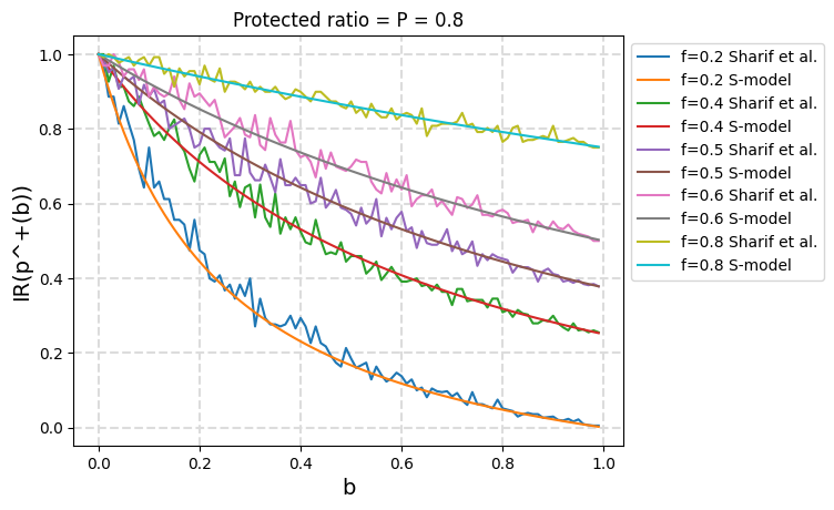
Figure 1: The S-model is the smoother version (expected value) of the randomized algorithm by (Žliobaitė 2017) - IR case, synthetic data.

Figure 2: The S-model is the smoother version (expected value) of the randomized algorithm by (Žliobaitė 2017) - 1/OR case, synthetic data.

(a) Adult dataset - IR

(b) Adult dataset - OR

Figure 3: Replica of Figure 5 from (Sharif and Baeza-Yates 2023) with the S-model.

Since we also model the case where $b<0$, we can use this extension to reproduce Figure 3 of (Žliobaitė 2017) (see Appendix C). In doing so, we found two inconsistencies: the OR curves are actually the elift ones and vice versa; and the IR curves actually correspond to $IR^{-1}$, i.e., inverting the roles of the protected and unprotected populations. Notice that IR is decreasing with positive bias addition since the numerator decreases and the denominator increases with $b$.

7 Formal Derivation of Our Measure

In this section we derive the Universal model (U-model), which stems from a more natural bias addition idea with stronger fundamental properties. We will later verify that the model actually computes $B_{U}(T)=b_{U}$.

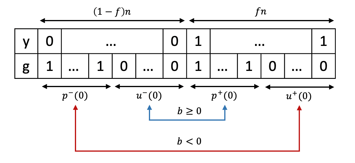
Figure 4: Illustrating the bias addition algorithm (U-model).

For the case when $b\geq 0$, this algorithm selects a fraction of size $|b|\cdot p^{+}(0)$ from the positive protected tuples and the same number of the negative unprotected tuples from the table. Labels from the selected tuples are then exchanged. When $b<0$ the same idea is used reverting the roles of $p$ and $u$. Namely, we instead take a fraction of $|b|\cdot u^{+}(0)$ pos. unprot. tuples, as well as the same quantity from the neg. prot. tuples $p^{-}(0)$ and exchange their labels. The process is illustrated in Figure 4. This results in an increase of the bias in favor of $p$, with an increase of $|b|\cdot u^{+}(0)$ in the set of pos. prot. tuples. Note that the $y^{+}$ invariant holds for this case as well. The pseudocode for the algorithm is given in Algorithm 1. In practice different tuple selections may cause different social impacts that have to be analyzed by domain experts. In this context, we restrict ourselves to the associated quantities. The induced transformation is derived in Theorem 7.1, together with the corresponding inversion that results in Theorem 7.2. Observe that the bias measure actually is $B_{U}(T)$ (Def. 4.1) when $C=1$.

0:  Bias parameter $b\in[-1,1]$; unbiased dataset $T_{0}$.

1:  if $b\not\in\mathcal{R}_{U}(b)$ then

2:     return  $\bot$

3:  else if $b\geq 0$ then

4:     Set $\delta_{b}=|b|\cdot p^{+}(0)$ 

5:     Select $\delta_{b}$ pos. prot. tuples, $\delta_{b}$ neg. unprot. tuples and exchange their labels

6:  else

7:     Set $\delta_{b}=|b|\cdot u^{+}(0)$ 

8:     Select $\delta_{b}$ pos. unprot. tuples, $\delta_{b}$ neg. prot. tuples and exchange their labels

9:  end if

Algorithm 1 U-model: bias addition algorithm.

Theorem 7.1 (Characterizing bias addition - U-model).

Given $b\in[-1,1]$, the transformation done by Algorithm 1 is given by

$$p^{+}(b)=\begin{cases}(1-b)\cdot p^{+}(0)&\quad\text{if $b\in[0,1]$}\\ (1-b)\cdot p^{+}(0)+by^{+}&\quad\text{if $b\in[-1,0)$}\\ \end{cases}$$ (1)

Theorem 7.2 (Inversion - U-model).

Inverting the relation given in Theorem 7.1 we get that for any dataset $T$, the required bias to get $p^{+}(b)$ per the U-model is given by

$$b=\begin{cases}1-\frac{p^{+}(b)}{p^{+}(0)}=1-\frac{f_{p(b)}}{f\cdot C}&\quad\text{if $b\in[0,1]$}\\ -1+\frac{y^{+}-p^{+}(b)}{y^{+}-p^{+}(0)}&\quad\text{if $b\in[-1,0)$}\\ \end{cases}$$

Note that the expression from Theorem 7.2 does not depend on $n$, which tells us that experimentally only one synthetic dataset is enough for computing the sought bias level. Also observe that one can implicitly know $\text{sg}(b)$ by noting $p^{+}(0)>p^{+}(b)\Leftrightarrow b>0$.

Bounds/valid range on the bias level

We observe that Algorithm 1 cannot always apply the desired bias value on the input table (cases when it outputs $\bot$). We provide the exact bounds for the range of valid $b$ values in Theorem 7.3, in terms of absolute table quantities.

Theorem 7.3 (Bounds on $b$ - U-model).

The added bias $b$ using the U-model satisfies

$$-1+\frac{y^{+}-\min(p,y^{+})}{y^{+}-p^{+}(0)}\leq b\leq 1-\frac{\max(0,y^{+}-(n-p))}{p^{+}(0)}$$

We denote this range by $\mathcal{R}_{U}(b)$, as shown in Table 1.

Based on the conditions of the problem, we provide the intuition behind the bounds in the Appendix (Section B).

8 Comparison with Other Bias Measures

In this section we compare our new bias measure to the standard ones and discuss its properties.

First, we note that the $elift$ measure (Pedreshi, Ruggieri, and Turini 2008) coincides with $1-b_{U}$ for $b_{U}$ as in Theorem 7.1 when exchanging the roles of $u$ and $p$. Second, later in Section 9, we show that:

$$p^{+}(b)=p^{+}(0)+|b|\cdot\Big{(}K^{\{U,S\}}_{\{+,-\}}-p^{+}(0)\Big{)}.$$

Then, recalling that every $\sigma\in\{IR,OR,elift,MD\}$ can be expressed as a function of $p^{+}(b)$, we can use function composition ($b\mapsto p^{+}(b)\mapsto\sigma(b)$) to get analytic expressions for every $\sigma$ solely in terms of $b$.

In fact, we can derive a compact expression for the $IR$ in terms of our new measure using simple algebraic manipulations:

Lemma 8.1.

Given a table $T$, $b=B_{U}(T)$ and $\hat{b}=\hat{B}_{U}(T)$ (Def. 8.1), we have

$$IR(b)=IR(T)=\begin{cases}\frac{1-b}{1+\hat{b}}&\quad\text{if the weak group is $P$}\\ \frac{1-\hat{b}}{1+b}&\quad\text{if the weak group is $U$}\\ \end{cases}$$

Given that $b$ and $\hat{b}$ have a natural and simple interpretation (as the fraction of positive entries of each group needed to recover the unbiased condition), one can use this result to argue that our new formal definition of bias is more suitable than the $IR$ as a measure of discrimination.

We now focus on comparing the properties of our measure $b_{U}$ against $IR$ and $MD$ as representatives for ratio and difference based measures, respectively. In Table 4 we already compare the values of these measures for three different types of tables.

Zero maps to unbiased

$b_{U}$ is the only ratio based measure that we are aware of whose unbiased value is $0$, which is the case for the difference based measures. This is beneficial, since it can be immediately mapped to the encoded notion of zero bias.

Duality - protected/unprotected

To the best of our knowledge, our measure is the first ratio based one that is dual w.r.t. the protected and unprotected groups: the magnitude of the difference w.r.t. the bias value has exactly the same semantics when switching the roles of these groups. Returning to the example from (Žliobaitė 2017), $IR=0.9$ and $IR=1.1$ represent a different amount of bias towards the protected ($IR<1$) and unprotected groups ($IR>1$), although both are at the same distance from the unbiased value $1$. This can also be seen in Table 4, where $T_{1}$ and $T_{2}$ are dual but where we have $IR=3/4$ and $IR=2$ respectively (and where $b_{U}$ has the same magnitude). Note that this is also the case for the $MD$, but this is because the measure considers additive biases (instead of multiplicative or ratio based ones, which is the case in our setting).

Duality - weak/strong

As noted before, when a dataset is biased there is a favored (strong) and a disadvantaged (weak) group w.r.t. equilibrium (i.e., the unbiased state). We can measure bias from the viewpoint of the weak group (as introduced before, denoted by $b$), but also from the perspective of the strong group, denoted by $\hat{b}$ which we call dual bias. Using the same ideas, one obtains Definition 8.1.

Definition 8.1.

Given a table $T$, its dual universal bias is given by

$$\hat{B}_{U}(T)=\hat{b}_{U}=\begin{cases}-1+\frac{f_{u(b)}}{f}&\quad\text{if $f_{p(b)}\leq f\leq f_{u(b)}$}\\ 1-\frac{f_{p(b)}}{f}&\quad\text{if $f_{u(b)}\leq f\leq f_{p(b)}$}\\ \end{cases}$$

Both $b$ and $\hat{b}$ model the problem under different perspectives and it is clear that these are not independent. In what follows we study their relation and explain its practical importance. Observe that when $f_{p(b)}\leq f\leq f_{u(b)}$, we have $b\geq 0$ and $\hat{b}\geq 0$. In this case, having bias $b$ means that there are $b\cdot p^{+}(0)$ less positive protected tuples w.r.t. equilibrium. In turn this means that the number of positive unprotected tuples exceeds equilibrium by this quantity as well. Thus, we have $\hat{b}\cdot u^{+}(0)=b\cdot p^{+}(0)\Leftrightarrow\hat{b}=b\cdot\frac{P}{U}$. Analogously, when $f_{u(b)}\leq f\leq f_{p(b)}$, it is the case that $b\leq 0$ and $\hat{b}\leq 0$. In the same vein, one gets $-b\cdot u^{+}(0)=-\hat{b}\cdot p^{+}(0)$. This equations make the relation between the $2$ dual biases explicit.

Looking at Table 4, for $T_{1}$ since $b_{U}=1/5$, $U=3/4$ and $P=1/4$ one has $\hat{b}_{U}=1/15$. For $T_{2}$, having $b_{U}=-1/5$ results in $\hat{b}_{U}=-3/5$. Note that in these cases a policy that completely eliminates bias would indeed have a drastically different impact for the stronger group depending on the case: Reaching equilibrium from $T_{1}$ causes a dual bias of magnitude $1/15$, while for the case of $T_{2}$ the magnitude is much higher ($3/5$). In our running example, this would mean that for $T_{2}$, $3/5$ of women (stronger group of $T_{2}$) would not get hired due to the mitigation policy. In light of this understanding enabled by our $2$ dual measures, the organization can now consider a more gradual implementation of the policy, perhaps designing a road-map to be implemented in a longer term. Thus, there are two complementary dualities in this problem:

1. When considering a given table, we can assess its bias level w.r.t. the weak group ($b$) or w.r.t. the strong group ($\hat{b}$). In this context the definitions are the same, but exchanging the roles of the strong and weak groups.

2. Additionally, we have the protected and unprotected groups and so, both when considering $b$ or $\hat{b}$, the bias for these two groups should have the same semantics. We encode this with the magnitude and sign of the biases.

Interpretability

As it was argued before, in a plethora of settings where bias has to be quantified one wants to capture the difference between proportions, as is the case with the unbiased condition stated before. Our measure captures this in an extremely easy way in the full range. In terms of the quantified bias, $|b_{U}|=k$ means that a $k\%$ the weakest group’s tuples need to change for the data to become unbiased (the sign indicates the group). This property holds for mitigation as well, as will be seen at the end of this section. For other measures, the interpretation of non-notable values (no discrimination, and maximum direct and reverse discrimination) is unclear. This is strongly undesirable, given that these are the most common in practice.

Computationally simple bias mitigation

From a computational perspective one can easily determine based on $b_{U}$ how the data needs to be transformed to become unbiased. In our example of Section 4, if one wants to transform a table with statistics $T_{1}$ into an unbiased version with statistics $T_{0}$, given that $b>0\Leftrightarrow p^{+}(b)<p^{+}(0)$, it suffices to implement policies such that the labels of $10=p^{+}(0)-p^{+}(b)$ neg. protected tuples are exchanged with positive unprotected ones. For $T_{2}$ (dual), since $b<0\Leftrightarrow p^{+}(b)>p^{+}(0)$ one needs to exchange the labels of $30$ positive protected tuples with neg. unprotected ones. We will discuss the details of bias mitigation in Section 10, including the need to incorporate domain experts into the process.

Based on the discussion above, we believe that our measure improves the state-of-the-art and thus we recommend to consider it when designing FairML pipelines to evaluate data bias.

9 Analyzing the Models

In this section we analyze the proposed models, discussing their similarities and significant differences. Particularly, in some regions of the parameter space $(P,f)$ their behavior coincide. We provide a complete characterization of the parameter space $(P,f)$ illustrating this in Figure 5. In what follows, when a parameter of an operator op (e.g., $\max$ or $\min$) is underlined, it means that when $\text{op}(\underline{1},2)=1$ then both models coincide.

Recall that for the S-model we have for $b\geq 0$, $p^{+}(b)=p^{+}(0)-b\min\big{(}\underline{p^{+}(0)},u^{-}(0)\big{)}$ and symmetrically for $b<0$. From these it follows (Theorem A.1) that $p^{+}(b)=$

$$\begin{cases}p^{+}(0)-b[p^{+}(0)-\max(\underline{0},y^{+}-(n-p))]&\text{if $b\geq 0$}\\ p^{+}(0)+b[p^{+}(0)-\min(\underline{y^{+}},p)]&\text{if $b<0$}\end{cases}$$

and thus, we get the unified form:

$$p^{+}(b) =p^{+}(0)+|b|\cdot\Big{(}K^{\{U,S\}}_{\{+,-\}}-p^{+}(0)\Big{)}$$

since $\text{sg}(b)\cdot b=|b|$ and where: $K^{S}_{+}=\max(0,y^{+}-(n-p))$, $K^{S}_{-}=\min(y^{+},p)$, $K^{U}_{+}=0$ and $K^{U}_{-}=y^{+}$. In particular, we can exactly characterize the regions of the parameter space where the models coincide. The different regions are shown in Figure 5. Based on this, the corresponding inversion result is

$$b={|p^{+}(b)-p^{+}(0)|}/{\big{(}p^{+}(0)-K^{\{U,S\}}_{\{+,-\}}\big{)}}$$ (2)

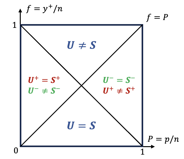
Figure 5: Parameter space with model differences.

Using the unified form and recalling that $\vec{b}$ is the value such that $p_{s}^{+}(\vec{b})=p_{r}^{+}(0)$, we immediately get the unified expression for it:

$$\vec{b}=|p_{r}^{+}(0)-p_{s}^{+}(0)|/\big{(}p_{s}^{+}(0)-K^{\{U,S\}}_{\{+,-\}}\big{)}$$ (3)

Bias saturation

One of the key differences between both models is that the S-model always adds bias to the input table (in a non-uniform way). Does this always make sense in practice? Consider the following example: Suppose we are analyzing data where $C=1$, $n=1000$, $P=0.4$ and $f=0.8$. In this setting we initially have (for $b=0$): $p^{+}(0)=320$ and $u^{+}(0)=480$. If we want to add $b=1$, which conceptually means “assign all protected members $y=0$”, $320$ positive protected tuples should be changed. Due to the $y^{+}$ invariance, $320$ negative unprotected tuples should change as well, which is not possible since $u^{-}(0)=120$. The upper bound for this example is $b=1-\frac{p^{+}(b)}{p^{+}(0)}=\frac{3}{8}$, which coincides with Theorem 7.3. It suffices for $P>1-f$ in order to have $b<1$. Additionally, if $P+f\leq 1$, $b=1$ can be reached. Thus, in half of the cases this is not possible, which shows this happens for a non-negligible set of instances.

Bias intervals resulting in the same table

As shown at the beginning of this section, given a table we may conclude using Equation 2 that its bias level is a single value $\bar{b}$. However, since $p^{+}(0)$ is an integral quantity, we observe that there is a range of $b$ values for which, when starting with $p^{+}(0)$ positive protected tuples, one ends up with $p^{+}(b)$ such tuples in the output table. We explicitly find this interval next and suggest the value that should be chosen from it in practice. To the best of our knowledge, previous work does not consider such intervals, which can be relevant for practical applications (e.g., fair ML).

Using the unified definition of $p^{+}(b)$ and adding an arbitrary increment $\delta\in\mathbb{R}$ we get:

$$p^{+}(b)+\delta =p^{+}(0)+|b|\Big{(}K^{\{U,S\}}_{\{+,-\}}-p^{+}(0)\Big{)}+\delta$$

$$=p^{+}(0)+b^{*}\Big{(}K^{\{U,S\}}_{\{+,-\}}-p^{+}(0)\Big{)}$$

Thus if we want to get $p^{+}(b)+\delta$ pos. prot. tuples it suffices to use $b^{*}$ as the bias level. Given that $\bar{b}$ is the exact bias level we compute, we suggest taking the closest integer to $p^{+}(\bar{b})$, $\lfloor p^{+}(\bar{b})\rceil\in\mathbb{N}$. Recalling that $\lfloor x\rceil:=\lfloor x+0.5\rfloor$, we get

$$\lfloor p^{+}(b)+\delta\rceil=\lfloor p^{+}(b)+\delta+0.5\rfloor=p^{+}(b)\Leftrightarrow-0.5\leq\delta<0.5$$

Noting that $\text{sg}(b)\cdot\Big{(}K^{\{U,S\}}_{\{+,-\}}-p^{+}(0)\Big{)}=-\Big{|}K^{\{U,S\}}_{\{+,-\}}-p^{+}(0)\Big{|}$, we conclude that the set is given by

$$\mathcal{R}=\Big{[}\bar{b}-\frac{0.5}{\Big{|}K^{\{U,S\}}_{\{+,-\}}-p^{+}(0)\Big{|}},\bar{b}+\frac{0.5}{\Big{|}K^{\{U,S\}}_{\{+,-\}}-p^{+}(0)\Big{|}}\Big{)}.$$

Uniformity

The key property that differentiates the U-model with respect to the S-model is its uniformity: in order to transition from a bias value of $b_{1}$ to $b_{2}$, the number of label inversions that are done by the model increases proportionally (linearity is another desired property for a bias measure). In particular, the number of inversions are independent from the table’s parameters (see Table 5). On the contrary for the S-model, the bias values depend on the parameters and are not uniform. Understanding how these parameters influence the output of the model is non-trivial and outside the scope of a data analyst or policy maker working with the model. This results in the outputs of the S-model being way harder to interpret in practice. This fact can also be analytically studied to precisely quantify the difference, as we do next. As explained at the beginning of this section, if $u^{-}(0)\geq p^{+}(0)$ the S and U models coincide. However, if $u^{-}(0)<p^{+}(0)$, for every $b>0$ only a fraction $\frac{bu^{-}(0)}{bp^{+}(0)}$ of the $bp^{+}(0)$ pos. prot. tuples are exchanged under the S-model. We say that the U-model, is uniform in the sense that when it does not fail, it always exchanges the labels of $bp^{+}(0)$ pos. prot. tuples. In particular, when the models differ we have $b_{U}=b_{S}\cdot\frac{u^{-}(0)}{p^{+}(0)}$. We will revisit this phenomena considering real datasets in Section 10, where the data will be analyzed in the context of bias mitigation.

$n$	$y^{+}$	$p$	$p^{+}(0)$	$b_{S}$	$b_{U}$	$b_{S}/b_{U}=$
						$p^{+}(0)/u^{-}(0)$
2700	900	1800	600	0.10	0.10	1
2400	900	1600	600	0.12	0.10	1.2
1800	900	1200	600	0.20	0.10	2.0
1440	900	960	600	0.33	0.10	3.3
1200	900	800	600	0.60	0.10	6.0
1140	900	760	600	0.75	0.10	7.5
960	900	640	600	1.00	0.10	10

Table 5: U-model is uniform, while the S-model depends on the table values.

10 Bias Mitigation in Practice

As explained in Section 5, when considering a bias mitigation strategy (fundamental practical application of interest) we want a procedure to convert a real (potentially biased) table into an “ideal” unbiased one. Our framework can be applied in this way as well, simply by reverting the roles of the input and output tables (i.e., using the real table as input). The associated bias value is what we call backward bias, while the other one is called forward bias. We provide both bias values for each dataset in Table 6. We will analyze these values to further elaborate the observations made with respect to the uniformity of the models.

Name	$p_{s}^{+}(b)$	$p_{s}^{+}(0)=$	S-f	U-f	S-b	U-b
		$\lfloor y^{+}p/n\rceil$
Abalone	883	651	-0.35	-0.16	0.26	0.26
Adult	1179	2594	0.55	0.55	-0.21	-0.21
Autism	103	90	-0.13	-0.13	0.13	0.13
Bank	2755	3184	0.13	0.13	-0.17	-0.17
Compas	11552	8595	-0.27	-0.27	0.26	0.26
Default	3763	4006	0.06	0.06	-0.08	-0.08
Diabetes	153	143	-0.11	-0.06	0.08	0.07
Fertility	10	10	0	0	0	0
Kidney	212	193	-0.33	-0.33	0.36	0.09

Table 6: Real datasets - forward and backward bias values for both models.

Note for example that the Kidney dataset exhibits the same forward values (S-f$=$U-f), but for the S-model four times more bias is required in the opposite direction (S-b$=4\cdot$U-b). Additionally, consider what happens with the Diabetes and Autism datasets: although their forward values are close under the S-model (i.e., $-0.11\approx-0.13$), the corresponding forward value under the U-model for Autism ($-0.13$) is almost double the one for Diabetes ($-0.06$), i.e., we have found two real datasets with practically equal S-f values but significantly different U-f values. Thus, it is also the case in practice that when looking at the bias values from the S-model in an absolute manner (without taking other table parameters into account) one gets confusing information about the underlying process. As we saw in Section 4, the interpretation using the U-model is simple: a fraction of $b\cdot x$ protected tuples were exchanged to get to the output table.

In light of this perspective, from a computational point of view the solution to achieve an unbiased table is now straightforward: Let $\delta:=|p_{r}^{+}(0)-p_{s}^{+}(0)|$. Then, if $p_{r}^{+}(0)>p_{s}^{+}(0)$ one needs to exchange the labels of $\delta$ positive protected tuples from the table and if $p_{r}^{+}(0)<p_{s}^{+}(0)$ one should perform the exchange with $\delta$ negative protected tuples; both cases until reaching the target unbiased quantity $p_{s}^{+}(0)$. What is not simple though, is to know how to promote societal policies to attain this objective. Policy makers and domain experts are needed in conjunction with our results to implement effective bias mitigation strategies.

11 Conclusions and Future Work

In this section we present additional conclusions of our work and future extensions.

Easy interpretation

Normally since neither an institution’s management nor their data analysts have a highly specialized statistical knowledge, it is strongly desirable to have a bias measure satisfying the properties mentioned in Section 8, most crucially one that is both easy to compute and interpret, to quantify the bias in the data. Additionally, given that the fundamental practical objective is the mitigation of the bias, one would also like the bias measure to give insights into this process as well. Our new bias measure achieves this.

No need to “go beyond” table quantities

For both models, but in particular for the bias addition algorithm from the S-model it suffices to study the changes of $p^{+}(b)$ to derive/measure a bias value. In particular, there is no need as done in previous work, most notably (Žliobaitė 2017; Sharif and Baeza-Yates 2023), to use any estimator depending on $p^{+}(b)$. Our approach provides a mathematically rigorous way to quantify $p_{s}^{+}(b)$ (and if we can invert the relation, to obtain $b$), but also since we know the target “ideal situation” $p_{s}^{+}(0)$ and what actions to take (namely invert $|p_{r}^{+}(0)-p_{s}^{+}(b)|$ labels from the corresponding tuples) we can provide a bias mitigation technique, which is ultimately the end goal in the case of harmful bias. This mitigation strategy, together with our new measure are two of the main practical contributions of our paper.

Dynamic assessment of policies

Once a bias is detected in the context of an institutional process, a different policy for future decisions may want to be implemented. This new policy will cause the data to change (removing or adding new tuples from/to the table) which means that the new bias will have to be recomputed dynamically to assess the new policy. One can trivially recompute our measure to monitor this evolution at the desired time granularity automatically. This is also the case for the $IR$, $OR$, $elift$ and $MD$, but the key difference is that with our measure, every time it is recomputed there is a simple and clear interpretation, regardless of the value: the new value of $b_{U}$ is the proportion of positive elements from the weakest group that needs to be added to get to the unbiased state.

Flexibility of our approach

Besides the two models presented in this work, our framework is flexible in the sense that one may change the bias concept and when analyzing it, one can derive a new model. In essence, if one can provide an “algorithmic explanation” of the bias idea (quantified and inverted) one can derive a new bias model. This is significant as, a priori, bias notions are relatively arbitrary and it is important for a framework with the end objective of measuring this concept, to incorporate this requirement.

Dynamic evaluation

The use of our measure can be extended in a natural way to assess the dynamic evaluation of the data, which includes the case of up or down-sampling, where tuples are added or deleted. In this setting, one can simply recompute our measure several times during the data evaluation, thus assessing how the changes (which in practice may be the result of applying mid and long term institutional policies) affect the bias of the data.

Non binary case and other extensions

A straightforward extension to the multi-attribute sensitive setting consist of selecting a subset of the attributes to define the protected group $\mathcal{P}=\{t:t[a_{1}]=c_{1,i}\wedge\dots\wedge t[a_{n}]=c_{n,k}\}$ and setting the rest of the tuples to be the unprotected group $\mathcal{U}=T\setminus\mathcal{P}$. We can also extend the measures to consider randomized updates or dependencies between different entries of the table.

Applications to data discovery

In the context of Responsible Data Management, one can envision data discovery algorithms that incorporate our measure as part of their objectives. This can help to incorporate robustness, fairness, interpretability and legal compliance into existing data-driven algorithmic systems.

12 Acknowledgments

The authors would like to thank Renée Miller for the insightful discussions and suggestions for improving earlier versions of this work.

Appendix A S-Model, omitted details

We present an equivalent simpler version of the bias addition algorithm from (Žliobaitė 2017) for $b\in[-1,1]$ in Algorithm 2. Depending on $\text{sg}(b)$ the algorithm starts by deterministically creating a sub-table with $bp^{+}(0)$ positive protected tuples and $bu^{-}(0)$ negative unprotected tuples (when $b\geq 0$) or one with with $bp^{-}(0)$ negative protected tuples and $bu^{+}(0)$ positive unprotected tuples (when $b<0$). We use the subscript st to refer to the quantities of this sub-table.

Then, for the case when $b\in[0,1]$, we take a tuple with $g=0\wedge y=0$ and one with $g=1\wedge y=1$ (blue arrow) and invert their labels. For $b\in[-1,0)$ the same is done symmetrically considering a pair of tuples with $g=1\wedge y=0$ and $g=0\wedge y=1$ (red arrow). We repeat this process $\Delta p_{st}^{+}(b)$ times, given by the minimum size of the two groups we are considering (see Figure 6). We note that the algorithm maintains $y^{+}$ invariant, as required by our framework.

Note that our aim is to quantify the variation of $p^{+}(b)$ as a function of $b$ (as will be done in Theorem A.1 for this model). For clarity we present the underlying table transformation in the algorithm, but when implementing it, it suffices to operate directly with the equations and the quantities of interest (i.e., table transformations can be avoided). In particular, it is not relevant to individually identify the tuples being selected. In practice this could be of crucial social interest and thus has to be assessed by domain experts.

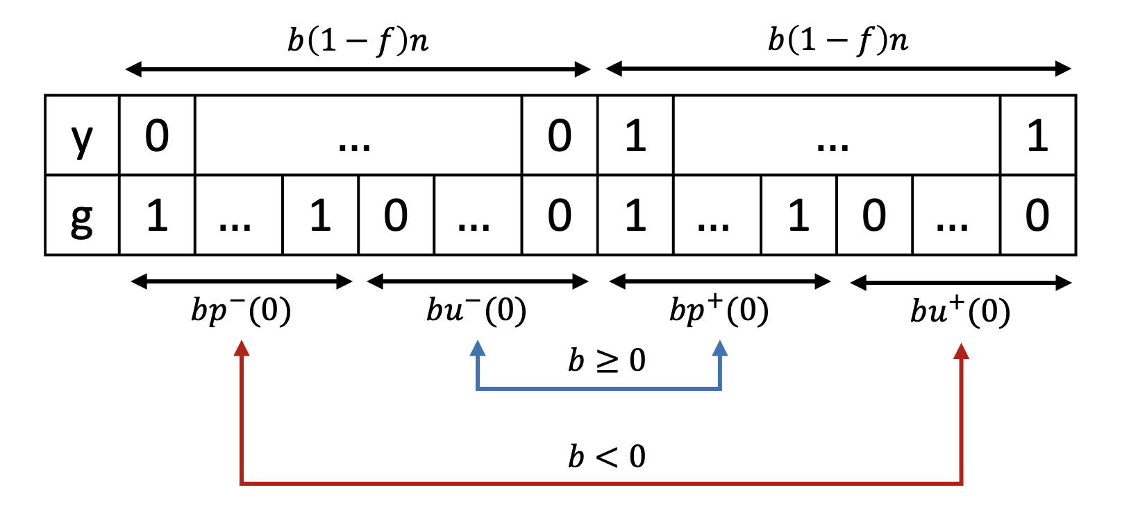
Figure 6: Diagram illustrating the bias addition algorithm of the S-model for $b\in[-1,1]$.

0:  Bias parameter $b\in[-1,1]$; unbiased dataset $T_{0}$.

1:  Compute $y^{+}$, $n$ and $p$ 

2:  if $b\geq 0$ then

3:     Create a subtable with $|b|p^{+}(0)$ pos. prot. tuples and $|b|u^{-}(0)$ neg. unprot. tuples 

4:     Select from the subtable: $\Delta p_{st}^{+}(b)$ pos. prot. tuples, $\Delta p_{st}^{+}(b)$ neg. unprot. tuples and exchange their labels 

5:  else

6:     Create a subtable with $|b|p^{-}(0)$ neg. prot. tuples and $|b|u^{+}(0)$ pos. unprot. tuples 

7:     Select from the subtable: $\Delta p_{st}^{+}(b)$ neg. prot. tuples, $\Delta p_{st}^{+}(b)$ pos. unprot. tuples and exchange their labels 

8:  end if

9:  return  modified table

Algorithm 2 S-model: bias addition algorithm.

We derive the induced transformation explicitly in Theorem A.1, presenting a single equation for the full range $b\in[-1,1]$. Based on this result, we invert the relation obtaining Theorem A.2, which provides the exact bias value to obtain a desired number of positive protected tuples in the modified table. The proofs of these theorems are given in Appendix B.

Theorem A.1 (Characterizing bias addition - S-model).

Given $b\in[-1,1]$, the transformation done by Algorithm 2 is given by

$$p^{+}(b)=\begin{cases}p^{+}(0)-b[p^{+}(0)-\max(0,y^{+}-(n-p))]&\text{if $b\geq 0$}\\ p^{+}(0)+b[p^{+}(0)-\min(y^{+},p)]&\text{if $b<0$}\end{cases}$$

Theorem A.2 (Inversion - S-model).

Inverting the relation given in Theorem A.1 we get that for any dataset $T$, the required bias to get $p^{+}(b)$ per the S-model is given by

$$b=\begin{cases}\frac{p^{+}(0)-p^{+}(b)}{p^{+}(0)-\max(0,y^{+}-(n-p))}&\quad\text{if $b\geq 0$}\\ -\frac{p^{+}(0)-p^{+}(b)}{p^{+}(0)-\min(y^{+},p)}&\quad\text{if $b<0$}\end{cases}$$

Valid Range for the Bias

The S-model admits the full range of possible $b$ values, i.e., $[-1,1]$.

Appendix B Omitted Proofs

Proof of Theorem A.1

Proof.

First we note that

$$p^{+}(b)=\begin{cases}p^{+}(0)-b\min(p^{+}(0),u^{-}(0))&\quad\text{if $b\geq 0$}\\ u^{+}(0)+b\min(p^{-}(0),u^{+}(0))&\quad\text{if $b<0$}\end{cases}$$

where $u^{-}(0)=u-u^{+}(0)=(n-p)-(y^{+}-p^{+}(0))$.

Thus,

$$\min(p^{+}(0),u^{-}(0))=p^{+}(0)-\max(0,y^{+}-(n-p)).$$

Analogously, since $u^{+}(0)=y^{+}-p^{+}(0)$ and $p^{-}(0)=p-p^{+}(0)$, then

$$\min(p^{-}(0),u^{+}(0))=-p^{+}(0)+\min(y^{+},p)$$

Using these, the result follows that $p^{+}(b)=$

$$\begin{cases}p^{+}(0)-b[p^{+}(0)-\max(0,y^{+}-(n-p))]&~{}\text{if $b\geq 0$}\\ p^{+}(0)+b[p^{+}(0)-\min(y^{+},p)]&~{}\text{if $b<0$}\end{cases}$$

∎

Proof of Theorem 7.1

Proof.

For $b>0$ the result clearly follows. For $b<0$, note that we have $u^{+}(b)=(1-b)\cdot u^{+}(0)$ and by noting that $u^{+}(b)=y^{+}-p^{+}(b)$ (and $u^{+}(0)=y^{+}-p^{(}0)$) we get the result. ∎

Proof of Theorem 7.3

Proof.

The result follows from Theorem 7.2 and by the fact that $\max(0,y^{+}-(n-p))\leq p^{+}(b)\leq\min(p,y^{+})$. ∎

Intuition Behind the Bounds

In what follows, we provide the intuitions behind the bounds found in Theorem 7.3. Note that for $b>0$ when $b\rightarrow 1$, $p^{+}(b)\rightarrow 0$ and conversely for $b<0$ when $b\rightarrow-1$, $u^{+}(b)\rightarrow 0$.

If $p^{+}(b)=0$ this means that $u^{+}(b)=y^{+}$. But note that if $y^{+}>(n-p)=u\geq u^{+}(b)$, then $u^{+}(b)<y^{+}$ and thus $p^{+}(b)$ can never reach 0. Analogously, if $u^{+}(b)=0$ we must have $p^{+}(b)=y^{+}$, but if $y^{+}>p$ this cannot be the case.

Appendix C S-model Validation

Figure 3 of (Žliobaitė 2017) is reproduced using the S-model, shown in Figure 7.

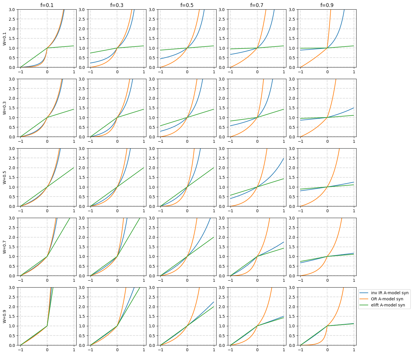
Figure 7: Replica of Figure 3 of (Žliobaitė 2017) using the S-model.

References

- Angwin et al. (2016) Angwin, J.; Larson, J.; Mattu, S.; and Kirchner, L. 2016. How We Analyzed the COMPAS Recidivism Algorithm.
- Baeza-Yates (2018) Baeza-Yates, R. 2018. Bias on the Web. Commun. ACM, 61(6): 54–61.
- Becker and Kohavi (1996) Becker, B.; and Kohavi, R. 1996. Adult. UCI Machine Learning Repository. DOI: https://doi.org/10.24432/C5XW20.
- Calders and Žliobaitė (2013) Calders, T.; and Žliobaitė, I. 2013. Why Unbiased Computational Processes Can Lead to Discriminative Decision Procedures. In Custers, B.; Calders, T.; Schermer, B.; and Zarsky, T., eds., Discrimination and Privacy in the Information Society: Data Mining and Profiling in Large Databases, 43–57. Berlin, Heidelberg: Springer Berlin Heidelberg. ISBN 978-3-642-30487-3.
- Calmon et al. (2017) Calmon, F.; Wei, D.; Vinzamuri, B.; Natesan Ramamurthy, K.; and Varshney, K. R. 2017. Optimized Pre-Processing for Discrimination Prevention. In Guyon, I.; Luxburg, U. V.; Bengio, S.; Wallach, H.; Fergus, R.; Vishwanathan, S.; and Garnett, R., eds., Advances in Neural Information Processing Systems, volume 30. Curran Associates, Inc.
- Gastwirth (2021) Gastwirth, J. L. 2021. A Summary of the Statistical Aspects of the Procedures for Resolving Potential Employment Discrimination Recently Issued by the Office of Federal Contract Compliance Along with a Commentary. SSRN.
- Gil and Girela (2013) Gil, D.; and Girela, J. 2013. Fertility. UCI Machine Learning Repository. DOI: https://doi.org/10.24432/C5Z01Z.
- Hort et al. (2023) Hort, M.; Chen, Z.; Zhang, J. M.; Harman, M.; and Sarro, F. 2023. Bias Mitigation for Machine Learning Classifiers: A Comprehensive Survey. ACM J. Responsib. Comput. Just Accepted.
- Jang, Zheng, and Wang (2021) Jang, T.; Zheng, F.; and Wang, X. 2021. Constructing a Fair Classifier with Generated Fair Data. Proceedings of the AAAI Conference on Artificial Intelligence, 35(9): 7908–7916.
- Kanagarathinam (2020) Kanagarathinam, K. 2020. Early stage diabetes risk prediction. UCI Machine Learning Repository. DOI: https://doi.org/10.24432/C5VG8H.
- Mehrabi et al. (2021) Mehrabi, N.; Morstatter, F.; Saxena, N.; Lerman, K.; and Galstyan, A. 2021. A survey on bias and fairness in machine learning. ACM computing surveys (CSUR), 54(6): 1–35.
- Moro, Rita, and Cortez (2012) Moro, S.; Rita, P.; and Cortez, P. 2012. Bank Marketing. UCI Machine Learning Repository. DOI: https://doi.org/10.24432/C5K306.
- Nash et al. (1995) Nash, W.; Sellers, T.; Talbot, S.; Cawthorn, A.; and Ford, W. 1995. Abalone. UCI Machine Learning Repository. DOI: https://doi.org/10.24432/C55C7W.
- Olteanu et al. (2019) Olteanu, A.; Castillo, C.; Diaz, F.; and Kıcıman, E. 2019. Social data: Biases, methodological pitfalls, and ethical boundaries. Frontiers in big data, 2: 13.
- Osoba et al. (2024) Osoba, O. O.; Badrinarayanan, S.; Cheng, M.; Rogers, R.; Jain, S.; Tandra, R.; and Pillai, N. 2024. Responsible AI update: Testing how we measure bias in the U.S.
- Pedreshi, Ruggieri, and Turini (2008) Pedreshi, D.; Ruggieri, S.; and Turini, F. 2008. Discrimination-aware data mining. In Proceedings of the 14th ACM SIGKDD International Conference on Knowledge Discovery and Data Mining, KDD ’08, 560–568. New York, NY, USA: Association for Computing Machinery. ISBN 9781605581934.
- Rubini, Soundarapandian, and Eswaran (2015) Rubini, L.; Soundarapandian, P.; and Eswaran, P. 2015. Chronic Kidney Disease. UCI Machine Learning Repository. DOI: https://doi.org/10.24432/C5G020.
- Sharif and Baeza-Yates (2023) Sharif, A.; and Baeza-Yates, R. 2023. Measuring Bias. In 2023 IEEE International Conference on Big Data (Big Data). Sorrento, Italy: IEEE CS Press.
- Suresh and Guttag (2021) Suresh, H.; and Guttag, J. 2021. A framework for understanding sources of harm throughout the machine learning life cycle. In First ACM Conference on Equity and access in algorithms, mechanisms, and optimization, 1–9. Stanford, CA, USA: ACM Press.
- Thabtah (2017) Thabtah, F. 2017. Autism Screening Adult. UCI Machine Learning Repository. DOI: https://doi.org/10.24432/C5F019.
- Yeh (2016) Yeh, I.-C. 2016. Default of credit card clients. UCI Machine Learning Repository. DOI: https://doi.org/10.24432/C55S3H.
- Žliobaitė (2017) Žliobaitė, I. 2017. Measuring discrimination in algorithmic decision making. Data Mining and Knowledge Discovery, 31(4): 1060–1089.