Theory of fractional quantum Hall liquids coupled to quantum light and emergent graviton-polaritons

Abstract

Recent breakthrough experiments have demonstrated how it is now possible to explore the dynamics of quantum Hall states interacting with quantum electromagnetic cavity fields. While the impact of strongly coupled non-local cavity modes on integer quantum Hall physics has been recently addressed, the effects on fractional quantum Hall (FQH) liquids – and, more generally, fractionalized states of matter – remain largely unexplored. In this work, we develop a theoretical framework for the understanding of FQH states coupled to quantum light. In particular, combining analytical arguments with tensor network simulations, we study the dynamics of a $\nu=1/3$ Laughlin state in a single-mode cavity with finite electric field gradients. We find that the topological signatures of the FQH state remain robust against the non-local cavity vacuum fluctuations, as indicated by the endurance of the quantized Hall resistivity. The entanglement spectra, however, carry direct fingerprints of light-matter entanglement and topology, revealing peculiar polaritonic replicas of the $U(1)$ counting. As a further response to cavity fluctuations, we also find a squeezed FQH geometry, encoded in long-wavelength correlations. We additionally observe that moving to strong cavity field gradients leads to an instability towards a sliding Tomonaga-Luttinger liquid phase, featuring a strong density modulation in the gradient direction. Finally, by exploring the low-energy excited spectrum inside the FQH phase, we identify a new quasiparticle, the graviton-polariton, arising from the hybridization between quadrupolar FQH collective excitations (known as gravitons) and light. We discuss the experimental implications of our findings and possible extension of our results to more complex scenarios.

I Introduction

The possibility of controlling quantum matter properties via cavity embedding has sparked a lot of interest in recent years [1, 2, 3, 4]. Vacuum fluctuations of strongly confined electromagnetic modes have been proposed as handles on various phenomena [5, 6, 7, 8, 9, 10, 11, 12, 13, 14, 15], and pioneering experiments have demonstrated the non-trivial role of cavity quantum electrodynamics (QED) set-ups in shaping matter properties [16, 17, 18, 19, 20]. A particularly intriguing framework is that of topological phases, whose traditional many-body understanding faces fundamentally new questions due to the non-local nature of the cavity degree of freedom.

On this point, a recent breakthrough experiment  [16] has shown that the Hall conductivity of the integer quantum Hall (IQH) effect can be affected by a split-ring cavity in the ultra-strong coupling regime, even in the absence of any driving. This effect has been proposed to arise from cavity mediated hoppings [21] involving cyclotron transitions to higher Landau levels (LLs) assisted by vacuum photons or, more recently, as a consequence of cavity losses [22]. Although a rather good understanding of IQH states coupled to quantum light has been developed, its effect on the much richer physics of fractional quantum Hall (FQH) matter [23, 24] remains largely unexplored.

The FQH effect [23] is a fundamentally different state of matter which, differently from its integer counterpart, genuinely arise from many-body correlations. In FQH phases, new collective degrees of freedom emerge, such as anyonic quasi-particles [25], one of the smoking gun of topological order, or magnetoroton modes [26, 27] also dubbed at long wavelength as gravitons [28] given the link to a more recent geometric description of FQH correlations [29, 30, 31, 32]. Another unique feature of topologically ordered phases is their peculiar many-body entanglement structure [33, 34], which naturally connects to spectral properties and has been demonstrated an useful tool for the classification of quantum phases of matter. What is the fate of such rich and profound phenomena under the action of quantum light? This is the question we address in this work.

We put forward a theory describing FQH liquids coupled to quantum light. The starting point of our analysis is a careful modeling of electrons coupled to light, that preserves a restricted gauge invariance exactly. We introduce a lowest Landau level (LLL) projected minimal coupling, following Ref. [35], which neglects cyclotron transitions and focuses on intra-LL physics. This highlights the role of cavity field gradients which, in agreement with Kohn’s theorem [36], are essential to non-trivially couple to electronic correlations within the LLL.

As a proof of principle, we investigate a simplified scenario given by the $\nu=1/3$ Laughlin state coupled to a cavity with a constant gradient, and no losses. The setting is schematically depicted in Fig. 1. The full quantum dynamics of the system (light and matter) is studied numerically with a novel hybrid tensor network ansatz that combines the success in representing FQH states [38, 39] using matrix product states (MPS) [40, 41, 42], with cavity-matter correlations in 1D [43, 44, 45, 46]. This allows us to investigate in an unbiased manner both ground and excited states properties, using algorithms based on the density-matrix-renormalization group (DMRG) [47, 48] and on the time-dependent variational principle (TDVP) [49, 50].

We show that the topological properties of the Laughlin state remain stable against the introduction of the non-local mode, as signaled by the quantized Hall resistivity, which we calculate by adapting the original flux insertion argument [51]. However, entanglement properties are drastically affected: new entanglement spectrum features arise in form of copies of the typical $U(1)$ counting of FQH states [33], which appear separated by a polariton entanglement gap. This reveals a collective coupling with matter excitations at zero transferred momenta which we also detect in spectral properties. These matter excitations are revealed to be gravitons, i.e., the long-wavelength part of the magnetoroton dispersion, and, once they hybridize with cavity photons, become graviton-polaritons. They give rise to a typical polariton doublet, which can be used in spectroscopy experiments as a smoking gun for the strong-coupling regime. Through a simple effective model that almost matches quantitatively with the finite size numerical simulations, we also provide analytical predictions for the collective Rabi frequency in terms of the known graviton quadrupole moment.

Another major consequence of the cavity mode on the ground state is the squeezing of the FQH metric [29], that is revealed by a striking change in long-wavelength correlations and by the spatially anisotropic profile of electron correlation holes. Inspecting field gradients which are strong at the single particle level, we also find a cavity mediated instability accompanied by the softening of the full magnetoroton dispersion. The strong coupling phase has strong density modulations organized as stripes which can be understood as a sliding Tomonaga-Luttinger liquid phase, reminiscent of other transitions mediated by different anisotropy sources [52].

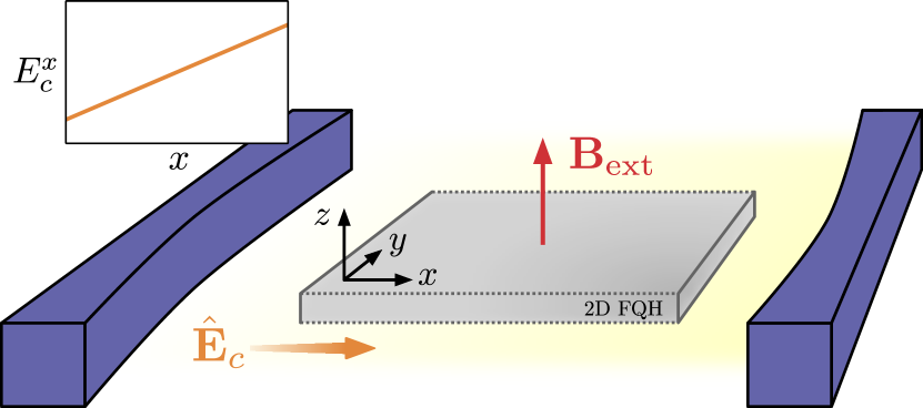
Figure 1: Illustration of the FQH bar placed inside the cavity. The electrons are confined to move in the 2D plane under the action of a perpendicular magnetic field $\bm{B}_{\mathrm{ext}}$. The in-plane component of the cavity electric field pierces the principal edges of the strip perpendicularly. Periodic boundary conditions on $y$ are depicted as dotted edges, while open boundary conditions on $x$ are depicted as a sharp cut. The inset shows the mode profile with a uniform gradient used in most of the discussion.

Summary of results.—

Before describing the structure of the work, we summarize here our main findings:

• A microscopic QED theory describing the coupling of quantum light to electrons in the LLL, pointing out that constant fields have no effects on the latter;

• Resilience of quantized Hall resistivity upon the introduction of the non-local cavity-mode degree of freedom, with the latter imprinting an anisotropic FQH geometry in the ground state;

• A new entanglement structure in hybrid quantum Hall states, where the role of quantum light is to introduce a “band” of chiral Luttinger liquids multiplets, each with an approximately quantized photon number;

• The prediction of graviton-polariton modes, describing the hybridization of the typical magnetoroton mode with quantum light in the setup we consider;

• The prediction of an instability of Laughlin states to sliding Luttinger liquids at a very strong light-matter coupling for cavities describing constant electric field gradients.

The paper is organized as follows.

In Section II we describe the system under study, starting from a brief recap on LLs and the microscopic derivation of the light-matter coupling by means of a minimal substitution restricted to the LLL, ensuring gauge invariance and a proper treatment of the strong coupling regime. We discuss the role of cavity field gradients, and detail the numerical methods we use to solve the full cavity-matter problem.

In Section III we present a detailed study of the nature of the FQH topological order in the presence of a strongly coupled non-local cavity degree of freedom. We do so by looking at two key markers, the entanglement spectrum structure and the transverse Hall resistivity. We also provide numerical evidence that cavity vacuum fluctuations lead to a squeezed FQH geometry.

In Section IV, we discuss the phase diagram and the instability to a sliding Tomonaga-Luttinger liquid phase in the regime of strong field-gradients at the single electron level. We first present finite size numerical results, and then motivate the existence of an instability on the basis of a photon mean-field decoupling. We present a qualitative field theory describing the sliding Tomonaga-Luttinger liquids, where light-matter correlations can be reintroduced to some extent.

In Section V we investigate bulk spectral properties of the hybrid light-matter FQH state. We start by reviewing the magnetoroton spectrum, the low energy gapped neutral excitations on top of FQH states. Then we present numerical evidence for the effect of the cavity degree of freedom on the full magnetoroton dispersion, from the formation of the hybrid graviton-polariton to the lowering of the magnetoroton minimum as precursor of the instability. We then construct an effective model which builds on top of the Girvin-MacDonald-Platzman (GMP) treatment of magnetorotons, and is able to capture analytically the salient features of the graviton-polaritons that we observe numerically.

In Section VI, we discuss the connection of our findings to realistic experimental scenarios taking as a reference a split-ring resonator [16]. While energy scales match, we highlight how carefully designed resonators with strong field gradients are needed to reach strong coupling to FQH physics. We also comment on the possible role of cavity screening of Coulomb interactions neglected in our treatment.

To conclude in Section VII, we summarize our results and draw a more general picture on how confined electromagnetic modes can be used to both probe and control correlations in the LLL.

II The model

In this section we start by reviewing LL physics (Sec. II.1) and the split-ring cavity set-up (Sec. II.2). Then, we present the first result of this work, namely the derivation of a QED Hamiltonian for LLL electrons coupled to a cavity (Sec. II.3). After discussing some of the physical implications of the obtained model (Sec. II.4), we spell out the full Hamiltonian used in the rest of the paper (Sec. II.5) and describe the MPS ansatz used to solve it (Sec. II.6).

II.1 Landau Levels

We consider a collection of $N_{e}$ electrons with mass $m_{e}$ and elementary charge $q=|e|$ living on the $(x,y)$ plane under a strong magnetic field $\bm{B}_{\mathrm{ext}}=(0,0,B)$ in the $z$-direction (Fig. 1), represented in the so called Landau gauge by an external vector potential $\bm{A}_{\mathrm{ext}}=(0,xB,0)$. We choose to work with periodic boundary conditions along $y$, implying a cylinder geometry with a finite circumference $L_{y}$. The single-particle eigenstates can be written as [53]:

$$\psi_{n,k}(x,y)=\frac{1}{\sqrt{L_{y}}}e^{iky}\phi_{n}(x-X_{k}),\qquad k=\frac{2\pi}{L_{y}}j_{k},$$ (1)

with $n=0,1,2,...,$ being the LL index and $j_{k}\in\mathbb{Z}$ labeling the momentum along $y$. Here $\phi_{n}$ are eigenfunctions of the harmonic oscillator with characteristic length equal to the magnetic length $l_{B}=\sqrt{\frac{\hbar c}{eB}}$, frequency equal to the cyclotron frequency $\omega_{B}=\frac{eB}{m_{e}}$, and centered around $X_{k}=kl_{B}^{2}$. In presence of an external potential $W$, which can account for both disorder and confining potential, the single-particle Hamiltonian for the LLs takes the following general form:

$$\hat{\mathcal{H}}_{0}=\sum_{n,k}n\omega_{B}\,\hat{n}_{k,n}+\sum_{k,k^{\prime},n}W_{k,k^{\prime}}^{n}\hat{c}^{\dagger}_{k,n}\hat{c}_{k^{\prime},n}$$ (2)

where $\hat{c}_{k,n}$ is the annihilation operator for the orbital $(k,n)$, $\hat{n}_{k,n}=\hat{c}^{\dagger}_{k,n}\hat{c}_{k,n}$, and $W_{k,k^{\prime}}^{n}$ are the matrix element of the external potential, assumed diagonal in the LL index for simplicity. Importantly, we focus on the LLL ($n=0$) where the single-particle Hamiltonian then reads:

$$\hat{H}_{0}=\mathcal{P}\hat{\mathcal{H}}_{0}\mathcal{P}=\sum_{k,k^{\prime}}W^{0}_{k,k^{\prime}}\hat{c}^{\dagger}_{k}\hat{c}_{k^{\prime}},$$ (3)

where $\mathcal{P}$ is a projector onto the LLL, and we dropped the LL index on the fermionic operator. In the following we are going to focus on $W=0$, except when explicitly stated.

The other important ingredient are two-body interactions represented by a central potential $V(|\bm{r}_{1}-\bm{r}_{2}|)$. Neglecting LL mixing and projecting onto the LLL, the interaction term can be written as:

$$\hat{H}_{\mathrm{int}}=\sum_{k_{1},k_{2},k_{3},k_{4}}V_{k_{1},k_{2},k_{3},k_{4}}\hat{c}^{\dagger}_{k_{1}}\hat{c}^{\dagger}_{k_{2}}\hat{c}_{k_{3}}\hat{c}_{k_{4}}$$ (4)

where $V_{k_{1},k_{2},k_{3},k_{4}}$ are the matrix elements of $V(r)$ in the LLL. In order to keep the analysis simple, we adopt the first Haldane pseudopotential [54], i.e., the shortest range fermionic interaction, for which the Laughlin wavefunction is an exact zero-energy ground-state. Its matrix element on the cylinder are [54]:

$$V_{k_{1},k_{2},k_{3},k_{4}} =V_{0}\delta_{k_{1}+k_{2}}^{k_{3}+k_{4}}\frac{\sqrt{2\pi}}{L_{y}}\left[(k_{1}-k_{3})^{2}-(k_{2}-k_{3})^{2}\right]$$

$$\times e^{-\frac{1}{2}(k_{1}-k_{3})^{2}}e^{-\frac{1}{2}(k_{2}-k_{3})^{2}},$$ (5)

where the energy scale of the interaction is set to $V_{0}=1$, and the $1/L_{y}$ factor guarantees the interaction term to be extensive. In absence of disorder, both total number of particles $\hat{N}=\sum_{k}\hat{n}_{k}$ and total momentum along the $y$ direction $\hat{K}_{y}=\sum_{k}k\,\hat{n}_{k}$ are conserved and can be fixed to $N_{e}$ and $K_{y}$. We will consider a finite cylinder in the $x$ direction by truncating in the orbital space, e.g., $j_{k}=-(M-1)/2,\dots,(M-1)/2$ with $M$ being the total number of orbitals. In particular, we fix $N_{e}$ with the condition $M=3N_{e}-2$ such that the interaction Hamiltonian has a unique ground state at $K_{y}=0$, which is the $\nu=1/3$ Laughlin state.

II.2 Cavity set-up

We consider a single-mode cavity model, inspired by the split-ring resonator used in Ref. [16]. The split-ring mode can be understood in terms of an LC resonance [55, 56] at frequency $\omega_{c}=1/\sqrt{LC}$ with $C$ being an effective capacitance and $L$ being an effective inductance. By shrinking the capacitor region, one can reach impressive enhancement of the vacuum electric field fluctuations and in some cases enter the strong coupling regimes even at the single electron level [57] . The free quantized Hamiltonian for the LC resonator can be written in terms of the electric and magnetic field energy density as:

$$\hat{H}_{c}=\int\differential^{3}r\bigg{[}\frac{\epsilon_{0}}{2}\hat{\bm{E}}_{c}^{2}+\frac{1}{2\mu_{0}}(\bm{\nabla}\times\hat{\bm{A}_{c}})^{2}\bigg{]}=\omega_{c}\hat{a}^{\dagger}\hat{a},$$ (6)

where $\hat{\bm{E}}_{c}$ is the electric field and $\hat{\bm{A}}_{c}$ is the vector potential. These are expanded on a single quantized bosonic mode as:

$$\hat{\bm{A}}_{c} =A_{c}\bm{f}_{c}(\hat{a}+\hat{a}^{\dagger}),$$ (7)

$$\hat{\bm{E}}_{c} =i\omega_{c}A_{c}\bm{f}_{c}(\hat{a}-\hat{a}^{\dagger}),$$ (8)

with $\bm{f}_{c}$ the mode function, and $A_{c}=\sqrt{\hbar/(2\omega_{c}\epsilon_{0}V_{\mathrm{mode}})}$ the intensity of cavity vacuum fluctuations expressed as a function of the effective mode volume $V_{\mathrm{mode}}$. With this choice we have $\int\differential^{3}r\bm{f}_{c}\cdot\bm{f}_{c}=V_{\mathrm{mode}}$. In the region of interest, i.e., where the Hall bar is placed, we will assume to have negligible cavity magnetic field component $\hat{\bm{B}}_{c}=\bm{\nabla}\times\hat{\bm{A}}_{c}\simeq 0$.

We focus on the specific case of vanishing electric field component in the $y$ direction and generic field along $x$. The in-plane part of the mode function can be written as:

$$\bm{f}_{c}^{\parallel}(\bm{r})=f_{c}(x)\bm{u}_{x}$$ (9)

with $f_{c}(x)$ being a generic function and $\bm{u}_{x}$ being the unit vector in the $x$ direction.

In the ideal case of infinite parallel mirror plates [55] living in the $y-z$ plane, we have $f_{c}(x)=f_{c}$ independent of $x$. However, relevant field gradients are expected [16] and can be controlled to some extent. Note that the gradient of the cavity mode function in 3D is constrained by Gauss’s law such that, in the case of uniform dielectric within the capacitor plates, we have $\bm{\nabla}\cdot\bm{f}_{c}=0$. This does not constrain the in-plane gradients which can indeed be finite. The split-ring set-up naturally implements an electric field perpendicular to the edges of the Hall bar [16], modeled here as the open edges of the cylinder in our configuration (Fig. 1). We remark that this particular choice of cavity configuration differs from that considered in Ref. [58] where the electric field is exactly parallel to edge of the system.

II.3 How to couple the LLL to quantum light

Naive truncations of light-matter interactions in strong coupling regimes have been shown to be problematic [59, 60], often leading to photon condensation transitions that contravene well established no-go theorems [61, 62]. A lot of attention has been dedicated to devise controlled and effective low-energy models for truncated electronic systems strongly coupled to quantized electromagnetic modes [35, 63]. Here we perform a minimal substitution as discussed in Ref. [35], which enforces a restricted gauge invariance on the model [62], avoiding the emergence of a false photon condensation transition.

The key idea is performing the minimal substitution only after the degrees of freedom are truncated. In the present case, it means after the LLL projection and the single-mode approximation for the cavity. This can be implemented by a projected unitary transformation $\hat{U}=\hat{\mathcal{P}}\hat{\mathcal{U}}\hat{\mathcal{P}}$ applied to the electronic projected Hamiltonian. The unitary transformation $\hat{\mathcal{U}}$ is the one applying the “standard” minimal substitution which, in the continuum, shifts the electronic momenta as $\hat{\bm{p}}\rightarrow\hat{\bm{p}}-\frac{q}{c}\hat{\bm{A}}$.

In the following, we derive the effective cavity QED Hamiltonian for LLL electrons following the aforementioned procedure, both in the Coulomb gauge and in the Dipole gauge [35].

Coulomb gauge.—

We start by introducing the cavity pseudopotential $\chi(\bm{r})$ defined, up to a constant, as:

$$\chi(\bm{r})=\frac{e}{c}A_{c}\int_{\bm{r}_{0}}^{\bm{r}}\differential\bm{r}^{\prime}\cdot\bm{f}_{c}(\bm{r}^{\prime}).$$ (10)

This uniquely defines the cavity vector potential $\hat{\bm{A}}_{c}=\frac{c}{e}(\hat{a}+\hat{a}^{\dagger})\bm{\nabla}\chi$ in absence of magnetic fields. The unitary transformation $\hat{U}$ implementing the coupling to electrons in the LLL then reads:

$$\hat{U}=\exp\left[i(\hat{a}+\hat{a}^{\dagger})\sum_{k,k^{\prime}}\chi_{k,k^{\prime}}^{0,0}\hat{c}^{\dagger}_{k,0}\hat{c}_{k^{\prime},0}\right],$$ (11)

where we have kept the LLL index $n=0$ and the matrix elements are in general defined as:

$$\chi^{n,n^{\prime}}_{k,k^{\prime}}=\int\differential r\,\psi_{k,n}^{*}(\bm{r})\,\chi(\bm{r})\,\psi_{k^{\prime},n^{\prime}}(\bm{r}).$$ (12)

For our specific choice of cavity mode, and neglecting second order derivatives of the cavity field, we can write a more explicit expression for the matrix element:

$$\chi_{k,k^{\prime}}^{n,n^{\prime}} =el_{B}A_{c}f_{c}(X_{k})\sqrt{n}(\delta_{n,n^{\prime}+1}+\delta_{n,n^{\prime}-1})\delta_{k,k^{\prime}}$$

$$+\chi(X_{k})\delta_{n,n^{\prime}}\delta_{k,k^{\prime}}.$$ (13)

Here $l_{B}$ is the magnetic length, $X_{k}$ the center of the orbital with momentum $k$. There are two rather different terms, while the first one drives inter-LL cyclotron transition, the second one dresses intra-LL physics. We remark that in Eq. (11) the cyclotron transitions are completely neglected. From now on we are going to shorten the notation of the matrix element of interest as $\chi^{0,0}_{k,k^{\prime}}=\chi_{k}\delta_{k,k^{\prime}}$.

The QED Hamiltonian in the Coulomb gauge is then obtained by applying the restricted unitary to the LLL Hamiltonian:

$$\hat{H}^{\mathrm{coul}}=\hat{H}_{c}+\hat{U}(\hat{H}_{\mathrm{int}}+\hat{H}_{0})\hat{U}^{\dagger}.$$ (14)

In order to understand the effect of the unitary $\hat{U}$, we note that it corresponds to a simple dressing of the fermionic operators:

$$\hat{c}_{k}\rightarrow e^{i(\hat{a}+\hat{a}^{\dagger})\chi_{k}}\hat{c}_{k}.$$ (15)

Interestingly, the case of electric fields which are purely polarized on $x$ correspond to the so-called Peierls substitution.

Dipole gauge.—

An equivalent formulation of the problem can be carried out in the Dipole gauge. This can be obtained from the Coulomb gauge by applying a projected Power-Zienau-Wolley (PZW) transformation, e.g., the reverse unitary transformation $\hat{U}^{\dagger}$:

$$\hat{H}^{\mathrm{dip}}=\hat{U}^{\dagger}\hat{H}^{\mathrm{coul}}\hat{U}=\hat{H}_{\mathrm{int}}+\hat{H}_{0}+\hat{U}^{\dagger}\hat{H}_{c}\hat{U}.$$ (16)

The unitary now acts on the cavity part of the Hamiltonian, effectively shifting the cavity operator as:

$$\hat{a}\rightarrow\hat{a}-i\sum_{k}\chi_{k}\hat{n}_{k}.$$ (17)

This give rise to a very simple structure to the Dipole gauge Hamiltonian:

$$\hat{H}^{\mathrm{dip}}=\hat{H}_{\mathrm{int}}+\hat{H}_{0}+\hat{H}_{c}+\hat{H}_{DP}+\hat{H}_{PP},$$ (18)

with:

$$\hat{H}_{DP} =i\omega_{c}(\hat{a}-\hat{a}^{\dagger})\sum_{k}\chi_{k}\hat{n}_{k},$$ (19)

$$\hat{H}_{PP} =\omega_{c}\left(\sum_{k}\chi_{k}\hat{n}_{k}\right)^{2}.$$ (20)

The subscripts $DP$ and $PP$ comes from the fact that we can express the light-matter interaction terms via the dimensionless scalar displacement $\hat{D}$ and polarization $\hat{P}$ operators:

$$\hat{D}=\frac{i}{\sqrt{2}}(\hat{a}-\hat{a}^{\dagger}),\qquad\hat{P}=\sqrt{2}\sum_{k}\chi_{k}\hat{n}_{k},$$ (21)

which summed up give the scalar electric field:

$$\hat{E}=\frac{i}{\sqrt{2}}(\hat{a}-\hat{a}^{\dagger})+\sqrt{2}\sum_{k}\chi_{k}\hat{n}_{k}$$ (22)

The field nature of the electric field can be recovered by reintroducing the mode function.

We now want to remark that gauge transformations change the meaning of both cavity and matter operators. Hence one should focus on physical observables which are instead gauge invariant. For example, the electric field of the cavity is expressed differently in the two gauges:

$$\text{Coulomb}:\;\;\hat{\bm{E}}_{c}=i\omega_{c}A_{c}(\hat{a}-\hat{a}^{\dagger})\bm{f}_{c},$$ (23)

$$\text{Dipole}:\;\;\hat{\bm{E}}_{c}=i\omega_{c}A_{c}\left[(\hat{a}-\hat{a}^{\dagger})-2\sum_{k}\chi_{k}\hat{n}_{k}\right]\bm{f}_{c}.$$ (24)

In this sense the no-go theorems [61, 62], which forbid a macroscopic coherent occupation of the cavity in the Coulomb gauge, constrain the ground state coherent occupation in the Dipole gauge as:

$$\langle\hat{a}\rangle_{C}=0\;\;\Longrightarrow\;\;\langle\hat{a}\rangle_{D}=i\sum_{k}\chi_{k}\langle\hat{n}_{k}\rangle_{D},$$ (25)

where $\langle\dots\rangle_{C(D)}$ denotes the expectation value in the Coulomb (Dipole) gauge. We also remark that there is an extra freedom in the choice of an overall constant in $\chi_{k}$, e.g., the origin of our system, which guarantees us that we can always find a basis where $\langle\hat{a}\rangle_{D}=0$ also in the Dipole gauge.

II.4 Role of gradients

In a clean system, gradients are fundamental to couple the cavity field to electrons within the LLL. This is a consequence of the celebrated Kohn’s theorem [36], whose corollary is that a uniform field can only couple to the cyclotron mode [22], generating transitions among different Landau levels. In view of that we now consider a further simplified cavity mode by considering a linear expansion $f_{c}(x)=C_{0}+C_{1}x$ and leave the discussion of more complicated modes for Sec. VI. For this particular shape of the mode function, the LLL matrix elements are:

$$\chi_{k}=eA_{c}C_{0}(kl_{B}^{2}-x_{0})+\frac{1}{2}eA_{c}C_{1}(kl_{B}^{2}-x_{0})^{2},$$ (26)

with $x_{0}$ the origin for the integration in Eq. (10). In the Coulomb gauge, the matrix elements of the coupling can be readily understood by the dressing of $\hat{H}_{\mathrm{int}}$ and $\hat{H}_{0}$. For the interaction we have that the four-body terms $\hat{c}^{\dagger}_{k_{1}}\hat{c}^{\dagger}_{k_{2}}\hat{c}_{k_{3}}\hat{c}_{k_{4}}$ get dressed with the following phase factor:

$$\exp\left[i(\hat{a}+\hat{a}^{\dagger})(\chi_{k_{1}}+\chi_{k_{2}}-\chi_{k_{3}}-\chi_{k_{4}})\right].$$ (27)

However, from momentum conservation along $y$, we have that $k_{1}+k_{2}=k_{3}+k_{4}$, and for the explicit expression of $\chi_{k}$ the dressing phase can be written as:

$$\exp\left[ieA_{c}C_{1}l_{B}^{4}(\hat{a}+\hat{a}^{\dagger})(k_{1}-k_{4})(k_{4}-k_{2})\right].$$ (28)

At this point, we highlight two important properties:

• First, as anticipated from the Kohn’s theorem [36], the constant part of the electric field ($C_{0}$) is completely decoupled;

• Second, an uniform gradient of the electric field generates a simple, uniform coupling.

The latter follows by the fact that only differences in momenta, hence relative distance on $x$, appear. Alternatively, sticking to the dipole gauge formulation, one can see the constant part of the field ($C_{0}$) only couples to conserved quantities, such as the number of electrons and momentum along $y$. In contrast, the gradient ($C_{1}$) couples to the $xx$-component of the quadrupole moment operator, $\hat{Q}^{xx}\propto\sum_{kk^{\prime}}\int\differential^{2}r\,x^{2}\psi_{k}^{*}(\bm{r})\psi_{k^{\prime}}(\bm{r})\hat{c}^{\dagger}_{k}\hat{c}_{k^{\prime}}$, associated to electrons in the LLL [37].

Another way to avoid Kohn’s restriction and actually couple the LLL to a constant electric field is via the presence of an external potential for the electrons. Either a confining potential or disorder will do the job, realizing however quite different scenarios. A confining potential on $x$ will have a dominant effect at the edges where its variation are stronger. More in details, the origin of the coupling is an effective shift of the single-particle orbitals $X_{k}\simeq k\,l_{B}^{2}+\frac{l_{B}^{2}}{\omega_{B}}\partial_{x}W(x)$ that makes Eq. (27) non-trivial even for a constant electric field. In the case of bulk disordered systems, the single-particle potential depends on both coordinates, $W(x,y)$, and the coupling arises directly from the dressing of $\hat{H}_{0}$ since momentum along $y$ is no longer conserved. Although both are promising options, we reserve their study to future works.

II.5 Hamiltonian

We now focus on the effect of uniform electric field gradients by choosing $f_{c}(x)=C_{1}x$ and setting to zero the external potential $W=0$. Moreover, we choose to work in the Dipole gauge where the Hamiltonian reads:

$$\hat{H} =\hat{H}_{\mathrm{int}}+\omega_{c}\hat{a}^{\dagger}\hat{a}+i\omega_{c}g(\hat{a}-\hat{a}^{\dagger})\sum_{k}\Big{(}\frac{k^{2}}{2}-\kappa_{0}\Big{)}\hat{n}_{k}$$

$$+\omega_{c}g^{2}\bigg{[}\sum_{k}\Big{(}\frac{k^{2}}{2}-\kappa_{0}\Big{)}\hat{n}_{k}\bigg{]}^{2},$$ (29)

with $\hat{H}_{\mathrm{int}}$ the interaction Hamiltonian for the first Haldane pseudopotentials (Eq. (4)), $\kappa_{0}$ the overall constant in the definition of $\chi_{k}$ related to the choice of origin and $g=eC_{1}A_{c}l_{B}^{2}$ a dimensionless coupling constant proportional to the field gradient $C_{1}$. The energy scale of the interaction, the magnetic length and the cavity frequency are all set to unity $V_{0}=\omega_{c}=l_{B}=1$, unless specified otherwise.

We also introduce some relevant observables that we are going to use throughout the paper. The expressions we are going to give are valid for the Dipole gauge, where cavity operators are dressed rather than matter ones. First the real-space charge density:

$$\hat{n}(x)=\frac{1}{L_{y}}\sum_{k}\hat{n}_{k}|\phi_{0}(x-X_{k})|^{2},$$ (30)

which is independent on position $y$ because of the translational invariance. In order to get information about correlations in the $y$ direction we will use the density-density correlations from the $G^{(2)}$ defined as:

$$G^{(2)}(\bm{r}_{1},\bm{r}_{2})=\langle\hat{\psi}^{\dagger}(\bm{r}_{1})\hat{\psi}^{\dagger}(\bm{r}_{2})\hat{\psi}(\bm{r}_{2})\hat{\psi}(\bm{r}_{1})\rangle.$$ (31)

Another important quantity is the guiding center density operator [26, 64] which in second quantization reads:

$$\hat{\bar{\rho}}(\bm{q})=\frac{1}{M}e^{-iq_{x}q_{y}/2}\sum_{k}e^{-iq_{x}k}\hat{c}^{\dagger}_{k}\hat{c}_{k+q_{y}}.$$ (32)

From this we can define the connected guiding center static structure factor:

$$S(\bm{q})=\bra{\mathrm{GS}}\delta\hat{\bar{\rho}}(-\bm{q})\delta\hat{\bar{\rho}}(\bm{q})\ket{\mathrm{GS}},$$ (33)

with $\delta\hat{\bar{\rho}}=\hat{\bar{\rho}}-\bra{\mathrm{GS}}\hat{\bar{\rho}}\ket{\mathrm{GS}}$ and its dynamical counterpart:

$$S(\omega,\bm{q})=\frac{1}{M} \sum_{n}|\bra{n}\delta\hat{\bar{\rho}}(\bm{q})\ket{\mathrm{GS}}|^{2}\delta_{\eta}(\omega-E_{n}+E_{\mathrm{GS}})$$

$$- \{\omega\to-\omega\},$$ (34)

with $\ket{n}$ being a many-body eigenstate with energy $E_{n}$ and $\eta$ being a broadening parameter that should be sent to zero. Regarding the cavity we will use its density of states as a way to probe polaritons at finite frequency:

$$D_{c}(\omega)= \sum_{n}|\bra{n}\hat{a}^{\dagger}\ket{\mathrm{GS}}|^{2}\delta_{\eta}(\omega-E_{n}+E_{\mathrm{GS}})$$

$$- \sum_{n}|\bra{n}\hat{a}\ket{\mathrm{GS}}|^{2}\delta_{\eta}(\omega+E_{n}-E_{\mathrm{GS}}),$$ (35)

which can be obtained from the retarded cavity Green’s function as $D_{c}(\omega)=-\frac{1}{\pi}\mathrm{Im}\,G^{R}_{c}(\omega)$ with $G^{R}_{c}(t)=i\theta(t)\langle[\hat{a}(t),\hat{a}^{\dagger}(0)]\rangle$. We remark that in the ultra-strong coupling regime a precise calculation for the outcome of transmission/reflection experiments should also take into account anomalous correlations [65, 66] and use the gauge invariant electric field rather than gauge dependent cavity operator $\hat{a}$ [67]. We leave these refinements for a future work.

II.6 Numerical methods

In order to study the strongly-coupled light-matter system in Eq. (II.5), we perform DMRG simulations for the ground state and a combination of TDVP and exact diagonalization (ED) for spectral functions. DMRG methods have been extensively used in the context of FQH systems to find in an unbiased way the ground state of microscopic Hamiltonians [38, 68, 69]. The cylinder geometry in particular allow for a very direct mapping of the LLL spanned by a single quantum number $k$ to a quasi-1D chain with long range interactions. In the case of the first Haldane pseudopotential the range is finite and depends on the circumference of the cylinder $O(L_{y})$. The price to pay in order to use a 1D MPS ansatz is twofold: (i) The MPO representation of the interaction Hamiltonian is going to require a large bond dimension; and (ii) the MPS bond dimension will need to grow exponentially with $L_{y}$.

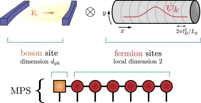
Figure 2: Cartoon for the hybrid MPS ansatz. The cavity photon is placed at the first site of the MPS, while the rest of the MPS sites represent the LLL wavefunctions $\psi_{k}$.

II.6.1 Hybrid MPS ansatz

Here we introduce a hybrid cavity-matter finite MPS ansatz where the photon is placed at the beginning of the MPS (Figure 2), also used in Refs [45, 44, 43, 46]. Empirically we observed that this MPS ansatz is still efficient enough in representing the non-local correlations of the cavity mode, provided that the bond dimension $m$ is large enough. The light-matter interactions are also easy to represent as an MPO due to their infinite range nature [70]. Here the choice of the Dipole gauge is actually important to avoid the dressing of the 4-body operators in the only matter part which can become quite expensive, differently from the dressing of 2-body operators [43]. Moreover we make an explicit use of the freedom in the choice the overall constant in the light-matter matrix elements $\kappa_{0}$ (Eq. (II.5)) such that the constraint given in Eq. (25) gives zero coherent occupation of the photon $\langle\hat{a}\rangle_{D}=0$. This guarantees a good convergence with the truncation of the cavity Hilbert space at $d_{\mathrm{ph}}=64$. Note that the total number of electrons and total momentum along $y$ are still good quantum numbers that we conserve in our simulations. We limit the bond dimension of the MPS up to $m=1600$ which allows us to keep the truncation error always below $10^{-6}$.

Apart from ground state properties via DMRG, we also focus on excited states and dynamical properties with different methods. Regarding the excited states, it is possible to directly get good results from the local effective Hamiltonians constructed during DMRG runs, as discussed in Ref. [71]. In particular local targeting of the excited states has been found to be quite accurate for critical system in 1D [71], owing the success to the delocalized nature of the low lying spectrum. As discussed more in depth in Sec. V.2 we find that this method gives good qualitative results and is even able to capture mixed light-matter polariton states. There we further study dynamical properties via time evolution with TDVP (two site updates) or directly using Lanczos methods in ED [72]. For these TDVP runs we limit the bond dimension of the MPS to $m=200$ which still guarantees good convergence for small circumferences at a reduced computational cost.

Interestingly, the TDVP algorithm can also be used to implement change of gauges via the unitary $\hat{U}$. In particular we divide $\hat{U}$ in many steps and apply them sequentially as commonly done in TDVP evolutions. The “Hamiltonian” of this gauge change is:

$$\hat{h}_{\mathrm{gauge}}=(\hat{a}+\hat{a}^{\dagger})\sum_{k}\chi_{k}\hat{n}_{k},$$ (36)

so that:

$$\hat{U}=\exp(-i\hat{h}_{\mathrm{gauge}}),$$ (37)

and, in this units, the evolution time is $\tau=1$. The fact that the MPS representation of the many-body ground state in a different gauge remains efficiently compressible (i.e., small enough bond dimension) is not guaranteed a priori and has to be checked. We find this to be case in the FQH phase. During the change of gauge we keep the bond dimension of the MPS constant.

III Topological order in cavity

\begin{overpic}[width=130.08731pt]{flux} \put(0.0,60.0){(a)} \end{overpic}  \begin{overpic}[width=130.08731pt]{sigma_16_30.pdf} \put(25.0,20.0){(b)} \end{overpic}  \begin{overpic}[width=130.08731pt]{sigmaexp_16_30.pdf} \put(25.0,75.0){(c)} \end{overpic}

Figure 3: (a) Sketch of the flux insertion; as a unit of time $\tau$ passes a unit of flux $\Phi_{0}$ is inserted resulting in relative shift in position of the cylinder along $x$. (b) Inverse resistivity in the bulk $x_{0}\in[-2,2]$ as measured by the density (Eq. (44)) with a shaded green area and quantized value $\rho_{xy}^{-1}=1/3$ as a dashed red line. At strong cavity field gradients $g$ the quantization is lost. (c) Exponential decay from the edge of density modulations $\hat{n}(x)$ around the bulk quantized value. $x=0$ is the center of the cylinder while $x=20$ is already outside of it. Obtained via DMRG at system size $L_{y}=16$ and $N_{e}=30$.

The presence of a genuine non-local degree of freedom makes the present setting not immediately classifiable within the framework of topological phases of matter. In the context of cavity mediated topology, a lot of attention has been dedicated to regimes where the cavity degree of freedom can be integrated out, both in the quantum materials context [11, 10, 21, 73] and in cold atom set-ups [74, 75, 76, 77]. Integrating out the non-local mode generally produces effective long-range interactions which simplify the picture of a mixed cavity-matter system and require the inspection of a matter-only model. This neglects by construction light-matter entanglement and give a direct interpretation of cavity mediated topology in terms of “standard” topology.

Here, we are interested in the opposite situation, where light-matter entanglement cannot be neglected - and, as we show below, does carry key signatures of topological order.

Few works [44, 78, 79, 80] have been recently investigating the questions above in the context of Symmetry Protected Topological (SPT) phases. In particular in Ref. [44] pointed out that, in the case of Majorana fermions, respecting the symmetry which protects the topology is fundamental. The FQH effect instead belongs to a fundamentally different set of topological states which display topological order - that is, where order is intrinsically related to emergent gauge theories and entanglement. Addressing the interplay of topological order and quantum light is thus a completely distinct challenge with respect to the above mentioned SPTs.

As a paradigm of FQH, we are going to study the effect of the non-local cavity degree of freedom on the topological properties of a $\nu=1/3$ Laughlin state. In particular we focus on two markers, first on the Hall resistivity (Sec. III.1) and second on the entanglement properties (Sec. III.2). They represent two key aspects of topological order: quantization of transport properties, and fingerprints in the entanglement structure of a state. Once the stability of the FQH phase is understood, we further discuss (Sec. III.3) the effect of cavity fluctuations on the emergent geometry of the FQH state.

III.1 Hall resistivity via flux insertion

A key feature of the FQH effect is the fractionally quantized transverse resistivity $\rho_{xy}$. An easy way to probe this quantity numerically on the cylinder geometry is via the so-called adiabatic flux insertion [51], sketched in Fig. 3(a).

Let us now consider the adiabatic insertion of a single magnetic flux quanta $\Phi_{0}=2\pi\hbar/e$ in the cylinder over a time $\tau$. This process can be described by a uniform time-dependent vector potential $\bm{A}_{p}(t)=\frac{\Phi_{0}}{L_{y}}\frac{t}{\tau}\bm{u}_{y}$, so that $\Phi(t)=\Phi_{0}t/\tau$. The vector potential $\bm{A}_{p}(t)$ in turns generate an electric field $\bm{E}_{p}=-\partial_{t}\bm{A}_{p}=\frac{\Phi_{0}}{\tau L_{y}}\bm{u}_{y}$, which is constant in time and directed towards the $y$ direction. Hence, we can find the Hall resistivity by calculating the current $\hat{J}_{x}=\hat{\bm{J}}\cdot\bm{u}_{x}$ flowing transversely to the electric field $\bm{E}_{p}$. Since our system is homogeneous in $y$ but in general not along $x$ the result is a spatial dependent resistivity:

$$\rho_{xy}(x)=\frac{E_{y}}{e\langle\hat{J}_{x}(x)\rangle}.$$ (38)

For the FQHE the bulk value is expected to be quantized as $\rho_{xy}=\frac{1}{\nu}\frac{h}{e^{2}}$ with $\nu=1/3$ in this work.

In the adiabatic limit $\tau\rightarrow\infty$ and assuming the existence of a many-body gap, we can focus on the ground state of the instantaneous total Hamiltonian $\hat{H}(\Phi)$ which in principle depends on $\Phi$. Now we know that a constant vector potential $\bm{A}_{p}$ does not couple to the LLL. Indeed, the effect of a flux $\Phi$ is to change the $y$-momentum quantization of the single particle orbitals $\psi_{n,k}$ (Sec. II.1) and consequently their position:

$$k_{\Phi}=\frac{2\pi}{L_{y}}m_{k}+\frac{2\pi}{L_{y}}\frac{\Phi}{\Phi_{0}},\qquad X_{k_{\Phi}}=k_{\Phi}\,l_{B}^{2}$$ (39)

with $m_{k}\in\mathbb{Z}$. This means that the projection $\mathcal{P}_{\Phi}$ to the LLL depends on $\Phi$. This is not an issue as long as we focus on adiabatic processes. Given Eq. (39), we can now inspect how the many-body light-matter Hamiltonian $\hat{H}(\Phi)$ looks like. The electron-electron interaction clearly remains unchanged as it only depends on difference of momenta. The light-matter coupling, for this purpose, is more conveniently formulated within the Coulomb gauge formulation (Sec. II.3). Here the interaction is only controlled by difference in momenta $k_{\Phi}-k_{\Phi}^{\prime}$ and hence the full Hamiltonian $\hat{H}(\Phi)$ remains unchanged. As a key consequence we have that the ground state wavefunction in second quantization $\ket{\mathrm{GS}_{\Phi}}$, hence fixing an orbital basis, will be the same:

$$\hat{H}(\Phi)\equiv\hat{H}(\Phi=0)\;\;\Rightarrow\;\;\ket{\mathrm{GS}_{\Phi}}\equiv\ket{\mathrm{GS}_{\Phi=0}}.$$ (40)

It is important to stress that in Eq. (40), we have not used the equality sign. The reasons is that the Hilbert spaces in which the two sides of the equations are defined are not, strictly speaking, the same: they refer to different LLL projection $\hat{\mathcal{P}}_{\Phi}$. In order to perform a meaningful comparison, we can consider relevant physical observables such as the charge density $\hat{n}(x)$, which is expressed as:

$$\hat{n}(x)=\frac{1}{L_{y}}\sum_{k_{\Phi}}\hat{n}_{k_{\Phi}}|\phi_{0}(x-X_{k_{\Phi}})|^{2},$$ (41)

and can be evaluated at different $\Phi$ by just using the $\Phi=0$ solution with a change in the single particle orbitals $\phi_{0}(x-X_{k_{\Phi}})$.

In order to calculate the current $\langle\hat{J}_{x}\rangle$ we use the continuity equation:

$$\bm{\nabla}\cdot\langle\hat{\bm{J}}\rangle=\partial_{t}\langle\hat{n}\rangle,$$ (42)

where $\hat{\bm{J}}$ is the current operator. Given our finite cylinder geometry we can integrate both sides of the equation above in a region $\mathcal{V}=\{(x,y)\,\mathrm{s.t.}\ x<x_{0}\}$ to get:

$$\langle\hat{J}_{x}(x_{0})\rangle=\partial_{t}\int_{-\infty}^{x_{0}}\differential x\langle\hat{n}(x)\rangle_{\Phi(t)}$$ (43)

with $\hat{J}_{x}(x_{0})$ the current density along $x$ at position $x_{0}$. Because of translational invariance on $y$ the current and the density do not depend on $y$ making the integration over $y$ trivial. Using Eq. (41) and the ramp protocol $\Phi(t)\propto t$ we can express the local transverse resistivity in terms of the static density:

$$\rho_{xy}(x_{0})=\frac{1}{2\pi\langle\hat{n}(x_{0})\rangle}\frac{h}{e^{2}},$$ (44)

with $h/e^{2}$ being the Von Klitzing constant and the factor $2\pi$ is the area occupied by a single-particle state (in units of $l_{B}^{2}$). The above equation directly links the bulk density to the fractional Hall response of the system. In particular for a topologically ordered state in the class of the Laughlin $1/3$ one expects the bulk density to be constant $2\pi\langle\hat{n}(x_{0})\rangle=1/3$.

In Fig. 3(b) we show the bulk resistivity ($x_{0}\in[-2,2]$) as a function of cavity field gradients $g$ for a specific system size ($L_{y}=16$, $N_{e}=30$). The resistivity is quantized up to exponential corrections even at relatively large values of the cavity field gradient $g\simeq 2$. The nature of the ground state in the regime of non-quantized Hall response will be better characterized in Sec IV. In Fig. 3(c) we depict the deviations of the density from its bulk value when approaching an edge of the cylinder ($x=0$ is the center of the system while $x=20$ is outside of it). For all depicted couplings in the FQH phase, the corrections decay exponentially in the bulk with a correlation length $l_{\mathrm{edge}}$ which increase with $g$.

It has been recently argued [22] that the finite lifetime of the cavity mode can give a correction to the quantized transverse conductivity at temperature $T=0$ in the IQH regime. We note that at the many-body level the flux insertion argument can be adapted to the case of weak cavity losses (see Appendix A). The key physical insight is that the steady state of the whole system (cavity+matter) is at thermal equilibrium with the bath [81], hence the ground state results regarding the Hall resistivity are expected to hold provided that the photonic bath is at a small enough temperature. It would be interesting to check, in the spirit of Ref. [22], what finite temperature corrections are. We leave this to future work.

III.2 Entanglement spectrum

\begin{overpic}[width=127.9171pt]{entspectrum_20_34_L.pdf} \put(20.0,65.0){(a)} \end{overpic}

\begin{overpic}[width=127.9171pt]{entspectrum_20_34.pdf} \put(20.0,20.0){(b)} \end{overpic}

\begin{overpic}[width=155.66676pt]{entspectrumC_20_34.pdf} \put(17.0,17.0){(c)} \end{overpic}

Figure 4: Entanglement spectra obtained via DMRG for the asymmetric bipartition of Eq. (47) on system size $L_{y}=20$ and $N_{e}=34$. The charge sector of the shown spectra is $N_{e}/2=17$ while the momentum along $y$ gives the x-axis. In panel (a) the state is pure Laughlin ($g=0$) while in panel (b,c) we have a finite light-matter coupling $g=0.2$ in Dipole and Coulomb gauge respectively. The color represent the number of photons in each Schmidt state and the colorbar is the same for all three panels

The entanglement spectrum at bipartition of a topologically ordered state can be used to detect topological order [33, 82, 38, 83]. In particular, one expect to find information about the edge theory of the topological state under consideration. This procedure, dubbed entanglement spectroscopy, is widely used as a theoretical tool and has also been also proposed as an experimental protocol to detect topology in cold atom systems [83]. The deep roots of this topology-entanglement connection lie in a very general results in relativistic quantum field theory, the Bisognano-Wichmann theorem [84, 85], which dictates closed functional form expressions for the entanglement (or modular) Hamiltonian, and explain the Li-Haldane result [86]. A natural question to ask is, what is left about this topology footprint on entanglement in the presence of quantum light.

Before discussing our hybrid cavity-matter setting, we review some general concepts. Let us define the pure state $\ket{\Psi}$ of the full system and the density matrix $\hat{\rho}_{A}$ of a subsystem $A$ as $\hat{\rho}_{A}=\Tr_{B}\left[\ket{\Psi}\bra{\Psi}\right]$ with $B$ being the rest of the system. In general, we can write:

$$\hat{\rho}_{A}=\exp\left(-\hat{H}_{ee}\right)=\exp\left(-\sum_{{q},i}\xi_{\{q\},i}\ket{\phi_{\{q\},i}}\bra{\phi_{\{q\},i}}\right),$$ (45)

where $\hat{H}_{ee}$ is the entanglement Hamiltonian, $\xi_{\{q\},i}$ the entanglement energies, $\ket{\phi_{\{q\},i}}$ the Schmidt vectors corresponding to the bipartition, and $(\{q\},i)$ an index tuple labeling the quantum numbers $\{q\}$ and the Schmidt state $i$. Following the Li-Haldane conjecture [33, 34], the entanglement spectrum for a bipartition in the bulk must follow, at low energies, the Hamiltonian of the edge. For Laughlin states, the edge theory is a chiral Luttinger liquid ($\chi$LL) [87, 88] which, once the $U(1)$ charge sector is fixed, gives a specific fingerprint in terms of degeneracies at each total momentum:

$$(d_{0},d_{1},d_{2},d_{3},d_{4},d_{5},\dots)=(1,1,2,3,5,7,\dots),$$ (46)

with $d_{k}$ being the degeneracy at momentum quantum number $k$. At finite sizes, the degeneracies are usually broken but a gap still separate a universal low energy part from a non-universal part of the entanglement spectrum [34]. This remark that this also happens for energy spectra at physical edges [89] and not only for entanglement spectra in bulk bipartitions.

In the case of a cavity embedded systems there is no clear notion of pure state bipartition as the non-local bosonic mode cannot be “divided” in two. As already done in [44, 45], one needs to define asymmetric bipartitions where the cavity mode resides on one side. A possible choice is the following:

$$\hat{\rho}_{X_{k}>0}=\Tr_{x<0;c}\left[\ket{\Psi}\bra{\Psi}\right]$$ (47)

where $\ket{\Psi}$ is the many-body ground state, $\hat{\rho}_{X_{k}>0}$ is the reduced density matrix for electrons in orbitals $k$ with $X_{k}>0$ and $\Tr_{X_{k}<0;c}$ is the trace over electrons at $X_{k}<0$ and the cavity mode $c$. One can, however, always recover the notion of an only matter bipartition by considering the electronic density matrix $\hat{\rho}_{el}=\Tr_{c}[\ket{\Psi}\bra{\Psi}]$. Taking its bipartition will give as a result the same density matrix of the asymmetric bipartition with the cavity in Eq. (47).

In light of the discussion about different possible representations of the cavity-matter system (Sec. II.3), we want to stress that (not unexpectedly) the entanglement spectrum is not a gauge invariant quantity. Indeed, it can change under global unitary transformations $\hat{U}$ which implement the change of gauge, since a global change of basis can change the reduced density matrix of subsystems. However, as discussed in Sec. II.6, we can easily change the gauge in which a state $\ket{\Psi}$ is represented by applying the unitary $\hat{U}$ and just check whether the entanglement spectrum displays features that are stable against the change of gauge.

III.2.1 Entanglement spectrum bands and polariton entanglement gap

In Fig. 4 we show the DMRG results for the entanglement spectrum of the asymmetric bipartition in Eq. (47) at $g=0$ (a) and at finite $g=0.2$ in the Dipole (b) and Coulomb (c) gauges. In particular, we fix the number of particles of the bipartition to be $N_{e}/2$ and look at momentum quantum number $K_{y}$. At finite light-matter coupling $g$ the entanglement spectrum still show the $\chi$LL counting, but the higher energy part clearly changes. In order to understand the difference between entanglement eigenvectors, we color the dots based on the number of photons in the respective Schmidt state:

$$n^{ph}_{\{q\},i}=\bra{\phi_{\{q\},i}}\hat{a}^{\dagger}\hat{a}\ket{\phi_{\{q\},i}},$$ (48)

where the Schmidt states are readily available from the total MPS. This highlights a very informative pattern. The $\chi$LL counting is repeated for number of photons roughly equals to integers. We empirically find for each of these branches:

$$n^{ph}_{k,j}\simeq j,\qquad\xi_{k,j}\simeq\epsilon_{k}+j\Delta_{pol},$$ (49)

with $\epsilon_{k}$ being a size dependent non-universal dispersion and $j=0,1,2,\dots$ being an integer. The quantity $\Delta_{pol}$, which we call polariton entanglement gap, controls the separation between different sectors of the $\chi$LL with different number of photons and needs to be finite to preserve the $\chi$LL structure.

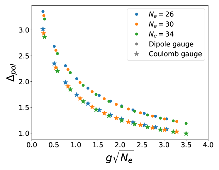
Figure 5: Polariton entanglement gap extrated from DMRG entanglement spectra in the middle of the cylinder for different number of particles $N_{e}$ in the Dipole gauge (circles) and Coulomb gauge (stars) as a function of the collective coupling $g\sqrt{N_{e}}$. $L_{y}=20$

In Fig. 5 we study the polariton entanglement gap dependence with system size. We show its dependence as a function of a re-scaled collective coupling $g\sqrt{N_{e}}$ for different number of particles $N_{e}$. The perfect collapse highlights the collective nature of polariton excitations, i.e., they are controlled by the collective coupling $g\sqrt{N_{e}}$. By showing the entanglement gap for both gauges it is evident that this is a gauge dependent quantity, nonetheless both gauges reveal the same collective behavior. Moreover, we find that the value of $\Delta_{pol}$ does not depend on $L_{y}$ (not shown).

The nature of this gapped polaritonic excitation will be clarified in Sec. V, where we show that a strong hybridization between a collective emergent electronic mode, the $q\simeq 0$ part of the magnetoroton spectrum, and the cavity is taking place. An important consequence of the collective coupling is that taking thermodynamic limit $N_{e}\rightarrow\infty$ at fixed $g$ breaks the $\chi$LL counting and the topological order of the state. The stability of the FQH phase at finite $g$ then needs to be understood in a mesoscopic sense – another important scale $g\sqrt{N_{e}}$ is controlling the many-body gap of the FQH phase and hence its topological order.

III.3 Cavity control of FQH geometry

Another important property of a FQH state which have received a lot of interest in recent years is its intrinsic geometry or metric [29, 30, 31, 90, 91]. This controls many of its ground state correlations and its long-wavelength gapped excitations quanta, in analogy with gravitational theories that have been dubbed as “gravitons” [30, 31, 32]. Here we focus on ground state leaving for Sec. V the discussion about excitations.

A key ground state footprint of non-trivial geometry can be found in guiding-center correlations [92, 91], in particular via the guiding-center structure factor $S(\bm{q})$ - see Eq. (33) - at small momenta. For a gapped FQH state it is possible to show [92, 91] that:

$$S(\bm{q})\simeq S_{4}^{xx}q_{x}^{4}+2S_{4}^{xy}q_{x}^{2}q_{y}^{2}+S_{4}^{yy}q_{y}^{4}.$$ (50)

In the case of unbroken rotational invariance, we further have $S_{4}^{xx}=S_{4}^{xy}=S_{4}^{yy}=s_{4}$, with $s_{4}$ satisfying the Haldane bound $s_{4}\geq(1-\nu)/24\nu$ saturated by the Laughlin state [92, 93]. Anisotropic interactions and/or anisotropic LLs [29] induce an intrinsic anisotropic geometry on the FQH liquid.

\begin{overpic}[width=433.62pt]{S4xx.pdf} \end{overpic}

Figure 6: Long wavelength static structure factor parameter $S^{xx}_{4}$ as a function of the collective coupling $g\sqrt{N_{e}}$ for different number of electrons $N_{e}$ at fixed cylinder circumference $L_{y}=20$. The black dashed line represent the Haldane bound $s_{4}=(1-\nu)/24\nu$ valid for isotropic interactions and saturated by the Laughlin at $g=0$ in the thermodinamic limit. Inset: Static structure factor as a function of momenta along $y$ for $g=0$ (red) and $g=1$ (blue) showing enhancement of the small wavevector part. The dashed red line represent the thermodinamic limit behaviour $S(q_{y})=s_{4}\;q_{y}^{4}$ of the Laughlin state.

In Fig. 6 we show the effect of cavity fluctuations on the long-wavelength properties of $S(\bm{q})$. The behaviour for momenta along $x$ is still quartic and the proportionality factor $S_{4}^{xx}$ is plotted against the collective coupling $g\sqrt{N_{e}}$. To extract it we directly look at the definition of $S(q_{x})$ and expand for small $q_{x}$:

$$S_{4}^{xx}=\lim_{q_{x}\rightarrow 0}\frac{1}{4!}\partial_{q_{x}}^{4}S(q_{x})=\frac{1}{4M}\sum_{k,k^{\prime}}k^{2}k^{\prime 2}\langle\delta\hat{n}_{k}\delta\hat{n}_{k^{\prime}}\rangle,$$ (51)

with $\delta\hat{n}_{k}=\hat{n}_{k}-\langle\hat{n}_{k}\rangle$. Finite size effect with both $N_{e}$ and $L_{y}$ are expected and are signaled by the discrepancy with the known value $s_{4}=(1-\nu)/24\nu$ at $g=0$ shown as a dashed black line. Nonetheless the finite $g$ reduction is consistent and likely hold in the thermodynamic limit. The extraction of all three parameters in Eq. (50) is hindered by strong finite size effects along $y$. This is highlighted in the inset of Fig. 6 where we show the full dependence of $S(q_{y})$ which cannot capture the $q_{y}^{4}$ dependence. Qualitatively we still see that correlations along $y$ are enhanced at finite $g$, as opposed to those on $x$.

\begin{overpic}[width=132.25092pt]{density_16_30.pdf} \put(20.0,75.0){(a)} \end{overpic}

\begin{overpic}[width=147.4292pt]{g2_fqh_20.pdf} \put(20.0,70.0){(c)} \end{overpic}

\begin{overpic}[width=132.25092pt]{Sord_20.pdf} \put(20.0,75.0){(e)} \end{overpic}

\begin{overpic}[width=132.25092pt]{density_20_30.pdf} \put(20.0,75.0){(b)} \end{overpic}

\begin{overpic}[width=147.4292pt]{g2_fqh_80.pdf} \put(20.0,70.0){(d)} \end{overpic}

\begin{overpic}[width=132.25092pt]{cavityord_20.pdf} \put(20.0,75.0){(f)} \par\end{overpic}

Figure 7: Left panels (a,b) show the orbital occupancies from Laughlin state at $g=0$ (red) to stripe phase at $g=3$ (blue) for two circumferences of the cylinder $L_{y}=16$ (a) and $L_{y}=20$ (b) at fixed $N_{e}=30$. Note that at fixed number of particles the size of the system along $x$ reduces. Center panels (c,d) show the densisty-density correlations $G^{(2)}(0,\bm{r})$ in the two phases, at $g=1$ for the FQH phase in panel (c) and at $g=4$ for the stripe phase in panel (d). In the FQH phase (panel (c)) we also compare the shape of the correlation hole between $g=1$ (white line) and the Laughlin $g=0$ (blue line) by tracking the local maximum of the $G^{(2)}$. For both panels (c,d) $L_{y}=20$ and $N_{e}=34$. Right panels (e,f) show the behaviour of two quantities across the transition for different $N_{e}$ and fixed $L_{y}=20$. Panel (e) show the peak height of the static structure factor as defined in the main text and serve as an order parameter. Panel (f) show the electric field fluctuations (full lines) and the contribution coming from the polarization (dashed lines).

Another key signature of a distorted metric is the shape of the correlation hole of the $G_{2}$, shown in Fig. 7(c) for $g=1$ (white line) and compared with the circular one of the $g=0$ Laughlin case (blue line). As already noticed for other anysotropic FQH model wavefunctions [94], we also find that the short distance behaviour of the $G_{2}(r)$ changes from $r^{6}$ to $r^{2}$ going from isotropic ($g=0$) to anisotropic cases ($g>0$). We also note that the effect at long wavelength shown in Fig. 6 is greater in magnitude with respect to the reshaping of the correlation hole. As a rule of thumb, we expect the latter to be more sensible to short wavelength properties (electron-electron interactions) while the former to long-wavelength (cavity-mediated interactions). We suggest this to be related to the cavity induced modifications of the magnetoroton dispersion (Sec. V) which are collectively enhanced ($g\sqrt{N_{e}}$) only around the graviton part $q\to 0$ while at finite $q$ seems only to see the single-particle coupling ($g$). This is intuitively related to the fact that a uniform field gradient couples collectively to a uniform quadrupolar excitation, the graviton ($q\to 0$), and not to quadrupolar excitations at finite momenta, the rest of the magnetoroton dispersion ($q$ finite).

IV Cavity-induced sliding Tomonaga-Luttinger liquid

In this section, we analyze the nature of the large coupling regime $g\gtrsim 1$. In particular we first provide numerical evidence for a cavity mediated instability to a stripe phase with strong density modulation along the $x$ direction (Sec. IV.1). Then we argue on the basis of a mean-field argument how the squeezed geometry analyzed in Sec III.3 is stabilizing the FQH phase, pushing the transition to higher values of the coupling $g$ (Sec. IV.2). Finally, we complete the understanding of the strong coupling phase as a sliding Tomonaga-Luttinger liquid and discuss the effect of fluctuations (Sec. IV.3).

IV.1 Numerical results

In Fig. 7 we present a sample of the numerical results obtained via DMRG simulations as discussed in Sec. II.6. In order to get immediate insight on the state of the system we can look at the orbital density $\hat{n}_{k}$ in the left panels (a) and (b). The Laughlin state ($g=0$ red line) shows a quantized bulk density $\hat{n}_{k}$ with modulations only close to the edge due to the open boundaries. A strong bulk modulation instead appears around $g\simeq 2-3$ for both system sizes $L_{y}=16$ and $L_{y}=20$. The modulation in orbital space follows a different pattern for the two system sizes. In particular, we have that the number of electron per peak are $n_{S}=3$ and $n_{S}=4$ for system system sizes $L_{y}=16$ and $L_{y}=20$ respectively. In order to understand this we recall that the distance between two neighboring orbitals decreases as $\Delta X_{k}=2\pi/L_{y}$. Hence to keep the distance between the peaks $\lambda_{S}$ independent of $L_{y}$, the number of particle per peak $n_{S}$ must increase. This constrains the generic behavior of $\lambda_{S}$ to be

$$\lambda_{S}=\frac{2\pi}{L_{y}}3n_{s}(L_{y}),$$ (52)

where we expect $n_{s}(L_{y})\propto L_{y}$ in the thermodynamic limit.

In order to check the 2D stripe nature of the phase we show the density-density correlator $G^{(2)}(\bm{r}_{1},\bm{r}_{2})$ in the center panels (c) and (d) as defined in Eq. (31). In the FQH phase ($g=1$ panel (c)) we find the characteristic correlation hole at short distances and a constant value at long distances as one should expect from a liquid state. Note that, as discussed in Sec. III.3, the anisotropic nature of the cavity mode reflects into an anisotropic correlation hole. To highlight this, two lines are shown which tracks the maximum of the $G^{(2)}$, one for the Laughlin at $g=0$ (blue line) and one for the $g=1$ case (white line) whose $G^{(2)}$ is actually plotted. In the strong coupling regime instead ($g=4$ panel (d)) there is clear ordering on $x$ and absence of ordering on $y$, confirming the interpretation of the phase as stripe phase. Weak density modulations on $y$ are present within the stripe, likely due to finite size effects and not to a true crystalline order in 2D.

In the right panels (e,f) we show two quantities related to the matter and cavity components. For the electrons we consider the maximum of the disconnected static structure factor $S_{uc}(\bm{q})$ at finite momenta where it is expected to scale with $N_{e}$ in a charge density wave phase and not in a liquid phase. $S_{uc}(\bm{q})$ is defined as in $S(\bm{q})$ (Eq. (33)) but with the full guiding center density operator $\hat{\bar{\rho}}(\bm{q})$ replacing fluctuations $\delta\hat{\bar{\rho}}(\bm{q})$ in the definition. Panel (e) shows the normalized finite-momenta peak height of the disconnected static structure factor $\max S_{uc}(\bm{q})/N_{e}$ which is found around $\bm{q}\simeq(1.75,0)$. At fixed $L_{y}$ the transition point seems to shift towards higher values of $g$ with increasing $N_{e}$. However, a more careful investigation is hindered by commensurability effects on $y$ which likely renormalize the energy cost of the stripes for finite $L_{y}$. We note that considering the thermodynamic limit in the $x$ direction with an infinite MPS is impossible with the present cavity-matter structure.

For the cavity mode, we consider the scalar electric field $\hat{E}$ (Eq. (22)). Since its expectation value vanishes identically because of Eq. (25), we look at its fluctuations in panel (f) as a function of $g$ for different system sizes (full lines). There we also show how, in the Dipole gauge, most of the fluctuations come from the $\hat{P}^{2}$ term (dashed lines). The terms $\hat{D}\hat{P}$ and $\hat{D}^{2}$ are still macroscopic even though they almost cancel each other. Fluctuations peak in the vicinity of the value of $g$ where strong stripe order forms and decrease afterwards. This indicate a crucial role of vacuum electric field gradient fluctuations in driving the instability.

IV.2 Photon mean-field argument

In order to get an insight of the effect of the field gradients we perform a mean-field decoupling of the photon and matter degrees of freedom in the Dipole gauge. Due to the linear nature of the coupling term, the mean-field state generally reads:

$$\ket{\Psi}=\ket{\alpha}\ket{\psi},$$ (53)

with $\ket{\psi}$ being an electronic wavefunction defined on the LLL and $\ket{\alpha}$ being a coherent state. Minimizing the mean-field state energy over the coherent state value gives:

$$\alpha=i\sum_{k}\chi_{k}\bra{\psi}\hat{n}_{k}\ket{\psi}.$$ (54)

In order to find the best mean-field ansatz, one should then take the photon mean-field Hamiltonian for the electrons:

$$\hat{H}_{\mathrm{PMF}}=\hat{H}_{\mathrm{int}}+\omega_{c}\left[\sum_{k}\chi_{k}\big{(}\hat{n}_{k}-\bra{\psi}\hat{n}_{k}\ket{\psi}\big{)}\right]^{2},$$ (55)

and find the ground state $\ket{\psi}$ with a self-consistent procedure [43].

This minimization still requires the solution of a complicated many-body Hamiltonian. However we can now clearly see two different terms competing, the first is the electron-electron interaction and the second is due to effective cavity mediated interactions. The latter has a very specific form: e.g., when calculated on the ground state $\ket{\psi}$, it is the variance of the polarization operator $\hat{P}$. This has two important consequences. First it is a positive number and second it is, in general, an extensive quantity, being proportional to $N_{e}$. These are not specific to the FQH set-up, but a more general property of Dipole gauge Hamiltonians where the so-called self polarization term is present. For other models where only the linear coupling is present, e.g., the Dicke model, the all-to-all nature of the mode leads to collective enhanced cavity-mediated interactions which contribute superextensively, and grow as $g^{2}N_{e}^{2}$. For this reason one can usually work with a collective coupling $g\sqrt{N_{e}}$. Here instead we clearly see that the cavity mediated interactions are controlled by the so-called single particle coupling constant $g$.

We can now discuss two limiting cases: $g=0$ and $g\rightarrow\infty$. In the first case, we recover a pure Laughlin state, eigenstate of the first part of the Hamiltonian. In the second case instead, there will be a massive degeneracy of states with no fluctuations of the polarization operator $\hat{P}$ lifted only by the interactions $\hat{H}_{\mathrm{int}}$. All product states in the orbital basis will, for example, have no orbital density fluctuations and hence give identically zero contributions to the second term. Among these states we can write down stripe states with index $n$:

$$\ket{S_{n}}=\ket{\{0_{n}1_{n}0_{n}\}},$$ (56)

where $0_{n}$ ($1_{n}$) indicates the repetition of zero (one) electron in $n$ consecutive orbitals and the curly bracket indicate the repetition of such unit cell. Note that these states satisfy the bulk filling factor $1/3$ by construction. The electron-electron interaction energy contribution of these states is also relatively simple to calculate. The mean-field energy of the stripe state $\ket{S_{n}}$ is:

$$E_{S_{n}}=\bra{S_{n}}\hat{H}_{\mathrm{int}}\ket{S_{n}}=\sum_{k_{1},k_{2}\in K_{\mathrm{occ}}}2V_{k_{1},k_{2},k_{2},k_{1}},$$ (57)

where $K_{\mathrm{occ}}$ is the set of orbitals which are occupied in $\ket{S_{n}}$, and $V_{k_{1},k_{2},k_{2},k_{1}}$ are matrix elements given by Eq. (II.1). By changing the circumference of the cylinder $L_{y}$ the energy per particle will also change, as shown in Fig. 8. For each number of particle per stripe $n$ there is an $L_{y}$ that minimizes the mean-field energy and this increases with $n$.

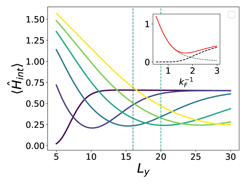
Figure 8: Interaction energy of stripe state $\ket{S_{n}}$ in the photon mean-field approximation with $n$ going from $n=1$ (dark blue) to $n=6$ (yellow) as a function of cylinder circumference $L_{y}$ size. Dashed vertical lines show that for $L_{y}=20$ and $L_{y}=16$ used in Fig. 7 the states with $n=4$ and $n=3$ are favoured. Inset: approximate behavior of $E_{S_{n}}$ as a function of $1/k_{\mathrm{F}}\simeq L_{y}/3n$ in the thermodynamic limit. The two main contributions to the interaction energy, same stripe (dotted) and neighboring stripes (dashed), sum up to $E_{S_{n}}$ (red full line). The minimum is around $k_{\mathrm{F}}^{-1}\simeq 1.6$ ($\lambda_{S}\simeq 5$).

This behavior can be well understood by working in the thermodynamic limit $L_{y}\to\infty$. In this setting, the stripe state can be essentially viewed as an array of filled Fermi seas, each with Fermi momentum $k_{\mathrm{F}}=\pi n/L_{y}$, and whose centers are separated in momentum by $\Delta k=6k_{\mathrm{F}}$. The circumference $L_{y}$ controls the range of the electron-electron interactions $V_{k_{1},k_{2},k_{2},k_{1}}$ on the momentum basis via an exponential $\propto e^{-(k_{1}-k_{2})^{2}/2}$. Thus, if we start from small $L_{y}$, i.e., large $k_{\mathrm{F}}$ for some $n$ fixed, the most prominent contribution to $E_{S_{n}}$ must come from interactions between electrons living on the same stripe. Then, by increasing $L_{y}$, interactions among electrons on different stripes are expected to become stronger. We thus expand the energy $E_{S_{n}}$ as the sum

$$E_{S_{n}}=E_{S_{n}}^{(0)}+E_{S_{n}}^{(1)}+\cdots,$$ (58)

where $E_{S_{n}}^{(0)}$ and $E_{S_{n}}^{(1)}$ respectively represent the energy contributions of electrons on the same and nearest neighbor stripes. Taking the continuum limit $\sum_{k}\to\frac{L_{y}}{2\pi}\int\differential k$, we estimate these two energy contributions (details on appendix B) to be

$$E_{S_{n}}^{(0)}=2N_{e}\Big{[}\erf(\sqrt{2}k_{\mathrm{F}})+\frac{2e^{-2k_{\mathrm{F}}^{2}}-2}{\sqrt{2\pi}k_{\mathrm{F}}}\Big{]},$$ (59)

and

$$E_{S_{n}}^{(1)} =4N_{e}\Big{[}\erf(\sqrt{8}k_{\mathrm{F}})-3\erf(\sqrt{18}k_{\mathrm{F}})+2\erf(\sqrt{32}k_{\mathrm{F}})$$

$$+\frac{e^{-8k_{\mathrm{F}}^{2}}-2e^{-18k_{\mathrm{F}}^{2}}+e^{-32k_{\mathrm{F}}^{2}}}{\sqrt{2\pi}k_{\mathrm{F}}}\Big{]},$$ (60)

where $\erf(x)$ is the Gauss error function. In Fig. 8(b) we plot the approximate form of $E_{S_{n}}$ as a function of $1/k_{\mathrm{F}}$. Within this approximation, we find the minimum lies at $k_{\mathrm{F,{min}}}\simeq 0.62$, with a corresponding energy gap $E_{S_{n}}/N_{e}\simeq 0.25$. This means the number of electrons per stripe $n_{S}\approx L_{y}/5$ is only dictated by $L_{y}$ in the thermodynamic limit as discussed above, see Eq. (52).

On the other hand we have that the Laughlin state $\ket{\Psi_{L}}$ is an eigenstate of $\hat{H}_{\mathrm{int}}$ with zero energy. This means the variational energy of the Laughlin state depends only on the light-induced interaction:

$$E_{L}=\omega_{c}\sum_{kk^{\prime}}\chi_{k}\chi_{k^{\prime}}\bra{\Psi_{L}}\delta\hat{n}_{k}\delta\hat{n}_{k^{\prime}}\ket{\Psi_{L}},$$ (61)

where we have defined $\delta\hat{n}_{k}=\hat{n}_{k}-\bra{\Psi_{L}}\hat{n}_{k}\ket{\Psi_{L}}$. Given that $\chi_{k}\propto k^{2}$, it is possible to compute this energy contribution via the long-wavelength behaviour of the static structure factor $S(\bm{q})$. From Eq. (51), we observe that $E_{L}$ is directly tied to the $S_{4}^{xx}$ component, so when we send $N_{e}\to\infty$, the mean-field energy scales as

$$E_{L}/N_{e}\approx S_{4}^{xx}\omega_{c}g^{2}/\nu,$$ (62)

where $\nu=1/3$.

The outcome is that a transition to the stripe phase must take place once the energy of the Laughlin state $E_{L}$ becomes equal or larger than the energy $E_{S_{n}}$. Replacing the value for the unperturbed Laughlin state, $S_{4}^{xx}=(1-\nu)/24\nu$, we find the magnitude of the critical point $g=g_{\star}$ goes as $\omega_{c}g_{\star}^{2}\approx 1$. This is far below the observed values in the numerics, which happen close to $g\simeq 3$. One key reason behind this difference is the renormalization of $S_{4}^{xx}$ as a function of the light-matter interaction as shown in Fig. 6. Given $S_{4}^{xx}$ becomes smaller, the energy of the real ground state scales slower than $g^{2}$, and the transition is pushed towards a higher value of $g$. In particular, by using the numerical data for $S_{4}^{xx}$ as a function of $g$, we have checked the true ground state energy agrees well with the formula in Eq. (62). The strong resilience of the FQH liquid to cavity fluctuations is then to be attributed to the change in its geometry, interpreted as a hidden variational parameter [29].

IV.3 Field theory for the sliding Tomonaga-Luttinger liquid phase

To further clarify the nature of the sliding Tomonaga-Luttinger liquid phase [95, 96, 97], we build a set of low-energy excitations on top of our mean-field ground state. In the large light-matter coupling limit, we assume the energy penalty to introduce $\delta n_{k}$ fluctuations is so large we can only spare to build excitation with definite density occupation $n_{k}=0,1$. This is a great simplification that essentially allow us to treat the LLL electrons as an array of Tomonaga-Luttinger liquids. This state is naturally gapped along $x$, but remain gapless along the $y$ direction, and can be viewed as an archetype of a smectic metal state [95], a state with zero shear modulus [98]. The gapless modes take the form of particle-hole excitations near the Fermi points of each stripe $k_{\sigma}=\pm k_{\mathrm{F}}+6k_{\mathrm{F}}\sigma$, where $\sigma=0,\pm 1,\pm 2,\dots$ denotes the stripe index. To verify this, we first consider a particle excitation with momentum $k=k_{\mathrm{F}}+q$, assuming $q\ll k_{\mathrm{F}}$ so the excitation lies close to the right Fermi point of the stripe $\sigma=0$. In this limit, similar to the analysis carried out in Appendix B, we approximate the energy cost of adding one electron by the integral:

$$\varepsilon(k_{\mathrm{F}}+q) \simeq\sqrt{\frac{2}{\pi}}\int_{-k_{\mathrm{F}}}^{k_{\mathrm{F}}}\differential k(k_{\mathrm{F}}-k+q)^{2}e^{-\tfrac{1}{2}(k_{\mathrm{F}}-k+q)^{2}},$$ (63)

where we integrate over the nearest stripe only, throwing out energy contributions from distant stripes that are suppressed by the exponential factor. Evaluating the integral in the limit $q\to 0$, we find the linear dispersion relation $\varepsilon(k_{\mathrm{F}}+q)\approx\varepsilon(k_{\mathrm{F}})+v_{\mathrm{F}}q+\cdots$, where $v_{\mathrm{F}}=\sqrt{\frac{2}{\pi}}4k_{\mathrm{F}}^{2}e^{-2k_{\mathrm{F}}^{2}}$ plays the role of the Fermi velocity.

It thus follows that the particle-hole excitation $c_{k+q}^{\dagger}c_{k}\ket{S_{n}}$ in the vicinity of the Fermi level has a dispersion relation of the form

$$\omega(q)\approx v_{\mathrm{F}}|q|+\cdots.$$ (64)

This behavior is compatible with a sliding Tomonaga-Luttinger liquid (sTLL) model description of the stripe phase, characterized by the following low-energy Hamiltonian:

$$H_{\mathrm{sTLL}}=\sum_{\sigma}\frac{v}{2}\int\differential y\Big{[}K(\partial_{y}\theta_{\sigma})^{2}+\frac{1}{K}(\partial_{y}\phi_{\sigma})^{2}\Big{]},$$ (65)

where the boson fields $\phi_{\sigma}$ represent phase fluctuations of the charge density along each stripe $\sigma$, denoted as $\delta\hat{n}_{\sigma}=-\partial_{y}\phi_{\sigma}/\sqrt{\pi}$, and the Luttinger parameter $K$ embodies generic intra-stripe interactions. The effective model has a large (scaling with $L_{x}$) number of additional $U(1)$ symmetries, corresponding to separate number conservation on each stripe. This is reflected in the invariance of the sTLL Hamiltonian under discrete sliding transformations [98] of the form

$$\phi_{\sigma}(y)\to\phi_{\sigma}(y)+f_{\sigma},$$ (66)

where $f_{\sigma}$ is an arbitrary function over discrete values $\sigma$.

Let us now reintroduce light-matter interactions. We proceed phenomenologically, adding the cavity term $\delta H_{c}=\omega_{c}\hat{a}^{\dagger}\hat{a}$, and then performing the dipole-gauge shift: $\hat{a}\to\hat{\mathfrak{a}}=\hat{a}-i\sum_{\sigma}\chi_{\sigma}\int\differential y\,\delta\hat{n}_{\sigma}(y)$, where $\chi_{\sigma}$ takes into account field variations along the $x$ direction. Thus all cavity-related couplings are summarized into $\delta H_{c}=\omega_{c}\hat{\mathfrak{a}}^{\dagger}\hat{\mathfrak{a}}$, which we add to the sTLL Hamiltonian Eq. (65). However, as it couples individually to the zero modes of the stripes, $\delta H_{c}$ commutes with $H_{\mathrm{sTLL}}$ and this sort of light-matter interactions are harmless to the stripe phase.

The seemingly innocuous $\delta H_{c}$ interaction actually plays a role when we try to recover the FQH phase from electron-electron interactions. As in the traditional coupled-wire construction of FQH states [99], we observe that the transition to the $\nu=1/m$ FQH state is driven by the strong-coupling limit of the inter-wire interaction $\delta H_{\mathrm{IWC}}=-\kappa\sum_{\sigma}\int\differential y\,\cos\{\sqrt{\pi}[m(\phi_{\sigma}+\phi_{\sigma+1})-\theta_{\sigma}+\theta_{\sigma+1}]\}$. This term describes a correlated electron-hopping mechanism among neighboring stripes that preserves both total number of electrons and the total momentum along the $y$ direction. The introduction of $\delta H_{\mathrm{IWC}}$ thus breaks the enlarged global symmetry of the $H_{\mathrm{sTLL}}$, allowing the number of electrons in each stripe to fluctuate. We hence note that $\delta H_{\mathrm{IWC}}$ competes with $\delta H_{c}$ in the presence of field gradients, meaning that the positive-definite cavity term $\delta H_{c}$ penalizes changes in the number of electrons in the stripes provoked by $\delta H_{\mathrm{IWC}}$.

To complete the analysis of symmetry allowed perturbations, we comment on the effect of interactions that preserve the number of electrons inside each stripe. These sort of interactions are not quenched by the coupling $\chi_{\sigma}$, and take the form of forward scattering interactions $\delta H_{\mathrm{FWS}}$ and CDW interactions $\delta H_{\mathrm{CDW}}$ among different stripes. For the short-ranged, first Haldane pseudopotential these corrections are expected to be small, but they are likely to play a greater role for long-ranged potentials, such as the Coulomb interaction. Forward scattering interactions can be generically described as

$$\delta H_{\mathrm{FWS}}=\sum_{\sigma_{1}\sigma_{2}}\int\differential y\,\partial_{y}\bm{\varphi}_{\sigma_{1}}^{T}\cdot\bm{V}_{\sigma_{1}\sigma_{2}}\cdot\partial_{y}\bm{\varphi}_{\sigma_{2}},$$ (67)

where $\bm{\varphi}_{\sigma}=(\phi_{\sigma},\theta_{\sigma})^{T}$, and the $2\times 2$ matrices $\bm{V}_{\sigma_{1}\sigma_{2}}=\bm{V}_{|\sigma_{1}-\sigma_{2}|}$ control the strength of the interactions. As discussed in Refs. [97, 96], the addition of $\delta H_{\mathrm{FWS}}$ does not spoil the sliding symmetry of the decoupled theory, causing a Gaussian deformation of the model $H_{\mathrm{sTLL}}$ [96]. In contrast, CDW interactions, such as $\delta H_{\mathrm{CDW}}=\eta_{\mathrm{CDW}}\sum_{\sigma}\int\differential y\,\cos[\sqrt{4\pi}(\phi_{\sigma}-\phi_{\sigma+1})]$, favor phase locking between different stripes. In particular, when $\eta_{\mathrm{CDW}}$ is relevant, the sTLL state flows to an anisotropic Wigner crystal, exhibiting $2k_{\mathrm{F}}$ density modulations along the stripes [97]. We note further corrections to the light-matter coupling $\chi_{\sigma}$ disfavor this scenario, by introducing a coupling that penalizes changing the relative numbers of left and right fermions in each stripe. That is, if we assume field variations are appreciable across distances $\Delta x\approx 2k_{\mathrm{F}}l_{B}^{2}$, the light-matter model should include the additional coupling $\hat{\mathfrak{a}}\to\hat{\mathfrak{a}}^{\prime}=\hat{\mathfrak{a}}-i\sum_{\sigma}\tilde{\chi}_{\sigma}\int\differential y\,\hat{\jmath}_{\sigma}(y)$, with $\hat{\jmath}_{\sigma}=-\partial_{y}\theta_{\sigma}/\sqrt{\pi}$ and $\tilde{\chi}_{\sigma}$ describing the field variation along each stripe. Due to the short-range nature of the Haldane pseudopotential, even a moderately large $\tilde{\chi}_{\sigma}$ may seem enough to prevent the stripe to crystallize. We stress however the detailed interplay among these competing operators lies beyond our current mean-field ansatz.

V Spectral properties

In this section we discuss the effect of the cavity mode on the bulk spectral properties of the FQH liquid. We first give an introduction to the neutral excitations in absence of the cavity mode (Sec. V.1), e.g., the magnetoroton spectrum, using the so-called single-mode approximation [26] for the magnetorotons due to Girvin, MacDonald and Platzman. In Sec. V.2 we present numerical results which map out the phenomenology of the low-lying excited state spectrum in presence of the cavity mode. Finally, we provide a simple effective polariton model that captures the essential physics of hybridized cavity-matter excitations, the graviton-polaritons, and test its predictions against numerics (Sec. V.3).

V.1 Magnetoroton spectrum

\begin{overpic}[width=130.08731pt]{mrmode2} \put(10.0,73.0){(a)} \end{overpic}

\begin{overpic}[width=130.08731pt]{Sqdyn_10_10_0.pdf} \put(10.0,73.0){(b)} \end{overpic}

\begin{overpic}[width=130.08731pt]{Sqdyn_10_10_2.pdf} \put(10.0,73.0){(c)} \end{overpic}

\begin{overpic}[width=142.65869pt]{gaps_16_21_nol.pdf} \put(15.0,67.0){(d)} \end{overpic}

\begin{overpic}[width=142.65869pt]{gaps_16_30_nol.pdf} \put(15.0,67.0){(e)} \end{overpic}

\begin{overpic}[width=126.62025pt]{eff_spectrum_16_30.pdf} \put(15.0,76.0){(f)} \end{overpic}

Figure 9: (a) Magnetoroton dispersion as calculated from the SMA (red) with a sketch of the two-magnetoroton continuum. The SMA magnetoroton gap $\Delta_{\mathrm{min}}\simeq 0.6$ occurs at a finite wavevector $q_{\mathrm{min}}\simeq 1.7$ and a gap is also present at small wavevectors $\Delta_{0}\simeq 1.5$ (b,c) Dynamical structure factor as a function of momentum along $x$ at $g=0$ (b) and $g=0.8$ (c). The red dashed line is a guide to the eye that signals the energy of the first excited state at $g=0$. $L_{y}=10$ and $N_{e}=10$ in (b) and (c). (d),(e) Low energy spectrum in the $K_{y}=0$ sector as a function of $g$ calculated via DMRG for different number of particles $N_{e}=21$ (d) and $N_{e}=30$ (e) at the same $L_{y}=16$. The colorbar represent the number of photons in each state and the vertical grey dashed lines are a guide to the eye for different regimes. The orange dashed line represent the lower polariton frequency obtained from the bare graviton-polariton model Eq. (V.3). (f) Comparison between the exact DMRG results and the eigenfrequencies of the effective model in Eq. (V.3) with coupling parameter $\gamma_{q}$ shown in the inset. The orange dashed line represent again the lower polariton frequency from the bare graviton polariton model Eq. (V.3). $L_{y}=16$ in (d),(e),(f). The cavity frequency is always $\omega_{c}=1.$

Magnetorotons are the lowest-energy excitations above the gapped FQH ground state. They manifest as charge density modulations within the LLL that arise from the bound state of a quasi-electron and a quasi-hole [100, 101]. Crucial to the stability of the FQH state, the magnetoroton spectrum has been subject of intense study [26, 101, 64, 52, 102]. Their dispersion relation exhibits a pronounced minima at finite wavevector $q\sim 1/l_{B}$, which descends below the two-particle continuum, see Fig. 9(a). The minima is known as the magnetoroton gap, and is the precursor of ordered phases such as the Wigner crystal and stripes [52].

More recently the $q\rightarrow 0$ magnetorotons have been associated to the fluctuations of the quantum Hall geometry tensor [29, 37]. These emergent spin-2 gravitons (gapped and non-relativistic) have a strong quadrupolar component with a vanishing dipole moment and have a preferred chirality, exact for model wavefunctions. We remark that chiral FQH gravitons have also been recently detected in inelastic scattering experiments with circularly polarized light [28].

We now briefly review a simple physical picture of the magnetoroton mode, provided by Girvin, MacDonald and Platzman (GMP) with the single-mode approximation (SMA) [26]. Note that here single mode does not refer to our cavity model. The SMA is a variational ansatz that describes the magnetoroton excitations as long wavelength charge modulations on top of the liquid ground state of uniform density. With this picture in mind, GMP built a set of excited states as:

$$\ket{\bm{q}}=\hat{\bar{\rho}}_{\bm{q}}\ket{\Psi_{L}},$$ (68)

where $\hat{\bar{\rho}}_{\bm{q}}$ is the guiding center density operator in the LLL defined in Eq. (32). Using the static structure factor $S(\bm{q})$ to normalize the variational state, the excitation energy then becomes fixed by the ratio:

$$\Delta_{\mathrm{SMA}}(\bm{q})=\frac{F(\bm{q})}{S(\bm{q})},\qquad F(\bm{q})=\bra{\bm{q}}\hat{H}_{\mathrm{int}}-E_{0}\ket{\bm{q}},$$ (69)

where $F(\bm{q})$ is the oscillator strength. The LLL density operator $\hat{\rho}_{\bm{q}}$ obeys the Lie algebra: $\commutator{\hat{\rho}_{\bm{q}}}{\hat{\rho}_{\bm{q}}^{\prime}}=2i\sin(\frac{1}{2}\bm{q}\times\bm{q}^{\prime})\hat{\rho}_{\bm{q}+\bm{q}^{\prime}}$, named after GMP [26, 64], which allows to express the oscillator strength $F(\bm{q})$ as a sole function of $S(\bm{q})$ and the interaction potential [26].

As shown in Fig. 9(a), the GMP ansatz captures the essential features of the magnetoroton mode, reproducing a fully gapped mode with a mininum at finite momenta. It is worth noting that the SMA overestimates the magnetoroton mode energy gap as the wave vector is increased. This is a well-known shortcoming of the ansatz [26], given that the density operator also couples to high-energy states containing a greater number of quasi-electron and quasi-hole pairs [64].

In our notations, the SMA predicts a gap minimum of $\Delta_{\mathrm{min}}\simeq 0.6$ close to the momenta $q_{\mathrm{min}}\simeq 1.4$. This is to be contrasted with the ED calculation of the dynamical structure factor shown in Fig. 9(b). We observe the actual gap is smaller, around $\Delta_{\mathrm{min}}\simeq 0.4$ with a corresponding wave vector $q_{\mathrm{min}}\simeq 1.7$. Long-wavelength magnetorotons hide inside the two-quasi-particle continuum as the SMA predicts $\Delta_{0}\simeq 1.5$. While the SMA fails to predict a quantitatively correct magnetorton gap, it is believed to capture the graviton energy $\Delta_{0}$. It is less clear however up to what extent the two particle continuum damps the pristine magnetoroton dispersion found in the SMA.

V.2 Numerical results

We now investigate numerically the effect of the cavity mode on the low-lying FQH bulk spectrum. Note that because of the choice of “hard” boundary the edge states are gapped and only bulk excitations remain. In order to track the magnetoroton dispersion we look at the dynamical structure factor $S(\bm{q},\omega)$ (Eq. (II.5)). The dynamical structure factor probes the response of the system to density excitation at a certain frequency $\omega$. In the following we will focus on the response to modulation along $x$ so on $S(q_{x},\omega)$. In Fig. 9 we show this quantity for $g=0$ (b) and for $g=0.6$ (c) at a small system size ($L_{y}=10$ and $N_{e}=10$) accessible via ED. Note that due to open boundary condition on $x$ the momenta is not a good quantum number and excitations are expected to spread over a finite region of $q_{x}$. The cavity is clearly lowering the magnetoroton gap with no particular modification of the wavevector at which the minimum is found $q_{\mathrm{min}}\simeq 1.75$. Note that this quantity is close to the ordering wavevector of the stripe phase in the mean-field limit $2\pi/\lambda_{S}\simeq 1.86$ thus indicating the finite momentum magnetoroton minimum as a precurson of the instability.

In order to access larger system sizes we look directly at the excited state spectrum by targeting excited states via local effective Hamiltonians constructed during DMRG calculations [71] as explained in Section II.6. Moreover by looking at the excited states we can gain more information also on the cavity degree of freedom. It is important to remark that this method allows us to probe excitations in the $K_{y}=0$ sector only. In figure 9(d,e) we show the low-lying excited states as a function of $g$ for number of particles: $N_{e}=21$ (d) and $N_{e}=30$ (e) at $L_{y}=16$. The colors of the lines represent the strength of the matrix element $|\bra{n}\hat{a}^{\dagger}\ket{0}|$ which enters in the cavity density of states $D_{c}(\omega)$ (see Eq. (II.5)), helping us to spot the polaritonic character of the states. The orange dashed line is an analytical prediction for the lower polariton that will be discussed in Sec. V.3. We can distinguish roughly 4 different regimes, delineated with vertical grey dashed lines in Fig. 9. These are the following:

1. Near $g=0$, the low lying states are part of the magnetoroton dispersion around the $q_{\mathrm{min}}$ and they start at around $\Delta_{\mathrm{min}}\simeq 0.4$ which is the bulk neutral gap of the Laughlin state. All these states remain with approximately zero photons above the ground state and hence have a strong electronic component.

2. At a value of the coupling $g_{P}$, a polariton state (i.e., a state with strong photon component) comes down in energy from the higher bare cavity frequency $\omega_{c}=1$ at $g=0.$ and becomes the first excited state. This happens sooner for larger systems, for system sizes shown in Figure 9 we find $g_{P}=0.5$ vs $g_{P}=0.65$ ($N_{e}=30$ vs $N_{e}=21$).

3. close to the instability region, a magnetoroton state with strong electronic character becomes again the lowest energy state and almost closes the gap. The gap reduces with bigger $N_{e}$ as well as the overall region shifts to higher $g$.

4. In the stripe phase a small gap, increasing with $g$, is present. Since we are probing the $K_{y}=0$ sector of the sTLL phase, as discussed in Sec. IV.3, the excitations will be gapped and hybridized with the cavity photons. Higher excited states also carry a strong hybridization and correspond to multi-photon transitions (not shown).

Note that having the polariton state lower in energy with respect to the magnetoroton implies that the gap protecting the topological order from finite temperatures will be the polariton gap, as pointed out in Ref. [22] for the IQH case. We then want to remark that there seems to be a difference between the dependence with system size of the polariton state and of the magnetoroton dispersion. While the latter is empirically controlled by $g$, the polariton state sees the collective enhancement thus it’s controlled by $g\sqrt{N_{e}}$. In the next subsection we propose an effective model to explain this feature and the nature of the polariton state.

V.3 Effective model

\begin{overpic}[width=135.72458pt]{Ac_eff.pdf} \put(0.0,60.0){(a)} \end{overpic}

\begin{overpic}[width=135.72458pt]{Ac_ed.pdf} \put(0.0,60.0){(b)} \end{overpic}

\begin{overpic}[width=120.98299pt]{Ac_tdvp.pdf} \put(-2.0,65.0){(c)} \end{overpic}

Figure 10: Cavity density of states $D_{c}(\omega)$ in the Dipole gauge with different methods. The ED results (b) and effective model (a) show the avoided crossing when changing the cavity frequency $\omega_{c}$, signalling the strong coupling between the graviton mode and the cavity mode. Dashed red lines mark the frequency range between the two-particle continuum and the magnetoroton gap. In the effective model there is a residual small coupling to the finite $q$ part of the magnetoroton while the ED results only highlight a coupling to the two-particle continuum. In panel (c) we show TDVP results with fixed cavity frequency $\omega_{c}=1.5$, almost resonant with the graviton, and we change $N_{e}$ and $L_{y}$. By fitting with two lorenzians (dashed lines) we extract the Rabi splittings between the two polariton resonances (Table 1). System size $(N_{e},L_{y})$ in (a) is $(10,10)$, in (b) is $(30,16)$, in (c) are described in the legend. The couplings for $(a,b,c)$ are respectively $g=0.1,0.1/\sqrt{3},0.1$ . Broadening parameters $\eta=0.02$ in (a,b) and $\eta=0.05$ in (c).

We introduce an effective model to describe the coupling between magnetorotons and the cavity field. Treating the magnetorotons as free bosons, we express the matter Hamiltonian as a collection of independent oscillators: $H_{\mathrm{MR}}\approx\sum_{\bm{q}}\Delta(\bm{q})\hat{b}^{\dagger}_{\bm{q}}\hat{b}_{\bm{q}}$, where $\hat{b}_{\bm{q}}$ represents the bosonic excitation of the magnetoroton at momentum $\bm{q}$, and $\Delta(\bm{q})$ denotes the energy dispersion. For the sake of simplicity we neglect interactions. In the original model the coupling to the cavity is performed via the polarization operator $\hat{P}=\frac{1}{2}\sum_{k}k^{2}\hat{n}_{k}$. For the effective model we replace it with $\hat{P}\to\sum_{q}\gamma_{q}(\hat{b}_{q}+\hat{b}_{q}^{\dagger})$, where $\gamma_{q}$ represents the effective coupling governing the transition, and the momenta $\bm{q}=(q,0)$ is restricted to the $x$ direction since the electric field does not depend on $y$. The effective model Hamiltonian is then expressed as

$$\hat{H}_{\mathrm{eff}} =\omega_{c}\hat{a}^{\dagger}\hat{a}+\sum_{q}\Delta(q)\hat{b}^{\dagger}_{q}\hat{b}_{q}+\omega_{c}g^{2}\Big{[}\sum_{q}\gamma_{q}(\hat{b}_{q}+\hat{b}^{\dagger}_{q})\Big{]}^{2}$$

$$+i\omega_{c}g(\hat{a}-\hat{a}^{\dagger})\sum_{q}\gamma_{q}(\hat{b}_{q}+\hat{b}^{\dagger}_{q}),$$ (70)

where we factor out the $g$ coupling in order to facilitate the power counting. The sum on $q$ should be sensitive to boundary conditions: in the present case of an finite cylinder of width $L_{x}$ we will consider modes with momentum $q=\pm(2j_{q}+1)\pi/L_{x}$ ($j_{q}=1,\dots,M/2$), whose symmetric and antisymmetric combination form even and odd standing waves with proper boundary conditions. Then, being Eq. (V.3) a quadratic bosonic Hamiltonian, it can be easily solved via Bogoliubov-Hopfield transformations.

To draw a comparison with the numerical simulations of the actual FQH plus cavity setup, we fix the effective parameters of our model by using the SMA. The energy dispersion follows from the variational ansatz in Eq. (69) and is sketched in Fig. 9(a). The light-matter interaction parameters $\gamma_{q}$ are obtained from the matrix elements of the polarization operator $\hat{P}=\frac{1}{2}\sum_{k}k^{2}\hat{n}_{k}$ with respect to the Laughlin ground state and the SMA excited states:

$$\gamma_{q}=\frac{1}{\sqrt{MS(q)}}\sum_{k,k^{\prime}}\frac{1}{2}k^{2}e^{-ik^{\prime}q}\bra{\Psi_{L}}\delta\hat{n}_{k}\delta\hat{n}_{k^{\prime}}\ket{\Psi_{L}}.$$ (71)

The matrix element $\gamma_{q}$ is shown in the inset of Fig. 9(f). We observe it displays a prominent peak as $q\to 0$ and some smaller oscillations for finite wave vectors. These have a period of roughly $2\pi/L_{x}$ and are caused by the open cylinder geometry. The behaviour at $q\to 0$ can be obtained from the long-wavelength expansion of the structure factor $S(q)\simeq S_{4}^{xx}q^{4}$, which in the thermodynamic limit yields

$$\lim_{q\to 0}\gamma_{q}=-\sqrt{N_{e}S_{4}^{xx}/\nu}\propto\sqrt{N_{e}}.$$ (72)

The collective enhancement factor $\sqrt{N_{e}}$ is signalling that the graviton is expected to be a good collective excitation able to couple to a uniform field gradient.

We remark that in Eq. (72) there is no explicit dependence on $L_{y}$, just on the parameter $S_{4}^{xx}$ which controls the long-wavelength correlations of the FQH liquid. The behaviour at finite $q$ is a boundary effect and is also the regime where the SMA should be taken with a grain of salt. The collective enhancement of the $q\to 0$ mode only suggests that the effective model can be further simplified to bare graviton-polariton model with a single collective matter mode $\hat{b}_{q=0}$ plus the cavity mode $\hat{a}$:

$$\hat{H}_{\text{eff},0} =\omega_{c}\hat{a}^{\dagger}\hat{a}+\Delta_{0}\hat{b}_{0}^{\dagger}\hat{b}_{0}+i\omega_{c}g\gamma_{0}(\hat{a}-\hat{a}^{\dagger})(\hat{b}_{0}+\hat{b}_{0}^{\dagger})$$

$$+\omega_{c}g^{2}\gamma_{0}^{2}(\hat{b}_{0}+\hat{b}_{0}^{\dagger})^{2}$$ (73)

with $\Delta_{0}$ the graviton energy and $\gamma_{0}$ taken from Eq. (72). By means of a Bogoliubov-Hopfield transformation we can directly get the two polariton energies resulting from Eq. (V.3):

$$\omega_{P\pm}^{2}=\frac{1}{2}\left(\omega_{c}^{2}+\Delta_{0}^{2}+\Omega^{2}\pm\sqrt{(\omega_{c}+\Delta_{0}+\Omega)^{2}-4\omega_{c}^{2}\Delta_{0}^{2}}\right)$$ (74)

where we have introduced the Rabi frequency:

$$\Omega=2g\gamma_{0}\sqrt{\omega_{c}\Delta_{0}}.$$ (75)

In Fig. 9(f) we compare the predictions of the effective models (orange lines) with the low-lying energy spectrum obtained from DMRG simulations (blue lines). We observe that effective model $\hat{H}_{\mathrm{eff}}$ successfully captures the emergence of the polariton mode that comes down in energy as a function of $g$. This energy closely follows the lower polariton energy $\omega_{P_{-}}$ where only an effective $q=0$ mode is taken into account. Small deviations could be explained by a finite $g$ renormalization of the $\gamma_{0}$ parameter. In stark contrast, the effective model misses the gap softening of other magnetoroton states which live at finite $q$. The gap renormalization of the magnetoroton mode seems indeed very important at strong coupling, where it goes even below the polariton mode and becomes the smallest gap along the instability towards the sliding Tomonaga-Luttinger liquid phase, as seen Fig. 9(d,e). In this respect we remark that even at $g=0$ the effective model, being based on the SMA, does not capture the correct gap. Interactions, both matter-matter and cavity-mediated, play a key role in the renormalization of the gap and capturing them requires the treatment of the full many-body problem beyond the effective model.

V.3.1 Spectroscopy of the graviton-polariton

Given the hybrid nature of the polariton excitations [103], it is possible to have distinct simple spectroscopic signature of both modes signalling the strong-coupling regime. To this end we show (Fig. 10) the cavity density of states $D_{c}(\omega)$ as defined in Eq. (II.5). Here we compare the prediction of the effective model (b) with ED (a) and TDVP (c) results. The ED and effective model result indicates the dominant hybridization at small $g$ occurs at the energy scales of the graviton $\Delta_{0}$. In ED we also spot subdominant couplings to other states inside the two-particle continuum which are not captured in the effective model. The latter instead predicts a weight on the finite $q$ part of the magnetoroton that in ED is not visible (region between the red dashed lines). The predicted collective enhanchment of the graviton hybridization is confirmed by the TDVP results. By fitting the spectral function with two lorenzians we can extract the Rabi splitting between the two polariton resonances which are reported in Table 1.

$(N_{e},L_{y})$	$(15,10)$	$(15,14)$	$(30,14)$	Effective model
$\Omega$	0.53	0.53	0.77	$1.0\times\omega_{c}g\sqrt{N_{e}}$
$\Omega/\omega_{c}g\sqrt{N_{e}}$	0.91	0.91	0.94	1.0

Table 1: Rabi splittings between graviton-polaritons resonances obtained by fitting TDVP results (Fig. 10(c)) compared with the effective model prediction in the thermodynamic limit and assuming $\Delta_{0}=\omega_{c}=1.5$. Small corrections due to small detunings are expected, as well as finite size corrections with both $N_{e}$ and $L_{y}$ on $\Delta_{0}$ and $\Omega$.

According to the graviton-polariton model (Eq. (74)) and assuming a resonance condition $\Delta_{0}=\omega_{c}=1.5$ the Rabi splitting at small enough $g\sqrt{N_{e}}$ coincide with the Rabi frequency, and hence should increase with $\sqrt{N_{e}}$. Indeed we find that $\Omega$ increases by a factor $1.45\simeq\sqrt{2}$ when the number of particles $N_{e}$ is doubled and it does not change with $L_{y}$, confirming $\gamma_{0}$ to be independent of it. The precise value is also quite close to the graviton-polariton effective model and the discrepancy gets smaller as the circumference $L_{y}$ is increased.

VI Experimental discussion

In this section we discuss more in detail the implication of our theoretical and numerical findings for relevant experimental conditions in solid state systems.

Non-uniform gradients.—

The choice of studying uniform gradients has simplified our analysis so far as it enabled to characterize a simpler uniform effect of the cavity mode. However in realistic scenarios [16] this is not in general the case. In Fig. 11 we argue how most of our discussion remains qualitatively relevant upon the introduction of non-uniform field gradients. We compare two of our main results, the strong density modulations and the graviton-polaritons, in two scenarios for the mode function $f_{c}(x)$: (i) a straight line (blue) and (ii) a parabola (orange). The latter mimics the presence of stronger field gradients near the plate of the LC resonator as detailed in Ref. [16]. Note that we choose to compare two cases such that the “average” gradient is the same, namely in the case (ii) the gradient is $0$ in the bulk and twice the uniform value of case (i) at the edge.

Fig. 11(a) highlights that only the local value of the field gradient matters, i.e. for strong gradients only at the edge only the latter will show this feature. Instead in Fig. 11(b) we give evidence for the formation of the graviton-polariton doublet also for the non-uniform case. Being a collective excitation, the local values of the gradient are averaged and thus still show the same collective enhancement. The bigger Rabi splitting observed in the non-uniform case can be rationalized by noting that the effective coupling constant is likely averaged as $g_{\mathrm{eff}}\simeq\sqrt{\int\differential x\,g^{2}(x)}$ thus giving two slightly different Rabi splittings couplings in the two cases.

\begin{overpic}[width=433.62pt]{nonuniform.pdf} \put(20.0,100.0){(a)} \put(20.0,40.0){(b)} \end{overpic}

Figure 11: Sample of numerical results comparing uniform and non-uniform cavity electric field gradients. In panel (a) we show DMRG results for the orbital occupation in a uniform gradient (blue) and a non-uniform gradient (orange). The corresponding mode profiles $f_{c}(x)$ are shown in the inset which correspond to a straight line $f_{c}=gx$ (uniform) and a parabola $f_{c}=2gx^{2}/L_{x}$ (non-uniform). Note that with this choice the non-uniform case has field gradients going form zero (bulk) to twice the value of the uniform case (edge). In (a) $N_{e}=30$,$L_{y}=16$ and $g=2.5$ so that the uniform case is unstable towards a uniform modulation but the non-uniform case clearly show two different behaviours in the bulk and at the edge. In panel (b) we show the cavity density of states in the two cases obtained via TDVP which still show the formation of graviton-polaritons with fitted rabi splittings $\Omega=0.53$ and $\Omega=0.59$ for uniform and non-uniform case respecively. In (b) $N_{e}=15$, $L_{y}=10$ and $g=0.1$.

We further note that the assumption of a fixed mode function $f_{c}$ is also an approximation which implicitly derive from the single-mode restriction of QED. Setting a precise limit of validity for this approximations is an open problem for most of cavity QED set-ups which try to achieve non-perturbative couplings and is beyond the scope of this work.

Energy scales.—

We now verify that typical energy scales of the electronic component (interaction $V$) and the cavity (frequency $\omega_{c}$) can match. The strength of interactions are controlled by the Coulomb energy $E_{C}=e^{2}/4\pi\epsilon_{0}\epsilon_{r}l_{B}\simeq 56\,\mathrm{meV}\sqrt{B[\mathrm{T}]}/\epsilon_{r}$ which for a typical GaAs quantum well ($n_{e}=10^{11}\,\mathrm{cm}^{-2}$ and $\epsilon_{r}=13$) at filling $\nu=1/3$ ($l_{B}=\sqrt{\nu/2\pi n_{e}}\simeq 7\,\mathrm{nm}$ and $B=\hbar c/el_{B}^{2}\simeq 12\,\mathrm{T}$) give $E_{C}\simeq 14\,\mathrm{meV}$. The energy of the collective modes is then a fraction of the Coulomb energy, i.e., in Ref. [28] the graviton energy has been measured as $\Delta_{0}\simeq 0.05E_{C}\simeq 0.65\,\mathrm{meV}$ for $\nu=1/3$. The precise value will however depend on other experimental parameters such as the well thickness and disorder strength [104]. On the other side, typical split-ring resonator have similar frequencies $\omega_{c}\simeq 2\pi\times 0.1-1\mathrm{Thz}\simeq 0.4-4\,\mathrm{meV}$. Although the frequency regime match we remark that, once the filling $\nu$ is fixed, there is very little tunability of the ratio $\Delta_{0}/\omega_{c}$ needed for example to measure the polariton anticrossing (Fig. 10). Changing $E_{C}$ via a change in magnetic field $\delta B$ imply also a change in the filling $\delta\nu$ which is expected destabilize many-body collective excitations [27, 28]. We suggest that using graphene samples could resolve this issue by implemeting a gate-tunable density $n_{e}$ [105] and thus achieving a tunable interaction energy $E_{C}$ at constant filling $\nu$.

Coupling strength.—

The other important discussion is on the magnitude of the dimensionless coupling constant $g$ used in this work, in particular its relation with the neglected cavity losses. To do so we remind the coupling definition:

$$g=eA_{c}l_{B}^{2}\partial_{x}f_{c}(x)$$ (76)

where $f_{c}$ is the mode function and $A_{c}=\sqrt{\hbar/(2\omega_{c}\epsilon_{0}V_{\mathrm{mode}})}$ the strength of vacuum fluctuations which account for the mode confinement. We take as a reference for our estimate the split-ring resonator used in Ref. [16]. We extract an average electric field gradient of roughly $\partial_{x}E^{x}_{c}=\omega_{c}A_{c}\partial_{x}f_{c}(x)\simeq 10^{5}\,\mathrm{V/m^{2}}$ in relevant sample area $S\simeq 40\mathrm{\mu m}\times 200\mathrm{\mu m}$ and a cavity frequency $\omega_{c}=2\pi\times 140\,\mathrm{GHz}$. Considering again $n_{e}=10^{11}\,\mathrm{cm}^{-2}$ and $\nu=1/3$ which give $l_{B}=7\,\mathrm{nm}$, we get:

$$g\simeq\frac{10^{5}\,\mathrm{eV/m^{2}}}{2\pi\times 140\,\mathrm{GHz}}(7\,\mathrm{nm})^{2}\simeq 10^{-9}.$$ (77)

The number of particle in the estimated sample area $S$ is $N_{e}=n_{e}S\simeq 8\times 10^{6}$, giving a rather small collective coupling $g\sqrt{N_{e}}\simeq 3\times 10^{-6}$. Using Eq. (75) for the Rabi frequency we would get:

$$\frac{\Omega}{\omega_{c}}=2g\gamma_{0}\sqrt{N_{e}}\simeq 6\times 10^{-6}.$$ (78)

Since quality factors of split ring resonators are rather small $Q=\omega_{c}/\Gamma\simeq 10$ we find that current designs of split-ring resonators fall in the weak coupling regime $\Omega/\omega_{c}<Q^{-1}$. In particular the empirically observed resilience of FQH features in Ref. [16] can be understood from the above estimate of the relevant Rabi frequency related to gradients. Considering other type of resonators could be beneficial as well as a more ad-hoc design for the resonators which enhances field gradients. In this respect we remark that a strictly uniform gradient is not necessary and also slowly varying gradients couple to the $q\simeq 0$ collective mode. Then we also mention that slightly greater couplings can be also be achieved by looking at more dilute FQH liquids. For example reducing the density of the quantum well gives $g\sqrt{N_{e}}\propto l_{B}^{2}\sqrt{n_{e}}\propto 1/\sqrt{n_{e}}$ or focusing on higher fractions like $\nu=n+\bar{\nu}$ (with $n$ integer and $\bar{\nu}<1$) gives $g\sqrt{N_{e}^{\text{eff}}}\propto\nu\sqrt{N_{e}\bar{\nu}/\nu}$ with $N_{e}^{\text{eff}}$ the electrons available in the last partially filled LL.

Cavity-mediated interactions.—

As a last remark we discuss experimental relevance of our findings regarding ground state properties (Sec. IV). A realistic resonator will display non-uniform gradients, usually stronger close to the metallic plates, and as such drive instabilities only close to the edges. The single particle coupling $g$ which governs the stripe instability is estimated to be small when accounting for only a single mode. The single mode model however likely underestimates these effects and one would also need to take into consideration the effect of the cavity on the rest of the electromagnetic continuum [56]. Without entering into the details, we point out two different contributions that are neglected in our modelling. The first is the presence of higher frequency LC resonances or other plasmonic modes which and are expected to give contributions similar to what has been discussed so far. The second important one is the screening of Coulomb interactions [56] which we have neglected by considering a model interaction, the first Haldane pseudopotential, independent from the cavity setting. Changing the precise form of the only-matter interaction potential could provide a nice handle on the isotropy of the quantum metric in the underlying FQH liquid [29] as well on the magnetoroton dispersion or even drive itself instabilities in higher LL [52]. In parallel, it would be also interesting to study the effect of cavity-screened interactions on transport in the Integer Quantum Hall regime where a loss of quantized conductivity has been observed [16] and attributed to renormalized single-particle properties [21]. A more careful analysis on these effects is left for future investigation.

VII Conclusions and outlook

In this work we have developed a theoretical framework, readily generalizable to experiments, in which it is possible to understand key effects of confined electromagnetic modes on lowest Landau level physics. Importantly, together with the proposed QED model, we have discussed a tensor network architecture which allow for an in depth study of ground state and spectral properties for large number of particles.

This has allowed us to uncover many aspects of the interplay between quantum light and Fractional Quantum Hall physics. Here we summarize and discuss the main points:

• Constant cavity fields are completely decoupled from intra-Landau level correlations [36]. The coupling strength of the quantum light-matter interaction is directly proportional to field gradients and quadrupole moment of the electron fluid. Ref. [16] reported a higher resilience of FQH physics to cavity vacuum fluctuations with respect to the IQH effect. This can be traced back to the smaller value of the effective Rabi frequency (Eq. (78)) coming from relatively weak field gradients.

• The quantized Hall response of the FQH liquid is stable against non-local cavity fluctuations. This theoretical results for FQH states is parallel to recent precise measurements of quantized Hall resistivity in the integer quantum Hall regime [19].

• A new entanglement structure in hybrid quantum Hall states is found. The role of quantum light is to introduce a “band” of chiral Luttinger liquids multiplets, each with an approximately quantized photon number and separated by a finite entanglement polariton gap.

• We predict the formation of graviton-polariton modes, describing the hybridization of the long-wavelength magnetorotons with cavity photons. The Rabi frequency is collectively enhanced and is directly proportional to the quadrupole matrix element of the gravitons. We confirm numerically the presence of a polariton doublet in the cavity density of states, smoking gun of the strong coupling regime.

• Cavity vacuum fluctuations can squeeze the FQH geometry [29]. The latter can be thought as a hidden variational parameter for the FQH liquid that thus is able to adapt to the long-range anisotropic interactions induced by the cavity.

• At electric field gradients strong at the single particle level we find the FQH phase to be unstable towards sliding Luttinger liquids with strong density modulations in the gradient direction. The instability crucially depend on the local value of the electric field gradient, thus non-uniform gradients give rise to non-uniform states.

The simple scenario we discussed here gives a proof of principle on how cavity vacuum fields can be used to probe and control intra-Landau level correlations. This hopefully lays the ground for more detailed and complex many body investigations as well as serve as a motivation for a more careful analysis on which experimental cavity set-up best adapts to the need of strong field gradients. Here we give few possible interesting future directions.

As a first example, we remark that the peculiar chiral nature of the graviton excitation [28] has not entered our discussion, mainly because of the choice of the cavity mode. However, a set-up with a pair of chiral cavity modes have been recently demonstrated to be in a chiral-selective strong coupling regime with cyclotron transition [106]. We expect this set-up to be sensible to the chirality of the gravitons. This will also likely play a role in the FQH regime of a recently demonstrated optical pumping experiment [107], paving the way for a coherent control of FQH excitations. Tuning the cavity-modes can also be interesting to explore periodic spatial modulation with periodicity on the scale of few magnetic lengths $\simeq 10-100\mathrm{nm}$, achievable with subwavelength set-ups. This will results in coupling to finite momentum magnetoroton excitations. Another effect, likely important away from perfect fillings, is the interplay between the cavity electric field and disorder which allows for a non-trivial coupling to the constant part of the field.

From a more theoretical perspective, it would be interesting to extend our treatment to more complex FQH phases and the effect of a non-local mode on non-abelian topological oredered states, such as the Moore-Read state. We can anticipate for example that the presence of multiple magnetoroton branches will enrich the entaglement structure on one side and the landscape of polaritons on the other, possibly giving distinct signatures to the nature of the phases. Moving away from gapped liquids; it is also tempting to imagine scenarios where, starting from gapless states such as the $\nu=1/2$ composite Fermi sea, the cavity can be used as a handle to induce instabilities towards desired states. It would also be intriguing to connect some of our findings - which are inherently related to bulk properties - to recent works focusing on edge dynamics [58].

From an experimental perspective, one immediate follow up is extending our findings to different setups, including atomic systems in cavities and other solid state platforms. In those contexts, it will be interesting to exploit the strong matter-light correlations we report as a mean to probe so far unexplored features of quantum Hall states, such as their entanglement structure, and eventually understand whether such correlations can be utilized to access and control the functioning of topological quantum memories.

Appendix A Cavity losses

We consider the effect of losses by introducing a weakly coupled photonic bath with Hamiltonian $\hat{H}_{B}$ and temperature $T_{B}$. In the weak system-bath coupling regime it is possible to derive a Lindblad master equation for the evolution of the system density matrix [81], where by system here we mean both cavity and electrons together. Under standard approximations in this derivation (Born, Markov and secular) it is possible to show that the steady state of the system is going to be a thermal state [81]:

$$\hat{\Theta}=\frac{1}{\Tr\left[\exp\left(-\frac{1}{T_{B}}\hat{H}\right)\right]}\exp\left(-\frac{1}{T_{B}}\hat{H}\right)$$ (79)

where $\hat{\Theta}$ is the steady state density matrix of the electron-cavity system and $\hat{H}$ its Hamiltonian. The relevant information of equation 79 is that for a weakly coupled bath, i.e. weak cavity losses, it is sufficient to look at the cavity plus electron system, independently on the strength of the cavity coupling. Moreover we remark that there is no conceptual difference with the coupling to an external electronic bath, the steady state for weakly coupled thermal environment is indeed a thermal state. In the $T_{B}\rightarrow 0$ limit we then have that the state of the system is up to exponential corrections the ground state of the electron-cavity Hamiltonian $\hat{H}$.

The deep consequence then is that the topological properties of the system will not be affected by cavity losses when the temperature of the photon bath is low. For example we can adapt the adiabatic flux insertion procedure of Section III.1 to the case of an environment, assuming adiabaticity can still be reached in the open system scenario. The reason behind this robustness it is that the quantized resistivity is a ground state property and no photon losses can occur from the ground state when $T_{B}=0$. At finite photon bath temperature $T_{B}>0$ corrections to the quantization of transport are expected by the fact that we are giving a finite weight to excited states. Non-trivial effects may arise when the bath temperature for the electrons $T_{B}^{el}$ is different from the bath temperature of the cavity $T_{B}^{c}$ [17, 110], giving rise to a competition whose study is beyond the scope of this work.

Appendix B Stripe energy estimation

In this appendix we explicit our derivation for the approximate form of the mean-field energy $E_{S_{n}}$ associated to the stripe state $\ket{S_{n}}=\ket{\{0_{n}1_{n}0_{n}\}}$. From the photon mean-field argument, the energy $E_{S_{n}}$ is given by the expectation value $E_{S_{n}}=\bra{S_{n}}\hat{H}_{\mathrm{int}}\ket{S_{n}}$ as shown in Eq. (57). Writing out explicitly the matrix elements of $\hat{H}_{\mathrm{int}}$, we have

$$E_{S_{n}}=\frac{\sqrt{8\pi}}{L_{y}}\sum_{k_{1},k_{2}\in K_{\mathrm{occ}}}(k_{1}-k_{2})^{2}e^{-(k_{1}-k_{2})^{2}/2},$$ (80)

where we recall $K_{\mathrm{occ}}$ denotes the set of orbitals that are occupied in the stripe state. Note the sums over $k_{1}$ and $k_{2}$ run independently. Let us then proceed to the thermodynamic limit by sending $L_{y},n\to\infty$, while keeping their ratio $n/L_{y}$ fixed. From the ratio $n/L_{y}$ we define the Fermi momentum $k_{\mathrm{F}}=\pi n/L_{y}$ of the stripes. With this, we may replace the original restricted sum over $K_{\mathrm{occ}}$ by $\sum_{k\in K_{\mathrm{occ}}}\to\sum_{\sigma}\frac{L_{y}}{2\pi}\int_{-k_{\mathrm{F}}}^{k_{\mathrm{F}}}\differential q$, where we sum over stripes labeled by the integer index $\sigma$, and integrate over occupied states within each stripe $|q|<k_{\mathrm{F}}$. The electronic filling $\nu=1/m$, with $m=3$, fixes the relative distance among neighboring stripes, so we further replace the original momenta $k$ in the summand by $k\to q+2mk_{\mathrm{F}}\sigma$ within the integral, where $q$ is the momenta measured from the stripe center. We are then led to

$$E_{S_{n}} =\frac{L_{y}/\pi}{\sqrt{2\pi}}\sum_{\sigma_{1}\sigma_{2}}\int_{-k_{\mathrm{F}}}^{k_{\mathrm{F}}}\differential q_{1}\differential q_{2}(q_{12}+6k_{\mathrm{F}}\sigma_{12})^{2}$$

$$\times e^{-\frac{1}{2}(q_{12}+6k_{\mathrm{F}}\sigma_{12})^{2}},$$ (81)

where the integrand only depends on the relative variables $q_{12}=q_{1}-q_{2}$ and $\sigma_{12}=\sigma_{1}-\sigma_{2}$.

To extract a series, which only depends on the relative stripe coordinate $|\sigma_{12}|$, we assume translation invariance along $x$, so that we may simplify the formula in Eq. (B) to

$$E_{S_{n}} =\frac{N_{e}}{\sqrt{2\pi}k_{\mathrm{F}}}\sum_{\sigma_{12}}\int_{-k_{\mathrm{F}}}^{k_{\mathrm{F}}}\differential q_{1}\differential q_{2}(q_{12}+6k_{\mathrm{F}}\sigma_{12})^{2}$$

$$\times e^{-\frac{1}{2}(q_{12}+6k_{\mathrm{F}}\sigma_{12})^{2}},$$ (82)

where we use that the total number of stripes must be fixed so that $N_{\mathrm{stripes}}=N_{e}/n$. In this form we see the energy can be naturally expanded as $E_{S_{n}}=\sum_{r}E_{S_{n}}^{(r)}$ for $r=|\sigma_{12}|$, where thanks to the exponential factor, these contributions decrease quite quickly as a function of $r$.

Let us then evaluate the first two contributions, corresponding to $\sigma_{12}=0$ and $\sigma_{12}=\pm 1$. When $\sigma_{12}=0$, both $q_{1}$ and $q_{2}$ belong to the same stripe. The integral is elementary and gives the energy contribution

$$E_{S_{n}}^{(0)}=2N_{e}\big{[}\erf(\sqrt{2}k_{\mathrm{F}})+\frac{2e^{-2k_{\mathrm{F}}^{2}}-2}{\sqrt{2\pi}k_{\mathrm{F}}}\big{]},$$ (83)

where $\erf(x)$ is the error function, defined as $\erf(x)=\frac{2}{\sqrt{\pi}}\int_{0}^{x}\differential t\,e^{-t^{2}}$. Likewise, we evaluate the contribution for $\sigma_{12}=\pm 1$, which comes from the interaction of neighboring stripes. The integral yields the same result for both $\sigma_{12}=+1$ and $\sigma_{12}=-1$, of course, and the energy contribution $E_{S_{n}}^{(1)}$ is found to be

$$E_{S_{n}}^{(1)} =4N_{e}\Big{[}\erf(\sqrt{8}k_{\mathrm{F}})-3\erf(\sqrt{18}k_{\mathrm{F}})+2\erf(\sqrt{32}k_{\mathrm{F}})$$

$$+\frac{e^{-8k_{\mathrm{F}}^{2}}-2e^{-8k_{\mathrm{F}}^{2}}+e^{-32k_{\mathrm{F}}^{2}}}{\sqrt{2\pi}k_{\mathrm{F}}}\Big{]}.$$ (84)

These two functions are plotted in the inset of Fig. 8. When added together they provide an estimate for the minimum of $E_{S_{n}}$, which sets the minimum energy gap to the stripe state as $E_{S_{n}}/N_{e}\simeq 0.25$ and fixes the Fermi momentum of that stripe state to $1/k_{\mathrm{F,min}}\simeq 1.62$.

References

- Garcia-Vidal et al. [2021] F. J. Garcia-Vidal, C. Ciuti, and T. W. Ebbesen, Manipulating matter by strong coupling to vacuum fields, Science 373, eabd0336 (2021).
- Mivehvar et al. [2021] F. Mivehvar, F. Piazza, T. Donner, and H. Ritsch, Cavity QED with quantum gases: new paradigms in many-body physics, Advances in Physics 70, 1 (2021).
- Schlawin et al. [2022] F. Schlawin, D. M. Kennes, and M. A. Sentef, Cavity quantum materials, Applied Physics Reviews 9, 011312 (2022).
- Bloch et al. [2022] J. Bloch, A. Cavalleri, V. Galitski, M. Hafezi, and A. Rubio, Strongly correlated electron–photon systems, Nature 606, 41 (2022).
- Curtis et al. [2019] J. B. Curtis, Z. M. Raines, A. A. Allocca, M. Hafezi, and V. M. Galitski, Cavity Quantum Eliashberg Enhancement of Superconductivity, Phys. Rev. Lett. 122, 167002 (2019).
- Andolina et al. [2024] G. M. Andolina, A. De Pasquale, F. M. D. Pellegrino, I. Torre, F. H. L. Koppens, and M. Polini, Amperean superconductivity cannot be induced by deep subwavelength cavities in a two-dimensional material, Phys. Rev. B 109, 104513 (2024).
- Li and Eckstein [2020] J. Li and M. Eckstein, Manipulating Intertwined Orders in Solids with Quantum Light, Phys. Rev. Lett. 125, 217402 (2020).
- Arwas and Ciuti [2023] G. Arwas and C. Ciuti, Quantum electron transport controlled by cavity vacuum fields, Phys. Rev. B 107, 045425 (2023).
- Hagenmüller et al. [2017] D. Hagenmüller, J. Schachenmayer, S. Schütz, C. Genes, and G. Pupillo, Cavity-Enhanced Transport of Charge, Phys. Rev. Lett. 119, 223601 (2017).
- Chiocchetta et al. [2021] A. Chiocchetta, D. Kiese, C. P. Zelle, F. Piazza, and S. Diehl, Cavity-induced quantum spin liquids, Nature Communications 12, 5901 (2021).
- Dmytruk and Schirò [2022] O. Dmytruk and M. Schirò, Controlling topological phases of matter with quantum light, Communications Physics 5, 271 (2022).
- Ashida et al. [2020] Y. Ashida, A. m. c. İmamoğlu, J. Faist, D. Jaksch, A. Cavalleri, and E. Demler, Quantum Electrodynamic Control of Matter: Cavity-Enhanced Ferroelectric Phase Transition, Phys. Rev. X 10, 041027 (2020).
- Lenk et al. [2022] K. Lenk, J. Li, P. Werner, and M. Eckstein, Dynamical mean-field study of a photon-mediated ferroelectric phase transition, Phys. Rev. B 106, 245124 (2022).
- Tokatly et al. [2021] I. V. Tokatly, D. R. Gulevich, and I. Iorsh, Vacuum anomalous Hall effect in gyrotropic cavity, Phys. Rev. B 104, L081408 (2021).
- Rokaj et al. [2022] V. Rokaj, M. Penz, M. A. Sentef, M. Ruggenthaler, and A. Rubio, Polaritonic Hofstadter butterfly and cavity control of the quantized Hall conductance, Phys. Rev. B 105, 205424 (2022).
- Appugliese et al. [2022] F. Appugliese, J. Enkner, G. L. Paravicini-Bagliani, M. Beck, C. Reichl, W. Wegscheider, G. Scalari, C. Ciuti, and J. Faist, Breakdown of topological protection by cavity vacuum fields in the integer quantum Hall effect, Science 375, 1030 (2022).
- Jarc et al. [2023] G. Jarc, S. Y. Mathengattil, A. Montanaro, F. Giusti, E. M. Rigoni, R. Sergo, F. Fassioli, S. Winnerl, S. Dal Zilio, D. Mihailovic, P. Prelovšek, M. Eckstein, and D. Fausti, Cavity-mediated thermal control of metal-to-insulator transition in 1T-TaS2, Nature 622, 487 (2023).
- Paravicini-Bagliani et al. [2018] G. L. Paravicini-Bagliani, F. Appugliese, E. Richter, F. Valmorra, J. Keller, M. Beck, N. Bartolo, C. Rössler, T. Ihn, K. Ensslin, C. Ciuti, G. Scalari, and J. Faist, Magneto-transport controlled by Landau polariton states, Nature Physics 15, 186 (2018).
- Enkner et al. [2023] J. Enkner, L. Graziotto, F. Appugliese, V. Rokaj, J. Wang, M. Ruggenthaler, C. Reichl, W. Wegscheider, A. Rubio, and J. Faist, Testing the Renormalization of the von Klitzing Constant by Cavity Vacuum Fields (2023), arXiv:2311.10462 [cond-mat.mes-hall] .
- Orgiu et al. [2015] E. Orgiu, J. George, J. A. Hutchison, E. Devaux, J. F. Dayen, B. Doudin, F. Stellacci, C. Genet, J. Schachenmayer, C. Genes, G. Pupillo, P. Samorì, and T. W. Ebbesen, Conductivity in organic semiconductors hybridized with the vacuum field, Nature Materials 14, 1123 (2015).
- Ciuti [2021] C. Ciuti, Cavity-mediated electron hopping in disordered quantum Hall systems, Phys. Rev. B 104, 155307 (2021).
- Rokaj et al. [2023] V. Rokaj, J. Wang, J. Sous, M. Penz, M. Ruggenthaler, and A. Rubio, Weakened Topological Protection of the Quantum Hall Effect in a Cavity, Phys. Rev. Lett. 131, 196602 (2023).
- Tsui et al. [1982] D. C. Tsui, H. L. Stormer, and A. C. Gossard, Two-Dimensional Magnetotransport in the Extreme Quantum Limit, Phys. Rev. Lett. 48, 1559 (1982).
- Laughlin [1983] R. B. Laughlin, Anomalous Quantum Hall Effect: An Incompressible Quantum Fluid with Fractionally Charged Excitations, Phys. Rev. Lett. 50, 1395 (1983).
- Nakamura et al. [2020] J. Nakamura, S. Liang, G. C. Gardner, and M. J. Manfra, Direct observation of anyonic braiding statistics, Nature Physics 16, 931 (2020).
- Girvin et al. [1986] S. M. Girvin, A. H. MacDonald, and P. M. Platzman, Magneto-roton theory of collective excitations in the fractional quantum Hall effect, Phys. Rev. B 33, 2481 (1986).
- Pinczuk et al. [1993] A. Pinczuk, B. S. Dennis, L. N. Pfeiffer, and K. West, Observation of collective excitations in the fractional quantum Hall effect, Phys. Rev. Lett. 70, 3983 (1993).
- Liang et al. [2024] J. Liang, Z. Liu, Z. Yang, Y. Huang, U. Wurstbauer, C. R. Dean, K. W. West, L. N. Pfeiffer, L. Du, and A. Pinczuk, Evidence for chiral graviton modes in fractional quantum Hall liquids, Nature 628, 78 (2024).
- Haldane [2011] F. D. M. Haldane, Geometrical Description of the Fractional Quantum Hall Effect, Phys. Rev. Lett. 107, 116801 (2011).
- Son [2013] D. T. Son, Newton-Cartan Geometry and the Quantum Hall Effect (2013), arXiv:1306.0638 [cond-mat.mes-hall] .
- Golkar et al. [2016] S. Golkar, D. X. Nguyen, and D. T. Son, Spectral sum rules and magneto-roton as emergent graviton in fractional quantum Hall effect, Journal of High Energy Physics 2016, 16 (2016).
- Liou et al. [2019] S.-F. Liou, F. D. M. Haldane, K. Yang, and E. H. Rezayi, Chiral Gravitons in Fractional Quantum Hall Liquids, Phys. Rev. Lett. 123, 146801 (2019).
- Li and Haldane [2008] H. Li and F. D. M. Haldane, Entanglement Spectrum as a Generalization of Entanglement Entropy: Identification of Topological Order in Non-Abelian Fractional Quantum Hall Effect States, Phys. Rev. Lett. 101, 010504 (2008).
- Regnault [2017] N. Regnault, Entanglement spectroscopy and its application to the quantum Hall effects, in Topological Aspects of Condensed Matter Physics (Oxford University PressOxford, 2017) p. 165–216.
- Dmytruk and Schiró [2021] O. Dmytruk and M. Schiró, Gauge fixing for strongly correlated electrons coupled to quantum light, Phys. Rev. B 103, 075131 (2021).
- Kohn [1961] W. Kohn, Cyclotron Resonance and de Haas-van Alphen Oscillations of an Interacting Electron Gas, Phys. Rev. 123, 1242 (1961).
- Haldane [2023] F. D. M. Haldane, Incompressible Quantum Hall fluids as Electric Quadrupole fluids (2023), arXiv:2302.12472 [cond-mat.str-el] .
- Zaletel et al. [2013] M. P. Zaletel, R. S. K. Mong, and F. Pollmann, Topological Characterization of Fractional Quantum Hall Ground States from Microscopic Hamiltonians, Phys. Rev. Lett. 110, 236801 (2013).
- Zaletel and Mong [2012] M. P. Zaletel and R. S. K. Mong, Exact matrix product states for quantum Hall wave functions, Phys. Rev. B 86, 245305 (2012).
- Schollwöck [2011] U. Schollwöck, The density-matrix renormalization group in the age of matrix product states, Annals of Physics 326, 96 (2011).
- Orús [2014] R. Orús, A practical introduction to tensor networks: Matrix product states and projected entangled pair states, Annals of Physics 349, 117 (2014).
- Paeckel et al. [2019] S. Paeckel, T. Köhler, A. Swoboda, S. R. Manmana, U. Schollwöck, and C. Hubig, Time-evolution methods for matrix-product states, Annals of Physics 411, 167998 (2019).
- Bacciconi et al. [2023] Z. Bacciconi, G. M. Andolina, T. Chanda, G. Chiriacò, M. Schirò, and M. Dalmonte, First-order photon condensation in magnetic cavities: A two-leg ladder model, SciPost Phys. 15, 113 (2023).
- Bacciconi et al. [2024] Z. Bacciconi, G. M. Andolina, and C. Mora, Topological protection of Majorana polaritons in a cavity, Phys. Rev. B 109, 165434 (2024).
- Chiriacò et al. [2022] G. Chiriacò, M. Dalmonte, and T. Chanda, Critical light-matter entanglement at cavity mediated phase transitions, Phys. Rev. B 106, 155113 (2022).
- Passetti et al. [2023] G. Passetti, C. J. Eckhardt, M. A. Sentef, and D. M. Kennes, Cavity Light-Matter Entanglement through Quantum Fluctuations, Phys. Rev. Lett. 131, 023601 (2023).
- White [1992] S. R. White, Density matrix formulation for quantum renormalization groups, Phys. Rev. Lett. 69, 2863 (1992).
- White [1993] S. R. White, Density-matrix algorithms for quantum renormalization groups, Phys. Rev. B 48, 10345 (1993).
- Haegeman et al. [2011] J. Haegeman, J. I. Cirac, T. J. Osborne, I. Pižorn, H. Verschelde, and F. Verstraete, Time-Dependent Variational Principle for Quantum Lattices, Phys. Rev. Lett. 107, 070601 (2011).
- Haegeman et al. [2016] J. Haegeman, C. Lubich, I. Oseledets, B. Vandereycken, and F. Verstraete, Unifying time evolution and optimization with matrix product states, Phys. Rev. B 94, 165116 (2016).
- Thouless [1994] D. J. Thouless, Topological interpretations of quantum Hall conductance, Journal of Mathematical Physics 35, 5362–5372 (1994).
- Kumar and Bhatt [2022] P. Kumar and R. N. Bhatt, Possible continuous transition from fractional quantum Hall to stripe phase at , Phys. Rev. B 106, 115101 (2022).
- Tong [2016] D. Tong, Lectures on the Quantum Hall Effect (2016), arXiv:1606.06687 [hep-th] .
- Rezayi and Haldane [1994] E. H. Rezayi and F. D. M. Haldane, Laughlin state on stretched and squeezed cylinders and edge excitations in the quantum Hall effect, Phys. Rev. B 50, 17199 (1994).
- De Bernardis et al. [2018a] D. De Bernardis, T. Jaako, and P. Rabl, Cavity quantum electrodynamics in the nonperturbative regime, Phys. Rev. A 97, 043820 (2018a).
- Sáez-Blázquez et al. [2023] R. Sáez-Blázquez, D. de Bernardis, J. Feist, and P. Rabl, Can We Observe Nonperturbative Vacuum Shifts in Cavity QED?, Phys. Rev. Lett. 131, 013602 (2023).
- Keller et al. [2017] J. Keller, G. Scalari, S. Cibella, C. Maissen, F. Appugliese, E. Giovine, R. Leoni, M. Beck, and J. Faist, Few-Electron Ultrastrong Light-Matter Coupling at 300 GHz with Nanogap Hybrid LC Microcavities, Nano Letters 17, 7410–7415 (2017).
- Winter and Zilberberg [2024] L. Winter and O. Zilberberg, Fractional quantum Hall edge polaritons (2024), arXiv:2308.12146 [cond-mat.mes-hall] .
- De Bernardis et al. [2018b] D. De Bernardis, P. Pilar, T. Jaako, S. De Liberato, and P. Rabl, Breakdown of gauge invariance in ultrastrong-coupling cavity QED, Phys. Rev. A 98, 053819 (2018b).
- Di Stefano et al. [2019] O. Di Stefano, A. Settineri, V. Macrì, L. Garziano, R. Stassi, S. Savasta, and F. Nori, Resolution of gauge ambiguities in ultrastrong-coupling cavity quantum electrodynamics, Nature Physics 15, 803–808 (2019).
- Andolina et al. [2019] G. M. Andolina, F. M. D. Pellegrino, V. Giovannetti, A. H. MacDonald, and M. Polini, Cavity quantum electrodynamics of strongly correlated electron systems: A no-go theorem for photon condensation, Phys. Rev. B 100, 121109 (2019).
- Andolina et al. [2022] G. M. Andolina, F. M. D. Pellegrino, A. Mercurio, O. Di Stefano, M. Polini, and S. Savasta, A non-perturbative no-go theorem for photon condensation in approximate models, The European Physical Journal Plus 137, 1348 (2022).
- Li et al. [2020] J. Li, D. Golez, G. Mazza, A. J. Millis, A. Georges, and M. Eckstein, Electromagnetic coupling in tight-binding models for strongly correlated light and matter, Phys. Rev. B 101, 205140 (2020).
- Kumar and Haldane [2022] P. Kumar and F. D. M. Haldane, Neutral excitations of quantum Hall states: A density matrix renormalization group study, Phys. Rev. B 106, 075116 (2022).
- Ćwik et al. [2016] J. A. Ćwik, P. Kirton, S. De Liberato, and J. Keeling, Excitonic spectral features in strongly coupled organic polaritons, Phys. Rev. A 93, 033840 (2016).
- Ciuti and Carusotto [2006] C. Ciuti and I. Carusotto, Input-output theory of cavities in the ultrastrong coupling regime: The case of time-independent cavity parameters, Phys. Rev. A 74, 033811 (2006).
- Settineri et al. [2021] A. Settineri, O. Di Stefano, D. Zueco, S. Hughes, S. Savasta, and F. Nori, Gauge freedom, quantum measurements, and time-dependent interactions in cavity qed, Phys. Rev. Res. 3, 023079 (2021).
- Misguich and Jolicoeur [2021] G. Misguich and T. Jolicoeur, DMRG study of FQHE systems in the open cylinder geometry, Journal of Physics: Conference Series 1740, 012043 (2021).
- He et al. [2021] Y. He, K. Yang, M. O. Goerbig, and R. S. K. Mong, Charge density waves and their transitions in anisotropic quantum Hall systems, Communications Physics 4, 116 (2021).
- Crosswhite et al. [2008] G. M. Crosswhite, A. C. Doherty, and G. Vidal, Applying matrix product operators to model systems with long-range interactions, Phys. Rev. B 78, 035116 (2008).
- Chepiga and Mila [2017] N. Chepiga and F. Mila, Excitation spectrum and density matrix renormalization group iterations, Phys. Rev. B 96, 054425 (2017).
- ED_[2019] Many-Body Methods for Real Materials : Autumn School organized by the Institute for Advanced Simulation at Forschungszentrum Jülich, 16 - 20 September 2019 : Lecture Notes of the Autumn School on Correlated Electrons 2019, Vol. Jülich (RWTH Aachen University, 2019).
- Dag and Rokaj [2023] C. B. Dag and V. Rokaj, Cavity Induced Topology in Graphene (2023), arXiv:2311.02806 [cond-mat.mes-hall] .
- Mivehvar et al. [2017] F. Mivehvar, H. Ritsch, and F. Piazza, Superradiant Topological Peierls Insulator inside an Optical Cavity, Phys. Rev. Lett. 118, 073602 (2017).
- Chanda et al. [2021] T. Chanda, R. Kraus, G. Morigi, and J. Zakrzewski, Self-organized topological insulator due to cavity-mediated correlated tunneling, Quantum 5, 501 (2021).
- Chanda et al. [2022] T. Chanda, R. Kraus, J. Zakrzewski, and G. Morigi, Bond order via cavity-mediated interactions, Phys. Rev. B 106, 075137 (2022).
- Fraxanet et al. [2023] J. Fraxanet, A. Dauphin, M. Lewenstein, L. Barbiero, and D. González-Cuadra, Higher-Order Topological Peierls Insulator in a Two-Dimensional Atom-Cavity System, Phys. Rev. Lett. 131, 263001 (2023).
- Nguyen et al. [2023] D.-P. Nguyen, G. Arwas, Z. Lin, W. Yao, and C. Ciuti, Electron-Photon Chern Number in Cavity-Embedded 2D Moiré Materials, Phys. Rev. Lett. 131, 176602 (2023).
- Shaffer et al. [2023] D. Shaffer, M. Claassen, A. Srivastava, and L. H. Santos, Entanglement and Topology in Su-Schrieffer-Heeger Cavity Quantum Electrodynamics (2023), arXiv:2308.08588 [cond-mat.str-el] .
- Nguyen et al. [2024] D.-P. Nguyen, G. Arwas, and C. Ciuti, Electron conductance of a cavity-embedded topological 1D chain (2024), arXiv:2402.19244 [cond-mat.mes-hall] .
- Breuer and Petruccione [2007] H.-P. Breuer and F. Petruccione, The Theory of Open Quantum Systems (Oxford University PressOxford, 2007).
- Sterdyniak et al. [2011] A. Sterdyniak, B. A. Bernevig, N. Regnault, and F. D. M. Haldane, The hierarchical structure in the orbital entanglement spectrum of fractional quantum Hall systems, New Journal of Physics 13, 105001 (2011).
- Zache et al. [2022] T. V. Zache, C. Kokail, B. Sundar, and P. Zoller, Entanglement Spectroscopy and probing the Li-Haldane Conjecture in Topological Quantum Matter, Quantum 6, 702 (2022).
- Bisognano and Wichmann [1976] J. J. Bisognano and E. H. Wichmann, On the duality condition for quantum fields, Journal of Mathematical Physics 17, 303 (1976).
- Dalmonte et al. [2022] M. Dalmonte, V. Eisler, M. Falconi, and B. Vermersch, Entanglement Hamiltonians: From Field Theory to Lattice Models and Experiments, Annalen der Physik 534, 202200064 (2022).
- Swingle and Senthil [2012] B. Swingle and T. Senthil, Geometric proof of the equality between entanglement and edge spectra, Phys. Rev. B 86, 045117 (2012).
- Wen [1990] X. G. Wen, Chiral Luttinger liquid and the edge excitations in the fractional quantum Hall states, Phys. Rev. B 41, 12838 (1990).
- Wen [1992] X. G. Wen, Theory of the edge states in fractional quantum Hall effects, International Journal of Modern Physics B 06, 1711 (1992), https://doi.org/10.1142/S0217979292000840 .
- Nardin and Carusotto [2023] A. Nardin and I. Carusotto, Linear and nonlinear edge dynamics of trapped fractional quantum hall droplets, Phys. Rev. A 107, 033320 (2023).
- Liu et al. [2018] Z. Liu, A. Gromov, and Z. Papić, Geometric quench and nonequilibrium dynamics of fractional quantum Hall states, Phys. Rev. B 98, 155140 (2018).
- Ippoliti et al. [2018] M. Ippoliti, R. N. Bhatt, and F. D. M. Haldane, Geometry of flux attachment in anisotropic fractional quantum Hall states, Phys. Rev. B 98, 085101 (2018).
- Haldane [2009] F. D. M. Haldane, “Hall viscosity” and intrinsic metric of incompressible fractional Hall fluids (2009), arXiv:0906.1854 [cond-mat.str-el] .
- Kumar and Haldane [2024] P. Kumar and F. D. M. Haldane, A numerical study of bounds in the correlations of fractional quantum Hall states, SciPost Phys. 16, 117 (2024).
- Qiu et al. [2012] R.-Z. Qiu, F. D. M. Haldane, X. Wan, K. Yang, and S. Yi, Model anisotropic quantum Hall states, Phys. Rev. B 85, 115308 (2012).
- Emery et al. [2000] V. J. Emery, E. Fradkin, S. A. Kivelson, and T. C. Lubensky, Quantum Theory of the Smectic Metal State in Stripe Phases, Phys. Rev. Lett. 85, 2160 (2000).
- Vishwanath and Carpentier [2001] A. Vishwanath and D. Carpentier, Two-Dimensional Anisotropic Non-Fermi-Liquid Phase of Coupled Luttinger Liquids, Phys. Rev. Lett. 86, 676 (2001).
- Mukhopadhyay et al. [2001] R. Mukhopadhyay, C. L. Kane, and T. C. Lubensky, Sliding Luttinger liquid phases, Phys. Rev. B 64, 045120 (2001).
- Lawler and Fradkin [2004] M. J. Lawler and E. Fradkin, Quantum Hall smectics, sliding symmetry, and the renormalization group, Phys. Rev. B 70, 165310 (2004).
- Kane et al. [2002] C. L. Kane, R. Mukhopadhyay, and T. C. Lubensky, Fractional Quantum Hall Effect in an Array of Quantum Wires, Phys. Rev. Lett. 88, 036401 (2002).
- Laughlin [1984] R. Laughlin, Excitons in the fractional quantum Hall effect, Physica B+C 126, 254 (1984).
- Kamilla et al. [1996] R. K. Kamilla, X. G. Wu, and J. K. Jain, Excitons of composite fermions, Phys. Rev. B 54, 4873 (1996).
- Nguyen et al. [2022] D. X. Nguyen, F. D. M. Haldane, E. H. Rezayi, D. T. Son, and K. Yang, Multiple Magnetorotons and Spectral Sum Rules in Fractional Quantum Hall Systems, Phys. Rev. Lett. 128, 246402 (2022).
- Basov et al. [2020] D. N. Basov, A. Asenjo-Garcia, P. J. Schuck, X. Zhu, and A. Rubio, Polariton panorama, Nanophotonics 10, 549 (2020).
- Villegas Rosales et al. [2021] K. A. Villegas Rosales, P. T. Madathil, Y. J. Chung, L. N. Pfeiffer, K. W. West, K. W. Baldwin, and M. Shayegan, Fractional Quantum Hall Effect Energy Gaps: Role of Electron Layer Thickness, Phys. Rev. Lett. 127, 056801 (2021).
- Bolotin et al. [2009] K. I. Bolotin, F. Ghahari, M. D. Shulman, H. L. Stormer, and P. Kim, Observation of the fractional quantum Hall effect in graphene, Nature 462, 196 (2009).
- Andberger et al. [2023] J. Andberger, L. Graziotto, L. Sacchi, M. Beck, G. Scalari, and J. Faist, Terahertz chiral metamaterial cavities breaking time-reversal symmetry (2023), arXiv:2308.03195 [cond-mat.mes-hall] .
- Session et al. [2023] D. Session, M. J. Mehrabad, N. Paithankar, T. Grass, C. J. Eckhardt, B. Cao, D. G. S. Forero, K. Li, M. S. Alam, K. Watanabe, T. Taniguchi, G. S. Solomon, N. Schine, J. Sau, R. Sordan, and M. Hafezi, Optical pumping of electronic quantum hall states with vortex light (2023), arXiv:2306.03417 [cond-mat.mes-hall] .
- Fishman et al. [2022] M. Fishman, S. R. White, and E. M. Stoudenmire, The ITensor Software Library for Tensor Network Calculations, SciPost Phys. Codebases , 4 (2022).
- [109] https://github.com/titaschanda/TenNetLib.jl.
- Chiriacò [2023] G. Chiriacò, Thermal Purcell effect and cavity-induced renormalization of dissipations (2023), arXiv:2310.15184 [physics.optics] .