Quantum Lissajous Figures via Projection
Abstract
We present and investigate a new category of quantum Lissajous states for a two-dimensional Harmonic Oscillator (2DHO) having commensurate angular frequencies. The states themselves result from the projection of ordinary coherent states (i.e. quasi-classical) onto a degenerate subspace of the 2DHO. In this way, new, highly non-classical quantum mechanically stationary states arise “organically” from the highly classical but non-stationary coherent states. The connection to Lissajous figures is evident in the result that our states so defined all have probability densities that are localized along the corresponding classical Lissajous figures. We further emphasize the important interplay between the probability current density and the emergence of quantum interference in the states we examine. In doing so, we are able to present a consistent discussion of a class of states known as vortex states.
Keywords Lissajous figures Quantum mechanical 2-dimensional harmonic oscillator Vortex states Quantum interference
1 Introduction
First discovered in 1815 by Nathaniel Bowditch and further studied in 1857 by Jules Antoine Lissajous, the Lissajous figures are a type of complex harmonic motion that describes the periodic orbits of systems of two harmonic oscillators with commensurable frequencies[1]. Many applications of Lissajous figures have been used in classical physics, such as in the study of trajectory planning[19] and bistable perception[18]. In the literature, there have been studies on two-mode coherent states for the isotropic and anisotropic 2-dimensional quantum harmonic oscillator (2DHO) that produce stationary states with the appearance of Lissajous figures, where the probability densities have localized along classical Lissajous orbits[22, 24, 23]. Vortex structures are shown to appear in some cases of "quantum Lissajous figure" states and are connected to the appearance of quantum interference fringes[12]. This emergence of quantum vortices has been observed to result in stable orbits[20] and explain the flows in quantum dot phenomena[21]. The vortices here are analogous to those found in superfluid helium[26, 25], as well as those found in chemical physics[27, 29, 28]. While the appearance of Lissajous figures in the quantum regime is well determined, some states that result in Lissajous figure behavior have been miscategorized as SU(2) coherent states. We will show that the isotropic 2DHO does result in the SU(2) coherent state, but the anisotropic 2DHO does not. Also, with the results presented by Chen and Huang[12], we have a reworked explanation of the connection between quantum vortices and quantum interference. In this article, we propose a unique derivation of the quantum Lissajous states involving the projection of the two-mode coherent state onto a degenerate subspace of the 2DHO, which clears up the dilemma of the SU(2) coherent state categorization as well as the relationship between vortices and interference fringes. In section 2, we review classical Lissajous figures in the 2DHO from the point of view of the complex normal coordinates. Section 3 introduces the full development of quantum Lissajous figures via projection. Section 4 presents the principal results of the states derived in section 3. Section 5 summarizes the results of this research and discusses possible extensions of the theoretical development.
2 Brief Review of Classical Lissajous Figures
The work presented in this section is not our original work, rather, it is included to create context for the motivation behind the quantum Lissajous figures discussed in section 3 and beyond. For completeness of the overall theoretical presentation, we have included this to justify the physically sensible formulation of quantum Lissajous states. First, in order to categorize a quantum Lissajous state, there must be some connection to the classical version, which is the emergence of the curves created by classical Lissajous figures appearing in a quantum state probability density. Second, we know from Ehrenfest’s Theorem[4] that the average value of a quantum probability density moves like a classical particle subjected to a scalar potential.
2.1 Lagrangian and Hamiltonian Mechanics
Newton’s second law describes the motion of a physical system. An equivalent formulation was created in the 1750s by Leonhard Euler and Joseph-Louis Lagrange. This formulation uses generalized positions and velocities, , making it easier to apply to the most general of geometric systems. The steps that are gone through here were made in such a way to justify our jump to quantum Mechanics. Following the development of Goldstein[2], consider the Euler-Lagrange equation, which is given by
| (1) |
The Lagrangian is the difference between the kinetic and potential energies, . It provides a convenient way to derive the equations of motion by minimizing the action. Another important quantity is the generalized momenta
| (2) |
Plugging the generalized momenta into Eq. (1), we retrieve the equation for the force
| (3) |
The goal in this work is to identify quantum mechanical analogs to already known classical concepts, so it’s convenient to introduce Hamilton’s Formulation in Classical Mechanics to treat the jump from frameworks in the simplest way. The importance of this formulation comes partly from the fact that the quantum position and momenta operators are directly connected to the non-deterministic nature of quantum Mechanics through the Heisenberg Uncertainty Principle, .
We employ the use of the Legendre Transformation[2] to change variables from generalized position and velocities to generalized position and momenta . The point of generalized coordinates is to simplify calculations of a certain system, where, say, solving with Cartesian coordinates would be more difficult. Generalized coordinates could be as simple as rotating your coordinate system by an angle, or by using a different set of variables. Here, we choose to use generalized position and momenta for both, ease of calculation, and direct connection to Hamilton’s formulation in quantum mechanics. The differential of is
| (4) | ||||
The Classical Hamiltonian is defined as the sum of the kinetic and potential energies, , and is a function of generalized position and momenta, . The formal Legendre transformation from to is
| (5) |
Taking the differential of Eq. (5) gives
| (6) | ||||
but can also be written as
| (8) | ||||
Now if we consider a function depending on the canonical position and momenta, say, , and take the time derivative of it, with the use of the chain rule for partial derivatives we attain
| (9) | ||||
where in the last line, we plugged in Eq. (8). Note that the first two terms of the last line are defined as the Poisson Bracket
| (10) |
The Poisson Bracket is canonically invariant, and is analogous to the commutator bracket commonly used in quantum Mechanics. Plugging in the Poisson Bracket into Eq. (9), we retrieve Hamilton’s Equation in terms of the Poisson Bracket
| (11) |
It is important to note that Eq. (11) is analogous to the Heisenberg Equation from quantum Mechanics, when dealing with operators that are time dependent. This analogy will come in handy later. From here we can evaluate the time derivatives of , , and in terms of the Poisson Bracket. First, setting and using the fact that because is an independent variable
| (12) | ||||
The same can be done setting and using
| (13) | ||||
Finally, we set
| (14) | ||||
where we have used the fact that the Poisson Bracket between and itself is zero, i.e. a function commutes with itself in the Poisson Bracket. In other words, Eq. (14) says that the total time derivative of is equal to the partial time derivative of . The Poisson Bracket of the position and momentum is also an important quantity;
| (15) | ||||
and the Poisson bracket, , is
| (17) | ||||
which says the Poisson bracket of two variables is the negative Poisson bracket of those same variables with their order reversed. Eq. (17) applies for Poisson Brackets of all variables. Eq. (15) and in turn Eq. (16) can expressed more generally in the case where the bracket is between variables of two different coordinates
| (18) | ||||
where is the Kronecker Delta. The system to be examined is the 2DHO. Considering the oscillations to be in the and -directions, the Lagrangian is given by
| (19) |
The Legendre transformation , Eq. (5), in 2-dimensions is
| (20) |
To find the Hamiltonian, we must change variables from to . This can be done by way of Eq. (2). Differentiating the Lagrangian with respect to the velocities and yields
| (21) |
and
| (22) |
Inputting Eq. (19) into Eq. (20), then plugging in for and using Eqs. (21) and (22) gives the Hamiltonian in terms of positions and momenta
| (23) |
Eq. (23) can also be found using the facts that and . Using Eqs. (12) and (13), we can specify the differential equations for the case of the 2DHO;
| (24) | ||||
and
| (25) | ||||
It is useful to specify the Poisson Brackets for this system,
| (26) | ||||
2.2 Classical Normal Modes
It is convenient to introduce a new set of coordinates that resemble what is worked with in quantum Mechanics. Consider the complex coordinates below
| (27) | ||||
where are real constants and the represents complex conjugation. The use of these complex normal coordinates is even more justification for jumping from classical to quantum Lissajous figures. They play a similar role to that of the Boson operators in quantum mechanics, and in section 3, these will become quantized by use of the Dirac Prescription. It is obvious that multiplying a function by its complex conjugate eliminates the cross terms, leaving the independent variables in a quadratic form. This is important because energies of the oscillators are also quadratic forms[2]. The analysis of and are exactly the same, so it is only necessary to work through one of them, say . Multiplying and its complex conjugate gives
| (28) |
Our goal is to mimic the quantum Harmonic Oscillator, so we require and . Plugging into Eq. (28),
| (29) |
In order to get the total energy of the oscillator, we multiply a factor of to Eq. (29)
| (30) |
By observation, we have and , and the total energy of the oscillator is
| (31) |
Replacing and (and similarly for and ) in Eq. (27)
| (33) |
Now suppose and , then Eq. (33) becomes
| (34) |
Just as in the basis, the Poisson bracket of the normal coordinates, and , are of importance. is a function of the position and momentum, and , a function of the position and momentum, so the Poisson bracket between them is zero,
| (35) | ||||
The Poisson bracket between and its complex conjugate, , is non-zero, and holds the same information as , Eq. (26):
| (36) | ||||
and similarly for
| (37) | ||||
it’s instructive to look at the time dependence of and . Using Eq. (11)
| (38) | ||||
The solution for this differential equation is simple,
| (39) |
is found in a similar manner, except now the partial derivatives with respect to and are zero, and nonzero with respect to and ,
| (40) | ||||
with solution
| (41) |
The solution, Eq. (39) allows us to find the time dependent solutions for and . Defining Eq. (32) with explicit dependence,
| (42) | ||||
The time independent piece of Eq. (42) is retrieved when setting ,
| (43) | ||||
Plugging Eqs. (42) and (43) allows for us to group the real and imaginary parts of the expression. The real part yields , the imaginary part is the momentum,
| (44) | ||||
An alternative way to find these, without the use of the normal coordinate , is to solve the coupled set of differential equations, Eq. (24), and assume initial conditions for the position, momentum, velocity, and force as , , , and respectively. The time dependencies of and follow simply as
| (45) | ||||
Presented above, is our motivation for bridging the gap from classical mechanics to quantum mechanics.
2.3 Classical Lissajous Figures
Now, we will present the concepts of Lissajous figures, as they were discovered in classical physics. Classical Lissajous figures 111Other common names are Lissajous curves and Bowditch curves. are closed orbits occurring in the complex harmonic configuration space dynamics of an nDHO, , under conditions of commensurate natural angular frequencies[1]. Of the most practical importance are two- and three-dimensional Lissajous figures; in this project we focus on the two-dimensional case. The simplest examples of Lissajous figures are circles and line segments, more generally, ellipses. We can employ the 2DHO to reach the equation of the ellipse, algebraically. Following the development of Marion[1], consider simple harmonic motion and the two degrees of freedom to be the and directions
| (46) | ||||
where is the angular frequency, and is given by . The oscillations are uncoupled, so the solutions are sinusoidal in nature
| (47) | ||||
where and are phases. Adding to the cosine’s argument in gives
| (48) | ||||
where we’ve used a trigonometric identity to break up the cosine function. From equation (47) we substitute as well as defining . After some manipulation, Eq. (48) becomes the equation of an ellipse
| (49) |
known as the general Lissajous ellipse. This is analogous to the polarization ellipse with a change of variables , , and for the constants and [3]. The solutions to and are
| (50) | ||||
as can be seen from plugging these into Eq. (49). The phase, , and the amplitudes, and , affect the eccentricity and orientation in the plane. Eq. (50) is just Eq. (47) in terms of , and this set of equations is not the only set that can produce Lissajous figures. The phase difference is accounted for in , but can be accounted for in instead, with changes to the period of evolution and to the direction in which it traces. For Eq. (50), a positive (negative) phase, , corresponds to a counter-clockwise (clockwise) direction of travel. What has been done to Eq. (47) to get Eq. (50) is, the phase has been transferred from to . Some special cases include: . To illustrate the effect of the amplitudes and , along with the phase on the orientation and eccentricity, we review a few basic examples. Starting with , the sine function vanishes and the cosine goes to unity
| (51) | ||||
From the first to second line we’ve factored the polynomial. The plot of the last line of Eq. (51) is a straight line with slope . Figure 1(a) shows a plot of this with . It should be noted that the straight line has a maximal eccentricity of . For
| (52) | ||||
where the last line is the equation of an ellipse centered at the origin of the plane. Figure 1(e) shows a plot of this with , which is a circle. The eccentricity of a circle is 0, so in Fig. 1(a-e), the major axis is along the line , the minor axis increases until equal to the major axis, and because of the major and minor axes being equal length, the eccentricity vanishes. Finally, for
| (53) | ||||
where the same steps have been taken here as in Eq. (51). The plot of the last line of Eq. (53) is a straight line with slope , shown in Fig. 1(i). The major axis is now the line , so in Fig. 1(e-i), the minor axis (now along ) decreases to zero, and thus, the eccentricity increases back to its maximum value of . The whole of Fig. 1 shows the evolution of the Lissajous ellipse through half of one period, . Then, the back half of the evolution is completed in the range of ; Fig. 1(i-a) evolves backwards through the description given for Fig. 1(a-i).
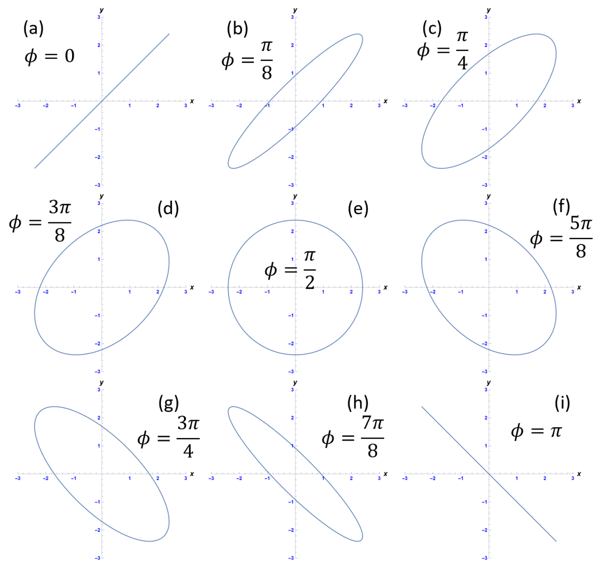
So far, the specific case of 1:1 Lissajous figures have been described. The ratio, 1:1, pertains to the coefficients of in and in Eq. (50). It is evident that , so Figure 1 shows the "one-to-one" ratio Lissajous curves for various values of . The general Lissajous curve can be described using frequencies of the ratio , where and are coprime numbers. The angular frequencies are now unique to each parametric equation; and .
| (54) | ||||
where the ratio simplifies to . In terms of and , Eq. (54) is
| (55) | ||||
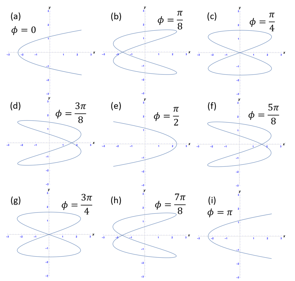
Fig. 2 shows the trajectory of the 1:2 Lissajous figure, on the range of phase, . Unlike the Lissajous ellipse, the 1:2 figure completes one full period on the same phase range. A characteristic feature of Lissajous figures is the connection between and and the number of extrema on the and axes. Fig. 1 has and one extreme point on both the and axes. Fig. 2 has and , and two extrema on the axis and one extreme on the axis. Therefore, there are extrema on the axis and extrema on the axis for a Lissajous figure.
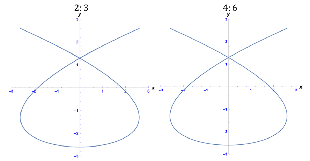
Another essential characteristic is when and are no longer coprime, i.e. , . This is the case in which there are higher harmonic frequencies. When plotted, the ratio between the frequencies simplifies to the ratio of the corresponding coprime case, but now the frequency of the higher harmonic oscillator is times faster, accounting for the increased mechanical energy in the system. This can be seen mathematically,
| (56) | ||||
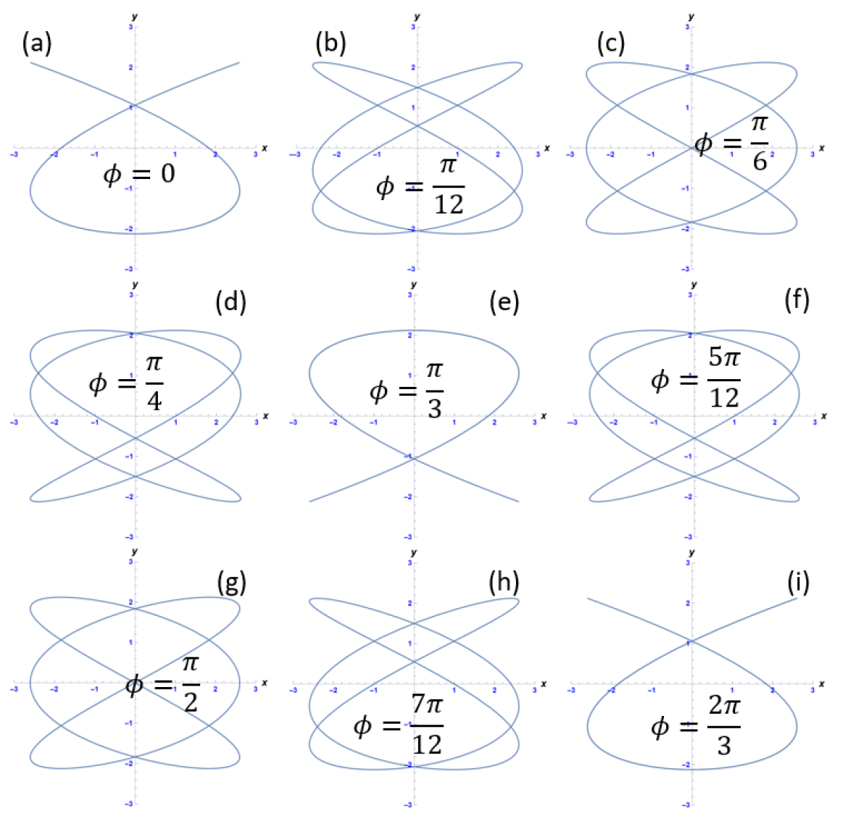
Figure 4 shows that the 4:6 and 2:3 Lissajous figures follow the same paths at the same values. In a sense, in the 4:6 Lissajous figure, there is two extrema on the axis and three extrema on the axis, but in another sense, in the same time interval, the 4:6 figure will hit every point the 2:3 figure hits, twice. The fact that evaluating the simplified fraction of applies to all possible frequency ratios. This is mentioned as a comparison to the striking difference in the quantum mechanical case presented later, where a non-coprime Lissajous ratio, , is evidence of a coherent superposition of various wavefunctions. One full phase period of a Lissajous figure, where the phase is with , is completed in the range . This can be seen from the fact that the 1:1 Lissajous figure completes its cycle on , the 1:2 Lissajous figure on , and the 2:3 Lissajous figure on .
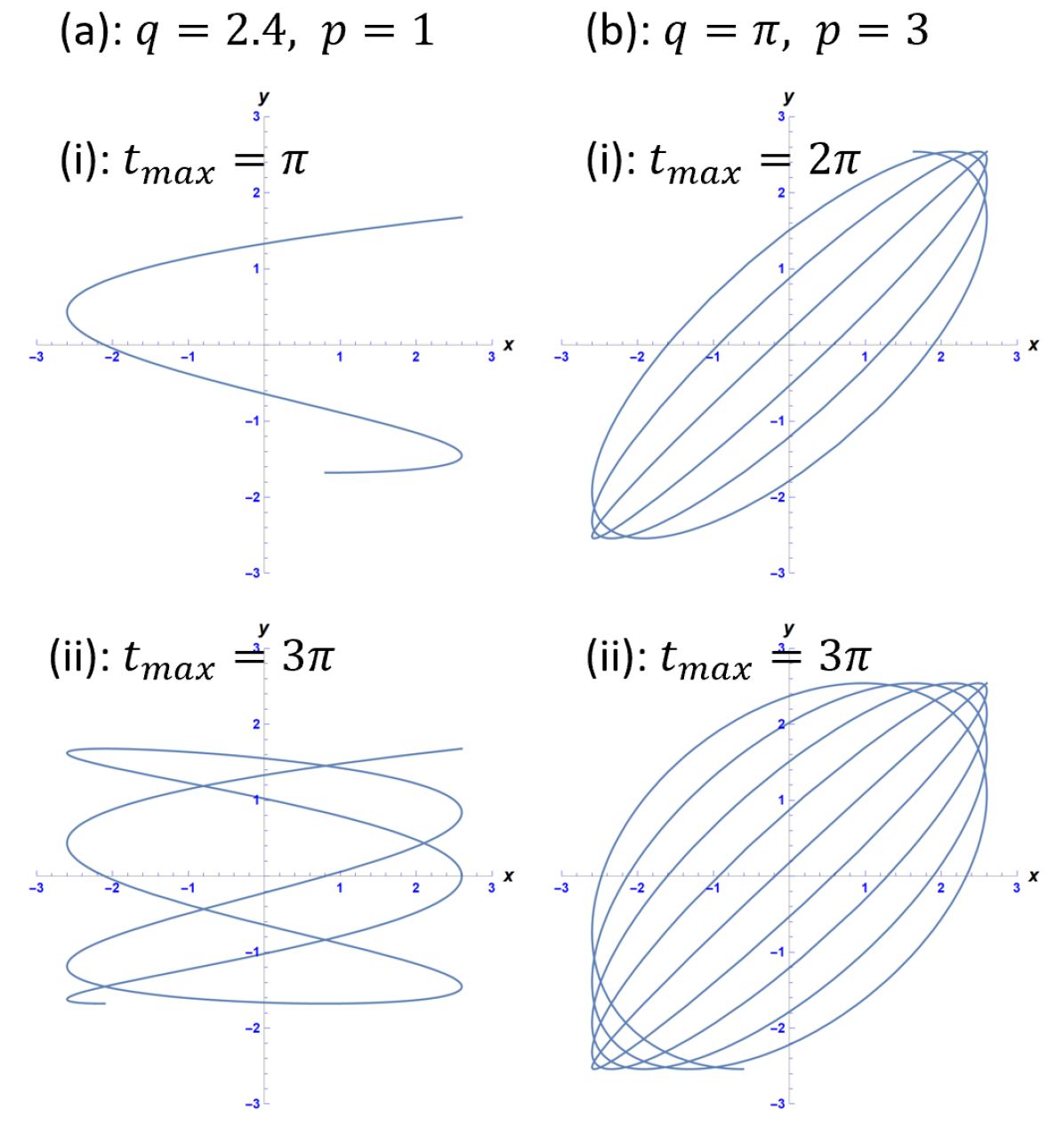
Thus far, all of the figures shown have been closed curves. A Lissajous figure is always a closed curve due to the ratio being a rational fraction. If is a rational fraction, then and are said to be commensurable. If is not a rational fraction, and are non-commensurable, and the parametric equations yield an open curves, and they are not Lissajous figures. These figures don’t travel along the same shape periodically; instead, their paths decay in a certain way related to how close the ratio, , is to a rational number. In other words, elements of Lissajous figures can be seen in open curves with similar ratios. Fig. (5) shows two examples of open curves; (a) and (b). Fig. (5)(a)(i) has a maximum time of and the shape of the 1:2 Lissajous figure (with zero phase) is traced once. The figure can be seen not staying on the 1:2 trajectory. Fig. (5)(a)(ii) has a maximum time of , and now another 1:2 figure can be seen, this time with a phase close to . This makes sense since the closest commensurate ratio to this is 1:2. Fig. (5)(b)(i-ii) have maximum times of and respectively. We see that these "cycle" through different 1:1 Lissajous figures (ellipses), which agrees with the fact that the :3 ratio is close to 1:1.
3 Quantum Lissajous Figures Via Projection
The main goal of this section is to work our way into the principal results of this research, Quantum Lissajous figures by way of projecting a degenerate subspace of the 2DHO onto a two-mode coherent state. This is not just a jump from classical Lissajous figures to quantum Lissajous figures, but rather, a journey through the history of quantum mechanics that connects to classical concepts in more than one way. A logical first step is to assume that a 2-D quantum harmonic oscillator with commensurate frequencies will exhibit properties of Lissajous figures, as the 2-D classical harmonic oscillator does, but this is not all that is needed. We start by quantizing the Hamiltonian function from section 2 by way of the Dirac prescription. Next, we introduce key concepts of quantum mechanics, like number (Fock) states and ordinary coherent (Glauber) states. Then, the description of a semi-classical Lissajous state is given. Finally, we wrap this section up by describing our derivation of fully quantum Lissajous states, via projection.
3.1 Quantum Mechanical Formulation of the 2DHO
3.1.1 Dirac Prescription
The first step to bringing this formalism to Quantum Mechanics is to generalize the Poisson Bracket. The generalization of the Poisson Bracket allows for the quantization of variables, such as the position, momentum, and the Hamiltonian. Specifically, we are working towards the raising and lowering operators, and . Dirac’s prescription states that the Poisson bracket is simply the quantum commutator divided by [6]. We define a quantum operator that corresponds to the classical
| (57) | ||||
where this substitution applies for all variables that would be inside the bracket. The commutator goes as
| (58) | ||||
Eq. (57) allows for the retrieval of the Heisenberg equation by way of Hamilton’s equation in terms of the Poisson bracket, Eq. (11). Applying the Dirac prescription to Eq. (11), and assuming the function is an observable, it becomes an operator:
| (59) | ||||
The Heisenberg equation determines the time dependence of an observable[9]. This is appropriately named due to the fact that time dependent operators is characteristic of the Heisenberg Picture of Quantum Mechanics[4]. We know that , so plugging this into the Dirac prescription gives
| (60) | ||||
which shows that the commutator of the operator is
| (61) | ||||
To get to that Bosonic ladder operators, , a rescaling of is required. Letting ,
| (62) | ||||
For , we define a quantum operator that is equal to , and come to
| (63) | ||||
We can apply the Dirac prescription on the canonical coordinates as well
| (64) | ||||
which yields the canonical commutation relation
| (65) | ||||
Note that the on the right hand side of Eqs. (64) and (65) is the imaginary number, the subscript is an index where . For the and coordinates,
| (66) | ||||
The Dirac prescription is more straight forward for the canonical and normal coordinates, they all become quantum operators. From Eq. (32) we get
| (67) | ||||
and again, rescaling using and
| (68) | ||||
Now with the inclusion of , these operators are inherently quantum mechanical. The presence of is a sign of a quantum mechanical system, due to the fact that is a proportionality constant between a photon’s energy and angular frequency, , and between a photon’s momentum and angular wave number, [7]. The position and momentum operators can be found from Eq. (68)
| (69) | ||||
| (70) | ||||
The Hamiltonian function, Eq. (23), in operator form is
| (71) | ||||
One might assume that the quantum Hamiltonian in terms of Ladder operators will be of the same form as Eq. (33), but this is not the case. The operators and do not commute, and so the cross-terms of do not add to zero:
| (72) | ||||
To get rid of the cross-terms, the Hermitian conjugate of , , should be looked at:
| (74) | ||||
Multiplying Eq. (74) by gives
| (75) | ||||
This is the component of the Hamiltonian operator, Eq. (71). Recell Eq. (62), expanding the commutator bracket
and isolating gives
Plugging this into Eq. (75)
| (76) | ||||
The component of the Hamiltonian is found by analogy
| (77) | ||||
The total Hamiltonian, in terms of and is then
| (79) | ||||
3.1.2 Number States (Fock States)
The raising and lowering operators, and , where , are named as such due to the result of when they’re applied to the Number states, ,
| (80) | ||||
| (81) | ||||
If we apply to Eq. (80), the result is
| (82) | ||||
This combination of operators, , is the same form as what appears in the quantum harmonic oscillator’s Hamiltonian. It is called the Number operator
| (83) | ||||
Eq. (82) shows that the number state is an eigenstate of the number operator. Explicitly, the eigenvalue equation is
| (84) | ||||
where is a nonnegative integer, i.e. . Number states can be constructed from the ground state,
| (85) | ||||
It is useful to know the commutation relation between and
| (86) | ||||
and between and
| (87) | ||||
Consider the 1-dimensional Hamiltonian given by Eq. (76). It can be rewritten in terms of the number operator
| (88) |
By inspection, we see that is also an eigenstate of Eq. (88)
| (89) | ||||
with an eigenvalue
| (90) | ||||
The wavefunction of the Fock state is found by projection of the configuration space state
| (91) |
where
| (92) |
and is the Hermite polynomial. Back to the 2-dimensional case, we choose the convention where the operators are applied to the number state, and the operators are applied to the number state. Eq. (79) in terms of number operators becomes
| (93) | ||||
3.1.3 Coherent States of the Free Field (Glauber States)
As per the theme of this study, we wish to find classical-like behavior in the quantum regime. The Glauber states are minimum uncertainty states, which already makes them more classical than other states, but this fact comes to front explicitly in Heisenberg’s uncertainty principle, in which the canonical position and momentum operators are directly involved[10]. The coherent state is an eigenstate of the lowering operator, such that,
| (94) | ||||
where is a complex number. The coherent state in the number state basis is given as[8]
| (95) | ||||
The general uncertainty principle applies to three observables that satisfy the commutation relation
then the uncertainty for some quantum state is
| (96) | ||||
where is the variance of an operator
and the expectation value of the variances works out as such:
| (97) | ||||
To retrieve Heisenberg’s uncertainty principle, we use the canonical commutation relation given by Eq. (65), where , , and
| (98) | ||||
From here, we consider the direction for continuity, and it is easy to show that for the coherent state , the Heisenberg uncertainty principle is minimized,
| (99) | ||||
verifying that the coherent state is a minimum uncertainty state. We can build coherent states from the number state basis, with the introduction of the displacement operator,
| (100) | ||||
The displacement operator is a unitary operator, i.e. the multiplication of itself and its Hermitian conjugate yields the identity operator,
| (101) | ||||
It is also worth noting that
| (102) | ||||
and also
| (103) | ||||
The properties in Eqs. (102) and (103) are found with the use of the Baker-Campbell-Hausdorff lemma[8]; for two arbitrary operators and ,
| (104) | ||||
This is not to be confused with the Baker-Campbell-Hausdorff Theorem[8]; for two operators and that do not commute, i.e. , if
then
| (105) | ||||
The Baker-Campbell-Hausdorff Theorem allows for Eq. (100) to be expressed in its normally ordered form[10],
| (106) | ||||
The normally ordered form of the displacement operator is a tool used to reach Eq. (95). If the normally ordered displacement operator is applied to the ground state , we retrieve the coherent state
| (107) | ||||
3.2 Semi-classical Dynamics
We have discussed the properties of the single-mode ordinary coherent states. To argue for the possibility of quantum Lissajous figures, it is only natural to begin with a two-mode ordinary coherent state since ordinary coherent states are minimum uncertainty states and classical Lissajous figures arise from a 2-dimensional system of orthogonal harmonic oscillators.
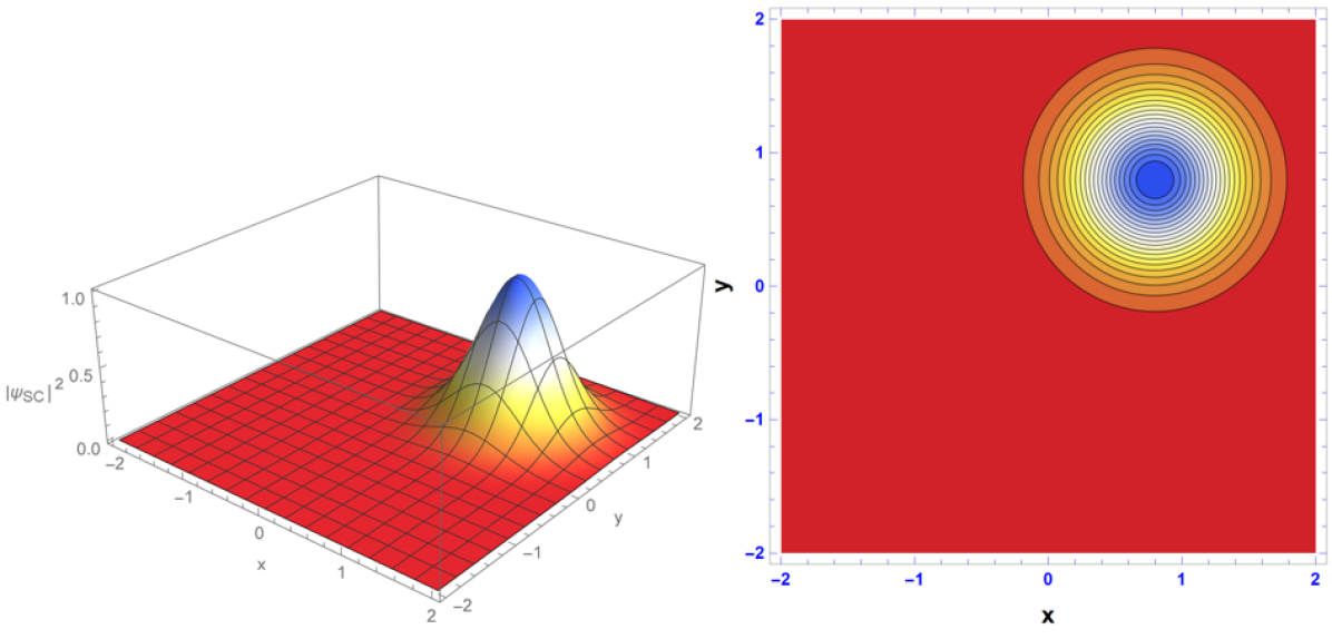
| (108) | ||||
Eq. (108) as is, produces a probability density function that is a Gaussian displaced from the origin of configuration space by in the -direction and in the -direction. Therefore, it does not immediately give indication of being related to Lissajous figures.
Where it becomes related, is when the time evolution operator is applied. Working in 1-dimension for simplicity, the time evolution operator is given by
| (109) | ||||
and like Eq. (100), it is unitary. is given by Eq. (76). Applying the time evolution operator to the ordinary coherent state gives
| (110) | ||||
where the complex phase out front can be neglected as it does not contribute to normalization. It is clear that this state is not stationary, i.e. the probability density is time-dependent. Moving into two dimensions, the 2-dimensional time evolution operator is given as
| (111) | ||||
and when applied to the two-mode coherent state yields
| (112) | ||||
which is simply the multiplication of two single-mode coherent states. The configuration space wavefunction, , is given by
| (113) | ||||
where is given by Eq. (91), and by analogy is
| (114) |
with
| (115) |
For the rest of this study we set and such that and . An alternative form of Eq. (113) can be found by employing the use of the generating function of Hermite polynomials[arfken ref]. That is,
| (116) |
The time-dependent two-mode coherent state is then
| (117) | ||||
To begin, we consider the isotropic case where . Eq. (113) becomes
| (118) | ||||
where the single mode wavefunctions are
| (119) |
and
| (120) |
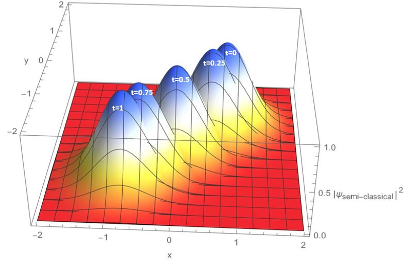
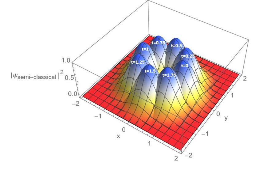
Plotting the probability density
| (121) | ||||
we expect the average value of the Gaussian wave packet to move like a classical particle, at the same velocity of that particle[4]. This is Ehrenfest’s Theorem, which says that quantum mechanical expectation values follow the classical laws of motion[5]. We have already shown these states to be non-stationary, so there mustn’t be a steady current density, . According to the continuity equation
| (122) |
the divergence of the probability current density can only be zero if the probability density is time-independent, but these states are time-dependent. In order to satisfy the continuity equation, the divergence of the current density must offset the non-zero value of the partial derivative of with respect to time. Having a non-steady current makes perfect sense in a classical setting, a classical oscillator would have acceleration, breaking the "steady flow" of velocity.
The verification of Ehrenfest’s Theorem does not stop at Fig. 7. All possible phase differences between and will exhibit this behavior, as well as other coprime ratios of frequency. These are what are known as semi-classical Lissajous states, coming from the fact that we are dealing with the most classical of quantum states and that probability density mimics the shape of Lissajous figures through time. The quantum Lissajous figures via projection, proposed below, encode the Lissajous figures in an even more fundamental way while being stationary and having a steady current flow. Before we reach that section of this section, we will continue with more examples of these semi-classical states. Next is to examine some semi-classical examples where the phase difference between the complex amplitudes is non-zero.
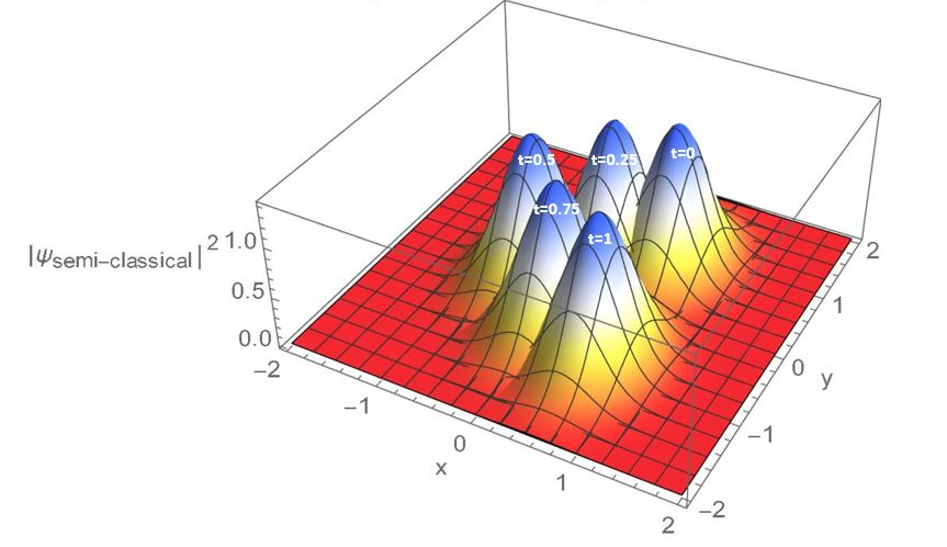
Now we consider and , where and are integers that form a commensurate frequency ratio between and . Eq. (113) becomes
| (123) | ||||
where the single-mode harmonic oscillator wavefunctions are
| (124) |
and
| (125) |
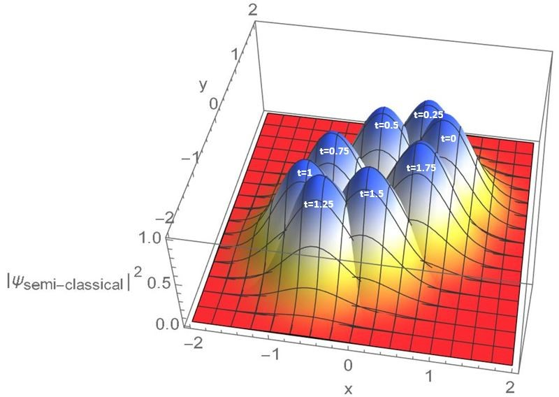
Plotting the probability density,
| (126) | ||||
we expect this to act exactly like the isotropic case, in that the centroid of the Gaussian travels along the path of corresponding classical Lissajous figures, but now for ratios that are not 1:1. Therefore, Ehrenfest’s Theorem is doubly justified in the cases of semi-classical Lissajous states.
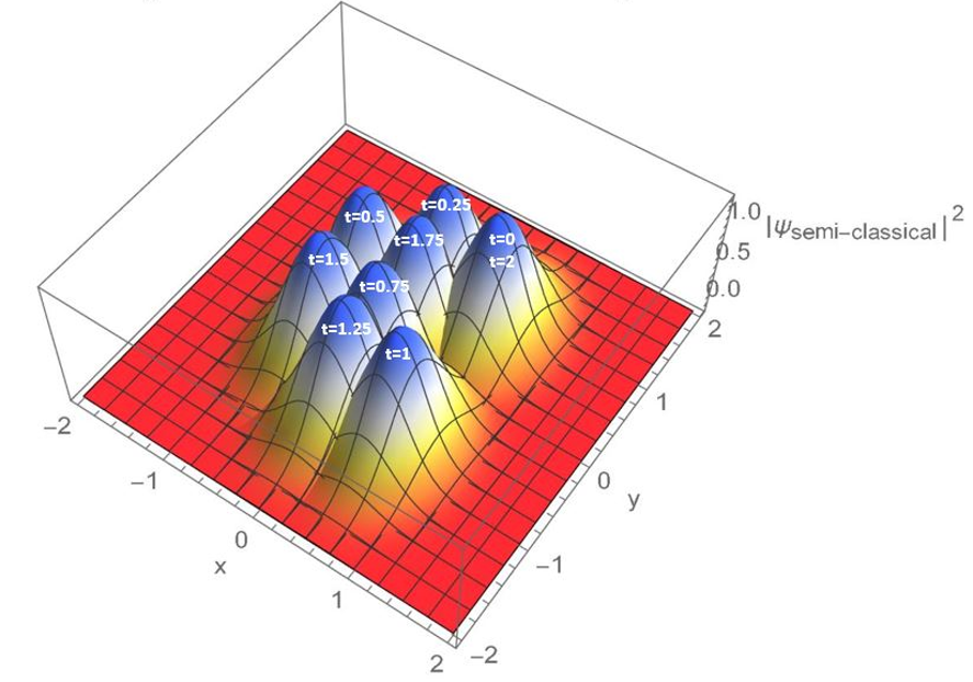
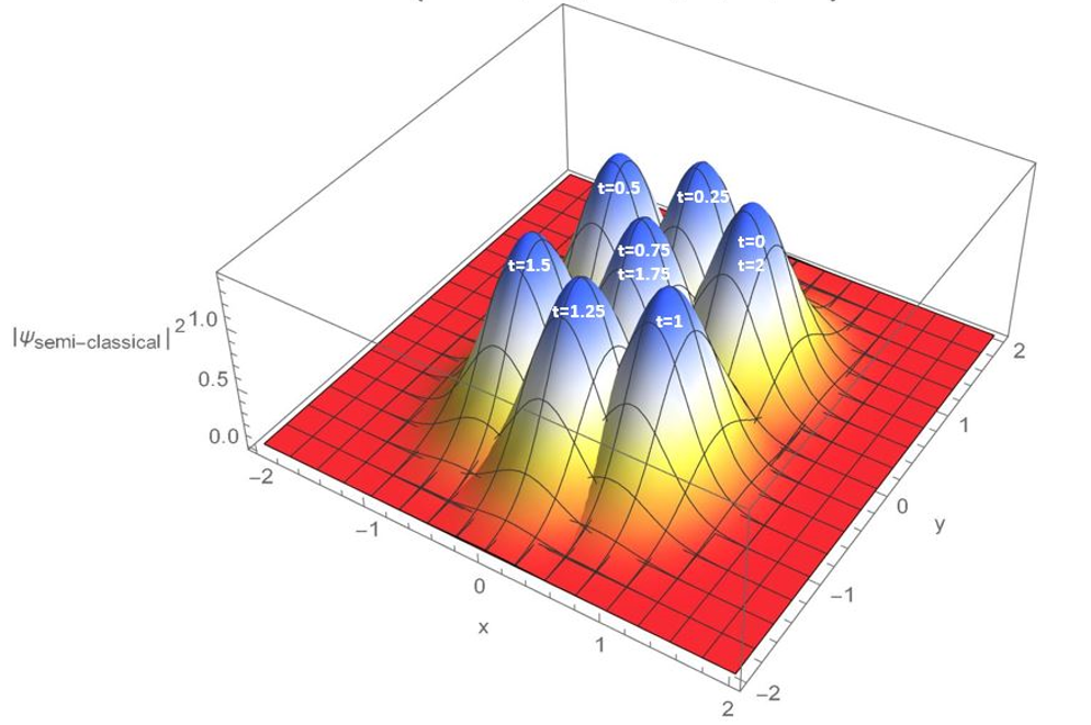
Once again, it is of much importance to note that according to Ehrenfest’s Theorem, the centroid of the probability density holds its Gaussian shape while evolving along the trajectory of classical Lissajous curves, as seen in Figs. 7-12. There is an even more striking form of Lissajous states in quantum mechanics: stationary states with steady current densities. These states will encode the Lissajous trajectories in a more fundamental and quantum mechanical fashion.
3.3 Quantum Lissajous Figures-Fundamental Cases
This section contains the analysis of states that we have shown to be inherently quantum mechanical analogs to classical Lissajous figures. Unlike the previously mentioned semi-classical Lissajous states, these states encode whole classical Lissajous figures in a corresponding probability density. Time evolution is trivial when applying to a degenerate subspace, so the quantum Lissajous states are stationary with steady current density. Two separate classes of quantum Lissajous states will be analyzed: "fundamental" and "higher harmonic" quantum Lissajous states. The fundamental case’s constraint is that the frequencies must be coprime, whereas the higher harmonic case is categorized by having non-coprime, but still commensurate frequencies. Some examples of fundamental cases are , , and ; and higher harmonic cases include, but are not limited to, , , and . Recall, when reviewing the classical Lissajous figures, cases with higher harmonic-like ratios simplified to the coprime cases and only rescaled the size of the figures based on increased mechanical energy. For quantum Lissajous states, this is strikingly different. The higher harmonic quantum Lissajous figures do not simplify to the corresponding fundamental quantum Lissajous figure, they become linear superpositions of fundamental quantum Lissajous figures with certain complex phases.
Starting back up with with Eq. (93), this Hamiltonian acts on a composite Fock state, .
| (127) | ||||
The Fock state remains unchanged after the operation of the Hamiltonian, and we retrieve the energy eigenvalue,
| (128) | ||||
3.3.1 Fundamental Isotropic Case
The fundamental isotropic quantum Lissajous figure is categorized by its one-to-one frequency ratio, . Applying this to Eq. (79) yields the simplest form of the 2DHO Hamiltonian,
| (129) |
The fundamental isotropic Hamiltonian has SU(2) as its dynamical symmetry (degeneracy) group. Through the introduction of the Schwinger Realization[13],
| (130) |
and
| (131) |
we can express Eq. (129) in terms of angular momentum operators. Eqs. (130) and (131) obey the commutation relation
| (132) |
We also introduce the operator
| (134) |
An important object in Lie algebra, and specifically in the realm of angular momentum operators is the Casimir operator[14]. The Casimir operator for this algebra is
| (135) |
which means that can be considered the Casimir operator. We can rewrite the fundamental isotropic Hamiltonian, Eq. (129) as
| (136) |
Equation (136) shows that the Hamiltonian is a function of the Casimir operator, which is a characteristic feature of degeneracy groups. The ability for the Hamiltonian to be expressed in terms of shows the rotational symmetry of the isotropic oscillator. For a system of quanta, the corresponding degenerate eigenstates are for , , and where
| (137) |
The degenerate states defined in equation (137) satisfy the eigenvalue equation
| (138) |
with a degeneracy of , owing to the fact that there are states of the form for .
It is well known that the SU(2) coherent states[10], by analogy with ordinary coherent states, are formed by applying a rotation operator on the ground state in the angular momentum basis, where the rotation operator takes the place of the displacement operator in the ordinary coherent state case. The rotation operator
| (139) |
where and , is the one appropriate for rotating the spin-down state into an SU(2) coherent state localized on the Bloch sphere at azimuthal angle, , and latitude angle, , as measured relative to the south pole.
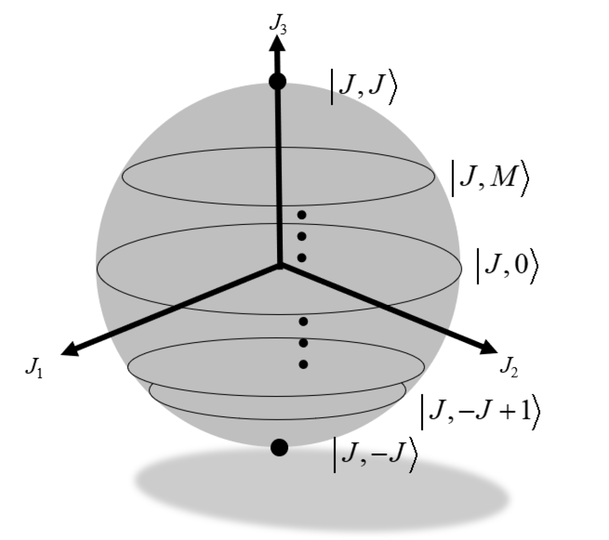
The Bloch sphere is a 2-dimensional surface embedded in a 3-dimensional angular momentum space that gives a representation of angular momentum states. In particular, regions on the Bloch sphere represent states in a spin- system. For example, in Fig. 13, we show several of the eigenstates of in the basis in which the operator is diagonal. In general, states on the Bloch sphere correspond to extended regions owing to the uncertainty principle for angular momentum operators, which is why states of well-defined are represented by latitude lines on the Bloch sphere. On such a line, the eigenvalue of is well-defined, but the values of and are distributed randomly around the latitude line. The spin-up and spin-down states are exceptional in that they correspond to points on the Bloch sphere, which, strictly speaking, seem to violate the uncertainty principle. However, these points should be thought of as limiting cases of latitude lines with uncertain and .
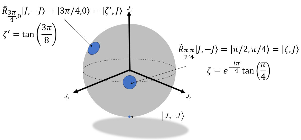
In Fig. 14, we represent the action of the rotation operator, Eq. (139), on the ground state, , to form an SU(2) coherent state localized around the desired location on the Bloch sphere.
We now use the idea of rotation on the Bloch sphere and the connection between the angular momentum basis states and the two-mode Fock states within a degenerate subspace of the 2DHO to illustrate the identification of the isotropic quantum Lissajous states with the SU(2) coherent states. The second equality in Eq. (139) is the normally ordered form of the rotation operator and is found using the disentangling theorem for angular momentum operators[11]. The Schwinger Realization[13] allows us to treat this angular momentum system as two uncoupled quantum harmonic oscillators[4] where the number of quanta is equal to double the maximum value of angular momentum, . Since , the oscillator initially holds all quanta. Applying the rotation operator on the state ,
| (140) |
which shows that the SU(2) coherent states are formed over the degenerate states of the two-mode harmonic oscillator.
We now introduce our formulation of the quantum Lissajous states for the isotropic 2DHO by considering the projection of the ordinary two-mode coherent state onto a degenerate subspace of the system, thereby, guaranteeing the result is a stationary state. The projection operator onto the degenerate subspace has the form, for a given of
| (142) |
which when normalized becomes,
| (143) |
where . Comparing Eq. (143) with Eq. (140), we see that the projected state is indeed an SU(2) coherent state. If we consider this state on the Bloch sphere, we can draw the correspondences that , the relative phase between and in the projected state is identified with the azimuthal angle appropriate to the Bloch sphere representation of this state. Further, the ratio, is identified with . It is important to keep in mind that these analogies, while compelling, are just analogies. The Hilbert space represented by the Bloch sphere is different than the Hilbert space of the 2DHO. We employ this analogy as a means of understanding the SU(2) structure of the projected states of the isotropic 2DHO, but, the eventual connection with Lissajous figures occurs the configuration space of the 2DHO, not on the Bloch sphere.
Applying the time evolution operator to Eq. (143), it is clear that the time evolution behaves like a global phase
| (144) |
thus, the probability density is time-independent. Eq. (143) is in agreement with Eq. (140), successfully reaching the SU(2) coherent state via projection.
To see the connection with Lissajous figures, we must study the configuration space probability density for projected states. To do this we must form the configuration space wavefunction. The wavefunction associated with equation (143) is found by projection onto configuration space, :
| (145) |
where the 1-dimensional wavefunctions are separable and given by,
| (146) |
and
| (147) |
These are the usual wavefunctions of a 1DHO, which involve Gaussian factors and Hermite polynomials, and . The probability density associated with equation (145) is
| (148) | ||||
As we will demonstrate in section 4, where we present our major results, the support of the distribution given in Eq. (148) lies along the classical Lissajous figure for the isotropic 2DHO. It is for this reason that we describe our projected states as "quantum Lissajous states."
Throughout this literature, we assume to be real and take so that with . This assumption does not restrict the cases which can be studied since the phase is transferable to either complex amplitude. The phase, , and amplitude, , affect the eccentricity and orientation of the Lissajous figure along which a quantum Lissajous state is localized. The quantum Lissajous state is a stationary state, which is completely due to the projection onto the degenerate states, so it will no longer move in time. Instead, the whole probability density will localize along the classical Lissajous ellipse. Graphical evidence of these characteristics will be shown in the next section.
3.3.2 Fundamental Anisotropic Case
The role of projection onto degenerate states becomes much more significant for the fundamental anisotropic oscillator. The anisotropic Hamiltonian is given by Eq. (79)
| (149) | ||||
With the introduction of the factors of and , we can still use the Schwinger realization[13] to represent the Hamiltonian in terms of angular momentum operators, but we cannot represent the Hamiltonian in terms of only the Casimir operator,
| (150) |
As a result, the anisotropic Hamiltonian no longer commutes with the rotation operator that generates an SU(2) coherent state on the Bloch sphere, breaking the rotational symmetry of the system. Therefore, appealing to the correspondence we developed above between SU(2) coherent states on the Bloch sphere and the projected states of the 2DHO, we expect that the quantum Lissajous states for the anisotropic oscillator are not SU(2) coherent states. In other words, because the anisotropic Hamiltonian doesnt commute with the rotation operator, Eq. (139), there is no way to start with the ground state and rotate into an anisotropic quantum Lissajous state while remaining in the same degenerate subspace. The derivations that follow will mirror those for the fundamental isotropic 2DHO.
The Hamiltonian for the anisotropic oscillator is given by Eq. (149), where and are coprime numbers, and and are commensurate frequencies. The degenerate eigenstates of the Hamiltonian, Eq. (149), are given by , for and , and where
| (151) |
The fundamental anisotropic Hamiltonian satisfies its own eigenvalue equation,
| (152) |
with an eigenvalue of , with a degeneracy of . This is a result of accidental degeneracy since there is no rotational symmetry. The projection operator for the fundamental anisotropic oscillator is,
| (153) |
Performing the projection on and disregarding global factors,
| (154) |
and when normalized, becomes
| (155) |
where and the normalization constant is
| (156) |
Eq. (155) is no longer an SU(2) coherent state, as expected. Although the degeneracy is still , characteristic of SU(2), now the rotational symmetry of the system has been broken. This is evident from the fact that the coefficient inside the summation cannot be simplified to the binomial coefficient, as would have to be the case for an SU(2) coherent state. Consequently, in the normalization constant yields the summation recognized as the binomial theorem and leads to the isotropic oscillator’s normalization constant, . Some authors have attempted to formulate "generalized SU(2) coherent states", but we find this to be inaccurate[22, 24, 23, 12]. It is true that setting in Eq. (155) gives back the SU(2) coherent state, but, Eq. (155) is not a "generalized SU(2) coherent state" due to the lack of rotational symmetry; is the characteristic feature that preserves rotational symmetry to the isotropic oscillator.
Applying the time evolution operator to Eq. (155), the time evolution behaves like a global phase
| (157) |
thus, these are stationary states with a steady probability current density. The wavefunction associated with Eq. (155) is again found by projection onto configuration space, :
| (158) |
where the 1-dimensional wavefunctions are still separable, but more complicated:
| (159) |
and,
| (160) |
It can be seen that the anisotropic 1-D wavefunctions hold the same form as their isotropic counterparts, but now with factors of and that change the proportionality of the equations. The current density for Eq. (158) is given by
| (161) |
We keep the convention of holding to be real and taking to be complex, . The anisotropic complex amplitude is then . Eq. (161) produces patterns localized along classical Lissajous figures of commensurate frequency ratios. The phase, , now changes the shape of the Lissajous curve, i.e. the path that is traced. Just like classical Lissajous curves, the phase cycles through different shapes that Lissajous figures evolve in and out of. The quantity changes the orientation of the figures in configuration space. Graphical examples will be shown in section 4 to show the roles of phase and orientation.
3.4 Quantum Lissajous Figures-Higher Harmonic Cases
The theory in section 3.3 refer to states having frequency ratios where and are coprime numbers. We refer to these states as fundamental quantum Lissajous states of the isotropic and anisotropic 2DHO. We refer to frequency ratios that are not coprime as higher harmonic quantum Lissajous states. Classically, there is no unique higher harmonic Lissajous curve, as the frequency ratio reduces to its lowest terms, or in other words, reduces to the fundamental case. This can be seen in Fig. (4). There is no visual change to the higher harmonic classical figures, but there is an increase in the total mechanical energy of the system. The quantum mechanical higher harmonic cases do not reduce as their classical counterparts do, but they can be explained in terms of the fundamental quantum Lissajous states.
3.4.1 Isotropic Higher Harmonic Quantum Lissajous State
Recall that we’ve shown the fundamental isotropic 2HDO states to be an SU(2) coherent state[10]. Using Eqns. (155) and (156) with ,
| (162) |
where and the normalization constant is
| (163) |
it is easy to show that the mth harmonic isotropic quantum Lissajous state can be written as a linear superposition of fundamental isotropic quantum Lissajous states having; quanta, frequencies that are times the frequency of higher harmonic state, , and complex amplitudes that are weighted by factors that are the distinct the mth roots of unity,
| (164) |
The wavefunction corresponding to Eq. (164) accounts for the quanta, frequency characteristics and the roots of unity of this superposition
| (165) |
The normalization constant of the isotropic higher harmonic 2DHO turns out to be the ratio of two normalization constants, both of which can be found using Eq. (156), and multiplied by ,
| (166) |
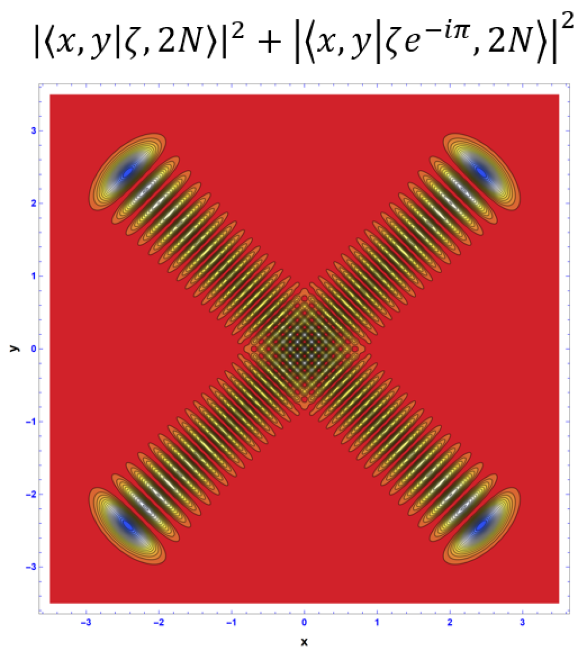
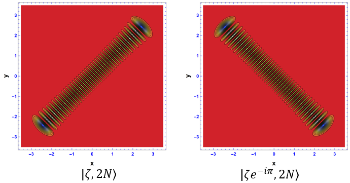
The constant in the numerator is Eq. (156) with and quanta, while the one in the denominator is Eq. (156) with and quanta. It is obvious that the normalization constant on the left hand side of Eq. (164) is , thus we see it included on the right hand side. is included in the denominator to eliminate the normalization constants of the states in the superposition. The states given by Eq. (164) are generalizations of the SU(2) cat states, which turn out to be the isotropic higher harmonic quantum Lissajous states for [15], and also generalizations of the SU(2) compass states, which are the isotropic higher harmonic quantum Lissajous states for [16]. Once again, the isotropic higher harmonic quantum Lissajous states are superpositions of SU(2) coherent states, which in and of itself is non-classical. The concept of superposition gives rise to quantum interference, which will be shown graphically in section 4. The interference terms can be seen by writing out the probability density
| (167) |
The summation with are the individual probability densities in the superposition and the summation with gives rise to the quantum interference between the wavefunctions in the superposition. Each wavefunction interferes with all the others separately.
3.4.2 Anisotropic Higher Harmonic Quantum Lissajous State
Now consider the anisotropic higher harmonic quantum Lissajous states , for which . Interpolating on the isotropic case, one can figure that the superposition now involves fundamental anisotropic quantum Lissajous states, Eq. (155), instead of the fundamental isotropic states. Let and be coprime numbers where and , which leads to . Using Eq. (155), it is easy to show that the mth harmonic anisotropic quantum Lissajous state can be written as a linear superposition of fundamental anisotropic quantum Lissajous states having; quanta, frequencies that are times the frequency of higher harmonic state, , and complex amplitudes that are weighted by factors that are the distinct the mth roots of unity,
| (168) |
with the wavefunction
| (169) |
where, similar to the isotropic higher harmonic 2DHO, the normalization constant is the ratio of two normalization constants of Eq. (156),
| (170) |
The relationship between and is simply . Eq. (168) is similar to Eq. (164) in the sense that the higher harmonic state can be decomposed as linear superpositions of fundamental quantum Lissajous states with phases corresponding to th roots-of-unity, but the fundamental states on the right-hand-side of Eq. (168), , are no longer SU(2) coherent states. It is true that for a state of quanta, there is an -fold degeneracy which is characteristic of SU(2), but in the anistropic case, the rotational symmetry is broken in contrast with the case of the isotropic 2DHO. For Eq. (168) becomes Eq. (164). The probability density of the anisotropic higher harmonic quantum Lissajous state can also be written in such a way to separate interference terms from the terms that encompass the individual probability densities, refer to Eq. (167).
3.5 Probability Current Density for the Quantum Lissajous States
The probability current density is a vector quantity that describes the flow of probability. It can be thought of in the context of hydrodynamics (electromagnetism) as the flow of fluid (charge)[4]. The probability current density along with the probability density, due to local conservation of probability, must obey the continuity equation
| (171) |
The already discussed probability density is given by
| (172) |
and the probability current density in general is
| (173) |
To understand more about how the probability current density is characterized, consider a wavefunction of the form
where and are real numbers that are functions of space and time generally. The probability density becomes
and by using Eq. (173), the probability current density is
| (174) |
Eq. (174) tells us that the spatial variation of the phase defines the behavior of the probability current density[4]. Eqs. (144) and (157) show that the quantum Lissajous states formed via projection on their respective degenerate subspaces are stationary states; thus the probability density is time-independent, and the continuity equation for these states becomes
| (175) |
which says the current density is steady. Two distinct behaviors emerge due to Eq. (175); the current density can vanish (), or the current density can be non-zero in a way consistent with laminar flow of probability (, but ). In the case of , quantum interference is maximal, with fringes appearing in the probability density , perpendicular to the motion of the current density, called static states. In the case of , there are varying amounts of quantum interference, and representative examples will be shown of the emergence of quantum interference in section 4. A non-zero current density will require the divergence of the current to vanish to satisfy the continuity equation. These are vortex states. In section 4, graphical results will be shown, along with conceptual descriptions, to develop a connection between the nature of non-zero, steady probability current density and the emergence of quantum interference in the quantum Lissajous states for both isotropic and anisotropic oscillators and for both fundamental and higher harmonic cases.
4 Representative Examples of Principal Results
Section 4 is intended as an abridged archive of several quantum Lissajous figures illustrating the important non-classical features (quantum interference, natural emergence of roots-of-unity superpositions) and allowing for the comprehensive comparison of the fundamental cases with the corresponding classical Lissajous figures. We will present graphical results based upon numerical renderings of our analytical results from section 3 to demonstrate the important mathematical features of the quantum Lissajous figures formed via projection onto a degenerate subspace. The comparison between the quantum and classical cases (where possible) is exquisite in its accuracy, justifying the nomenclature we have chosen for the states we have studied here.
4.1 Fundamental Isotropic Quantum Lissajous State
The results presented in this section correspond to the theory developed on the fundamental isotropic quantum Lissajous states, Eq. (143), and its wavefunction, Eq. (145). The probability density is calculated using Eq. (148) and the probability current density using Eq. (173).
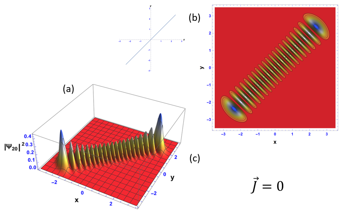
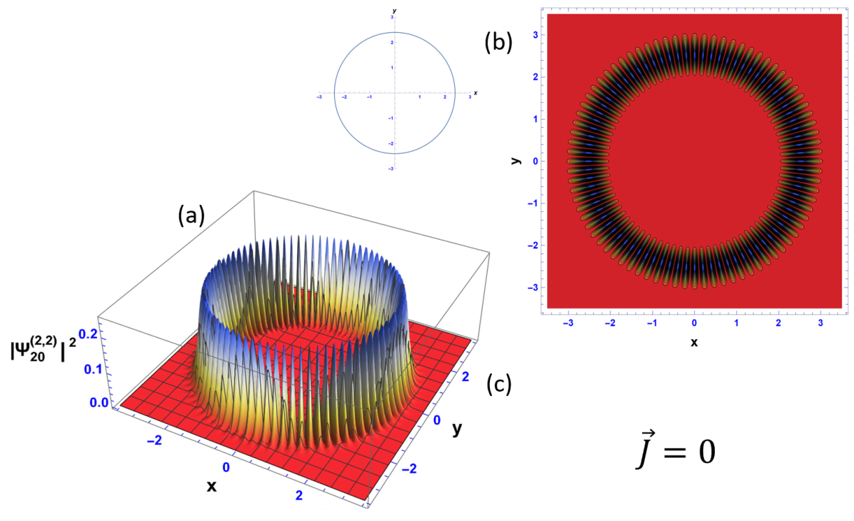
Fig. 15 presents the surface (a) and contour (b) plots of the probability density, as well as the vector (c) plot of the probability current density of the fundamental isotropic quantum Lissajous state, Eq. (145), for , complex amplitudes in phase. Just as in all other probability densities, the highest peaks are where the oscillator is most likely to be. The fringes that appear here are analogous to the patterns found in double-slit interference so we have referred to the probability peaks as "bright spots" and the minima as "dark spots". It can be seen that probability density localizes over the classical Lissajous figure for (Fig. 1(a)), which is pictured to the left of Fig. 15(b). The probability current density completely vanishes. The classical oscillator travels along the path of a Lissajous figure; in the case of the classical Lissajous figure, the oscillator travels along the path of the straight line on and temporally oscillates on that line. For the quantum oscillator, the probability density spatially oscillates along the corresponding Lissajous figure. Because the oscillation is isolated along one line, and the probability current density vanishes, the probability current must be equal and opposite so for it to cancel out and vanish. The most striking feature in this figure is the appearance of fully resolved interference fringes. As more examples are shown, it will become increasingly clearer that quantum interference fringes appear along sections of quantum Lissajous figures where the probability current is "counter-propagating" and that quantum interference fringes are maximally resolved for vanishing probability current density. Fig. 15 satisfies the continuity equation, Eq. (171), by having a vanishing probability current. Thus, this is a static quantum Lissajous state and, in fact, is the static limit of the quantum Lissajous states for the isotropic 2DHO.
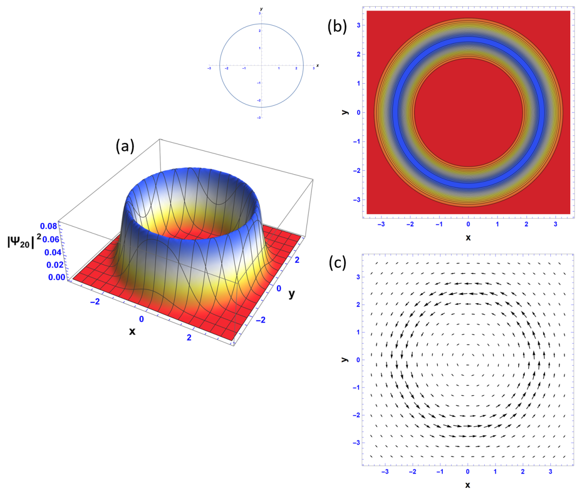
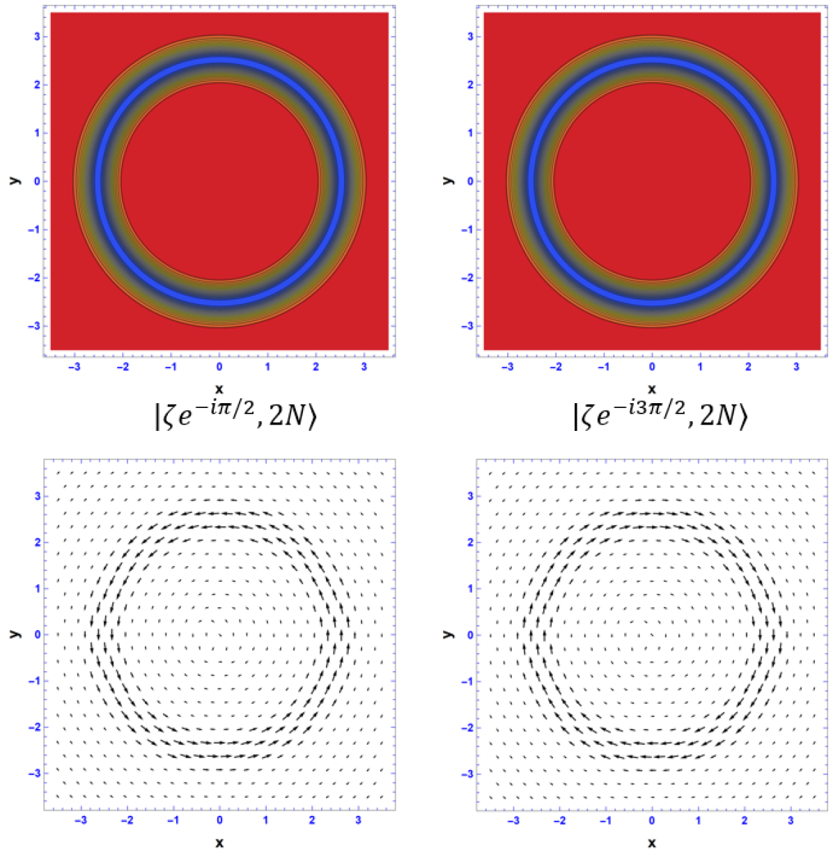
Fig. 16 presents the surface (a) and contour (b) plots of the probability density, as well as the vector (c) plot of the probability current density of the fundamental isotropic quantum Lissajous state, Eq. (145), for and , complex amplitudes in quadrature. It can be seen that probability density localizes over the classical Lissajous figure for , which is pictured to the left of Fig. 16(b). The probability current density is steady and flows in the counter-clockwise (CCW) direction, which matches the classical oscillator of the same phase. There are smooth and monotonic spatial variations in probability owing to the lack of quantum interference fringes. The CCW propagating current by itself is conducive to the absence of interference fringes, as there is a steady but non-zero probability current. Fig. 16 satisfies the continuity equation, Eq. (171), by having a divergenceless current density. This is easy to see in Fig. 16(c) as the current flows back into itself. This idea is analogous to magnetic fields by way of Gauss’ law for magnetism, , which states that magnetic monopoles do not exist because the magnetic field is divergenceless[17]. This is the vortex limit of the quantum Lissajous states for the isotropic 2DHO. Notice that from Fig. 15 to Fig. 16, the quantum interference fringes wash away. As the phase is increased from to , we expect to see the quantum interference fringes to disappear in such a way that corresponds to the absence counter-propagation of current density. Examples of the fundamental isotropic quantum Lissajous states for phases in the range are shown in Figs. 17-20, and will defend the fact that quantum Lissajous figures localize along their classical counterparts of the same phase difference, as well as depict the emergence (or disappearance) of interference fringes.
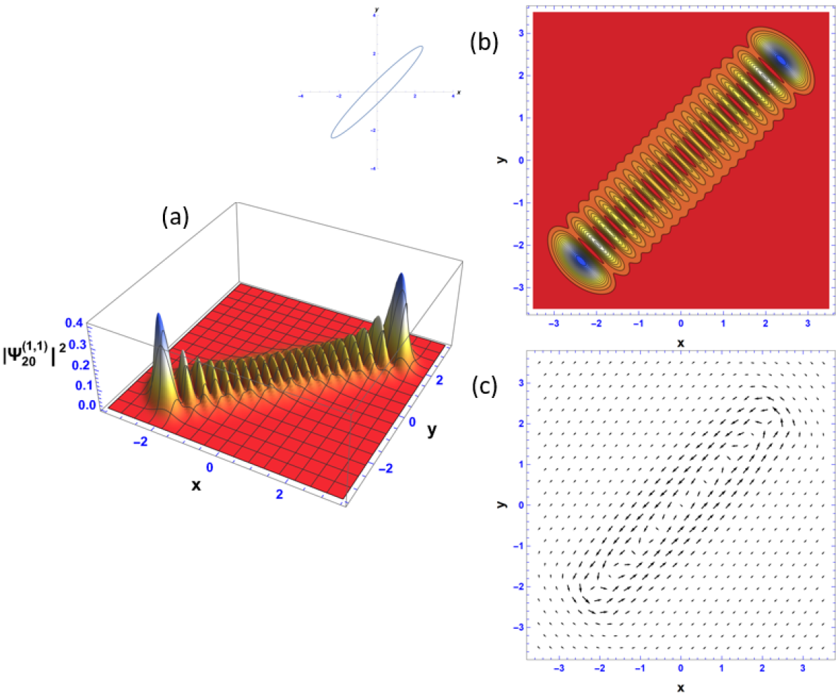
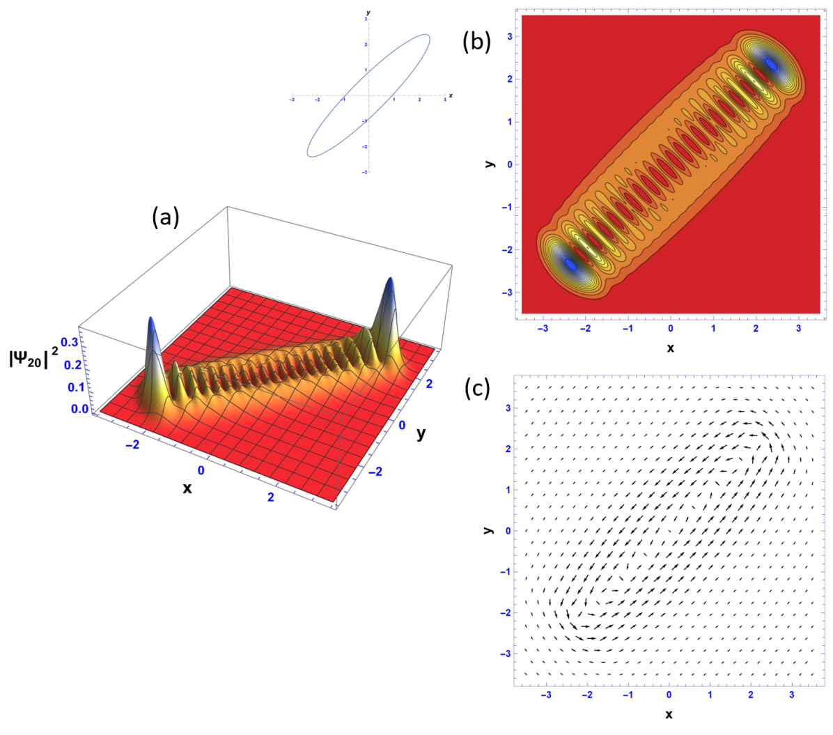

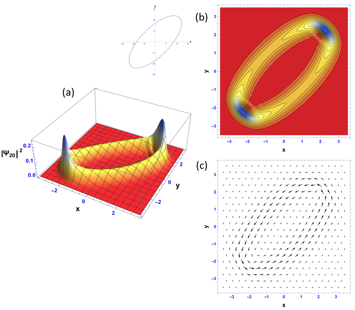
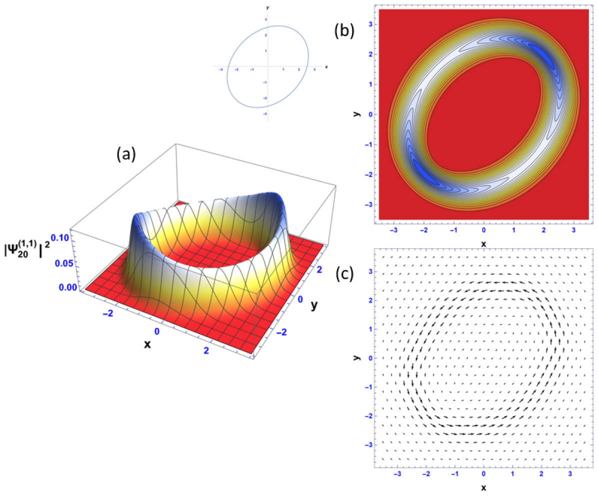
Fig. 17 presents the beginning for the transition from a line segment to an ellipse. The interference fringes are no longer fully resolved, as in Fig. 15. The probability in each fringe flows out of the bright spot and into the surrounding space, meeting the adjacent fringe’s probability "leak", which connects the fringes at their ends and encloses the dark spots. A vortex emerges in the shape of a highly eccentric ellipse flow CCW and the transition from a line segment to an ellipse begins. Fig. 18 depicts the dissipation of the interior fringes from Fig. 15, which corresponds to the formation of a vortex. The semi-minor axis is the distance between the co-vertices of the ellipse. Thus, the central interference fringes wash out first as the ellipse becomes decreasingly eccentric. Fig. 19 supports the description of the behavior of Fig. 18 with more pronounced features. Continuing up to Fig. 20, the interference in the center is completely gone, with only remnants of fringes remaining near the vertices of the ellipse, and the probability current vortex has become more circular. Looking back at Fig. 16, we see that all interference fringes are gone, and the bright spots that were once at the vertices of the ellipse have now uniformly distributed themselves along the whole circular figure. With the information provided by Figs. 17-20, it is clear that vortex quantum Lissajous states can also exhibit interference fringes when counter-propagating currents are spatially close to one another, where the vortex appearance of the interference disappearance are proportional. At the point of Fig. 21, the interference fringes are completely gone due to the lack of eccentricity, so there is a threshold of the measure of eccentricity that corresponds to the emergence of interference fringes. This can also be explained by the clear separation of counter-propagating probability current exhibited in Fig. 21 and all other cases of small values of eccentricity. From the presentation of Figs. 17-21 the distribution of probability density is a direct result of conservation of probability and having a normalized state. If these states were not normalized, the uniform distribution of probability through changes of phase would not happen, and the net probability would be greater than one. Because the fundamental isotropic quantum Lissajous states are SU(2) coherent states, it is interesting to examine the behavior of their probability densities at different latitudes of the Bloch sphere. Recall the relationship,
where is the azimuthal angle and is the angle from the -axis.
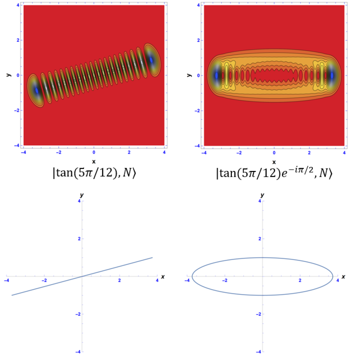
Fig. 22 presents probability densities of the SU(2) coherent state with values of , radians above the equator of the Bloch sphere, and . Comparing these plots with Figs. 15 and 16, it can be seen that the case with , , rotates the figure radians CW from Fig. 15. The case with a phase of , decreases the eccentricity of the figure, but not at the same rate as Fig. 16. is also rotated radians CW such that the semi-major axis is parallel to the -axis. The combination of and rotates the Lissajous figures (both quantum and classical) an additional amount. Just as in the classical Lissajous ellipse, it can be seen that there is one extreme value on both the and axis.
4.2 Fundamental Anisotropic Quantum Lissajous State
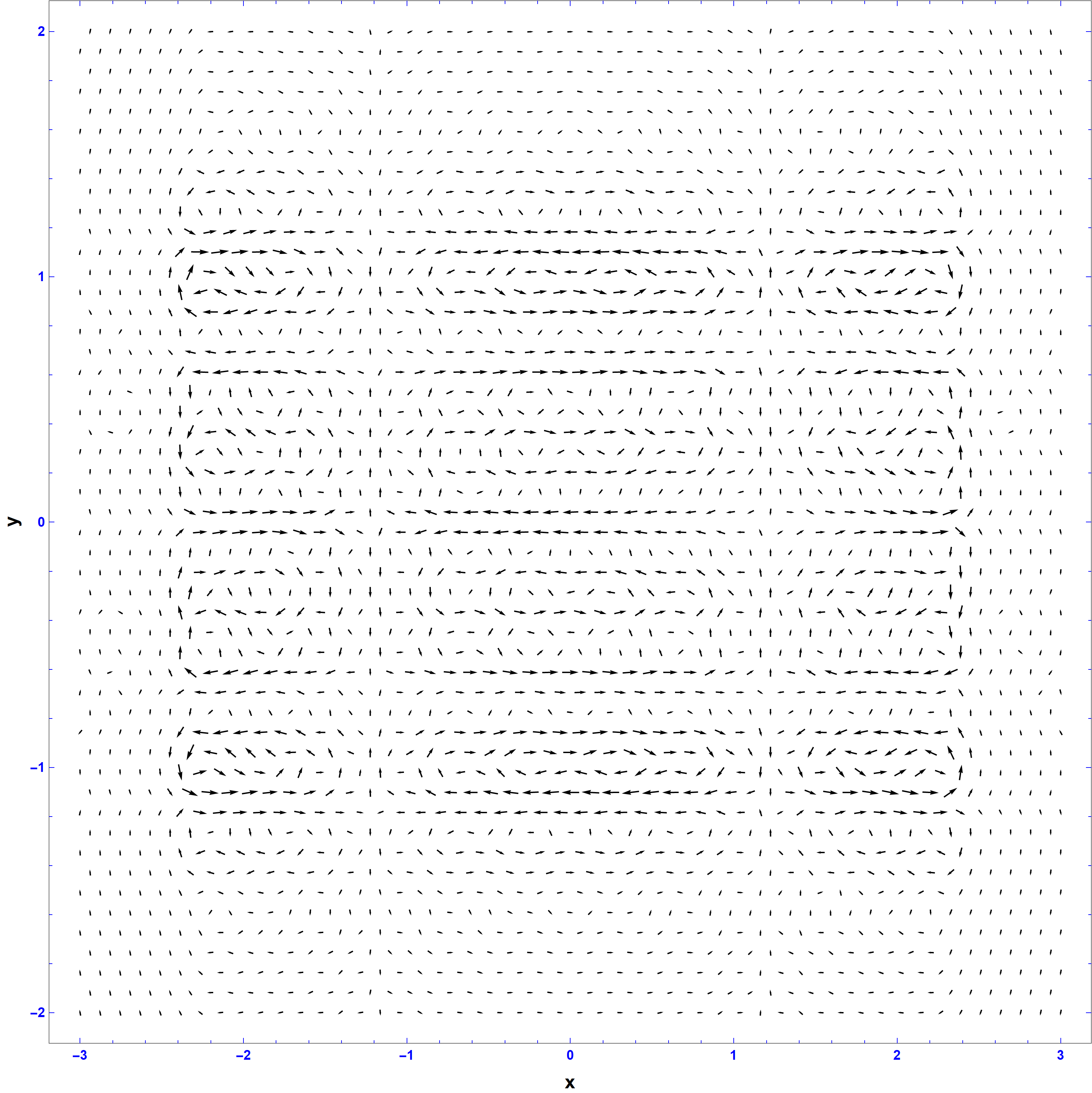
The results presented in this section correspond to the theory developed on the fundamental anisotropic quantum Lissajous states, Eq. (155), and its wavefunction, Eq. (158). The probability density is calculated using Eq. (161) and the probability current density using Eq. (173).
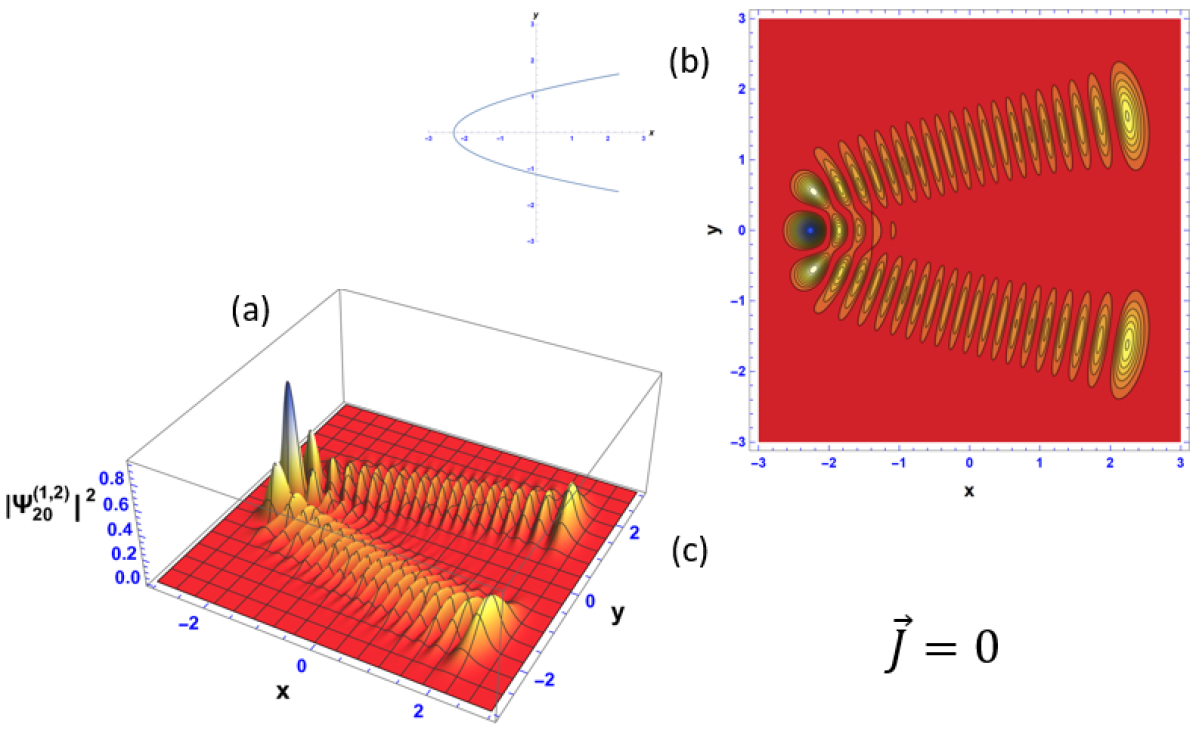
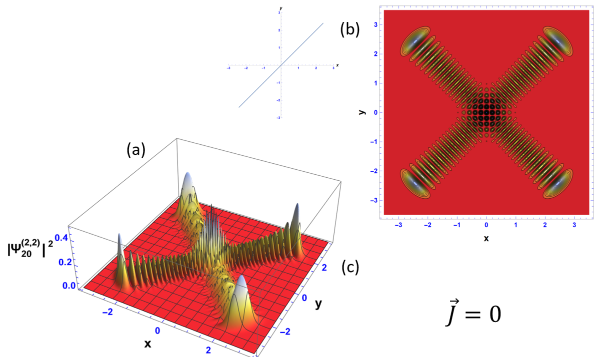
Fig. 23 localizes over the 1:2 classical Lissajous figure for , picture to the left of (b). Similarly to Fig. 15, the probability current density vanishes and the interference fringes are fully resolved. The classical oscillator travels along the path of the 1:2 Lissajous figure and temporally oscillates on that curve, whereas the quantum oscillator’s probability density spatially oscillates along the corresponding classical Lissajous figure. The reasoning for the fully resolved interference fringes is the same as in Fig. 15, thus, this is the static limit of the 1:2 quantum Lissajous states for the anisotropic 2DHO.
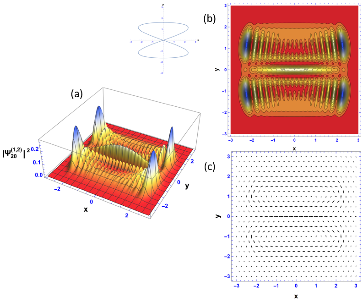
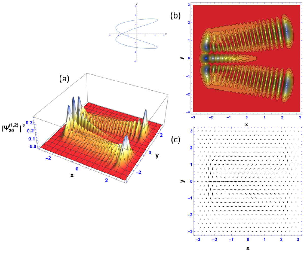
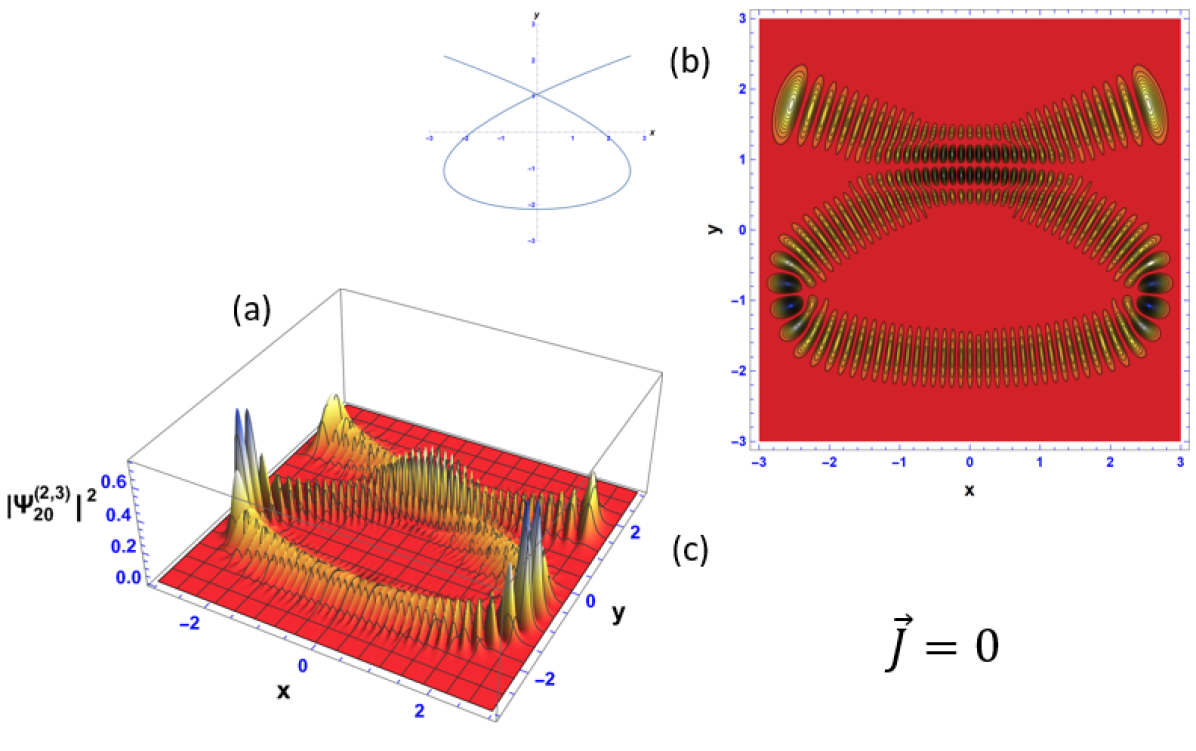
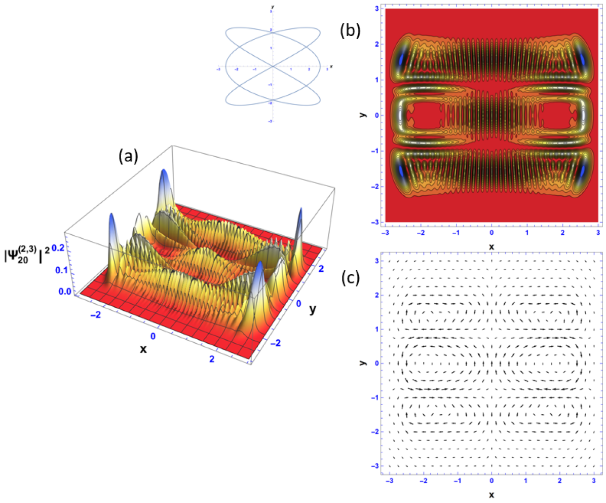
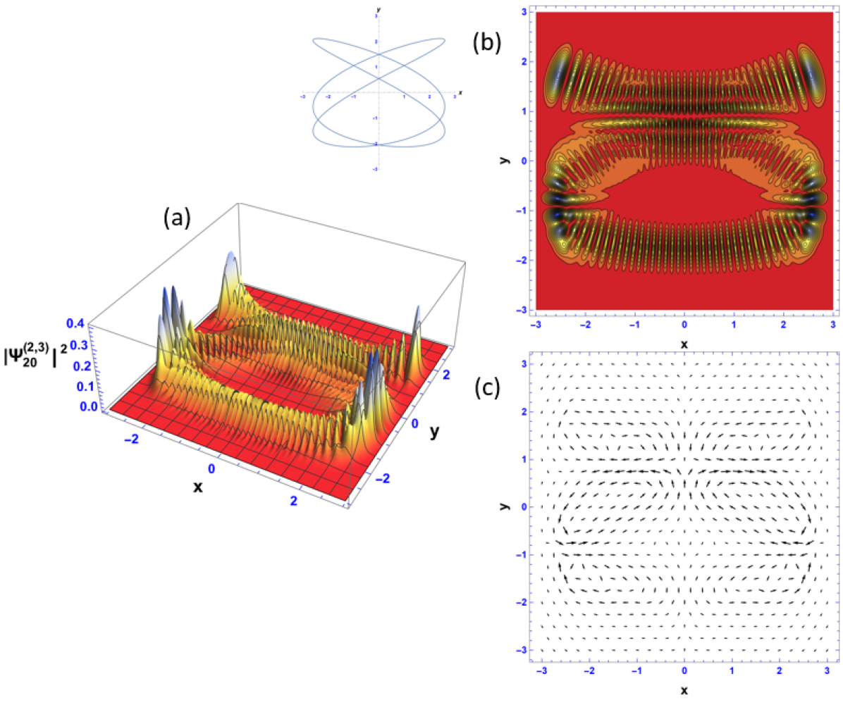
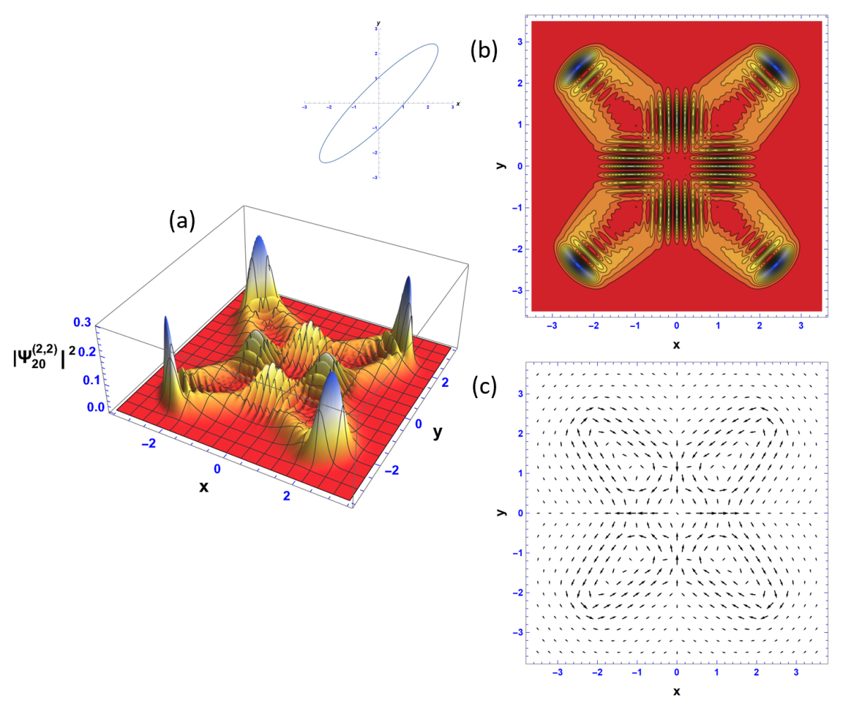
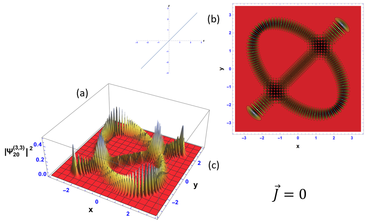
Figs. 23-28 present results of the fundamental anisotropic quantum Lissajous states. The emergence of interference fringes and the connection they have with probability current density comes about in the same way as the fundamental isotropic quantum Lissajous state. A new feature that is observed in the anisotropic probability density and probability current density is the appearance of fringes at the overlaps in the classical Lissajous figure. It can be seen in Figs. 24, 25, 27, and 28 that when there is an overlap in the classical Lissajous figure, this corresponds to a cancellation of probability current in the quantum Lissajous figure in one direction, leaving a horizontal (vertical) stream of current and resulting in vertical (horizontal) interference fringes. Fig. 26 also exhibits interference fringes at the overlap of the classical figure, but the fringes are fully resolved and there are both vertical and horizontal fringes due to the vanishing probability current density. Another new feature is the relationship between and , and the number of vortices present. The number of vortices is proportional to , with columns and rows. There are two vortices in the 1:2 quantum Lissajous state and six vortices in the 2:3 quantum Lissajous state. The number of extrema still holds for quantum Lissajous figures as; extrema on the axis and extrema on the axis, so it can be deduced that extrema on the axis corresponds to columns of vortices and extrema on the axis corresponds to rows of vortices.
4.3 Isotropic Higher Harmonic Quantum Lissajous State
The results presented in this section correspond to the theory developed on the isotropic higher harmonic quantum Lissajous states, Eq. (164), and its wavefunction, Eq. (165). The probability density is calculated using Eq. (167) and the probability current density using Eq. (173).
From Fig. 29, one can observe a coherent superposition of two fundamental isotropic quantum Lissajous states having complex amplitudes that are the square roots of unity. It is clear that this is a coherent superposition and not an incoherent mixture. The overlap of the two separate probability densities has developed interference fringes like the ones seen at that overlap in Fig. 26. Also, based upon Eq. (167), the second term is the interference term. If this were an incoherent mixture, the second term of Eq. (167) would vanish, and the probability density of the 2:2 quantum Lissajous state would simply be the addition of the probability densities of the 1:1 quantum Lissajous figures having amplitudes that are the square roots of unity. As verification of Eq. (167), the incoherent mixture can be plotted,
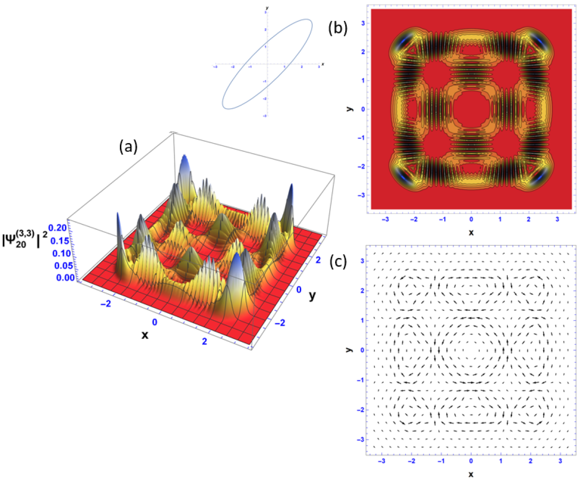
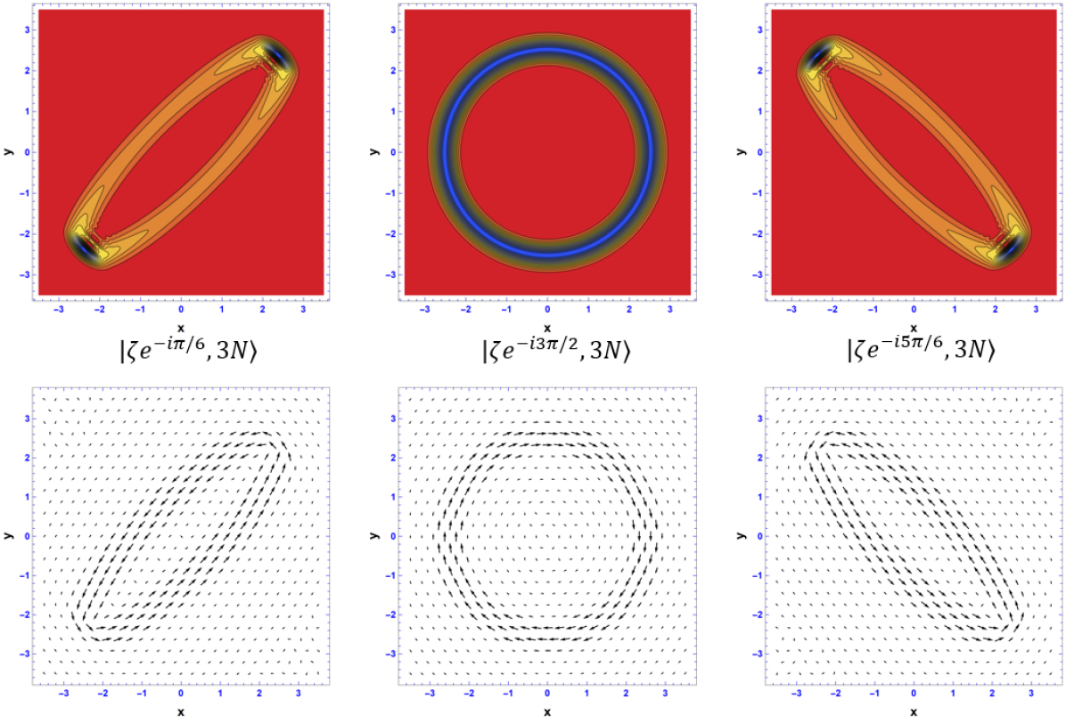
The figures presented in this section are the isotropic higher harmonic quantum Lissajous states. They are formed by a coherent superposition of fundamental isotropic quantum Lissajous states (SU(2) coherent states) with quanta, frequencies of , and complex amplitudes corresponding to the roots of unity, or the roots of unity shifted by an already existing phase, . There is extrema on both the and axis, and vortices when applicable ( columns and rows).
4.4 Anisotropic Higher Harmonic Quantum Lissajous State
The results presented in this section correspond to the theory developed on the isotropic higher harmonic quantum Lissajous states, Eq. (168), and its wavefunction, Eq. (169). The probability density is calculated using the anisotropic higher harmonic analog to Eq. (167) and the probability current density using Eq. (173).
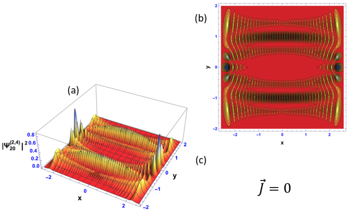
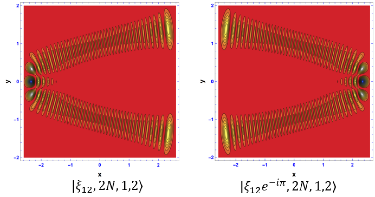
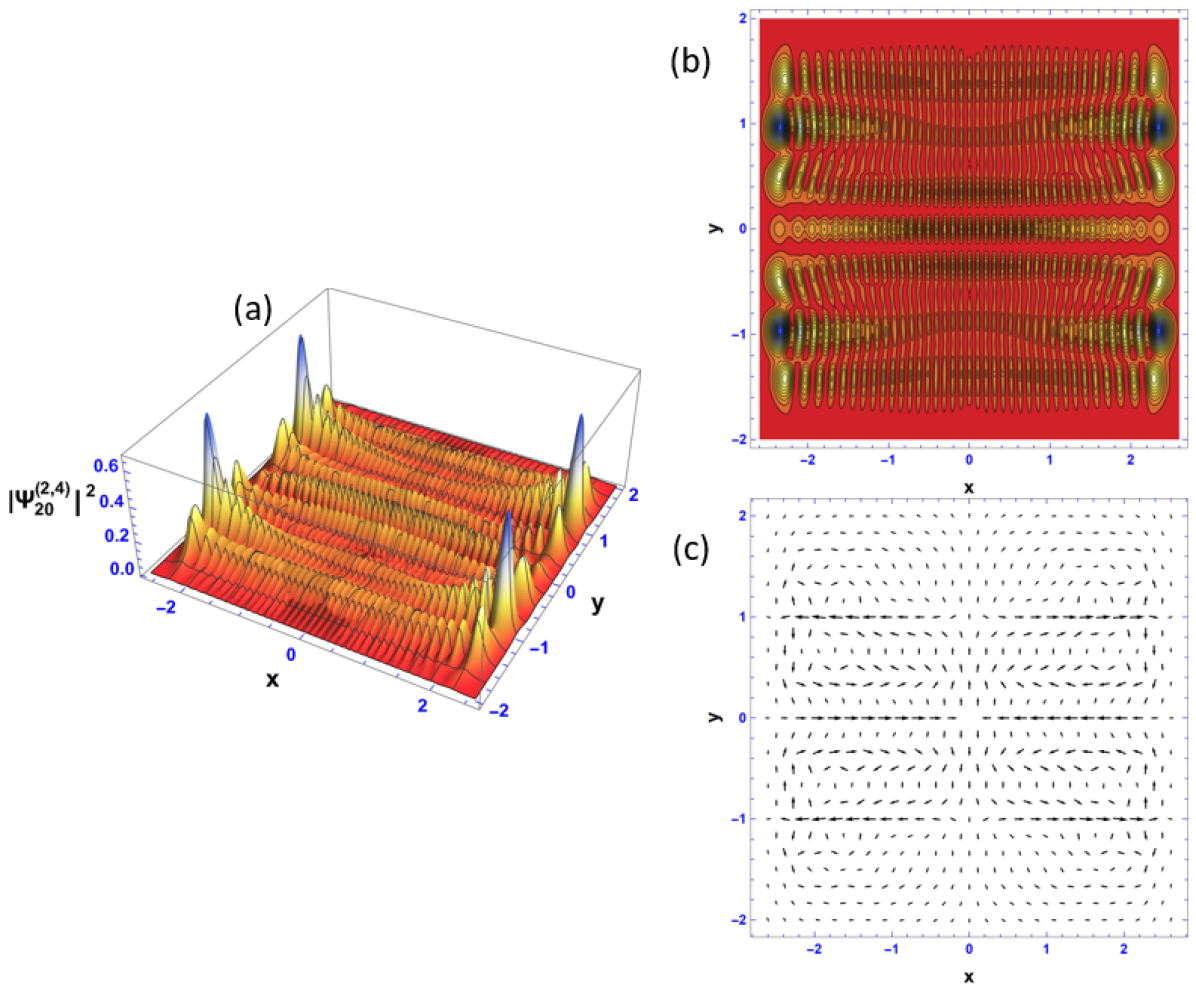
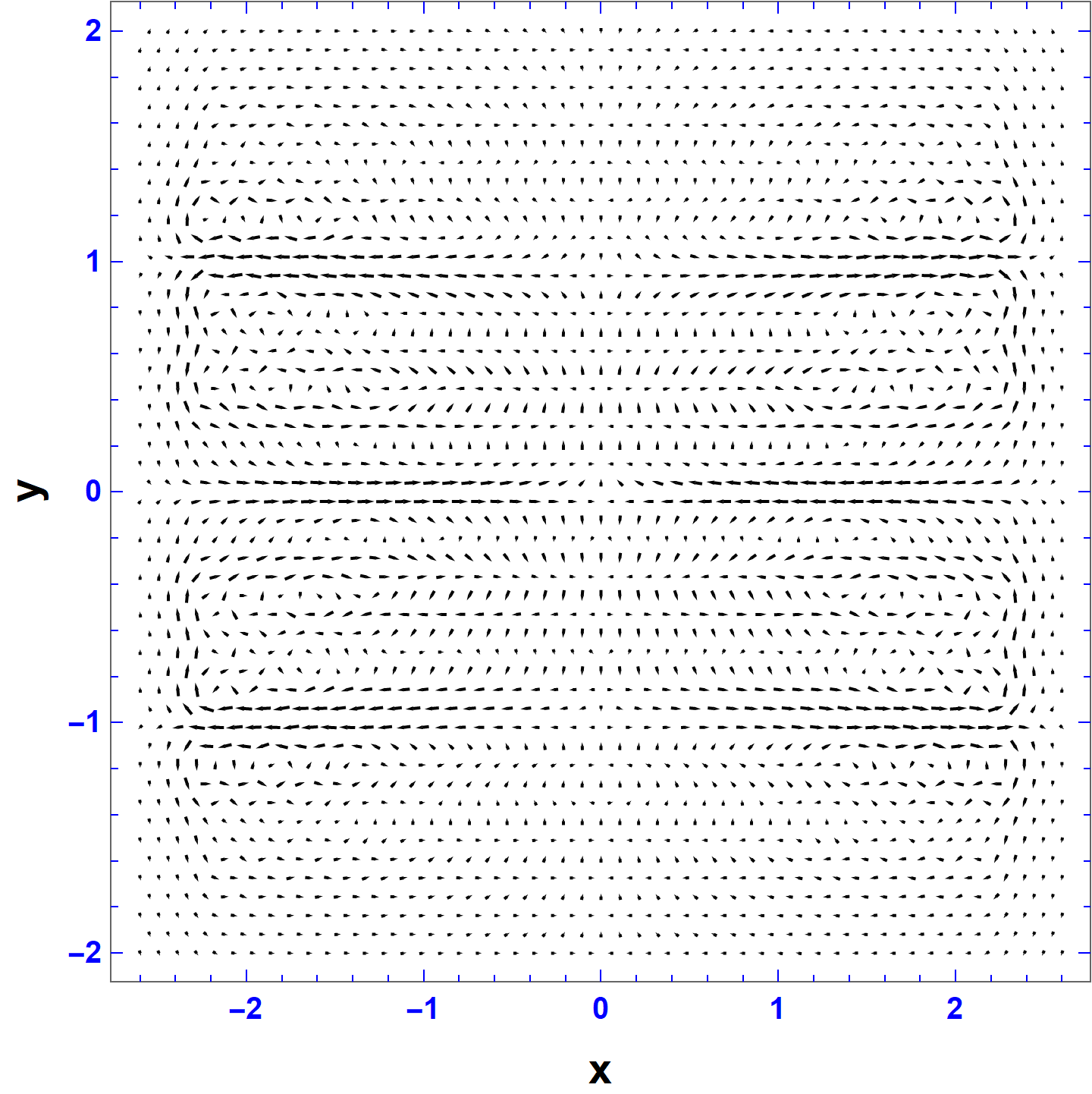
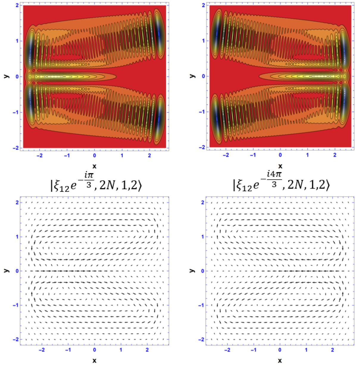
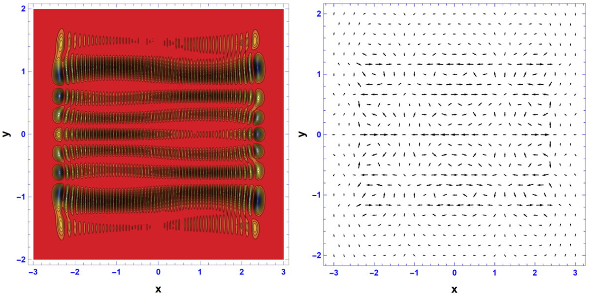
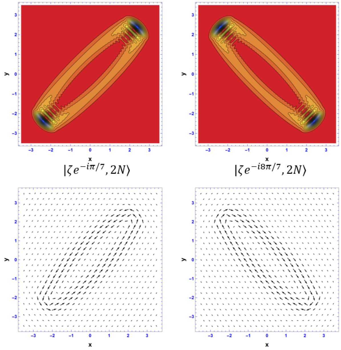
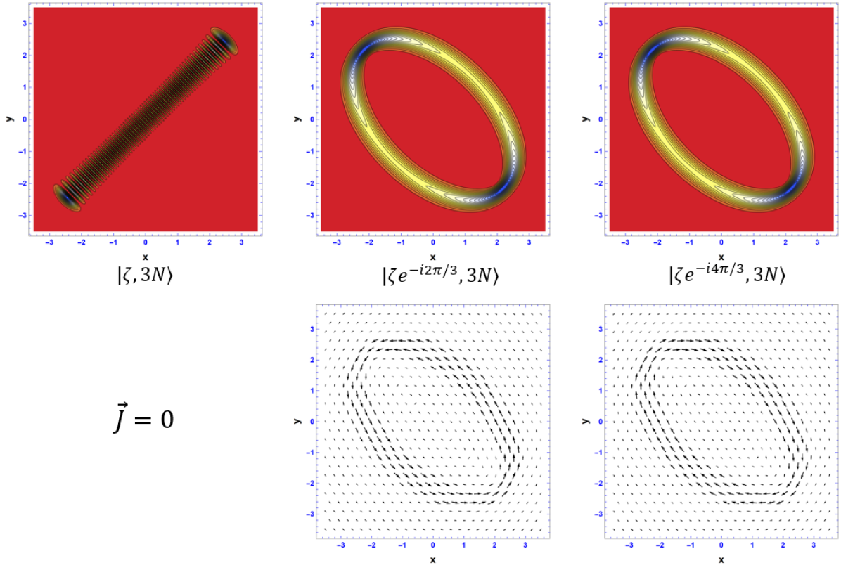
The figures presented in this section are the isotropic higher harmonic quantum Lissajous states. It becomes difficult to visually distinguish which fundamental anisotropic states are in superposition; the 2:4 case being the easiest to discern. They are formed by a coherent superposition of fundamental isotropic quantum Lissajous states (SU(2) coherent states) with quanta, frequencies of , and complex amplitudes corresponding to the roots of unity, or the roots of unity shifted by an already existing phase, . There is extrema on the axis and extrema on the axis, and vortices when applicable ( columns and rows).
5 Summary
We have presented a theoretical framework in which quantum Lissajous figures arise ‘organically’ via projection of a two-mode ordinary coherent state onto a degenerate subspace of the 2DHO. The states resulting from this process are quantum mechanically stationary, having time-independent configuration space probability densities localized along the corresponding classical Lissajous figures. For the isotropic 2DHO, the fundamental case naturally reproduced the SU(2) coherent states; for the anisotropic 2DHO the fundamental cases are not SU(2) coherent states in even a meaningful “generalized” way (as some claim them to be), still the anisotropic fundamental quantum Lissajous states can be used as a non-orthogonal basis for the expansion of anisotropic higher harmonic quantum Lissajous states having the same frequency ratios. This is in direct analogy with the role of the SU(2) coherent states with respect to isotropic higher harmonic cases.
The higher harmonic quantum Lissajous states are radically different from their classical counterparts in one very important way. The classical version is simply a copy of the fundamental case with an times larger frequency, tracing the figure times faster than the relevant fundamental case (same orientation and eccentricity behaviors as the fundamental), owing to the larger amount of mechanical energy in the system. In the quantum version, a linear superposition of the fundamental states relevant of a given case naturally emerges; for the harmonic state the complex amplitudes of the states involved in the superposition are weighted by the roots of unity. We have related the amplitude factors involved to the phases of the originally projected ordinary coherent states. The superposition that arises is the signature of quantum interference in these higher harmonic states, and the evidence for this is clear in our graphical results. We have given a detailed description of the important interplay between quantum mechanical probability current density and quantum interference, especially in connection with the vortex states that arise when considering the quantum Lissajous states. We have pointed out the crucial role played by continuity with respect to the stationary nature of all quantum Lissajous states (both vortex and static). We believe that this discussion sheds light on an issue that seems to have been muddled or ignored in the existing literature on Lissajous figures in quantum mechanics.
Our work has several clear connections and possible extensions: The systematic study of roots-of-unity states for ordinary, SU(2), and SU(1,1) coherent states (we have already done a lot of this but have omitted it from this manuscript). One obvious extension of this work is the examination of quantum Lissajous states via projection in multi-mode systems (e.g., 3DHO, etc.). Another interesting avenue is the investigation of the possibility of quantum stationary states via projection for the “Kepler” problem (H-atom); this is the only other problem that might support them owing to (the Ehrenfest limit of) Bertrand’s theorem. One could also consider the projections of states other than the ordinary coherent states. Do these generally bear any relation to classical Lissajous figures? We don’t know, but this could be the basis for a provable theorem. Systematic study of the non-classical properties and interactions of all types of quantum Lissajous states could yield interesting results for quantum technologies based on integrated nano-photonics and quantum dots. Finally, finding a viable method for producing quantum Lissajous states in the lab would be an essential breakthough for their possible application to possible non-classical systems.
6 Appendix: SU(2) Coherent States
6.1 SU(2) Coherent States in the Angular Momentum Representation
A big theme of this project involves SU(2) coherent states. We have encountered the SU(2) coherent states in a non-traditional way, by projecting the ordinary coherent state onto a degenerate subspace of the 2DHO. This appendix will summarize well known earlier derivations of SU(2) coherent states (Arecchi et al.)[10, 30] in the angular momentum basis. In addition, the Schwinger Realization[13] that, relates the angular momentum operators to the raising and lowering operators of the quantum harmonic oscillator, is implemented to yield the SU(2) coherent state in the Fock state basis.
The angular momentum basis states, just like the Fock states, can be constructed by applying the raising operator on the ground state
| (176) | ||||
where . The angular momentum representation has its own version of raising and lowering operators
| (177) | ||||
and can be written in terms of raising and lowering operators
| (178) | ||||
Eqs. (177) and (178) obey the commutation relations
| (179) | ||||
The Casimir operator for this algebra is , given by Eq. (135). It is important to recall the eigenvalue equations for and
| (180) | ||||
and
| (181) | ||||
Similar to how the ordinary coherent state is created by displacing the ground Fock state, the SU(2) coherent state is created by a rotational "displacement" of the angular momentum ground state. Using the normally ordered form of the rotation operator, the second equality of Eq. (139), one finds
| (182) | ||||
Eq. (182) is the SU(2) coherent state in the angular momentum representation.
6.2 SU(2) Coherent States in the Fock State Representation
Using Eqs. (130) and (133), we can obtain the eigenvalue equations for and in the Fock state basis,
| (183) | ||||
and
| (184) | ||||
Comparing Eqs. (183) and (184) with Eqs. (180) and (181), we can see that
| (185) | ||||
and
| (186) | ||||
A simple substitution of these into Eq. (182) yields the SU(2) coherent state in the Fock state representation, that we found via projection of the two-mode coherent state onto a degenerate subspace of the 2DHO
| (187) | ||||
References
- [1] Jerry B. Marion and Stephen T. Thornton. Classical Dynamics of Particles and Systems. 4th Ed. Fort Worth: Saunders College Pub, 1995. ISBN: 978-0-03-097302-4.
- [2] Herbert Goldstein, Charles P. Poole, and John L. Safko. Classical Mechanics. 3rd Ed. San Francisco Munich: Addison Wesley, 2008. ISBN: 978-0-201-65702-9.
- [3] Max Born and Emil Wolf. Principles of Optics: Electromagnetic Theory of Propagation, Interference and Diffraction of Light. 6th Ed. Oxford; New York: Pergamon Press, 1980. ISBN: 978-0-08-026481-3.
- [4] Jun John Sakurai and Jim Napolitano. Modern Quantum Mechanics. 2nd Ed. Cambridge: Cambridge University Press, 1980. ISBN: 978-1-108-42241-3.
- [5] David H. McIntyre, Corinne A. Manogue and Janet Tate. Quantum Mechanics: A Paradigms Approach. OCLC: ocn727710701. Boston: Pearson, 2012. ISBN: 978-0-321-76579-6.
- [6] P. A. M. Dirac. “Generalized Hamiltonian Dynamics". In: Canadian Journal of Mathematics 2 (1950), pp. 129-148. ISSN: 0008-414X, 1496-4279. DOI: 10.4153/CJM-1950-012-1. URL: https://www.cambridge.org/core/product/identifier/S0008414X00025700/type/journal_article
- [7] Planck Discovers the Quantum of Action URL: https://web.archive.org/web/20080418002757/http://dbhs.wvusd.k12.ca.us/webdocs/Chem-History/Planck-1901/Planck-1901.html
- [8] C. C. Gerry and Peter Knight Introductory Quantum Optics. Cambridge, UK; New York: Cambridge University Press, 2005. ISBN: 978-0-521-52735-4.
- [9] Leonard Mandel and Emil Wolf. Optical Coherence and Quantum Optics. Cambridge; New York: Cambridge University Press, 1995. ISBN: 978-0-521-41711-2.
- [10] F. T. Arecchi et al. “Atomic Coherent States in Quantum Optics". In: Physical Review A 6.6 (Dec. 1972). American Physical Society, pp. 2211-2237. DOI: 10.1103/PhysRevA.6.2211. URL: https://link.aps.org/doi/10.1103/PhysRevA.6.2211.
- [11] Y. N. Demkov. “The Definition of the Symmetry Group of A Quantum System. The Anisotropic Oscillator". In: Soviet Physics JEPT 17 (Jan. 1963), p. 3.
- [12] Y. F. Chen and K. F. Huang. “Vortex Structure of Quantum Eigenstates and Classical Periodic Orbits in Two-Dimensional Harmonic Oscillators". In: Journal of Physics A: Mathematical and General 36.28 (July 2003), pp. 7751-7760. ISSN: 0305-4470, 1361-6447. DOI: 10.1088/0305-4470/36/28/305. URL: https://iopscience.iop.org/article/10.1088/0305-4470/36/28/305.
- [13] Julian Schwinger. On Angular Momentum. Dover Edition. Mineola, New York: Dover Publications, Inc, 2015. ISBN: 978-0-486-78810-4.
- [14] Robert Gilmore. Lie Groups, Lie Algebras, and Some of Their Applications. Mineola, New York: Dover Publications, Inc, 2005. ISBN: 978-0-486-44529-8.
- [15] X. L. He et al. “Fast Generation of Schrodinger Cat States Using a Kerr-Tunable Superconducting Resonator" In: Nature Communications 14.1 (Oct. 2023), p. 6358. ISSN: 2041-1723. DOI: 10.1038/s41467-023-42057-0. URL: https://www.nature.com/articles/s41467-023-42057-0.
- [16] Naeem Akhtar, Barry C. Sanders and Carlos Navarrete-Benlloch. “Sub-Planck Structures: Analogies Between the Heisenberg-Weyl and SU(2) Groups" In: Physical Review A 103.5 (May 2021), arXiv:2102.10791 [quant-ph], p. 053711. ISSN: 2469-9926, 2469-9934. DOI: 10.1103/PhysRevA.103.053711. URL: http://arxiv.org/abs/2102.10791.
- [17] David Jeffrey Griffiths. Introduction to Electrodynamics. 4th Ed. Cambridge: Cambridge University Press, 2017. ISBN: 978-1-108-42041-9.
- [18] V. A. Weilnhammer et al. “Revisiting the Lissajous Figure as a Tool to Study Bistable Perception". In: Vision Research 98 (May 2014), pp. 107-112. ISSN: 00426989. DOI: 10.1016/j.visres.2014.03.013. URL: https://linkinghub.elsevier.com/retrieve/pii/S0042698914000716.
- [19] Aseem Vivek Borkar et al. “Application of Lissajous Curves in Trajectory Planning of Multiple Agents". In: Autonomous Robots 44.2 (Jan. 2020), pp. 233-250. ISSN: 0929-5593, 1573-7527. DOI: 10.1007/s10514-019-09888-7. URL: http://link.springer.com/10.1007/s10514-019-09888-7.
- [20] J. R. Barker, R. Akis and D. K. Ferry. “On the Use of Bohm Trajectories for Interpreting Quantum Flows in Quantum Dot Structures". In: Superlattices and Microstructures 27.5 (May 2000), pp. 319-325. ISSN: 0749-6036. DOI: 10.1006/spmi.2000.0834. URL: https://www.sciencedirect.com/science/article/pii/S0749603600908346.
- [21] J. P. Bird et al. “Intrinsic Stable Orbits in Open Quantum Dots". In: Superconductor Science and Technology 13.8A (Aug. 1998), A4-A6. ISSN: 0268-1242, 1361-6641. DOI: 10.1088/0268-1242/13/8A/003. URL: https://iopscience.iop.org/article/10.1088/0268-1242/13/8A/003.
- [22] K. J. Górska, A. J. Makowski and S. T. Dembiński. “Correspondence Between Some Wave Patterns and Lissajous Figures". In: Journal of Physics A: Mathematical and General 39.42 (Oct. 2006), pp. 13285-13293. ISSN: 0305-4470, 1361-6447. DOI: 10.1088/0305-4470/39/42/006. URL: https://iopscience.iop.org/article/10.1088/0305-4470/39/42/006.
- [23] M. Sanjay Kumar and B. Dutta-Roy. “Commensurate Anisotropic Oscillator, SU(2) Coherent States and the Classical Limit". In: Journal of Physics A: Mathematical and Theoretical 41.7 (Feb. 2008). arXiv:0710.1199 [quant-ph], p. 075306. ISSN: 1751-8113, 1751-8121. DOI: 10.1088/1751-8113/41/7/075306. URL: http://arxiv.org/abs/0710.1199.
- [24] James Moran and Véronique Hussin. “Coherent States for the Isotropic and Anisotropic 2D Harmonic Oscillators". In: Quantum Reports 1.2 (Nov. 2019), pp. 260-270. ISSN: 2624-960X. DOI: 10.3390/quantum1020023. URL: https://www.mdpi.com/2624-960X/1/2/23.
- [25] R. P. Feynman. “Atomic Theory of the Two-Fluid Model of Liquid Helium". In: Physical Review 94.2 (Apr. 1954), pp. 262-277. ISSN: 0031-899X. DOI: 10.1103/PhysRev.94.262. URL: https://link.aps.org/doi/10.1103/PhysRev.94.262.
- [26] L. Onsager. “Statistical Hydrodynamics". In: Il Nuovo Cimento 6.S2 (Mar. 1949), pp. 279-287. ISSN: 0029-6341, 1827-6121. DOI: 10.1007/BF02780991. URL: http://link.springer.com/10.1007/BF02780991.
- [27] Edward A. McCullough and Robert E. Wyatt. “Dynamics of the Collinear H+H2 Reaction. II. Energy Analysis". In: The Journal of Chemical Physics 54.8 (Apr. 1971), pp. 3592-3600. ISSN: 0021-9606, 1089-7690. DOI: 10.1063/1.1675385. URL: https://pubs.aip.org/jcp/article/54/8/3592/214202/Dynamics-of-the-Collinear-H-H2-Reaction-II-Energy.
- [28] Joseph O. Hirschfelder, Albert C. Christoph and William E. Palke. “Quantum Mechanical Streamlines. I. Square Potential Barrier". In: The Journal of Chemical Physics 61.12 (Dec. 1974), pp. 5435-5455. ISSN: 0021-9606, 1089-7690. DOI: 10.1063/1.1681899. URL: https://pubs.aip.org/jcp/article/61/12/5435/779048/Quantum-mechanical-streamlines-I-Square-potential.
- [29] Joseph O. Hirschfelder, Charles J. Goebel and Ludwig W. Bruch. “Quantized Vortices Around Wavefunction Nodes. II". In: The Journal of Chemical Physics 61.12 (Dec. 1974), pp. 5456-5459. ISSN: 0021-9606, 1089-7690. DOI: 10.1063/1.1681900. URL: https://pubs.aip.org/jcp/article/61/12/5456/779046/Quantized-vortices-around-wavefunction-nodes-II.
- [30] Akira Inomata, Hiroshi Kuratsji and Christopher C. Gerry. Path Integrals and Coherent States of SU(2) and SU(1,1). Singapore: World Scientific, 1992. ISBN: 978-981-02-0656-7.