Charge-transport forecasted via deep learning in the photosystem II reaction center

Abstract

Predicting future physical behavior through the limited theoretical simulation data available is an emerging research paradigm resulted by the integration of artificial intelligence technology and quantum physics. In this work, the charge-transport(CT) behavior was forecasted over a long time by a deep learning model, the long short-term memory (LSTM) network with error threshold training method in the photosynthesis II reaction center (PSII-RC). The theoretical simulation data within 8 fs was fed to the modified LSTM network for training, which brings out a distinct prediction with difference of $10^{-4}$ orders of magnitude over a long time period compared to the collection time for training sets. The results indicate the potential of employing LSTM to reveal the physics governing CT in addition to quantum physical methods. The implications of this work warrant further investigation to fully elucidate the scope and efficacy of LSTM for advancing our understanding of photosynthesis at the molecular scale.(Original codes in Supplement information)

PACs

42.50.Gy,42.50.Dv,32.80.Qk

Keywords

Long short-term memory networks, error threshold training method, photosynthesis II reaction center

I Introduction

The traditional theoretical descriptions of quantum open systemsPhysRevLett.103.210401 ; Vacchini2011 are extremely challenging, owing to a huge number of strong coupled degrees of freedom involved. Within the system-plus-bath frameworkshibata1977reduced ; rivas2012open , the quantum evolution of the target reduced system takes precedence over that of the environmental degrees of freedom. Consequently, it is crucial to develop a suitable dynamics approach that can accurately describe the quantum evolution of open systems. Thus, many dynamical approaches were proposed to the quantum open systems. For example, the perturbative approachesfleming2012perturbation ; strathearn2018high , such as Redfield theorypurkayastha2021beyond ; stace2021redfield ; trushechkin2021redfield , work well in cases of weak system-bath coupling. To obtain an accurate description of the quantum evolution of open systems, several numerically exact dynamics approaches have been developed. These include the hierarchical equations of motion (HEOM) methodtanimura2020efficient ; wiedmann2020modular ; tang2021hierarchical ; erpenbeck2021hierarchical , the hybrid stochastic-deterministic HEOMtang2020hybrid , the multi-configurational time-dependent Hartree (MCTDH) techniquewang2020multi ; farag2021multi and its multi-layer extension (MLMCTDH)schroder2022multi , as well as tensor-network decomposition methodschin2020tensor .

These advanced approaches allow for the precise modeling of open quantum systems, going beyond the limitations of perturbative methods like Redfield theory, which struggles in the strong system-bath coupling regime. Although they are widely regarded as rigorous approaches to simulate open quantum dynamics, these methods are often constrained by convergence problem or high computational costschuch2019convergence ; chen2021overcoming . Therefore, it remains highly desirable to develop a new theoretical framework that can provide a reliable description of open quantum dynamics with high computational efficiency, without being restricted to specific model parameter regions. In recent years, as powerful techniques that can extract the essential features of input raw data and make the prediction of unknown outputs, machine learning algorithms (ML) have been widely used in various scientific and technological domainsschmidt2019machine ; elton2019deep ; dunjko2018machine ; ntampaka2019machine . Meanwhile, artificial neural networks have been used in quantum physics, especially in quantum dissipative processes of complex systemspalmieri2020quantum . A well-trained ML model can make a rapid forecasting while ensuring a high prediction accuracy, where its prediction cost and accuracy are determined by the training data and the training processrodrigues2020artificial ; carleo2017solving . Therefore, it is challenging for ML applications in physics to generate highly accurate and powerful ML models while not sufficient data set.

In contrast to standard feed-forward neural networks, long short-term memory (LSTM) architectureszhu2022long have recurrent connections, which can avoid the unexpected vanishing and exploding gradient problems and model the long-range dependencies of the time-series data set, make the forecasting for the future unseen datalim2021review . Such sequence-processing capabilities can better capture the features of sequence data, improving the model’s prediction accuracy and effectiveness. Thus, LSTM neural networks (LSTM-NNs) have been widely used in various types of time-series analysis and forecasting problemstaieb2018forecasting ; lai2018modeling , such as the long-time dissipative dynamics of open quantum systemsgarciaperez2021machine ; potocnik2022forecasting .

In this work, the LSTM-NN was employed to forecast the long-term CT behavior in PSII-RC with a smaller training data from the quantum master equation, in contrast to the extensive theoretical analyses. In order to meet the specific needs of CT prediction, the LSTM model structure hyperparameters were designed and optimized, such as the network layers, forget gates, input gates, and output gates. And a long-term CT forecasting will be achieved by our proposed LSTM model with a high precision.

II Dataset collection from Photosystem II reaction center (PSII-RC)

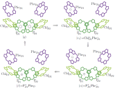
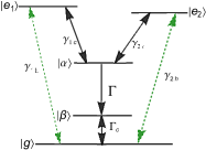
Figure 1: (a) Four typical sates in the charge-transfer processauthor2021charge . On the channel of $|g\rangle$$\rightarrow$$|e_{1}\rangle$$\rightarrow$$|\alpha\rangle$$\rightarrow$$|\beta\rangle$$\rightarrow$$|g\rangle$) of the six core-pigments in the PSII RC. $|g\rangle$, six pigments in neutral ground state. $|e_{1}\rangle$=Chl${}^{+}_{D1}$Phe${}_{D1}^{-}$ after Chl_D1 primary charge-transfer state when the electron donor rapidly loses an electron to the nearby electron acceptor molecule Phe_D1. $|\alpha\rangle$=P${}_{D1}^{+}$Phe${}_{D1}^{-}$ charge-transfer state, after the positive and negative charges are spatially separated. $|\beta\rangle$=P${}_{D1}^{+}$Phe_D1, positively charged state, after an electron has been released from the system to perform work. (b) Corresponding five-level diagram of the photosynthetic QHE model with two photon-absorbing channels $|g\rangle$ to $|e_{1}\rangle$ and $|e_{2}\rangle$. $\gamma_{1h}$ and $\gamma_{2h}$ are the transition rates corresponding, $|\alpha\rangle$ is the charge separation state characterized by the transition rate $\gamma_{1h}(\gamma_{2h})$ from state $|e_{1}\rangle(|e_{2}\rangle)$ to state $|\alpha\rangle$, and the relaxation rate $\Gamma$ to state $|\beta\rangle$, $\Gamma_{C}$ is the relaxation rate to the ground state $|g\rangle$ of the system.

The typical PSII-RC found in purple bacteria and oxygen-evolving organisms contains six pigment molecules aligned in two branches2015Multiple ; author2021charge , which contains four chlorophylls (special pair P_D1 and P_D2 and accessory Chl_D1 and Chl_D2) and two pheophytins (Phe_D1 and Phe_D2) arranged in two branchesM2017Effects . As shown in Fig.1 (a), $|g\rangle$ denotes all six pigments in neutral ground state after an electron has been replenished at the special pair. $|e_{1}\rangle$=Chl${}^{+}_{D1}$Phe${}_{D1}^{-}$ describes primary charge-transfer state after Chl_D1 when the electron donor rapidly loses an electron to the nearby electron acceptor molecule Phe_D1. $|\alpha\rangle$ represents charge-transfer state P${}_{D1}^{+}$Phe${}_{D1}^{-}$ with the positive and negative charges spatially separated. And $|\beta\rangle$ expresses positively charged state, P${}_{D1}^{+}$Phe_D1 after an electron has been released out of the system to perform work. Fig.1 (b) shows a five-level photosynthetic QHE model corresponding to Fig.1 (a). The charge transfer initiates the photon-absorbing from $|g\rangle$ to $|e_{1}\rangle$ and $|e_{2}\rangle$ with transition rates $\gamma_{1h}$ and $\gamma_{2h}$, respectively. And the charge-separated processes $|e_{1}\rangle$$\leftrightarrow$$|\alpha\rangle$$\leftrightarrow$$|\beta\rangle$, $|e_{2}\rangle$$\leftrightarrow$$|\alpha\rangle$$\leftrightarrow$$|\beta\rangle$ take place at the rate $\gamma_{1c}$ and $\gamma_{2c}$, respectively. With these knowledge, the integral Hamiltonian for the PSII RC plus the ambient environment can be represented by

$$\hat{H}=\hat{H}_{S}+\hat{H}_{B}+\hat{H}_{SB},$$ (1)

where the electronic Hamiltonian with the energy $E_{i}$ of the ith state is read as

$$\hat{H}_{S}= E_{0}|g\rangle\langle g|+E_{e_{1}}|e_{1}\rangle\langle e_{1}|+E_{e_{2}}|e_{2}\rangle\langle e_{2}|$$ (2)

$$+E_{\alpha}|\alpha\rangle\langle\alpha|+E_{\beta}|\beta\rangle\langle\beta|,$$

Among Eq.(2), $\hat{H}_{B}$ describes the Hamiltonian of the ambient thermal bath. Considering the weak coupling between the PSII RC and the ambient environment, the harmonic oscillator thermal bath model is generally introduced to describe the ambient environment as follows,

$$\hat{H}_{B}=\sum_{k}\hbar\omega_{k}\hat{a}^{{\dagger}}_{k}\hat{a}_{k},$$ (3)

where $\hat{a}^{{\dagger}}_{k}(\hat{a}_{k})$ are the creation (annihilation) operator of the k-th harmonic oscillator mode with its frequency $\omega_{k}$. In Eq.(2), $\hat{H}_{SB}$ describes the interaction Hamiltonian between the corresponding ambient reservoir modes and the PSII RC. Under the rotating-wave approximations, $\hat{H}_{SB}$ is expressed as follows,

$$\hat{H}_{SB}=\hat{V}_{h}+\hat{V}_{c},$$

$$\hat{V}_{h}=\sum_{i=1,2}\sum_{k}\hbar(\varepsilon_{ik}\hat{\sigma}_{gi}\otimes\hat{a}_{k}^{{\dagger}}+\varepsilon_{ik}^{\ast}\hat{\sigma}_{gi}^{{\dagger}}\otimes\hat{a}_{k}),$$

$$\hat{V}_{c}=\sum_{j=1,2}\sum_{k}\hbar(\varepsilon_{jk}\hat{\sigma}_{\alpha j}\otimes\hat{b}_{k}^{{\dagger}}+\varepsilon_{jk}^{\ast}\hat{\sigma}_{\alpha j}^{{\dagger}}\otimes\hat{b}_{k}).$$ (4)

where $\varepsilon_{ik}(\varepsilon_{jk})$ is the corresponding coupling-strength between the i(j)th_(i,j=1,2) charge transfer process and the kth mode of ambient environment reservoir, and the transit operators are defined as $\hat{\sigma}_{gi}=|g\rangle\langle e_{i}|$, $\hat{\sigma}_{\alpha j}$=$|\alpha\rangle\langle e_{j}|_{(i,j=1,2)}$ with $\hat{a}^{{\dagger}}_{k}$, $\hat{b}^{{\dagger}}_{k}(\hat{a}_{k}$, $\hat{b}_{k})$ being the creation(annihilation) operators of the k-th reservoir mode, respectively. Under the Born-Markov and Weisskopf-Wigner approximations in the Schr$\ddot{o}$dinger picture, the PSII RC can be described by the master equation deduced by the conventional second-order perturbative treatment for $\hat{V}_{h}$ and $\hat{V}_{c}$. Taking the Lindblad-type superoperators, the master equation is read as,

$$\frac{d\hat{\rho}}{dt}=-i[\hat{H}_{S},\hat{\rho}]+\sum_{i,j=1,2}\mathscr{L}_{ijh}\hat{\rho}+\mathscr{L}_{ijc}\hat{\rho}+\mathscr{L}_{\Gamma_{C}}\hat{\rho}+\mathscr{L}_{\Gamma}\hat{\rho},$$ (5)

In Eq.(5), the first term on the right side describes the coherent evolution of the PSII RC, and the other four Lindblad-type superoperator terms are deduced with the following expressions,

$$\mathscr{L}_{ijh}\hat{\rho}= \sum_{i,j=1,2}\frac{\gamma_{ijh}}{2}[(n_{ih}+1)(\hat{\sigma}_{gi}\hat{\rho}\hat{\sigma}_{gj}^{{\dagger}}+\hat{\sigma}_{gj}\hat{\rho}\hat{\sigma}_{gi}^{{\dagger}}-\hat{\sigma}_{gj}^{{\dagger}}\hat{\sigma}_{gi}\hat{\rho}-\hat{\rho}\hat{\sigma}_{gj}^{{\dagger}}\hat{\sigma}_{gi})$$ (8)

$$+n_{ih}(\hat{\sigma}_{gi}^{{\dagger}}\hat{\rho}\hat{\sigma}_{gj}+\hat{\sigma}_{gj}^{{\dagger}}\hat{\rho}\hat{\sigma}_{gi}-\hat{\sigma}_{gj}\hat{\sigma}_{gi}^{{\dagger}}\hat{\rho}-\hat{\rho}\hat{\sigma}_{gj}\hat{\sigma}_{gi}^{{\dagger}})],$$

$$\mathscr{L}_{ijc}\hat{\rho}= \sum_{i,j=1,2}\frac{\gamma_{ijc}}{2}[(n_{ic}+1)(\hat{\sigma}_{\alpha i}\hat{\rho}\hat{\sigma}_{\alpha j}^{{\dagger}}+\hat{\sigma}_{\alpha j}\hat{\rho}\hat{\sigma}_{\alpha i}^{{\dagger}}-\hat{\sigma}_{\alpha j}^{{\dagger}}\hat{\sigma}_{\alpha i}\hat{\rho}-\hat{\rho}\hat{\sigma}_{\alpha j}^{{\dagger}}\hat{\sigma}_{\alpha i})$$

$$+n_{ic}(\hat{\sigma}_{\alpha i}^{{\dagger}}\hat{\rho}\hat{\sigma}_{\alpha j}+\hat{\sigma}_{\alpha j}^{{\dagger}}\hat{\rho}\hat{\sigma}_{\alpha i}-\hat{\sigma}_{\alpha j}\hat{\sigma}_{\alpha i}^{{\dagger}}\hat{\rho}-\hat{\rho}\hat{\sigma}_{\alpha j}\hat{\sigma}_{\alpha i}^{{\dagger}})],$$

$$\mathscr{L}_{\Gamma_{C}}\hat{\rho}= \frac{\Gamma_{C}}{2}[(N_{C}+1)(2\hat{\sigma}_{g\beta}\hat{\rho}\hat{\sigma}_{g\beta}^{{\dagger}}-\hat{\sigma}_{g\beta}^{{\dagger}}\hat{\sigma}_{g\beta}\hat{\rho}-\hat{\rho}\hat{\sigma}_{g\beta}^{{\dagger}}\hat{\sigma}_{g\beta})$$

$$+N_{C}(2\hat{\sigma}_{\beta g}^{{\dagger}}\hat{\rho}\hat{\sigma}_{\beta g}-\hat{\sigma}_{\beta g}\hat{\sigma}_{\beta g}^{{\dagger}}\hat{\rho}-\hat{\rho}\hat{\sigma}_{\beta g}\hat{\sigma}_{\beta g}^{{\dagger}})],$$

$$\mathscr{L}_{\Gamma}\hat{\rho}= \frac{\Gamma}{2}(2\hat{\sigma}_{\beta\alpha}\hat{\rho}\hat{\sigma}_{\beta\alpha}^{{\dagger}}-\hat{\sigma}_{\beta\alpha}^{{\dagger}}\hat{\sigma}_{\beta\alpha}\hat{\rho}-\hat{\rho}\hat{\sigma}_{\beta\alpha}^{{\dagger}}\hat{\sigma}_{\beta\alpha})$$ (9)

$\mathscr{L}_{ijh}\hat{\rho}$ in the expression (8) denotes the dissipative effect of the ambient environment photon reservoirs. And $\gamma_{iih}$=$\gamma_{ih}$, $\gamma_{jjh}$=$\gamma_{jh}$ are the spontaneous decay rates from the state $|e_{i}\rangle(i$=$1,2)$ to the neutral ground state $|g\rangle$ respectively. $\gamma_{ijh}$=$\gamma_{jih}$, the cross-coupling describes the effect of Fano interference. It is assumed that $\gamma_{ijh}$=$\sqrt{\gamma_{ih}\gamma_{jh}}(i,j$=$1,2)$ represents the maximal interference and $\gamma_{ijh}$=$0$ for the minimal interference. And $n_{ih}(i$=$1,2)$ denotes the average electron occupations on the corresponding charge separation state. The expression $\mathscr{L}_{ijc}\hat{\rho}$ describes the effect of the low temperature reservoirs with the average phonon numbers $n_{ic}$=$[exp(\frac{(E_{e_{i}}-E_{\alpha})}{k_{B}T_{a}})-1]^{-1}(i$=$1,2)$ and $T_{a}$ being the ambient temperature. $\gamma_{iic}$=$\gamma_{ic}$, $\gamma_{jjc}$=$\gamma_{jc}$ are the corresponding spontaneous decay rates from the state $|e_{i}\rangle(i$=$1,2)$ to state $|\alpha\rangle$. $\gamma_{ijc}$ is the cross-coupling that represents the effect of Fano interference, which is defined by $\gamma_{ijc}$=$\gamma_{jic}$$=$$\gamma_{ijc}$=$\sqrt{\gamma_{ic}\gamma_{jc}}(i,j$=$1,2)$ with fully interference while $\gamma_{ijc}=0$ for no interference. Similarly, $\mathscr{L}_{\Gamma_{C}}\hat{\rho}$ in expression (8) describes another interaction between the PSII RC and ambient environment with $\hat{\sigma}_{g\beta}=|\beta\rangle\langle g|$, where $N_{C}$=$[exp(\frac{(E_{\beta}-E_{g})}{k_{B}T_{a}})-1]^{-1}$ denotes the corresponding average phonon occupation numbers. The last term $\mathscr{L}_{\Gamma}\hat{\rho}$ describes a process that the PSII RC in state $|\alpha\rangle$ decays to state $|\beta\rangle$. It leads to the photosynthetic power current proportional to the relaxation rate $\Gamma$ as defined before, and the operator $\hat{\sigma}_{\beta\alpha}$ is defined as $\hat{\sigma}_{\beta\alpha}$=$|\beta\rangle\langle\alpha|$. Thereupon, the elements of the density matrix $\rho$ can be written as follows,

$$\dot{\rho}_{e_{1}e_{1}}={} -\gamma_{1h}[(n_{1h}+1)\rho_{e_{1}e_{1}}-n_{1h}\rho_{gg}]-\gamma_{1c}[(n_{c}+1)\rho_{e_{1}e_{1}}-n_{c}\rho_{\alpha\alpha}]$$

$$-\gamma_{12h}[(n_{1h}+1)Re[\rho_{e_{1}e_{2}}]-\gamma_{12c}[(n_{c}+1)Re[\rho_{e_{1}e_{2}}],$$

$$\dot{\rho}_{e_{2}e_{2}}={} -\gamma_{2h}[(n_{2h}+1)\rho_{e_{2}e_{2}}-n_{1h}\rho_{gg}]-\gamma_{2c}[(n_{c}+1)\rho_{e_{2}e_{2}}-n_{c}\rho_{\alpha\alpha}]$$

$$-\gamma_{12h}[(n_{2h}+1)Re[\rho_{e_{1}e_{2}}]-\gamma_{12c}[(n_{c}+1)Re[\rho_{e_{1}e_{2}}],$$

$$\dot{\rho}_{\alpha\alpha}={} -\gamma_{1c}[(n_{c}+1)\rho_{e_{1}e_{1}}-n_{c}\rho_{\alpha\alpha}]+\gamma_{2c}[(n_{c}+1)\rho_{e_{2}e_{2}}-n_{c}\rho_{\alpha\alpha}]$$

$$+2\gamma_{12c}[(n_{c}+1)Re[\rho_{e_{1}e_{2}}]-\Gamma\rho_{\alpha\alpha},$$ (10)

$$\dot{\rho}_{\beta\beta}={} \Gamma\rho_{\alpha\alpha}-\Gamma_{C}[(\emph{N}_{C}+1)\rho_{\beta\beta}+\emph{N}_{C}\rho_{gg}],$$

$$\dot{\rho}_{e_{1}e_{2}}={} -\frac{\gamma_{1h}}{2}(n_{1h}+1)\rho_{e_{1}e_{2}}-\frac{\gamma_{2h}}{2}(n_{2h}+1)\rho_{e_{1}e_{2}}-\frac{\gamma_{12h}}{2}[(n_{1h}+1)\rho_{e_{1}e_{1}}+(n_{2h}+1)\rho_{e_{2}e_{2}}$$

$$-n_{1h}\rho_{gg}-n_{2h}\rho_{gg}]-\frac{\gamma_{1c}+\gamma_{2c}}{2}(n_{c}+1)\rho_{e_{1}e_{2}}$$

$$-\frac{\gamma_{12c}}{2}[(n_{c}+1)\rho_{e_{1}e_{1}}+(n_{c}+1)\rho_{e_{2}e_{2}}-2n_{c}\rho_{\alpha\alpha}].$$

where $\rho_{ii}$ describe the diagonal element and $\rho_{ij}$ is the non-diagonal element of the corresponding states.

Table 1: Model parameters used in the numerical calculations.

	Values	Units
$E_{1}-E_{\alpha}$	0.2	eV
$E_{\beta}-E_{g}$	0.2	eV
$\gamma_{1h}$	0.62	eV
$\gamma_{2h}$	0.56	eV
$\gamma_{1c}$	0.22	eV
$\gamma_{2c}$	0.82	eV
$\Gamma$	0.56	eV
$\Gamma_{C}$	0.68	eV
$n_{1h}$	60
$n_{2h}$	58
$T_{a}$	300	K

II.1 Structure for LSTM

Compared to traditional recurrent neural networks (RNNs) shi2020analysis , which have the capability of passing information from the past through hidden states across time series, RNNs suffer from the problem of exponential decay or growth of gradients due to the backpropagation process over time. LSTM networkshalpern2020training , on the other hand, effectively address the gradient vanishing problem by incorporating a series of gated mechanisms. The gated mechanisms in LSTM networks enhance the capability to capture long-term dependencies in sequence data.

Within the framework of LSTMswang2021software , the core architecture is composed of a series of interconnected recurrent units, each containing specialized gate control units and a continuous memory cellsmagulova2018memristor . Each LSTM unit includes the following core components internally:

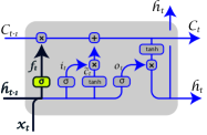
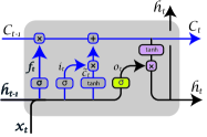
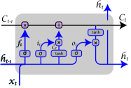
Figure 2: The internal structures and operating mechanisms of (a) forget gate, (b) input gate, (c) output gate, (d) memory cell in LSTM networks.

$$f_{t}=\sigma(W_{f}\cdot[h_{t-1},x_{t}]+b_{f}),$$ (11)

$$i_{t}=\sigma(W_{i}\cdot[h_{t-1},x_{t}]+b_{i}),$$ (12)

$$\tilde{C}_{t}=\tanh(W_{C}\cdot[h_{t-1},x_{t}]+b_{C}),$$ (13)

$$o_{t}=\sigma(W_{o}\cdot[h_{t-1},x_{t}]+b_{o}),$$ (14)

$$C_{t}=f_{t}\circ C_{t-1}+i_{t}\circ\tilde{C_{t}},$$ (15)

$$h_{t}=o_{t}\circ\tanh(C_{t}).$$ (16)

where $\sigma$ is the sigmoid function, the product of the transverse weight matrix$[W_{h},W_{x}]$ (generated by $\mathbf{W}$) and the column matrix $[h_{t-1},x_{t}]$ is used to control the opening of each gate, and $b$ is the bias term. In LSTMs, the weight matrices and bias terms for each gate unit are adjusted to determine the networks response to various inputs during the iterative training processeskala2022forecasting . During training, the network makes predictions through forward propagation, measures performance by calculating the loss between predicted and actual values, and then uses the backpropagation algorithm to compute gradients for adjusting each weight.

As shown in Fig.2(a) and Eq.(11), the forget gate takes the output of the previous hidden state $h_{t-1}$ and the current input $x_{t}$, and passes them through a sigmoid function which determines how much information will be output via its values between 0 and 1 in the cell state $C_{t-1}$. If the sigmoid function outputs 1 for a certain cell state, it indicates that all information is retained. Conversely, if the sigmoid function outputs a value of 0, it signifies that all information is discarded. The input gate shown in Fig.2(b) and Eq.(13) is responsible for updating the cell state via a combination of two operations: a sigmoid function that selects which values to pass through, and a tanh function that creates a vector of new added candidate values, $\tilde{C_{t}}$. Then, the cell state $C_{t}$ is updated by an element-wise multiplication of these two vectors.

In the LSTM network, the output gate determines the next hidden state $h_{t}$ via the current cell state. As shown in Fig.2(c) and Eq.(14), the tanh of the cell state is multiplied by the sigmoid function of the gate’s activation, determining the information that is carried forward by the hidden state. Thus, the value of the next hidden state is filtered by the gate. The memory unit $C_{t}$ is responsible for carrying information in multiple processing steps and has the ability to add or remove information, which is regulated by various gating structuresarunkumar2021forecasting shown by Fig.2(d) and Eq.(15) in an LSTM module. Through this structure, the memory unit can maintain or forget information in long-term sequences, affecting the processing of long-term dependencies.

CT was usually described by the population evolution in PSII-RC. In this work, a predictive system that can capture the dynamic behaviors of population evolution in PSII-RC with high accuracy and stability in long term will be desired, and the above attributes of LSTM offer an approach for predicting the long-term evolution of EET. During the construction of the LSTM model, the Adam optimizerchang2019electricity ; huang2023ultra was employed for enhancing the training efficiency and predictive performance, due to its adaptive learning rate feature and estimates of the first and second moments. What’s more, the early stop functionzhou2022carbon and L2 regularization technologywang2022front ; gao2023l2 with regularization coefficient setting as 0.01 was employed to the LSTM model, preventing overfitting and reducing model complexity.

III RESULTS AND DISCUSSIONS

III.1 Training the LSTM with error threshold training method

In this work, a key step is to collect a verifiable set of actual data for the accuracy, reliability and stability of the deep learning model. Then, an actual data set with ten thousand data points within 10 fs was collected by the Lindblad master equation (5) through Eqs.(10), which describes the CT behavior via the dynamical evolution of populations in PSII-RC with the model parameters outlined in Table (1). And the data were divided into the training and test sets in an 80:20 ratio, i.e., where the first 8000 data points were used to training deep learning model, and the remaining 2000 points were used for testing.

To evaluate the proposed model against specific standards, an innovative training approach was adopted in this work. We use the trained model to predict 10 points and compare these predictions to the corresponding actual values derived from the test set. We set a 0.0005 error threshold. If all 10 test predictions are below this threshold, the model is saved as it has achieved our desired accuracy. If any predictions exceed the threshold, the model is retrained again. For individual predictions, we simply invoke the saved model. This threshold-based early stopping technique reduces training time and computational costs. Importantly, it provides a clear stopping criterion, avoiding guesswork and unnecessary iterations-especially beneficial for complex data sets. This ensures the model’s generalizability and practical prediction stability and reliability. It can also identify and prevent overfitting early, as the model aims for high-precision predictions on specific test points, not just overall loss minimization. In contrast to traditional training that optimizes loss on the entire data set, our method focuses on prediction accuracy for a small test batch, and this concentrated evaluation better reflects real-world performance.

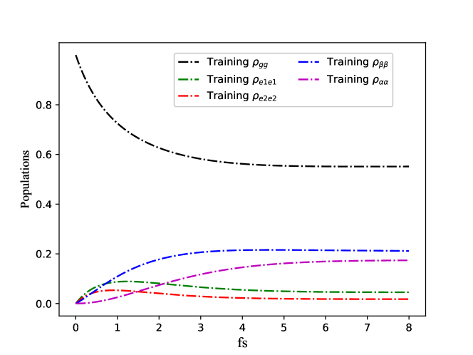
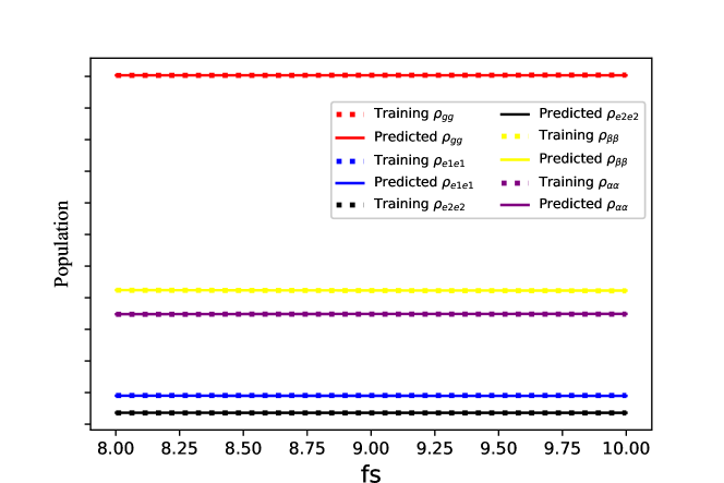
Figure 3: (a) Training models fed by the actual data within [0, 8]fs for populations evolutions in the PSII-RC. (b) Predictive populations compared with the test data set within [8, 10]fs.

The training data set within [0, 8]fs was fed into the proposed LSTM network for learning, and trained by the mentioned approach. Fig.3 (a) shows the populations evolutions in the PSII-RC by the LSTM training model. In order to test the accuracy of the proposed training model, we utilize the trained models to predict the populations evolutions within [8, 10]fs and compare to the test data in the same time domain. The high coincidences shown by the dotted lines and solid lines in Fig.3 (b), demonstrate the accuracy and stability in long term of the proposed LSTM architecture, which is achieved by a series of optimization algorithms mentioned above.

III.2 CT predicted by the LSTM

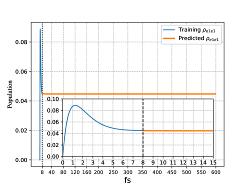
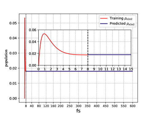
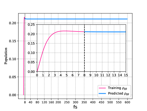
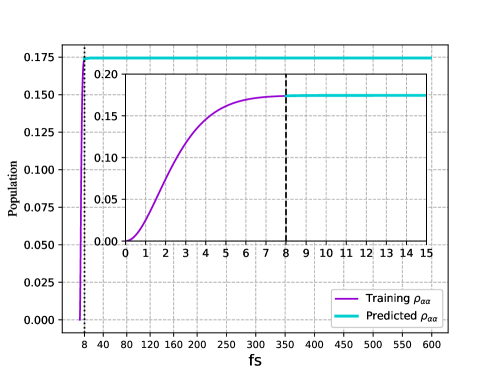
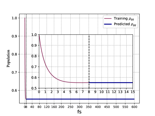
Figure 4: Population evolutions forecasted in [8, 600] fs by the proposed LSTM and training approach.

In this section, our focus is on optimizing predictive performance by fine-tuning neural network hyperparameters, including optimizers, regularization, batch size, learning rate, dropout ratio, and early stopping strategies. In this LSTM model, we employ the Adam optimizer with an initially low learning rate (0.00001) to ensure stable convergence during the training process. Additionally, we have introduced L2 regularization (coefficient of 0.01) and an exceedingly low Dropout ratio (0.0001), aiming to mitigate the risk of overfitting without impairing the model’s learning capacity. By dynamically adjusting the learning rate, our network can adaptively optimize its performance at different stages of training, thereby predicting the CT process more accurately.

Moreover, we expand the short temporal sequence of the training set by a factor of 10 to better capture the training patterns, which is then scaled back by a factor of 10 when invoking the model for a one-shot prediction, returning to the original true scale. Ultimately, we use a single-layer LSTM network with 5-8 neurons, implemented in the TensorFlow framework, to model and predict the CT processdel2021learning . It is noteworthy that after 100 training iterations, the proposed model automatically saves its state if it achieves stability within the specified prediction error threshold of 0.0005. This mechanism significantly enhances training efficiency and reduces unnecessary computational resource consumption(Original codes in “Model training and prediction”).

The experimental results demonstrate that, as training progresses, the model’s performance on the prediction is gradually optimized, proving the effectiveness of the adopted strategies. In particular, through meticulous adjustment of parameters such as batch size and learning rate schedulers, we have observed that the model possesses a commendable generalization ability for CT predictions beyond the training data set. As shown in Fig.4, the vertical black line at 8 fs point demarcates the training data set from the prediction results(Original codes in “Plot figures”). The curves on the right side of the vertical black line correspond to the prediction outcomes obtained by progressively tuning each hyperparameter and optimization strategies. The insert illustrations in Fig.4 enlarge the training and prediction results of our proposed model near 8 fs. The perfect coincidence at 8 fs indicates the accuracy of the model.

Noting that the evolution of all populations over time presents horizontal line distribution (shown in Fig.4) during the whole predictive process, comparing any point taken on the horizontal distribution line can represent the general case. Then, we choose the last actual values obtained from Eq.(10) to compare with the predicted value at 600fs to measure the accuracy of the prediction results, as shown in Table 2. The differences between the actual values and predicted values at 600 fs are all with the $10^{-4}$ orders of magnitude. The negligible difference shows relatively high precision of the prediction model over a long time.

Table 2: Comparison of actual and predicted values at 600 fs.

Populations	Actual value	Predicted value	Difference
$\rho_{e1e1}$	0.04543156	0.04473562	0.00069594
$\rho_{e2e2}$	0.0177977	0.017938	-0.00014031
$\rho_{\alpha\alpha}$	0.17367974	0.17446348	-0.00078374
$\rho_{\beta\beta}$	0.21068688	0.21092759	-0.00024071
$\rho_{gg}$	0.55240412	0.5517195	0.00068464

IV CONCLUSION AND OUTLOOK

In conclusion, the 8000 actual data collected by the Lindblad master equation was fed to the LSTM networks with error threshold training method to predict the charge transport in the Photosystem II (PSII). The error threshold training approach requires that only when the predictions at 10 time points in the test set each had errors below 0.0005, the training model was deemed successfully trained and saved. The prediction results show that LSTM achieved a prediction of $10^{-4}$ magnitude from 8 fs to 600 fs, which effectively enhanced the accuracy of long-term series predictions. The results with precise forecasts, demonstrate the significance of this work in predicting charge transport in PSII, and proper hyperparameter tuning can significantly enhance the accuracy of predictions and the stability of the model. Moreover,this work provides a robust methodological and technical support for future research in the simulation of complex physical processes.

Author contributions

S. C. Zhao conceived the idea. Z. R. Zhao performed the numerical computations and wrote the draft, and S. C. Zhao did the analysis and revised the paper. Y. M. Huang participated in part of the discussion.

V Acknowledgment

This work is supported by the National Natural Science Foundation of China ( Grant Nos. 62065009 and 61565008 ), General Program of Yunnan Applied Basic Research Project, China ( Grant No. 2016FB009 ).

Data Availability Statement

This manuscript has associated data in a data repository.[Authors’ comment: All data included in this manuscript are available upon resonable request by contacting with the corresponding author.] The Supporting Information is available free of charge at: Original codes in Supplement information.

Conflict of Interest

The authors declare that they have no conflict of interest. This article does not contain any studies with human participants or animals performed by any of the authors. Informed consent was obtained from all individual participants included in the study.

References

- (1) H. P. Breuer, E. M. Laine, and J. Piilo. Measure for the degree of non-markovian behavior of quantum processes in open systems. Phys. Rev. Lett., 103(21):210401, 2009.
- (2) V. Bassano, S. Andrea, L. Elsi-Mari, P. Jyrki, and B. Heinz-Peter. Markovianity and non-markovianity in quantum and classical systems. New Journal of Physics, 13(9):093004, 2011.
- (3) F. Shibata, Y. Takahashi, and N. Hashitsume. Reduced dynamics and phenomenological equations of motion for quantum systems in contact with an environment. Journal of Statistical Physics, 17(4):171, 1977.
- (4) . Rivas and S. F. Huelga. Open quantum systems: An introduction. Springer, 2012.
- (5) C. Fleming and B. L. Hu. Perturbation theory for quantum open systems. Annals of Physics, 327(4):1238, 2012.
- (6) A. Strathearn, P. Kirton, D. Kilda, J. Keeling, and B. W. Lovett. High-order perturbative expansion for open quantum systems. Nat. Comm., 9(1):3322, 2018.
- (7) F. Purkayastha and Y. Dubi. Beyond the redfield equation: Modeling environmentally induced dissipation and decoherence in quantum systems. The Journal of Chemical Physics, 154(19):194105, 2021.
- (8) T. M. Stace and S. D. Barrett. Redfield theory for open quantum systems: A perspective on its derivation and application. Phys. Rev. A, 104(2):022217, 2021.
- (9) A. Trushechkin. Redfield equation for weakly coupled open quantum systems: A modified approach. Phys. Rev. A, 103(6):062226, 2021.
- (10) Y. Tanimura. Efficient hierarchical liouville space propagator to quantum dissipative dynamics. The Journal of Chemical Physics, 153(2):020901, 2020.
- (11) M. Wiedmann, J. T. Stockburger, and J. Ankerhold. Modular path integral approach to quantum thermodynamics with hierarchical equations of motion. New J. Physics, 22(3):033007, 2020.
- (12) Z. Tang, X. Ouyang, and J. Cao. Hierarchical equation of motion approach to quantum thermodynamics. The Journal of Chemical Physics, 154(6):064101, 2021.
- (13) A. Erpenbeck and M. Thoss. Hierarchical equations of motion for quantum systems strongly coupled to their environment. The Journal of Chemical Physics, 154(9):094102, 2021.
- (14) Z. Tang and J. Cao. Hybrid stochastic-deterministic approach to the hierarchical equations of motion. The Journal of Chemical Physics, 152(20):204110, 2020.
- (15) H. Wang and M. Thoss. Multi-configurational time-dependent hartree approach to non-markovian dynamics of open quantum systems. The Journal of Chemical Physics, 152(12):124105, 2020.
- (16) M. H. Farag, A. Mandal, and S. Hahn. Multi-configurational time-dependent hartree simulations of singlet fission dynamics in pentacene clusters. The Journal of Physical Chemistry C, 125(8):4732, 2021.
- (17) M. Schrder and A. Chin. Multi-layer multi-configurational time-dependent hartree approach to quantum dynamics of molecules in an explicit solvent environment. The Journal of Chemical Physics, 156(1):014104, 2022.
- (18) A. W. Chin, J. Prior, R. Rosenbach, F. Caycedo-Soler, S. F. Huelga, and M. B. Plenio. Tensor network simulation of non-markovian dynamics in organic polaritons. Phys. Rev. Lett., 124(14):140602, 2020.
- (19) N. Schuch, J. I. Cirac, and F. Verstraete. Convergence and computational complexity of the density matrix renormalization group method. Phys. Rev. B, 100(23):235106, 2019.
- (20) C. Chen, D. Dong, R. Long, I. R. Petersen, and H. A. Rabitz. Overcoming the convergence problem in quantum optimal control with reinforcement learning. Phys. Rev. A, 104(4):042413, 2021.
- (21) J. Schmidt, M. R. G. Marques, S. Botti, and M. A. L. Marques. Machine learning in materials science. npj Computational Materials, 5(1):1–36, 2019.
- (22) D. C. Elton, Z. Boukouvalas, M. D. Fuge, and P. W. Chung. Deep learning for molecular design¡ªa review of the state of the art. Molecular Systems Design & Engineering, 4(4):828, 2019.
- (23) V. Dunjko and H. J. Briegel. Machine learning for quantum technologies. Reports on Progress in Physics, 81(7):074001, 2018.
- (24) M. Ntampaka, H. Trac, D. J. Sutherland, S. Fromenteau, B. P’oczos, and J. Schneider. Machine learning in astronomy and cosmology. The Astronomy and Astrophysics Review, 27(1):1–49, 2019.
- (25) A. M. Palmieri, E. Kovlakov, F. Bianchi, D. Yudin, S. Straupe, J. D. Biamonte, and S. Kulik. Quantum state tomography with neural networks. npj Quantum Information, 6(1):1–8, 2020.
- (26) K. L. Rodrigues, R. Nasser, and S. Pilla. Artificial neural network approach for the evolution of open quantum systems. Phys. Rev. A, 102(4):042408, 2020.
- (27) G. Carleo and M. Troyer. Solving the quantum many-body problem with artificial neural networks. Science, 355(6325):602, 2017.
- (28) G. Zhu, L. Zhang, P. Shen, and J. Song. Long short-term memory networks for time series forecasting. Neurocomputing, 470:80–95, 2022.
- (29) B. Lim and S. Zohren. A review of deep learning for time series forecasting. Machine Learning, 110(11):3079, 2021.
- (30) S. B. Taieb and A. F. Atiya. Forecasting with long short-term memory networks: A review and evaluation. International Journal of Forecasting, 34(4):1044, 2018.
- (31) G. Lai, W. Chang, Y. Yang, and H. Liu. Modeling long-and short-term temporal patterns with deep neural networks. In The 41st International ACM SIGIR Conference on Research and Development in Information Retrieval, page 95, 2018.
- (32) G. Garc’ıa-P’erez, M. A. C. Rossi, B. Sokolov, E. M. Borrelli, and S. Maniscalco. Machine learning non-markovian quantum dynamics with long short-term memory networks. Phys. Rev. Res., 3(2):023084, 2021.
- (33) P. P. Potočnik, L. Knap, and T. Prosen. Forecasting the long-time dynamics of open quantum systems with artificial neural networks. New J. Physics, 24(4):043023, 2022.
- (34) L. F. Li, S. C. Zhao, and L. X. Xu. Charge-transport enhanced by the quantum entanglement in the photosystem II reaction center. European Physical Journal Plus, 136(1050), 2021.
- (35) V. I. Novoderezhkin, E. Romero, J. P. Dekker, and R. V. Grondelle. Multiple charge separation pathways in photosystem II: Modeling of transient absorption kinetics. Chemphyschem A European Journal of Chemical Physics and Physical Chemistry, 12(3):681, 2015.
- (36) M. Qin, H. Z. Shen, X. L. Zhao, and X. X. Yi. Effects of system-bath coupling on a photosynthetic heat engine: A polaron master-equation approach. Phys. Rev. A, 96(1):012125, 2017.
- (37) P. Y. Shi, F. Hou, X. W. Zheng, and F. Yuan. Analysis of electronic health records based on long short-term memory. Concurrency and Computation: Practice and Experience, 32(14):e5684, 2020.
- (38) N. Halpern-Wight, M. Konstantinou, A. G. Charalambides, and A. Reinders. Training and testing of a single-layer lstm network for near-future solar forecasting, 2020.
- (39) H. Wang, W. Y. Zhuang, and X. F. Zhang. Software defect prediction based on gated hierarchical lstms. IEEE Transactions on Reliability, 70(2):711, 2021.
- (40) K. Smagulova, O. Krestinskaya, and A. P. James. A memristor-based long short term memory circuit. Analog Integrated Circuits and Signal Processing, 95:467, 2018.
- (41) A. Kala and S. G. Vaidyanathan. Forecasting monthly rainfall using bio-inspired artificial algae deep learning network. Fluctuation and Noise Letters, 21(02):2250018, 2022.
- (42) K. E. ArunKumar, D. V. Kalaga, C. M. S. Kumar, M. Kawaji, and T. M. Brenza. Forecasting of covid-19 using deep layer recurrent neural networks (rnns) with gated recurrent units (grus) and long short-term memory (lstm) cells. Chaos, Solitons & Fractals, 146:110861, 2021.
- (43) Z. Chang, Y. Zhang, and W. Chen. Electricity price prediction based on hybrid model of adam optimized lstm neural network and wavelet transform. Energy, 187:115804, 2019.
- (44) J. Huang, G. Niu, H. Guan, and S. Song. Ultra-short-term wind power prediction based on lstm with loss shrinkage adam. Energies, 16(9):3789, 2023.
- (45) F. T. Zhou, Z. H. Huang, and C. H. Zhang. Carbon price forecasting based on ceemdan and lstm. Applied energy, 311:118601, 2022.
- (46) Y. Wang. Front-end model of wireless network combined with artificial intelligence in computer information management system. Wireless Communications and Mobile Computing, 2022, 2022.
- (47) Y. Gao, N. Wang, and Y. Ma. L2-ssa-lstm prediction model of steering drilling wellbore trajectory. IEEE Access, 2023.
- (48) J. del Águila Ferrandis, M. S. Triantafyllou, C. Chryssostomidis, and G. E. Karniadakis. Learning functionals via lstm neural networks for predicting vessel dynamics in extreme sea states. Proceedings of the Royal Society A, 477(2245):20190897, 2021.