Optimistic Query Routing in Clustering-based Approximate Maximum Inner Product Search

Abstract

Clustering-based nearest neighbor search is a simple yet effective method in which data points are partitioned into geometric shards to form an index, and only a few shards are searched during query processing to find an approximate set of top-$k$ vectors. Even though the search efficacy is heavily influenced by the algorithm that identifies the set of shards to probe, it has received little attention in the literature. This work attempts to bridge that gap by studying the problem of routing in clustering-based maximum inner product search (MIPS). We begin by unpacking existing routing protocols and notice the surprising contribution of optimism. We then take a page from the sequential decision making literature and formalize that insight following the principle of “optimism in the face of uncertainty.” In particular, we present a new framework that incorporates the moments of the distribution of inner products within each shard to optimistically estimate the maximum inner product. We then present a simple instance of our algorithm that uses only the first two moments to reach the same accuracy as state-of-the-art routers such as Scann by probing up to $50\%$ fewer points on a suite of benchmark MIPS datasets. Our algorithm is also space-efficient: we design a sketch of the second moment whose size is independent of the number of points and in practice requires storing only $O(1)$ additional vectors per shard.

1 Introduction

A fundamental operation in modern information retrieval and database systems is what is known as Nearest Neighbor search or top-$k$ vector retrieval (Bruch, 2024). It is defined as follows: Given a collection $\mathcal{X}$ of $m$ data points in $\operatorname*{\mathbb{R}}^{d}$, we wish to find the $k$ closest points to a query $q\in\operatorname*{\mathbb{R}}^{d}$, where closeness is determined by some notion of vector similarity or distance. In this work, we focus exclusively on inner product as a measure of similarity, leading to the following formal definition known as Maximum Inner Product Search (MIPS):

$$\mathcal{S}=\operatorname*{arg\,max\quad}_{u\in\mathcal{X}}^{(k)}\langle q,u\rangle.$$ (1)

Unsurprisingly, it is often too difficult to solve this problem exactly within a reasonable time budget, especially as $m$ or $d$ increases. As such, the problem is often relaxed to its approximate variant, where we tolerate error in the retrieved set to allow faster query processing. This approximate version of the problem is aptly named Approximate Nearest Neighbor (ANN) search, whose effectiveness is characterized by the fraction of true nearest neighbors recalled in the retrieved set: $\lvert\tilde{\mathcal{S}}\cap\mathcal{S}\rvert/k$, where $\tilde{\mathcal{S}}$ is the set returned by an ANN algorithm.

1.1 Clustering-based ANN search

Algorithms that solve the ANN search problem efficiently and effectively come in various flavors, from trees (Bentley, 1975; Dasgupta and Sinha, 2015), LSH (Indyk and Motwani, 1998), to graphs (Malkov and Yashunin, 2020; Jayaram Subramanya et al., 2019) and more. For a thorough treatment of this subject, we refer the reader to (Bruch, 2024).

The method relevant to this work is the clustering-based approach, also known as Inverted File (IVF) (Jégou et al., 2011), which has proven effective in practice (Auvolat et al., 2015; Babenko and Lempitsky, 2012; Chierichetti et al., 2007; Bruch et al., 2024; Douze et al., 2024). In this paradigm, data points are partitioned into $C$ shards using a clustering function $\zeta:\operatorname*{\mathbb{R}}^{d}\rightarrow[C]$ on $\mathcal{X}$. A typical choice for $\zeta$ is the KMeans algorithm with $C=\mathcal{O}(\sqrt{m})$. This forms the index data structure.

Accompanying the index is a routing function $\tau:\mathbb{R}^{d}\rightarrow[C]^{\ell}$. It takes a query $q$ and returns $\ell$ shards that are more likely to contain its nearest neighbors. A commonly-used router is defined as follows:

$$\tau(q)=\operatorname*{arg\,max\quad}^{(\ell)}_{i\in[C]}\langle q,\mu_{i}\rangle,$$ (2)

where $\mu_{i}$ is the mean of the $i$-th shard.

Processing a query $q$ involves two subroutines. The first stage, which we call “routing,” obtains a list of $\ell$ shards using $\tau(q)$, and the subsequent step, which we refer to as “search,” performs ANN search over the union of the selected shards. While a great deal of research has focused on the latter step (Jégou et al., 2011; Ge et al., 2014; Wu et al., 2017; Andre et al., 2021; Kalantidis and Avrithis, 2014; Johnson et al., 2021; Norouzi and Fleet, 2013), the former step has received relatively little attention. In this work, we turn squarely to the study of the first step: Routing queries to shards.

1.2 The importance of routing

The historical focus on the search step makes a great deal of sense. After all, even though the routing step narrows down the search space, often dramatically so, selected shards may nonetheless contain a large number of points. It is thus imperative that the search stage be efficient and effective.

We argue that the oft-overlooked routing step is important in its own right. The first and obvious reason is that, the more accurately a router chooses a subset of shards, the fewer data points the search stage must examine. For example, if shards are balanced in size, access to an oracle router means that the search stage need only examine $m/C$ points to find the top-$1$ point.

The second and more important reason pertains to scale. As collections grow in size and dimensionality, it is often infeasible to keep the entire index in memory, in spite of advanced compression techniques such as Product Quantization (Jégou et al., 2011). Much of the index must therefore rest on secondary storage—in particular, cheap but high-latency storage such as disk or blob storage—and accessed only when necessary. That line of reasoning has led to the emergence of disk-based graph indexes (Jayaram Subramanya et al., 2019; Singh et al., 2021; Jaiswal et al., 2022) and the like.

Translating the same rationale to the clustering-based paradigm implies that shards rest outside of the main memory, and that when a router identifies a subset of shards, the search stage must fetch those shards from storage for further processing. A more accurate router thus lowers the volume of data that must be transferred between storage and memory. Furthermore, because query processing is additionally bottlenecked by storage bandwidth and memory capacity, fetching fewer shards per query is a requisite for achieving a higher throughput.

Interestingly, depending on operational factors such as query load, storage I/O bandwidth, data transfer rate, and memory utilization, it would be acceptable for the routing stage to be more computationally expensive as long as it identifies shards more accurately. Whereas the in-memory clustering-based paradigm requires routing to be highly efficient, the new trade-off space offered by its storage-based realization opens the door to more nuanced research.

1.3 Existing routers and the surprising role of optimism

We have argued that routing accuracy is increasingly relevant. Surprisingly, with the exception of one recent work that explores supervised learning-to-rank for routing (Vecchiato et al., 2024), the few existing unsupervised routers take the naïve form of Equation (2). In effect, they determine the relative potential “reward” of every shard with a point estimate.

Take Equation (2) as the most prominent example. What we refer to as the Mean router summarizes each shard with its mean point (i.e., $\mu_{i}$ for shard $i$). This is not an unreasonable choice as the mean is the minimizer of the variance, and is, in fact, natural if KMeans is the clustering algorithm $\zeta$.

Another common router, which we call NormalizedMean, belongs to the same family, but where shard representatives are the $L_{2}$-normalized means, rather than the unnormalized mean vectors:

$$\tau(q)=\operatorname*{arg\,max\quad}^{(\ell)}_{i\in[C]}\langle q,\frac{\mu_{i}}{\lVert\mu_{i}\rVert_{2}}\rangle.$$ (3)

This formulation is inherited from the familiar Spherical KMeans (Dhillon and Modha, 2001), which is identical to the standard KMeans iterative algorithm but, at the end of every iteration, cluster centroids are projected onto the unit sphere. Because we can assume that $\lVert q\rVert_{2}=1$ without loss of generality, it is easy to see that Equation (3) routes by the angle between $q$ and the mean vectors.

Intuitively, NormalizedMean seems appropriate for ANN search over a sphere: When norms do not affect the outcome of ANN search, then all that matters in Equation (1) is the angle between $q$ and data points, rendering it reasonable to rank shards by the angle between their mean and $q$.

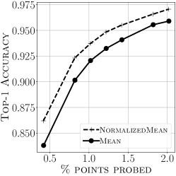
(a)

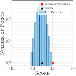
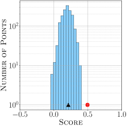
(b)

Figure 1: (a) Top-$1$ recall versus the number of points probed on the Text2Image dataset where data points have varying norms; (b) Distribution of inner products between a shard and a sample query on GloVe. Overlaid are the scores computed by Mean and NormalizedMean routers.

Intriguingly, in many circumstances that deviate from that situation, NormalizedMean tends to perform more accurately than the Mean router, as evidenced in Figure LABEL:sub@figure:motivation:mean_vs_normalized_mean. Because unpacking this phenomenon motivates our proposal, we take a brief moment to take a closer look.

Consider a query point $q$ and a single shard $\mathcal{P}$ with mean $\mu$. We visualize in Figure LABEL:sub@figure:motivation:score_distribution the distribution of inner products between $q$ and every point in $\mathcal{P}$. Overlaid with that distribution is the inner product between $q$ and the mean of points in $\mathcal{P}$, as well as their normalized mean. We observe that $\langle q,\mu/\lVert\mu\rVert_{2}\rangle$ lands in the right tail of the distribution.

That is not surprising, at least for the case where $\lVert u\rVert_{2}=1$ for all $u\in\mathcal{P}$. Clearly $\lVert\mu\rVert_{2}\leq 1$, so that $\langle q,\mu/\lVert\mu\rVert_{2}\rangle=\langle q,\mu\rangle/\lVert\mu\rVert_{2}\geq\langle q,\mu\rangle$; the NormalizedMean router amplifies the Mean router by a factor of $1/\lVert\mu\rVert_{2}$. What is interesting, however, is that the magnitude of this “boost” correlates with the variance of the data points within $\mathcal{P}$: The more concentrated $\mathcal{P}$ is around the direction of its mean, the closer the mean is to the surface of the sphere, so that NormalizedMean applies a smaller amplification to $\langle q,\mu\rangle$. The opposite is true when points are spread out. As a result, shards with a higher variance receive a larger lift by the NormalizedMean router!

This has its downsides. First, it is hard to explain the behavior on point sets with varying norms. Second, as we observe in Figure LABEL:sub@figure:motivation:score_distribution, NormalizedMean aggressively overestimates. Nonetheless, the insight that a router’s score for a shard can be influenced by the shard’s variance is worth exploring.

We can summarize our observation as follows. The estimate given by the NormalizedMean router paints an optimistic picture of what the maximum inner product between $q$ and points in $\mathcal{P}$ could be. Contrast that with the Mean router, which is naturally a conservative estimate.

This work investigates the ramifications of that insight. In particular, the research question we wish to study is whether a more principled approach to designing optimistic routers can lead to more accurate routing decisions on vector sets with variable norms. The nature of this question is not unlike those asked in the online learning literature (Lattimore and Szepesvári, 2020), so it is not surprising that our answer to this question draws from the “principle of optimism in the face of uncertainty.”

1.4 Contributions and outline

We apply the Optimism Principle to routing in clustering-based MIPS. Our formulation, presented in Section 2, rests on the concentration of the inner product distribution between a query $q$ and a set of points in the same shard. In particular, we estimate a score, $\theta_{i}$, for the $i$-th shard such that, with some confidence, the maximum inner product of $q$ with points in that shard is at most $\theta_{i}$. Shards are then ranked by their score for routing. Notice that, when $\theta_{i}=\mu_{i}$, we recover the Mean router, and when $\theta_{i}>\mu_{i}$ routing is optimistic with the confidence parameter determining the degree of optimism.

Building on our proposed formalism of an optimistic router, we outline a general framework that can incorporate as much information as is available about the data distribution to estimate the aforementioned scores. We then present a concrete, assumption-free instance of our algorithm that uses the first and second moments of the empirical inner product distribution only. Furthermore, we make the resulting algorithm space-efficient by designing a sketch (Woodruff, 2014) of the second moment. The end-result is a practical algorithm that is straightforward to implement.

We put our proposal to the test in Section 3 on a variety of ANN benchmark datasets. As our experiments show, our optimistic router achieves the same ANN recall as state-of-the-art routers but with up to a $50\%$ reduction in the total number of data points evaluated per query. We conclude this work in Section 4.

2 Routing by the Optimism Principle: our proposal

As we observed, NormalizedMean is an optimistic estimator, though its behavior is unpredictable. Our goal is to design an optimistic estimator that is statistically principled, thus well-behaved.

Before we begin, let us briefly comment on our terminology and notation. Throughout this section, we fix a unit query vector $q$; all discussions are in the context of $q$. We denote the $i$-th shard by $\mathcal{P}_{i}$, and write $S_{i}$ for the set of inner product scores between $q$ and points in $\mathcal{P}_{i}$: $S_{i}=\{\langle q,u\rangle:u\in\mathcal{P}_{i}\}$.

2.1 Formalizing the notion of optimism

We wish to find the smallest threshold $\theta_{i}\geq\langle q,\mu_{i}\rangle$ for the $i$-th shard such that the probability that a sample from $S_{i}$ falls to the left of $\theta_{i}$ is at least $(1+\delta)/2$, for some arbitrary $\delta\in[0,1]$. Formally, we aim to compute a solution $\theta_{i}$ to the the following optimization problem:

Problem 1 (Optimistic estimator of the maximum inner product in $S_{i}$).

$$\inf\{\theta_{i}:\theta_{i}\geq\langle q,\mu_{i}\rangle\}\quad\text{ such that }\Pr_{s\sim S_{i}}[s\leq\theta_{i}]\geq\frac{1+\delta}{2}.$$

One can interpret the optimal $\theta_{i}$ as a probabilistic upper-bound on the maximum attainable value in $S_{i}$; that is, with some confidence, we can assert that no value in $S_{i}$ is greater than $\theta_{i}$.

Equipped with $\theta_{i}$’s, we route $q$ by sorting all shards by their estimated thresholds in descending order and subsequently selecting the top shards in the resulting ranked list. Our router, dubbed Optimist, is defined as follow:

$$\tau(q)=\operatorname*{arg\,max\quad}^{(\ell)}_{i\in[C]}\theta_{i}.$$ (4)

2.2 Understanding the routing behavior

Suppose for a moment that we have the solution to Problem 1, and let us expand on the expected behavior of the Optimist router. It is easy to see that, when $\delta\rightarrow 0$, the optimal solution approaches $\theta_{i}=\langle q,\mu_{i}\rangle$. As such, if we wish to obtain the most conservative estimate of the maximum inner product between $q$ and points in $\mathcal{P}_{i}$, the routing procedure collapses to the Mean router.

As $\delta\rightarrow 1$, $\theta_{i}$ becomes larger, rendering Equation (4) an enthusiastically optimistic router. At the extreme, the optimal solution is the maximum inner product itself.

Clearly then, $\delta$ controls the amount of optimism one bestows onto the router. It is interesting to note that, when the data distribution is fully known, then $\delta=1$ is an appropriate choice: If we know the exact distribution, we can expect to be fully confident about the maximum inner product. On the other hand, when very little about the distribution is known (e.g., when all we know is the first moment of the distribution), then $\delta=0$ is a sensible choice. In effect, the value of $\delta$ is a statement on our knowledge of the underlying data distribution.

What is left to address is the solution to Problem 1, which is the topic of the remainder of this section. We defer a description of a general approach that uses as much or as little information as available about the data distribution to Appendix B due to space constraints. In the next section, we present a more practical approach that is the foundation of the rest of this work.

2.3 Practical solution via concentration inequalities and sketching

Noting that Problem 1 is captured by the concept of concentration of measure, we resort to results from that literature to find acceptable estimates of $\theta_{i}$’s. In particular, we obtain a solution via a straightforward application of the one-sided Chebyshev’s inequality, resulting in the following lemma.

Lemma 1.

Denote by $\mu_{i}$ and $\Sigma_{i}$ the mean and covariance of the distribution of $\mathcal{P}_{i}$. An upper-bound on the solution to Problem 1 for $\delta\in(0,1)$ is:

$$\theta_{i}=\langle q,\mu_{i}\rangle+\sqrt{\frac{1+\delta}{1-\delta}\;q^{\top}\Sigma_{i}q}.$$ (5)

Proof.

The result follows immediately by applying the one-sided Chebyshev’s inequality to the distribution, $S_{i}$, of inner products between $q$ and points in $\mathcal{P}_{i}$:

$$\Pr_{s\sim S_{i}}[s-\langle q,\mu_{i}\rangle\leq\epsilon]\geq 1-\frac{q^{\top}\Sigma_{i}q}{q^{\top}\Sigma_{i}q+\epsilon^{2}}=\frac{1+\delta}{2}\implies\epsilon^{2}=\frac{1+\delta}{1-\delta}\;q^{\top}\Sigma_{i}q.$$

Rearranging the terms to match the expression of Problem 1 gives $\theta_{i}=\langle q,\mu_{i}\rangle+\epsilon$, as desired. ∎

We emphasize that the solution obtained by Lemma 1 is not necessarily optimal for Problem 1. Instead, it gives the best upper-bound on the optimal value of $\theta_{i}$ that can be obtained given limited information about the data distribution. As we see later, however, even this sub-optimal solution proves effective in practice.

Approximating the covariance matrix.

While Equation (5) gives us an algorithm to approximate the threshold $\theta_{i}$, storing $\Sigma_{i}$ can be prohibitive in practice. That is because the size of the matrix grows as $d^{2}$ for each partition. Contrast that with the cost for other routers, such as Mean and NormalizedMean, which only store a single $d$-dimensional vector per partition. To remedy this inefficiency, we reduce the cost of representing $\Sigma_{i}$ by storing a small sketch that approximates it.

Since the procedure we describe is independently applied to each partition, we drop the subscript for $\Sigma_{i}$ and describe the procedure for a single partition. We seek a matrix $\tilde{\Sigma}\in\operatorname*{\mathbb{R}}^{d\times d}$ that approximates $\Sigma$. We define the approximation error as follows:

$$\text{err}(\Sigma,\tilde{\Sigma})=\sup_{\begin{subarray}{c}\|v\|_{2}=1\end{subarray}}|v^{\top}\Sigma v-v^{\top}\tilde{\Sigma}v|.$$

A standard mechanism to approximate large matrices in order to minimize this error is to compute a low-rank approximation of the original matrix. To that end, let $\Sigma=V\Lambda V^{\top}$ be the eigendecomposition of the positive semi-definite matrix $\Sigma$; where the columns of $V$ contain the orthonormal eigenvectors of $\Sigma$ and $\Lambda$, a $d\times d$ diagonal matrix, contains the non-negative eigenvalues of $\Sigma$ in non-increasing order. The Eckhart-Young-Mirsky Theorem shows that

$$\text{err}_{t}(\Sigma)=\inf_{\begin{subarray}{c}\tilde{\Sigma}\in\operatorname*{\mathbb{R}}^{d\times d}\ \text{s.t. rank}(\tilde{\Sigma})=t\end{subarray}}\text{err}(\Sigma,\tilde{\Sigma}),$$ (6)

is minimized when $\tilde{\Sigma}=[V\sqrt{\Lambda}]_{t}[V\sqrt{\Lambda}]_{t}^{\top}$, where $[\cdot]_{t}$ corresponds to the operator that selects the first $t$ columns of the matrix.

While (6) is a well-known fact, in practice, it is often the case that the diagonal of the matrix $\Sigma$ contains important information and preserving it fully leads to better approximations of the matrix. As such, we decompose $\Sigma$ as a sum of two matrices: $D$ a diagonal matrix containing the diagonal entries of $\Sigma$, and the residual $R=\Sigma-D$. We preserve the diagonal $D$ fully and approximate $R$ by computing a low-rank approximation of a symmetrization of $R$. Specifically, we decompose

$$\Sigma=D+R=D^{\frac{1}{2}}(I+D^{-\frac{1}{2}}RD^{-\frac{1}{2}})D^{\frac{1}{2}},$$

and compute a low-rank approximation to $M=D^{-\frac{1}{2}}RD^{-\frac{1}{2}}$. Notice that since $M$ is a symmetric real-valued matrix, it has an eigendecomposition of the form $M=Q\Lambda Q^{\top}$ where $Q$ is a $d\times d$ matrix with orthonormal columns (corresponding to the eigenvectors of $M$) and $\Lambda$ is a $d\times d$ diagonal matrix containing the (possibly negative) eigenvalues of $M$ along the diagonal. Given some target sketch size $t\leq d$, we sketch $\Sigma$ as:

$$\tilde{\Sigma}=D+D^{\frac{1}{2}}[Q]_{t}[\Lambda]_{t}[Q]_{t}^{\top}D^{\frac{1}{2}}.$$ (7)

While this is not a standard mechanism to sketch PSD matrices and can in the worst case perform worse than the “optimal” low-rank sketch, we show that under certain practical assumptions, this sketch can have error lower than that of standard low-rank approximation.

Lemma 2.

Let $\Sigma\in\operatorname*{\mathbb{R}}^{d\times d}$ be a PSD matrix with diagonal $D$ and the property that $\min_{i\in[d]}{D_{ii}}/{\max_{j\in[d]}D_{jj}}\geq 1-\epsilon$ for some $\epsilon>0$. For every $1\leq t\leq d-1$ such that the $(t+1)$-st eigenvalue of $D^{-1/2}\Sigma D^{-1/2}$ is greater than $2$, the sketch $\tilde{\Sigma}$ defined in (7) has the property that $\text{err}(\Sigma,\tilde{\Sigma})\leq\text{err}_{t}(\Sigma)\cdot\frac{1}{1-\epsilon}$.

We provide a proof for the above result in Appendix C and show that for practical datasets, including the ones we use in this work, the assumptions in the lemma are valid.

2.4 The final algorithm

Using our solution from Lemma 1 for Problem 1 and our sketch defined in (7), we describe our full algorithm in Algorithm 1 for building our router and scoring a partition for a given query. Notice that, since we only store $\mu,D,[\Lambda]_{t}$ and $[Q]_{t}$, the router requires just $t+2$ vectors in $\operatorname*{\mathbb{R}}^{d}$ per partition. In our experiments, we choose $t\leq 10$ for all datasets except one and show that much of the performance gains from using the whole covariance matrix can be preserved even by choosing a small value of $t$ independent of $d$.

Algorithm 1 Indexing and scoring a single partition with Optimist

1:Set of $n$ points $\mathcal{X}=x_{1},\dots,x_{n}$ defining the partition and target rank $t$ such that $t\leq d$.

2:procedure BuildRouter($\mathcal{X},t$)

3:     Compute and store $\mu\leftarrow\frac{1}{n}\sum_{i=1}^{n}x_{i}$.

4:     Compute $\Sigma\leftarrow\frac{1}{n}\sum_{i=1}^{n}(x_{i}-\mu)(x_{i}-\mu)^{\top}$. $\triangleright$ This does not need to be stored

5:     Decompose $\Sigma$ into diagonal $D$ and residual $R$ $\triangleright$ $\Sigma=D+R$

6:     Compute eigendecomposition of $D^{-1/2}RD^{-1/2}=Q\Lambda Q^{\top}$

7:     Sort columns of $Q$, $\Lambda$ in non-increasing order.

8:     Store $D$, $\Lambda_{t}\leftarrow[\Lambda]_{t}$ and $Q_{t}\leftarrow[Q]_{t}$

9:Query $q\in\operatorname*{\mathbb{R}}^{d}$ and confidence parameter $\delta>0$.

10:procedure Score($q,\delta$)

11:     Compute $\tilde{q}\leftarrow q\circ D^{1/2}$ $\triangleright$ Element-wise product with diagonal of $D^{1/2}$

12:     return $\langle q,\mu\rangle+\sqrt{\frac{1+\delta}{1-\delta}\cdot(\|\tilde{q}\|_{2}^{2}+\tilde{q}^{\top}Q_{t}\Lambda_{t}Q_{t}^{\top}\tilde{q})}$

3 Experimental evaluation

In this section, we put our arguments to the test and experimentally evaluate Optimist.

3.1 Setup

Datasets: We use the following suite of benchmark ANN datasets: Text2Image ($10$ million points, $d=200$); Music ($1$m, $d=100$); DeepImage ($10$m, $d=96$); GloVe ($1{.}2$m, $d=200$); MsMarco-MiniLM ($8{.}8$m, $d=384$); and, Nq-Ada2 ($2.7$m, $d=1{,}536$). We defer a complete description of these datasets to Appendix A due to space constraints.

Clustering: For our main results, we partition datasets with Spherical KMeans (Dhillon and Modha, 2001). We include in the appendix results from similar experiments but where the clustering algorithm is standard KMeans and Gaussian Mixture Model (GMM). We cluster each dataset into $\sqrt{m}$ shards, where $m$ is the number of data points in the dataset.

Evaluation: Once a dataset is partitioned, we evaluate a router $\tau$ as follows. For each test query, we identify the set of shards to probe using $\tau$. We then perform exact search over the selected shards, obtain the top-$k$ points, and compute recall with respect to the exact top-$k$ set. Because the only source of error is the inaccuracy of the router, the measured recall gauges the effectiveness of $\tau$.

We report recall as a function of the number of data points probed, rather than the number of shards probed. In this way, a comparison of the efficacy of different routers is unaffected by any imbalance in shard sizes, so that a router cannot trivially outperform another by simply prioritizing larger shards.

Figure 2: Top-$k$ recall on Nq-Ada2 versus the number of probed data points. The dataset is partitioned with Spherical KMeans. Scann has parameter $T$, SubPartition $t$ (leading to $t+2$ sub-partitions per shard), and Optimist rank $t$ and degree of optimism $\delta$.

Routers: We evaluate the following routers in our experiments:

• Mean and NormalizedMean: Defined in Equations (2) and (3), respectively;

• Scann $(T)$: Similar to Mean and NormalizedMean, but where routing is determined by inner product between a query and the Scann centroids (c.f., Theorem $4{.}2$ in (Guo et al., 2020)). Scann has a single hyperparameter $T$, which we set to $0.5$ after tuning;

• SubPartition $(t)$: Recall that Optimist stores $t+2$ vectors per partition, where $t$ is the rank in Equation (7). We ask if simply partitioning each shard independently into $t+2$ sub-partitions, and recording the sub-partitions’ centroids as the representatives of that shard attains the same routing accuracy as Optimist. At query time, we take the maximum inner product of the query with a shard’s representatives as its score, and sort shards according to this score; and,

• Optimist $(t,\delta)$: The Optimist router given in Algorithm 1. The parameter $t$ determines the rank of the sketch of the covariance matrix, and $\delta$ determines the degree of optimism. We set $t$ to a maximum of $2\%$ of $d$ but study its effect in Appendix E. $t=d$ indicates that the full covariance matrix is used (i.e., without sketching).

Code: We have implemented all baseline and proposed routers in the Rust programming language. We intend to open-source our code along with experimental configuration to facilitate reproducibility.

3.2 Main results

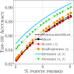
(a) GloVe

(b) MsMarco-MiniLM

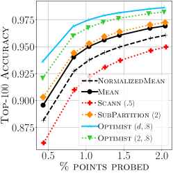
(c) Music

Figure 3: Top-$100$ recall versus the number of probed data points. Setup is the same as Figure 2.

Figure 2 plots top-$k$ recall for $k\in\{1,10,100\}$ versus the percentage of data points examined for Nq-Ada2—Appendix D.1 gives full results for all datasets. Note that, partitioning is by Spherical KMeans, with similar plots for standard KMeans in Appendix D.2 and GMM in Appendix D.3.

We summarize a few key observations. First, among baselines, NormalizedMean generally outperforms Mean and Scann, save for Music where Mean reaches a higher recall. Second, with very few exceptions, Optimist with the full covariance (i.e., $t=d$) does at least as well as NormalizedMean, and often outperforms it significantly. Interestingly, the gap between baselines and Optimist widens as retrieval depth ($k$) increases; a phenomenon that is not surprising.

Finally, while Optimist with $t\ll d$ shows some degradation with respect to the $t=d$ configuration—as anticipated—it still achieves a higher recall than baselines for larger $k$. When $k$ is smaller, the SubPartition router with $t+2$ vectors becomes a strong competitor.

We highlight that, Optimist shines when data points are not on the surface of a sphere (or concentrated close to it). This phenomenon is illustrated in Figure 3, showing top-$100$ recall for a subset of datasets partitioned with Spherical KMeans—refer to Appendix D for results on other datasets.

In particular, on Music, at $95\%$ top-$100$ recall, Optimist with $t\ll d$ needs to probe $54\%$ fewer data points than NormalizedMean; on average Optimist probes $6{,}666$ data points to reach $95\%$ top-$100$ recall whereas NormalizedMean examines $14{,}463$ points. We present the relative savings on all datasets in Table 1. Note that, on DeepImage, no method outperforms NormalizedMean.

Table 1: The relative savings in amount of data probed between Optimist $(t\ll d,.8)$ and NormalizedMean to achieve a fixed recall. A saving of $x\%$ means that Optimist scans $x\%$ fewer data points than NormalizedMean for the same recall.

Recall	Nq-Ada2	GloVe	MsMarco-MiniLM	DeepImage	Music	Text2Image
$90\%$	$18\%$	$11\%$	$22\%$	$0$	$38\%$	$23\%$
$95\%$	$20\%$	$5.5\%$	$7.7\%$	$0$	$54\%$	$22\%$

We conclude this section by noting that, in Appendix E, we study the effect of $t$ and $\delta$ on the performance of Optimist. We exclude the full discussion from the main prose due to space constraints, but mention that the observations are unsurprising.

3.3 Maximum inner product prediction

We claimed that Optimist is statistically principled. That entails that Optimist should give a more accurate estimate of what the maximum inner product can be for any given query-partition pair. We examine that claim in this section and quantify the prediction error for all routers.

Fix a dataset, whose $C$ partitions are denoted by $\mathcal{P}_{i}$ for $i\in[C]$, along with a router $\tau$ and query $q$. We write $\tau_{i}$ to denote the score computed by $\tau$ for partition $\mathcal{P}_{i}$ and $q$ (e.g., NormalizedMean computes $\langle q,\mu_{i}/\lVert\mu_{i}\rVert_{2}\rangle$ and Optimist gives $\theta_{i}$ per Problem 1).

Note that, the $\tau_{i}$’s induce an ordering among partitions. We denote this permutation by $\pi$, so that $\tau_{\pi_{i}}\geq\tau_{\pi_{i+1}}$. We quantify the prediction error for $\ell\in[C]$ as:

$$\mathcal{E}_{\ell}(\tau,q)=\frac{1}{\ell}\sum_{i=1}^{\ell}\left|\frac{\tau_{\pi_{i}}}{\max_{u\in\mathcal{P}_{\pi_{i}}}\langle q,u\rangle}-1\right|.$$ (8)

This error is $0$ when scores produced by the router perfectly match the maximum inner product. The role of $\ell$ is to allow us to factor in the rank of partitions in our characterization of the prediction error. In other words, we can measure the error only for the top $\ell$ shards according to $\tau$. In this way, if we decide that it is not imperative for a router to accurately predict the maximum inner product in low-ranking shards, we can reflect that choice in our calculation.

We measure Equation (8) on all datasets partitioned by Spherical KMeans, and all routers considered in this work. The results are shown in Figure 4, with the remaining datasets in Appendix F, where for each choice of $\ell$, we plot $\mathbb{E}_{q}[\mathcal{E}_{\ell}(\tau,q)]$ using the test query distribution.

From the figures, with the exception of Scann on Text2Image, it is clear that all routers suffer a greater error as $\ell\rightarrow C$ (i.e., $\%$ shards approaches $100\%$). Interestingly, $\textsc{Optimist}(t=d,\cdot)$ degrades much less severely. Remarkably, when $t\ll d$, the same pattern persists; Music excepted, where, with $t=2$, Optimist becomes highly inaccurate when $\ell\geq 8\%$ of the total number of shards.

(a) GloVe

(b) MsMarco-MiniLM

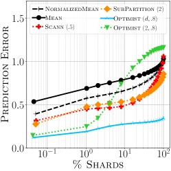
(c) Music

Figure 4: Mean prediction error of Equation (8) vs. $\ell$ (percent of total number of shards, $\log$-scale).

4 Concluding remarks

Motivated by our observation that NormalizedMean is an over-estimator of maximum inner product, we formalized the notion of optimism for query routing in clustering-based MIPS and presented a principled optimistic algorithm that estimates the maximum inner product with much greater accuracy and exhibits a more reliable behavior. Results on a suite of benchmark datasets confirm our claims.

We highlight that our algorithm is more suitable for settings where individual shards rest on some external, high-latency storage, so that spending more compute on routing can be tolerated in exchange for fewer amount of data transferred between storage and main memory.

We leave to future work an exploration of a more compact sketching of the covariance matrix; and, an efficient realization of our general solution outlined in Appendix B.

Appendix A Description of datasets

We use the following benchmark datasets in this work:

• Text2Image: A cross-modal dataset, where data and query points may have different distributions in a shared space [Simhadri et al., 2022]. We use a subset consisting of $10$ million $200$-dimensional data points along with a subset of $10{,}000$ test queries;

• Music: $1$ million $100$-dimensional points [Morozov and Babenko, 2018] with $1{,}000$ queries;

• DeepImage: A subset of $10$ million $96$-dimensional points from the billion deep image features dataset [Yandex and Lempitsky, 2016] with $10{,}000$ test queries;

• GloVe: $1{.}2$ million, $200$-dimensional word embeddings trained on tweets [Pennington et al., 2014] with $10{,}000$ test queries;

• MsMarco-MiniLM: Ms Marco Passage Retrieval v1 [Nguyen et al., 2016] is a question-answering dataset consisting of $8{.}8$ million short passages in English. We use the “dev” set of queries for retrieval, made up of $6{,}980$ questions. We embed individual passages and queries using the all-MiniLM-L6-v2 model to form a $384$-dimensional vector collection; and,

• Nq-Ada2: $2{.}7$ million, $1{,}536$-dimensional embeddings of the Nq natural questions dataset [Kwiatkowski et al., 2019] with the Ada-002 model.

We note that the last four datasets are intended for cosine similarity search. As such we normalize these collections prior to indexing, reducing the task to MIPS of Equation (1).

Appendix B General solution

Let $\mathcal{D}$ be an unknown distribution over $\operatorname*{\mathbb{R}}^{d}$ from which shard $\mathcal{P}_{i}$ is sampled. It is clear that, if we are able to accurately approximate the quantiles of $S_{i}$, we can obtain an estimate $\theta_{i}$ satisfying Problem 1.

Let us motivate our approach by considering a special case where $\mathcal{D}$ is $\mathcal{N}(\mu_{i},\Sigma_{i})$, a Gaussian with mean $\mu_{i}\in\operatorname*{\mathbb{R}}^{d}$ and covariance $\Sigma_{i}\in\operatorname*{\mathbb{R}}^{d\times d}$. In this case, $S_{i}$ follows a univariate Gaussian distribution with mean $\langle q,\mu_{i}\rangle$ and variance $q^{\top}\Sigma_{i}q$. In this setup, a solution to Problem 1 is simply:

$$\theta_{i}=\langle q,\mu_{i}\rangle+\sqrt{q^{\top}\Sigma_{i}q}\cdot\Phi_{\mathcal{N}(0,1)}^{-1}\left(\frac{1+\delta}{2}\right),$$ (9)

which follows by expressing the cumulative distribution function (CDF) of $S_{i}$ in terms of the CDF of a unit Gaussian, denoted by $\Phi_{\mathcal{N}(0,1)}$.

Notice in the above example that, we first modeled the moments of $S_{i}$ using the moments of $\mathcal{D}$. We then approximated the CDF (or equivalently, the quantile function) of the distribution of $S_{i}$ using its moments—in the Gaussian case, the approximation with the first two moments is, in fact, exact.

Our general solution follows that same logic. In the first step, we can obtain the first $r$ moments of the distribution of $S_{i}$, denoted by $m_{j}(S_{i})$ for $j\in[r]$, from the moments of $\mathcal{D}$, denoted by $m_{j}(\mathcal{D})$. In a subsequent step, we use $m_{j}(S_{i})$’s to approximate the CDF of $S_{i}$.

It is easy to see that the $j$-th moment of $S_{i}$ can be written as follows:

$$m_{j}(S_{i})=q^{\otimes j}\odot m_{j}(\mathcal{D})\approx\frac{1}{n}\cdot q^{\otimes j}\odot\sum_{u_{1},\dots,u_{n}\sim\mathcal{D}}x^{\otimes j},$$

where ^⊗j is the $j$-fold tensor product, and $\odot$ tensor inner product.

In our second step, we wish to find a distribution $\tilde{S}_{i}$ such that $m_{j}(\tilde{S}_{i})\approx m_{j}(S_{i})$ for all $j\in[r]$. This can be done using the “method of moments,” a classic technique in statistics Pearson [1936] that offers guarantees [Kong and Valiant, 2017, Braverman et al., 2022] in terms of a distributional distance such as the Wasserstein-1 distance.

While using higher-order moments can lead to a better approximation, computing the $j$-th moment for $j>2$ can be highly expensive considering the dimensionality of datasets seen in practice, as the memory requirement to store the tensor $m_{j}(\mathcal{D})$ grows as $d^{j}$. Hence, we leave exploration and design of an efficient version of this two-step approach as future work.

Appendix C Sketching the covariance matrix

Let $\Sigma=D+R$ be the decomposition of the PSD covariance matrix $\Sigma$ into its diagonal $D$ and residual $R=\Sigma-D$. Let $Q\Lambda Q^{\top}$ be the orthogonal eigendecomposition of $D^{-1/2}RD^{-1/2}$. Recall that we define $\tilde{\Sigma}$, the sketch, for some $1\leq t\leq d$ as

$$\tilde{\Sigma}:=D+D^{{1}/{2}}[Q]_{t}[\Lambda]_{t}[Q]_{t}^{\top}D^{{1}/{2}}$$

We start by providing a proof for Lemma 2 given the assumptions in the lemma are true; i.e. the $(t+1)$-th eigenvalue of $D^{-1/2}\Sigma D^{-1/2}$ is greater than or equal to $2$ and $\min_{i\in[d]}\Sigma_{ii}/\max_{j\in[d]}\Sigma_{jj}\geq(1-\epsilon)$ for some $0\leq\epsilon<1$. We then proceed to justify these assumptions in the following section.

C.1 Proof of Lemma 2

First, we state three facts that we will use to simplify our proof for Lemma 2.

Fact 1.

For any symmetric matrix $M\in\operatorname*{\mathbb{R}}^{d\times d}$ with eigendecomposition $USU^{\top}$, we have that for any $v\in\operatorname*{\mathbb{R}}^{d}$,

$$v^{\top}Mv=\sum_{i=1}^{d}S_{i}\cdot\langle v,U_{i}\rangle^{2}.$$

Fact 2.

Assuming the eigenvalues $\Lambda$ of $D^{-1/2}RD^{-1/2}$ are sorted in non-increasing order, we have that $I+D^{-1/2}RD^{-1/2}=Q(I+\Lambda)Q^{\top}$. In words, the eigenvectors of $I+D^{-1/2}RD^{-1/2}$ are the same as $D^{-1/2}RD^{-1/2}$ and the $i$-th eigenvalue is $\Lambda_{i}+1$.

As a corollary, since $I+D^{-1/2}RD^{-1/2}$ is positive semidefinite, we have that $\Lambda_{i}\geq-1$ for all $i\in[d]$.

Proof.

This follows easily after noticing that $I=QQ^{\top}$ because $Q$ is a $d\times d$ matrix with orthonormal columns (and rows). ∎

Fact 3.

For a diagonal matrix $S\in\operatorname*{\mathbb{R}}^{d\times d}$ with bounded positive entries, i.e. $0<l\leq S_{ii}\leq u$ for all $i\in[d]$, and arbitrary vector $v\in\operatorname*{\mathbb{R}}^{d}$, we have that $l\|v\|_{2}\leq\|Sv\|_{2}\leq u\|v\|_{2}$.

Now we are ready to prove the lemma. For any arbitrary vector $v\in\operatorname*{\mathbb{R}}^{d}$ we have that

$$v^{\top}(D^{-\frac{1}{2}}\Sigma D^{-\frac{1}{2}}-D^{-\frac{1}{2}}\tilde{\Sigma}D^{-\frac{1}{2}})v =v^{\top}(D^{-\frac{1}{2}}RD^{-\frac{1}{2}}-[Q]_{t}[\Lambda]_{t}[Q]_{t}^{\top})v$$ (10)

$$=\sum_{i=t+1}^{d}\Lambda_{i}\cdot\langle Q_{i},v\rangle^{2}$$ (11)

where the first equality follows by the definition of $\tilde{\Sigma}$ and the second by Fact 1. Hence, by the definition of $\text{err}(\cdot,\cdot)$, we have that $\text{err}(D^{-\frac{1}{2}}\Sigma D^{-\frac{1}{2}},D^{-\frac{1}{2}}\tilde{\Sigma}D^{-\frac{1}{2}})=\max_{l\in[t+1,d]}|\Lambda_{l}|$.

Using Fact 2, we also have that

$$\text{err}_{t}(I+D^{-\frac{1}{2}}RD^{-\frac{1}{2}}) =\text{err}(I+D^{-\frac{1}{2}}RD^{-\frac{1}{2}},[Q]_{t}[I+\Lambda]_{t}[Q]_{t}^{\top})$$

$$=\max_{l\in[t+1,d]}|1+\Lambda_{l}|=1+\Lambda_{t+1}\geq 0.$$

By our assumption for the lemma, we have that if $1+\Lambda_{t+1}\geq 2$, then $\Lambda_{t+1}\geq 1$. Hence, we have that $\max_{l\in[t+1,d]}|\Lambda_{l}|\leq 1+\Lambda_{t+1}$ since $\Lambda_{l}\geq-1$ for all $l\in[d]$. Hence, when $\Lambda_{t+1}\geq 1$, we have that

$$\text{err}(D^{-\frac{1}{2}}\Sigma D^{-\frac{1}{2}},D^{-\frac{1}{2}}\tilde{\Sigma}D^{-\frac{1}{2}})\leq\text{err}_{t}(D^{-\frac{1}{2}}\Sigma D^{-\frac{1}{2}}).$$ (12)

In order to prove the lemma, we expand out the definition of $\text{err}(\cdot,\cdot)$

$$\text{err}(D^{-\frac{1}{2}}\Sigma D^{-\frac{1}{2}},D^{-\frac{1}{2}}\tilde{\Sigma}D^{-\frac{1}{2}}) =\sup_{v\in\operatorname*{\mathbb{R}}^{d}}\frac{|v^{\top}D^{-1/2}(\Sigma-\tilde{\Sigma})D^{-1/2}v|}{\|v\|_{2}^{2}}.$$

Since we have that $D$ has strictly positive entries on the diagonal, we can do a change of variables, setting $u=D^{1/2}v$. Denoting $\max_{i\in[d]}D_{ii}$ by $\|D\|_{\infty}$, this gives us

$$\text{err}(D^{-\frac{1}{2}}\Sigma D^{-\frac{1}{2}},D^{-\frac{1}{2}}\tilde{\Sigma}D^{-\frac{1}{2}}) =\sup_{u\in\operatorname*{\mathbb{R}}^{d}}\frac{|v^{\top}(\Sigma-\tilde{\Sigma})v|}{\|D^{1/2}v\|_{2}^{2}}\geq\frac{1}{\|D\|_{\infty}}\cdot\sup_{u\in\operatorname*{\mathbb{R}}^{d}}\frac{|v^{\top}(\Sigma-\tilde{\Sigma})v|}{\|v\|_{2}^{2}}$$

$$=\frac{\text{err}(\Sigma,\tilde{\Sigma})}{\|D\|_{\infty}}$$

where the inequality follows by Fact 3.

Similarly, since $D_{ii}\geq(1-\epsilon)\|D\|_{\infty}$ for all $i\in[d]$, we can bound

$$\text{err}_{t}(D^{-1/2}\Sigma D^{-1/2})\leq\frac{\text{err}_{t}(\Sigma)}{(1-\epsilon)\cdot\|D\|_{\infty}}.$$

Putting these two results together with the bound from (12) gives the lemma.

C.2 Assumptions of Lemma 2

Recall that we make two assumptions about the covariance matrix $\Sigma$ and the eigendecomposition of its symmetrization, $D^{-1/2}\Sigma D^{-1/2}$:

1. The $(t+1)$-th eigenvalue of $D^{-1/2}\Sigma D^{-1/2}$ is greater than or equal to $2$. In particular, letting $D^{-1/2}\Sigma D^{-1/2}=Q(I+\Lambda)Q^{\top}$ be the orthogonal eigendecomposition of the symmetrization, we assume $1+\Lambda_{t+1}\geq 2$.

2. The diagonal of $\Sigma$ has the property that $\min_{i\in[d]}\Sigma_{ii}\geq(1-\epsilon)\max_{j\in[d]}\Sigma_{jj}$ for some $\epsilon\in(0,1]$.

First assumption.

Notice that since $D^{-1/2}\Sigma D^{-1/2}=I+D^{-1/2}RD^{-1/2}$ is a symmetric PSD matrix, we have that $\text{tr}(D^{-1/2}\Sigma D^{-1/2})=\sum_{i=1}^{d}1+\Lambda_{i}=d$. Hence by definition there must exist some $t$ for which $1+\Lambda_{t+1}\geq 1$. While in the worse case we cannot hope for the existence of an eigenvalue larger than this, in practice, including for the datasets we consider in this work, it can be shown that in fact the eigenvalues of $D^{-1/2}\Sigma D^{-1/2}$ are larger than $2$ across shards and datasets – see Figure 5.

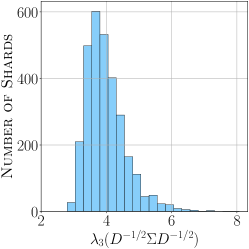
(a) DeepImage

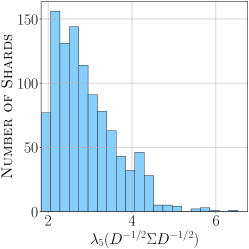
(b) GloVe

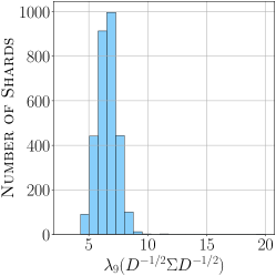
(c) MsMarco-MiniLM

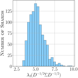
(d) Music

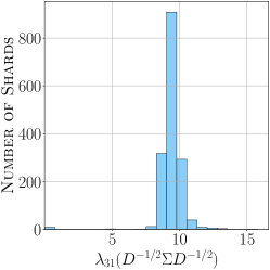
(e) Nq-Ada2

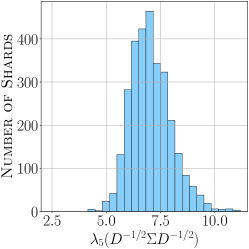
(f) Text2Image

Figure 5: Histogram of the $(t+1)$-th eigenvalue for each dataset. For each dataset, we pick the partitioning and $t$ which we use in the plots from Figure 6. Plots show that almost all shards for all datasets have $(t+1)$-th eigenvalue bounded away from $2$, except for some shards for GloVe and one for Nq-Ada2.

Second assumption.

Since $\Sigma=\frac{1}{n}\sum_{i=1}^{n}(x_{i}-\mu)(x_{i}-\mu)^{\top}$ for the $n$ points $x_{1},\dots,x_{n}\in\operatorname*{\mathbb{R}}^{d}$ and mean $\mu=\sum_{i=1}^{n}x_{i}/n$ in the shard, it is in fact positive semi-definite. In particular the entries of the diagonal are non-negative. While in the worst case, the diagonal can have arbitrarily large entries compared to its smallest entries, in practice this is rarely the case. While we do not explore how to remove this assumption, there are several mechanisms to do so in practice such as applying a random rotations or pseudo-random rotations Ailon and Chazelle [2009], Woodruff [2014], Ailon and Liberty [2013] to the datapoints $x_{1},\dots,x_{n}$ in each shard before using Algorithm 1. It is well known (e.g. Lemma 1 in Ailon and Chazelle [2009]) that after applying such transforms that the coordinates of the vectors are “roughly equal,” thereby ensuring that the diagonal of the covariance has entries of comparable magnitude. We leave the exploration of removing this assumption to future work.

Appendix D Additional experimental results

This section presents our full experimental results for completeness.

D.1 Clustering by Spherical KMeans

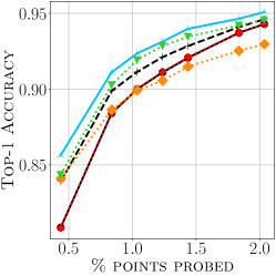
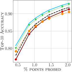
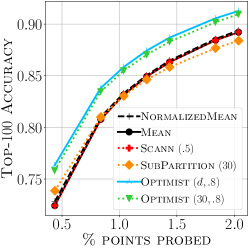
(a) Nq-Ada2

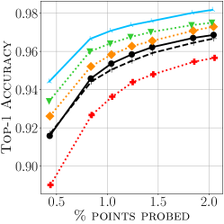
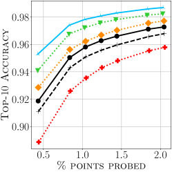
(b) Music

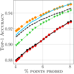
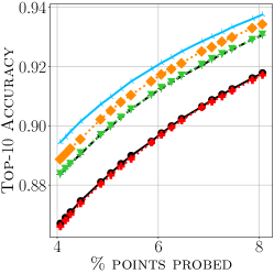
(c) GloVe

Figure 6: Top-$k$ recall versus the number of probed data points. Datasets are partitioned with Spherical KMeans. Scann has parameter $T$, SubPartition $t$ (leading to $t+2$ sub-partitions per shard), and Optimist rank $t$ and degree of optimism $\delta$.

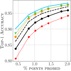
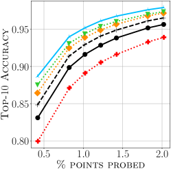
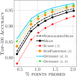
(d) Text2Image

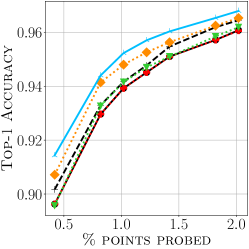
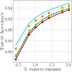
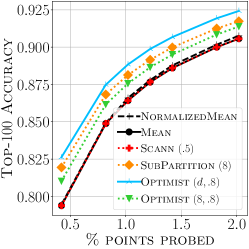
(e) MsMarco-MiniLM

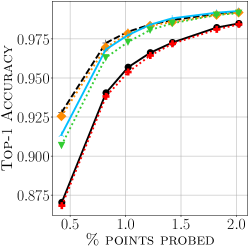
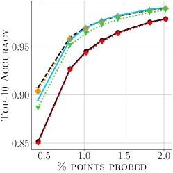
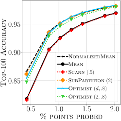
(f) DeepImage

Figure 6: Top-$k$ recall versus the number of probed data points. Datasets are partitioned with Spherical KMeans. Scann has parameter $T$, SubPartition $t$ (leading to $t+2$ sub-partitions per shard), and Optimist rank $t$ and degree of optimism $\delta$.

D.2 Clustering by Standard KMeans

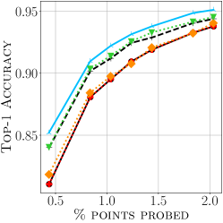
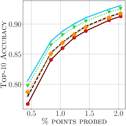
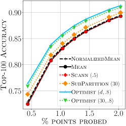
(a) Nq-Ada2

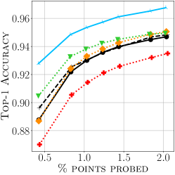
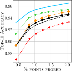
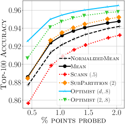
(b) Music

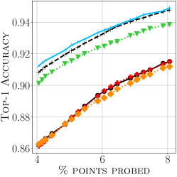
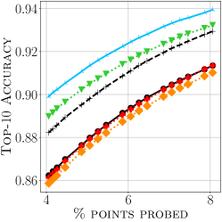
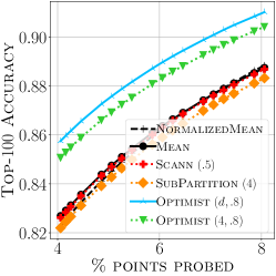
(c) GloVe

Figure 7: Top-$k$ recall versus the number of probed data points. Datasets are partitioned with Standard KMeans. Scann has parameter $T$, SubPartition $t$ (leading to $t+2$ sub-partitions per shard), and Optimist rank $t$ and degree of optimism $\delta$.

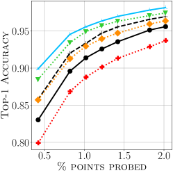
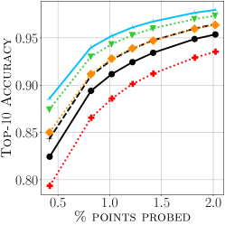
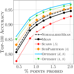
(d) Text2Image

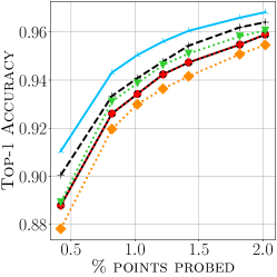
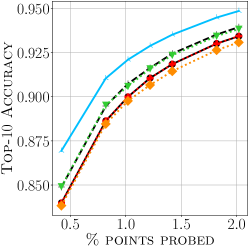
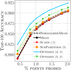
(e) MsMarco-MiniLM

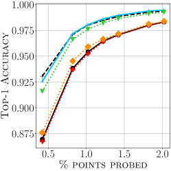
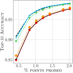
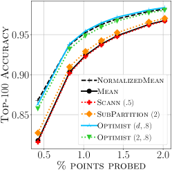
(f) DeepImage

Figure 7: Top-$k$ recall versus the number of probed data points. Datasets are partitioned with Standard KMeans. Scann has parameter $T$, SubPartition $t$ (leading to $t+2$ sub-partitions per shard), and Optimist rank $t$ and degree of optimism $\delta$.

D.3 Clustering by GMM

We note that, due to the dimensionality of the Nq-Ada2 dataset, we were unable to complete GMM clustering on this particular dataset.

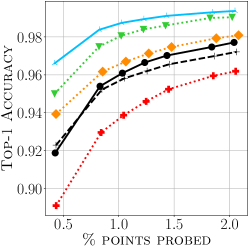
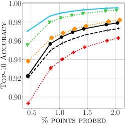
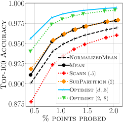
(a) Music

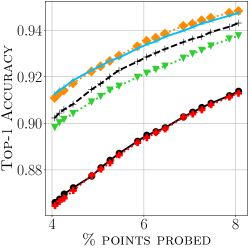
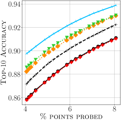
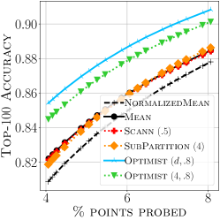
(b) GloVe

Figure 8: Top-$k$ recall versus the number of probed data points. Datasets are partitioned with Gaussian Mixture Model. Scann has parameter $T$, SubPartition $t$ (leading to $t+2$ sub-partitions per shard), and Optimist rank $t$ and degree of optimism $\delta$.

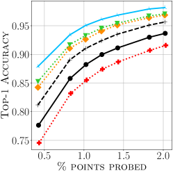
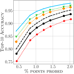
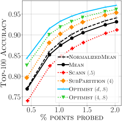
(c) Text2Image

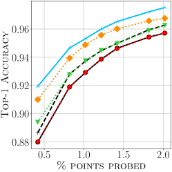
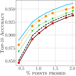
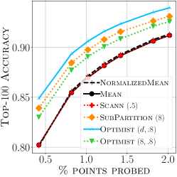
(d) MsMarco-MiniLM

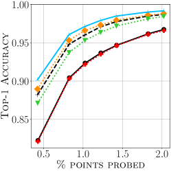
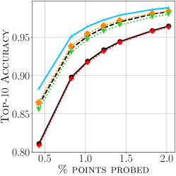
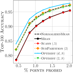
(e) DeepImage

Figure 8: Top-$k$ recall versus the number of probed data points. Datasets are partitioned with Gaussian Mixture Model. Scann has parameter $T$, SubPartition $t$ (leading to $t+2$ sub-partitions per shard), and Optimist rank $t$ and degree of optimism $\delta$.

Appendix E Effect of parameters

Recall that the final Optimist algorithm takes two configurable parameters: $t$, the rank of the covariance sketch in Equation (7); and $\delta$, the degree of optimism in Problem 1. In this section, we examine the effect of these parameters on the performance of Optimist.

Figure 9 visualizes the role played by $t$. It comes as no surprise that larger values of $t$ lead to a better approximation of the covariance matrix. What we found interesting, however, is the remarkable effectiveness of a sketch that simply retains the diagonal of the covariance, denoted by $\textsc{Optimist}(0,\cdot)$, in the settings of $k$ we experimented with (i.e., $k\in\{1,10,100\}$).

In the same figure, we have also included two configurations of SubPartition: one with just $2$ sub-partitions, denoted by $\textsc{SubPartition}(0)$, and another with $t+2$ sub-partitions, $\textsc{SubPartition}(t)$. These help put the performance of Optimist with various ranks in perspective. In particular, we give the SubPartition baseline the same amount of information and contrast its recall with Optimist.

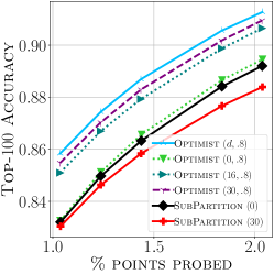
(a) Nq-Ada2

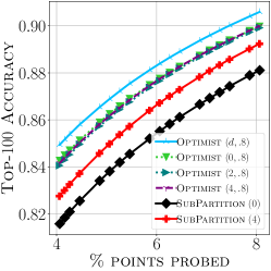
(b) GloVe

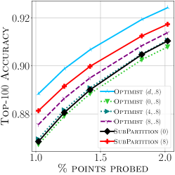
(c) MsMarco-MiniLM

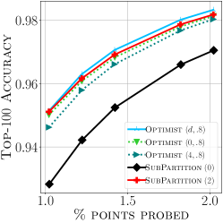
(d) DeepImage

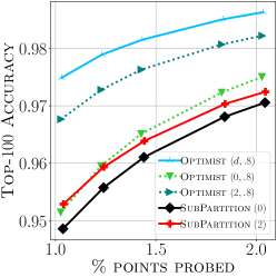
(e) Music

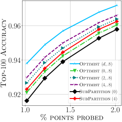
(f) Text2Image

Figure 9: Top-$100$ recall versus the number of probed data points. Datasets are partitioned with Spherical KMeans. We compare a range of values for the rank of the covariance sketch ($t$) with SubPartition with the same capacity as Optimist with the smallest and largest ranks. $\textsc{Optimist}(0,\cdot)$ denotes a sketch that only retains the diagonal of the covariance matrix; and $\textsc{SubPartition}(t)$ means every shard is partitioned into $t+2$ sub-partitions.

We turn to Figure 10 to understand the impact of $\delta$. It is clear that encouraging Optimist to be too optimistic can lead to sub-optimal performance. That is because of our reliance on the Chebyshev’s inequality, which can prove too loose, leading to an overestimation of the maximum value. Interestingly, $\delta\in(0.6,0.8)$ appears to yield better recall across datasets.

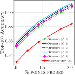
(a) Nq-Ada2

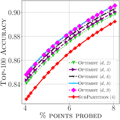
(b) GloVe

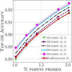
(c) MsMarco-MiniLM

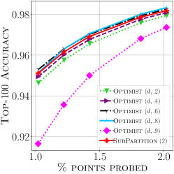
(d) DeepImage

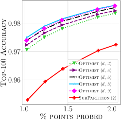
(e) Music

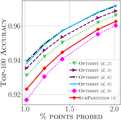
(f) Text2Image

Figure 10: Top-$100$ recall versus the number of probed data points. Datasets are partitioned with Spherical KMeans. We compare a range of values for the optimism parameter ($\delta$) with the strongest baseline (SubPartition) from Appendix D.1. As $\delta\rightarrow 1$, Optimist becomes more optimistic.

Appendix F Prediction error

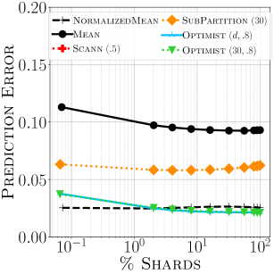
(a) Nq-Ada2

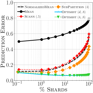
(b) GloVe

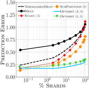
(c) MsMarco-MiniLM

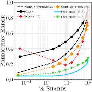
(d) DeepImage

(e) Music

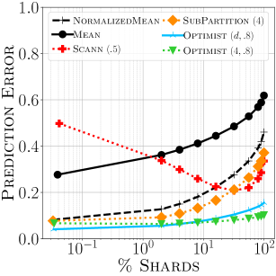
(f) Text2Image

Figure 11: Mean prediction error $\mathcal{E}_{\ell}(\tau,\cdot)$, defined in Equation (8), versus $\ell$ (expressed as percent of total number of shards), for various routers and datasets.

References

- Ailon and Chazelle [2009] Nir Ailon and Bernard Chazelle. The fast johnson–lindenstrauss transform and approximate nearest neighbors. SIAM Journal on computing, 39(1):302–322, 2009.
- Ailon and Liberty [2013] Nir Ailon and Edo Liberty. An almost optimal unrestricted fast johnson-lindenstrauss transform. ACM Transactions on Algorithms (TALG), 9(3):1–12, 2013.
- Andre et al. [2021] Fabien Andre, Anne-Marie Kermarrec, and Nicolas Le Scouarnec. Quicker adc: Unlocking the hidden potential of product quantization with simd. IEEE Transactions on Pattern Analysis and Machine Intelligence, 43(5):1666–1677, 5 2021.
- Auvolat et al. [2015] Alex Auvolat, Sarath Chandar, Pascal Vincent, Hugo Larochelle, and Yoshua Bengio. Clustering is efficient for approximate maximum inner product search, 2015.
- Babenko and Lempitsky [2012] Artem Babenko and Victor Lempitsky. The inverted multi-index. In 2012 IEEE Conference on Computer Vision and Pattern Recognition, pages 3069–3076, 2012.
- Bentley [1975] Jon Louis Bentley. Multidimensional binary search trees used for associative searching. Communications of the ACM, 18(9):509–517, 9 1975.
- Braverman et al. [2022] Vladimir Braverman, Aditya Krishnan, and Christopher Musco. Sublinear time spectral density estimation. In Proceedings of the 54th Annual ACM SIGACT Symposium on Theory of Computing, pages 1144–1157, 2022.
- Bruch [2024] Sebastian Bruch. Foundations of Vector Retrieval. Springer Nature Switzerland, 2024.
- Bruch et al. [2024] Sebastian Bruch, Franco Maria Nardini, Amir Ingber, and Edo Liberty. Bridging dense and sparse maximum inner product search. ACM Transactions on Information Systems, 2024. (to appear).
- Chierichetti et al. [2007] Flavio Chierichetti, Alessandro Panconesi, Prabhakar Raghavan, Mauro Sozio, Alessandro Tiberi, and Eli Upfal. Finding near neighbors through cluster pruning. In Proceedings of the 26th ACM SIGMOD-SIGACT-SIGART Symposium on Principles of Database Systems, pages 103–112, 2007.
- Dasgupta and Sinha [2015] Sanjoy Dasgupta and Kaushik Sinha. Randomized partition trees for nearest neighbor search. Algorithmica, 72(1):237–263, 5 2015.
- Dhillon and Modha [2001] Inderjit S. Dhillon and Dharmendra S. Modha. Concept decompositions for large sparse text data using clustering. Machine Learning, 42(1):143–175, January 2001.
- Douze et al. [2024] Matthijs Douze, Alexandr Guzhva, Chengqi Deng, Jeff Johnson, Gergely Szilvasy, Pierre-Emmanuel Mazaré, Maria Lomeli, Lucas Hosseini, and Hervé Jégou. The faiss library, 2024.
- Ge et al. [2014] Tiezheng Ge, Kaiming He, Qifa Ke, and Jian Sun. Optimized product quantization. IEEE Transactions on Pattern Analysis and Machine Intelligence, 36(4):744–755, 2014.
- Guo et al. [2020] Ruiqi Guo, Philip Sun, Erik Lindgren, Quan Geng, David Simcha, Felix Chern, and Sanjiv Kumar. Accelerating large-scale inference with anisotropic vector quantization. In Proceedings of the 37th International Conference on Machine Learning, 2020.
- Indyk and Motwani [1998] Piotr Indyk and Rajeev Motwani. Approximate nearest neighbors: Towards removing the curse of dimensionality. In Proceedings of the 30th Annual ACM Symposium on Theory of Computing, pages 604–613, 1998.
- Jaiswal et al. [2022] Shikhar Jaiswal, Ravishankar Krishnaswamy, Ankit Garg, Harsha Vardhan Simhadri, and Sheshansh Agrawal. Ood-diskann: Efficient and scalable graph anns for out-of-distribution queries, 2022.
- Jayaram Subramanya et al. [2019] Suhas Jayaram Subramanya, Fnu Devvrit, Harsha Vardhan Simhadri, Ravishankar Krishnawamy, and Rohan Kadekodi. Diskann: Fast accurate billion-point nearest neighbor search on a single node. In Advances in Neural Information Processing Systems, volume 32, 2019.
- Jégou et al. [2011] Herve Jégou, Matthijs Douze, and Cordelia Schmid. Product quantization for nearest neighbor search. IEEE Transactions on Pattern Analysis and Machine Intelligence, 33(1):117–128, 2011.
- Johnson et al. [2021] Jeff Johnson, Matthijs Douze, and Hervé Jégou. Billion-scale similarity search with gpus. IEEE Transactions on Big Data, 7(3):535–547, 2021.
- Kalantidis and Avrithis [2014] Yannis Kalantidis and Yannis Avrithis. Locally optimized product quantization for approximate nearest neighbor search. In 2014 IEEE Conference on Computer Vision and Pattern Recognition, pages 2329–2336, 2014.
- Kong and Valiant [2017] Weihao Kong and Gregory Valiant. Spectrum estimation from samples. The Annals of Statistics, 45(5):2218–2247, 2017.
- Kwiatkowski et al. [2019] Tom Kwiatkowski, Jennimaria Palomaki, Olivia Redfield, Michael Collins, Ankur Parikh, Chris Alberti, Danielle Epstein, Illia Polosukhin, Jacob Devlin, Kenton Lee, Kristina Toutanova, Llion Jones, Matthew Kelcey, Ming-Wei Chang, Andrew M. Dai, Jakob Uszkoreit, Quoc Le, and Slav Petrov. Natural questions: A benchmark for question answering research. Transactions of the Association for Computational Linguistics, 7:452–466, 2019.
- Lattimore and Szepesvári [2020] Tor Lattimore and Csaba Szepesvári. Bandit algorithms. Cambridge University Press, 2020.
- Malkov and Yashunin [2020] Yu A. Malkov and D. A. Yashunin. Efficient and robust approximate nearest neighbor search using hierarchical navigable small world graphs. IEEE Transactions on Pattern Analysis and Machine Intelligence, 42(4):824–836, 4 2020.
- Morozov and Babenko [2018] Stanislav Morozov and Artem Babenko. Non-metric similarity graphs for maximum inner product search. In Advances in Neural Information Processing Systems, volume 31. Curran Associates, Inc., 2018.
- Nguyen et al. [2016] Tri Nguyen, Mir Rosenberg, Xia Song, Jianfeng Gao, Saurabh Tiwary, Rangan Majumder, and Li Deng. Ms marco: A human generated machine reading comprehension dataset, November 2016.
- Norouzi and Fleet [2013] Mohammad Norouzi and David J. Fleet. Cartesian k-means. In Proceedings of the 2013 IEEE Conference on Computer Vision and Pattern Recognition, pages 3017–3024, 2013.
- Pearson [1936] Karl Pearson. Method of moments and method of maximum likelihood. Biometrika, 28(1/2):34–59, 1936.
- Pennington et al. [2014] Jeffrey Pennington, Richard Socher, and Christopher Manning. GloVe: Global vectors for word representation. In Proceedings of the 2014 Conference on Empirical Methods in Natural Language Processing, pages 1532–1543, Doha, Qatar, October 2014.
- Simhadri et al. [2022] Harsha Vardhan Simhadri, George Williams, Martin Aumüller, Matthijs Douze, Artem Babenko, Dmitry Baranchuk, Qi Chen, Lucas Hosseini, Ravishankar Krishnaswamny, Gopal Srinivasa, Suhas Jayaram Subramanya, and Jingdong Wang. Results of the neurips’21 challenge on billion-scale approximate nearest neighbor search. In Proceedings of the NeurIPS 2021 Competitions and Demonstrations Track, volume 176 of Proceedings of Machine Learning Research, pages 177–189, Dec 2022.
- Singh et al. [2021] Aditi Singh, Suhas Jayaram Subramanya, Ravishankar Krishnaswamy, and Harsha Vardhan Simhadri. Freshdiskann: A fast and accurate graph-based ann index for streaming similarity search, 2021.
- Vecchiato et al. [2024] Thomas Vecchiato, Claudio Lucchese, Franco Maria Nardini, and Sebastian Bruch. A learning-to-rank formulation of clustering-based approximate nearest neighbor search. In Proceedings of the 47th International ACM SIGIR Conference on Research and Development in Information Retrieval, 2024. (to appear).
- Woodruff [2014] David P. Woodruff. Sketching as a tool for numerical linear algebra. Foundations and Trends in Theoretical Computer Science, 10(1–2):1–157, Oct 2014. ISSN 1551-305X.
- Wu et al. [2017] Xiang Wu, Ruiqi Guo, Ananda Theertha Suresh, Sanjiv Kumar, Daniel N Holtmann-Rice, David Simcha, and Felix Yu. Multiscale quantization for fast similarity search. In Advances in Neural Information Processing Systems, volume 30, 2017.
- Yandex and Lempitsky [2016] Artem Babenko Yandex and Victor Lempitsky. Efficient indexing of billion-scale datasets of deep descriptors. In 2016 IEEE Conference on Computer Vision and Pattern Recognition, pages 2055–2063, 2016.