Modeling citation worthiness by using attention-based Bidirectional Long Short-Term Memory networks and interpretable models

Abstract

Scientist learn early on how to cite scientific sources to support their claims. Sometimes, however, scientists have challenges determining where a citation should be situated—or, even worse, fail to cite a source altogether. Automatically detecting sentences that need a citation (i.e., citation worthiness) could solve both of these issues, leading to more robust and well-constructed scientific arguments. Previous researchers have applied machine learning to this task but have used small datasets and models that do not take advantage of recent algorithmic developments such as attention mechanisms in deep learning. We hypothesize that we can develop significantly accurate deep learning architectures that learn from large supervised datasets constructed from open access publications. In this work, we propose a Bidirectional Long Short-Term Memory (BiLSTM) network with attention mechanism and contextual information to detect sentences that need citations. We also produce a new, large dataset (PMOA-CITE) based on PubMed Open Access Subset, which is orders of magnitude larger than previous datasets. Our experiments show that our architecture achieves state of the art performance on the standard ACL-ARC dataset ($F_{1}=0.507$) and exhibits high performance ($F_{1}=0.856$) on the new PMOA-CITE. Moreover, we show that it can transfer learning across these datasets. We further use interpretable models to illuminate how specific language is used to promote and inhibit citations. We discover that sections and surrounding sentences are crucial for our improved predictions. We further examined purported mispredictions of the model, and uncovered systematic human mistakes in citation behavior and source data. This opens the door for our model to check documents during pre-submission and pre-archival procedures. We discuss limitations of our work and make this new dataset, the code, and a web-based tool available to the community.

1 Introduction

Scientists and journalists have challenges determining proper citations in the ever increasing sea of information. More fundamentally, when and where a citation is needed—sometimes called citation worthiness—is a crucial first step to solve this challenge. In the general media, some problematic stories have shown that claims need citations to make them verifiable—e.g., the debunked A Rape on Campus article in the Rolling Stone magazine (wiki:2018). Analyses of Wikipedia have revealed that lack of citations correlates with an article’s immaturity (jack2014citation; chen2012citation). In science, the lack of citations leaves readers wondering how results were built upon previous work (aksnes2009researchers). Also, it precludes researchers from getting appropriate credit, important during hiring and promotion (gazni2016author). The sentences surrounding a citation provide rich information for common semantic analyses, such as information retrieval (nakov2004citances). There should be methods and tools to help scientists cite; in this work, we want to understand where citations should be situated in a paper with the goal of automatically suggesting them.

We first review a closely related problem: citation recommendation. Several research groups have studied how to recommend citations at the article and local levels, separately. At the article level, kuccuktuncc2012direction uses graph based methods for estimating citation relationships between papers. mcnee2002recommending and torres2004enhancing use collaborative filtering to make such suggestions by bootstrapping on collective citation patterns. These techniques work well for making article-level citation recommendations and they frequently rely on knowing where a citation should be located. At the local level, HeContextawareCitationRecommendation2010 propose context aware citation recommendation by using local contextual information of the places where citations are made. More recently, other groups have used more sophisticated neural network models to estimate a semantic representation of sentences—e.g., HuangNeuralProbabilisticModela use distributed representations, ebesu2017neural use auto-encoders, and BhagavatulaContentBasedCitationRecommendation2018 use a two-step process to first embed documents into a vector representation and then rank them according to a relevance estimation task. These techniques have shown that it is possible to provide detailed sentence level suggestions if the place to put a citation is already known. This implies that detecting which sentences need a citation is a crucial first step for sentence-level citation recommendation.

Relatively much less work has been done on detecting where a citation should be. he2011citation were the first to introduce the task of identifying candidate location where citations are needed in the context of scientific articles. jack2014citation studied how to detect citation needs in Wikipedia. peng2016news used the learning-to-rank framework to solve citation recommendation in news articles. These are very diverse domains, and therefore it is difficult to generalize results. We contend that a large standard dataset of citation location with open code and services would significantly improve the systematic study of the problem. Thus, the task of citation worthiness detection is relatively new and needs further exploration.

Recently, Recurrent Neural Networks (RNN) and Convolutional Neural Networks (CNN) architectures have been used for the detection of citation worthiness. The group of bonabCitationWorthinessSentences2018 applied CNN based classifiers, achieving state of art performance. farber2018cite proposed stacking a RNN on top of a CNN, achieving good performance as well. However, one of the problems with RNN networks is that they tend to dismiss long-distance dependencies. The attention mechanism has been shown to fix some of this issue, and it can potentially help for the detection of citation worthiness.

The attention mechanism is a relatively recent development in neural networks motivated by human visual attention. Humans get more information from the region they pay attention to, and perceive less from other regions. An attention mechanism in neural networks was first introduced in computer vision (sunObjectbasedVisualAttention2003), and later applied to NLP for machine translation (bahdanauNeuralMachineTranslation2014). Attention has quickly become adopted in other sub-domains. luongEffectiveApproachesAttentionbased2015 examined several attention scoring functions for machine translation. liDatasetNeuralRecurrent2016 used attention mechanisms to improve results in a question-answering task. zhouAttentionBasedBidirectionalLong2016 made use of an attention-based LSTM network to do relational classification. linStructuredSelfattentiveSentence2017 used attention to improve sentence embedding. Recently, vaswaniAttentionAllYou2017a built an architecture called transformer that promises to replace recurrent neural networks (RNNs) altogether by only using attention mechanisms. These results show the advantage of attention for NLP tasks and thus its potential benefit for citation worthiness.

In this study, we formulate the detection of sentences that need citations as a classification task that can be effectively solved with a deep learning architecture that relies on an attention mechanism. Our contributions are the following:

A deep learning architecture based on bidirectional LSTM with attention and contextual information for citation worthiness

A new large scale dataset for the citation worthiness task that is 300 times bigger that the next current alternative

A set of classic interpretable models that provide insights into the language used for making citations

An examination of common citation mistakes—from unintentional omissions to potentially problematic mis-citations

An evaluation of transfer learning between our proposed dataset and the ACL-ARC dataset

The code to produce the dataset and results, a web-based tool for the community to evaluate our predictions, and the pre-processed dataset.

2 Materials and methods

2.1 Problem Formulation

We consider a paper as a sequence of sentences, and sentences as a sequence of words. We denote a paper as $D$, a word as $w$, and a sentence as $S$, $S$$=[w_{1},w_{2},...,w_{N}]$. The citation location is the location where the paper cites a reference within the sequence of words—e.g., "[6,8]". The citing sentence is a sentence that contains one or more citations, and we denote it as $S^{c}$. A non-citing sentence is denoted as $S^{nc}$. Finally, citation context could be any information describing the context of a sentence. These definitions will be used throughout this article.

There are multiple ways of defining a citation context. A frequently employed approach is to define the citation context as a sequence of words around citation locations (HuangNeuralProbabilisticModela; mikolov2013distributed; duma2016applying). The length of such sequence may vary from paper to paper—HeContextawareCitationRecommendation2010 specified the context as a fixed window of 100 words; duma2014citation experimented with 5, 10, 20 and 30 words. However, the number of words associated with a citation may differ on a case-by-case basis (ritchie2009citation), and arbitrarily truncating a sentence due to the size of a window could reduce the strength of contextual signal. As others have observed (i.e., allerton1969sentence; frajzyngier2005linguistic; halliday2014introduction), humans use a sentence as the fundamental unit to express thoughts. Therefore, we will use sentences as the minimum unit for our algorithm. While some researchers only consider the citing sentence as the context (he2012position), we also consider the previous and next sentences as citation context. Furthermore, we observe that the section $Sec$ (e.g. introduction, methods, results, discussion, and so forth) may affect whether a sentence needs a citation. Therefore, we include section as part of the context. The context, then, is denoted by $CC=\{S_{n-1},S_{n}^{c},S_{n+1},Sec\}$.

We now state the citation worthiness problem. The user submits a manuscript without reference list and without citation placeholders. Our goal is to predict for each sentence whether it needs a citation (Fig. 1). Since there are only two outputs, we cast this prediction as a binary classification task.

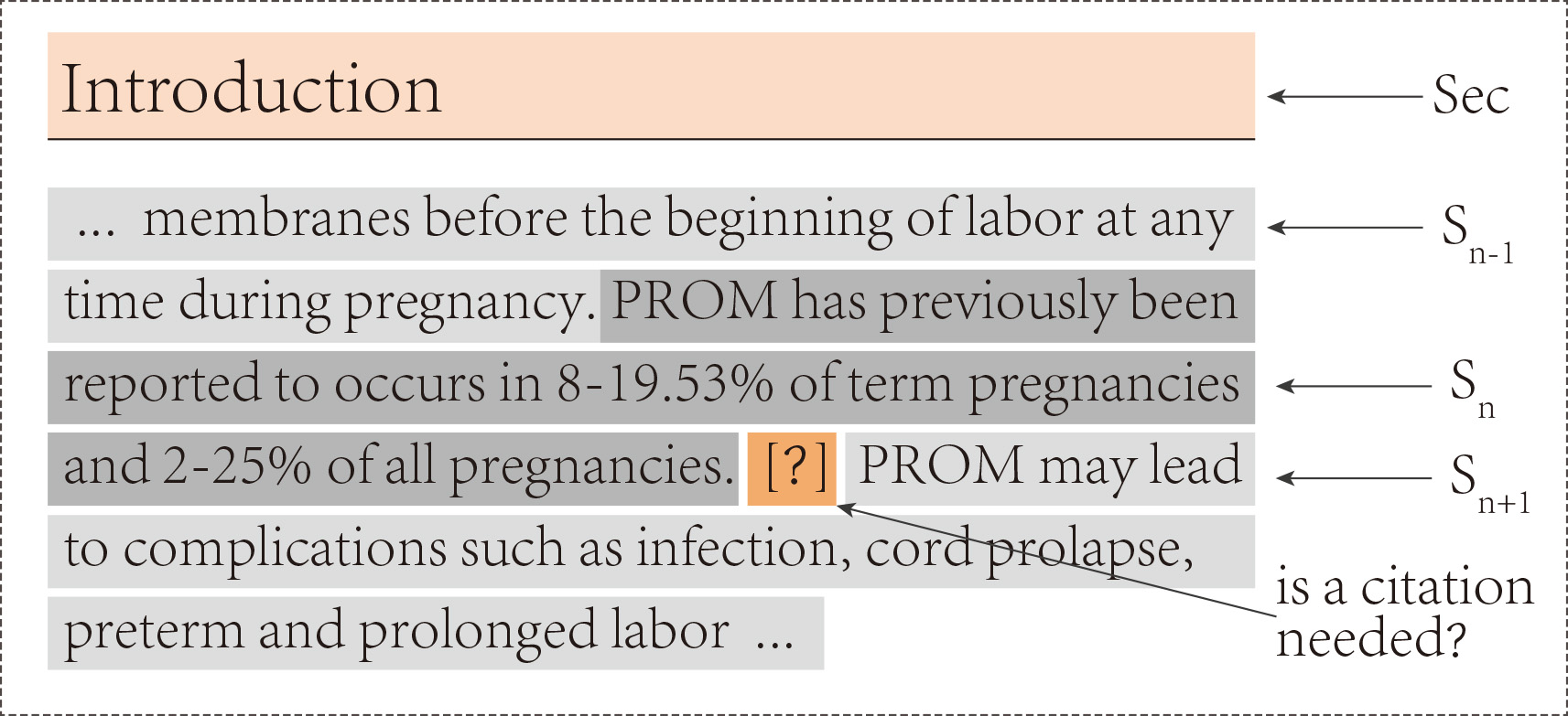
Figure 1: Citation worthiness prediction problem. For a given sentence ($S_{n}$), the goal of the task is to predict whether it needs a citation. The prediction task may use the section, the previous and next sentences (i.e., $S_{n-1}$ and $S_{n+1}$) for such prediction.

2.2 Data sources and data pre-processing

2.2.1 ACL Anthology Reference Corpus

The ACL Anthology Reference Corpus (ACL-ARC) is a collection of scientific articles in Computational Linguistics. The ACL-ARC 1.0 dataset consists of 10,921 articles up to February 2007, including the source PDF, automatically extracted full text, and the metadata for the articles. In order to use the ACL-ARC dataset, we need to remove some noisy sentences, such as footnotes, mathematical equations, and URLs. bonabCitationWorthinessSentences2018 carried out all these pre-processing steps and made the data available on the Internet. This dataset consists of 85,778 sentences with citations and 1,142,275 sentences without citations. More statistics are presented in Table 2.

2.2.2 PubMed Central Open Access Subset

PubMed Central Open Access subset (PMOAS) is a full-text collection of scientific literature in bio-medical and life sciences. PMOAS is created by the US’s National Institutes of Health. We obtain a snapshot of PMOAS on August, 2019. The dataset consists of more than 2 million full-text journal articles organized in well-structured XML files (Fig. 2). The XML format follow the Journal Article Tag Suite (JATS) which developed by the National Information Standards Organization (JATS2013).

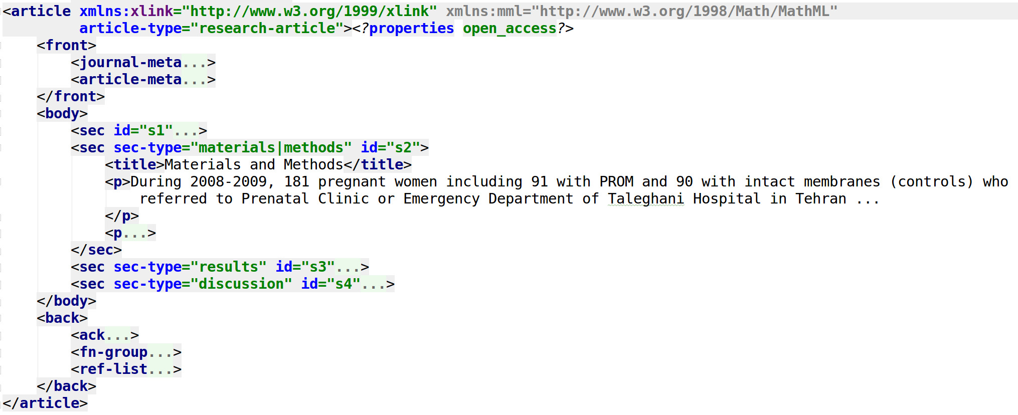
Figure 2: A sample of a PMC Open Access Subset (PMOAS) XML. The structure is defined by a standard Document Type Definition (DTD) which makes all articles consistent. In particular, the tag and attributes of a citation are well known.

We now describe how we prepare the dataset.

Sentence segmentation and outlier removal. Text in a PMOAS XML file is marked by a paragraph tag, but there might be other XML tags inside paragraph tags. Therefore, we needed to get all the text of a paragraph from XML tags recursively and break paragraphs into sentences. We used spaCy Python package to do the sentence splitting (spacy2). However, there are some outliers in the sentences (e.g. long gene sequences with more then 10 thousand characters that are treated as one sentence). Base on the distribution of sentence length (see Figure 3), we remove the sentences that are outliers either in character or word length. We winsorize 5% and 95% quantiles. For character-wise length, this amounts to 19 characters for 5% quantile and 275 characters for 95% quantile. For word-wise length, it is 3 words and 42 words, respectively.

Hierarchical tree-like structure. By using section and paragraph tagging information in the XML file and the sentences we extracted in previous step, we construct a hierarchical tree-like structure of the articles. In this structure, sentences are contained within paragraphs, which in turn are contained within sections. For each section, we extract the section-type attribute from the XML file which indicates which kind of section is (from a pre-defined set). For those sections without a section-type, we use the section title instead.

Citation hints removal. The citing sentence usually has some explicit hints which discloses a citation. This provides too much information for the model training and it does not faithfully represents a real-world application scenario. Thus, we removed all the citation hints by regular expression (see Table 1).

Noise removal. There are other filters applied to remove noise from sentences. We apply the following cleanup steps: trim white spaces at beginning and end of a sentence, remove the numbers or punctuations at the beginning of a sentence, and remove numbers at the end of a sentence.

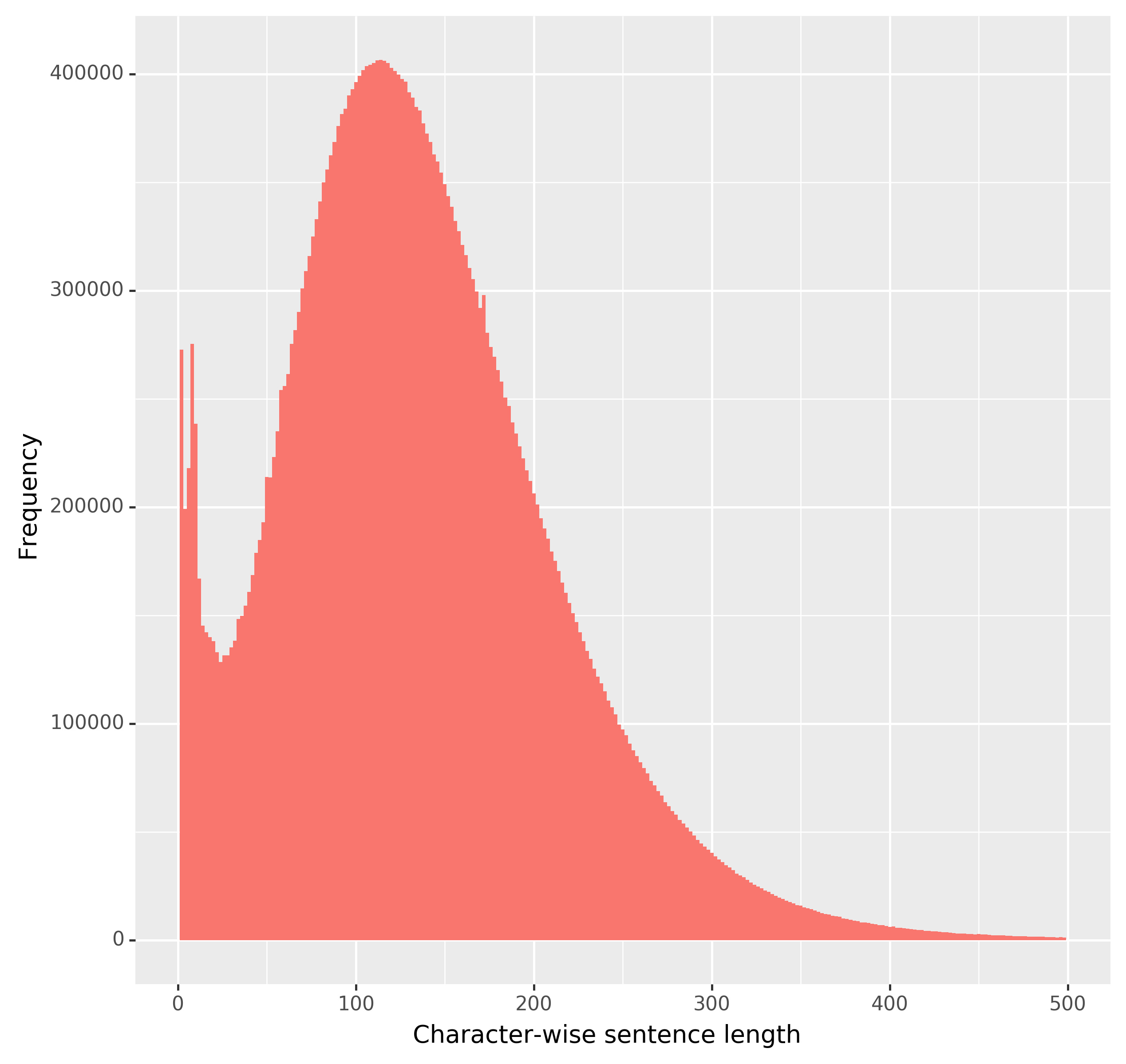
(a) Character count distribution of sentences

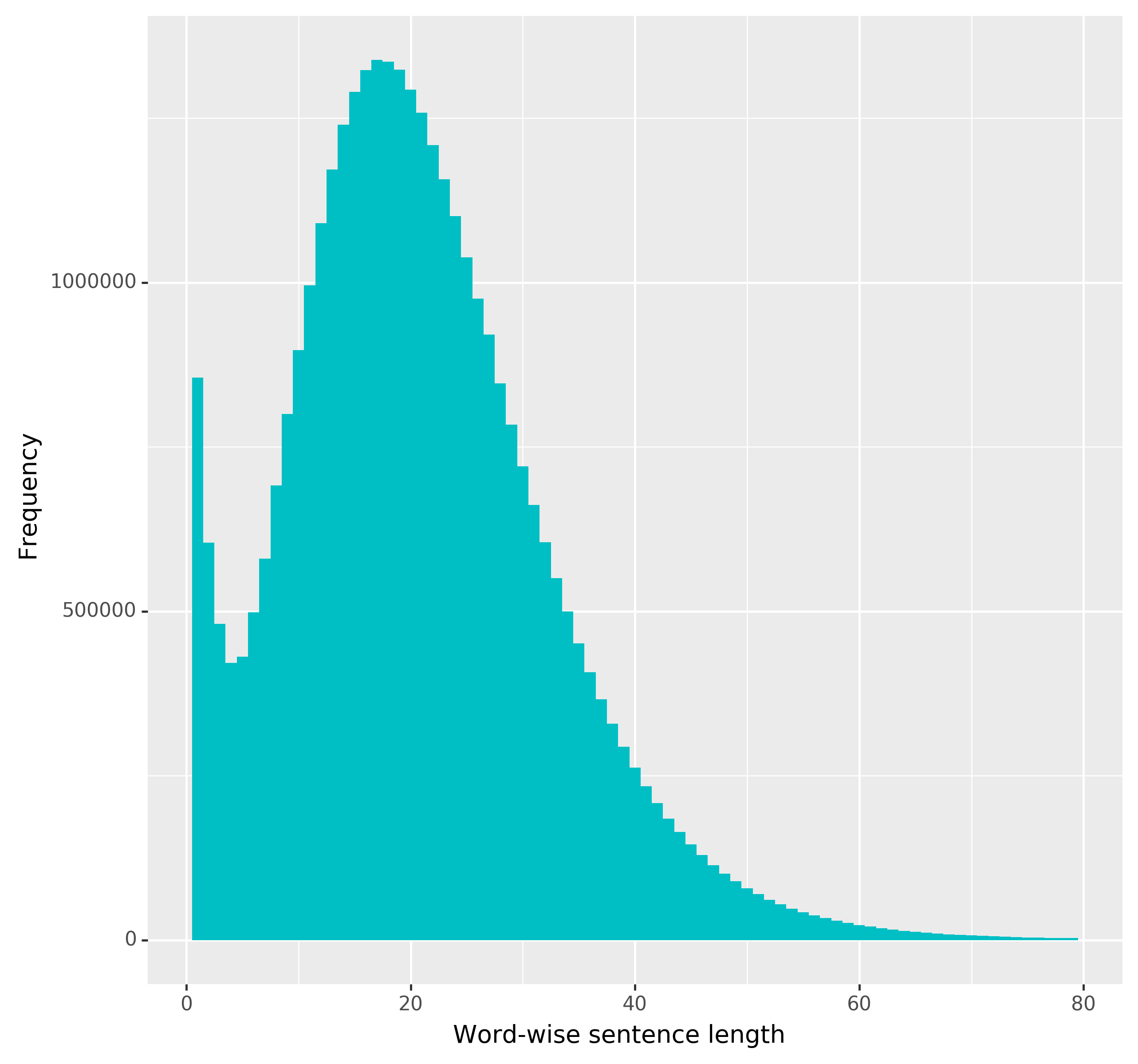
(b) Word count distribution of sentences

Figure 3: The distribution of sentence length

Table 1: regular expression to remove the citation hints

Regular expression	Description	Example
(?<!^)([\[\(])[\s]* ([\d][\s\,\-\–\;\-]*)* [\d][\s]*[\]\)]	numbers contained in parentheses and square brackets	“[1, 2]”, “[ 1- 2]”, “(1-3)”, “(1,2,3)”, “[1-3, 5]”, “[8],[9],[12]”, “( 1-2; 4-6; 8 )”
[\(\[]\s*([^\(\)\[\]]* (((16|17|18|19|20) \d{2}(?!\d))| (et[\. \s\\xa0]*al\.)) [^\(\)]*)?[\)\]]	text within parentheses	“(Kim and li, 2008)”, “(Heijman , 2013b)”, “(Tárraga , 2006; Capella-Gutiérrez , 2009)”, “(Kobayashi et al., 2005)”, “(Richart and Barron, 1969; Campion et al, 1986)”, “(Nasiell et al, 1983, 1986)”
et[\. \s\\xa0]+al[\.\s\(\[]* ((16|17|18|19|20)\d {2})*[)\] \s]*(?=\D)	remove et al. and the following years	“et al.”, “et al. 2008”, “et al. (2008)”

After the processing, we get a dataset with approximately 309 million sentences. However, due to the computational cost and in order to make all of our analysis manageable, we randomly sample articles whose sentences produce close to one million sentences. We further split the one million sentences, 60% for training, 20% for validating, and 20% for testing. We present some characteristics of the whole dataset and one million sentence sample in Table 2.

Table 2: Characteristics of the ACL-ARC dataset, whole PMOA-CITE dataset and a sample of PMOA-CITE which contains one million sentences

Items	ACL-ARC	PMOA-CITE	PMOA-CITE sample
articles	N/A	2,075,208	6,754
sections	N/A	9,903,173	32,198
paragraphs	N/A	62,351,079	202,047
sentences	1,228,052	309,407,532	1,008,042
sentences without citations	1142275	249,138,591	811,659
sentences with citations	85777	60,268,941	196,383
average characters per sentence	131	132	132
average words per sentence	22	20	20

2.3 Text Representation

Some of our models use different text representations predicting citation worthiness. We now describe them.

Bag of words (BoW) representation This is a widely-used representation where the order of words in the original text is ignored and only word frequencies are maintained. While this representation is clearly very simple (see harris1954distributional), it has shown remarkable performance in several tasks.

We follow the standard definition of term-frequency inverse term-frequency (tf-idf) to construct our bag of words (BoW) representation (manning2008introduction). Our BoW representation for a sentence $S$ which consists of $n$ words will therefore be the vector of all tf-idf values in document $D_{i}$.

$$\text{BoW}(S)=[\text{tf-idf}_{w_{1},D_{i}},...,\text{tf-idf}_{w_{n},D_{i}\cdot}]$$ (1)

Sometimes, it is not possible to capture some language subtleties using singular words as tokens. For example, “play football” has a different meaning than “football play”. Therefore, it is common to also keep track of combinations of words in what are known as $n$-gram language models (jurafsky2014speech). In our analysis, we use unigrams and bigrams to construct the bag-of-words representation.

Topic modeling based (TM) representation Topic modeling is a machine learning technique whose goal is to represent a document as a mixture of a small number of “topics”. This reduces the dimensionality needed to represent a document compared to bag-of-words. There are several topic models available including Latent Semantic Analysis (LSA) and Non-negative Matrix Factorization (NMF). In this paper, we use Latent Dirichlet Allocation (LDA), which is one of the most popular and well-motivated approaches (for discussions of its advantage, see blei2003latent; blei2012probabilistic; however, also see some shortcomings in lancichinetti2015high).

Distributed word representation While topic models can extract statistical structure across documents, they do a relatively poor job at extracting information within documents. In particular, topic models are not meant to find contextual relationships between words. Word embedding methods, in contrast, are based on the distributional hypothesis which states that words that occur in the same context are likely to have similar meaning (harris1954distributional). The famous statement “you shall know a word by the company it keeps” by firth1957synopsis is a concise guideline for word embedding: a word could be represented by means of the words surrounding it. In word embedding, words are represented as fixed-length vectors that attempt to approximate their semantic meaning within a document.

There are several distributed word representation methods but one of the most successful and well-known is GloVe by pennington2014glove. We use GloVe word vectors with 300 dimensions, pre-trained on 6 billion tokens.

2.4 Sentence features and contextual features

After sentence processing, we can get features from the sentence itself and its context. For sentence, we get text representation, the character-wise sentence length, the word-wise sentence length, whether the previous and next sentences have citations. We can also include contextual features: section text, the features describing the previous sentence and the next sentence, the cosine similarity between the current sentence and the surrounding sentence. We normalized the features using maximum absolute scaling for sparse features and standardization for dense features before feeding them into the models. These sentence features and contextual features should capture a large portion of the attributes associated with citation location while keeping a high level of interpretability.

2.5 Evaluation metrics

We use precision, recall and $F_{1}$ as metrics to evaluate the performance of our models. They are defined as follows:

$$\mathrm{Precision}=\frac{\mathrm{tp}}{tp+fp}$$ (2)

$$\mathrm{Recall}=\frac{\mathrm{tp}}{tp+fn}$$ (3)

$$F_{1}=2\cdot\frac{\mathrm{Precision}\cdot\mathrm{Recall}}{\mathrm{Precision}+\mathrm{Recall}}$$ (4)

where, the $tp$ denotes the number of the sentences predicted to be citing sentence and they are indeed have citation; the $fp$ refer to those predicted to be citing sentence but they don’t have citation; the $fn$ represents the number of sentences have citation but predicted don’t have citation; $Precision$, $Recall$ and $F_{1}$ varies from 0 (worst) to 1 (best).

All the evaluation results reported in this paper are measured for the minority class (citing sentences) label.

3 An Attention-based BiLSTM architecture for citation worthiness

In this section, we describe our new architecture for improving upon the performance of classic statistical learning models presented above. Importantly, these models might neglect some of the interpretability but might pay large performance dividends. Generally, they do not need hand-crafted features. At a high level, the architecture we propose has the following layers (also Fig. 4):

Character embedding layer: encode every character in a word using a bidirectional LSTM, and get a vector representation of a word.

Word embedding layer: convert the tokens into vectors by using pre-trained vectors.

Encoder layer: use a bidirectional LSTM which captures both the forward and backward information flow.

Attention layer: make use of an attention mechanism to interpolate the hidden states of the encoder (explained below)

Contextual Features layer: obtain the contextual features by combining features of section, previous sentence, current sentence, and next sentence.

Classifier layer: use a multilayer perceptron to produce the final prediction of citation worthiness.

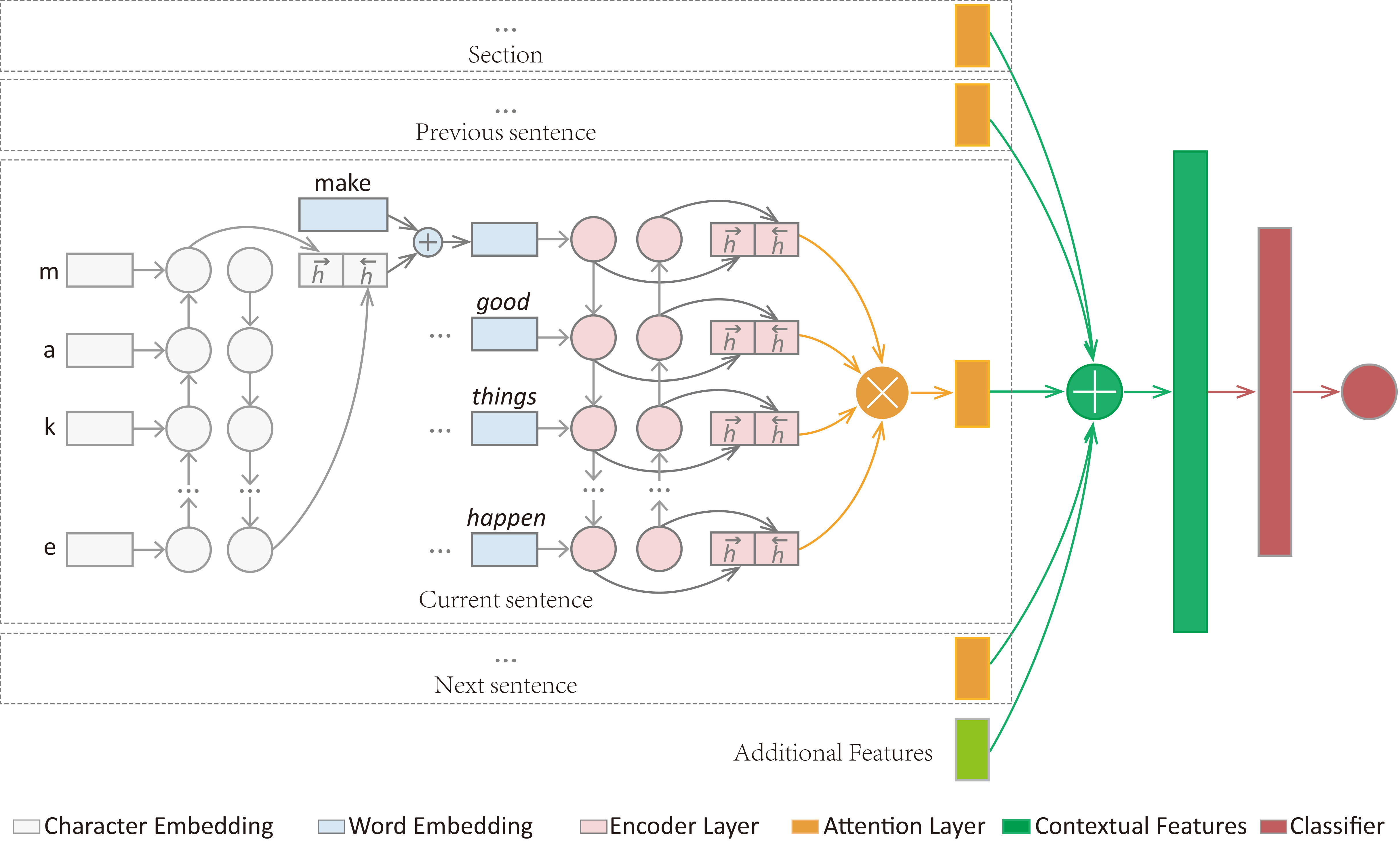
Figure 4: The architecture of the proposed attention-based BiLSTM neural network.

3.1 Character Embedding

In language modeling, it is a common practice to treat a word as the basic unit. Similar to the bag of words assumption, we can consider the text as composed of a bag of characters. santos2014learning, zhangCharacterlevelConvolutionalNetworks2015 and chen2015joint shows that learning a character level embedding could benefit various NLP tasks. In this layer, we get the characters from tokens, then feed the characters to a bidirectional LSTM network, to get a fixed-length representation of the token. By using the character embedding, we can solve the out-of-vocabulary problem for pre-trained word embedding.

3.2 Word Embedding

The word embedding is responsible for mapping a word into a vector of numbers which will be the input for the next layers. For a given sentence $S$, we first convert it into a sequence consisting of $n$ tokens, $S=\{c_{1},c_{2},\cdots,c_{n},\}$ . For each token $c_{i}$, we look up the embedding vector $x_{i}$ from a word embedding matrix $M^{tkn}\in\mathbb{R}^{d|V|}$, where the $d$ is the dimension of the embedding vector and the $V$ is the vocabulary size of the tokens. In this paper, the matrix $M^{tkn}$ is initialized by pre-trained GloVe vectors (pennington2014glove), but will be updated by learning from our corpus. Before feeding the encoder, we concatenate the word vectors from word embedding and character embedding.

3.3 Encoder

Recurrent neural networks (RNNs) are a powerful model to capture features from sequential data, such as temporal series, and text. RNNs could capture long-distance dependency in theory but they suffer from the exploding/vanishing gradient problems (pascanu2013difficulty). This is, as the network is unraveled, the training process becomes chaotic. The Long short-term memory (LSTM) architecture was proposed by hochreiter1997long to solve these issues. LSTM introduces several gates to control the proportion of information to forget from previous time steps and to pass to the next time step. Formally, LSTM could be described by the following equations:

$$i_{t}=\sigma(W_{i}x_{t}+W_{i}h_{t-1}+b_{i})$$ (5)

$$f_{t}=\sigma(W_{f}x_{t}+W_{f}h_{t-1}+b_{f})$$ (6)

$$g_{t}=tanh(W_{g}x_{t}+W_{g}h_{t-1}+b_{g})$$ (7)

$$o_{t}=\sigma(W_{o}x_{t}+W_{o}h_{t-1}+b_{o})$$ (8)

$$c_{t}=f_{t}\bigotimes c_{t-1}+i_{t}\bigotimes g_{t}$$ (9)

$$h_{t}=o_{t}\bigotimes tanh(c_{t})$$ (10)

where the $\sigma$ is the sigmoid function, $\bigotimes$ denotes the dot product, $b$ is the bias, $W$ is the parameters, $x_{t}$ is the input at time $t$, $c_{t}$ is the LSTM cell state at time $t$ and $h_{t}$ is hidden state at time $t$. The $i_{t}$, $f_{t}$, $o_{t}$ and $g_{t}$ are called input, forget, output and cell gates respectively, they control the information to keep in its state and pass to next step.

LSTM gets information from the previous step, which is the context to the left of the current token. However, it is important to consider the information to the right of the current token. A solution of this information need is bidirectional LSTM (graves2013speech). The idea of BiLSTM is to use two LSTM layers and feed in each layer with forward and backward sequences separately, concatenating the hidden states of the two LSTM to model both contexts:

$$h_{t}=[\overrightarrow{h_{t}}\varoplus\overleftarrow{h_{t}}]$$ (11)

For a sentence with $n$ tokens, the hidden state of BiLSTM $H$ would be:

$$H=(h_{1},h_{2},...h_{n})$$ (12)

3.4 Attention

The attention mechanism was introduced for sequence-to-sequence models by bahdanauNeuralMachineTranslation2014. They replace the fixed context vector (produced by the encoder) with a dynamic context vector which is a weighted average of the hidden state of the encoder. The weight of each hidden state is determined by a score between the encoder hidden states and the previous decoder states.

We can consider the previous decoder hidden state as a query vector, the encoder hidden states as key and value vectors. In general, given a query and set of key-value pairs, attention could be interpreted as mapping the query to an output by using the weighted average of the values. The weight to a certain value is computed by a score function of the query with the corresponding key.

Formally, we denote the query as $q$, key as $(k_{1},k_{2},...,k_{n})$ and values as $(v_{1},v_{2},...,v_{n})$, the weigh vector as $(\alpha_{1},\alpha_{2},...,\alpha_{n})$, both of them have same size $n$. the output $z$ is

$$z=\stackrel{{\scriptstyle[}}{{i}}=1]{n}{\sum}\alpha_{i}v_{i}$$ (13)

$$\alpha_{i}=\frac{\exp(\text{score}(q,k_{i}))}{\sum_{i^{{}^{\prime}}=1}^{n}\exp(\text{score}(q,k_{i^{{}^{\prime}}}))}$$ (14)

The weight $\alpha_{i}$ is obtained by using the softmax function, the score($\cdot)$ is a compatibility function between $q$ and $k_{i}$.

There are several score functions, such as additive (bahdanauNeuralMachineTranslation2014) and MLP (linStructuredSelfattentiveSentence2017), however, these methods introduce more parameters to learn. In this paper, we use the cosine ($cos$) score function introduced by graves2014neural, dot-product ($dp$) score function introduced by luongEffectiveApproachesAttentionbased2015 and the scaled dot-product ($sdp$) score function proposed by vaswaniAttentionAllYou2017a. These three approaches are a multiplication of two matrices with no additional hyper-parameters:

$$score_{cos}(q,k)=\frac{q\cdot k}{||q||\text{\textperiodcentered}||k||},$$ (15)

$$score_{dp}(q,k)=qk^{T},$$ (16)

$$score_{sdp}(q,k)=\frac{qk^{T}}{\sqrt{d_{k}}},$$ (17)

where $d_{k}$ is the size of query vector. If there is a scale item, a scalar $\sqrt{d_{k}}$ is applied, otherwise, the dot-product function is applied.

In this research, the query is the hidden state of BiLSTM at the last time step $H$ (see Eq.12) of the encoder. By using the attention mechanism, we effectively use all hidden states, recovering long-distance information dependencies.

3.5 Contextual Features

In this layer, we concatenate the attention output of section, previous sentence, current sentence and next sentence with 8 additional features. The additional features including the character-wise and word-wise sentence length for previous sentence, current sentence and next sentence respectively, and whether previous and next sentence have citation.

3.6 Classifying

The last layer of our model is a classifier layer. The output of attention layer $z$ is passed to a multilayer perceptron and then the softmax function is applied to predict the probability of each class label $\hat{y}$ for a given sentence $S$

$$p(y|S)=\text{softmax}(Wz+b)$$ (18)

$$\hat{y}=\arg\max_{y}\hat{p}(y|S)$$ (19)

We use the cross-entropy loss and L2 regularization as our cost function to maximize the probability of true class label $\hat{y}$:

$$J(\theta)=-\stackrel{{\scriptstyle[}}{{i}}]{N}{\sum}\stackrel{{\scriptstyle[}}{{j}}]{C}{\sum}y_{j}^{(i)}\log\hat{y}_{j}^{(i)}+\lambda||\theta||^{2}$$ (20)

Where $N$ is the total number of the training instances in a batch, $C$ is the number of classes. $y$ is the ground-truth label indicator, $\hat{y}$ is the probability of prediction. $\lambda$ is the amount of L2 regularization, and $\theta$ represent all the trainable parameters.

3.7 Network and training parameters

For all Att-BiLSTM models, we set the dimension of hidden state for character and word embedding to 15 and 128, respectively. We use RELU as the activation function and Adam as the optimizer. We set the learning rate to 0.001 and batch size to 64. In order to avoid over-fitting, we set the dropout rate to 0.5, and also we use L2 regularization of $10^{-7}$. During the training process, if the validation performance does not improve for three epochs, we stop the training and choose the model with best validation performance as the final model.

4 Interpretable models for citation worthiness

In this section, we want to introduce models which offer interpretable results.

Elastic-net Regularized Logistic Regression

The logistic regression model is as follows:

$$p(y_{i}=1)=\sigma(\beta^{T}\mathbf{x}+b),$$ (21)

where $\sigma(z)=(1+e^{-z})^{-1}$, $\beta$ are the weights, $x$ are the inputs, and $b$ is the intercept. If we use normalized terms as features (e.g., tf-idf of uni-grams and bi-grams), we can directly interpret the weights in Eq. 21 to determine whether a term increases the probably of citation or not, and by how much.

Most of the words in our dataset are not predictive of whether a citation is needed. Therefore, we need to reduce the importance of them or remove them from the prediction altogether. Elastic-net regularized logistic regression (ENLR) allows to automatically perform both goals (friedman2001elements). The ENLR loss function has the following form

$$-\left[\sum_{i=1}^{N}y_{i}\cdot\log\sigma(\mathbf{x}_{i})+(1-y_{i})\cdot\log(1-\sigma(\mathbf{x}_{i}))\right]+\lambda\left[\frac{1}{2}\left(1-\alpha\right)||\beta||_{2}^{2}+\alpha||\beta||_{1}\right],$$ (22)

where $\sigma$ is the sigmoid function, $||\beta||_{2}^{2}$ is L2 regularization, and $||\beta||_{1}$ is L1 regularization. The parameter $\alpha$, between 0 and 1, controls how much L1 regularization is added and $\lambda$ controls how much of both regularizers are added to the loss. The parameters $\alpha$ and $\lambda$ are chosen by cross validation.

Random Forest

Elastic-net logistic regression can only find linear relationships between the features $x$ and the output $y$. Random forest is a general method for finding non-linear relationships by using bagging of decision trees. The final decision is made by averaging

$$p(y_{i}=1)=\frac{1}{B}\sum_{j=1}^{B}T_{j}(\mathbf{x}_{i}),$$ (23)

where $T_{j}$ is a decision tree fitted to a subset of the features on a bootstrapped sample of the data. In the case of classification, the final decision is made by majority vote. There are two parameters: the number of trees, $B$, and the number of features to sample for each tree, $p$. Both parameters are chosen by cross validation but typically $p=\sqrt{m}$ where $m$ is the total number of features. Empirical evidence suggests that random forest parameters are robust to overfitting (friedman2001elements).

5 Results

In this work, we examined the factors that lead to a citation being made. We propose a new dataset to answer this question and we proposed a new method based on neural networks to predict which sentences need a citation. We compare this method with several other techniques, and interpret the findings.

5.1 Attention-based BiLSTM model results

We now examine high-performant models that are perhaps less interpretable. We name models using features extracted from the current sentence only as Att-BiLSTM with a subscript. We name models using the features extracted from current sentence and its context as Contextual-Att-BiLSTM with a subscript. The symbol $cos$, $dp$ and $sdp$ represent cosine (Eq. 15), dot-product (Eq. 16) and scaled dot-product (Eq. 17) as the attention score function, respectively.

5.1.1 Results for ACL-ARC dataset

Table 3: Comparison of our Att-BiLSTM models with farber2018cite and bonabCitationWorthinessSentences2018. The hyper-parameters of our models are chosen on the validation set and the performances reported are base on a hold-out testing set.

Model	Precision	Recall	$F_{1}$
CNN GloVe	0.196	0.269	0.227
RNN GloVe	0.171	0.317	0.222
CRNN GloVe	0.182	0.260	0.214
CNN-rnd-update	0.418	0.409	0.413
CNN-w2v-update	0.449	0.406	0.426
Att-BiLSTMsdp	0.766	0.340	0.471
Att-BiLSTMdp	0.711	0.380	0.495
Att-BiLSTMcos	0.720	0.391	0.507

In this section, we first compare our models with the following state-of-art approaches on this task as baselines:

CNN GloVe: a convolutional neural network with GloVe word vector (farber2018cite).

RNN GloVe: a recurrent neural network with GloVe word vector (farber2018cite).

CRNN GloVe: a convolutional recurrent neural network approach proposed by (farber2018cite), using GloVe word vector.

CNN-rnd-update: A CNN-based architecture proposed by bonabCitationWorthinessSentences2018, word embedding are initialized randomly and updated during the training process.

CNN-w2v-update: A CNN-based architecture proposed by bonabCitationWorthinessSentences2018, word embedding are initialized by pre-trained word vectors and updated during the training process. Both of our models and the baselines are evaluated on the same ACL-ARC corpus. In terms of recall, our approaches performs better than models proposed by farber2018cite but lower than models proposed by bonabCitationWorthinessSentences2018. However, in terms of precision, our performance is much better than the baselines. Overall, our results show that our model has significantly higher performance than previous approaches (19% more $F_{1}$). For our models, the cosine score function has notably better performance against the dot-product and scaled dot-product score function, but all of them are better than baselines. As it is revealed by Figure 5, the neural network has find good scores relatively quickly.

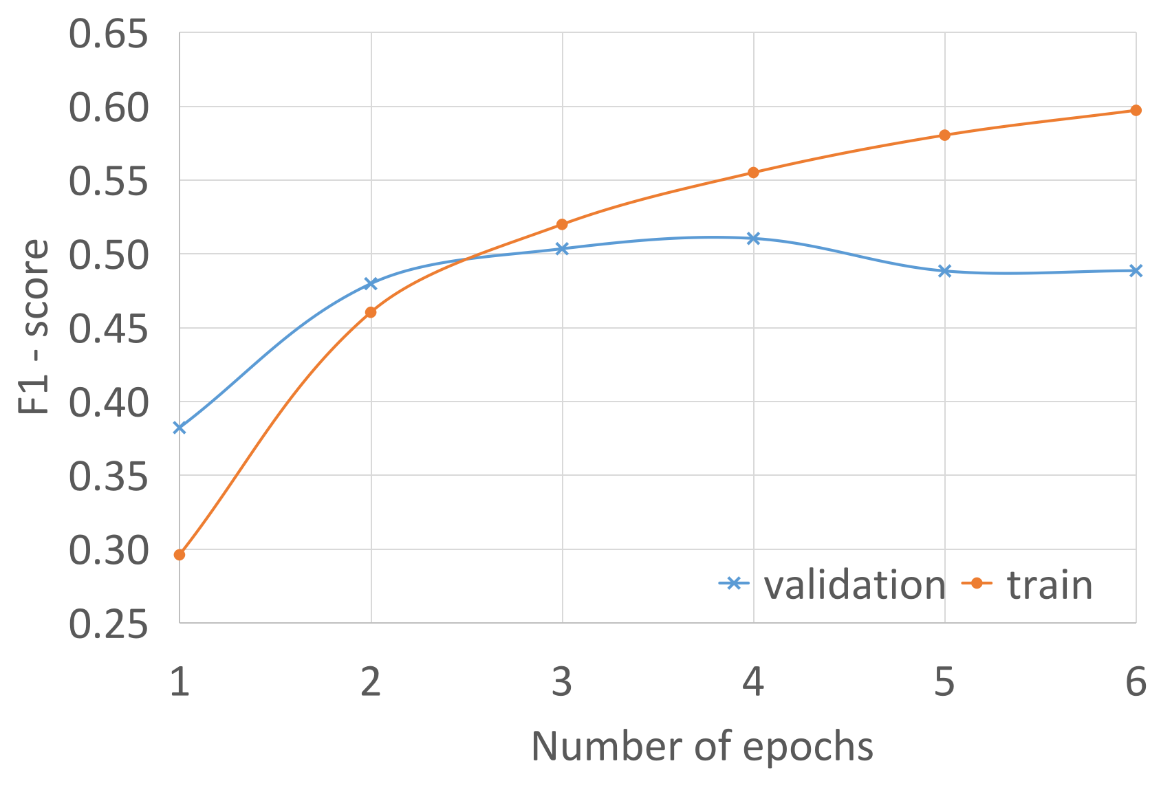
Figure 5: The train and validation $F_{1}$ performance for Att-BiLSTM_cos using ACL-ARC dataset: x-axis shows the number of epoch, the y-axis is $F_{1}$ score.

5.1.2 Results on PubMed Open Access subset dataset (PMOA-CITE)

Table 4: The best performance of models on the PMOAS dataset. The hyper-parameters of our models are chosen on the validation set and the performances reported are based on a hold-out testing set.

Model	Precision	Recall	$F_{1}$
Att-BiLSTMsdp	0.900	0.764	0.827
Att-BiLSTMdp	0.886	0.788	0.834
Att-BiLSTMcos	0.883	0.795	0.837
Contextual-Att-BiLSTMsdp	0.907	0.797	0.848
Contextual-Att-BiLSTMdp	0.908	0.807	0.854
Contextual-Att-BiLSTMcos	0.907	0.811	0.856

We would like to examine how our proposed architecture performs in bio-medical fields with more contextual information added—the previous ACL-ARC dataset does not contain contextual information. The results are presented in Table 4. Similar to before, the cosine attention score function performs best compared with dot product and scaled dot product. This suggests that cosine attention consistently outperforms the two attention score function in different dataset, with or without contextual information. By adding the contextual information, the testing performance improved significantly (e.g. 0.837 to 0.856 in terms of $F_{1}$) across all the different attention types. All our neural network models have much better performance than statistical models discussed below (see Table 7).

When we evaluate the training evolution of Contextual-Att-BiLSTM_cos model (see Figure 6), we found that the first epoch gives enough information to achieve high performance. The validation performance remains relatively stable after two epochs and reaches its peak at the fourth epoch. Overall, our results suggest that deep learning achieves considerable have better performance compared to statistical models.

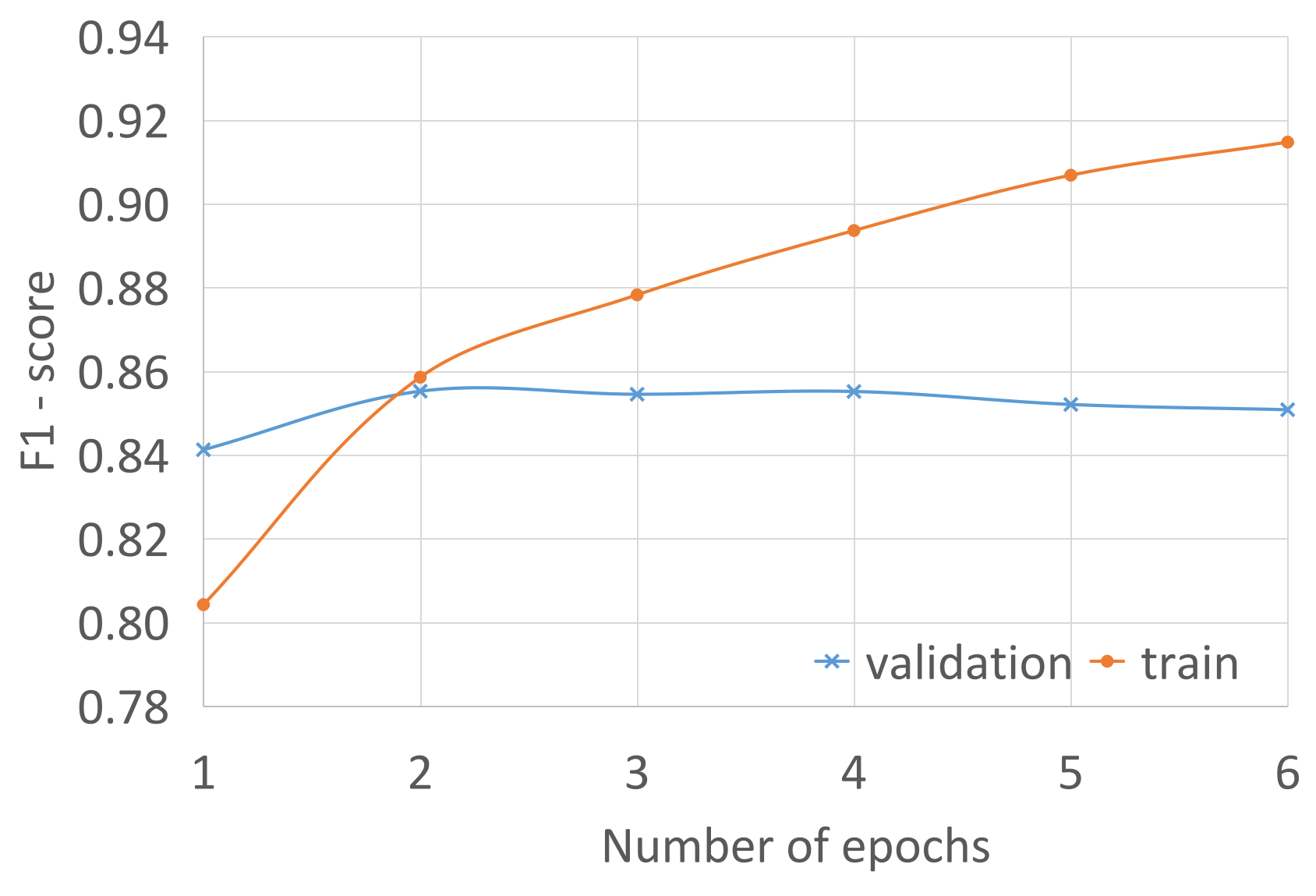
Figure 6: The train and validation $F_{1}$ performance for Contextual-Att-BiLSTM_cos using PMOAS dataset: x-axis shows the number of epoch, the y-axis is $F_{1}$ score.

5.1.3 Down-sampling sensitivity analysis

For most scientific papers, the number of citing sentence $S^{c}$ and non-citing sentences $S^{nc}$ are usually not equal and vary across corpora. Therefore, this issue should be evaluated. In PMOA-CITE, the number of $S^{nc}$ to the number of $S^{c}$ ratio is 4.13. A typical approach to handle unbalanced dataset is to down-sample—reduce the instances of the majority class and keep all the instance of minority class. We investigate how the best architecture found in the previous section (Att-BiLSTM_cos) would perform under these different balance ratios. Importantly, the $S^{nc}$ to $S^{c}$ ratio of held-out dataset remains the same as the natural proportion (4.13), following standard information retrieval practice. Figure 7 shows the performance under the ratios 1, 2, 3, and original 4.13. The results suggest that our model has best performance when the ratio equals the natural proportion. Also, increasing this ratio is associated with an increase in the performance. Therefore, this sensitivity analysis suggest that our model is robust to this kind of down-sampling sensitivity analysis.

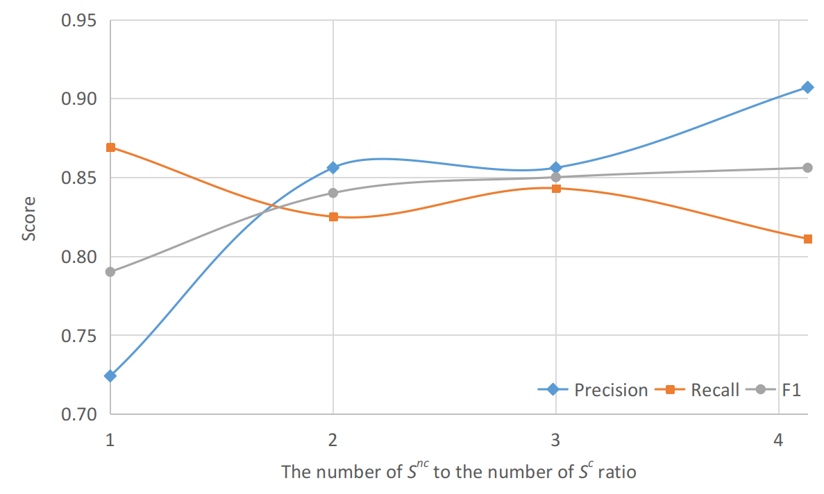
Figure 7: The performance of Att-BiLSTM_cos when the PMOA-CITE dataset is down-sampled. $S^{nc}$ is the number of citing sentences and $S^{c}$ is the number of citing sentences.

5.1.4 Model generalization to different corpora

Transfer learning has become an important topic in AI. Ideally, we would like our model trained on PMOA-CITE, for example, to translate to other datasets. Thus, we experimented with training on PMOA-CITE and estimating performance on ACL-ARC, and vice versa. Expectedly, generalization is hard as models trained and tested on the same dataset have significantly better performance than training on one and evaluation on the other (Table 5). However, the models trained on PMOA-CITE have better cross-dataset generalization performance than those trained on ACL-ARC. We attribute this improvement to the overall quality of this dataset. The ACL-ARC dataset was extracted from PDFs, which induces noise, while PMOA-CITE is already structured with a pre-defined structure (e.g., tag set; see Materials and Methods). Still, generalization is a challenging task.

We also perform experiments on training a model on a combination of PMOA-CITE and ACL-ARC corpora. We matched the amount of data coming from both sources by randomly sampling half from PMOA-CITE and half from ACL-ARC training. Surprisingly, the testing performance on PMOA-CITE and ACL-ARC are more than two times better than previously, and close to the model training and testing solely on one dataset. This suggests a way to solve the generalization problem by training the same model with disparate domains.

Table 5: The performance of model generalization

Architecture	Training $\rightarrow$ Testing corpora	Precision	Recall	$F_{1}$
Att-BiLSTMcosine	ACL-ARC $\rightarrow$ ACL-ARC	0.72	0.391	0.507
Att-BiLSTMcosine	ACL-ARC $\rightarrow$ PMOA-CITE	0.431	0.121	0.189
Att-BiLSTMcosine	PMOA-CITE $\rightarrow$ PMOA-CITE	0.883	0.795	0.837
Att-BiLSTMcosine	PMOA-CITE $\rightarrow$ ACL-ARC	0.155	0.289	0.202
Att-BiLSTMcosine	combined $\rightarrow$ ACL-ARC	0.941	0.669	0.440
Att-BiLSTMcosine	combined $\rightarrow$ PMOA-CITE	0.860	0.765	0.809

5.1.5 Real world applications of our algorithm for publishing

We wanted to examine whether our model can find sentences that seem to be misclassified but actually should have citations. We use the model to make predictions for a hold-out testing set of 201,513 sentences, 3270 of them predicted to be cite worthy. We then manually examine the top 10 sentences by cite worthiness probability (Table 6). Surprisingly, the model discovered some mistakes that we suspect are introduced by scientists or systems processing the accepted manuscripts. These problems can be grouped into three categories. The first category is an XML annotation error. According to the JATS standard, a bibliographic reference in a ref tag should be denoted as a bibr property for ref-type attribute. However, cases numbered 1, 2, 7, and 9 in Table 6 do not comply with this standard and marked as non-citing sentence, but our model detected these sentences should have a citation. A second category contains citations not made properly. In case numbered 8, the author puts an URL at the end of the sentence and therefore the citation is not properly made. The third and perhaps more severe category is mis-citations. For the cases numbered 3, 4, 5 and 10, there are no cross reference annotations in the XML file. However, based on the language, we think it would be better to cite the source of the ideas. An interesting, borderline case outside of this categorization is case 6, which could have a citation but it does not because the authors cited the source somewhere else but felt that citing again would be redundant. In sum, these manually verified cases show that our model could indeed find mistakes. Furthermore, the probability in the prediction could be used as an threshold for warning during pre-submission or during peer review. Thus, our model could be used as a filter for such mistakes before publishing.

Table 6: some mis-citation examples

Case number	Section	Sentence	Probability	Type
1	introduction	The estimated cost of TBI in the United States is $56 billion annually , , with over 1.7 million people yearly suffering from TBI, often resulting in undiagnosed pathology that can lead to chronic disability , .	0.9999	XML annotation error
2	discussion	It has been reported that the inferior turbinate and uncinate process differ dramatically in levels of plasminogen activators and host defense molecules , , .	0.9998	XML annotation error
3	discussion	The importance of hsp90 for CpG ODN-PO–mediated signal transduction is also suggested by Okuya , who recently showed that hsp90 converted inert self-DNA or mainly CpG ODN-PO into potent triggers of IFN-α secretion .	0.9997	mis-citations
4	discussion	The FZP gene and its orthologs in cereals participate in the establishment of floral meristem identity, and fzp mutations affect early events during spikelet development [ ,	0.9996	mis-citations
5	discussion	Most importantly, many of the reporter gene expression assays, specially the one with GFP reporter gene15, may not differentiate between the live and dead intracellular amastigotes.	0.9995	mis-citations
6	intro	Importantly, Kessler and Rutherford found the strongest advantage for visible over occluded responses at 60°, i.e. at the maximum overlap between the avatar’s and the egocentric LoS , reflecting an egocentric influence on processing of the other’s perspective.	0.9994	mentions after citation
7	discussion	B. ovatus has previously been shown to utilize galactomannan as a carbon source , .	0.9994	XML annotation error
8	introduction	More than 600 cry genes have been described (http://www.lifesci.sussex.ac.uk/home/Neil_Crickmore/Bt/toxins2.html).	0.9993	citations not made properly
9	materials and methods	The bioinformatic pipeline used to extract TCRβ sequences was described previously , .	0.9992	XML annotation error
10	discussion	Consistent with previously stated studies, patients who underwent angiography and embolization were reported to have significantly less blood loss during surgery .	0.9992	mis-citations

5.2 Interpretable statistical model results

Statistical learning usually comprises two main parts: prediction and interpretation (James:2014:ISL:2517747). As it is well-known, deep learning provides extremely good prediction performance by trading it off with interpretation. We now explore more interpretable statistical models that can help us understand the language promoting and inhibiting citations worthiness.

5.2.1 Comparison of models and features

We perform experiments using Elastic-net regularized logistic regression (ENLR) and Random Forest (RF) on the bag-of-words (BoW) representation and topic modeling (TM) based representation, with and without contextual information. We first examine the performance of ENLR. In our cross validation, we sweep through a set of regularization parameters ($\lambda$) and L1–L2 mixture parameters ($\alpha$, see Eq. 22). Table 7 shows the test performance for the best cross-validated models across these parameters for different features sets. In general, the BoW representation achieves better overall performance than TM representation; the contextual information improves the performance significantly for both representations. The BoW representation with contextual information gives the best performance ($F_{1}=0.581$).

Table 7: Elastic-net logistic regression (ENLR) model performance

Model	Text representation	Feature set	Precision	Recall	$F_{1}$
$\text{ENLR}_{bow}$	BoW	current sentence	0.461	0.619	0.528
$\text{ENLR}_{bowctx}$	BoW	current sentence + contextual	0.501	0.691	0.581
$\text{ENLR}_{tm}$	TM	current sentence	0.278	0.661	0.392
$\text{ENLR}_{tmctx}$	TM	current sentence + contextual	0.378	0.624	0.471
$\text{RF}_{bow}$	BoW	current sentence	0.402	0.563	0.469
$\text{RF}_{bowctx}$	BoW	current sentence + contextual	0.453	0.637	0.529
$\text{RF}_{tm}$	TM	current sentence	0.281	0.645	0.391
$\text{RF}_{tmctx}$	TM	current sentence + contextual	0.398	0.594	0.477

We then examine the performance of Random Forest, which has the ability to capture non-linear relationships between features. We evaluate RFs with 100, 200, and 500 trees with a parameter sampling strategy that uses the square root of the number of features, $\sqrt{p}$. A number of 500 trees was the best parameter for both BoW and topic modeling. Table 7 shows the best performance across these parameters on testing. The results suggest that, in contrast to ENLR, RF performs best with BoW ($F_{1}=0.529$) representation while TM representation has a lower performance ($F_{1}=0.477$). As with ENLR, the topic models had the worst performance ($F_{1}=0.391$) and the contextual information promotes the performance notably for both representations.

5.2.2 Word importance in the prediction

Interpretation usually combines two steps: extraction of the important features and the direction of influence of those features. For example, we would like to know which words are most related to the presence or absence of citations (e.g., feature importance) and which of these words promotes (positive sign) or inhibits (negative sign) citation worthiness. We get the feature importance from the random forest model and the direction of the influence from an elastic net regularized logistic regression model. Feature importance across all the features sum up to one: the larger the feature importance, the more it affects the model. Therefore, random forest and logistic regression can be combined for the two steps necessary for interpretation.

First, we analyze the features at a high level by evaluating the combined importance of terms. We sum the feature importance of all uni-grams and bi-grams to form a category for the section type and current and contextual sentences. In this manner, we know the overall influence of these components before understanding the importance of the terms they contain. This analysis shows that target sentence plays the most import role (Table 8), followed by next sentence and the section. The previous sentence has the smallest impact. It is worth noting that the feature importance of current sentence is more than 4.86, 4.94 4.30 times important than section type, previous sentence and next sentence, respectively. However, as the performance of the models showed above, still the context contributes significant performance advantages. Also, we found that the more characters or words a sentence has, the more likely the sentence needs a citation (Table 8 ). For individual features, the presence of a citation in previous and next sentences has significant positive impact on citation worthiness.

We wanted to understand how the section relates to citation worthiness. Table 9 shows the 10 most positive and 10 most negative weights of the section type. The positive terms in the section type are related to background information and discussion (e.g. “introduction”, “background”, “discussion”) where scientific papers usually describe previous work to contextualize the research being reported. In contrast, the negative terms are related to descriptions and reports (e.g. “results”, “methods”, “materials”), therefore lowering the probability to have a citation. Thus, this shows that the section can be have different influences on citation worthiness.

We also wanted to investigate which uni-grams and bi-grams in the current sentence relates to the citation worthiness. The positive words are intuitive as they relate to describing events from the past (e.g., "previously", "previous", "recently") and mentioning other studies (e.g., "reported", "described", "been demonstrated" ). Negative terms refer to the current paper (e.g., "this study", "the study"), entities which do not need a citation (e.g., floating elements: "figure", "table"; statistics: "min", "mean", "test"; proper names: "usa", "cells were"), and descriptive languages of experiments or actions taken within the paper (e.g,. "washed", "incubated"). Therefore, uni-grams and bi-grams and their weights reveal interesting patters about the presence or absence of a citation.

Table 8: Feature importance for BoW representation. All the feature importance sum up to 1. The plus sign (+) means the feature has a positive influence on the citation worthiness. The minus sign (-) means the feature has a negative influence on the citation worthiness.

Category	Importance	Sign of Influence
sum of term importance of section type	0.11627	N/A
sum of term importance of $S_{n-1}$	0.10967	N/A
number of characters in $S_{n-1}$	0.00279	+
number of words in $S_{n-1}$	0.00191	+
sum of term importance of $S_{n}$	0.54243	N/A
number of characters in $S_{n}$	0.01061	+
number of words in $S_{n}$	0.01230	+
sum of term importance of $S_{n+1}$	0.11840	N/A
number of characters in $S_{n+1}$	0.00803	+
number of words in $S_{n+1}$	0.00492	+
similarity between $S_{n-1}$ and $S_{n}$	0.00566	-
similarity between $S_{n+1}$ and $S_{n}$	0.00694	-
whether $S_{n-1}$ has citation	0.02461	+
whether $S_{n+1}$ has citation	0.03545	+

Table 9: Term (uni-gram or bi-gram) importance of the section type. The plus sign (+) means the feature has a positive influence on the citation worthiness. The minus sign (-) means the feature has a negative influence on the citation worthiness.

Term in Section Type	Feature Importance	Sign of Influence
introduction	0.027079	+
intro	0.015247	+
background	0.008828	+
discussion	0.003698	+
cancer	0.00155	+
mechanisms	0.001328	+
cells	0.000695	+
role	0.000562	+
cell	0.000521	+
receptors	0.000379	+

Term in Section Type	Feature Importance	Sign of Influence
results	0.0174270	-
methods	0.0128930	-
materials	0.0059190	-
case	0.0024290	-
report	0.0014750	-
experimental	0.0010170	-
authors	0.0008160	-
conclusion	0.0007460	-
presentation	0.0006070	-
contributions	0.0006050	-

Table 10: Term importance of current sentence. The plus sign (+) means the feature has a positive influence on the citation worthiness. The minus sign (-) means the feature has a negative influence on the citation worthiness.

Term in Section Type	Feature Importance	Sign of Influence
previously	0.020892	+
has been	0.015886	+
reported	0.013642	+
previous	0.012692	+
studies	0.011627	+
been reported	0.010001	+
shown that	0.009809	+
have been	0.009625	+
reported that	0.009573	+
previously described	0.009507	+
described	0.009468	+
recently	0.008796	+
recent	0.008359	+
been shown	0.007396	+
studies have	0.006598	+
previous studies	0.006528	+
described previously	0.004926	+
associated with	0.00485	+
been demonstrated	0.004735	+
known	0.004124	+

Term in Section Type	Feature Importance	Sign of Influence
figure	0.00224	-
table	0.002148	-
fig	0.001865	-
samples	0.001642	-
participants	0.001423	-
cells were	0.001363	-
this study	0.001358	-
pbs	0.001152	-
min	0.000894	-
the study	0.000816	-
washed	0.000812	-
mean	0.00072	-
test	0.00072	-
groups	0.000699	-
difference	0.000698	-
for min	0.000673	-
sample	0.00066	-
total	0.000613	-
incubated	0.000606	-
usa	0.000573	-

5.2.3 Topic importance in the prediction

In the section, we want to examine how the topic relates to citation worthiness. Similar to above, we get the feature importance from random forest model and the direction of feature influence from elastic net regularized logistic regression model. We sum the feature importance of all topics to form a category for the section type and current and contextual sentences. As Table 11 shows, the current sentence has the largest impact on citation worthiness. It is 2.06, 1.83 and 1.80 times more important than section type, previous sentence and next sentence, respectively. Similar to the BoW representation, the presence of citation in previous and next sentence plays an import role as they are the top 2 most import features across all the features.

Table 11: Feature importance for topic modeling representation. All the Feature Importance sum to 1. he plus sign (+) means the feature has a positive influence on the citation worthiness. The minus sign (-) means the feature has a negative influence on the citation worthiness.

Category	Importance	Sign of Influence
sum of topic importance of section type	0.16323	N/A
sum of topic importance of $S_{n-1}$	0.18016	N/A
number of characters in $S_{n-1}$	0.00243	+
number of words in $S_{n-1}$	0.00185	-
sum of topic importance of $S_{n}$	0.31768	N/A
number of characters in $S_{n}$	0.00947	-
number of words in $S_{n}$	0.01049	+
sum of topic importance of $S_{n+1}$	0.18135	N/A
number of characters in $S_{n+1}$	0.00377	+
number of words in $S_{n+1}$	0.00223	-
similarity between $S_{n-1}$ and $S_{n}$	0.00272	-
similarity between $S_{n+1}$ and $S_{n}$	0.00327	-
whether $S_{n-1}$ has citation	0.05891	+
whether $S_{n+1}$ has citation	0.06244	+

In order to understand a topic, we extracted all the terms and their weights from the trained LDA model. The term weights for a topic are a probability distribution and therefore sum up to 1. The large the weight, the more important the term in the topic.

As Table 12 shows, all the topics in section type contribute positively to citation worthiness. The most representative terms in each topic are methods, introduction, conclusions and results. Across topics, there are some inflectional forms of a word a word (e.g., “materials”, “material”). This is because most section types are just one word, offering little information to LDA.

Table 12: Topic importance of the section type

Topic Number	Importance	Sign	Weights of Topic Terms
1	0.0588	+	Terms	methods	materials	case	report
			Term Weights	0.2155	0.1724	0.0199	0.0175
2	0.0477	+	Terms	introduction	background	authors	contributions
			Term Weights	0.1239	0.0552	0.0114	0.0091
0	0.0330	+	Terms	conclusions	material	study	method
			Term Weights	0.0633	0.0148	0.0114	0.0110
3	0.0238	+	Terms	results	discussion	intro	experimental
			Term Weights	0.1998	0.1911	0.0714	0.0302

We then further investigate the topic importance of the current sentence. Table 13 shows the three most important positive and negative topics, with some arbitrary identifier. The most important topic, topic 80 is represented by the terms describing previous work. The second most important topic, topic 108 is represented by bio-medical terms. Finally, topic 82 refers to methods and tools. The importance of topic 80 doubles that of topics 108 and 82. This suggests, similar to our BoW analysis above, that terms describing previous work is highly related to citation worthiness. Conversely, the most negative topics are 150, 122 and 179, and they all have similar importance. These topics describe entities within the same paper, (e.g., “test”, “fig”) which usually do not require citations. Therefore, positive and negative topics have a great deal of interpretability.

Table 13: Topic importance of target sentence

Topic Number	Importance	Sign	Topic Terms
80	0.0115	+	Terms	described	previously	method	determined
			Term Weights	0.0998	0.0830	0.0719	0.0640
108	0.0055	+	Terms	cells	cell	induced	following
			Term Weights	0.1009	0.0680	0.0319	0.0296
82	0.0052	+	Terms	usa	analyses	version	spss
			Term Weights	0.1331	0.0802	0.0717	0.0367
150	0.0063	-	Terms	test	fig	analyzed	post
			Term Weights	0.0853	0.0690	0.0466	0.0428
122	0.0043	-	Terms	buffer	constant	nacl	contribution
			Term Weights	0.0936	0.0544	0.0368	0.0361
179	0.0036	-	Terms	university	approved	minutes	committee
			Term Weights	0.0658	0.0618	0.0514	0.0423

6 Discussion

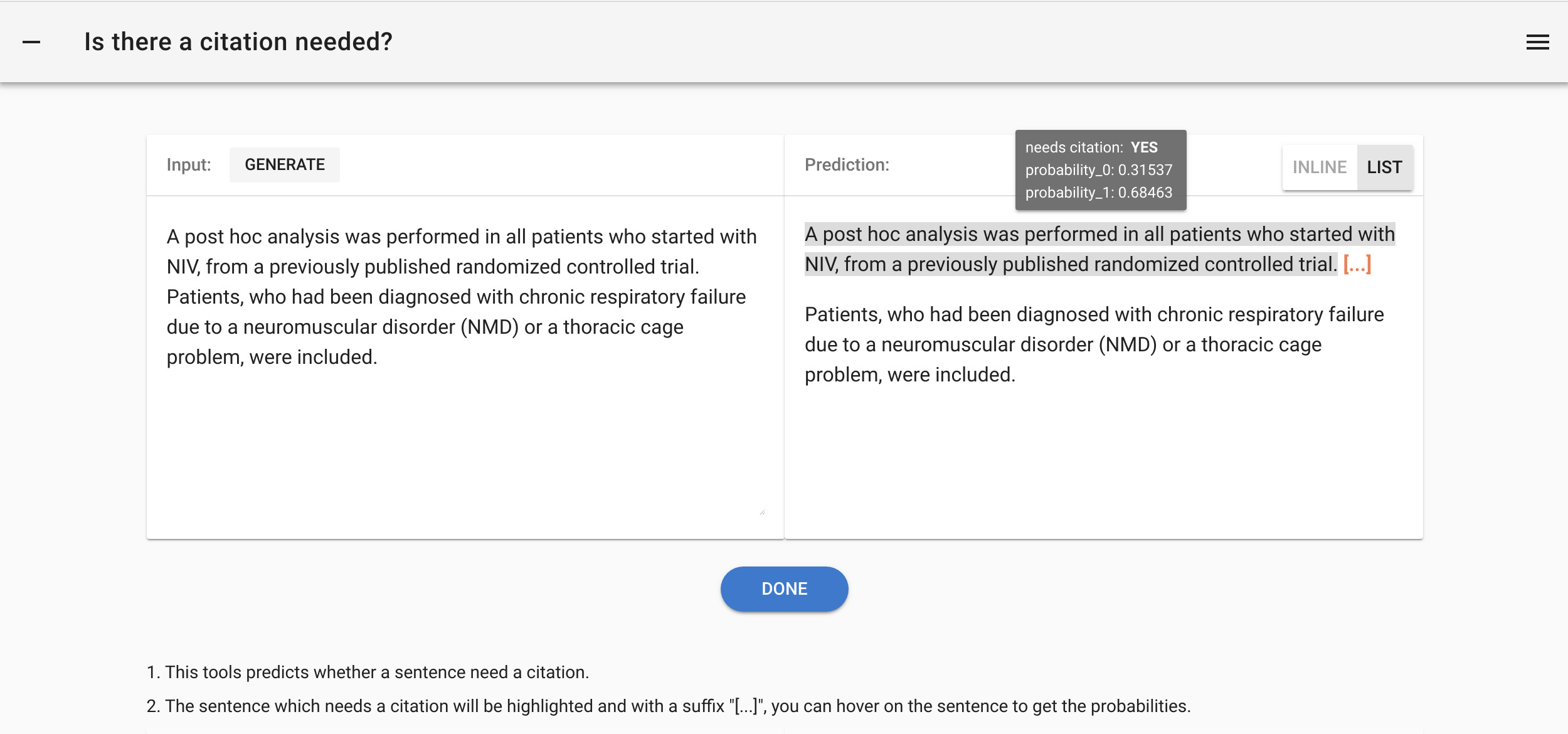
Figure 8: A screenshot of the online predicting tool

In this work, we developed methods and a large dataset for improving the detection of citation worthiness. Citation worthiness is an important first step for constructing robust and well-structured arguments in science. It is crucial for determining where sources of ideas should mentioned within a manuscript. Previous research has shown promising results but thanks to our new large dataset and modern deep learning architecture, we were able to achieve significantly good performance. We additionally proposed several techniques to interpret what makes scientists use citations. We uncovered potential issues in citation data and behavior: XML documents not properly tagged, citations in the wrong form, and, even worse, scientists failing to cite when they should have. We make our code and a web-based tool available for the scientific community. Our results and new datasets should contribute to the larger need to complement scientific writing with automated techniques. Taken together, our results suggest that deep learning with modern attention-based mechanisms can be effectively used for citation worthiness. We now describe contributions in the context of other work and potential limitations of our approach.

The experimental results show that our proposed attention-based BiLSTM architecture can effectively learn from the data. Compared with previous state-of-art, our approach has significantly better performance ($F_{1}(\text{Att-BiLSTM}_{cos})=0.507$ vs $F_{1}(\text{CNN-w2v-update})=0.426$) in Table 3. We attribute the improvements to: 1) The character embedding providing extra information, 2) the effectiveness of the BiLSTM network to capture sequential patterns in sentences, and 3) the attention mechanism helping to generate better representations. When compared with interpretable statistical models, our deep learning architecture has a large improvement in $F_{1}$ (0.856 vs 0.581). This shows that the deep learning architecture was better than the classical methods in terms of performance, but at the cost of interpretability. Recent work by (linStructuredSelfattentiveSentence2017; bahdanauNeuralMachineTranslation2014), however, shows promising visualization techniques for attention mechanisms that could improve deep learning interpretability for this task. Taken together, our results suggest that deep learning with modern attention-based mechanisms can be effectively used for citation worthiness.

As an enhancement to the ACL-ARC dataset, we proposed the PMOA-CITE dataset in the hope of facilitating research on the citation worthiness task. This extends the datasets available to the field of bio-medical science. Our improvements are 1) a two orders of magnitude increase in data size, 2) a well-structured XML file that is less noisy, and 3) contextual information. This dataset could be potentially used in other citation context-related research, such as text summarization (chen2019automatic), or citation recommendation (HuangNeuralProbabilisticModela). Therefore, our contribution goes beyond the application of citation worthiness.

Based on the experiments on PMOA-CITE dataset, the use of contextual features consistently improved the performance. This improvement was independent of the algorithm and text representation used (Tables 4 and 7) . A similar results was reported in HeContextawareCitationRecommendation2010 and jochim2012towards). This suggests that contextual information was key for citation worthiness and other related tasks.

The results of interpretable models reveal interesting patterns about language use in citation worthiness. As suggested by writing guides (e.g., booth2016craft), researchers usually develop their ideas based on several sources, which they quote, paraphrase, or summarize and should therefore cite properly. Otherwise, the paper could lose the trust of the readers, or even worse, run into suspicion of plagiarism (masic2013importance). Our interpretation of feature importance discovered some patterns of language usage for quoting, paraphrasing or summarizing, and it real world applications could help to understanding when a citation should be placed automatically. Also, the terms discovered could help as educational resource for scientific writing. The interpretable models then recognize systematic patterns of citations that are worth exploring.

To the best of our knowledge, Table 5 was the first domain generalization performance reported for this task. While the generalization was poor, this exercise highlights importance of the domain knowledge to this task and showed the difficulty for domain generalization. Our experiment showed that learning from multiple source domains could promote the generalization on unseen target domains. Thus, the release of our dataset can help in this endeavor.

In order to facilitate future research, we made our datasets and models available to the public. The links of the dataset and the code parsing XML files are available at https://github.com/sciosci/cite-worthiness . We also built a web-based tool (see Figure 8) at http://cite-worthiness.scienceofscience.org. This tool might help inform journalist, policy makers, the public to better understand the principles of proper source citation and credit assignment.

We now discuss some of the limitations of our work. Our proposed deep learning architecture is computational costly. We had to limit data sample size used from our proposed dataset, and also we had to limit the hyper-parameter search due to time constraints. These limitations are mainly due to the RNN component of the architecture, whose encoding and sequential nature were difficult to parallelize. One possible solution to this problem could be the transformer network proposed by vaswaniAttentionAllYou2017a, because it eliminates recurrence entirely, making it more parallelizable. However, it is unclear whether the transformer could improve memory usage. Our validation performance as a function of epochs, however, showed that the model was able to learn relatively quickly, making it unclear whether more data would significantly improve this already good performance (Fig. 6). In the future, we will investigate optimizations to our architecture to improve its memory and time consumption.

When extracting the contextual features, we used previous sentence and next sentence statically. However, there could be longer term dependencies (e.g., information more than one sentence away) that, when not included, incurred in contextual information loss. Conversely, if the surrounding sentences truly were not semantically related to the current sentence, adding them to the prediction could only produce noise. As previously reported by kang2012characteristics, only 5.2% citations are multi-sentence. Although our approach has some limitations, it still covers most situations and simplifies the problem. To solve this, a possible solution could be identify the sentences that are closely related to current sentence dynamically (kaplan2016citation; fetahufine; jebari2018new). We will explore this approach in the future.

Our approach was primarily developed with scientific articles from bio-medical sciences in mind. Therefore, generalization to other domains, such as news or general public pieces, can be severely limited. Scientific writing might not be reflective of how journalists or other people write other types of text. Science has a well-established set of rules for adding citations, perhaps making the data “too clean.” Future work will cross validate our results with general venues such as Wikipedia (e.g., see chen2012citation).

There are several avenues for future research. We can first investigate how to recommend citations automatically based on the target sentence and its context. This work offers the probability of a sentence need a citation, thus forms an important step in this direction. In the larger context of this research, there is a need to appropriately cite credible sources. The research proposed here only addresses a small portion of this challenge: while citation mistakes have been estimated to be surprisingly prevalent—more than 20% of citations are wrong (lukic2004citation; mogull2017accuracy)—we believe that scientists tend to cite credible sources and they unintentionally mis-cite. However, the problem is much more complex in other areas such as fake news. These types of articles do cite sources but the sources are not credible or taken out of context (allcott2017social). Studies on detecting the credibility and quality of sources is a much more complex problem which forms a challenging future research program.

7 Conclusion

In this article, we use open access scientific publications to detect which sentences need citations. In particular, we build an deep learning model based on attention mechanism and BiLSTM which achieve the state of art performance while we also build models offering good interpretability. We make the dataset, the model, and a web-based tool openly available to the community. Our work therefore is an important step to improve the quality of information and provide a data-driven tool to study citations in science. We therefore hope that our work creates more systematic studies regarding citation worthiness as it is the first and crucial step for several tasks to make science more robust and well-structured.

8 Acknowledgments

Tong Zeng was funded by the China Scholarship Council #201706190067. Daniel E. Acuna was partially funded by the National Science Foundation awards #1800956.