Linearized gravity and soft graviton theorem in de Sitter spacetime

Linearized gravity and soft graviton theorem in de Sitter spacetime

Pujian Mao and Bochen Zhou

Abstract. We study the linearized gravity theory in the Newman-Unti gauge in the near horizon region of the de Sitter spacetime. The linearized Einstein equation involves the cosmological constant. The near horizon symmetry consists of near horizon supertranslation and near horizon superrotation. We compute the near horizon supertranslation charge and find the proper near horizon fall-off conditions which uncover a soft graviton theorem from the Ward identity of the near horizon supertranslation.

Emails: pjmao@tju.edu.cn,  zhoubch@tju.edu.cn

1 Introduction

Black holes are recently shown to carry soft hairs [1] which reveals a much richer structure that black holes can have. The new degrees of freedom are labelled by the near horizon symmetries [2, 3, 4, 5, 6, 7, 8, 9, 10, 11, 12, 13, 14, 15, 16, 17, 18, 19, 20, 21, 22, 23, 24, 25, 26, 27, 28, 29, 30, 31, 32]. Black hole horizons can be considered as inner boundary of the spacetime which share many common features as the null infinity, see, e.g., investigations in [33, 34]. At null infinity, a triangle equivalence was proven [35] which connects asymptotic symmetry, memory effect, and soft theorem. Inspired by the null infinity triangle relation, black hole memory effect was subsequently proposed [36, 37, 38, 26] and it is closely related to the near horizon symmetry. Another branch following the triangle relation is the soft theorems relevant to near horizon symmetry which have been investigated for Schwarzschild black hole [39, 40, 41]. Nevertheless, horizons are not exclusive to black holes. The expanding universe leads to cosmological horizons which are locally very similar to the black hole horizon. Soft theorems of gauge theory in de Sitter (dS) spacetime are obtained from the near horizon symmetry [42]. The computations in [42] are somewhat similar to the Schwarzschild case [39, 40]. While, the physical motivation and consequence are very different. Cosmological horizon is the outer boundary of inside observer. Because the dS cosmological universe is expanding so fast, there are events which will never be seen by an observer inside. Considering the fact that we do live in an expanding universe, the near cosmological horizon analysis can be intuitively understood as the real world asymptotic analysis near null infinity. Technically, there is well defined flat limit from the cosmological solution [43, 44, 45]. In the flat limit, the cosmological horizon becomes the null infinity. Correspondingly, the soft theorems derived in dS spacetime do recover the flat spacetime ones [42]. The aim of the present work is to extend the previous study [42] in dS spacetime to linearized gravity.

For the linearization of Einstein theory in dS spacetime, the linearized equations of motion also involve the cosmological constant, see, e.g., [46, 47, 48]. This is the main technical difference than previous studies, e.g., linearized gravity in Schwarzschild spacetime [41] or gauge theories in dS spacetime [42]. Now the cosmological constant arises from both the background spacetime and the perturbative equations of motion. Hence, it is very questionable that if the nice structure revealed in [41] or [42] can be derived for linearized gravity in dS spacetime.

In this work, we apply the Newman-Unti (NU) gauge [49] for the linearized gravity theory in dS spacetime. In the near cosmological horizon region, we impose traceless fall-off conditions. We compute the near horizon symmetry which consists of near horizon supertranslation and near horizon superrotation. The near horizon solution space is specified and the supertranslation charge is derived. We find that there is an interesting reduction of the near horizon solution space which is invariant under supertranslation and leads to a natural split of the supertranslation charge into soft and hard parts. We found such configuration for the Schwarzschild black hole case in previous work [41] and considered that as a coincidence. Now such configuration also arises for the dS spacetime. This may suggest that there is a common structure in the near horizon region which is subject to a soft theorem. A soft graviton theorem in coordinate space is derived from the Ward identity of the near horizon supertranslation in the reduced solution space. After transforming the soft graviton theorem into the momentum space, there is a natural flat limit and it recovers the flat space soft graviton theorem.

This paper is organized as follows. In the next section, we present the linearized Einstein equation in dS spacetime, compute the near horizon symmetry and solution space of the linearized theory. We specify a reduction of the solution space where the supertranslation charge can split into a soft piece and a hard piece. In section 3, a soft graviton theorem is derived from the Ward identity of the near horizon supertranslation charge. The soft theorem has a desired flat limit in the momentum space. The last section is devoted to conclusion and discussion. There is one Appendix which presents the details of the modification of the stress tensor that coupled to the gravity theory.

2 Near horizon symmetries and charges

In this section, we will study the linearized Einstein theory in the dS spacetime. The NU gauge [49] (see also [50, 51]) will be adapted into the linearized theory. We will perform the standard near horizon analysis. The near horizon symmetry, solution space, and surface charge will be computed.

2.1 Near horizon form of the dS spacetime in NU gauge

We start from the static patch in dS spacetime, which is part of the full dS spacetime as shown in Fig. 1.

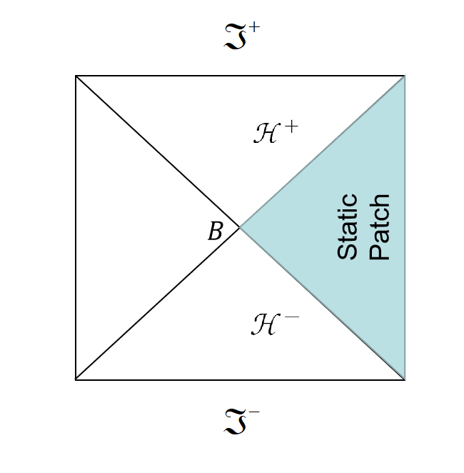
Figure 1: Penrose diagram of de Sitter spacetime

In static coordinates $(t,r,z,\bar{z})$, the line element of the dS spacetime is

$$\mathrm{d}s^{2}=-F(r)\mathrm{d}t^{2}+F(r)^{-1}\mathrm{d}r^{2}+2\Omega(r)^{2}\gamma_{z\bar{z}}\mathrm{d}z\mathrm{d}\bar{z}\,,$$ (1)

$$F(r)=\frac{2r}{\ell}-\frac{r^{2}}{\ell^{2}}\,,\qquad\Omega=\ell-r\,,\qquad\gamma_{z\bar{z}}=\frac{2}{(1+z\bar{z})^{2}}\,,$$ (2)

where $\ell$ is the dS radius and it is related to the cosmological constant by $\Lambda=\frac{3}{\ell^{2}}$. Note that we have set the cosmological horizon at $r=0$. By introducing the retarded time coordinate $u=t-\frac{1}{2}\ell\log\left(\frac{r}{2\ell-r}\right)$, the line element can be written as

$$\mathrm{d}s^{2}=\bar{g}_{\mu\nu}\text{d}x^{\mu}\text{d}x^{\nu}=-F(r)\mathrm{d}u^{2}-2\mathrm{d}r\mathrm{d}u+2\Omega(r)^{2}\gamma_{z\bar{z}}\mathrm{d}z\mathrm{d}\bar{z}\,,$$ (3)

which covers only the $\mathcal{H}^{-}$ part of the horizon. A similar analysis could be performed for $\mathcal{H}^{+}$ simply by a time reverse transformation of dS spacetime near the bifurcation sphere $B$. In the rest of this paper, we just focus on the $\mathcal{H}^{-}$ part.

2.2 Linearization in dS spacetime

We linearize Einstein theory in dS spacetime (3). The metric expands as $g_{\mu\nu}=\bar{g}_{\mu\nu}+\kappa h_{\mu\nu}$. The inverse metric is $g^{\mu\nu}=\bar{g}^{\mu\nu}-\kappa h^{\mu\nu}+{\cal O}(\kappa^{2})$, where the indices are now raised by $\bar{g}^{\mu\nu}$. Up to the first correction order ${\cal O}(\kappa)$, the connection is given by

$$\Gamma^{\alpha}_{\mu\nu}={\bar{\Gamma}}^{\alpha}_{\mu\nu}+\frac{\kappa}{2}\bar{g}^{\alpha\beta}\left(\bar{\nabla}_{\mu}h_{\nu\beta}+\bar{\nabla}_{\nu}h_{\mu\beta}-\bar{\nabla}_{\beta}h_{\mu\nu}\right).$$ (4)

We define

$$C^{\alpha}_{\mu\nu}=\bar{g}^{\alpha\beta}\left(\bar{\nabla}_{\mu}h_{\nu\beta}+\bar{\nabla}_{\nu}h_{\mu\beta}-\bar{\nabla}_{\beta}h_{\mu\nu}\right),$$ (5)

which is very useful for the computation of the curvature tensor,

$${R_{\mu\nu\alpha}}^{\beta} =\partial_{\nu}\Gamma^{\beta}_{\mu\alpha}-\partial_{\mu}\Gamma^{\beta}_{\nu\alpha}+\Gamma^{\tau}_{\mu\alpha}\Gamma^{\beta}_{\nu\tau}-\Gamma^{\tau}_{\nu\alpha}\Gamma^{\beta}_{\mu\tau}$$

$$={\bar{R}_{\mu\nu\alpha}}^{\quad\,\,\,\beta}+\frac{\kappa}{2}(\bar{\nabla}_{\nu}C^{\beta}_{\mu\alpha}-\bar{\nabla}_{\mu}C_{\nu\alpha}^{\beta})+{\cal O}(\kappa^{2})$$ (6)

$$={\bar{R}_{\mu\nu\alpha}}^{\quad\,\,\,\beta}+\frac{\kappa}{2}\bar{\nabla}_{\nu}\left(\bar{\nabla}_{\mu}h^{\beta}_{\alpha}+\bar{\nabla}_{\alpha}h_{\mu}^{\beta}-\bar{\nabla}^{\beta}h_{\mu\alpha}\right)$$

$$\hskip 56.9055pt-\frac{\kappa}{2}\bar{\nabla}_{\mu}\left(\bar{\nabla}_{\nu}h^{\beta}_{\alpha}+\bar{\nabla}_{\alpha}h_{\nu}^{\beta}-\bar{\nabla}^{\beta}h_{\nu\alpha}\right)+{\cal O}(\kappa^{2}).$$ (7)

The Ricci tensor is defined from the curvature tensor as

$$R_{\mu\alpha}={R_{\mu\nu\alpha}}^{\nu}=\bar{R}_{\mu\alpha}+\frac{\kappa}{2}\bar{\nabla}_{\nu}\left(\bar{\nabla}_{\mu}h^{\nu}_{\alpha}+\bar{\nabla}_{\alpha}h_{\mu}^{\nu}-\bar{\nabla}^{\nu}h_{\mu\alpha}\right)-\frac{\kappa}{2}\bar{\nabla}_{\mu}\bar{\nabla}_{\alpha}h_{\nu}^{\nu}+{\cal O}(\kappa^{2}).$$ (8)

Finally, the Ricci scalar is obtained as

$$R=g^{\mu\alpha}R_{\mu\alpha}=\bar{R}-\kappa h^{\mu\alpha}\bar{R}_{\mu\alpha}+\frac{\kappa}{2}\bar{\nabla}_{\nu}\left(\bar{\nabla}_{\mu}h^{\nu\mu}+\bar{\nabla}^{\mu}h_{\mu}^{\nu}-\bar{\nabla}^{\nu}h_{\mu}^{\mu}\right)-\frac{\kappa}{2}\bar{\nabla}_{\mu}\bar{\nabla}^{\mu}h_{\nu}^{\nu}+{\cal O}(\kappa^{2}).$$ (9)

We consider Einstein equation with a cosmological constant $\Lambda=\frac{3}{\ell^{2}}$,

$$R_{\mu\nu}-\frac{1}{2}g_{\mu\nu}R+\frac{3}{\ell^{2}}g_{\mu\nu}=T_{\mu\nu},$$ (10)

where we use the natural unit $8\pi G_{N}=1$. At the linearized order ${\cal O}(\kappa)$, Einstein equation is reduced to

$$E_{\mu\nu}\equiv\frac{1}{2}\left[\bar{\nabla}_{\tau}\bar{\nabla}_{\mu}h^{\tau}_{\nu}+\bar{\nabla}_{\tau}\bar{\nabla}_{\nu}h^{\tau}_{\mu}-\bar{\nabla}^{2}h_{\mu\nu}-\bar{\nabla}_{\mu}\bar{\nabla}_{\nu}h\right]\\ -\frac{1}{2}\bar{g}_{\mu\nu}\left(\bar{\nabla}_{\alpha}\bar{\nabla}_{\beta}h^{\alpha\beta}-\bar{\nabla}^{2}h\right)-\frac{3}{\ell^{2}}h_{\mu\nu}+\frac{3}{2\ell^{2}}\bar{g}_{\mu\nu}h=T_{\mu\nu},$$ (11)

where we apply the relations from the Einstein equation of the dS spacetime

$$\bar{R}_{\mu\nu}=\frac{3}{\ell^{2}}\bar{g}_{\mu\nu},\quad\quad\bar{R}=\frac{12}{\ell^{2}},$$ (12)

and $h=\bar{g}^{\mu\nu}h_{\mu\nu}$. The linearized equation (11) is invariant under the gauge transformation

$$h_{\mu\nu}\rightarrow h_{\mu\nu}+\bar{\nabla}_{\mu}\xi_{\nu}+\bar{\nabla}_{\nu}\xi_{\mu}.$$ (13)

To verify the gauge invariance, the following relations of the dS spacetime are applied,

$$(\bar{\nabla}_{\mu}\bar{\nabla}_{\nu}-\bar{\nabla}_{\nu}\bar{\nabla}_{\mu})\xi_{\alpha}={\bar{R}_{\mu\nu\alpha}}^{\quad\,\,\,\beta}\xi_{\beta},\quad\quad\bar{R}_{\mu\nu\alpha\beta}=\frac{1}{\ell^{2}}(\bar{g}_{\mu\alpha}\bar{g}_{\nu\beta}-\bar{g}_{\mu\beta}\bar{g}_{\nu\alpha}).$$ (14)

2.3 Near horizon symmetries in NU gauge

We will work in the adapted NU gauge for linearized theory [51] where the following conditions are imposed,

$$h_{rr}=h_{rz}=h_{r\bar{z}}=h_{ru}=0\,,$$ (15)

$$T_{rr}=T_{rz}=T_{r\bar{z}}=T_{ru}=0.$$

The radial components of the stress tensor $T_{r\mu}$ are set to zero to adapt to the gauge conditions of the perturbative metric, which can be done by introducing an auxiliary conserved symmetric 2-tensor [41] as is detailed in Appendix A.

The residual gauge transformation that preserves the conditions (15) is generated by

$$\xi_{u}=Z(u,z,\bar{z})+r\partial_{u}f(u,z,\bar{z})-F(r)f(u,z,\bar{z}),$$ (16)

$$\xi_{r}=-f(u,z,\bar{z}),$$ (17)

$$\xi_{A}=\Omega^{2}Y_{A}(u,z,\bar{z})+\Omega D_{A}f(u,z,\bar{z}),$$ (18)

where $D_{A}$ is the covariant derivative with respect to the unit sphere $\text{d}s^{2}=\gamma_{AB}\text{d}x^{A}\text{d}x^{B}=\frac{4}{(1+z\bar{z})^{2}}\text{d}z\text{d}\bar{z}$. The capital Latin indices are raised or lowered by the spherical metric $\gamma^{AB}$ and $\gamma_{AB}$.

We impose the following near horizon fall-off conditions

$$h_{z\bar{z}}={\cal O}(r^{2}).$$ (19)

The absence of the leading order in $h_{z\bar{z}}$ is to specify a traceless propagating mode. We impose a stronger traceless condition from a near horizon symmetry perspective. The fall-off conditions fix the independent symmetry parameter $Z$ that generates a translation along $r$ and select a $u$-independent near horizon supertranslation,

$$Z=-\frac{1}{2}D_{A}D^{A}f(u,z,\bar{z})-\frac{\ell}{2}D_{A}Y^{A},\quad\quad f(u,z,\bar{z})=T(z,\bar{z})+\frac{1}{2}\int\text{d}uD_{A}Y^{A}.$$ (20)

Now, $T$ characterizes the near horizon supertranslation and $Y^{A}$ is the near horizon superrotation. In vector form, it is given by

$$\xi^{u}=f,$$ (21)

$$\xi^{r}=\frac{1}{2}D_{A}D^{A}f+\frac{1}{2}\Omega D_{A}Y^{A},$$ (22)

$$\xi^{A}=Y^{A}+\frac{1}{\Omega}D^{A}f.$$ (23)

2.4 Near horizon solution space

The organizations of Einstein equation in the Bondi gauge [52, 53] and NU gauge for the case with a cosmological constant [44, 45] are well known which much simplify the derivation of a solution space. Such configurations are inherited by the linearized theory. Suppose that the metric components are given in series expansion near the horizon as

$$h_{AB}=N_{AB}+\sum_{i=1}N^{(i)}_{AB}r^{i},$$ (24)

$$h_{uA}=U_{A}+\Xi_{A}r+\sum_{i=2}U^{(i)}_{A}r^{i},$$ (25)

$$h_{uu}=V+\Theta r+\sum_{i=2}V^{(i)}r^{i}.$$ (26)

The first class of equations of motion is the radial part which completely determines the $r$-dependence of the trace of $h_{AB}$, $h_{uA}$, and $h_{uu}$ up to integration constants. In particular, $E_{rr}=0$ leads to

$$\partial_{r}^{2}\left(\frac{h_{z\bar{z}}}{\ell-r}\right)=0.$$ (27)

The near horizon conditions $h_{z\bar{z}}={\cal O}(r^{2})$ yields that $h_{z\bar{z}}=0$. Then, $E_{rA}=0$ fix all the coefficients $U^{(i)}_{A}$ for $i\geq 2$. The two leading orders in $g_{uA}$ are integration constants. Since the near horizon charges only involve the integration constants, we will not list the expressions for the higher orders. Next, $E_{ur}=0$ determines the coefficients $V^{(i)}$ for $i\geq 2$, and

$$\Theta=\frac{1}{\ell}V+\frac{1}{2\ell^{3}}D_{A}D_{B}N^{AB}+\frac{1}{\ell^{2}}D_{A}U^{A}-\frac{1}{2\ell}D_{A}\Xi^{A},$$ (28)

where the leading order $V$ is an integration constant.

The second class of equations of motion is the standard equation which includes $E_{zz}=T_{zz}$ and $E_{\bar{z}\bar{z}}=T_{\bar{z}\bar{z}}$. They determine the time evolution of the traceless part of $N^{(i)}_{AB}$ for $i\geq 1$. The leading order $N_{AB}$ is completely free which we refer to as news tensor in the near horizon analysis. Once the first two classes of equations of motion are satisfied, equation $E_{z\bar{z}}=T_{z\bar{z}}$ is fulfilled automatically. The other three equations are supplementary. The Bianchi identity at the linearized order guarantees that the supplementary equations are satisfied except their leading orders which yield the time evolution of the integration constants,

$$\ell^{2}\partial_{u}\Xi_{A}+2\ell\partial_{u}U_{A}-2U_{A}-\ell^{2}D_{A}\Theta\\ +D_{B}D_{A}U^{B}-D_{B}D^{B}U_{A}+\partial_{u}D^{B}N_{AB}=2\ell^{2}T_{uA},$$ (29)

and

$$\ell^{2}\partial_{u}V+D_{A}U^{A}-\frac{\ell}{2}D_{A}D^{A}V+\ell\partial_{u}D_{A}U^{A}=\ell^{3}T_{uu}.$$ (30)

It is important to point out that $U_{A}$ is also free. We will show that this extra freedom is very important for deriving a soft graviton theorem from the near horizon symmetry.

2.5 Near horizon supertranslation charge

For the (linearized) Einstein gravity, the surface charge associated to the near horizon symmetry is defined as [54, 55]

$${\mathcal{Q}}_{\xi}=\int_{B}\,\sqrt{-g}\Big{(}h^{\lambda[u}\nabla_{\lambda}\xi^{r]}-\xi^{\lambda}\nabla^{[u}{h^{r]}}_{\lambda}-\frac{1}{2}h\nabla^{[u}\xi^{r]}+\xi^{[u}\nabla_{\lambda}h^{r]\lambda}-\xi^{[u}\nabla^{r]}h\Big{)}\text{d}z\text{d}\bar{z},$$ (31)

where we choose the bifurcation 2-sphere $B$ to evaluate the charge. In this work, we are mainly interested in the soft theorem associated to the near horizon supertranslation. Inserting the near horizon solution and the near horizon supertranslation, one can obtain that

$${\mathcal{Q}}_{T}=\int_{B}\,\gamma_{z\bar{z}}T\ell\left(V-\frac{1}{2}D_{A}\Xi^{A}\right).$$ (32)

The supertranslation charge can be evaluated on the whole horizon applying the relations in (29) and (30),

$$Q_{T}= \frac{1}{2\ell}\int_{\mathcal{H}^{-}}\gamma_{z\bar{z}}T\partial_{u}\left(D^{A}D^{B}N_{AB}\right)\text{d}^{2}z\text{d}u$$ (33)

$$+\ell\int_{\mathcal{H}^{-}}\gamma_{z\bar{z}}T\left(\ell T_{uu}^{0}-D^{A}T_{uA}^{0}\right)\text{d}^{2}z\text{d}u$$

$$+\int_{\mathcal{H}^{-}}\gamma_{z\bar{z}}TD^{A}\left(\frac{1}{2}D_{A}V-\frac{\ell}{2}D_{A}\Theta-\frac{2}{\ell}U_{A}\right)\text{d}^{2}z\text{d}u.$$

The first line of this charge expression has the desired forms as a soft part of the charge [56, 57] for computing a soft theorem. The second line is in the form of a hard piece. We will turn off the third line by hand using the extra freedom from $U_{A}$ following the treatment in [41], for which we set

$$\frac{1}{2}D_{A}V-\frac{\ell}{2}D_{A}\Theta-\frac{2}{\ell}U_{A}=0.$$ (34)

The transformation laws of the supertranslation on solutions,

$$\delta_{T}U_{A}=-\frac{1}{2}D_{A}D_{B}D^{B}T,$$ (35)

$$\delta_{T}\Xi_{A}=-\frac{2}{\ell}D_{A}T,$$ (36)

$$\delta_{T}V=-\frac{1}{\ell}D_{B}D^{B}T,$$ (37)

$$\delta_{T}\Theta=\frac{1}{\ell^{2}}D_{B}D^{B}T,$$ (38)

$$\delta_{T}N_{AB}=2\ell D_{A}D_{B}T,$$ (39)

guarantee that the extra condition in (34) is preserved by a supertranslation transformation.

The combination on the left hand side of (34) was first noticed in [41] for deriving a soft graviton theorem from the near horizon analysis in Schwarzschild spacetime. We believe this can be a universal structure in the near horizon analysis. The parameters $V$ and $\Theta$ in (34) represent non-propagating degree of freedom from the curvature of the spacetime. At null infinity, they do not contribute to the horizon charge. There is a natural split of propagating degree of freedom and non-propagating degree of freedom. But in the near horizon region, the degrees of freedom are mixed. Luckily, there is the extra degree of freedom from $U_{A}$ which could cancel those terms. The remarkable thing is that the special choice of $U_{A}$ is supertranslation invariant. Note that in the null infinity case, one integration constant is turned off by trivial diffeomorphism [52, 53, 58] in the metric component $g_{uA}$ which corresponds to the special configuration in (34) in the near horizon case.

Finally, we split the near horizon supertranslation charge into

$$Q_{T}=Q^{S}+Q^{H},$$ (40)

where

$$Q^{S} =\frac{1}{2\ell}\int_{\mathcal{H}^{-}}\gamma_{z\bar{z}}T\partial_{u}\left(D^{A}D^{B}N_{AB}\right)\text{d}^{2}z\text{d}u,$$ (41)

$$Q^{H} =\ell\int_{\mathcal{H}^{-}}\gamma_{z\bar{z}}T\left(\ell T_{uu}^{0}-D^{A}T_{uA}^{0}\right)\text{d}^{2}z\text{d}u,$$ (42)

are the soft and hard charges respectively. In the null infinity analysis [56, 57], it is normally assumed that the long-range magnetic mass aspect vanishes. Adapted to the near horizon case, this assumption is equivalent to impose

$$\left[D_{z}D_{z}N_{\bar{z}\bar{z}}-D_{\bar{z}}D_{\bar{z}}N_{zz}\right]_{\mathcal{H}^{-}_{\pm}}=0.$$ (43)

Then we can rewrite the soft charge as

$$Q^{S}=-\frac{1}{\ell}\int_{\mathcal{H}^{-}}\partial_{\bar{z}}T\partial_{u}\left(\frac{\partial_{\bar{z}}N_{zz}}{\gamma_{z\bar{z}}}\right)\text{d}^{2}z\text{d}u.$$ (44)

For the hard part of the charge, it consists only the contribution from the stress tensor of the coupled matter fields. We have introduced an auxiliary field to modify the stress tensor which is equivalent to change the way of coupling the matter fields to gravity. As was shown in [41], the soft theorem derived from the Ward identity of the near horizon supertranslation charge will be dependent on the way of the matter fields couplings. The choice in [41] is subject to a similar expression of the soft factor as the null infinity case. Here, we will follow the same treatment to further use the freedom in the auxiliary fields to turn off $T_{uA}^{0}$. The details of the modification is presented in Appendix A. Then, the hard charge becomes

$$Q^{H}=\ell^{2}\int_{\mathcal{H}^{-}}\gamma_{z\bar{z}}T\,T_{uu}^{0}\text{d}^{2}z\text{d}u\,.$$ (45)

3 Near horizon soft graviton theorem

In this section, we will demonstrate that the soft charge creates a low-energy soft graviton in near horizon states, and the action of the hard charge in those states leads to a soft factor, which mimics the scenario in flat spacetime at null infinity.

3.1 Graviton modes in dS spacetime

The mode expansion of the perturbative fields is the crucial ingredient for deriving a soft theorem from asymptotic symmetry, see, e.g. [57, 35]. It is very convenient to write down the mode expansion of the free field operator in the isotropic coordinates $(t,x_{1},x_{2},x_{3})$ in curved spacetime [40, 39, 42, 41]. The line element of the dS spacetime in the isotropic coordinates is

$$\mathrm{d}s^{2}=-\left(\frac{\ell^{2}-\rho^{2}}{\ell^{2}+\rho^{2}}\right)^{2}\mathrm{d}t^{2}+\mathrm{\left(\frac{2\ell^{2}}{\ell^{2}+\rho^{2}}\right)^{2}d}\vec{x}\cdot\mathrm{d}\vec{x},$$ (46)

where $\rho$ is related to the radial coordinate by

$$r=\ell\frac{(\ell-\rho)^{2}}{\ell^{2}+\rho^{2}}.$$ (47)

The isotropic coordinates are connected to retarded coordinates $(u,r,z,\bar{z})$ by

$$t=u+\frac{1}{2}\ell\log\left(\frac{r}{2\ell-r}\right),\quad x_{1}=\rho\frac{z+\bar{z}}{z\bar{z}+1},\quad x_{2}=\rho\frac{z-\bar{z}}{i(z\bar{z}+1)},\quad x_{3}=\rho\frac{1-z\bar{z}}{z\bar{z}+1}.$$ (48)

In dS spacetime, $\frac{\partial}{\partial t}$ is a timelike Killing vector which defines a positive energy of a particle as $\omega=-p_{0}$. One can write the dispersion relation for massless particles in the isotropic coordinates as

$$-\left(\frac{\rho^{2}+\ell^{2}}{\rho^{2}-\ell^{2}}\right)^{2}\omega^{2}+\left(\mathrm{\frac{\ell^{2}+\rho^{2}}{2\ell^{2}}}\right)^{2}|\vec{p}|^{2}=0.$$ (49)

Using the covariant measure of one-particle phase space

$$\int\frac{\mathrm{d}\omega\mathrm{d}^{3}\vec{p}}{(2\pi)^{3}}\delta(p^{\mu}p_{\mu})\theta(\omega)=\left(\frac{\ell^{2}-\rho^{2}}{\ell^{2}+\rho^{2}}\right)^{2}\int\frac{\mathrm{d}^{3}\vec{p}}{(2\pi)^{3}2\omega},$$ (50)

a free massless scalar field $\phi(x)$ can be written in mode expansion as

$$\phi(x^{\mu})=\left(\frac{\ell^{2}-\rho^{2}}{\ell^{2}+\rho^{2}}\right)^{2}\int\frac{\mathrm{d}^{3}\vec{p}}{(2\pi)^{3}2\omega}\left[a(\vec{p})e^{ip\cdot x}+a(\vec{p})^{\dagger}e^{-ip\cdot x}\right].$$ (51)

The extra factor $\left(\frac{\ell^{2}-\rho^{2}}{\ell^{2}+\rho^{2}}\right)^{2}$ is precisely from the dispersion relation. Here we consider only the correction from the dispersion relation of the null momentum, a full mode expansion of scalar field in dS spacetime can be performed perturbatively, see, e.g., in [59]. The mode expansion can be extended to a free graviton field simply by inserting the polarization tensor,

$$h_{\mu\nu}=\left(\frac{\ell^{2}-\rho^{2}}{\ell^{2}+\rho^{2}}\right)^{2}\sum_{\alpha=\pm}\int\frac{\text{d}^{3}p}{(2\pi)^{3}}\frac{1}{2\omega}\left[\epsilon^{\alpha*}_{\mu\nu}a_{\alpha}(\vec{p})e^{i\vec{p}\cdot\vec{x}}+\epsilon^{\alpha}_{\mu\nu}a^{\dagger}_{\alpha}(\vec{p})e^{-i\vec{p}\cdot\vec{x}}\right],$$ (52)

where $\epsilon_{\mu\nu}^{\alpha}$ is a product of the pair polarization vectors $\epsilon_{\mu\nu}^{\alpha}=\epsilon^{\alpha}_{\mu}\epsilon^{\alpha}_{\nu}$.

One can parameterize the null momentum as

$$p_{\mu}=\frac{\omega}{1+z\bar{z}}\frac{2\ell^{2}}{\rho^{2}-\ell^{2}}\left(\frac{\ell^{2}-\rho^{2}}{2\ell^{2}}(1+z\bar{z}),(z+\bar{z}),-i(z-\bar{z}),(1-z\bar{z})\right),$$ (53)

and similarly the polarization vectors as

$$\epsilon^{+\mu} =\frac{1}{\sqrt{2}}\frac{\ell^{2}+\rho^{2}}{2\ell^{2}}\left(\frac{2\ell^{2}}{\rho^{2}-\ell^{2}}\bar{z},1,-i,-\bar{z}\right),$$ (54)

$$\epsilon^{-\mu} =\frac{1}{\sqrt{2}}\frac{\ell^{2}+\rho^{2}}{2\ell^{2}}\left(\frac{2\ell^{2}}{\rho^{2}-\ell^{2}}z,1,i,-z\right),$$ (55)

which satisfies

$$\epsilon^{\alpha\mu}\epsilon^{\beta*}_{\mu}=\delta^{\alpha\beta},\qquad p_{\mu}\epsilon^{\alpha\mu}=0,\qquad\epsilon^{\alpha}_{r}=0.$$ (56)

Projecting the polarization vectors to the sphere, we obtain

$$\epsilon_{\bar{z}}^{+}=\frac{2\sqrt{2}\ell^{2}\rho}{(1+z\bar{z})\left(\ell^{2}+\rho^{2}\right)},\quad\quad\epsilon_{z}^{-}=\frac{2\sqrt{2}\ell^{2}\rho}{(1+z\bar{z})\left(\ell^{2}+\rho^{2}\right)}.$$ (57)

Eventually, the near horizon field is related to the plane wave modes by

$$N_{zz}=\frac{4\gamma_{z\bar{z}}}{\pi^{2}}\frac{\ell^{8}(R+\ell)}{\left[\ell^{2}+\left(R+\ell\right)^{2}\right]^{4}}\int\mathrm{d}\omega\left(\frac{r}{2\ell-r}\right)^{-i\ell\omega/2}\\ \times\sin\left[\frac{2\ell^{2}(R+\ell)\omega}{R(R+2\ell)}\right]e^{\mathrm{-i\omega}u}a_{+}(\omega\hat{x})+c.c.,$$ (58)

where $R=\rho-\ell$ and $R=0$ at the horizon. The integration of the three momentum $\vec{p}$ in the mode expansion in dS spacetime can be found in [42]. Literally, the near horizon field is obtained from the near horizon limit $R\rightarrow 0$ of the mode expansion which is however singular. One can introduce a near horizon regularization $R\rightarrow R+i\mathcal{R}$ to deal with the divergence [40, 39, 42, 41]. Nevertheless, we will keep the radial parameter for a moment and take the near horizon limit $R\rightarrow 0$ at the last step. This is the reason we introduce a new radial parameter $R$ instead of simply using the previous radial parameter $r$.

3.2 Soft graviton theorem in coordinate space

A soft graviton theorem can be derived from the Ward identity of supertranslation,

$$\left\langle{\rm out}\right|[Q_{T},\mathcal{S}]\left|{\rm in}\right\rangle=0\Rightarrow Q^{S}\left|{\rm in}\right\rangle=-Q^{H}\left|{\rm in}\right\rangle,$$ (59)

in the flat spacetime case [57, 35]. In the present analysis, we have omitted the out-part on $\mathcal{H}^{+}$, which can be easily restored from the $\mathcal{CPT}$ invariance. We choose $T=\frac{1}{z-w}$ for the supertranslation parameter, and thus

$$\partial_{\bar{z}}T(z,\bar{z})=2\pi\delta^{2}(z-w).$$ (60)

With this choice, the soft charge (44) is reduced to

$$Q^{S}=-\frac{4\pi^{2}i}{\ell}\lim_{\omega\rightarrow 0^{+}}\left[\omega\frac{\partial_{\bar{z}}\tilde{N}_{zz}}{\gamma_{z\bar{z}}}\right],$$ (61)

where $\tilde{N}_{zz}$ is defined by a Fourier relation

$$N_{zz}=\int_{-\infty}^{+\infty}\text{d}ue^{i\omega u}\tilde{N}_{zz},$$ (62)

which implies that

$$\int_{-\infty}^{\infty}\text{d}u\,\partial_{u}{N}_{zz}(u)=2\pi i\lim_{\omega\to 0}\left[\omega\tilde{{N}}_{zz}(\omega)\right].$$ (63)

Inserting the mode expansion (58), one can obtain

$$Q^{S}=-i\frac{\ell^{2}}{R}\frac{\partial_{\bar{z}}\gamma_{z\bar{z}}}{\gamma_{z\bar{z}}}\lim_{\omega\rightarrow 0^{+}}\left[\omega^{2}a_{+}+\omega^{2}a_{-}^{\dagger}\right].$$ (64)

Hence, the soft charge $Q^{S}$ acts on the in-state as

$$Q^{S}\left|{\rm in}\right\rangle=-i\frac{\ell^{2}}{R}\frac{\partial_{\bar{z}}\gamma_{z\bar{z}}}{\gamma_{z\bar{z}}}\lim_{\omega\rightarrow 0^{+}}\omega^{2}a_{-}^{\dagger}\left|{\rm in}\right\rangle.$$ (65)

The soft charge creates a low-energy soft graviton in the near horizon region.

For a massless scalar field coupled case as described in Appendix A, one has the commutation relation [42],

$$[\partial_{u}\bar{\phi}(u,z,\bar{z}),\phi(g,z,\bar{z})]=-\frac{i}{\ell^{2}\gamma_{z\bar{z}}}\delta(u-g)\delta^{2}(z-w),$$ (66)

which yields the action of the hard charge as

$$[Q^{H},\phi]=-iT\partial_{u}\phi.$$ (67)

The above relation and the special choice of the supertranslation parameter $T=\frac{1}{z-w}$ determine the action of the hard charge $Q^{H}$ on the in-state as

$$Q^{H}\left|{\rm in}\right\rangle=\sum_{k=1}^{n}\frac{E_{k}}{(z-z_{k})}\left|{\rm in}\right\rangle\,.$$ (68)

Finally, we can obtain a soft graviton theorem in coordinate space by inserting (65) and (68) into the Ward identity (59),

$$\partial_{\bar{z}}\left[\gamma_{z\bar{z}}\lim_{\omega\rightarrow 0^{+}}a^{\dagger}_{-}\left|{\rm in}\right\rangle\right]=\lim_{\omega\rightarrow 0^{+}}\left[\frac{\pi}{i}\frac{R}{\ell^{2}\omega}\gamma_{z\bar{z}}\sum_{k=1}^{n}\frac{E_{k}}{\omega(z-z_{k})}\left|{\rm in}\right\rangle\right].$$ (69)

3.3 Soft graviton theorem in momentum space

In this subsection, we will use the null parametrization in (53) to rewrite the soft theorem in momentum space. For each hard particle, their momenta can be parametrized as

$$q_{k\mu}^{\mathrm{in}}=\frac{E_{k}^{\mathrm{in}}}{1+z_{k}^{\mathrm{in}}\bar{z}_{k}^{\mathrm{in}}}\frac{2\ell^{2}}{\rho^{2}-\ell^{2}}\left(\frac{\ell^{2}-\rho^{2}}{2\ell^{2}}(1+z_{k}^{\mathrm{in}}\bar{z}_{k}^{\mathrm{in}}),(z_{k}^{\mathrm{in}}+\bar{z}_{k}^{\mathrm{in}}),-i(z_{k}^{\mathrm{in}}-\bar{z}_{k}^{\mathrm{in}}),(1-z_{k}^{\mathrm{in}}\bar{z}_{k}^{\mathrm{in}})\right).$$ (70)

One can easily verify that

$$\partial_{\bar{z}}\left(\gamma_{z\bar{z}}\sum_{k=1}^{n}\frac{[q_{k}\cdot\epsilon^{+}(p)]^{2}}{p\cdot q_{k}}\right) =-\gamma_{z\bar{z}}\sum_{k=1}^{n}\frac{E_{k}}{\omega(z-z_{k})}\left(1+\frac{\bar{z}_{k}(z-z_{k})}{1+z_{k}\bar{z}_{k}}\right)$$ (71)

$$=-\gamma_{z\bar{z}}\sum_{k=1}^{n}\frac{E_{k}}{\omega(z-z_{k})},$$

where we have used the conversation of a combination of two components of the total momentum,

$$\sum_{k=1}^{n}\frac{E_{k}\bar{z}_{k}}{1+z_{k}\bar{z}_{k}}\propto\sum_{k=1}^{n}\left(q_{k1}-iq_{k2}\right)=0.$$ (72)

Applying the relation (71), we arrive at a soft graviton theorem in the momentum space as

$$\lim_{\omega\rightarrow 0^{+}} \langle{\rm out}|a_{+}\mathcal{S}-\mathcal{S}a^{\dagger}_{-}\left|{\rm in}\right\rangle$$ (73)

$$=\lim_{\omega\rightarrow 0^{+}}i\frac{\pi R}{\omega\ell^{2}}\left[\sum_{l=1}^{m}\frac{(q_{l}^{\rm out}\cdot\epsilon)^{2}}{p\cdot q_{l}^{\rm out}}-\sum_{k=1}^{n}\frac{(q_{k}^{\rm in}\cdot\epsilon)^{2}}{p\cdot q_{k}^{\rm in}}\right]\langle{\rm out}|\mathcal{S}\left|{\rm in}\right\rangle,$$

where the derivative $\partial_{\bar{z}}$ was dropped from both sides. One can see that the soft factor on the right hand side of (73) contains the flat spacetime soft factor and a prefactor $i\frac{\pi R}{\omega\ell^{2}}$. A flat limit can be taken by setting $\frac{\pi iR}{\omega\ell^{2}}=1$. Physically, this limit can be understood as the fact that the soft limit and the flat limit of the cosmological constant $\Lambda$ are at the same order tending to zero. Note that $iR$ is from the near horizon regularization. The orders of the near horizon limit and the flat limit for the parameter $R=\rho-\ell$ do not commute. The present work is based on the near horizon analysis. So we first take the near horizon limit. However this will somehow prevent the flat limit since the flat limit means the vanish of the cosmological horizon. Thus, the horizon regularization $R\rightarrow R-i\mathcal{R}$ also ensures a flat limit for the soft theorem in the momentum space. Now the regularization involves a minus sign as $\rho\leq\ell$. Then, the flat limit condition becomes $\Lambda=\frac{\omega}{\pi\mathcal{R}}$.

4 Conclusion and discussion

In this paper, we study the linearized gravity theory in the near horizon region of the dS spacetime. The near horizon symmetry, near horizon solution space, and near horizon supertranslation charge are obtained. A soft graviton theorem in dS spacetime is derived from the Ward identity of the near horizon supertranslation. The soft theorem has a similar structure as the flat spacetime soft theorem which relies on a fine tuning structure of the near horizon fall-off conditions. The remarkable feature of this fine tuning structure resides in its supertranslation invariance. The soft theorem in dS spacetime has a well defined flat limit which recovers flat spacetime soft theorem.

To close this paper, we would like to comment on some subtleties and future directions. In the near horizon analysis of the black hole case, the soft limit should involve also the mass parameter of the black hole rather than simply comparing the soft and hard external particles [60, 61]. Here, our derivation simply involves the soft and hard external particles. We think this is a less subtle issue in dS spacetime. The reasoning is as follow. One can consider a perturbative expansion in the inverse of the curvature length scale $\frac{1}{\ell}$ [59]. The leading contribution should be the flat spacetime result. This is achieved from the flat limit of the soft theorem in momentum space (73). It is meaningful to point out that our derivation is from the near horizon analysis in dS spacetime. The final result is indeed the leading term of the dS spacetime as it should be. In some sense, we have not considered the $\frac{1}{\ell}$ corrections from near horizon analysis which is definitely an interesting direction for future investigation. There are also some other interesting future directions such as the subleading soft theorem in the low-energy expansion, i.e., the dS analogue of the investigations in [62, 63, 64, 51, 65]. A more challenging point is the dual interpretation from the point of view of celestial holography [66, 67]. In particular, there are some recent studies on the deformations of the soft theorem [68, 69, 70], which may also be extended to the case of soft theorem in curved spacetime.

Appendix A Modification of stress tensor

As was shown in [41], one can modify the stress tensor by adding a divergence-free symmetric rank two tensor. We will modify the stress tensor to satisfy the gauge condition in (15). In this work, we will limit ourselves to a massless complex scalar field which is originally minimally coupled to gravity. Thus, the stress tensor is

$$\tilde{T}_{\mu\nu}\equiv\frac{1}{\sqrt{-g}}\frac{\delta(\sqrt{-g}\mathcal{L}_{M})}{\delta g_{\mu\nu}}=\frac{1}{2}\left(\partial_{\mu}\Phi\partial_{\nu}\bar{\Phi}+\partial_{\nu}\Phi\partial_{\mu}\bar{\Phi}\right)-\frac{1}{2}g_{\mu\nu}\bar{\nabla}^{\rho}\Phi\bar{\nabla}_{\rho}\bar{\Phi}\,,$$ (74)

where $\mathcal{L}_{M}=\bar{\nabla}_{\mu}\Phi\bar{\nabla}^{\mu}\bar{\Phi}\,$. We assume that the scalar fields are given in the form of near horizon expansions as

$$\Phi=\phi+\sum_{n=1}^{\infty}r^{n}\Phi^{(n)}\,,\quad\bar{\Phi}=\bar{\phi}+\sum_{n=1}^{\infty}r^{n}\bar{\Phi}^{(n)}\,.$$ (75)

We construct a modified stress tensor by $T_{\mu\nu}=\tilde{T}_{\mu\nu}-\Upsilon_{\mu\nu}$, where $T_{\mu\nu}$ satisfies the gauge conditions in (15) and $\Upsilon_{\mu\nu}$ is an arbitrary tensor. Then we will use the divergence-free conditions $\bar{\nabla}^{\mu}\Upsilon_{\mu\nu}=0$ to fix it. From $\bar{\nabla}^{\mu}\Upsilon_{\mu r}=0$, one obtains

$$\gamma^{AB}\Upsilon_{AB}=\Omega^{3}\partial_{u}\tilde{T}_{rr}-\Omega D^{A}\tilde{T}_{rA}+\Omega^{3}\partial_{r}\tilde{T}_{ur}-2\Omega^{2}\tilde{T}_{ur}+2F\Omega^{2}\tilde{T}_{rr}-\Omega^{3}F\partial_{r}\tilde{T}_{rr}-3\frac{\Omega^{4}}{\ell^{2}}\tilde{T}_{rr},$$ (76)

where we have used the relation $\Upsilon_{r\mu}=\tilde{T}_{r\mu}$ to fulfill the gauge conditions for $T_{\mu\nu}$. Thus the trace part of $\Upsilon_{\mu\nu}$ is completely fixed by $\tilde{T}_{\mu\nu}$.

The transverse equations $\bar{\nabla}^{\mu}\Upsilon_{\mu A}=0$ yield

$$\partial_{r}\Upsilon_{uA}=F\partial_{r}\tilde{T}_{rA}-\partial_{u}\tilde{T}_{rA}+\frac{2}{\Omega}\Upsilon_{uA}+(\frac{2\Omega}{\ell^{2}}-\frac{2F}{\Omega})\tilde{T}_{rA}+\frac{1}{\Omega^{2}}D^{B}\Upsilon_{AB}.$$ (77)

Suppose that $\Upsilon_{uA}$ is given by the series

$$\Upsilon_{uA}=\Upsilon^{0}_{uA}+\sum_{n=1}^{\infty}r^{n}\Upsilon_{uA}^{(n)}\,.$$ (78)

All the order $\Upsilon_{uA}^{(n)}$ for $n\geq 1$ is fixed from the above equation. While the leading order $\Upsilon^{0}_{uA}$ is free as an integration constant. We continue with the $u$ component of the divergence-free conditions, which gives

$$\partial_{r}\Upsilon_{uu}=F\partial_{r}\tilde{T}_{ru}-\partial_{u}\tilde{T}_{ru}+(\frac{2}{\ell^{2}}\Omega-\frac{2}{\Omega}F)\tilde{T}_{ru}+\frac{1}{\Omega^{2}}D^{A}\Upsilon_{uA}+\frac{2}{\Omega}\Upsilon_{uu}.$$ (79)

This equation controls $\Upsilon_{uu}$ up to an integration constant $\Upsilon^{0}_{uu}$ at the leading order in the near horizon expansion. Finally, we find that the traceless part of $\Upsilon_{AB}$ and the leading order of $\Upsilon_{uu}$, $\Upsilon_{uA}$ of the auxiliary tensor are free as initial data and the rest ingredients are fixed by the gauge conditions. The $uu,uA$ components of the modified stress tensor at the leading orders are

$$T_{uu}^{0} =\partial_{u}\phi\partial_{u}\bar{\phi}-\Upsilon_{uu}^{0},$$ (80)

$$T_{uA}^{0} =\frac{1}{2}\left(\partial_{u}\phi\partial_{A}\bar{\phi}+\partial_{A}\phi\partial_{u}\bar{\phi}\right)-\Upsilon_{uA}^{0}.$$ (81)

The hard part of the near horizon supertranslation charge (42) is indeed sensitive to the modification of the stress tensor. In this work, we follow the previous choice in [41] to set $\Upsilon_{uu}^{0}=0$ and $T_{uA}^{0}=0$.

References

- [1] S. W. Hawking, M. J. Perry, and A. Strominger, “Soft Hair on Black Holes,” Phys. Rev. Lett. 116 no. 23, (2016) 231301, arXiv:1601.00921 [hep-th].
- [2] L. Donnay, G. Giribet, H. A. Gonzalez, and M. Pino, “Supertranslations and Superrotations at the Black Hole Horizon,” Phys. Rev. Lett. 116 no. 9, (2016) 091101, arXiv:1511.08687 [hep-th].
- [3] A. Averin, G. Dvali, C. Gomez, and D. Lust, “Gravitational Black Hole Hair from Event Horizon Supertranslations,” JHEP 06 (2016) 088, arXiv:1601.03725 [hep-th].
- [4] H. Afshar, S. Detournay, D. Grumiller, W. Merbis, A. Perez, D. Tempo, and R. Troncoso, “Soft Heisenberg hair on black holes in three dimensions,” Phys. Rev. D 93 no. 10, (2016) 101503, arXiv:1603.04824 [hep-th].
- [5] M. R. Setare and H. Adami, “Near Horizon Symmetries of the Non-Extremal Black Hole Solutions of Generalized Minimal Massive Gravity,” Phys. Lett. B 760 (2016) 411–416, arXiv:1606.02273 [hep-th].
- [6] P. Mao, X. Wu, and H. Zhang, “Soft hairs on isolated horizon implanted by electromagnetic fields,” Class. Quant. Grav. 34 no. 5, (2017) 055003, arXiv:1606.03226 [hep-th].
- [7] M. R. Setare and H. Adami, “The Heisenberg algebra as near horizon symmetry of the black flower solutions of Chern–Simons-like theories of gravity,” Nucl. Phys. B 914 (2017) 220–233, arXiv:1606.05260 [hep-th].
- [8] H. Afshar, D. Grumiller, and M. M. Sheikh-Jabbari, “Near horizon soft hair as microstates of three dimensional black holes,” Phys. Rev. D 96 no. 8, (2017) 084032, arXiv:1607.00009 [hep-th].
- [9] D. Grumiller, A. Perez, S. Prohazka, D. Tempo, and R. Troncoso, “Higher Spin Black Holes with Soft Hair,” JHEP 10 (2016) 119, arXiv:1607.05360 [hep-th].
- [10] L. Donnay, G. Giribet, H. A. González, and M. Pino, “Extended Symmetries at the Black Hole Horizon,” JHEP 09 (2016) 100, arXiv:1607.05703 [hep-th].
- [11] M. R. Setare and H. Adami, “BMS type symmetries at null-infinity and near horizon of non-extremal black holes,” Eur. Phys. J. C 76 no. 12, (2016) 687, arXiv:1609.05736 [hep-th].
- [12] M. M. Sheikh-Jabbari and H. Yavartanoo, “Horizon Fluffs: Near Horizon Soft Hairs as Microstates of Generic AdS3 Black Holes,” Phys. Rev. D 95 no. 4, (2017) 044007, arXiv:1608.01293 [hep-th].
- [13] R.-G. Cai, S.-M. Ruan, and Y.-L. Zhang, “Horizon supertranslation and degenerate black hole solutions,” JHEP 09 (2016) 163, arXiv:1609.01056 [gr-qc].
- [14] S. W. Hawking, M. J. Perry, and A. Strominger, “Superrotation Charge and Supertranslation Hair on Black Holes,” JHEP 05 (2017) 161, arXiv:1611.09175 [hep-th].
- [15] H. Afshar, D. Grumiller, W. Merbis, A. Perez, D. Tempo, and R. Troncoso, “Soft hairy horizons in three spacetime dimensions,” Phys. Rev. D 95 no. 10, (2017) 106005, arXiv:1611.09783 [hep-th].
- [16] C. Shi and J. Mei, “Extended Symmetries at Black Hole Horizons in Generic Dimensions,” Phys. Rev. D 95 no. 10, (2017) 104053, arXiv:1611.09491 [gr-qc].
- [17] C. Eling, “Spontaneously Broken Asymptotic Symmetries and an Effective Action for Horizon Dynamics,” JHEP 02 (2017) 052, arXiv:1611.10214 [hep-th].
- [18] E. T. Akhmedov and M. Godazgar, “Symmetries at the black hole horizon,” Phys. Rev. D 96 no. 10, (2017) 104025, arXiv:1707.05517 [hep-th].
- [19] D. Grumiller and W. Merbis, “Near horizon dynamics of three dimensional black holes,” SciPost Phys. 8 no. 1, (2020) 010, arXiv:1906.10694 [hep-th].
- [20] D. Grumiller, A. Pérez, M. M. Sheikh-Jabbari, R. Troncoso, and C. Zwikel, “Spacetime structure near generic horizons and soft hair,” Phys. Rev. Lett. 124 no. 4, (2020) 041601, arXiv:1908.09833 [hep-th].
- [21] H. Adami, D. Grumiller, S. Sadeghian, M. M. Sheikh-Jabbari, and C. Zwikel, “T-Witts from the horizon,” JHEP 04 (2020) 128, arXiv:2002.08346 [hep-th].
- [22] D. Grumiller, M. M. Sheikh-Jabbari, and C. Zwikel, “Horizons 2020,” Int. J. Mod. Phys. D 29 no. 14, (2020) 2043006, arXiv:2005.06936 [hep-th].
- [23] L. Donnay, G. Giribet, and J. Oliva, “Horizon symmetries and hairy black holes in AdS,” JHEP 09 (2020) 120, arXiv:2007.08422 [hep-th].
- [24] H. Adami, M. M. Sheikh-Jabbari, V. Taghiloo, H. Yavartanoo, and C. Zwikel, “Symmetries at null boundaries: two and three dimensional gravity cases,” JHEP 10 (2020) 107, arXiv:2007.12759 [hep-th].
- [25] H. Adami, M. M. Sheikh-Jabbari, V. Taghiloo, H. Yavartanoo, and C. Zwikel, “Chiral Massive News: Null Boundary Symmetries in Topologically Massive Gravity,” JHEP 05 (2021) 261, arXiv:2104.03992 [hep-th].
- [26] H. Adami, D. Grumiller, M. M. Sheikh-Jabbari, V. Taghiloo, H. Yavartanoo, and C. Zwikel, “Null boundary phase space: slicings, news & memory,” JHEP 11 (2021) 155, arXiv:2110.04218 [hep-th].
- [27] H. Adami, M. M. Sheikh-Jabbari, V. Taghiloo, and H. Yavartanoo, “Null surface thermodynamics,” Phys. Rev. D 105 no. 6, (2022) 066004, arXiv:2110.04224 [hep-th].
- [28] H.-S. Liu and P. Mao, “Near horizon gravitational charges,” JHEP 05 (2022) 123, arXiv:2201.10308 [hep-th].
- [29] H. Adami, P. Mao, M. M. Sheikh-Jabbari, V. Taghiloo, and H. Yavartanoo, “Symmetries at causal boundaries in 2D and 3D gravity,” JHEP 05 (2022) 189, arXiv:2202.12129 [hep-th].
- [30] V. Taghiloo, “Null surface thermodynamics in topologically massive gravity,” Eur. Phys. J. C 83 no. 2, (2023) 182, arXiv:2205.10909 [hep-th].
- [31] P. Mao and W. Zhao, “Null boundary gravitational charges from local Lorentz symmetries,” Phys. Rev. D 107 no. 4, (2023) 044004, arXiv:2211.04736 [hep-th].
- [32] A. Aggarwal and N. Gaddam, “All symmetries of near-horizon scattering,” arXiv:2309.05775 [hep-th].
- [33] A. Ashtekar and S. Speziale, “Horizons and null infinity: A fugue in four voices,” Phys. Rev. D 109 no. 6, (2024) L061501, arXiv:2401.15618 [gr-qc].
- [34] A. Ashtekar and S. Speziale, “Null Infinity as a Weakly Isolated Horizon,” arXiv:2402.17977 [hep-th].
- [35] A. Strominger, Lectures on the Infrared Structure of Gravity and Gauge Theory. Princeton University Press, Princeton, 2018. arXiv:1703.05448 [hep-th].
- [36] L. Donnay, G. Giribet, H. A. González, and A. Puhm, “Black hole memory effect,” Phys. Rev. D 98 no. 12, (2018) 124016, arXiv:1809.07266 [hep-th].
- [37] A. A. Rahman and R. M. Wald, “Black Hole Memory,” Phys. Rev. D 101 no. 12, (2020) 124010, arXiv:1912.12806 [gr-qc].
- [38] S. Bhattacharjee, S. Kumar, and A. Bhattacharyya, “Displacement memory effect near the horizon of black holes,” JHEP 03 (2021) 134, arXiv:2010.16086 [gr-qc].
- [39] P. Cheng and P. Mao, “Soft theorems in curved spacetime,” Phys. Rev. D 106 no. 8, (2022) L081702, arXiv:2206.11564 [hep-th].
- [40] P. Cheng and P. Mao, “Soft gluon theorems in curved spacetime,” Phys. Rev. D 107 no. 6, (2023) 065010, arXiv:2211.00031 [hep-th].
- [41] P. Mao, K.-Y. Zhang, and B. Zhou, “Near horizon linearized gravity and soft theorem,” Phys. Rev. D 109 no. 6, (2024) 065022, arXiv:2311.03773 [hep-th].
- [42] P. Mao and K.-Y. Zhang, “Soft theorems in de Sitter spacetime,” JHEP 01 (2024) 044, arXiv:2308.08861 [hep-th].
- [43] G. Barnich, A. Gomberoff, and H. A. Gonzalez, “The Flat limit of three dimensional asymptotically anti-de Sitter spacetimes,” Phys. Rev. D 86 (2012) 024020, arXiv:1204.3288 [gr-qc].
- [44] G. Compère, A. Fiorucci, and R. Ruzziconi, “The -BMS4 group of dS4 and new boundary conditions for AdS4,” Class. Quant. Grav. 36 no. 19, (2019) 195017, arXiv:1905.00971 [gr-qc]. [Erratum: Class.Quant.Grav. 38, 229501 (2021)].
- [45] G. Compère, A. Fiorucci, and R. Ruzziconi, “The -BMS4 charge algebra,” JHEP 10 (2020) 205, arXiv:2004.10769 [hep-th].
- [46] H. J. de Vega, J. Ramirez, and N. G. Sanchez, “Generation of gravitational waves by generic sources in de Sitter space-time,” Phys. Rev. D 60 (1999) 044007, arXiv:astro-ph/9812465.
- [47] G. Date and S. J. Hoque, “Gravitational waves from compact sources in a de Sitter background,” Phys. Rev. D 94 no. 6, (2016) 064039, arXiv:1510.07856 [gr-qc].
- [48] G. Compère, S. J. Hoque, and E. c. Kutluk, “Quadrupolar radiation in de Sitter: Displacement memory and Bondi metric,” arXiv:2309.02081 [gr-qc].
- [49] E. T. Newman and T. W. J. Unti, “Behavior of Asymptotically Flat Empty Spaces,” J. Math. Phys. 3 no. 5, (1962) 891.
- [50] G. Barnich and P.-H. Lambert, “A Note on the Newman-Unti group and the BMS charge algebra in terms of Newman-Penrose coefficients,” Adv. Math. Phys. 2012 (2012) 197385, arXiv:1102.0589 [gr-qc].
- [51] E. Conde and P. Mao, “BMS Supertranslations and Not So Soft Gravitons,” JHEP 05 (2017) 060, arXiv:1612.08294 [hep-th].
- [52] H. Bondi, M. G. J. van der Burg, and A. W. K. Metzner, “Gravitational waves in general relativity. 7. Waves from axisymmetric isolated systems,” Proc. Roy. Soc. Lond. A 269 (1962) 21–52.
- [53] R. K. Sachs, “Gravitational waves in general relativity. 8. Waves in asymptotically flat space-times,” Proc. Roy. Soc. Lond. A 270 (1962) 103–126.
- [54] V. Iyer and R. M. Wald, “Some properties of Noether charge and a proposal for dynamical black hole entropy,” Phys. Rev. D 50 (1994) 846–864, arXiv:gr-qc/9403028.
- [55] G. Barnich and F. Brandt, “Covariant theory of asymptotic symmetries, conservation laws and central charges,” Nucl. Phys. B 633 (2002) 3–82, arXiv:hep-th/0111246.
- [56] A. Strominger, “On BMS Invariance of Gravitational Scattering,” JHEP 07 (2014) 152, arXiv:1312.2229 [hep-th].
- [57] T. He, V. Lysov, P. Mitra, and A. Strominger, “BMS supertranslations and Weinberg’s soft graviton theorem,” JHEP 05 (2015) 151, arXiv:1401.7026 [hep-th].
- [58] G. Barnich and C. Troessaert, “Aspects of the BMS/CFT correspondence,” JHEP 05 (2010) 062, arXiv:1001.1541 [hep-th].
- [59] S. Bhatkar and D. Jain, “Perturbative soft photon theorems in de Sitter spacetime,” JHEP 10 (2023) 055, arXiv:2212.14637 [hep-th].
- [60] N. Gaddam and N. Groenenboom, “Soft graviton exchange and the information paradox,” Phys. Rev. D 109 no. 2, (2024) 026007, arXiv:2012.02355 [hep-th].
- [61] N. Gaddam, N. Groenenboom, and G. ’t Hooft, “Quantum gravity on the black hole horizon,” JHEP 01 (2022) 023, arXiv:2012.02357 [hep-th].
- [62] V. Lysov, S. Pasterski, and A. Strominger, “Low’s Subleading Soft Theorem as a Symmetry of QED,” Phys. Rev. Lett. 113 no. 11, (2014) 111601, arXiv:1407.3814 [hep-th].
- [63] M. Campiglia and A. Laddha, “Asymptotic symmetries and subleading soft graviton theorem,” Phys. Rev. D 90 no. 12, (2014) 124028, arXiv:1408.2228 [hep-th].
- [64] M. Campiglia and A. Laddha, “Sub-subleading soft gravitons: New symmetries of quantum gravity?,” Phys. Lett. B 764 (2017) 218–221, arXiv:1605.09094 [gr-qc].
- [65] M. Campiglia and A. Laddha, “Sub-subleading soft gravitons and large diffeomorphisms,” JHEP 01 (2017) 036, arXiv:1608.00685 [gr-qc].
- [66] S. Pasterski, S.-H. Shao, and A. Strominger, “Flat Space Amplitudes and Conformal Symmetry of the Celestial Sphere,” Phys. Rev. D 96 no. 6, (2017) 065026, arXiv:1701.00049 [hep-th].
- [67] S. Pasterski, “A Chapter on Celestial Holography,” arXiv:2310.04932 [hep-th].
- [68] S. He, P. Mao, and X.-C. Mao, “ deformed soft theorem,” Phys. Rev. D 107 no. 10, (2023) L101901, arXiv:2209.01953 [hep-th].
- [69] S. He, P. Mao, and X.-C. Mao, “Loop corrections versus marginal deformation in celestial holography,” arXiv:2307.02743 [hep-th].
- [70] S. He and X.-C. Mao, “Irrelevant and marginal deformed BMS field theories,” arXiv:2401.09991 [hep-th].