Enzymatic cycle-based receivers with high input impedance for approximate maximum a posteriori demodulation of concentration modulated signals

Abstract

Molecular communication is a bio-inspired communication paradigm where molecules are used as the information carrier. This paper considers a molecular communication network where the transmitter uses concentration modulated signals for communication. Our focus is to design receivers that can demodulate these signals. We impose three features on our receivers. We want the receivers to use enzymatic cycles as their building blocks, have high input impedance and can work approximately as a maximum a posteriori (MAP) demodulator. No receivers with all these three features exist in the current molecular communication literature. We consider enzymatic cycles because they are a very common class of chemical reactions that are found in living cells. Since a receiver is to be placed in the communication environment, it should ideally have a high input impedance so that it has minimal impact on the environment and on other receivers. Lastly, a MAP receiver has good statistical performance. In this paper, we show how we can use time-scale separation to make an enzymatic cycle to have high input impedance and how the parameters of the enzymatic cycles can be chosen so that the receiver can approximately implement a MAP demodulator. We use simulation to study the performance of this receiver. In particular, we consider an environment with multiple receivers and show that a receiver has little impact on the bit error ratio of a nearby receiver because they have high input impedance.

Keywords: Molecular communications; maximum a posteriori; enzymatic cycles; demodulation; input impedance; molecular computation; analog computation; molecular circuits.

I Introduction

Molecular communication is a bio-inspired communication paradigm where the transmitters and receivers use molecules to communicate with each other [Akyildiz:2008vt, Nakano:2014fq, Farsad:2016eua]. One can take this bio-inspiration a step further by considering the fact that living cells encode and decode molecular signals by using molecular circuits, or sets of chemical reactions. This has motivated researchers in molecular communications to study and design chemical reaction-based transmitters and receivers [Bi:CST:2021, Jamali:ProcIEEE:2019, Femminella:DSP:2022]. This paper focuses on designing a reaction-based demodulator for molecular communications.

There is a growing list of work in molecular communications that uses reaction-based receivers. Kuscu and Akan [Kuscu:TCom:2019] designed a molecular circuit that can extract information from multiple types of ligand. We designed a molecular circuit which can approximately perform maximum a posteriori (MAP) demodulation [Chou:2019gf] and we shown later on in [Chou:PRE:2022] that the circuit can be implemented by gene promoters with multiple binding sites. Bi et al. [Bi:TCom:2020] designed a molecular receiver which uses a catalytic-like reaction to amplify the received molecular signal and the concept was later implemented in a microfluidic testbed in [Walter:NatureComm:2023]. Heinlein et al. [Heinlein:NanoCom:2023] derived a reaction-based realisation of the MAP demodulator by exploiting a connection between MAP and Boltzmann machines. A gap in the existing literature on reaction-based receiver design is that none of the designs is based on enzymatic cycles (e.g. phosphorylation-dephosphorylation cycles, methylation-demethylation cycles) which are a very common class of chemical reactions in the living cells [Alberts]. In addition, synthetic biologists have started to build synthetic protein circuits [Gao.2018kp]. A goal of this paper is to study how receivers based on enzymatic cycles can be designed.

This paper is built upon the framework in our earlier work [Chou:2015ga, Awan:2017fm] which uses a Markovian approach to design MAP demodulators. The work [Awan:2017fm] assumes that the receiver consists of two blocks in series: a front-end and a back-end, as in Fig. 1. The front-end is a molecular circuit which reacts with the signalling molecules from the transmitter to produce output molecules. The back-end works as a MAP demodulator by using the number of output molecules over time to compute the the log-posteriori probabilities of the possible transmission symbols. The contribution of [Awan:2017fm] is to derive an ordinary differential equation (ODE) which governs the time-evolution of the log-posteriori probabilities given the front-end molecular circuit. Note that the results in [Awan:2017fm] are very general as the front-end can be any set of chemical reactions. Since our goal is to design a receiver that uses enzymatic cycles, we will choose the front-end to be an enzymatic cycle. We will argue in this paper that a desirable property of the front-end is that it has a high input impedance so that it has a minimum impact on the environment that it observes. We will derive the conditions required by an enzymatic cycle to have high input impedance. We then use the results in [Awan:2017fm] to derive the ODE for computing the log-posteriori probabilities. We will show how we can use enzymatic cycles to approximately realise this ODE. This paper makes the following contributions:

• We show that we can realise an enzymatic cycle with high input impedance by appropriately choosing the time scales of its reaction rate constants.

• We derive a method to approximately compute the log-posteriori probabilities which will later on lead to an implementation using enzymatic cycles. The approximation consists of multiple steps. In one of these steps, we derive a closed-form approximation of an optimal Bayesian filtering problem. In another step, we show how high input impedance can lead to a simplification of log-posteriori probability computation.

• We design an enzymatic circuit, which is composed of three enzymatic cycles, that can approximately compute the ratio of log-posteriori probabilities. We demonstrate the accuracy of this approximation using simulation.

• We show that the enzymatic circuit can function well in a multi-receiver environment where a receiver has little impact on the bit error ratio (BER) of a nearby receiver.

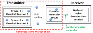
Figure 1: Overview of the communication elements.

The rest of the paper is organised as follows. Sec. II discusses related work. In Sec. III, we present the set up of our molecular communications problem and relevant results from [Awan:2017fm]. Sec. LABEL:sec:pdp:approx present results on input impedance, log-posteriori probability approximation and the design of the enzymatic circuit. We then present simulation results in Sec. LABEL:sec:eval and conclude in Sec. LABEL:sec:con.

II Related Work

There are many surveys on molecular communications, some of these surveys discuss extensively on the use of chemical reactions in molecular communications, e.g., [Bi:CST:2021, Jamali:ProcIEEE:2019, Femminella:DSP:2022]. We have already discussed some existing work [Kuscu:TCom:2019][Bi:TCom:2020][Walter:NatureComm:2023][Heinlein:NanoCom:2023] on designing chemical reaction-based receivers in the introduction. Some other similar work is [Unluturk:2015io, Pierobon:2014gl], [Kuscu:2018iy], [Egan:IEEEAccess:2019]. This paper differs from these earlier papers in two key aspects. First, the earlier work assumed that the demodulation is based on one sample point per symbol; however, this work assumes that demodulation is based on the continuous history of the number of active receptors. We showed in [Chou:2019gf] that demodulation using a continuous history gives a lower BER in comparison. Second, the molecular demodulator considered in earlier work did not use enzymatic cycles. To the best of our knowledge, there is few work work [Awan.2018] [Ratti:Molecules:2022] on considering the use of enzymatic cycles in molecular communication; however, the prior work is focused on channel capacity, rather than the design of enzymatic circuits.

In the molecular communication literature, molecular circuits have been studied for various applications. For example, [MrAlessioMarcone:2017te, Marcone:2018kp] present genetic circuits for parity-check. As another example, [Lombardo:TMBMC:2024, Veletic:TNB:2020] studied molecular circuits for inter-cellular communication and targeted drug delivery, however their analysis is based on deterministic models rather than stochastic models which are used in this paper.

Although most of the work that uses chemical reactions in molecular communication is focused on the receiver side, there is also work that consider reaction-based transmitters and medium. For example, [Deng:2017uw] uses chemical reactions to produce transmission signals for molecular communication, [Arjmandi:TNB:2016] considers a transmitter that uses ion channels, [Farahnak:TCOM:2019] considers the use of chemical reactions in the channel to improve communication performance. There is few work in molecular communications that studies the interaction between multiple reaction-based receivers. An early work is [Chou:2013jd]. A recent work [Vakillipoor:TCOM:2024] models the interaction between multiple absorbing receivers which can be considered to be a special type of chemical reactions.

Synthetic biologists have found that the connection of a downstream molecular component to an upstream molecular circuit can have an adverse effect on the behaviour of the upstream circuit. The review paper [McBride:PIEEE:2019] discusses these adverse effects in the context of molecular communications. The paper [Ratti:Molecules:2022] studies the impact of the inter-connection of enzymatic circuits on mutual information. In this paper, we use time-scale separation to achieve high input impedance to minimise the impact of upstream enzymatic cycles.

III Model and Exact Computation of Posteriori Probabilities

This section presents the set up of the following three components in our molecular communication system: the medium, the transmitter and the front-end of the receiver. Note in particular, the front-end of the receiver is an enzymatic cycle. By using this set up and our earlier work [Awan:2017fm], we present an ODE which describes the evolution of posteriori probability over time. This ODE forms the basis of this paper and our goal is to show how we can realise this ODE by using enzymatic cycles in Sec. LABEL:sec:pdp:approx.

III-A Transmission Medium and Transmitter

The modelling framework of this paper mostly follows our previous work [Chou:2015ga][Chou:gc]. We model the medium as a rectangular prism and divide the medium into voxels. We assume that the transmitter and the receiver each occupies a voxel. Note that it is possible to generalise to the case where a transmitter or receiver consists of multiple voxels, see [Riaz:TCom:2020], but we have not done that to simplify the presentation. Although it may not be physically realistic for the receiver to have a cubic shape, this simplified geometry allows us to focus on the signal processing aspect of the receiver.

We assume the transmitter communicates with the receiver using one type of signalling molecule K, which is depicted as blue circles in Fig. 1. The transmitter uses $S=2$ different symbols indexed by $s=0,1$. (Generalisation to the $S>2$ case is left for further research.) We assume that the transmitter uses concentration shift keying where each symbol $s$ is characterised by a constant mean production rate of signalling molecules and each symbol is produced by a chemical reaction, see Fig. 1. An example of a reaction that can produce molecules at a constant mean rate is:

where $r_{TX}$ denotes the reaction rate constant. In this reaction, signalling molecules are produced at a mean rate of $r_{TX}$ times the concentration of the mRNA molecules. Without loss of generality, in this paper, we assume the transmitter uses (III-A) as the reaction and the transmission symbol $s=0$ (resp. $s$ = 1) is produced by using a lower (higher) mRNA concentration with a common $r_{TX}$ for the two reactions. Note that it is straightforward to generalise the results in this paper to other transmitter reactions as long as they produce the signalling molecule at a mean constant rate. Lastly, we assume that once the signalling molecules have been produced, they are free to diffuse in the medium.

III-B Receiver front-end molecular circuit

The receiver front-end is assumed to be an enzymatic cycle which reacts with the signalling molecule K. The cycle consists of three species X, XK and X_* which take part in the following four reactions:

In order to simplify the presentation here, we will consider a medium consisting of 2 voxels, which we will refer to as Voxel 1 and Voxel 2. (Generalisation to the more general case is straightforward and will be explained later.) We assume that the transmitter and the receiver are located in, respectively, Voxels 1 and 2. The transmitter uses the reaction (III-A) to produce signalling molecules. We assume that when Symbol $s$ is sent, the transmitter uses $m_{s}$ mRNA molecules to produce signalling molecules. As in RDME, the diffusion of the signalling molecules between the voxels is modelled by a unimolecular reaction and we use $\widetilde{d}_{i}$ to denote its reaction rate constant. We also assume that the signalling molecules may leave the medium and we model that as a unimolecular reaction with rate constant $\widetilde{d}_{e}$.

We first show how we can map our Bayesian filtering problem to the one considered in [Bronstein:2018eh], which is based on reaction counts. Let ${\cal R}_{f}(t)$ (resp. ${\cal R}_{r}(t)$) be the cumulative number of times that reaction (LABEL:cr:p:z0:2) (resp. (LABEL:cr:p:z0:3)) has taken place in the time interval $[0,t]$, i.e. ${\cal R}_{f}(t)$ and ${\cal R}_{r}(t)$ are time trajectories of reaction counts. We consider the Bayesian filtering problem which uses ${\cal R}_{f}(t)$ and ${\cal R}_{r}(t)$ as the given information. We argue that we can deduce ${\cal R}_{f}(t)$ and ${\cal R}_{r}(t)$ from ${\cal X}_{*}(t)$. This is because there is only one reaction in which X_* is formed (i.e. reaction (LABEL:cr:p:z0:2)) and only one reaction in which X_* is deactivated (i.e. reaction (LABEL:cr:p:z0:3)); therefore for a given ${\cal X}_{*}(t)$, the corresponding $R_{f}(t)$ and $R_{r}(t)$ can be uniquely determined. Overall, this implies that we can apply the approximation method in [Bronstein:2018eh] to approximate $J_{s}(t)$.

The Bayesian filtering problem is to use the observations ${\cal X}_{*}(t)$ and assumption $s$ to compute the posteriori probabilities of all possible system states that are compatible with the observations. Based on the 2-voxel medium set up which we assume in this appendix, the system state $v(t)$ is the 3-tuple $(K_{1}(t),K_{2}(t),\{XK\}(t))$ where $K_{i}(t)$ is the number of signalling molecules in Voxel $i$ at time $t$. The idea in [Bronstein:2018eh] is to approximate the posteriori probability that the system is in a state by a product of independent Poisson distributions. Let $\theta_{s,1}(t)$, $\theta_{s,2}(t)$ and $\theta_{s,XK}(t)$ denote the means of three independent Poisson distributions in our problem set up. These three Poisson means are used to approximate the posteriori means, as follows: $\theta_{s,i}(t)\approx{\rm E}[K_{i}(t)|s,{\cal X}_{*}(t)]$ ($i=1,2$) and $\theta_{s,XK}(t)\approx{\rm E}[\{XK\}|s,{\cal X}_{*}(t)]$. In particular, $\theta_{s,XK}(t)$ is the approximation that we are seeking. In the following, we will drop the $(t)$ dependence for brevity.

We now present the result of applying the method in [Bronstein:2018eh] to the 2-voxel set up. The result states how the approximate posteriori means $\theta_{s,1}$, $\theta_{s,2}$ and $\theta_{s,XK}$ evolve over time. The evolution of these means consist of both discrete jumps and continuous change. The posteriori mean $\theta_{s,XK}$ experiences a discrete jump at the time when an X_* is formed; at other times, according to [Bronstein:2018eh, Eq. (33)], the evolution of $\theta_{s,i}$ and $\theta_{s,XK}$ obeys the following ODEs:

$$\frac{d\theta_{s,1}}{dt}= r_{TX}m_{s}-(\widetilde{d}_{e}+\widetilde{d}_{i})\theta_{s,1}+\widetilde{d}_{i}\theta_{s,2}$$ (1jnya)

$$\frac{d\theta_{s,2}}{dt}= -(\widetilde{d}_{e}+\widetilde{d}_{i})\theta_{s,2}+\widetilde{d}_{i}\theta_{s,1}-\frac{1}{\Omega}a_{0}\theta_{s,2}\theta_{s,X}$$ (1jnyb)

$$\frac{d\theta_{s,XK}}{dt}= \frac{1}{\Omega}a_{0}\theta_{s,2}\theta_{s,X}-(d_{0}+g_{0})\theta_{s,XK}$$ (1jnyc)

where $\theta_{s,X}=X_{T}-X_{*}(t)-\theta_{s,XK}$ and $X_{T}$ is the total number of substrate molecules in the receiver voxel. This completes the first step which is to apply the method of [Bronstein:2018eh] to our problem.

Our next step is to find an approximation for $\theta_{s,XK}$. Given the history ${\cal X}_{*}(t)$, let $t_{1}$, $t_{2}$, … be time instants that ${\cal X}_{*}(t)$ experiences a jump because an X_* molecule is produced or reverted. In each time interval $(t_{j},t_{j+1})$, the number of X_* molecules is a constant and we denote that by $X_{*,j}$. We note that $\theta_{s,XK}$ in (1jnyc) is a fast variable because $d_{0},g_{0}\gg a_{0}$ so $\theta_{s,XK}$ reaches steady state quickly. Our proposal is to approximate $\theta_{s,XK}$ by a constant value in each time interval $(t_{j},t_{j+1})$ where the constant value is the steady state solution of (1jny) assuming that $X_{*}(t)$ equals to $X_{*}^{[j]}$ for all $t\in[0,\infty)$. Note that our approximation for $\theta_{s,XK}$ is a piecewise constant trajectory over time and the value of the $\theta_{s,XK}$ depends on the value of $X_{*}^{[j]}$ and the kinetic parameters.

Our next step is to determine the steady state solution of (1jny) assuming that $X_{*}(t)$ equals to $X_{*}^{[j]}$ $\forall t\in[0,\infty)$. We will use $\tilde{\theta}_{s,i}$ and $\tilde{\theta}_{s,XK}$ to denote the steady state solution of (1jny). By setting the LHSs of (1jny) to zero, we have, after some manipulations:

$$\left[\begin{array}[]{c}\tilde{\theta}_{s,1}\\ \tilde{\theta}_{s,2}\end{array}\right]= {\underbrace{\left[\begin{array}[]{cc}-(\widetilde{d}_{i}+\widetilde{d}_{e})&\widetilde{d}_{i}\\ \widetilde{d}_{i}&-(\widetilde{d}_{i}+\widetilde{d}_{e})\end{array}\right]}_{\cal D}}^{-1}\;\left[\begin{array}[]{c}-r_{\rm TX}m_{s}\\ g_{1}\tilde{\theta}_{s,XK}\end{array}\right]$$ (1jnaf)

$$\theta_{s,XK}= \frac{1}{\Omega H_{M0}}\tilde{\theta}_{s,2}\;(X_{T}-X_{*}^{[j]}-\tilde{\theta}_{s,XK})$$ (1jnag)

Let $-\alpha_{RX,TX}$ and $-\alpha_{RX,RX}$ be the (2,1) and (2,2) elements of the matrix ${\cal D}^{-1}$. We can re-write the second row of (1jnaf) as:

$$\tilde{\theta}_{s,2}=\alpha_{RX,TX}r_{\rm TX}m_{s}-\alpha_{RX,RX}g_{1}\tilde{\theta}_{s,XK}$$ (1jnah)

The constants $-\alpha_{RX,TX}$ (resp. $-\alpha_{RX,RX}$) quantify the transfer of molecules from the transmitter voxel (receiver voxel) to the receiver voxel. We can identify $\alpha_{RX,TX}r_{\rm TX}m_{s}$ as the steady state mean number of K molecules in the receiver voxel, so we will denote it by $K_{s}^{\rm ss}$ which is the notation that we have used in the main text to denote such as quantity.

By substituting the expression of $\tilde{\theta}_{s,2}$ in (1jnah) into the RHS of (1jnag), we can show that $\tilde{\theta}_{s,XK}$ is the smaller root of the quadratic equation $q_{2}x^{2}+q_{1}x+q_{0}=0$ in the indeterminate $x$ where the coefficients are given by:

$$q_{2}= \alpha_{\rm RX,RX}\frac{g_{1}}{\Omega}$$ (1jnai)

$$q_{1}= -(\alpha_{\rm RX,RX}g_{1}\frac{X_{T}-X_{*}^{[j]}}{\Omega}+\frac{K_{s}^{\rm ss}}{\Omega}+H_{M0})$$ (1jnaj)

$$q_{0}= \frac{K_{s}^{\rm ss}}{\Omega}(X_{T}-X_{*}^{[j]})$$ (1jnak)

Under the condition that $H_{M0}\gg\min(\alpha_{\rm RX,RX}g_{1}\frac{X_{T}}{\Omega},\frac{K_{s}^{\rm ss}}{\Omega})$, we can apply the approximation in [Straube.2017sal] to show that $\tilde{\theta}_{s,XK}\approx-\frac{q_{0}}{q_{1}}$ or

$$\tilde{\theta}_{s,XK}\approx\frac{\frac{K_{s}^{\rm ss}}{\Omega}(X_{T}-X_{*}^{[j]})}{\alpha_{\rm RX,RX}g_{1}\frac{X_{T}-X_{*}^{[j]}}{\Omega}+\frac{K_{s}^{\rm ss}}{\Omega}+H_{M0}}$$ (1jnal)

Since the term $H_{M0}$ in the denominator is much greater than the other two terms, we will replace $X_{*}^{[j]}$ by the steady state mean of $X_{*}(t)$ assuming Symbol $s$ is sent, which we will denote by $\bar{X}_{s}$. This is so that the denominator is independent of the observation $X_{*}^{[j]}$. Furthermore, the RHS of (1jnal) is the expression for the time interval $(t_{j},t_{j+1})$. Since $X_{*}^{[j]}=X_{*}(t)\forall t\in(t_{j},t_{j+1})$, we can therefore obtain a $\tilde{\theta}_{s,XK}$ which holds for all $t$ by replacing $X_{*}^{[j]}$ in the RHS of (1jnal) by $X_{*}(t)$. After that, we obtain (LABEL:eqn:Js:approx) where we have used $\tilde{\theta}_{s,XK}$ as the approximation of $J_{s}(t)$.

Finally, we consider the condition

$$H_{M0}\gg\min(\alpha_{\rm RX,RX}g_{1}\frac{X_{T}}{\Omega},\frac{K_{s}^{\rm ss}}{\Omega})$$ (1jnam)

for the approximation in this Appendix to hold. The quantity $\frac{K_{s}^{\rm ss}}{\Omega}$ is the concentration of the signalling molecules in the receiver voxel when the receiver is absent. We consider this quantity in Sec. LABEL:sec:pdp:approx:front_end:para and denote it by $\bar{[K]}_{s,RX}$. In Sec. LABEL:sec:pdp:approx:front_end:para, we impose the condition $H_{M0}\gg\bar{[K]}_{s,RX}$ so that the front-end molecular circuit has high input impedance. It can be shown that if $H_{M0}\gg\bar{[K]}_{s,RX}$ holds, then (1jnam) holds. Therefore, the condition needed for high impedance is sufficient for the results in this Appendix to hold.

The derivation above assumes that there are only 2 voxels. Therefore, the matrix ${\cal D}$ in (1jnaf) is 2-by-2. If there are $N_{v}$ voxels, then the corresponding ${\cal D}$ is a $N_{v}$-by-$N_{v}$ matrix which models the diffusive movements of the signalling molecules in the medium. In this case, the vector on the RHS of (1jnaf) has 2 non-zero elements situated at the positions corresponding to the transmitter and receiver voxels. By appropriately picking out the elements in ${\cal D}^{-1}$, we will arrive at an equation of the same form as (1jnah). Therefore, even when there are $N_{v}$ voxels, the approximation for $\tilde{\theta}_{s,XK}$ has the same form as (1jnal).

Appendix D Derivation for (LABEL:eqn:pdp:llr:Xstar_only)

The aim of this appendix is to show that the log-probability ratio computation in (LABEL:eqn:ode:L:kappa) can be approximated by (LABEL:eqn:pdp:llr:Xstar_only). We begin by writing (LABEL:eqn:ode:L:kappa) in the integral form:

$$L(T)= \int_{0}^{T}\left[\frac{dX_{*}(t)}{dt}\right]_{+}\log\left(\frac{\kappa_{1}}{\kappa_{0}}\right)dt\;-$$

$$k_{0}\left(\kappa_{1}-\kappa_{0}\right)\int_{0}^{T}(X_{T}-X_{*}(t))dt$$ (1jnan)

The derivation is divided into 2 steps where each step focuses on deriving an approximation for one of the integrals in (1jnan).

Step 1: Approximating the first integral in (1jnan) The first integral on the RHS of (1jnan) can be interpreted as $T$ times the mean production rate of X_* molecules. Over a large $T$, we have:

$$\lim_{T\rightarrow\infty}\frac{1}{T}\int_{0}^{T}\left[\frac{dX_{*}(t)}{dt}\right]_{+}dt= \lim_{T\rightarrow\infty}\frac{1}{T}g_{0}\int_{0}^{T}\{XK\}(t))dt$$ (1jnao)

where the RHS of the above equation models the production of X_* from XK according to Reaction LABEL:cr:p:z0:2. Next, at steady state, the production rate of X_* is balanced by its reversing rate, hence we have:

$$\lim_{T\rightarrow\infty}\frac{1}{T}g_{0}\int_{0}^{T}\{XK\}(t))dt= \lim_{T\rightarrow\infty}\frac{1}{T}\int_{0}^{T}g_{-}X_{*}(t)dt$$ (1jnap)

By combining (1jnao) and (1jnap), we can therefore approximate the first integral on the RHS of (1jnan) by:

$$\int_{0}^{T}\left[\frac{dX_{*}(t)}{dt}\right]_{+}dt\approx \int_{0}^{T}g_{-}X_{*}(t)dt$$ (1jnaq)

Step 2: Approximating the second integral in (1jnan) We now move onto the second integral on the RHS of (1jnan). The derivation here assumes that the system is in steady state, this allows us to replace the time average in by its ensemble average. In this part, we will overload the symbols $X$, $X_{*}$ and $\{XK\}$ to refer to the random variables of the number of, respectively, X, X_* and XK molecules at steady state. This should not cause any confusion because the meaning should be clear from the context. With this overloading, the mean number of X at steady state is denoted by ${\rm E}[X]$ etc. We first need to state or derive a number of auxiliary results.

We first need make a clarification on the notation. The reason we add a pair of curly brackets to the notation $\{XK\}$, which denotes the random variable of the number of XK molecules in steady state, is to stress that it is referring to complex XK. This is important because we will also be multiplying the random variables $X$ and $K$ in the derivation and we will write the multiplication as $X\cdot K$.

We will now derive or present a number of auxiliary results. After that we will combine all these auxiliary results to arrive at an approximation for the second integral in (1jnan).

(Auxiliary Result 1) At steady state, the production and reversion of the XK molecules balance out, therefore, we have:

$$\frac{a_{0}}{\Omega}{\rm E}[X\cdot K]= (d_{0}+g_{0}){\rm E}[\{XK\}]$$ (1jnar)

In terms of ensemble averages, we can rewrite (1jnao) as $g_{0}{\rm E}[\{XK\}]=g_{-}{\rm E}[X_{*}]$. By combining this with (1jnar), we have Auxiliary Result 1:

$${\rm E}[X\cdot K]= \frac{H_{M0}\Omega}{\gamma}{\rm E}[X_{*}]$$ (1jnas)

(Auxiliary Result 2) Since the receiver front-end circuit has high input impedance, it means that we can approximate the signalling molecule count in the receiver voxel when the front-end is present by the one when the receiver is absent, we will therefore ignore the present of the front-end for deriving this auxiliary result. Since the diffusion of the molecules is independent, the distribution of the signalling molecules in the receiver voxel is binomial. We will state a property of the approximation of the reciprocal of the mean of a binomial variable in this auxiliary result.

Consider a binomial distribution $B(Q;m,f)$ with parameters $m$ (number of trials) and $f$ (success probability), then for sufficiently large $m$ and $f$, we have

$$\frac{1}{{\rm E}[Q]}\approx \;{\rm E}[I(\frac{1}{Q})]$$ (1jnat)

where

$$I(\frac{1}{q})= \left\{\begin{array}[]{cl}0&\mbox{for }q=0\\ \frac{1}{q}&\mbox{for }q\geq 1\end{array}\right.$$ (1jnaw)

This result essentially says that the mean of the reciprocal of a binomial random variable (with $\frac{1}{0}$ excluded) is approximately equal to the reciprocal of the mean of the binomial random variable. If $f=1$ and $m\geq 1$, the binomial distribution has a single outcome with a non-zero probability so (1jnaw) is exact. Intuitively, if a probability has a single modal distribution with a narrow spread, then (1jnaw) holds approximately. For $f=0.1$, the relative error of using (1jnaw) is 3.21% for $m=300$ and drops to 1.87% for $m=500$. In general, the approximation is better for large $m$ and $f$.

(Auxiliary Result 3) Since the forward reaction in (LABEL:cr:p:z0:1) is slow because $a_{0}$ is assumed to be small, we can show that:

$${\rm E}[(X_{T}-X_{*})\cdot K]\approx \;{\rm E}[X_{T}-X_{*}]\;{\rm E}[K]$$ (1jnax)

We first write ${\rm E}[X\cdot K]$ as a time integral:

$${\rm E}[X\cdot K]=\int_{t=0}^{\infty}X(t)K(t)dt$$ (1jnay)

The reason why we are considering this integral is because X and K are the reactants of the slow reaction in (LABEL:cr:p:z0:1). This means that the counts of X change slower than that of K. This difference in time-scale allows us to approximate the above integral.

Let $t_{0}$, $t_{1}$, $\ldots$ be a sequence of time instants at which $X(t)$ changes its value. We will re-write the integral on the RHS of (1jnay) as a sum of integrals:

$$\int_{t=0}^{\infty}X(t)K(t)dt= \sum_{i=0}^{\infty}X(t_{i})\int_{t_{i}}^{t_{i+1}}K(t)\;dt$$ (1jnaz)

Since $X(t)$ is slow in comparison with $K(t)$, this means the time interval $[t_{i},t_{i+1})$ is likely to be long compared to the time-scale of the faster $K(t)$. This allows us to approximate the integral on the RHS of (1jnaz) by ${\rm E}[K](t_{i+1}-t_{i})$. Hence we have:

$${\rm E}[X\cdot K]= \sum_{i=0}^{\infty}X(t_{i})E[K]\;dt$$

$$= {\rm E}[X]\;{\rm E}[K]$$ (1jnba)

Note that the above argument is identical to the one used in [Cao:2005gj] to derive the slow-scale tau-leaping simulation algorithm.

Next, we do two substitutions. First, we note that Auxiliary Result 1 expresses ${\rm E}[X\cdot K]$ in terms of ${\rm E}[X_{*}]$. Second, we approximate ${\rm E}[X]$ by ${\rm E}[X_{T}-X_{*}]$ because we know the front-end circuit has high input impedance so ${\rm E}[\{XK\}]$ is small. After these substitutions, we arrive at Auxiliary Result 3:

$${\rm E}[X_{T}-X_{*}]\approx\;\frac{H_{M0}\Omega}{\gamma}\frac{{\rm E}[E_{*}]}{{\rm E}[K]}$$ (1jnbb)

(Auxiliary Result 4) By using the same argument as in Auxiliary Result 3, we can show that:

$${\rm E}[X_{*}I(\frac{1}{K})]\approx \;{\rm E}[X_{*}]\;{\rm E}[I(\frac{1}{K})]$$ (1jnbc)

By using the above auxiliary results we have

$${\rm E}[X_{T}-X_{*}]$$

$$\approx \frac{H_{M0}\Omega}{\gamma}\frac{{\rm E}[E_{*}]}{{\rm E}[K]}\;\;$$ (Aux. Result 3)

$$= \frac{H_{M0}\Omega}{\gamma}{\rm E}[E_{*}]{\rm E}[I(\frac{1}{K})]\;\;$$ (Aux. Result 2)

$$= \frac{H_{M0}\Omega}{\gamma}{\rm E}[X_{*}I(\frac{1}{K})]\;\;$$ (Aux. Result 4) (1jnbd)

By applying the results in the 2 steps above, we can show that (LABEL:eqn:ode:L:kappa) can be approximated by:

$$\frac{L(t)}{dt}= g_{-}X_{*}(t)\left[\log\left(\frac{\kappa_{1}}{\kappa_{0}}\right)-H_{M0}\Omega\frac{\kappa_{1}-\kappa_{0}}{K(t)}\right]$$ (1jnbe)

which is (LABEL:eqn:pdp:llr:Xstar_only).

Appendix E Deriving (LABEL:eqn:pdp:hyperbolic)

In this Appendix, we will show that the enzymatic circuit (LABEL:cr:p:Z1:all), which is referred to as the threshold-hyperbolic (TH) circuit in Sec. LABEL:sec:Lhat:TH, can be used to realise a TH function. Since the TH-cycle has multiple non-linearities, a stochastic analysis is not tractable. Instead, we will use quasi-steady state analysis [Gomez-Uribe:PLoS_CB:2005] which is also used in Appendix LABEL:app:front_end. We further simplify the analysis by not including the diffusion of K in the model. We justify this simplification by the fact that we will require the TH-cycle to have high input impedance which means few K molecules will be sequestered by this circuit. This in turn means that the behaviour of the TF-circuit can be analyse without considering the details on diffusion. Based on these simplifications, we assume that the total count of K molecules seen by the circuit is a constant and we will denote this by $K_{T}$ where $K_{T}$ can be considered to be the mean steady state count of signalling molecules in the receiver voxel. We expect $K_{T}=[K]_{s}^{\rm ss}\Omega$.

We will show that under the assumptions that $H_{M1}\gg\frac{K_{T}}{\Omega}$, $H_{M2}\ll\frac{P_{T}}{\Omega}$ and $\frac{k_{1}K_{T}}{k_{2}P_{T}}$ is sufficiently large, then the amount of Y_* in the TH-cycle is a threshold-hyperbolic function of $K_{T}$ which is the input level of the circuit.

Our derivation makes use of the results in [Straube.2017sal] which uses quasi-steady analysis to study the properties of enzymatic cycles of the form (LABEL:cr:p:Z1:all). Since the quasi-steady state analysis uses concentration rather than counts, we will temporarily switch over to concentration so that the reader can better match the formulas here with those in [Straube.2017sal]. Note that all the concentrations in this Appendix are steady state concentrations.

The implication of the assumption $H_{M2}\ll[P]_{T}$ has been studied in [Straube.2017sal]. Let ${\cal Y}=[Y_{*}]+[Y_{*}P]$. By using [Straube.2017sal, Eq. (29)], which holds when $H_{M2}\ll[P]_{T}$, we have:

$$[Y_{*}P] \approx \left\{\begin{array}[]{ll}{\cal Y}\left(1-\frac{H_{M2}}{[P]_{T}-{\cal Y}}\right)&\mbox{ for }{\cal Y}<[P]_{T}\\ [P]_{T}\left(1-\frac{H_{M2}}{{\cal Y}-[P]_{T}}\right)&\mbox{ for }{\cal Y}>[P]_{T}\end{array}\right.$$ (1jnbh)

Since we assume $H_{M2}$ is small, we set $H_{M2}$ to zero in the above expressions. After some simplification, we have:

$$[Y_{*}] \approx 0 \mbox{ for }[Y_{*}]+[Y_{*}P]<[P]_{T}$$ (1jnbi)

$$[Y_{*}P] \approx[P]_{T} \mbox{ for }[Y_{*}]+[Y_{*}P]>[P]_{T}$$ (1jnbj)

Note that $[Y_{*}]+[Y_{*}P]$ is small when the input level is small, and vice versa. This derivation shows that if the input level is low, then according to (1jnbi) we have $[Y_{*}]\approx 0$ or few Y_*. This is the threshold part of the threshold-hyperbolic function. On the other hand, if the input level is high, then according to (1jnbj), we have $[Y_{*}P]\approx[P]_{T}$ or P is saturated.

We now focus on deriving an expression for $[Y_{*}]$ when the input is high. The assumption $H_{M1}\gg\left(1+\frac{k_{1}}{k_{2}}\right)K_{T}$ implies that the following holds [Straube.2017sal, Eq. (67)]:

$$[Y_{*}]+[Y_{*}P]$$

$$= [Y]_{T}-\frac{[K]_{T}+H_{M1}}{\alpha-1}\mbox{ for }[Y_{*}]+[Y_{*}P]>[P]_{T}$$ (1jnbk)

where $\alpha=\frac{k_{1}[K]_{T}}{k_{2}[P]_{T}}$. By suitable choice of the enzymatic cycle parameters, we can make $\alpha>1$ and recall that $[Y_{*}P]\approx[P]_{T}$, therefore we have:

$$[Y_{*}] = \widetilde{h}_{0}-\frac{\widetilde{h}_{1}}{[K]_{T}}$$ (1jnbl)

where $\widetilde{h}_{0}=[Y]_{T}-[P]_{T}-\frac{k_{2}}{k_{1}}[P]_{T}$ and $\widetilde{h}_{1}=\frac{k_{2}}{k_{1}}[P]_{T}H_{M1}$. This shows that the concentration of Y_* (i.e., $[Y_{*}]$) is a hyperbolic function of the input level $[K]_{T}$ when the input is high. The result (1jnbl) is expressed in concentration, by multiplying its both sides by $\Omega$, we obtain (LABEL:eqn:pdp:hyperbolic).

Appendix F Parameters for the TH-cycle

This appendix explains how we determine the rate constants of the TH-cycle (LABEL:cr:p:Z1:all) to realise the scaled TH function:

$$\left[\underbrace{\rho\log\left(\frac{\kappa_{1}}{\kappa_{0}}\right)}_{\zeta_{0}}\;-\;\underbrace{\rho H_{M0}(\kappa_{1}-\kappa_{0})}_{\zeta_{1}}\;\frac{\Omega}{K_{T}}\right]_{+}$$ (1jnbm)

where $\rho>0$ is a scaling constant. The value of $\rho$ can be chosen so that the probability that Y is active is high when the number of K molecules is high. Note that if one scales the log-probability ratio (LABEL:eqn:pdp:llr_approx) and the detection decision threshold by the same constant, the property of the detector does not change, therefore the scaling mentioned above is allowed.

We assume that $\rho$ has been chosen beforehand, so we can assume $\zeta_{0}$ and $\zeta_{1}$ are given. In addition, as stated in Sec. LABEL:sec:Lhat:X_times_Y, we use molecules of the form X-Y to realise the computation of on the RHS of (LABEL:eqn:pdp:llr_approx). This means that $[X]_{T}=[Y]_{T}$. Here, we assume that the concentration $[X]_{T}$ has been chosen and that means the concentration $[Y]_{T}$ has been fixed.

By comparing (1jnbm) and (1jnbl), we have:

$$[Y]_{T}-[P]_{T}-\frac{k_{2}}{k_{1}}[P]_{T} = \zeta_{0}$$ (1jnbn)

$$\frac{k_{2}}{k_{1}}[P]_{T}H_{M1} = \zeta_{1}$$ (1jnbo)

The Michaelis-Menten constant $H_{M1}$ needs to be much bigger than $[K]_{T}$ for the cycle (LABEL:cr:p:Z1:all) to behave as a threshold-hyperbolic function. We arbitrarily choose $H_{M1}$ to be 10 times larger than the maximum $[K]_{T}$ that the PH-cycle will encounter which happens when Symbol 1 is sent. Once $H_{M1}$ has been fixed, the values of $\frac{k_{1}}{k_{2}}$ and $[P]_{T}$ can be solved from the above two equations for the given $[Y]_{T}$.

Since we need $[P]_{T}\gg H_{M2}$ for the threshold-hyperbolic behaviour, we set $H_{M2}=\frac{[P]_{T}}{80}$ where 80 is an arbitrary choice. As mentioned in Sec. LABEL:sec:Lhat:X_times_Y, we choose $k_{1}$ and $k_{2}$ so that the reaction time-scales of X and Y are similar. However, note that we have determined the ratio $\frac{k_{1}}{k_{2}}$ earlier so the choice of $k_{1}$ and $k_{2}$ need to satisfy this ratio. Finally, for the other reaction rate constants, we make an arbitrary choice of $d_{1}=k_{1}$ and $d_{2}=k_{2}$, then $a_{1}$ and $a_{2}$ are computed from the definitions of $H_{M1}$ and $H_{M2}$.

Appendix G RHS of (LABEL:eqn:pdp:llr_approx) is proportional to the number X_*-Y_* molecules

The aim of this appendix is to show that, at steady state, the RHS of (LABEL:eqn:pdp:llr_approx) is proportional to the number X_*-Y_* molecules. An assumption that we need in our proof is that the activations of X and Y by K are independent, i.e., we have:

$${\rm P}[\mbox{\ce{X-Y} in state \ce{X_*-Y_*}}]$$

$$= {\rm P}[\mbox{\ce{X} site in \ce{X-Y} is in \ce{X_*} state}]\times$$

$${\rm P}[\mbox{\ce{Y} site in \ce{X-Y} is in \ce{Y_*} state}]$$ (1jnbp)

Let $\{X-Y\}_{T}$ be the total number of X-Y molecules in its various states. Also, let $\{X_{*}-Y_{*}\}^{\rm ss}$ be the steady state number of molecules in the X_*-Y_* state, $X_{*}^{\rm ss}$ (resp. $Y_{*}^{ss}$) is steady state number of molecules where the X (Y) site in the X_* (Y_*) state. We can rewrite (1jnbp) as:

$$\frac{\{X_{*}-Y_{*}\}^{\rm ss}}{\{X-Y\}_{T}}=\frac{X_{*}^{\rm ss}}{\{X-Y\}_{T}}\times\frac{Y_{*}^{\rm ss}}{\{X-Y\}_{T}}$$ (1jnbq)

We now start with the RHS of (LABEL:eqn:pdp:llr_approx) at steady state, which is proportional to the product of $X_{*}^{\rm ss}$ and that of the TH-function. Since we show in Appendix E that the TH-function is proportional to $Y_{*}^{ss}$, therefore, the RHS of (LABEL:eqn:pdp:llr_approx) is proportional to the product $X_{*}^{\rm ss}Y_{*}^{\rm ss}$. By (1jnbq), we can therefore conclude that the RHS of (LABEL:eqn:pdp:llr_approx) at steady state is proportional to the number of molecules in the X_*-Y_* state.

Appendix H Parameters of the transmitter and enzymatic cycles

For the transmitter, $r_{\rm TX}=3.38$ s^-1 in Reaction (III-A). For TX-setting-1, Symbols 0 and 1 are generated by using, respectively, 96 and 320 mRNA molecules. For TX-setting-2, these numbers are changed to 32 and 96 mRNA molecules.

The parameters of the cycle (LABEL:cr:p:Z1:all) are: $a_{1}$ = 0.0463; $d_{1}$ = 250; $k_{1}$ = 250; $a_{2}$ = 24.24; $d_{2}$ = 39.24; $k_{2}$ = 39.24; and, $P_{T}$ = 10.

The parameters of the cycle (LABEL:cr:p:int:all) are: $a_{3}$ = 2$\times 10^{-4}$; $d_{3}$ = 100; $k_{3}$ = 100; $a_{4}$ = 2$\times 10^{-6}$; $d_{4}$ = 1; $k_{4}$ = 1; $J_{T}$ = 185; and, $\tilde{P}_{T}$ = 30.