The Milky Way Atlas for Linear Filaments

Abstract

Context. Filamentary structure is important for the ISM and star formation. Galactic distribution of filaments may regulate the star formation rate in the Milky Way. However, interstellar filaments are intrinsically complex, making it difficult to study quantitatively.

Aims. Here, we focus on linear filaments, the simplest morphology that can be treated as building blocks of any filamentary structure.

Methods. We present the first catalog of 42 “straight-line” filaments across the full Galactic plane, identified by clustering of far-IR Herschel HiGAL clumps in position-position-velocity space. We use molecular line cubes to investigate the dynamics along the filaments; compare the filaments with Galactic spiral arms; and compare ambient magnetic fields with the filaments’ orientation.

Results. The selected filaments show extreme linearity ($>$10), aspect ratio (7-48), and velocity coherence over a length of 3-40 pc (mostly $>$10 pc). About 1/3 of them are associated with spiral arms, but only one is located in arm center, a.k.a. “bones” of the Milky Way. A few of them extend perpendicular to the Galactic plane, and none is located in the Central Molecular Zone (CMZ) near the Galactic center. Along the filaments, prevalent periodic oscillation (both in velocity and density) is consistent with gas flows channeled by the filaments and feeding the clumps which harbor diverse star formation activities. No correlation is found between the filament orientations with Planck measured global magnetic field lines.

Conclusions. This work highlights some of the fundamental properties of molecular filaments and provides a golden sample for follow-up studies on star formation, ISM structure, and Milky Way structure.

1 Introduction

Filamentary structure is the dominant morphology of the interstellar medium (ISM), and molecular filaments can play an important role in star formation (Hacar et al., 2023). The Galactic distribution of filaments may regulate the global star formation rate in the Milky Way. The largest filaments can map out the skeleton (“bones”) of the Milky Way in spiral arms (Wang et al., 2015; Zucker et al., 2015; Vallée, 2016). However, the inherent complexity and hierarchy of molecular filaments make it challenging to characterize the structure and dynamics important for star formation. Traditionally, to study star formation, maps of molecular clouds are often decomposed into cores (e.g. Williams et al., 1994; Berry, 2015), and in recent years, also to filaments (e.g. Men’shchikov, 2013; Koch & Rosolowsky, 2015).While spherical cores, by definition, are simple in morphology and thus are relatively easy to treat theoretically, filaments are not. More critically, the community has not yet reached a consensus on the definition of what is a filament, resulting a wide range of “filaments” reported in the literature, from simple filaments of linear L-shape, C-shape, S-shape filaments, to a network of filamentary structure of X-shape (Wang et al., 2015), and Hub-Filament Systems (Myers, 2010). A meaningful comparison amongst those filaments are thus difficult, because they are intrinsically different entities (c.f. Zucker et al., 2018).

We proposed a physically driven definition of filaments (Wang et al., 2016) inspired by the “sausage instability” of a gaseous cylinder (Chandrasekhar & Fermi, 1953). Under self-gravity, a supercritical filament radially collapse and fragments into a string of equally-spaced clumps. Built on this picture, we developed a customized minimum spanning tree (MST) algorithm to identify filaments by clustering clumps in position-position-velocity (PPV) space. We applied this to PPV clump catalogs decomposed from three Galactic plane surveys: BGPS, ATLASGAL, and SEDIGISM (Wang et al., 2016; Ge & Wang, 2022; Ge et al., 2023, hereafter Paper I, II, III). However, those surveys cover only a portion of the Galactic plane. More importantly, those filaments and others reported in the literature so far have a large variety of linearity and morphology classes. Such limitations prevent a further characterization of the fundamental common properties of filaments. A full Galactic plane census of the “same entities” is highly demanded.

Here, we identify and characterize the most collimated, “straight-line” like filaments across the full Galactic plane, using data from the Herschel HiGAL survey. Among all the morphology types (Wang et al., 2015), linear filaments are the simplest, and can be treated as “unit” filaments, or building blocks of more complicate filamentary structures. Physical characterization of these units can pave the way towards a unified understanding of filaments (Liu et al., 2018; Zucker et al., 2018). For example, how long can a straight-line filament extend in our Galaxy? How do they distribute in the Galaxy and map out the spiral arms? What role do they play in star formation? Answer to these questions are crucial for a quantitative understanding of star formation in our and other galaxies, as interferometric observations are routinely resolving the largest filaments in nearby galaxies (Wang et al., 2015). This work provides a key step forward.

(a)
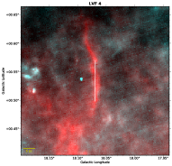
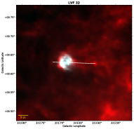
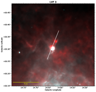
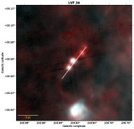
(b)
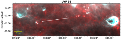
(c)

Figure 1: (a) Representative filaments in a two-color view, where Herschel 250 $\mu\mathrm{m}$ and 70 $\mu\mathrm{m}$ emission are shown in red and cyan, respectively. A filament is marked by end-to-end line connecting two clumps at the filament tips. From left to right are four representative categorizes: “Quiescent”, “Flower”, “Central”, and “Necklace”. Figure 3 show all filaments. (b) same two-color view but for F36, part of “Nessie”. (c) ¹³CO(2–1) PV plot of F36 along curved filament length, and fitting to the global velocity gradient (red line), where the error bars correspond to $1\sigma$ dispersion. The periodogram of the PV curve after removing the global velocity gradient shows a period at 2 pc, consistent to clump separation (§3.3).

2 Data and Method

The Herschel infrared Galactic Plane Survey (HiGAL) mapped the entire Galactic plane at five bands: 70, 160, 250, 350, and 500 $\mu\mathrm{m}$ (Molinari et al., 2010, 2016). A band-merged catalog has been released, containing a total of $\sim$150k sources with physical properties determined for most sources (Elia et al., 2017, 2021). Of the $\sim$150k sources, $\sim$126k sources have radial velocity resolved using literature data. These sources form by far the deepest, largest, and uniform PPV catalog of dust clumps across the entire Galactic plane, excellent for finding filaments using our MST method. Note that Elia et al. (2021) assigned HiGAL clumps into “high-relaible” and “low-reliable” catalogs based on the quality of SED fitting. Here we merged both catalogs as we are most interested in PPV information to begin with. The HiGAL sources have an average diameter of $25^{\prime\prime}$ and 0.6 pc. For simplicity, we refer them as “clumps” in this paper, although their physical scales can be up to few parsec for sources at large distances.

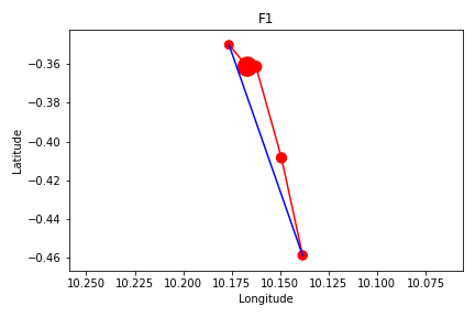
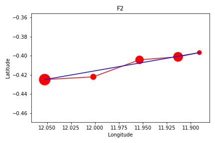
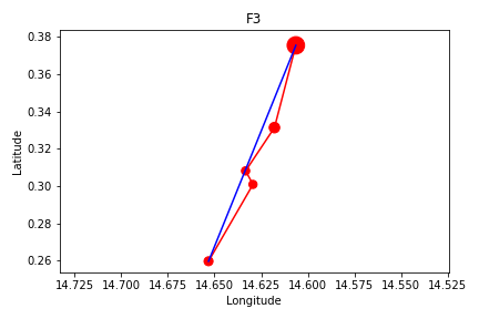
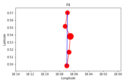
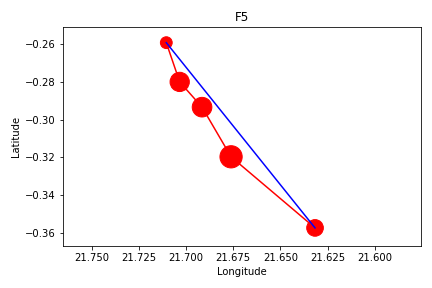
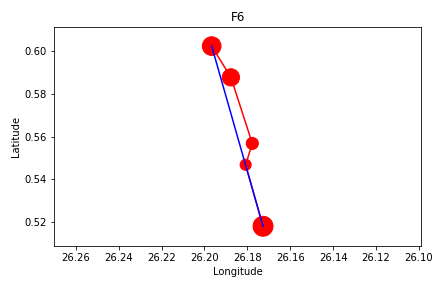
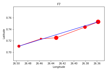
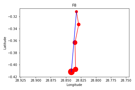
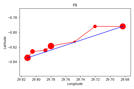
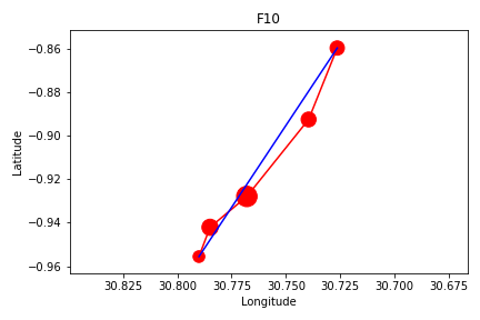
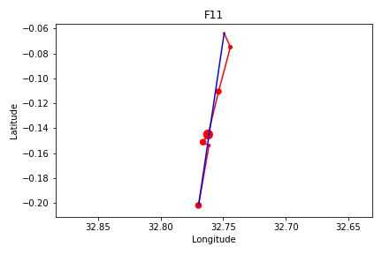
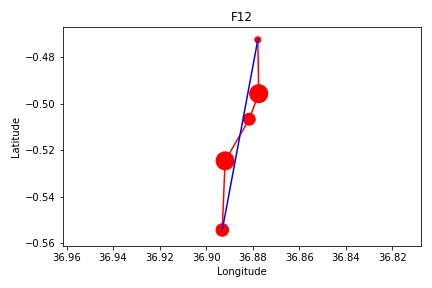
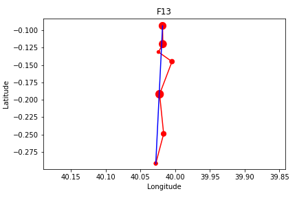
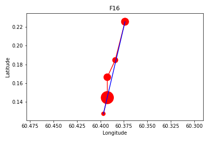
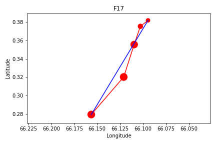
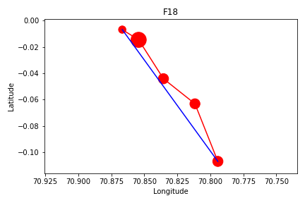
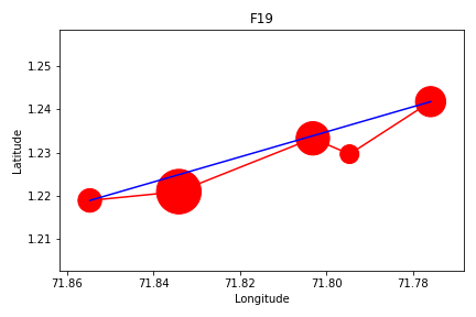
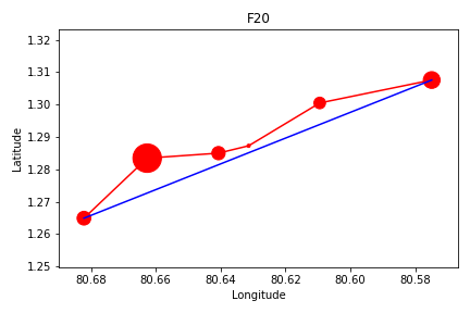
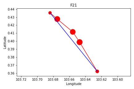
Figure 5: MST for F1 to F21. The red circles represent the position and size of the Herschel/HiGAL clumps, and the red segments are the MST edges connecting the clumps. The blue line marks the filament end-to-end.

We search for filaments using the MST method following Paper I, II, III. In brief, any two clumps in the Elia et al. (2021) catalog are connected only if they are close enough both in position (spatial separation $\Delta s<0.06^{\circ}$) and velocity ($\Delta v<2$ km s^-1). These criteria are resulted from robust tests (details are given in Paper I, II, III). This results to $\sim$3.4k MST “trees” containing at least five clumps. A strict linearity of $>$10 is applied to select the most prominent straight-line filaments. Linearity is defined as the ratio between the spread of clumps along the long and short axes (Paper I, II, Figure 5). The selection results in 42 linear and velocity-coherent (LV) filaments.Most of them are new identification, and only six of them are associated with previously known filaments (Table 1). For example, F36 and F7 are the central and linear part of the well kown S-shaped “Nessie” filament (Jackson et al., 2010; Wang et al., 2015), and the X-shaped Herschel cold filament CFG26 (Wang et al., 2015).

Thanks to HiGAL’s full coverage of the Galactic plane, and the $>$10 times larger number of PPV clumps compared to previous PPV catalogs used in Paper I, II, III, we are able to extract an atlas of linear filaments in the Milky Way’s disk. Unlike in Paper I, II, III, we do not put a length cut ($>$10 pc for large-scale filaments) but strictly limit the linearity to select straight-line filaments. They are the building blocks of more complex filamentary structure, and it is of great interest to investigate their properties.

After finding the filaments (as strings of clumps), we use properties of the HiGAL clumps (Elia et al., 2021) as basis to characterize the filaments (§3.1, 3.5). These include clump position, velocity, distance, diameter, mass, luminosity, temperature, association with 70 $\mu\mathrm{m}$ point source, and evolutionary stages (starless, prestellar, and protostellar). A Galactic spiral arm model is compared to the filaments (§3.2). Molecular line maps are retrieved from public surveys to analyze the dynamics (§3.3, 3.4). Dust polarization maps from the Planck are used to derive global magnetic fields of the filaments (§3.6).

Note that our MST approach is different than other automated identification that directly decompose continuum images (e.g. Schisano et al., 2020; Li et al., 2016), which resulted orders of magnitude more filaments, and did not use velocity information in identification. Our approach uses a uniform PPV catalog as input, and can have a physically driven criteria for filaments. In comparison, Li et al. (2016) identified 517 ATLASGAL filaments merely in the inner Galactic plane; only three have overlaps with our filaments (Table 1). Schisano et al. (2020) identified 32059 candidate filaments using HiGAL images. Generally, those are not the same kind of features as our filaments.

3 Results and Discussion

3.1 Global Properties

Figure 1(a,b) present example filaments in far-IR. Herschel 250 $\mu\mathrm{m}$ emission in red provides a rough proxy for column density, and the 70 $\mu\mathrm{m}$ emission in cyan highlights point sources of embedded young stellar objects, indicative of star formation. The white lines outline the filaments end to end. The 42 filaments can be divided into four categories of star formation activities: “Quiet” (no 70 $\mu\mathrm{m}$ point source), “Flower” (star formation developed at one tip, or head-tail), “Central” (star formation developed in central clumps), and “Necklace” (star formation developed in almost all clumps). Evolution and dynamic effects, including edge collapse (Yuan et al., 2020; Bhadari et al., 2022) likely play a role in shaping the appearance of the filaments, which deserve further study.

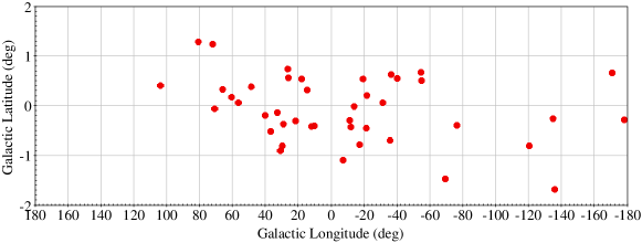
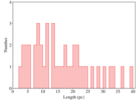
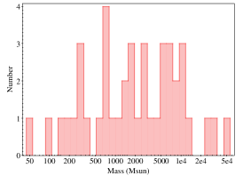
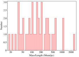
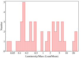
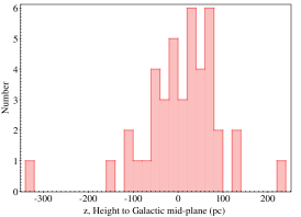
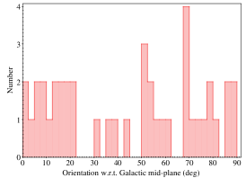
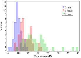
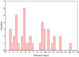
Figure 4: Properties of the 42 linear filaments. Note that some parameters are plotted in log scale for better illustration at the long tails in distribution. The temperature histogram shows the minimum, maximum, and mean temperature of the clumps in filaments. Mass, mass/length ratio, and luminosity are lower limits (§3.1).

Table 1 lists physical properties of the filaments, and Figure 4 illustrates the distribution of some parameters.

Distance is determined from the distances of the clumps in a filament. For most filaments, the clumps have consistent distances reported in Elia et al. (2021). Only in few cases (F1, 9, 39, 41, 42), the clump distances are spread and containing near and far distances. In those cases, additional judgements are made based on the infrared extinction/emission to adopt either near or far distance for the filaments. Clumps in three filaments (F13, 22, 30) have no available distance; we compute distances using the parallax-based Bayesian distance estimator provided by (Reid et al., 2019, 2016).

No obvious selection effect is seen in the distance histogram (Figure 4), which shows a broad range from 1.2-16.3 kpc, and a weak peak at 4-5 kpc, corresponding to the “Galactic molecular ring” (Jackson et al., 2006). After determining the filament distance, related clump parameters in Elia et al. (2021) are scaled accordingly to computer filament properties.

Originated from selection, the filaments show remarkable linearity and aspect ratios. Filament length is measured by the sum of the MST edges (thus following the curvature), and adding sizes of the two edge clumps to account for the actual length of the filament. This “edge length” is on average only 3% (and up to 12%) larger than the “end-to-end length” by simply connecting the two clumps at the tips with a straight line (shown in Figure 1). The small curvature provides another measure of the extreme linearity resulted from the selection criteria. Of the 42 filaments, 28 are longer than 10 pc, satisfying the “large-scale” filaments in Paper I, II, III. The aspect ratios (7-48) are among the highest reported in the literature.

A lower limit of filament mass ($5\times 10^{1}$ to $5\times 10^{4}$ $M_{\odot}$) is given by the sum of clump masses. According to Paper II, this lower limit is typically 36% of the total filament mass.

A global velocity gradient is determined by a linear fit to the ($l_{i},v_{i}$) plot, where $l_{i}$ is the length along filament, and $v_{i}$ the LSR velocity of the $i$th clump in a filament. Note that the slope (velocity gradient) of the fitted lines can be positive or negative, depending on the orientation.

Mass, luminosity, and luminosity-to-mass ratio are among the sharpest distributions (Kurtosis $K=12,22.5,8$, Table 1). But those are dominated by a long tail at the right side made of only three large values. If those outliers are removed, the distributions would be quite flat. Aspect ratio, number of clumps, and angular length also show sharp distributions ($K=7.5,10,10$) with no obvious outliers.

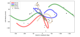
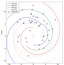
Figure 2: Galactic distribution of the 42 linear filaments compared with spiral arms of the Taylor & Cordes (1993) model, with a width of 10 km s^-1. Upper panel shows the Galactic longitude vs. LSR velocity, and the bottom panel shows a “face-on” view of the Milky Way, where the Sun ($\odot$) and the Galactic center ($+$) are marked. The dashed circle marks the solar circle that separates inner and outer Galaxy.

3.2 Galactic Distribution and Association with Spiral Arms

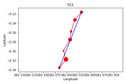
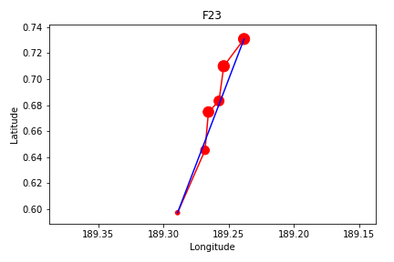
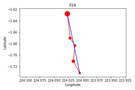
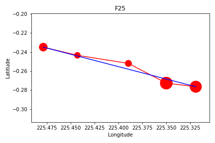
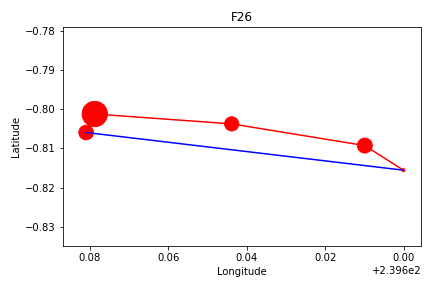
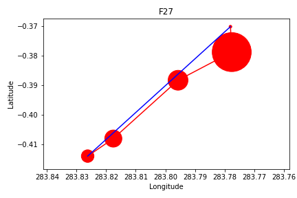
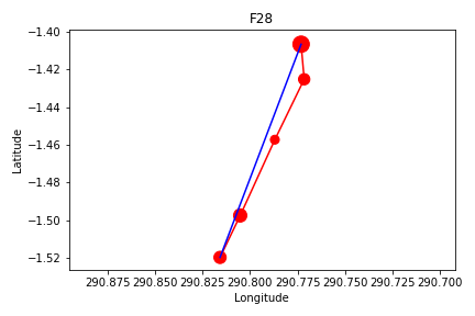
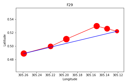
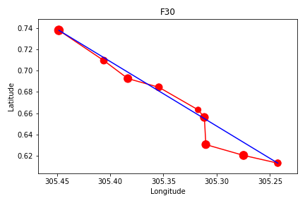
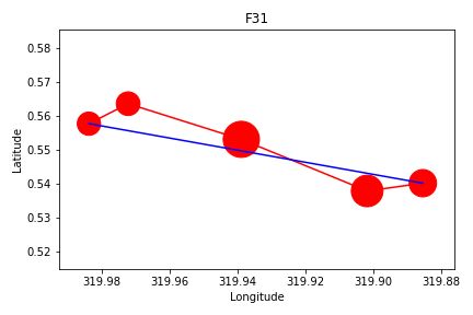
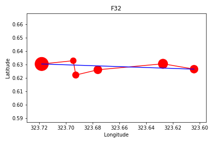
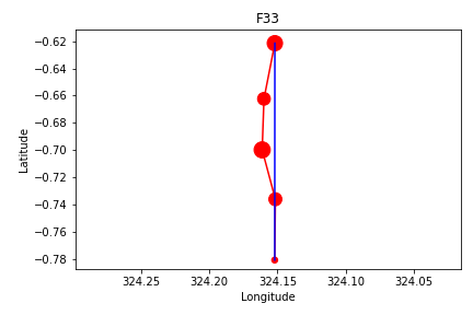
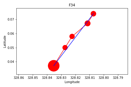
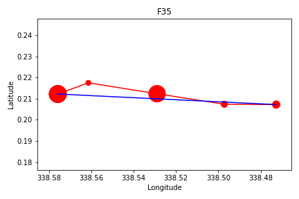
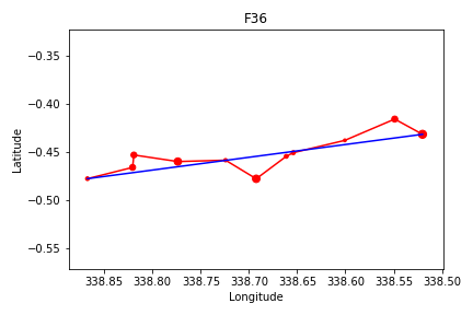
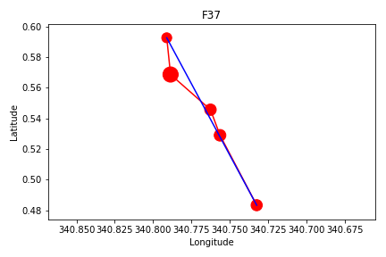
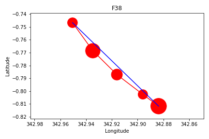
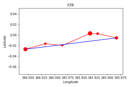
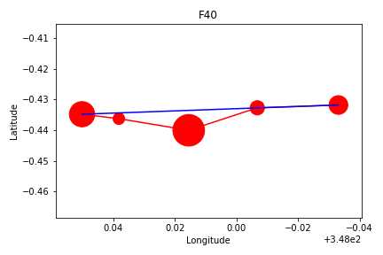
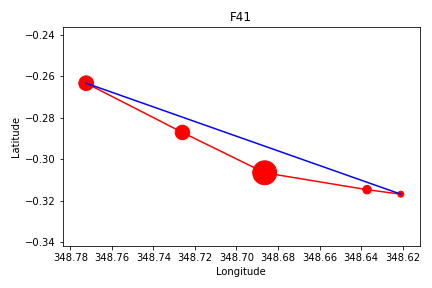
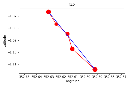
Figure 2: Continued. MST for F22 to F42.

The 42 linear filaments are located in all the four Galactic quadrants, concentrating in the I (20 filaments) and IV (16 filaments) quadrants, while the II and III quadrants have only 2 and 5 filaments, respectively (Figure 4, Figure 2). Interestingly, no linear filaments are found near the Galactic center, in the Central Molecular Zone (CMZ, Lu et al., 2019), and at low longitudes of $-8^{\circ}<l<10^{\circ}$. The averaged Galactic longitude and latitude of the filaments are $(l,b)=(-8.92,-0.05)$ deg. Distributions of both $l$ and $b$ slightly skew towards negative side (Skewness $S_{l}=-0.9,S_{b}=-0.2$). The $l$ distribution is slightly more centrally peaked than normal distribution, and the $b$ is flatter ($K_{l}=0.5,K_{b}=-0.1$). After taking distance into account, most filaments are found within the solar circle, with 31 in the inner Galaxy and 11 in the outer Galaxy (Figure 2).

Figure 4 shows that the filaments are concentrated on the Galactic mid-plane ($K_{z}=4.1$), most of which are within height $|z|<100$ pc; only 7 of them are located at a larger height up to 320 pc. In contrast, the orientation of the filaments with respect to Galactic mid-plane ($\theta$) do not show obvious preference ($K_{\theta}=-1.5,S_{\theta}=0$), i.e., these well-defined filaments appear to be randomly orientated (c.f. bimodal distribution in Ge et al., 2024). Notably, a few filaments extend perpendicular to the Galactic plane (e.g., F4 in Figure 1). These properties are important to further understanding the formation of these filaments (e.g. Feng et al., 2024; Zucker et al., 2019).

We compare the filaments to spiral arms following the criteria of Paper I, II, III. We adopt the Taylor & Cordes (1993) spiral arm model, because it is derived based on measurements in all the four Galactic quadrants. More recent models do not have sufficient observations in the southern sky (Paper III). A filament is considered to be associated with a spiral arm when its LSR velocity is within $\pm$5 km s^-1 from the spiral arms in the Galactic longitude-velocity tracks (Figure 2). This results 14 filaments associated with arms: 5 on Perseus, 4 on Sagittarius-Carina, 3 on Scutum-Centaurus, and 2 on Norma-Outer arm. We note that these 14 on-arm filaments have rather spread orientation angles (similar to the entire sample), with only 5 filaments having $\theta\leq 30^{\circ}$, i.e., running almost parallel to the mid-plane (after projection). Surprisingly, among these, only one (F36, central part of Nessie) fulfills additional criterion for a Galactic “bone”, i.e., lying in the center of mid-plane ($|z|\leq 20$ pc). Another 4 “parallel filaments” are offset higher to the mid-plane ($|z|=27-50$ pc).

3.3 Velocity Oscillation along Filaments

Our sample of filaments represent a string of clumps semi equally spaced along the filaments. This “necklace” configuration is a natural result of the “sausage instability” (Chandrasekhar & Fermi, 1953; Ostriker, 1964; Fiege & Pudritz, 2000). Once this configuration is formed, materials can flow along the filaments to feed the clumps, enhancing star formation activities therein. Indeed, fluctuation of velocity along filaments have been observed, consistent with mass flows (Hacar & Tafalla, 2011; Zhang et al., 2015; Wang, 2018; Henshaw et al., 2020).

Our unbiased sample provides an ideal test bed to investigate whether mass flows are common in filaments, and further revealing their properties. Of the 42 filaments, we are able to retrieve molecular line cubes for 20 filaments from public surveys (Jackson et al., 2006; Barnes et al., 2015; Umemoto et al., 2017; Schuller et al., 2017, 2021; Cubuk et al., 2023). These provide ¹³CO(1-0), ¹²CO(1-0), or ¹³CO(2-1) cubes that well resolve the filaments. Few other filaments are also covered by the surveys, but the data quality are insufficient for our following analysis. A position-velocity (PV) cut is extracted along the filaments by connecting the clumps. At a given position along the filament, the intensity weighted centroid velocity (moment 1) and dispersion (moment 2) are plotted in Figure 1(c).

All the 20 PV curves show some variation in velocity along the filaments, most of which appear to be semi-periodic. We first fit a global slope in the PV curve, and then perform periodicity analysis on the residual PV curve, following Wang (2018). For 19/20 filaments, the periodicity analysis reveals one or two dominant periods ($P_{\rm v}$). (The only exception is F12 with a weak peak of $\sim$4 pc period.) In 11 filaments, the primary period match well with $P_{\rm cl}$, defined as the mean separation between the clumps. In the rest of 8 filaments, the secondary period match well with $P_{\rm cl}$. So, in all but one cases, the PV curves are oscillating with either a primary or secondary period that match well with $P_{\rm cl}$. The averaged ratio $P_{\rm v}/P_{\rm cl}$ is $1.0\pm 0.2$. This is in striking consistent with the model proposed by Hacar & Tafalla (2011), and strongly suggest that gas flows are channelled by these linear filaments, and are feeding the clumps. Each of the clumps are potential or ongoing sites for star or star cluster formation (§3.5). The global PV slope may represent net bulk gas motions from end to end of the filament, at a fitted rate of 0.0-0.35 km s^-1/pc (average 0.09 km s^-1/pc). Localized to the clumps, the velocity gradient reaches typically 10 times higher, due to velocity oscillation (Figure 1(c)).

3.4 High Velocity-Coherence

With no exception, all of the filaments show remarkable coherence in velocity. Along the full lengths up to nearly 40 pc, the velocity difference between the maximum and minimum velocities of all the clumps in a given filament is in the range of 0.0-4.3  km s^-1 (average 1.5  km s^-1). Normalized by length, this corresponds to only 0.0-0.5  km s^-1 change of velocity per pc. Extreme cases are F27 (length 7.4 pc) and F24 (length 2.6 pc), having the same velocity for all clumps. Those are resulted from a low-resolution of the literature molecular line data used in Elia et al. (2021), and warrant observations with higher resolution.

Note that we have limited $\Delta v<2$ km s^-1 for adjacent clumps in selection (§2). In principle these filaments could have much higher velocity differences of $\Delta v\times(N_{\rm clump}-1)$, which amounts to 8-20 km s^-1 for these filaments harbouring 5-11 clumps (Table 1). Thus, the extreme velocity-coherence observed here is not a direct outcome of the selection. Rather, it may reflect intrinsic dynamics of these extremely linear filaments. Numerical simulations (e.g. Feng et al., 2024) can be employed to explore the link between linearity, coherence, projection effect, and general structure of filaments.

3.5 Diverse Star Formation Activities

After the initial fragmentation, clumps continue to accumulate gas while stars are to form, leading to far-IR point sources along the filaments. We use the $L/M$ ratio and 70 $\mu\mathrm{m}$ point sources to characterize the star formation activities. Of the 42 filaments, 23 have a global luminosity-to-mass ratio $L/M<1$  $L_{\odot}$/ $M_{\odot}$, excellent for early evolution (Wang et al., 2011, 2015; Molinari et al., 2016; Yuan et al., 2017; Lu et al., 2019). These filaments have a mean dust temperature of 8.6-14.5 K (Figure 4). 16 of the filaments have intermediate $L/M$ in range 1.3-7.7  $L_{\odot}$/ $M_{\odot}$, and the remaining 3 of them have developed to 21.6-27.9  $L_{\odot}$/ $M_{\odot}$. We note that filaments without 70 $\mu\mathrm{m}$ point sources are young ($L/M<1$  $L_{\odot}$/ $M_{\odot}$, with one exception of $L/M=1.7$  $L_{\odot}$/ $M_{\odot}$); all the three evolved filaments ($L/M>20$  $L_{\odot}$/ $M_{\odot}$) have multiple 70 $\mu\mathrm{m}$ point sources. On the other hand, filaments with multiple 70 $\mu\mathrm{m}$ point sources can also be young in terms of global $L/M$. For example, F36 (central part of Nessie) has 7 point sources detected, but has a global $L/M<1$  $L_{\odot}$/ $M_{\odot}$. These suggest that far-IR point sources are efficient to reveal deeply embedded star formation activities. In particular, HiGAL is sensitive enough to detect 70 $\mu\mathrm{m}$ sources, indicator of internal heating from accreting young protostars, at all distances of the filaments in this study, up to 16 kpc (e.g., F42).

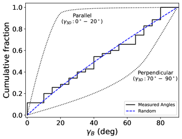
Figure 3: Cumulative distribution function (CDF) of plane of sky projected angles between the filaments and the ambient B-fields ($\gamma_{B}$). The blue dashed line shows the CDF of randomly distributed $\gamma_{3D}$ values. The two black dotted lines show expected CDF for parallel ($\gamma_{3D}\sim$0^∘–20^∘) and perpendicular distributions ($\gamma_{3D}\sim$70^∘–90^∘).

3.6 Filament Orientation Compared to Magnetic Fields

Geometrical configuration and alignment of the magnetic fields (hereafter B-fields) with filamentary structures could hint about the formation mechanisms of the filaments. Both numerical and observational studies have shown that B-fields are preferably oriented either perpendicular or parallel to the filaments depending on the column density ($N_{\rm{H_{2}}}$) of the filaments and strength of B-field (e.g., Li et al., 2013; Soler, 2019; Pillai et al., 2020; Jiao et al., 2024). The switch over from parallel to perpendicular orientation takes place at an $N_{\mathrm{H_{2}}}$ of 10${}^{21}-$10²² cm^-2. Simulations of Soler & Hennebelle (2017) showed that the transition from a parallel to a perpendicular field orientation is introduced by anisotropic converging flows regulated by a dynamically important magnetic field on larger scales. It is thus important to explore the relative orientation of filaments in reference to the ambient B-fields.

Plane-of-sky orientation of B-fields toward our target filaments were estimated using the Planck 353 GHz (870$\mu$m) dust continuum polarization observations. Stokes $I,Q,U$ maps were extracted from the Planck Public Data Release 2 (Planck Collaboration et al., 2016a, b). The maps have a pixel scale of $\sim 1\arcmin$ and beam size of $\sim 5\arcmin$. As our sole purpose of using Planck polarization data is obtaining the mean B-field orientation toward the filaments, the estimation of the position angles of the B-field was performed over a box with length equal to the length of the filament listed in Table 1 and a width of 6^′ around each filament. More technical details can be found in Baug et al. (2020).

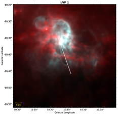
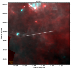
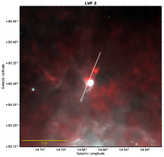
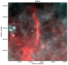
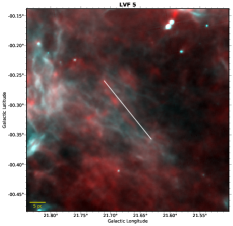
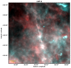
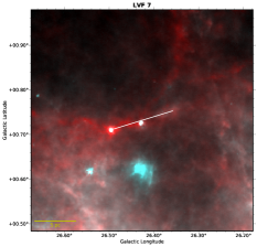
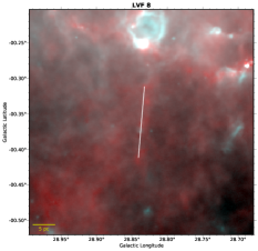
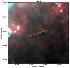
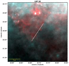
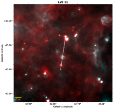
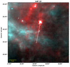
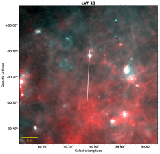
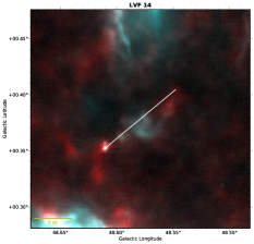
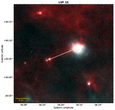
Figure 3: Two-color view of the linear filaments F1 to F15. Herschel 250 $\mu\mathrm{m}$/70 $\mu\mathrm{m}$ are shown in red/cyan. The filament is marked by end-to-end line in white.

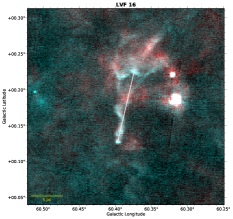
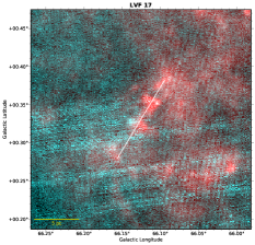
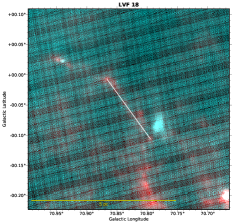
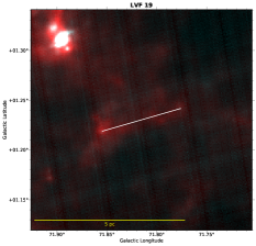
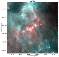
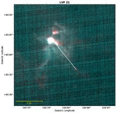
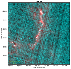
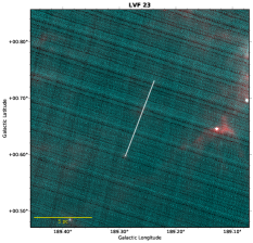
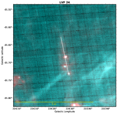
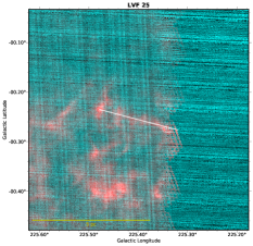
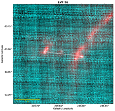
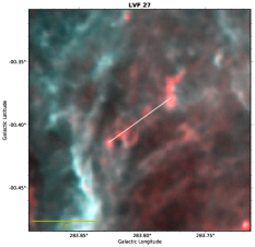
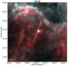
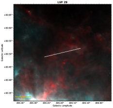
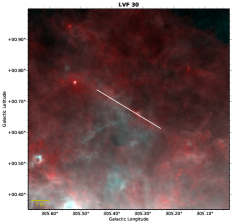
Figure 3: Continued for F16 to F30.

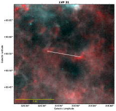
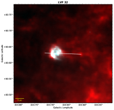
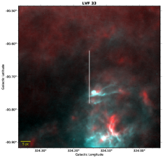
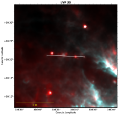
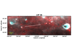
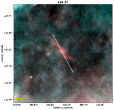
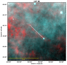
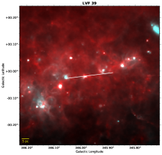
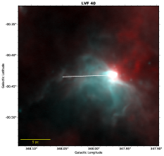
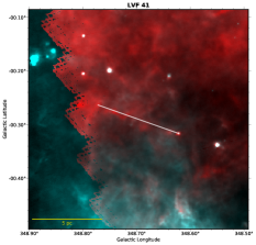
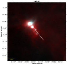
Figure 3: Continued for F31 to F42.

A cumulative histogram of the relative 2-dimensional position angles between the filaments and the corresponding B-fields ($\gamma_{B}$) is shown in Figure 3. Note that the calculated position angles are 2-dimensional projections of actual 3-dimensional angles. To examine the effect of projection on observed distribution of $\gamma_{B}$, we simulated about two million radially outward pairs of unit vectors randomly distributed on the surface of a sphere (see Stephens et al., 2017; Baug et al., 2020, for more details). Subsequently, we calculated their actual 3-dimensional angles ($\gamma_{3D}$) and also their 2-dimensional projection ($\gamma_{2D}$), assuming they are projected onto the y–z plane. These $\gamma_{2D}$ values could be considered as equivalent to the observed $\gamma_{B}$. Finally, we generated three different cumulative distribution functions (CDFs) of $\gamma_{2D}$, based on their actual 3-dimensional position angles – (1) parallel, with $\gamma_{3D}$ ranging between 0${}^{\circ}-$20^∘; (2) perpendicular, with $\gamma_{3D}$ ranging between 70${}^{\circ}-$90^∘; and (3) random, with $\gamma_{3D}$ for all possible angels ranging between 0${}^{\circ}-$90^∘. Along with the cumulative histogram of $\gamma_{B}$, three CDFs are also shown in Figure 3 for comparison.

No specific trend is noted in the cumulative histogram indicating toward a non-correlation of filaments with the large-scale B-field orientation. This is broadly consistent with the SOFIA (Stratospheric Observatory for Infrared Astronomy) observations of filament G47 (Stephens et al., 2022). However, we caution that the polarization data could largely be affected by line-of-sight depolarization (Planck Collaboration et al., 2016b) due to unknown B-field structure within the volume sampled by the beam. Also, averaging of multiple emitting layers with different position angles along the line-of-sight may lead to depolarization (Jones et al., 2015). Note that the angular resolution of the Planck data is comparable to the size of most of the filaments in our sample. The orientation of B-fields could vary substantially at the scale (and sub-scale) of filaments than they are in the larger scales, and the Planck data is incapable of resolving any such existing trends for the filaments in our sample. Dust polarization data at higher resolution are needed for a better comparison (e.g. Stephens et al., 2022).

4 Summary

We present the first catalog of 42 large-scale linear filaments across the full Galactic plane, and highlight some fundamental properties of them, including extreme linearity and velocity-coherence, velocity oscillation and filamentary gas flows, and diverse star formation activities. 1/3 of them are associated with the spiral arms, and 2/3 of them are located inter-arm, but only one is located at the arm center (a.k.a. Milky Way “bone”); none found near the Galactic center and in the Central Molecular Zone. A few filaments extend perpendicular to the Galactic plane while no obvious trend is found in orientation of the full sample. The filaments also appear to be randomly orientated compared to global magnetic fields.

As linear filaments are building blocks for more complex filamentary structure, these properties are important for further studies towards a unified understanding of more general filamentary structure, their role in star formation, and the structure of the Milky Way ISM.

Appendix A Supporting Materials

Table 1 lists physical properties of the 42 filaments, and Figure 4 shows distribution of some parameters. Figure 5 presents the MST, and Figure 3 illustrate the filaments in two-color far-IR views.

Table 1: Physical Properties of the Filaments

ID	$l_{1}$	$b_{1}$	$l_{2}$	$b_{2}$	$v_{\rm lsr}$	$d$	Len.	Le2e	Lmst	$w$	Aspect	$\Delta v$	Slope	Mass	Lum.	$L/M$	$T$	$N_{70}$	$N_{\rm cl}$	Linearity	$\theta$	$z$	Arm	$P_{\rm v}$	$\frac{P_{\rm v}}{P_{\rm cl}}$
	∘	∘	∘	∘	$\rm\frac{km}{s}$	kpc	∘	pc	pc	pc	ratio	$\rm\frac{km}{s}$	$\rm\frac{km/s}{pc}$	$M_{\odot}$	$L_{\odot}$	$\frac{L_{\odot}}{M_{\odot}}$	K				∘	pc		pc
(1)	(2)	(3)	(4)	(5)	(6)	(7)	(8)	(9)	(10)	(11)	(12)	(13)	(14)	(15)	(16)	(17)	(18)	(19)	(20)	(21)	(22)	(23)	(24)	(25)	(26)
F1	10.17	-0.36	10.18	-0.35	19.5	13.6	0.135	31.9	33.0	2.3	14.1	3.2	0.08	3.5E+04	8.7E+05	24.83	15.5	3	5	12.2	71	-100	Perseus
F2	12.0	-0.42	12.05	-0.42	45.3	12.0	0.187	39.2	39.5	2.4	16.4	4.3	-0.12	6.1E+03	5.6E+03	0.9	14.5	3	5	20.9	10	-87
F3	14.62	0.33	14.61	0.38	26.6	2.7	0.144	6.8	7.0	0.4	15.8	1.4	0.07	7.6E+02	2.6E+03	3.37	16.6	4	5	13.5	68	34		1.3	0.7
F4	18.07	0.55	18.07	0.57	23.3	13.7	0.09	21.5	22.0	2.1	10.6	1.2	0.06	2.4E+04	3.9E+03	0.16	12.4	0	5	10.5	89	125	Perseus	5.5	1.0
F5	21.7	-0.28	21.71	-0.26	85.3	10.6	0.149	27.6	28.1	2.2	12.9	1.7	-0.06	1.1E+04	3.3E+03	0.3	12.3	1	5	10.1	51	-53	Scu-Cen	7.5	1.1
F6	26.19	0.59	26.2	0.6	105.4	9.3	0.106	17.2	17.6	1.5	11.6	0.4	-0.01	1.4E+03	2.4E+03	1.73	16.2	0	5	12.3	74	98		4.5	1.0
F7	26.46	0.72	26.5	0.71	48.0	3.1	0.158	8.5	8.6	0.4	22.2	0.8	-0.01	7.3E+02	3.0E+03	4.16	15.3	2	5	23.8	17	59		2.5	1.2
F8	28.83	-0.33	28.83	-0.31	100.8	9.1	0.121	19.2	19.9	1.7	12.1	0.4	0.01	1.3E+04	2.0E+03	0.16	10.9	1	5	14.5	85	-49		8.45	1.7
F9	29.8	-0.83	29.81	-0.83	82.8	4.7	0.152	12.5	13.1	0.7	19.3	1.9	0.06	1.9E+03	2.8E+02	0.15	11.9	0	7	11.7	18	-50	Scu-Cen	2.3	1.1
F10	30.74	-0.89	30.73	-0.86	80.3	4.5	0.134	10.6	10.8	0.7	14.5	1.1	-0.1	1.7E+03	2.5E+02	0.15	11.4	1	5	13.3	56	-54		2.8	1.0
F11	32.74	-0.08	32.75	-0.06	36.9	11.7	0.154	31.5	32.8	1.5	22.2	1.8	-0.03	9.2E+03	2.0E+05	21.6	20.7	7	7	17.8	82	-22	Sag-Car	7.0	1.3
F12	36.88	-0.5	36.88	-0.47	59.7	9.8	0.099	16.8	17.2	1.3	13.0	2.0	0.09	1.0E+04	2.5E+04	2.5	12.4	2	5	10.1	79	-78	Sag-Car
F13	40.02	-0.12	40.02	-0.09	83.6	4.5	0.221	17.3	18.6	0.9	21.1	1.6	0.06	1.7E+03	2.9E+03	1.76	11.7	1	7	10.6	87	3		2.5	0.8
F14	48.6	0.36	48.61	0.35	35.9	8.6	0.102	15.3	15.7	1.6	10.0	1.4	0.1	4.5E+03	2.0E+03	0.44	13.1	1	5	10.6	40	72		3.8	1.0
F15	56.23	0.05	56.24	0.05	-4.2	9.6	0.113	19.0	21.3	1.2	17.9	1.7	0.07	7.6E+03	3.0E+04	3.95	14.0	4	6	12.1	22	27	Perseus
F16	60.38	0.18	60.37	0.23	20.3	6.4	0.128	14.3	14.4	1.5	9.7	1.1	-0.11	5.5E+02	7.3E+02	1.33	16.5	1	5	18.2	77	40
F17	66.1	0.38	66.09	0.38	16.0	4.9	0.136	11.7	11.9	0.7	17.6	2.7	-0.21	1.2E+03	1.4E+02	0.11	11.4	0	5	10.9	59	51
F18	70.85	-0.01	70.87	-0.01	9.1	1.2	0.147	3.2	3.3	0.3	13.0	1.4	-0.01	9.0E+01	1.1E+01	0.12	11.1	0	5	10.4	54	24
F19	71.83	1.22	71.85	1.22	15.2	1.9	0.103	3.4	3.5	0.3	10.3	0.9	-0.29	2.4E+02	4.2E+01	0.17	11.0	2	5	11.5	16	66
F20	80.66	1.28	80.68	1.26	-64.1	9.1	0.133	21.0	21.6	1.4	15.6	2.1	-0.11	2.3E+03	6.2E+03	2.73	17.3	5	6	10.6	22	232
F21	103.68	0.43	103.68	0.44	-61.5	4.2	0.108	8.0	8.1	0.5	15.7	1.9	0.24	2.8E+02	9.5E+02	3.38	14.5	3	5	11.2	51	61
F22	182.03	-0.23	182.02	-0.22	-10.4	4.4	0.146	11.1	11.7	0.7	17.1	0.8	-0.09	2.5E+03	2.1E+02	0.08	9.4	4	7	11.1	68	21
F23	189.25	0.71	189.24	0.73	10.4	2.8	0.16	7.8	8.0	0.4	19.1	1.1	-0.15	3.5E+02	3.4E+01	0.1	10.0	1	6	14.8	69	68	Perseus
F24	224.02	-1.67	224.03	-1.63	17.6	1.3	0.124	2.8	2.8	0.2	14.5	0.0	0.0	4.8E+01	4.4E+01	0.92	12.6	3	5	12.2	78	-9
F25	225.44	-0.24	225.48	-0.23	16.6	1.2	0.191	3.9	4.0	0.3	15.1	0.4	-0.04	1.4E+02	4.5E+00	0.03	8.6	0	5	19.4	15	23
F26	239.68	-0.8	239.68	-0.81	65.0	5.2	0.094	8.6	9.1	0.6	15.4	0.3	-0.04	2.1E+02	9.6E+01	0.47	13.4	2	5	12.3	7	-37	Perseus
F27	283.78	-0.38	283.78	-0.37	-2.6	5.5	0.091	8.8	9.2	1.3	7.2	0.0	0.0	7.8E+02	2.2E+03	2.82	20.0	1	5	11.7	36	-13	Sag-Car
F28	290.77	-1.43	290.77	-1.41	9.3	6.9	0.138	16.5	16.8	1.0	16.1	1.9	-0.15	9.2E+02	6.3E+03	6.86	13.8	1	5	15.9	69	-153
F29	305.22	0.5	305.26	0.49	-46.7	4.8	0.16	13.4	13.8	0.8	18.1	2.2	-0.14	2.6E+03	9.2E+02	0.35	12.8	3	6	10.7	14	63		2.6	0.9
F30	305.41	0.71	305.45	0.74	-46.5	4.9	0.257	22.1	23.4	0.7	32.9	1.5	0.06	2.9E+03	9.1E+02	0.32	11.7	2	9	10.4	31	78
F31	319.97	0.56	319.98	0.56	-40.1	2.5	0.121	5.3	5.5	0.5	11.8	1.2	0.03	2.8E+02	4.3E+01	0.15	10.9	0	5	11.4	10	45
F32	323.69	0.63	323.72	0.63	-46.9	10.6	0.134	24.8	26.6	1.9	14.4	1.5	0.04	5.3E+03	4.1E+04	7.7	16.9	3	6	11.3	2	124
F33	324.16	-0.66	324.15	-0.62	-33.3	9.6	0.183	30.6	30.9	2.0	15.6	1.2	0.0	5.2E+03	1.1E+03	0.22	12.4	0	5	13.4	90	-108
F34	328.81	0.07	328.81	0.07	-32.9	12.1	0.062	13.1	13.2	1.7	7.9	2.6	0.26	6.1E+03	2.6E+04	4.22	16.0	5	5	15.4	53	15		3.3	1.0
F35	338.56	0.22	338.58	0.21	-36.5	2.8	0.12	5.8	5.8	0.4	14.7	2.7	-0.11	7.7E+02	4.9E+03	6.38	17.8	4	5	17.6	3	30	Nor-Out	1.85	1.3
F36	338.82	-0.47	338.87	-0.48	-38.8	2.9	0.367	18.3	20.1	0.4	48.0	3.5	0.01	3.5E+03	4.2E+02	0.12	10.4	7	11	10.2	8	-4	Scu-Cen	2.0	1.0
F37	340.79	0.57	340.79	0.59	-124.9	9.4	0.144	23.5	24.2	1.6	14.9	0.8	-0.03	5.3E+03	1.6E+03	0.31	12.8	0	5	11.0	62	94
F38	342.93	-0.77	342.95	-0.75	-26.7	2.0	0.118	4.1	4.1	0.4	9.7	0.7	-0.14	1.4E+03	6.2E+01	0.04	8.9	1	5	15.8	44	-6	Nor-Out	1.14	1.1
F39	346.02	-0.02	346.06	-0.03	-80.3	10.8	0.189	35.7	36.8	1.4	25.8	2.8	-0.08	1.2E+04	6.4E+04	5.52	16.0	5	6	10.2	7	-1		4.0	0.5
F40	348.04	-0.44	348.05	-0.43	-94.7	6.0	0.104	10.9	11.1	1.1	10.3	2.1	-0.08	6.4E+03	4.3E+04	6.71	15.6	4	5	12.2	2	-33		3.0	1.1
F41	348.73	-0.29	348.77	-0.26	-19.3	2.2	0.184	7.1	7.1	0.4	16.1	0.7	-0.11	2.9E+02	1.3E+02	0.44	12.1	1	5	12.9	19	9		1.6	0.9
F42	352.62	-1.08	352.63	-1.07	-0.6	16.3	0.069	19.6	20.0	1.1	18.5	1.7	-0.09	5.1E+04	1.4E+06	27.86	21.9	5	5	12.7	51	-321	Sag-Car

Table 1: Continued.

ID	$l_{1}$	$b_{1}$	$l_{2}$	$b_{2}$	$v_{\rm lsr}$	$d$	Len.	Le2e	Lmst	$w$	Aspect	$\Delta v$	Slope	Mass	Lum.	$L/M$	$T$	$N_{70}$	$N_{\rm cl}$	Linearity	$\theta$	$z$	Arm	$P_{\rm v}$	$\frac{P_{\rm v}}{P_{\rm cl}}$
	∘	∘	∘	∘	$\rm\frac{km}{s}$	kpc	∘	pc	pc	pc	ratio	$\rm\frac{km}{s}$	$\rm\frac{km/s}{pc}$	$M_{\odot}$	$L_{\odot}$	$\frac{L_{\odot}}{M_{\odot}}$	K				∘	pc		pc
(1)	(2)	(3)	(4)	(5)	(6)	(7)	(8)	(9)	(10)	(11)	(12)	(13)	(14)	(15)	(16)	(17)	(18)	(19)	(20)	(21)	(22)	(23)	(24)	(25)	(26)
Min	-177.97	-1.67			-124.9	1.2	0.062	2.8	2.8	0.2	7.2	0.0	0.00	4.8E+01	4.5E+00	0.03	8.6	0.0	5.0	10.1	1.9	-320.5		1.1	0.5
Max	103.68	1.28			105.4	16.3	0.367	39.2	39.5	2.4	48.0	4.3	0.29	5.1E+04	1.4E+06	27.86	21.9	7.0	11.0	23.8	90.0	232.2		8.5	1.7
Avg	-8.92	-0.05			4.8	6.7	0.142	15.5	16.0	1.1	16.2	1.5	0.08	5.8E+03	6.6E+04	3.47	13.7	2.2	5.6	13.1	44.5	6.8		3.6	1.0
Med	1.40	-0.05			9.9	5.4	0.135	13.9	14.1	1.0	15.3	1.5	0.07	2.1E+03	2.0E+03	0.69	12.8	2.0	5.0	12.2	51.2	18.0		2.8	1.0
Std	66.76	0.66			54.0	4.0	0.053	9.4	9.7	0.6	7.0	0.9	0.07	9.9E+03	2.6E+05	6.41	3.1	2.0	1.2	3.2	29.3	88.2		2.1	0.2
Skewness	-0.9	-0.2			-0.1	0.5	2.1	0.7	0.7	0.5	2.7	0.7	1.2	3.3	4.7	2.9	0.7	0.8	3.0	1.6	0.0	-1.0		1.1	0.8
Kurtosis	0.5	-0.1			-0.3	-0.8	7.5	-0.1	-0.3	-0.9	10.4	0.8	1.4	12.1	22.5	8.1	0.3	-0.2	10.2	2.3	-1.5	4.1		0.4	3.2