Intuitive Fine-Tuning:
Towards Simplifying Alignment into a Single Process

Abstract

Supervised Fine-Tuning (SFT) and Preference Optimization (PO) are two fundamental processes for enhancing the capabilities of Language Models (LMs) post pre-training, aligning them better with human preferences. Although SFT advances in training efficiency, PO delivers better alignment, thus they are often combined. However, common practices simply apply them sequentially without integrating their optimization objectives, ignoring the opportunities to bridge their paradigm gap and take the strengths from both. To obtain a unified understanding, we interpret SFT and PO with two sub-processes — Preference Estimation and Transition Optimization — defined at token level within the Markov Decision Process (MDP) framework. This modeling shows that SFT is only a specialized case of PO with inferior estimation and optimization. PO evaluates the quality of model’s entire generated answer, whereas SFT only scores predicted tokens based on preceding tokens from target answers. Therefore, SFT overestimates the ability of model, leading to inferior optimization. Building on this view, we introduce Intuitive Fine-Tuning (IFT) to integrate SFT and Preference Optimization into a single process. IFT captures LMs’ intuitive sense of the entire answers through a temporal residual connection, but it solely relies on a single policy and the same volume of non-preference-labeled data as SFT. Our experiments show that IFT performs comparably or even superiorly to sequential recipes of SFT and some typical Preference Optimization methods across several tasks, particularly those requires generation, reasoning, and fact-following abilities. An explainable Frozen Lake game further validates the effectiveness of IFT for getting competitive policy. Our code will be released at https://github.com/TsinghuaC3I/Intuitive-Fine-Tuning.

1 Introduction

Large Language Models (LLMs) have demonstrated remarkable powerful potential across various downstream tasks after pre-training on large-scale corpora brown2020language ; achiam2023gpt ; zhou2024generative . However, their instruction-following skills and trustworthiness still fall short of expectations bender2021dangers ; bommasani2021opportunities ; li2022trust . Therefore, algorithms such as Supervised Fine-Tuning (SFT) and Reinforcement Learning from Human Feedback (RLHF) ziegler2019fine ; ouyang2022training ; lee2023rlaif are used to further enhance LLMs’ abilities and align them better with human preferences.

Considering the limited effectiveness of SFT and the high cost of data construction and training computation for RLHF, these two methods are often combined to leverage their respective strengths. Unfortunately, they are typically implemented as a sequential recipe constrained by the paradigm gap between SFT and early RLHF methods, stemming from differences in loss functions, data formats, and the requirement for auxiliary models.

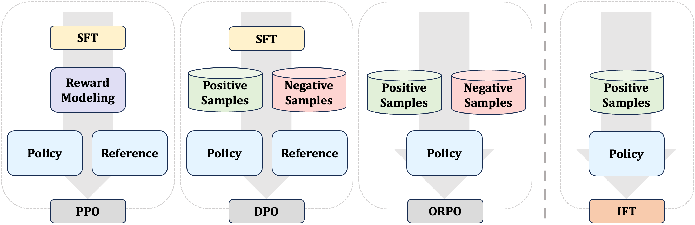
Figure 1: Comparison of Alignment Methods. IFT conducts alignment solely relying on positive samples and a single policy, starting from a pre-trained base model. IFT not only shows high efficiency as SFT, but also performs comparably or even superiorly to other alignment algorithms.

Recently, Direct Preference Optimization (DPO) rafailov2024direct was proposed to integrate Reward Modeling and Policy Optimization into one single procedure using a loss function derived from Proximal Policy Optimization (PPO) schulman2017proximal . This approach demonstrates the potential to unify SFT and RLHF for the first time. Henceforth, many extended methods have been tried to realize this objective by bridging the gap between SFT and DPO. Some of them ethayarajh2024kto ; hong2024reference ; zhang2024negative aim to transform the contrastive loss of DPO into a SFT-like cross-entropy loss, learning positive samples similar to SFT while unlearning negative samples resort to Unlikelihood Training welleck2019neural . Some others get rid of the preference-labeling process before training, switching to collect samples and labels/rewards in an online manner liu2023statistical ; yuan2024self ; guo2024direct ; calandriello2024human ; tajwar2024preference , or just treating the SFT targets and online policy generations as positive and negative samples respectively xiong2023iterative ; chen2024self ; mitra2024orca ; liu2024extensive . Nevertheless, preference-labeled pairwise data is still essential in these methods, and the need for reference model only becomes unnecessary in some cases. Thus the core differences between SFT and Preference Optimization are not eliminated thoroughly. To address this challenging issue, a deeper and more unified understanding of them are needed.

In this paper, we attempt to explain the similarities and differences between SFT and Preference Optimization by defining Preference Estimation and Transition Optimization in terms of state-action pairs within the Markov Decision Process (MDP) framework. Through this modeling, we demonstrate that SFT is simply a specialized case with inferior estimation and optimization among all Preference Optimization methods. To be specific, typical Preference Optimization methods usually sample the entire answer of policy based solely on the initial instruction, and align the policy preference reflected by the sampled sentence with human preferences. In contrast, SFT only samples a single token based on intermediate state of target answer, which leads to a biased estimation of policy preference and an inferior alignment shortcut. Or put it in a metaphorical view, when preparing for an exam, it is obviously more beneficial to review reference answers after completing entire questions, rather than trying to infer each subsequent step based on the reference answer ahead and checking it immediately. It is the similar case in LMs’ training, where SFT is less beneficial for enhancing LMs.

Depending on this understanding, we introduce a unified alignment algorithm named Intuitive Fine-Tuning (IFT), which builds policy preference estimation in an intuitive manner like human, who can have a vague sense of the complete answer after hearing a question. Through a closer estimation to truly policy preference than SFT, IFT achieves a comparable or even superior alignment performance compared to the sequential recipe of SFT and Preference Optimization. Additionally, IFT requires only a single policy model, and the same volume and format of data as SFT, enjoying both data and computation efficiency. These characteristics also enable IFT to be implemented in domains where preference data is unavailable or expensive to collect.

Our main contribution are three folds: 1) By modeling within the MDP framework, we explain the similarities and differences between SFT and two fundamental Preference Optimization methods, PPO and DPO; 2) Based on this modeling, we introduce Intuitive Fine-tuning (IFT), a deeply unified version of SFT and Preference Optimization. IFT utilizes temporary residual connections to extract the model’s generation preference given the initial instructions, offering similar efficiency to SFT while achieving performance closer to Preference Optimization; 3) Through experiments on several benchmarks, we validate that IFT performs comparably or even superiorly to various SFT recipes and existing Preference Optimization methods. In particular, IFT demonstrates significantly stronger reasoning and fact-following abilities than the chosen baselines. An explainable toy-setting Frozen Lake further demonstrates the effectiveness of IFT.

2 Related Work

Classical Reinforcement learning (RL) has demonstrated strong performance in various sequential decision-making and optimal control domains, including robotics levine2018learning , computer games vinyals2019grandmaster and others guan2021direct . There are two main categories of RL algorithms: value-based and policy-based, depending on whether they learn a parameterized policy. Value-based RL aims to fit an value function defined by Bellman Equation, containing methods such as Monte-Carlo (MC) Learning lazaric2007reinforcement and Temporal Difference Learning sutton1988learning ; seijen2014true . However, value-based methods struggle in continuous or large discrete space for its greedy objective. Thus, policy-based methods were introduced to model the decision-making process using a parameterized policy. As one of its best-known algorithms, Proximal Policy Optimization (PPO) schulman2017proximal is widely used in various domains, including Natural Language Processing (NLP).

Alignment for LMs has emerged as a crucial task these years, which adjusts the LMs’ generation distribution in line with human preferences. Building on the Bradley-Terry (BT) bradley1952rank Model, current alignment methods typically train models to distinguish positive and negative answers given the same instruction using RLHF/RLAIF ziegler2019fine ; ouyang2022training ; lee2023rlaif . While PPO remains the primary algorithm for alignment, its high demands for computation and memory hinders its broader use. Consequently, many improved methods have been proposed dong2023raft ; yuan2023rrhf ; zhao2023slic . Among them, DPO rafailov2024direct unifies reward modeling and policy optimization by utilizing a loss function derived from PPO, training a single model to serve as both a policy model and a reward model. Without sacrificing performance, DPO decrease the costly consumption of PPO through directly value iteration similar to a preference-based format of MC instead of TD. Nevertheless, the expensive preference-labeling process is still required. Additionally, a warm-up stage based on SFT is also necessary, which may bring trade-offs in fitting different objectives between SFT and Preference Optimization.

Improved Versions of DPO come out one after another. Efforts such as liu2023makes ; khaki2024rs ; yin2024relative ; guo2024controllable ; bansal2024comparing ; liu2024extensive try to enhance the contrastive learning by utilizing better ranking strategies, more informative data, or more number of negative samples. except for using offline data, liu2023statistical ; yuan2024self ; guo2024direct ; calandriello2024human ; chen2024self ; mitra2024orca focus on online sampling and automated label/reward collection, reducing the manual cost required for alignment. Recently, methods like ethayarajh2024kto ; hong2024reference aim to reduce DPO’s dependency on SFT warm-up by transforming its loss functions and data format into a SFT manner. These algorithms handle positive and negative samples using SFT objective and Unlikelihood Training welleck2019neural , respectively. However, the actual volume of training data is not decreased in these methods. Also, GPU-memory-consuming pair-wise data is still required, while the need for a reference model and preference-labeling for the entire answer trajectory is only eliminated in limited cases.

3 Preliminaries

3.1 MDP in Language Models

The MDP applied to LMs can be formally described as a tuple $\mathcal{M}=(\mathcal{S},\mathcal{A},\mathcal{T},r,\rho_{0})$, where $\mathcal{S}$ is the state space comprising ordered permutations of vocabularies, $\mathcal{A}$ is the action space consisting of vocabularies defined by the tokenizer, $\mathcal{T}$ is the transition matrix indicating token generation probabilities for given states, $r$ represents rewards for state-action pairs, and $\rho_{0}$ is the initial state typically based on given instructions. See more details in Appendix A.1.

The primary objective of Language Modeling is to train a policy $\pi_{\theta}$ with $\mathcal{T}_{\theta}$ to mimic a human policy $\pi^{*}$ with $\mathcal{T}^{*}$, aiming for the two transition matrices to become identical:

$$\forall s\in\mathcal{S},a\in\mathcal{A}:\mathcal{T}_{\theta}(a|s)\rightarrow\mathcal{T}^{*}(a|s)$$ (1)

This process can also be expressed using another state-state transition matrix $T$:

$$\forall~{}s,s^{\prime}\in S:T_{\theta}(s^{\prime}|s)\rightarrow T^{*}(s^{\prime}|s)$$ (2)

where $T$ is equivalence to $\mathcal{T}$, but instead, indicating the transition probability between states.

3.2 Preference Estimation

We define the preference $\mathcal{P}$ of policy $\pi$ given an initial instruction $\rho_{0}$ as a mapping:

$$\mathcal{P}(\rho_{0}):\rho_{0}\rightarrow[\pi(\rho_{0}),\pi(s_{1}),\pi(s_{2}),...]$$ (3)

where $s_{i+1}=[s_{i},a_{i}]$ , $a_{i}=\pi(s_{i})$ and $s_{0}=\rho_{0}$.

During alignment, the model preference gradually approaches the human preference:

$$\mathcal{P_{\theta}}(\rho_{0})\rightarrow\mathcal{P^{*}}(\rho_{0}):\bigg{\{}\begin{aligned} &\mathcal{P_{\theta}}(\rho_{0}):\rho_{0}\rightarrow[\pi_{\theta}(\rho_{0}),\pi_{\theta}(s_{1}^{\theta}),\pi_{\theta}(s_{2}^{\theta}),\ldots]\\ &\mathcal{P^{*}}(\rho_{0}):\rho_{0}\rightarrow[\pi^{*}(\rho_{0}),\pi^{*}(s_{1}^{*}),\pi^{*}(s_{2}^{*}),\ldots]\end{aligned}$$ (4)

As the truly preferences are difficult to obtain, alignment is usually conducted based on the Preference Estimation of model and human, denoted as $\hat{\mathcal{P}_{\theta}}$ and $\mathcal{\hat{P^{*}}}$ respectively. The estimations from some common methods are listed in Table 1.

To make preference optimizable, the policy’s preference can also be expressed as follows:

$$\mathcal{P}(\rho_{0})=\{\mathcal{T}(a|s)|\forall a\in\mathcal{A},s\in\mathcal{S}_{\rho_{0}}\}$$ (5)

Here, $\mathcal{S}_{\rho_{0}}$ denotes a conditional state space that constrained by the initial state $\rho_{0}$, within which each state can only be initially derived from $\rho_{0}$. Consequently, the model preference can be optimized through transition matrix, named Transition Optimization.

3.3 Transition Optimization

Ideally, we want to align the state-action transition matrix between model and human in a $\rho_{0}$-constrained state space:

$$\forall a\in\mathcal{A},s\in\mathcal{S}_{\rho_{0}}:\mathcal{T}_{\theta}(a,s)\rightarrow\mathcal{T^{*}}(a,s)$$ (6)

which is equivalent to the following format expressed by state-state transition matrix:

$$\forall s\in\mathcal{S}_{\rho_{0}}:T_{\theta}(s,\rho_{0})\rightarrow T^{*}(s,\rho_{0})$$ (7)

However, considering the limited data, only matrix elements representing state-action/state-state pairs contained in the dataset $\mathcal{D}$ would be aligned. Given a data sample with instruction $\rho_{0}$ and target answer with length-$N$, the objective would be:

$$\forall a\in\mathcal{A},n\in[0,N],\rho_{0}\in\mathcal{D},s_{n}^{*}\in\mathcal{S}_{\rho_{0}}^{*}:\mathcal{T}_{\theta}(a,s_{n}^{*})\rightarrow\mathcal{T^{*}}(a,s_{n}^{*})$$ (8)

Or equivalent to:

$$\forall n\in[0,N],\rho_{0}\in\mathcal{D},s_{n}^{*}\in\mathcal{S}_{\rho_{0}}^{*}:T_{\theta}(s_{n}^{*},\rho_{0})\rightarrow T^{*}(s_{n}^{*},\rho_{0})$$ (9)

$$T_{\theta}(s_{n}^{*}|\rho_{0})=\prod\limits_{i=0}^{n}\mathcal{T}_{\theta}(a_{i}^{*}|s_{i}^{*}),~{}T^{*}(s_{n}^{*}|\rho_{0})=\prod\limits_{i=0}^{n}\mathcal{T^{*}}(a_{i}^{*}|s_{i}^{*})$$ (10)

where $s_{0}^{*}=\rho_{0}$, $T^{*}(\rho_{0}|\rho_{0})=T_{\theta}(\rho_{0}|\rho_{0})=1$, and $s_{i}^{*}$ denotes the intermediate state of target answer.

Consequently, the loss function can be derived from the disparities of the transition matrices between model and human. Some typical loss function are listed in Appendix A.4

Table 1: Reformulation of SFT, PPO and DPO

Method Preference Estimation Transition Optimization $\hat{s_{n}^{*}}$ in $\hat{\mathcal{P^{*}}}$ $\hat{s_{n}^{\theta}}$ in $\hat{\mathcal{P_{\theta}}}$ Truly $s_{n}^{*}$ $s_{n}^{\theta}$ $T_{\theta}(s_{n}^{*},\rho_{0})\rightarrow T^{*}(s_{n}^{*},\rho_{0})$ SFT $s_{n}^{*}$ $s_{n}^{*}$ $T_{\theta}(s_{n}^{*},s_{n-1}^{*})\rightarrow T^{*}(s_{n}^{*},s_{n-1}^{*})$ PPO $s_{n}^{\theta}$ $s_{n}^{\theta}$ $T_{\theta}(\hat{s_{n}^{*}},s_{n-1}^{\theta})\rightarrow T^{*}(\hat{s_{n}^{*}},s_{n-1}^{\theta})$ DPO online $s_{n}^{*}$ $s_{n}^{\theta}$ $T_{\theta}(s_{n}^{*},\rho_{0})\rightarrow T^{*}(s_{n}^{*},\rho_{0})$ offline $s_{n}^{*}$ $s_{n}^{\theta^{-}}$ $\hat{T_{\theta}}(s_{n}^{*},\rho_{0})\rightarrow T^{*}(s_{n}^{*},\rho_{0})$

3.4 From SFT to Preference Optimization

We reformulate SFT, PPO and DPO using the aforementioned framework, detailed in Table 1 and Appendix A.4. A more comprehensible version is presented in Figure 2. To compare the differences between them, we begin by introducing a fundamental theorem and corollary:

Theorem Given a set of events $\mathcal{Z}$, the probability of any event $z\in\mathcal{Z}$ is between 0 and 1, i.e., $\forall z\in\mathcal{Z}:0\leq P(z)\leq 1$. If all events are mutually independent, the sum of their probabilities equals 1, i.e., $1=\sum_{z\in\mathcal{Z}}P(z)$. The event $z^{*}$ with the highest probability has a probability greater than or equal to any other event, i.e., $\forall z\in\mathcal{Z}:0\leq P(z)\leq P(z^{*})\leq 1$.

Corollary LMs consistently assign higher probabilities to their own greedy predictions than to human preference:

$$\forall s\in S:\mathcal{T}_{\theta}(\pi^{*}(s),s)\leq\mathcal{T}_{\theta}(\pi_{\theta}(s),s)\leq 1$$ (11)

thus LMs tend to assign higher probabilities to its own generation than to target answer given the same initial instruction:

$$\forall n\in[0,N],s_{n}^{*}\in\mathcal{S}_{\rho_{0}}^{*},s_{n}^{\theta}\in\mathcal{S}_{\rho_{0}}^{\theta}:T_{\theta}(s_{n}^{*},\rho_{0})\leq T_{\theta}(s_{n}^{\theta},\rho_{0})\leq 1$$ (12)

where $N$ represents the length when the generation reaches the EOS token or the truncation length.

SFT provides an unbiased estimation of human preference, but a biased estimation for model:

$$\hat{\mathcal{P_{\theta}}}(\rho_{0}):\rho_{0}\rightarrow[\pi_{\theta}(\rho_{0}),\pi_{\theta}(s_{1}^{*}),\pi_{\theta}(s_{2}^{*}),\ldots]$$ (13)

which is caused by wrong prior state when predicting each subsequent token. Consequently, the Transition Optimization objective of SFT:

$$T_{\theta}(s_{n}^{*},s_{n-1}^{*})\rightarrow T^{*}(s_{n}^{*},s_{n-1}^{*})$$ (14)

secretly sets $T_{\theta}(s_{n-1}^{*},\rho_{0})=1$ during aligning $T_{\theta}(s_{n}^{*},\rho_{0})$ with $T^{*}(s_{n}^{*},\rho_{0})$. This makes an overestimation of the transition probabilities and preference of model, leading to an inferior optimization progress in SFT. Thus Preference Optimization is needed for further preference alignment.

PPO shows an unbiased estimation of model preference, while employing a progressively unbiased estimation of human preference:

$$\hat{\mathcal{P^{*}}}(\rho_{0}):\rho_{0}\rightarrow[\pi^{*}(\rho_{0}),\pi^{*}(s_{1}^{\theta}),\pi^{*}(s_{2}^{\theta}),\ldots]$$ (15)

Initially biased, this estimation gradually becomes unbiased as the model aligns with human preference over time. As $T_{\theta}(s_{n}^{\theta},\rho_{0})$ is consistently closer to 1 than $T_{\theta}(s_{n-1}^{*},\rho_{0})$, PPO provides an closer approximation than SFT to the actual circumstances of model in Transition Optimization:

$$T_{\theta}(\hat{s_{n}^{*}},s_{n-1})\rightarrow T^{*}(\hat{s_{n}^{*}},s_{n-1})$$ (16)

which sets $T_{\theta}(s_{n}^{\theta},\rho_{0})=1$ and $\hat{s_{n}^{*}}=\pi^{*}(s_{n-1}^{\theta})$. However, estimating $\pi^{*}(s_{n-1}^{\theta})$ is at the expense of preference-labeling, reward modeling and online sampling.

DPO theoretically achieves the best estimation across all scenarios, even without reward modeling. However, obtaining pairwise preference data online is costly, as it requires real-time negative sampling from model and preference labeling by human. Thus, mainstream implementations often rely on off-policy negative samples out-of-distribution from the optimized model, which may yield unstable and sub-optimal results due to biased preference estimation and inferior transition optimization.

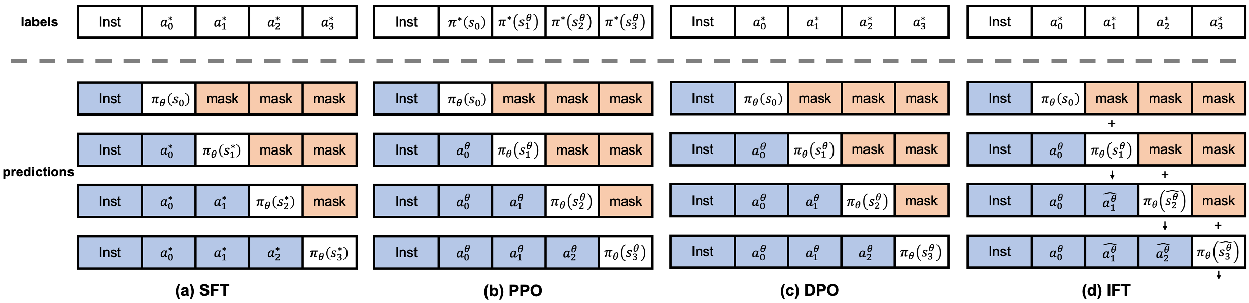
Figure 2: The Training Paradigm of Different Methods. Symbol $*$ and $\theta$ denote human and model respectively, with $a_{i}^{*}=\pi^{*}(s_{i}^{*})$ and $s_{i+1}^{*}=[s_{i}^{*},a_{i}^{*}]$, similarly for $\theta$. SFT uses priors deviating from model distribution, resulting in a more biased estimation of model preferences compared to PPO and DPO. IFT achieves a closer estimation than SFT by utilizing temporary residual connections, while maintaining the data and computational efficiency as SFT.

4 Method

While SFT is data and computation-efficient, it has an inferior approximation for both Preference Estimation and Transition Optimization. In the other side, Preference Optimization (represented by PPO and DPO) enjoys better approximation at the expense of preference data construction. We hope to make good use of their strength, using solely the target data as SFT but having similar approximation as Preference Optimization.

4.1 Intuitive Preference Estimation

A key distinction between SFT and Preference Optimization lies in whether the full distribution of model preference for each initial instruction is sampled. Contrasted to Preference Optimization, the intermediate state of the target answer used for prior in SFT may be far away from the model preference, leading to inferior outcomes.

To obtain a state estimation $\hat{s_{i}^{\theta}}$ closer to model preference, we introduce a model-based distribution disturbance function $\delta_{\theta}$ for the biased state:

$$\hat{s_{i}^{\theta}}=\delta_{\theta}(s_{i}^{*})\\ =(1-\lambda)s_{i}^{*}+\lambda\pi_{\theta}(s_{i-1}^{*})$$ (17)

which can also be interpreted as a temporal residual connection. Through this approach, model can predict not only the next token from intermediate state of target answer, but also develop an intuitive sense to the entire answer generation solely based on the initial instruction, deriving more accurate Preference Estimation for model:

$$\hat{\mathcal{P_{\theta}}}(\rho_{0})=[(1-\lambda)\mathcal{P_{\theta}}^{sft}+\lambda\mathcal{P_{\theta}}^{truly}](\rho_{0})$$ (18)

4.2 Dynamic Relation Propagation

With improved Preference Estimation, we achieve a Transition Optimization process closer to the original objective:

$$\forall n\in[0,N],\rho_{0}\in\mathcal{D},s_{n}^{*}\in\mathcal{S}_{\rho_{0}}^{*}:\hat{T_{\theta}}(s_{n}^{*},\rho_{0})\rightarrow T^{*}(s_{n}^{*},\rho_{0})$$ (19)

where $s_{0}^{*}=\rho_{0}$ and $\hat{T_{\theta}}(s_{n}^{*},\rho_{0})=\prod\limits_{i=0}^{n-1}T_{\theta}(s_{i+1}^{*},\hat{s_{i}^{\theta}})$. This objective can be optimized by the following loss function that quantifies the disparities of transition between model and human:

$$\mathcal{L}(\hat{T_{\theta}};T^{*})=\mathbb{E}_{\rho_{0}\sim\mathcal{D}}\mathbb{E}_{s_{n}^{*}\sim\mathcal{S}_{\rho_{0}}^{*}}\left[\sum\limits_{n=0}^{N}\log\frac{\hat{T_{\theta}}(s_{n}^{*},\rho_{0})}{T^{*}(s_{n}^{*},\rho_{0})}\right]$$ (20)

We make the same hypothesis as SFT that the optimization objective of each target intermediate state has a probability equal to 1:

$$\forall n\in[0,N],\rho_{0}\in\mathcal{D},s_{n}^{*}\in\mathcal{S}_{\rho_{0}}^{*}:T^{*}(s_{n}^{*},\rho_{0})=1=T^{*}(s_{N}^{*},\rho_{0})$$ (21)

Then, the loss function can be reformulated as:

$$\mathcal{L}_{\text{IFT}}(\mathcal{T}_{\theta},\delta_{\theta})=\mathbb{E}_{\rho_{0}\sim\mathcal{D}}\mathbb{E}_{s_{i}^{*}\sim\mathcal{S}_{\rho_{0}}^{*}}\left[-\sum\limits_{n=0}^{N}\sum\limits_{i=n}^{N}\log\mathcal{T}_{\theta}(a_{i}^{*},\delta_{\theta}(s_{i}^{*}))\right]$$ (22)

where $a_{i}^{*}=\pi^{*}(s_{i}^{*})$. This reformulation facilitates parallel implementation, allowing IFT to achieve computational efficiency similar to SFT. See Appendix A.2 for complete derivation.

At the same time, we also prove that the objective optimized by this loss function implicitly satisfies the Bellman Equation for each state:

$$V_{\theta}(\hat{s_{n}^{\theta}})=\exp\bigg{(}-\mathcal{L}\big{(}\hat{T_{\theta}}(s_{n}^{*},\rho_{0})\big{)}\bigg{)}$$ (23)

The derivation is in Appendix A.3. This proof guarantees the optimization process closer to RLHF. Additionally, it ensures the optimized objective not only reflects the prediction accuracy of current token, but also considers the influence of the current selection on future generation, helping model acquire an intuitive understanding of generation, and a better causality for reasoning and fact-following. Additionally, a decay factor can be incorporated, as in the typical Bellman Equation, to ensure effectiveness in long trajectories.

5 Experiments

We conduct experiments mainly on NLP setting. Considering the absence of an optimal policy of human language generation, we also utilize the Frozen Lake environment for further validation.

5.1 Settings for NLP

Datasets. We select UltraChat-200k ding2023enhancing and UltraFeedback-60k cui2023ultrafeedback as single-target and pair-wise dataset respectively.

Models. We conduct experiments on Mistral-7B-v0.1 jiang2023mistral and Mistral-7B-sft-beta tunstall2023zephyr , with the former as the base model and the latter fine-tuned on UltraChat-200k.

Scenarios. We consider two different training scenarios, one using Preference Optimization exclusively, and the other employing sequential recipe of SFT and Preference Optimization. In the first scenario, alignment is conducted directly from base model Mistral-7B-v0.1 using UltraFeedback. In order to ensure balanced data volume between different method, we randomly sample 60k data from UltraChat as supplementary for SFT and IFT, for only the target data are utilized in these two methods. The second scenario is commonly seen, where SFT and Preference Optimization is employed sequentially. For this scenario, we use Mistral-7B-sft-beta as start-point, which has been fine-tuned with UltraChat using SFT. Then we fine-tune it further with UltraFeedback using Preference Optimization.

Baselines. Our main baselines are SFT and DPO rafailov2024direct , with PPO excluded due to computational limitations. Additionally, we incorporate an improved versions of DPO, named ORPO hong2024reference , who claims to achieve alignment directly without SFT and reference model, aligning well with our goals. In addition to reproducing the algorithms mentioned above, we also consider Zephyr-7B-beta tunstall2023zephyr and Mistral-ORPO-alpha hong2024reference , two open-source checkpoints that utilize sequential and direct recipes respectively. Both of them used start-point models and datasets similar to ours.

Benchmarks. We consider two types of benchmarks. One is from the widely used Open-LLM LeaderBoard, which contains ARC-Challenge (25-shot) clark2018think , MMLU (5-shot) chung2024scaling , TruthfulQA (0-shot) lin2021truthfulqa , WinoGrande (5-shot) sakaguchi2021winogrande , and GSM8K (5-shot) cobbe2021training . The other is LM-based evaluation, including Alpaca-Eval and Alpaca-Eval-2 dubois2024alpacafarm . We utilize chat template for all benchmarks to obtain a more accurate evaluation for chat models.

5.2 Main Results in NLP Tasks

Effectiveness on Sequential Recipe. In this scenario, IFT demonstrates good performance across benchmarks having standard answers or not, see more details in Table 2 and 3. On Open-LLM Leaderboard, IFT showcases the best average capabilities across all tasks, excelling particularly in tasks requiring generation, reasoning and fact-following abilities, such as TruthfulQA and GSM8K. However, IFT has a relatively large gap between DPO in multi-choice tasks like ARC-Challenge and MMLU. We will explained the reasons later. When evaluated for instruction-following and question-answering abilities as judged by GPT-4, IFT’s performance is comparable to that of the chosen baselines. Remarkably, IFT achieves these results using the least amount of data and computational resources among all the methods tested.

Table 2: Evaluation on LLM-based Benchmarks. In the typical sequential setting, SFT+DPO still achieves the highest scores, although IFT performs comparably. However, when aligning directly from the base model, IFT performs not only superiorly to other methods but also on par with sequential recipes. As for open-source models, we directly present its publicly available score.

Method Reference Data Alpaca-Eval Alpaca-Eval-2 pairwise volume win-rate lc win-rate win-rate lc win-rate Mistral-7B – – – 24.72 11.57 1.25 0.35      fine-tuning with UltraFeedback-60k + SFT ✗ ✗ 120k 82.56 78.32 7.09 8.67 + DPO ✓ ✓ 120k 74.00 73.12 9.73 8.58 + ORPO ✗ ✓ 120k 85.14 76.60 8.82 12.34 + IFT ✗ ✗ 120k 85.18 78.78 9.95 13.27 Mistral-ORPO-$\alpha$ ✗ ✓ 120k 87.92 – – 11.33      fine-tuning with UltraChat-200k + UltraFeedback-60k sequentially + SFT ✗ ✗ 200k 86.69 77.96 4.08 6.43 + SFT + SFT ✗ ✗ 260k 86.34 76.98 4.55 7.14 + SFT + DPO ✓ ✓ 320k 91.62 81.54 10.08 13.72 + SFT + ORPO ✗ ✓ 320k 86.26 79.67 7.40 12.27 + SFT + IFT ✗ ✗ 260k 88.37 81.29 10.26 14.34 Zephyr-7B-$\beta$ ✓ ✓ 320k 90.60 – – 10.99

Table 3: Evaluation on Open-LLM Leaderboard with chat template. When fine-tuning with the same recipe, IFT achieves the highest average score across all methods. Directly conducting alignment using IFT showcases the best performance in all recipes with the least data and computation.

Method ARC ARC-Gen MMLU TruthfulQA WinoGrande GSM8K Avg. Mistral-7B 53.07 73.04 59.14 45.29 77.58 38.89 54.79      fine-tuning with UltraFeedback-60k + SFT 56.49 74.00 60.44 55.57 77.90 42.84 58.65 + DPO 61.86 73.54 61.02 47.98 76.64 43.89 58.28 + ORPO 56.66 73.98 60.57 51.77 77.19 42.30 57.70 + IFT 56.74 74.15 60.49 57.65 78.45 44.73 59.61 Mistral-ORPO-$\alpha$ 57.25 73.72 58.74 60.59 73.72 46.78 59.41      fine-tuning with Ultrachat-200k + UltraFeedback-60k sequentially + SFT 57.68 72.87 58.25 45.78 77.19 40.94 55.97 + SFT + SFT 58.10 72.61 58.40 48.59 76.80 43.06 56.99 + SFT + DPO 63.91 73.98 59.75 46.39 76.06 41.47 57.52 + SFT + ORPO 58.45 73.21 58.80 50.31 76.45 42.76 57.35 + SFT + IFT 58.36 73.38 58.45 52.39 78.06 43.82 58.22 Zephyr-7B-$\beta$ 67.41 72.61 58.74 53.37 74.11 33.89 57.50

Effectiveness of Preference Optimization Alone. IFT not only maintains the performance advantages compared with other baselines in this setting, as seen in the sequential scenario. But also, IFT performs comparably or even superiorly to many method in sequential recipe. While DPO tends to fail under this setting, ORPO remains competitive in its open-source model. However, when constrained in the same experiment setting, the performance of ORPO becomes worse than IFT. Additionally, the reliance on preference data makes ORPO more costly in terms of negative sampling, preference labeling, and GPU memory consumption. Consequently, IFT stands out as a more efficient and cost-effective alternative in this context.

Multi-Choice vs. Generation. IFT performs better on generation tasks but struggles with multi-choice, whereas DPO exhibits the opposite performance. This may due to differences in evaluation metrics and training objectives zheng2023large ; plaut2024softmax ; tsvilodub2024predictions . Multi-choice tasks evaluate log-likelihood for entire answers, while generation tasks require token-by-token construction for causality and reasoning. DPO aligns the mapping between instructions and complete answers, while IFT emphasizes token-level causal relationships. As a result, DPO tends to excel in multi-choice tasks, while IFT performs better in token-by-token exploration tasks. In an ARC-Challenge adaptation to generation tasks, IFT demonstrates superiority without changing the benchmark’s distribution. Overall, IFT showcases its balanced performance across diverse tasks and achieving the highest average score.

Objective Trade-off between SFT and Preference Optimization. Traditional Preference Optimization methods deliver excellent alignment performance, particularly in enhancing the instruction-following ability of language models, as showed in Table 2. However, fitting the different objectives of SFT and Preference Optimization involves trade-offs tunstall2023zephyr . Even slight overfitting on SFT may result in reduced effectiveness of Preference Optimization. This phenomenon is also observed in Table 3, where the models trained by sequential recipe of SFT and other Preference Optimization methods showcase obvious inferior results on Open-LLM Leaderboard even worse than SFT alone. Avoiding this trade-off, ORPO and IFT can achieve better and more stable performance by directly conducting alignment on the base model.

Efficiency and Scaling Potential of IFT. Although IFT achieves comparable or superior performance to other methods, it also boasts high efficiency in many aspects. Like SFT and ORPO, IFT does not require a reference model, which conserves GPU memory and computational resources. Most importantly, IFT and SFT are the only methods that conduct alignment without preference data, offering significant benefits as follows. Firstly, this characteristic eliminates the need for synchronous storage and computation of pairwise data on the GPU, thereby reducing memory consumption and training duration. Secondly, negative sampling from models and human preference-labeling are no longer necessary, eliminating the highest cost associated with alignment, which has been a discarded but fundamental challenge in research so far. Furthermore, using only the target answer brings the potential for scaling in alignment process, mirroring the core benefits found in pre-training.

5.3 Further Validation in Frozen-Lake Environment

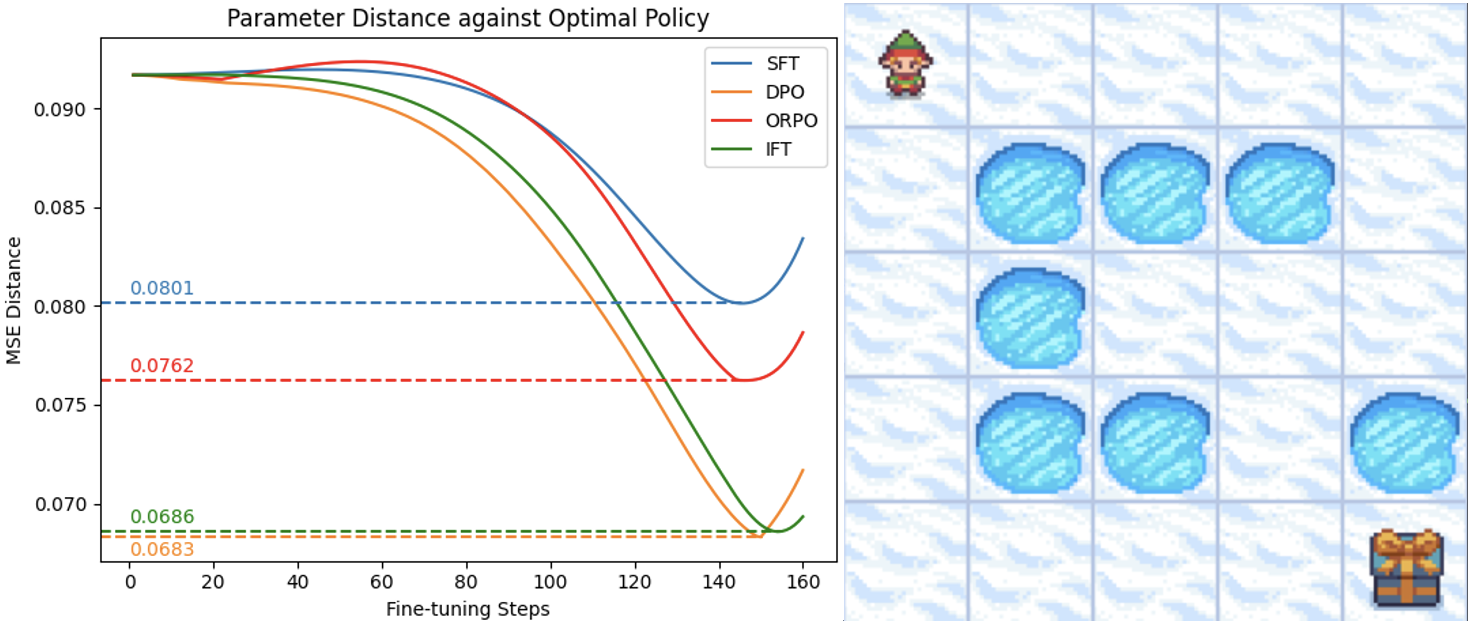
Figure 3: The Frozen Lake Game. Considering the MSE distance of parameters between the trained and optimal policy, IFT performs much better than SFT and ORPO, but slightly worse than DPO.

As scores on Open-LLM Leaderboard only partially reflect models’ performance, and GPT-4 inadequately models human language generation, further comparison to a truly optimal policy is necessary. Given the difficulty of obtaining an optimal policy representing human language, we validate our algorithm in a simplified setting called Frozen Lake frozenlake . In this environment, an agent attempts to find a gift on a nearly frozen lake with several holes, terminating the game upon finding the gift or falling into a hole. The limited number of states and actions in this game allows the optimal policy to be easily derived using classical RL methods.

To simulate parameterized policy alignment, we employ a two-layer fully connected neural network and design the environment with one optimal and one sub-optimal trajectory. The optimal parameterized policy is trained using the previously obtained optimal state-action probabilities, and various fine-tuning methods from LMs are compared. We evaluate performance by measuring the MSE distance between the optimal and trained policy parameters.

In this setting, IFT achieves a significantly better policy than SFT and ORPO, although it performs slightly worse than DPO. This is partly because, in terms of comparing how closely the explored grid aligns with the agent’s preference, the order is DPO > IFT > ORPO > SFT. Although ORPO also considers the negative trajectories sampled from policy, its direct incorporation of SFT loss with a fusion coefficient deviates its preference estimation, partially diminishing its effectiveness. Additionally, DPO, ORPO and IFT explore more grids than SFT, which helps the agent develop a better understanding of the environment.

6 Conclusion

In this paper, we first interpret SFT and some typical Preference Optimization methods into a unified framework using Preference Estimation and Transition Optimization. We then introduce an efficient and effective method called Intuitive Fine-Tuning (IFT), which achieves alignment directly from the base model using non-preference-labeled data. Finally, experiments on widely used benchmarks in NLP setting and in Frozen Lake environment demonstrate the competitive performance of IFT.

Limitations and Future Work. Our validation of IFT is limited to the fine-tuning stage, where data volume is constrained, leaving the scalability of IFT unexplored. Additionally, we primarily use Mistral-7B for baseline testing, and the generalization of IFT to larger and more diverse models requires exploration in the future.

Appendix A Theoretical Details

A.1 MDP In LMs

$\mathcal{M}=(S,A,\mathcal{T},r,\rho_{0})$:

• $A$, the concrete action space, consisting of $N_{A}$ vocabularies as defined by the tokenizer.

• $S$, the concrete state space, comprising $N_{S}=(N_{A})^{N}$ elements related to sequence length $N$. Each state represents a ordered permutation of vocabularies.

• $\rho_{0}$, the initial state of each generation, typically refers to the given instruction;

• $\mathcal{T}\in R^{N_{S}\times N_{A}}$, the state-action transition matrix of a given policy, indicating the probability of generating each token given different states;

• $r$, the reward assigned to a particular state-action pair.

A.2 Loss Function of IFT

Let’s begin by considering only one sampled state $s_{n}^{*}$ constrained by $\rho_{0}$,

Given the assumption of $T^{*}(s_{n}^{*},\rho_{0})=T^{*}(s_{N}^{*},\rho_{0})=1$, we have:

$$\mathcal{L}(\hat{T_{\theta}}(s_{n}^{*},\rho_{0})) =\log\frac{\hat{T_{\theta}}(s_{n}^{*},\rho_{0})}{T^{*}(s_{n}^{*},\rho_{0})}$$ (24)

$$=\log\frac{\hat{T_{\theta}}(s_{n}^{*},\rho_{0})}{T^{*}(s_{N}^{*},\rho_{0})}$$

$$=\log\frac{1}{\hat{T_{\theta}}(s_{N}^{*},s_{n}^{*})}$$

$$=-\log\prod\limits_{i=n}^{N}\mathcal{T}_{\theta}(a_{i}^{*},\delta_{\theta}(s_{i}^{*}))$$

$$=-\sum\limits_{i=n}^{N}\log\mathcal{T}_{\theta}(a_{i}^{*},\delta_{\theta}(s_{i}^{*}))$$

Next, we extend this to entire trajectories and the entire dataset to obtain the expected loss:

$$\mathcal{L}_{\text{IFT}}(\mathcal{T}_{\theta},\delta_{\theta}) =\mathbb{E}_{\rho_{0}\sim\mathcal{D}}\mathbb{E}_{s_{n}^{*}\sim\mathcal{S}_{\rho_{0}}^{*}}\left[\sum\limits_{n=0}^{N}\mathcal{L}\big{(}\hat{T_{\theta}}(s_{n}^{*},\rho_{0})\big{)}\right]$$ (25)

$$=\mathbb{E}_{\rho_{0}\sim\mathcal{D}}\mathbb{E}_{s_{i}^{*}\sim\mathcal{S}_{\rho_{0}}^{*}}\left[-\sum\limits_{n=0}^{N}\sum\limits_{i=n}^{N}\log\mathcal{T}_{\theta}(a_{i}^{*},\delta_{\theta}(s_{i}^{*}))\right]$$

where $s_{0}^{*}=\rho_{0}$, and $\mathcal{S}_{\rho_{0}}^{*}$ is the optimal $\rho_{0}$-constrained state space.

A.3 Proof for Bellman Equation

Considering only one sampled state $s_{n}^{*}$ constrained by $\rho_{0}$ in the datasets, we have:

$$\exp\big{(}-\mathcal{L}(\hat{T_{\theta}}(s_{n}^{*},\rho_{0}))\big{)} =\mathcal{T}_{\theta}(a_{n}^{*},\delta_{\theta}(s_{n}^{*}))\bigg{(}\sum\limits_{n+1}^{N}\mathcal{T}_{\theta}(a_{i}^{*},\delta_{\theta}(s_{i}^{*}))\bigg{)}$$ (26)

$$=\max\limits_{a}\bigg{[}\mathcal{T}_{\theta}(a,s_{n}^{*})\big{(}r+\gamma V(\hat{s^{\theta}_{n+1}})\big{)}\bigg{]}$$

$$=V_{\theta}(\hat{s_{n}^{\theta}})$$

where $r=(1-\gamma)V(\hat{s^{\theta}_{n+1}})$. This reward function implicitly accounts for the influence of the current prediction on future generations.

A.4 Reformulation of Typical Methods

We reformulate the loss function of some methods using the disparities of transition matrices as:

SFT

$$\mathcal{L}_{\text{SFT}}=\mathbb{E}_{\rho_{0}\sim\mathcal{D}}\mathbb{E}_{s_{i}^{*}\sim\mathcal{S}_{\rho_{0}}^{*}}\left[-\sum\limits_{i=0}^{N}\log\mathcal{T}_{\theta}(\pi^{*}(s_{i}^{*}),s_{i}^{*})\right]$$ (27)

where the human’s preference is unbiasedly estimated, but the model’s preference is inaccurately represented by using $s_{i}^{*}$.

PPO

$$\mathcal{L}_{\text{PPO}}=\mathbb{E}_{\rho_{0}\sim\mathcal{D}}\mathbb{E}_{s_{i}^{*}\sim\mathcal{S}_{\rho_{0}}^{*}}\left[-\sum\limits_{i=0}^{N}\mathcal{R}(\pi_{\theta}(s_{i}^{\theta}),s_{i}^{\theta})\right]$$ (28)

where $\mathcal{R}\in(-\infty,0]$ denotes the degree of closeness between human preferences and the state-action pairs chosen by model. The reward and loss will be zero only if the state-action pairs perfectly align with human preferences. Thus, PPO implicitly models the human policy $\pi^{*}$ through reward modeling, which can be formulated as follows:

$$\mathcal{R}=\pi_{\mathcal{R}}\leftarrow\min\limits_{\pi}\mathcal{L_{R}}$$ (29)

$$\mathcal{L_{R}}=\mathbb{E}_{\rho_{0}\sim\mathcal{D}}\mathbb{E}_{s_{i}^{+}\sim\mathcal{S}_{\rho_{0}}^{+},s_{i}^{-}\sim\mathcal{S}_{\rho_{0}}^{-}}\left[-\log\sigma\bigg{(}\sum\limits_{i=0}^{N}\log\mathcal{T_{R}}(\pi^{+}(s_{i}^{+})|s_{i}^{+})-\sum\limits_{i=0}^{N}\log\mathcal{T_{R}}(\pi^{-}(s_{i}^{-})|s_{i}^{-})\bigg{)}\right]$$ (30)

DPO-Online

$$\mathcal{L}_{\text{DPO}}=\mathbb{E}_{\rho_{0}\sim\mathcal{D}}\mathbb{E}_{s_{i}^{*}\sim\mathcal{S}_{\rho_{0}}^{*},s_{i}^{\theta}\sim\mathcal{S}_{\rho_{0}}^{\theta}}\left[-\log\sigma\bigg{(}\sum\limits_{i=0}^{N}\log\mathcal{T}_{\theta}(\pi^{*}(s_{i}^{*}),s_{i}^{*})-\sum\limits_{i=0}^{N}\log\mathcal{T}_{\theta}(\pi_{\theta}(s_{i}^{\theta}),s_{i}^{\theta})\bigg{)}\right]$$ (31)

Ideally, this loss function increases the probabilities of state-action pairs preferred by humans and decreases the probabilities of those chosen by the model. It unbiasedly estimate both the human’s and model’s preference.

DPO-Offline

$$\mathcal{L}_{\text{DPO}}=\mathbb{E}_{\rho_{0}\sim\mathcal{D}}\mathbb{E}_{s_{i}^{+}\sim\mathcal{S}_{\rho_{0}}^{+},s_{i}^{-}\sim\mathcal{S}_{\rho_{0}}^{-}}\left[-\log\sigma\bigg{(}\sum\limits_{i=0}^{N}\log\mathcal{T}_{\theta}(\pi^{+}(s_{i}^{+}),s_{i}^{+})-\sum\limits_{i=0}^{N}\log\mathcal{T}_{\theta}(\pi^{-}(s_{i}^{-}),s_{i}^{-})\bigg{)}\right]$$ (32)

In the offline circumstance, the positive samples can still represent the human preference correctly, as $s^{+}$ is usually similar to $s^{*}$. However, this is not the case for negative samples.As training progresses, $s^{-}$ becomes more and more out-of-distributions compared to the model’s preferred state $s^{\theta}$, leading to biased estimations.

IFT

$$\mathcal{L}_{\text{IFT}}=\mathbb{E}_{\rho_{0}\sim\mathcal{D}}\mathbb{E}_{s_{i}^{*}\sim\mathcal{S}_{\rho_{0}}^{*}}\left[-\sum\limits_{n=0}^{N}\sum\limits_{i=n}^{N}\log\mathcal{T}_{\theta}(a_{i}^{*},\delta_{\theta}(s_{i}^{*}))\right]$$ (33)

$$\delta_{\theta}(s_{i}^{*})=(1-\lambda)s_{i}^{*}+\lambda\pi_{\theta}(s_{i-1}^{*})$$ (34)

By using a model-based disturbance function, IFT constructs a residual connection in the temporal dimension, providing a better estimation for the model than SFT. Through this approach, IFT implicitly implements a Relation Propagation in the Transition Optimization stage, which considers the influence of current predictions on future outcomes. This propagation also reduces the influence of bias introduced by inaccurate estimations in earlier positions.

Appendix B Implementation Details

B.1 NLP Settings

For the coefficient $\beta$ in DPO and ORPO, we use 0.1 and 0.25 respectively, as presented in their original papers. For IFT, we choose 0.2 for $\lambda$ and incorporate a decay factor of 0.95 to fitting better with the Bellman Equation. We save checkpoints every 20k steps and select the results from the checkpoint with the best average score to demonstrate the performance of each method.

Table 4: Hyper-Parameters in NLP Setting

Name	Value
epoch	3
mini batch size	8
gradient accumulation step	64
warmup ratio	0.1
scheduler	cosine
learning rate	5e-7
optimizer	RMSprop
precision	bfloat16

We implement our main experiments on four NVIDIA A6000 GPUs. When using 60k single-target data, the entire training process for SFT and IFT takes approximately 20 hours, with each epoch lasting 7 hours. When using 60k pair-wise data, the training process for DPO and ORPO takes around 40 hours and 30 hours respectively, due to the differences in requirements for a reference model.

B.2 Frozen Lake Setting

We keep the similar hyper-parameters as in NLP setting for Frozen Lake game, running this environment on CPUs. Since our designed environment includes an optimal and a sub-optimal trajectory, we select the optimal trajectory as the target for SFT and IFT. For DPO and ORPO, the optimal and sub-optimal trajectories are used as positive and negative samples, respectively.

B.3 Pseudo-code of IFT

Algorithm 1 Intuitive Fine-Tuning

1:  Input:     Initial instruction $\rho_{0}$     Ground truth answer $s^{*}$ with $N$ tokens, $s^{*}[1],\ldots,s^{*}[N]$   

2:  Step 1: Inference One Step Ahead

3:  for $t$ in $[1,N]$ do

4:     Predict the probability distribution of the $t$-th token: $P_{t}^{\prime}=\mathcal{\pi_{\theta}}(s^{*}[0:t-1])$

5:     Sample the predicted token: $s^{\theta}[t]=\arg\max P_{t}^{\prime}$

6:  end for  

7:  Step 2: Intuitive Preference Estimation

8:  Encode $s^{*}$ and $s^{\theta}$ using the Embedding Layer $E$

9:  Compute the fused embedding $e=(1-\lambda)E(s^{*})+\lambda E(s^{\theta})$

10:  for $t$ in $[1,N]$ do

11:     Predict the probability distribution of the $t$-th token: $P_{t}^{\prime\prime}=(\mathcal{\pi_{\theta}}/E)(e[0:t-1])$

12:     Compute the token-level loss: $\mathcal{L}_{t}=\log(P_{t}^{\prime\prime},s^{*}[t])$

13:  end for  

14:  Step 3: Dynamic Relation Propagation

15:  for $t$ in $[1,N]$ do

16:     Compute the cumsum weight similar to Bellman Equation: $w_{t}=\sum\limits_{i=t}^{N}\alpha^{N-t}\mathcal{L}_{i}$

17:  end for  

18:  Output: Final loss $\mathcal{L}_{\text{IFT}}=w\cdot\mathcal{L}$

⬇

1def get_batch_logps(logits,

2 labels):

3

4 labels = labels[:, 1:].clone()

5 logits = logits[:, :-1, :]

6 loss_mask = (labels != -100)

7

8 labels[labels == -100] = 0

9

10 per_token_logps = torch.gather(logits.log_softmax(-1),

11 dim=2,

12 index=labels.unsqueeze(2)

13 ).squeeze(2)

14

15 return per_token_logps * loss_mask

⬇

1def get_ift_loss(policy,

2 input_ids,

3 attention_mask,

4 labels,

5 _lambda: float=0.2,

6 propagation_decay: float=0.95):

7

8 from torch_discounted_cumsum import discounted_cumsum_right

9 loss_mask = (labels[:, 1:] != -100)

10

11 # Step 1: Inference One Step Ahead

12 inputs_embeds = policy.embed_tokens(input_ids)

13 with torch.no_grad():

14 logits = policy(inputs_embeds=inputs_embeds,

15 attention_mask=attention_mask).logits

16 logps = get_batch_logps(logits, labels)

17

18 tokens_further = torch.cat((input_ids[:, 0].unsqueeze(-1),

19 torch.argmax(logits, dim=-1)[:, :-1]),

20 dim=-1)

21 input_ids_further = torch.where(labels==-100,

22 input_ids,

23 tokens_further)

24 attention_mask_further = attention_mask

25

26 # Step 2: Intuitive Preference Estimation

27 inputs_embeds_further = self.embed_tokens(input_ids_further)

28 inputs_embeds_further = (1 - _lambda) * inputs_embeds \

29 + _lambda * inputs_embeds_further

30 logits_further = policy(inputs_embeds=inputs_embeds_further,

31 attention_mask=attention_mask_further,

32 ).logits

33 logps_further = _get_batch_logps(logits_further, labels)

34 loss_orig = -logps / loss_mask.sum(-1).unsqueeze(-1)

35

36 # Step 3: Dynamic Relation Propagation

37 cumsum_weight = discounted_cumsum_right(loss_orig,

38 gamma=propagation_decay)

39 cumsum_weight[loss_mask == 0] = 0

40 cumsum_weight *= (loss_mask.sum(-1, keepdim=True) \

41 / cumsum_weight.sum(-1, keepdim=True))

42

43 loss_ift = (-logps * cumsum_weight).sum(-1) / loss_mask.sum(-1)

44

45 return loss_ift.mean()

References

- [1] Josh Achiam, Steven Adler, Sandhini Agarwal, Lama Ahmad, Ilge Akkaya, Florencia Leoni Aleman, Diogo Almeida, Janko Altenschmidt, Sam Altman, Shyamal Anadkat, et al. Gpt-4 technical report. arXiv preprint arXiv:2303.08774, 2023.
- [2] Hritik Bansal, Ashima Suvarna, Gantavya Bhatt, Nanyun Peng, Kai-Wei Chang, and Aditya Grover. Comparing bad apples to good oranges: Aligning large language models via joint preference optimization. arXiv preprint arXiv:2404.00530, 2024.
- [3] Emily M Bender, Timnit Gebru, Angelina McMillan-Major, and Shmargaret Shmitchell. On the dangers of stochastic parrots: Can language models be too big? In Proceedings of the 2021 ACM conference on fairness, accountability, and transparency, pages 610–623, 2021.
- [4] Rishi Bommasani, Drew A Hudson, Ehsan Adeli, Russ Altman, Simran Arora, Sydney von Arx, Michael S Bernstein, Jeannette Bohg, Antoine Bosselut, Emma Brunskill, et al. On the opportunities and risks of foundation models. arXiv preprint arXiv:2108.07258, 2021.
- [5] Ralph Allan Bradley and Milton E Terry. Rank analysis of incomplete block designs: I. the method of paired comparisons. Biometrika, 39(3/4):324–345, 1952.
- [6] Tom Brown, Benjamin Mann, Nick Ryder, Melanie Subbiah, Jared D Kaplan, Prafulla Dhariwal, Arvind Neelakantan, Pranav Shyam, Girish Sastry, Amanda Askell, et al. Language models are few-shot learners. Advances in neural information processing systems, 33:1877–1901, 2020.
- [7] Daniele Calandriello, Daniel Guo, Remi Munos, Mark Rowland, Yunhao Tang, Bernardo Avila Pires, Pierre Harvey Richemond, Charline Le Lan, Michal Valko, Tianqi Liu, et al. Human alignment of large language models through online preference optimisation. arXiv preprint arXiv:2403.08635, 2024.
- [8] Zixiang Chen, Yihe Deng, Huizhuo Yuan, Kaixuan Ji, and Quanquan Gu. Self-play fine-tuning converts weak language models to strong language models. arXiv preprint arXiv:2401.01335, 2024.
- [9] Hyung Won Chung, Le Hou, Shayne Longpre, Barret Zoph, Yi Tay, William Fedus, Yunxuan Li, Xuezhi Wang, Mostafa Dehghani, Siddhartha Brahma, et al. Scaling instruction-finetuned language models. Journal of Machine Learning Research, 25(70):1–53, 2024.
- [10] Peter Clark, Isaac Cowhey, Oren Etzioni, Tushar Khot, Ashish Sabharwal, Carissa Schoenick, and Oyvind Tafjord. Think you have solved question answering? try arc, the ai2 reasoning challenge. arXiv preprint arXiv:1803.05457, 2018.
- [11] Karl Cobbe, Vineet Kosaraju, Mohammad Bavarian, Mark Chen, Heewoo Jun, Lukasz Kaiser, Matthias Plappert, Jerry Tworek, Jacob Hilton, Reiichiro Nakano, et al. Training verifiers to solve math word problems. arXiv preprint arXiv:2110.14168, 2021.
- [12] Ganqu Cui, Lifan Yuan, Ning Ding, Guanming Yao, Wei Zhu, Yuan Ni, Guotong Xie, Zhiyuan Liu, and Maosong Sun. Ultrafeedback: Boosting language models with high-quality feedback. arXiv preprint arXiv:2310.01377, 2023.
- [13] Ning Ding, Yulin Chen, Bokai Xu, Yujia Qin, Zhi Zheng, Shengding Hu, Zhiyuan Liu, Maosong Sun, and Bowen Zhou. Enhancing chat language models by scaling high-quality instructional conversations. arXiv preprint arXiv:2305.14233, 2023.
- [14] Hanze Dong, Wei Xiong, Deepanshu Goyal, Yihan Zhang, Winnie Chow, Rui Pan, Shizhe Diao, Jipeng Zhang, Kashun Shum, and Tong Zhang. Raft: Reward ranked finetuning for generative foundation model alignment. arXiv preprint arXiv:2304.06767, 2023.
- [15] Yann Dubois, Chen Xuechen Li, Rohan Taori, Tianyi Zhang, Ishaan Gulrajani, Jimmy Ba, Carlos Guestrin, Percy S Liang, and Tatsunori B Hashimoto. Alpacafarm: A simulation framework for methods that learn from human feedback. Advances in Neural Information Processing Systems, 36, 2024.
- [16] Kawin Ethayarajh, Winnie Xu, Niklas Muennighoff, Dan Jurafsky, and Douwe Kiela. Kto: Model alignment as prospect theoretic optimization. arXiv preprint arXiv:2402.01306, 2024.
- [17] Farama. Frozen lake. https://gymnasium.farama.org/environments/toy_text/frozen_lake/, 2023. Accessed: 2024-05-19.
- [18] Yang Guan, Shengbo Eben Li, Jingliang Duan, Jie Li, Yangang Ren, Qi Sun, and Bo Cheng. Direct and indirect reinforcement learning. International Journal of Intelligent Systems, 36(8):4439–4467, 2021.
- [19] Shangmin Guo, Biao Zhang, Tianlin Liu, Tianqi Liu, Misha Khalman, Felipe Llinares, Alexandre Rame, Thomas Mesnard, Yao Zhao, Bilal Piot, et al. Direct language model alignment from online ai feedback. arXiv preprint arXiv:2402.04792, 2024.
- [20] Yiju Guo, Ganqu Cui, Lifan Yuan, Ning Ding, Jiexin Wang, Huimin Chen, Bowen Sun, Ruobing Xie, Jie Zhou, Yankai Lin, et al. Controllable preference optimization: Toward controllable multi-objective alignment. arXiv preprint arXiv:2402.19085, 2024.
- [21] Jiwoo Hong, Noah Lee, and James Thorne. Reference-free monolithic preference optimization with odds ratio. arXiv preprint arXiv:2403.07691, 2024.
- [22] Albert Q Jiang, Alexandre Sablayrolles, Arthur Mensch, Chris Bamford, Devendra Singh Chaplot, Diego de las Casas, Florian Bressand, Gianna Lengyel, Guillaume Lample, Lucile Saulnier, et al. Mistral 7b. arXiv preprint arXiv:2310.06825, 2023.
- [23] Saeed Khaki, JinJin Li, Lan Ma, Liu Yang, and Prathap Ramachandra. Rs-dpo: A hybrid rejection sampling and direct preference optimization method for alignment of large language models. arXiv preprint arXiv:2402.10038, 2024.
- [24] Alessandro Lazaric, Marcello Restelli, and Andrea Bonarini. Reinforcement learning in continuous action spaces through sequential monte carlo methods. Advances in neural information processing systems, 20, 2007.
- [25] Harrison Lee, Samrat Phatale, Hassan Mansoor, Kellie Lu, Thomas Mesnard, Colton Bishop, Victor Carbune, and Abhinav Rastogi. Rlaif: Scaling reinforcement learning from human feedback with ai feedback. arXiv preprint arXiv:2309.00267, 2023.
- [26] Sergey Levine, Peter Pastor, Alex Krizhevsky, Julian Ibarz, and Deirdre Quillen. Learning hand-eye coordination for robotic grasping with deep learning and large-scale data collection. The International journal of robotics research, 37(4-5):421–436, 2018.
- [27] Bo Li, Peng Qi, Bo Liu, Shuai Di, Jingen Liu, Jiquan Pei, Jinfeng Yi, and Bowen Zhou. Trustworthy ai: From principles to practices. ACM Comput. Surv., aug 2022. Just Accepted.
- [28] Stephanie Lin, Jacob Hilton, and Owain Evans. Truthfulqa: Measuring how models mimic human falsehoods. arXiv preprint arXiv:2109.07958, 2021.
- [29] Tianqi Liu, Yao Zhao, Rishabh Joshi, Misha Khalman, Mohammad Saleh, Peter J Liu, and Jialu Liu. Statistical rejection sampling improves preference optimization. arXiv preprint arXiv:2309.06657, 2023.
- [30] Wei Liu, Weihao Zeng, Keqing He, Yong Jiang, and Junxian He. What makes good data for alignment? a comprehensive study of automatic data selection in instruction tuning. arXiv preprint arXiv:2312.15685, 2023.
- [31] Xiao Liu, Xixuan Song, Yuxiao Dong, and Jie Tang. Extensive self-contrast enables feedback-free language model alignment. arXiv preprint arXiv:2404.00604, 2024.
- [32] Arindam Mitra, Hamed Khanpour, Corby Rosset, and Ahmed Awadallah. Orca-math: Unlocking the potential of slms in grade school math. arXiv preprint arXiv:2402.14830, 2024.
- [33] Long Ouyang, Jeffrey Wu, Xu Jiang, Diogo Almeida, Carroll Wainwright, Pamela Mishkin, Chong Zhang, Sandhini Agarwal, Katarina Slama, Alex Ray, et al. Training language models to follow instructions with human feedback. Advances in neural information processing systems, 35:27730–27744, 2022.
- [34] Benjamin Plaut, Khanh Nguyen, and Tu Trinh. Softmax probabilities (mostly) predict large language model correctness on multiple-choice q&a. arXiv preprint arXiv:2402.13213, 2024.
- [35] Rafael Rafailov, Archit Sharma, Eric Mitchell, Christopher D Manning, Stefano Ermon, and Chelsea Finn. Direct preference optimization: Your language model is secretly a reward model. Advances in Neural Information Processing Systems, 36, 2024.
- [36] Keisuke Sakaguchi, Ronan Le Bras, Chandra Bhagavatula, and Yejin Choi. Winogrande: An adversarial winograd schema challenge at scale. Communications of the ACM, 64(9):99–106, 2021.
- [37] John Schulman, Filip Wolski, Prafulla Dhariwal, Alec Radford, and Oleg Klimov. Proximal policy optimization algorithms. arXiv preprint arXiv:1707.06347, 2017.
- [38] Harm Seijen and Rich Sutton. True online td (lambda). In International Conference on Machine Learning, pages 692–700. PMLR, 2014.
- [39] Richard S Sutton. Learning to predict by the methods of temporal differences. Machine learning, 3:9–44, 1988.
- [40] Fahim Tajwar, Anikait Singh, Archit Sharma, Rafael Rafailov, Jeff Schneider, Tengyang Xie, Stefano Ermon, Chelsea Finn, and Aviral Kumar. Preference fine-tuning of llms should leverage suboptimal, on-policy data. arXiv preprint arXiv:2404.14367, 2024.
- [41] Polina Tsvilodub, Hening Wang, Sharon Grosch, and Michael Franke. Predictions from language models for multiple-choice tasks are not robust under variation of scoring methods. arXiv preprint arXiv:2403.00998, 2024.
- [42] Lewis Tunstall, Edward Beeching, Nathan Lambert, Nazneen Rajani, Kashif Rasul, Younes Belkada, Shengyi Huang, Leandro von Werra, Clémentine Fourrier, Nathan Habib, et al. Zephyr: Direct distillation of lm alignment. arXiv preprint arXiv:2310.16944, 2023.
- [43] Oriol Vinyals, Igor Babuschkin, Wojciech M Czarnecki, Michaël Mathieu, Andrew Dudzik, Junyoung Chung, David H Choi, Richard Powell, Timo Ewalds, Petko Georgiev, et al. Grandmaster level in starcraft ii using multi-agent reinforcement learning. Nature, 575(7782):350–354, 2019.
- [44] Sean Welleck, Ilia Kulikov, Stephen Roller, Emily Dinan, Kyunghyun Cho, and Jason Weston. Neural text generation with unlikelihood training. arXiv preprint arXiv:1908.04319, 2019.
- [45] Wei Xiong, Hanze Dong, Chenlu Ye, Ziqi Wang, Han Zhong, Heng Ji, Nan Jiang, and Tong Zhang. Iterative preference learning from human feedback: Bridging theory and practice for rlhf under kl-constraint. In ICLR 2024 Workshop on Mathematical and Empirical Understanding of Foundation Models, 2023.
- [46] Yueqin Yin, Zhendong Wang, Yi Gu, Hai Huang, Weizhu Chen, and Mingyuan Zhou. Relative preference optimization: Enhancing llm alignment through contrasting responses across identical and diverse prompts. arXiv preprint arXiv:2402.10958, 2024.
- [47] Weizhe Yuan, Richard Yuanzhe Pang, Kyunghyun Cho, Sainbayar Sukhbaatar, Jing Xu, and Jason Weston. Self-rewarding language models. arXiv preprint arXiv:2401.10020, 2024.
- [48] Zheng Yuan, Hongyi Yuan, Chuanqi Tan, Wei Wang, Songfang Huang, and Fei Huang. Rrhf: Rank responses to align language models with human feedback without tears. arXiv preprint arXiv:2304.05302, 2023.
- [49] Ruiqi Zhang, Licong Lin, Yu Bai, and Song Mei. Negative preference optimization: From catastrophic collapse to effective unlearning. arXiv preprint arXiv:2404.05868, 2024.
- [50] Yao Zhao, Rishabh Joshi, Tianqi Liu, Misha Khalman, Mohammad Saleh, and Peter J Liu. Slic-hf: Sequence likelihood calibration with human feedback. arXiv preprint arXiv:2305.10425, 2023.
- [51] Chujie Zheng, Hao Zhou, Fandong Meng, Jie Zhou, and Minlie Huang. Large language models are not robust multiple choice selectors. In The Twelfth International Conference on Learning Representations, 2023.
- [52] Bowen Zhou and Ning Ding. Generative ai for complex scenarios: Language models are sequence processors. International Journal of Artificial Intelligence and Robotics Research, 2024.
- [53] Daniel M Ziegler, Nisan Stiennon, Jeffrey Wu, Tom B Brown, Alec Radford, Dario Amodei, Paul Christiano, and Geoffrey Irving. Fine-tuning language models from human preferences. arXiv preprint arXiv:1909.08593, 2019.