An Investigation into the Thermoelectric Characteristics of Silver-based Chalcopyrites Utilizing a Non-empirical Range-separated Dielectric-dependent Hybrid Approach

Abstract

Our investigation explores the intricate domain of thermoelectric phenomena within silver (Ag)-infused chalcopyrites, focusing on compositions such as AgXTe₂ (where X=Ga, In) and the complex quaternary system Ag₂ZnSn/GeY₂ (with Y=S, Se). Using a sophisticated combination of methodologies, we integrate a non-empirical screened dielectric-dependent hybrid (DDH) functional with semiclassical Boltzmann transport theory. This approach allows us to conduct a detailed analysis of critical thermoelectric properties, including electrical conductivity, Seebeck coefficient, and power factor. Our methodology goes beyond superficial assessments, delving into the intricate interplay of material properties to reveal their true thermoelectric potential. Additionally, we investigate the often-overlooked phenomena of phonon scattering by leveraging both the elastic constant tensor and the deformation potential method. This enables a rigorous examination of electron relaxation time and lattice thermal conductivity, enhancing the robustness of our predictions and demonstrating our commitment to thorough exploration.Through our rigorous investigation, we identify materials with a thermoelectric figure of merit (ZT = $\sigma S^{2}T/\kappa$) exceeding the critical threshold of unity. This significant achievement signals the discovery of materials capable of revolutionizing efficient thermoelectric systems. Our findings delineate a promising trajectory, laying the groundwork for the emergence of a new class of Ag-based chalcopyrites distinguished by their exceptional thermoelectric characteristics. This research not only contributes to the understanding of materials science principles but also catalyzes transformative advancements in thermoelectric technology.

I Introduction

Thermoelectric (TE) materials have captured significant interest, particularly in the last two decades, for their unique ability to directly convert heat into electricity without relying on moving components DiSalvo (1999); Bell (2008). Positioned as crucial contributors to the evolution of a more sustainable global energy landscape, TE materials offer promising applications, including onboard power for wearable electronic sensors and systems designed for disaster mitigation Leonov and Vullers (2009); Boyer and Cisse (1992); Lv et al. (2022). Despite these possibilities, the practical deployment of TE devices has faced challenges, primarily due to their typically modest energy conversion efficiency. The efficiency of TE materials is assessed through their dimensionless figure-of-merit ZT =$\sigma S^{2}T/\kappa$, a key parameter influencing their overall efficiency. The expression for the dimensionless figure-of-merit (ZT) is defined as the product of the Seebeck coefficient (S), electrical conductivity ($\sigma$), and absolute temperature (T), divided by the total thermal conductivity ($\kappa$), which encompasses both electronic and lattice contributions. The pursuit of identifying thermoelectric (TE) materials with elevated ZT values has been a central focus of research in this field for several decades Mahan and Sofo (1996); Heremans et al. (2008).

In thermoelectric cooling devices designed for commercial applications, Bi2Te3 stands out as a commonly employed thermoelectric (TE) material Hong et al. (2018), while PbTe is favored for high-temperature TE applications Gelbstein et al. (2005). Exploration into materials such as NiTiSn and ZrNiSn is ongoing Downie et al. (2014), driven by their potential in thermoelectric applications. Their remarkable performance can be attributed to the value of ZT near to 1. The efficacy of these materials is primarily influenced by the increased power factor ($\sigma S^{2}T$) or the reduction in thermal conductivity. Owing to the toxic nature of lead-based PbTe and the high cost associated with Tellurium, the production of these thermoelectric (TE) materials is constrained.

In recent years, the spotlight in thermoelectrics has shifted towards Ag-based chalcopyrites, drawing considerable attention. This increased focus is credited to their exceptional adaptability in crystal structures and electronic band arrangements, as noted in prior research Cao et al. (2020); Parker and Singh (2012). Diamond-like compounds, encompassing ternary and quaternary Ag-based chalcopyrites such as AgXY₂ (X=Ga, In and Y=S, Se, Te) and Ag₂PQR₄ (P=Mg, Mn, Fe, Zn, Cd, Hg; Q= Si, Ge, Sn; R= S, Se, Te), have become a focal point due to their versatile composition and functional adjustability. These attributes position them as promising contenders for applications in thermoelectric devices.

Recent investigations have revealed that AgGaTe₂ and AgInTe₂ boast thermal conductivities of 1.94 and 2.05 W m^-1 K^-1, respectively, at standard room temperature, as documented by Charoenphakdee et al. Charoenphakdee et al. (2009). This underscores their potential as promising contenders in the realm of thermoelectric materials, given their notably low thermal conductivities. Sharma et al. Sharma et al. (2014) conducted an exhaustive analysis of AgGaTe₂’s thermal attributes, delving into its Debye temperature, entropy, and heat capacity under diverse pressure and temperature conditions. Understanding the intricate interplay among thermoelectric transport characteristics, temperature variations, and carrier concentration is paramount. Such understanding forms the bedrock for discerning the optimal doping carrier concentration, thus propelling further experimental exploration and the advancement of thermoelectric material applications. AgGaTe₂ emerges as a promising candidate for p-type doping in thermoelectric applications, with an optimal carrier concentration ranging from $10^{19}$ to $10^{20}$ cm^-3 Parker and Singh (2012); Peng et al. (2014). Predictions using the PBE+U approach Yang et al. (2017) indicate ZT values of 1.38 and 0.91 at 800 K, corresponding to carrier concentrations of $2.12\times 10^{20}$ cm^-3 and $1.97\times 10^{20}$ cm^-3 for p-type AgGaTe₂ (AGT) and AgInTe₂ (AIT), respectively.

Moving on to Ag₂ZnSnS₄ (AZTS) and Ag₂ZnSnSe₄ (AZTSe), experimental findings from Li et al. Li et al. (2013) and Kaya et al. Kaya et al. (2015) report band gaps of 1.20 eV and 1.40 eV, respectively, showcasing high absorption coefficients ideal for solar cell applications, as highlighted by Chagarov et al. Chagarov et al. (2016). Synthesis efforts led to an impressive 10.7$\%$ efficiency for AZTS Xianfeng et al. (2013). Beyond photovoltaics, AZTS has found utility in photocatalysts Li et al. (2013) and photo-electrochemical applications Yeh and Cheng (2014). Comparisons with Cu₂ZnSnS₄ (CZTS) reveal similar structural and phase stability but distinct conductivity characteristics, as elucidated by Chen et al. Chen et al. (2009) and Chagarov et al. Chagarov et al. (2016). Although no experimental studies have been conducted on Ag₂ZnGeS₄ (AZGS) and Ag₂ZnGeSe₄ (AZGSe), theoretical investigations by Nainaa et al. Nainaa et al. (2019) employing mbj-GGA exchange-correlation approximation suggest heightened absorption and carrier concentration compared to CZTS, suggesting promising prospects for improving solar cell performance.

Silver-based quaternary materials’ thermoelectric properties remain largely unexplored. Optimizing parameters like carrier concentration, effective mass, and band gap is essential for maximizing the figure of merit (ZT), as highlighted by Snyder et al. Snyder and Toberer (2008). This Paper employs the multiband Boltzmann transport equations (BTEs) as the analytical framework to delve into and prognosticate the thermoelectric (TE) transport characteristics. Essential parameters such as the band gap and effective mass pertinent to each band are meticulously derived through first-principles calculations, serving as pivotal inputs for solving the intricate BTEs. Furthermore, the relaxation time approximation (RTA), predicated upon the multiband carrier transport model elucidated in reference Zhou et al. (2010), is judiciously incorporated into the analysis. To showcase the efficacy and versatility of our proposed methodology, an exhaustive investigation is conducted on the TE properties of an array of materials including AGT, AIT, AZTS, AZTSe, AZGS, and AZGSe. Leveraging the insights garnered from these analyses, we meticulously delineate the optimal carrier concentrations conducive to achieving peak figure of merit (ZT) for the aforementioned materials. It is worth noting that this methodology can be seamlessly extended to explore the TE characteristics of various other Ag-based materials similarly, thus offering a comprehensive framework for advancing the understanding and design of high-performance thermoelectric materials Chung and Buessem (1967).

II Methodods and technical details

II.1 Method

All the calculations are performed using the density functional method within screened dielectric dependent hybrid (DDH) by solving a generalized Kohn-Sham (gKS) scheme having the following form of the screened xc potential,

$$V_{xc}^{DDH}(1,\epsilon_{\infty}^{-1};\mu) = [1-(1-\epsilon_{\infty}^{-1})Erf(\mu r)]V_{x}^{Fock}$$

$$- (1-\epsilon_{\infty}^{-1})V_{x}^{sl-sr,\mu}+(1-\epsilon_{\infty}^{-1})V_{x}^{sl}+V_{c}^{sl}~{}.$$

This is proposed in ref. Chen et al. (2018) named as a dielectric dependent ange-separated hybrid using Coulomb attenuation method (DD-RSH-CAM) or simply DDH (used throughout this paper). The key feature of this method is that it takes similarities of the static version of the $GW$, named COH-SEX, where Coulomb hole (COH) is taken care by the GGA approximates and screened exchange (SEX) by Fock term Cui et al. (2018).

For reliable DDH calculations of Eq. LABEL:hy-eq6, one has to determine the macroscopic static dielectric constant, $\epsilon_{\infty}$, and screening parameter, $\mu$. Although the PBE calculated $\epsilon_{\infty}$ often gives good results, self-consistent updating of $\epsilon_{\infty}$ using DDH is more reliable, especially when PBE predicts the system to be metallic instead of semiconductors Ghosh et al. (2024). The parameter $\mu$ can also be determined using several procedures. In particular, we consider the procedure proposed in ref. Jana et al. (2023), which is named as $\mu_{eff}^{fit}$ and obtained using the compressibility sum rule together with LR-TDDFT Jana et al. (2023).

II.2 Technical details of calculation procedures

To optimize the structure and calculate electronic properties of Ag-based thermoelectric (TE) materials, we utilize the Vienna Ab-initio Simulation Package (VASP) code Kresse and Furthmüller (1996a, b) within the Generalized Gradient Approximation in the Perdew-Burke-Ernzerhof (GGA-PBE) functional framework Perdew et al. (1996). These calculations are conducted using density-functional theory (DFT). Handling the complexities of Ag-d electrons poses a challenge, leading us to adopt the dielectric-dependent hybrid (DDH) approach Jana et al. (2023). This decision is driven by DDH’s notable enhancements in the band gaps of Chalcopyrites Ghosh et al. (2024), rendering it well-suited for addressing the unique characteristics of Ag-d electrons. This involves calculating the ion-clamped static (optical) dielectric constant, or electronic dielectric constant ($\epsilon_{\infty}$), and the screening parameter ($\mu$). We set a kinetic energy cutoff of $400$ eV for all Density Functional Theory (DFT) calculations. A Monkhorst-Pack (MP) $\Gamma$-centered $8\times 8\times 8$ k-points mesh is employed to sample the Brillouin Zone (BZ). Convergence of electronic energies is pursued until reaching a tolerance of $10^{-6}$ eV across all DFT methods to ensure self-consistency. Structural relaxation continues until Hellmann-Feynman forces on atoms diminish to below 0.01 eV/Å^-1. Throughout these computations, we rely on the VASP-recommended Projector-Augmented Wave (PAW) pseudopotentials Kresse and Joubert (1999); Woo et al. (1997). Incorporating spin-orbit coupling (SOC) in these calculations is crucial, given its notable impact on the effective mass tensor, even in materials with low atomic masses Silva et al. (2001). Elastic constants ($C_{ij}$) are derived from the strain-stress relationship, employing a 15% strain in the interval of 5. According to the Voigt-Reuss-Hill (VRH) theory in a macroscopic system Den Toonder et al. (1999), corresponding elastic properties such as bulk modulus $B$ and shear modulus $G$ can be evaluated from these constants. The VRH approach is deemed to be in good agreement with experimental measurements.

The primary focus of the screened DDH (Density Dependent Hybrid) approach is to determine the high-frequency macroscopic static dielectric constants. This involves calculating the ion-clamped static (optical) dielectric constant, or electronic dielectric constant ($\epsilon_{\infty}$), and the screening parameter ($\mu$). The steps for performing DDH self-consistent field (scf) calculations are as follows:

(1). Calculate $\mu_{eff}^{fit}$ as mentioned in Section  II.1 with LDA orbitals. (2). Start with $\epsilon_{\infty}(q\rightarrow 0,\omega\rightarrow 0)$ obtained from the PBE functional (RPA@PBE), and plug it into the DDH expression Eq. (6) along with the previously calculated $\mu_{eff}^{fit}$. (3). Perform the DDH calculation and update $\epsilon_{\infty}(q\rightarrow 0,\omega\rightarrow 0)$ using the result from RPA@DDH, iterating until self-consistency in $\epsilon_{\infty}(q\rightarrow 0,\omega\rightarrow 0)$ is reached.

The values of $\epsilon_{\infty}$ (RPA@PBE), $\epsilon_{\infty}$ (RPA@DDH), and $\mu_{eff}^{fit}$ obtained for our systems are shown in Table 1.

Table 1: The high-frequency macroscopic static dielectric constants, ion-clamped static (optical) dielectric constants, and electronic dielectric constants ($\epsilon_{\infty}$) for the PBE and DDH methods, along with screening parameters ($\mu$ in Å^-1), are key parameters under consideration.

	$\epsilon_{\infty}$ (RPA@PBE)	$\epsilon_{\infty}$ (RPA@DDH)	$\mu=\mu_{eff}^{fit}$
AGT	15.39	7.99	1.49
AIT	11.8	7.69	1.33
AZTS	17.6	5.37	1.43
AZTSe	11.85	6.38	1.36
AZGS	7.02	5.347	1.39
AZGSe	8.45	6.55	1.47

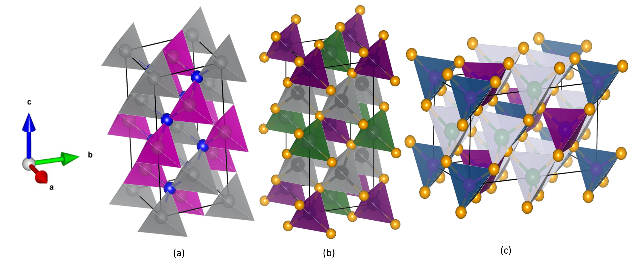
Figure 1: The PBE method was used to optimize the crystal structures of (a) tetragonal AXT (where X = Ga/In) with Te atoms depicted in blue, Ga/In atoms in pink, and Ag atoms in grey. (b) The crystal structure of AZTQ (where Q=S/Se) shows orange S/Se atoms, magenta Zn atoms, grey Ag atoms, and green Sn atoms. (c) In the structure of AZGQ (where Q=S/Se), orange S/Se atoms are bonded with blue Ge atoms, alongside magenta Zn atoms and silver Ag atoms.

Table 2: PBE optimized lattice constants ($a$, $c$), distortion parameter $\eta=c/2a$ used for DDH calculations and bond length of Ag atom with Te, S and Se for AXT (X = Ga, In), AZTY, and AZGY with (Y=S, Se) utilizing the DDH and Experiemntal methods (if available). Percent deviations from experimental data (where accessible) are presented in parentheses.

	$a$ (Å)		$c$ (Å)		$\eta$(Å)		$d_{Ag-y}$ (y=Te, S, Se)
	DDH	Exp.	DDH	Exp.	DDH	Exp.	DDH	Exp.
AGT	6.40	6.288	12.32	11.940	0.9625	0.949	2.799	2.76
	(1.78)		(3.1)		(1.4)		(1.41)
AIT	6.56	6.467	13.00	12.633	0.9908	0.977	2.811	2.78
	(1.43)		(2.9)		(1.41)		(1.07)
AZTS	5.562	5.693	12.15	11.342	1.092	0.996	2.561	2.57
	(2.30)		(7.12)		(9.63)		(-0.3)
AZTSe	5.873	5.99	12.606	11.47	1.07	0.960	2.656	2.65
	(1.95)		(9.76)		(11.45)		(-0.22)
AZGS	5.76	–	10.633	–	0.24	–	2.578	–
AZGSe	6.03	–	11.25	–	0.24	–	2.678	–

III Result and Discussion

III.1 Details of crystal Structure

Figure 1 illustrates the crystal structures of AXT (X=Ga/In) and stannite AZPQ (P=Sn/Ge and Q= S/Se), with $a$, $b$, and $c$ representing the lattice constants along the $x$, $y$, and $z$ directions, respectively. AXT is experimentally known to crystallize in tetragonal symmetry with space group $I{\bar{4}}2d$ Shaposhnikov et al. (2012), while AZSQ and AZGQ (where Q=S/Se) exhibits tetragonal symmetry with $I{\bar{4}}2m$ Wada (2022) and $I{\bar{4}}$ space groups. We optimized the lattice constants using PBE before proceeding with further calculations for TE properties. The PBE-optimized lattice constants ($a=b\neq c$) and tetragonal distortion ($\eta$), along with experimental values (when available), are summarized in Table 2. For GGA pseudopotentials, we selected the valence configurations of the constituent atoms as follows: Ag($4d^{10}5s^{1}$), Zn($3d^{10}4p^{2}$), Sn($4d^{10}5s^{2}5p^{2}$), S($3s^{2}3p^{4}$), Se($4s^{2}4p^{4}$), Ga($3d^{10}4s^{2}4p^{1}$), Ge($3d^{10}4s^{2}4p^{2}$), In($4d^{10}5s^{2}5p^{1}$), and Te($5s^{2}5p^{4}$). The different atomic radii of Ag element with chalcogens result in distinct bond formations, as shown in Table 2, contributing to reduced thermal conductivity due to the locally distorted environment formed by Te, S and Se. Figure 1 illustrates the crystal structures of AXT (X=Ga/In) and stannite AZPQ (P=Sn/Ge and Q= S/Se), with $a$, $b$, and $c$ representing the lattice constants along the $x$, $y$, and $z$ directions, respectively. AXT is experimentally known to crystallize in tetragonal symmetry with space group $I{\bar{4}}2d$ Shaposhnikov et al. (2012), while AZSQ and AZGQ (where Q=S/Se) exhibits tetragonal symmetry with $I{\bar{4}}2m$ Wada (2022) and $I{\bar{4}}$  Nainaa et al. (2019) space groups. We optimized the lattice constants using PBE before proceeding with further calculations for TE properties. The PBE-optimized lattice constants ($a=b\neq c$) and tetragonal distortion ($\eta$), along with experimental values (when available), are summarized in Table 2. For GGA pseudopotentials, we selected the valence configurations of the constituent atoms as follows: Ag($4d^{10}5s^{1}$), Zn($3d^{10}4p^{2}$), Sn($4d^{10}5s^{2}5p^{2}$), S($3s^{2}3p^{4}$), Se($4s^{2}4p^{4}$), Ga($3d^{10}4s^{2}4p^{1}$), Ge($3d^{10}4s^{2}4p^{2}$), In($4d^{10}5s^{2}5p^{1}$), and Te($5s^{2}5p^{4}$). The different atomic radii of these elements result in distinct bond formations, as shown in Table 2, contributing to reduced thermal conductivity due to the locally distorted environment formed by S/Se.

III.2 Band Structures

III.2.1 AXT

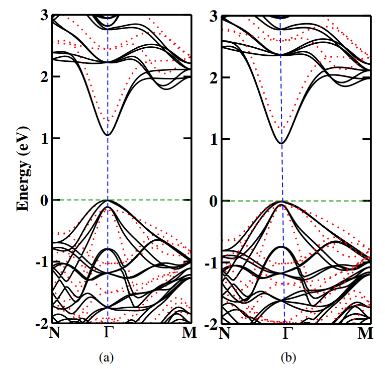
Figure 2: Computed band structure for (a) AGT and (b) AIT employing DDH, delineating bands without SOC via dashed red lines and with SOC via solid black lines.

We conducted computational investigations to determine the band gaps of AXT (X=Ga, In) and AZPQ (P=Ge/Sn and Q=S/Se) using density functional theory (DFT) with the Dielectric Dependent Hybrid (DDH) functional, while considering.

Our analysis confirmed direct band gaps at the $\Gamma$ point. Notably, we found that the band gaps calculated using the PBE functional significantly underestimated reported values by 80$\%$ to 100$\%$. In contrast, the DDH approach provided band gap values in close agreement with experimental data. Additionally, our calculations revealed that the inclusion of spin-orbit coupling (SOC) induced shifts in band positions, consistent with previous studies (Gong et al., 2015). Table 3 summarizes the band gap values obtained with and without SOC. The importance of band gap in determining thermoelectric properties is underscored by our analysis of the band structures of AgGaTe₂ and AgInTe₂, as depicted in Figures  2 (a) and (c), respectively. We observed significant variations in band gap values when considering SOC, highlighting its influence on electronic properties. Specifically, for AgGaTe₂, the band gap varied from 1.25 eV to 1.06 eV, and 1.17 eV to 0.94 eV with SOC. The pronounced coupling between Ag-d and Te-p atoms at the valence band maximum (VBM) played a crucial role in determining energy disparities between orbitals.

Furthermore, we noted that the substantial SOC originating from heavy Te atoms caused the third highest valence band to lie notably below the highest valence band in both compounds, while the first two valence bands almost converged at the $\Gamma$ point. Our analysis also revealed that the third valence band (VBM_3,h) significantly influenced thermoelectric properties, as it was situated at -0.105 eV and -0.804 eV for AgGaTe₂ and AgInTe₂, respectively. Consequently, we recommend incorporating all three valence bands in hole transport calculations due to their proximity.

Overall, our findings deepen our understanding of the intricate interplay between band structure, SOC, and thermoelectric behavior, offering valuable insights for materials design aimed at enhancing thermoelectric performance.

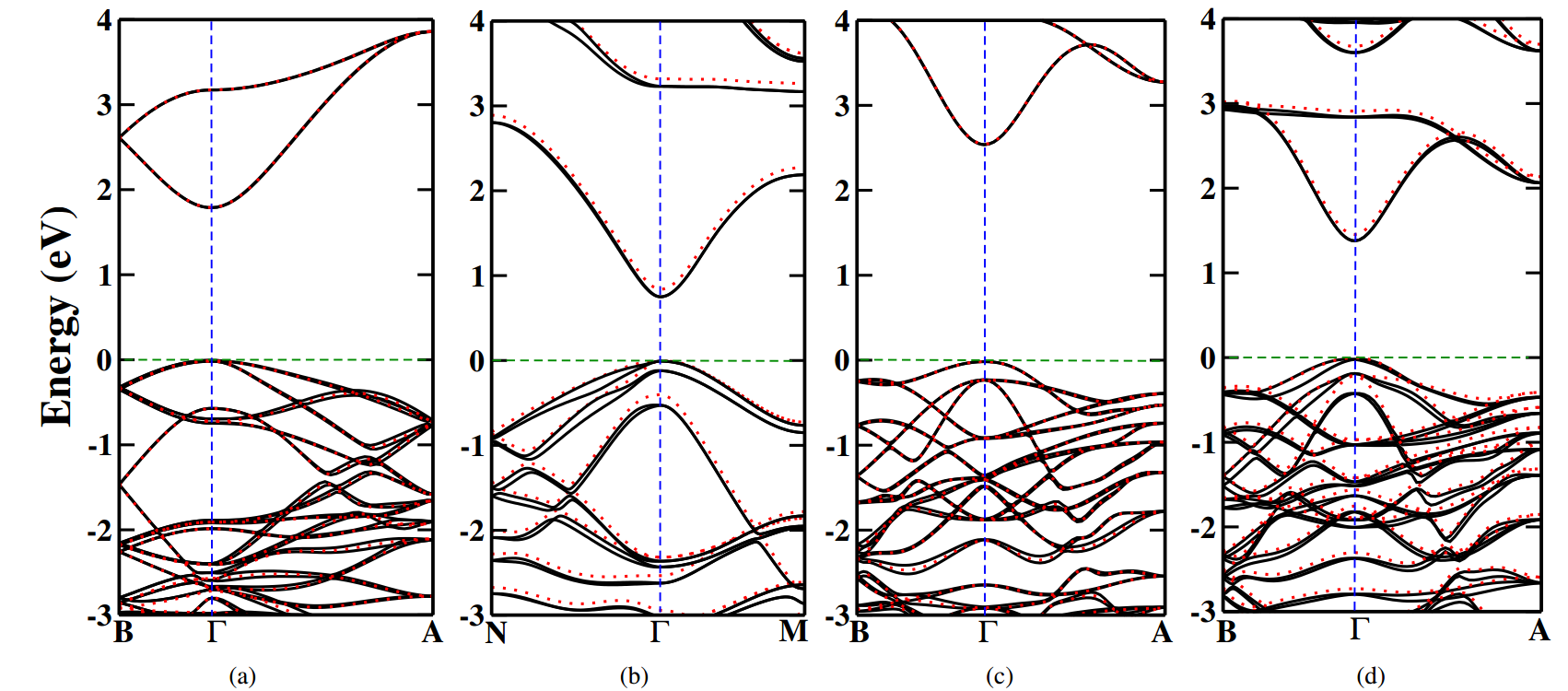
Figure 3: The calculated band structures illustrate the electronic properties of quaternary chalcopyrite: (a) AZS, (b) AZSe, (c) AZGS, and (d) AZGSe. Solid black lines represent results including Spin-Orbit Coupling (SOC), while red dotted lines depict calculations conducted without SOC. These visualizations offer insights into the intricate energy dispersion characteristics of these materials, crucial for understanding their potential applications in transport properties

The reported experimental band gaps for AZTS and AZTSe stand at 2.01 eV and 1.4 eV, respectively, as documented in  Li et al. (2013). Unfortunately, there are no experimental results available for AZGS and AZGSe. Upon introducing spin-orbit coupling (SOC) in our calculations, noticeable shifts in the band gaps were observed. Specifically, the direct-indirect-direct band gap (DDH) of AZTS, AZTSe, AZGS, and AZGSe transitioned from 1.82 eV, 0.94 eV, 2.56 eV, and 1.45 eV to 1.81 eV, 0.86 eV, 2.55 eV, and 1.40 eV, respectively.

Analysis reveals that sulfide quaternary chalcopyrites exhibited minimal alterations with SOC inclusion compared to selenide Ag-based quaternary chalcopyrites. This can be attributed to the negligible impact of SOC in AZTS and AZGS, primarily due to the lighter mass of sulfur compared to selenium. This trend is visually depicted in Figure  3 (a) and (c), showcasing only slight shifts in the top two valence bands of AZTSe and AZGSe, while a distinct shift is evident in the third valence band, as illustrated in Figure  3 (b) and (d). The corresponding data is accessible in Table  3. Consequently, these three valence bands play a significant role in hole transport calculations.

III.3 Effective mass

Table 3: Calculated band gap with SOC;${g}^{SOC}$, without SOC; E${g}^{wSOC}$, and valence band maxima of the three highest valence bands. All these parameters are expressed in electron volts (eV). The effective masses (m^∗) represent the calculated values for the lowest conduction band (1, e) and three highest valence bands (i, h where i=1, 2, 3) along both the perpendicular ($\perp$) and parallel ($\parallel$) axes in AXT, AZTY, and AZGY using DDH. All the effective mass values are in the unit of the free electron mass (m₀).

	AGT	AIT	AZTS	AZTSe	AZGS	AZGSe
E${}_{g}^{SOC}$(eV)	1.06	0.94	1.80	0.86	2.55	1.40
E${}_{g}^{wSOC}$(eV)	1.25	1.17	1.82	0.94	2.56	1.45
E${}_{g}^{exp}$(eV)	1.20	1.04	2.01	1.4	-	-
VBM1,h(eV)	0	0	0	0	0	0
VBM2,h(eV)	-0.002	-0.017	-0.012	-0.0078	-0.006	-0.0051
VBM3,h(eV)	-0.105	-0.077	-0.101	-0.018	-0.166	-0.172
m${}^{*}_{1,e}\perp$	0.091	0.083	0.191	0.116	0.21	0.117
m${}^{*}_{1,e}\parallel$	0.077	0.073	0.186	0.081	0.177	0.107
m${}^{*}_{1,h}\perp$	0.256	0.445	0.679	0.625	0.765	0.525
m${}^{*}_{1,h}\parallel$	0.085	0.083	0.770	0.172	0.215	0.123
m${}^{*}_{2,h}\perp$	0.466	0.387	0.661	0.625	0.781	0.448
m${}^{*}_{2,h}\parallel$	0.086	0.084	0.62	0.155	0.821	0.124
m${}^{*}_{3,h}\perp$	0.138	0.105	0.644	0.355	0.681	0.208
m${}^{*}_{3,h}\parallel$	0.389	0.311	0.611	0.179	0.53	0.563

The effective mass $m^{*}$ of charge carriers in materials, such as electrons or holes in semiconductors, plays a pivotal role in determining their transport properties. Essentially, it represents how a carrier behaves under the influence of external forces, akin to its inertia. A lighter effective mass implies greater carrier mobility, facilitating faster movement in response to electric fields and leading to higher electrical conductivity. Conversely, heavier effective masses hinder carrier mobility, resulting in lower conductivity  Pei et al. (2012).

Additionally, the effective mass is pivotal in influencing various transport phenomena, including the Seebeck coefficient, which defines a material’s thermoelectric properties. Lighter carriers typically exhibit larger variations in mobility with energy, leading to higher Seebeck coefficients. Thus, the effective mass serves as a critical parameter governing the behavior of charge carriers and significantly affecting the overall transport characteristics of materials  Kang and Snyder (2017).

The effective mass tensor for electrons and holes is determined using the equation:

$$m^{*}=\frac{\hbar^{2}}{\frac{\partial^{2}E(\mathbf{k})}{\partial k^{2}}}$$

where $E(\mathbf{k})$ represents the energy dispersion relation, depicting the energy of the particle as a function of its wavevector $\mathbf{k}$. This tensor can be represented in matrix form as:

$$\mathbf{M}=\begin{pmatrix}m_{11}&m_{12}&m_{13}\\ m_{12}&m_{22}&m_{23}\\ m_{13}&m_{23}&m_{33}\end{pmatrix}$$

In isotropic materials, such as those with a diagonal effective mass tensor, all off-diagonal elements are zero, retaining components $m_{11}$, $m_{12}$, and $m_{13}$  Remsing and Bates (2020). Here, $m_{11}$ and $m_{12}$ represent the transverse effective mass along the $a$ and $b$ directions, referred to as $m^{*}_{i,j}\parallel$, while $m_{13}$ represents the longitudinal effective mass along the $c$ direction, denoted as $m^{*}_{i,j}\perp$.

The effective mass of electrons in the conduction band and holes in the three topmost valence bands is computed along the longitudinal and transverse directions for all six materials, as indicated in Table  3. This computation involves fitting the band structure data (energy versus $\mathbf{k}$) near the $\Gamma$ point for both parallel and perpendicular directions. The electrons and holes are lighter in ternary compounds than quaternary compounds. The heaviest electron has an effective mass of 0.191 $m_{0}$ in the perpendicular direction for AZTS quaternary chalcopyrite. In contrast, the heaviest hole for ternary compounds has an effective mass of 0.466 $m_{0}$, which is lighter than the heaviest hole in quaternary chalcopyrite with an effective mass of 0.821 $m_{0}$. Next, we will examine the effect of these effective masses on the transport properties of these materials.

III.4 Electron Transport Properties

To analyze electronic transport properties, we employ the semi-classical Boltzmann transport equation (BTE) within the relaxation time approximation (RTA) Zhou et al. (2010), using the BoltzTraP2 (BTP2) code Madsen et al. (2018). Our calculations spanned the temperature range from 600 to 800 K, with 100 K increments, and encompassed hole carrier concentrations up to $10^{23}$ cm^-3. Within the BTE framework, we determine the Seebeck coefficient ($S$), electrical conductivity ($\sigma$), and electronic contribution to thermal conductivity ($\kappa_{e}$) through the Onsager coefficients, as defined below:

$$S =\frac{1}{qT}\cdot\frac{L_{x,y}^{1}}{L_{x,y}^{0}},$$ (2)

$$\sigma =L_{x,y}^{0},$$ (3)

$$\kappa_{e} =\frac{1}{q^{2}T}\left(L_{x,y}^{2}-\frac{L_{x,y}^{1}}{L_{x,y}^{0}}\right),$$ (4)

where $q$ represents the elementary charge, and $L_{x,y}^{i}$ denotes the kernel of the generalized transport coefficient at temperature T can be expressed as: Nag (2012)

$$L_{x,y}^{i}=q^{2}\sum_{x,y}\tau_{x,y}v^{2}_{x,y}(\varepsilon_{x,y}-\mu)^{i}\left(-\frac{\partial f_{x,y}}{\partial\varepsilon_{x,y}}\right),$$ (5)

with $i=0,1,2$. Here, $\tau_{x,y}$, $v_{x,y}$, $\varepsilon_{x,y}$, and $f_{x,y}$ respectively represent the electronic relaxation time, group velocity, energy, and Fermi-Dirac distribution function of the $x$th band at wave vector $y$. Based on the equations 3,  4 and  5 calculating the $\sigma$ and $\kappa_{e}$ parameters require the relaxation time $\tau$ as an input. This parameter can be calculated using the constant-relaxation-time approximation (CRTA), as outlined in References Pal et al. (2019); Hasan et al. (2022); Hao et al. (2019), the constant $\tau=\tau_{0}$ will be extracted from the integrals that determine the Onsager coefficients.

In this context, the BTP2 code provides reduced coefficients $\sigma_{0}=\sigma/\tau_{0}$ and $\kappa_{e,0}=\kappa_{e}/\tau_{0}$, determined by factors such as band structure, temperature, and doping, yet independent of $\tau_{0}$. Subsequently, $ZT$ is derived from these reduced transport coefficients, assuming specific values for the relaxation time $\tau_{0}$. The CRTA approach assumes a constant relaxation time $\tau$ across all energy levels. Consequently, while the power factor relies on $\tau$, the figure of merit $ZT$ remains unaffected by variations in $\tau$. Recognizing this limitation of CRTA, we opt to employ an alternative method to determine $\tau$.

To assess the electronic transport characteristics, the deformation potential theory Bardeen and Shockley (1950); Xi et al. (2012) is utilized to analyze the relaxation time. Within the framework of the single parabolic band (SPB) model, the relaxation time for the three-dimensional system is expressed as Ning et al. (2020); Shuai et al. (2012):

$$\tau=\frac{1}{3}\times 2\sqrt{{2}{\pi}}\frac{C\hbar^{4}}{(k_{B}Tm_{\text{dos}^{*}})^{\frac{3}{2}}}\left(\frac{1}{D}\right)^{2}$$ (6)

Here, $\hbar$ represents the reduced Planck constant, $C$ denotes the elastic constant, $k_{B}$ is the Boltzmann constant, $m_{\text{dos}^{*}}$ signifies the effective mass of the density of states (as we focus on a p-type system, we consider only the effective mass of holes), and $D$ refers to the deformation potential energy.

Table 4: The calculated single-crystal elastic constants C_ij (expressed in GPa), Deformation Potentials for both electrons D(e) and holes D(h) (in electron volts, eV), longitudinal (v_L; measured in meters per second, m/s), transverse (v_T; in m/s), average sound velocity ($\bar{v}$; in m/s), and Debye temperature ($\Theta_{D}$:measured in K) for materials AXT, AZTY, and AZGY (where (X=G,I); (Y=S/Se)) utilizing the Dielectric Dependent Hybrid approach.

	AGT	AIT	AZTS	AZTSe	AZGS	AZGSe
C11	53.90	49.55	72.11	55.99	83.27	75.97
C12	30.99	31.47	58.26	43.28	51.75	48.04
C13	33.82	30.94	37.45	41.06	60.99	47.14
C33	52.72	48.24	68.01	71.26	83.22	75.97
C44	41.38	35.23	25.81	41.14	51.71	47.267
C66	36.60	34.24	59.24	46.70	51.50	46.28
D(e)	5.31	9.08	11.23	9.22	14.19	8.09
D(h)	4.49	8.61	8.82	7.79	10.35	6.88
vL	3527.86	3373.97	3845.77	4222.68	5217.12	4117.47
vT	2020.93	1899.99	3895.31	2605.64	3253.21	2248.92
$\bar{v}$	2245.14	2113.82	3878.51	2874.30	3584.63	2508.03
$\Theta_{D}$	211.3	192.2	403.20	284.6	380.4	253.3

To determine the electronic relaxation time ($\tau$), we computed the single-crystal elastic constants $C_{ij}$ for both ternary and quaternary chalcopyrites. All materials under investigation in this study exhibit a tetragonal structure Vajeeston and Fjellvåg (2017), characterized by six independent elastic constants: $C_{11}$, $C_{12}$, $C_{13}$, $C_{33}$, $C_{44}$, and $C_{66}$, which adhere to mechanical stability criteria given by:

$$C_{11}>C_{12}$$ (7)

$$2C^{2}_{13}<C_{33}(C_{11}+C_{12})$$ (8)

$$C_{44}>0$$ (9)

$$C_{66}>0$$ (10)

The calculated elastic constants for AXT (where X = Ga, In)and AZPQ (where P=Sn, Ge and Q= S, Se) are presented in Table 4, satisfying Equations 7, 8, 9, and 10. The deformation potential ($D$) for the conduction band (electrons) and the valence band (holes) is determined from the strained and unstrained band structures. Subsequently, $\tau$ is evaluated using Equation 6, and the resulting $\tau$ values are plotted against temperature ranging from $300K$ to $800K$ in Figure 6 (a). The relaxation time is expressed in units of $10^{-14}$ s. Notably, the relaxation time increase with increasing temperature. Among the materials studied, the quaternary chalcopyrite AZGSe exhibits the lowest relaxation time, while AIT demonstrates the highest relaxation time. At $800K$, the relaxation time for ternary chalcopyrites AGT and AIT is observed to be $0.98\times 10^{-14}$ s and $0.44\times 10^{-14}$ s, respectively. Contrastingly, quaternary chalcopyrites AZTS, AZTSe, AZGS, and AZGSe exhibit relaxation times ranging from $1.23$ , $1.48$, $0.95$, $2.03$ multiples of $10^{-14}$ s. This disparity suggests that quaternary chalcopyrites undergo more frequent scattering interactions with lattice defects, phonons, and other charge carriers, leading to accelerated relaxation compared to ternary counterparts.

III.4.1 AXT

Given the band structure of AXT (where X represents Ga or In) as shown in  2 (a) and (b), our study facilitates the computation of crucial transport parameters, including the Seebeck coefficient, electrical conductivity, and thermal conductivity, utilizing the Boltzmann Transport Equation (BTE) in conjunction with the Relaxation Time Approximation (RTA). Our methodology meticulously incorporates the lowest conduction band and three valence bands proximal to the $\Gamma$ (Gamma) point, while also accounting for the spin degeneracy of each band. Within the context of these p-type wide bandgap semiconductors, our analyses reveal a diminished influence of the bipolar effect, with hole carriers assuming prominence in dictating the transport phenomena.

Figure 4: The calculated (a) Seebeck coefficient, (b) electrical conductivity, (c) electron thermal conductivity, and (d) power factor versus carrier concentration are depicted for AGT and AIT at temperatures of 600 K, 700 K, and 800 K.

Equations (2), (3), and (4) illustrate the key parameters. In p-type wide band gap semiconductors, the influence of the bipolar effect is minimal, with hole carriers overwhelmingly dictating transport properties. As temperature rises, relaxation time diminishes due to heightened phonon scattering. Doping emerges as a viable means to enhance electrical conductivity. Our findings align closely with those reported in Yang et al.  Yang et al. (2017) for AGT and AIT materials. Utilizing the relaxation time ($\tau$) derived from Deformation Potential Theory, as discussed above, we computed the electrical conductivity ($\sigma$) and electrical thermal conductivity ($\kappa_{e}$) in the forms of $\sigma/\tau$ and $\kappa/\tau$, respectively, employing Boltzmann Transport Equation (BTE) theory. At higher temperatures, there’s a possibility of minority carrier generation, which can influence the conduction mechanism. This phenomenon, often termed as bipolar thermal conduction, becomes dominant particularly at high temperatures and low carrier concentrations.

Figure  4 illustrates the dependence of carrier concentration (n) on S, $\sigma$, S${}^{2}\sigma$, and electronic thermal conductivity ($\kappa_{e}$). It’s evident that S decreases as n increases, whereas $\sigma$ exhibits an opposite trend, ultimately contributing to the enhancement of power factor (S${}^{2}\sigma$). The latter peaks at an optimal carrier concentration before declining. At high temperatures and low carrier concentrations (n), the bipolar effect becomes evident, affecting the electronic thermal conductivity ($\kappa_{e}$). The peaks in TE coefficients occur at varying carrier concentrations for AGT and AIT conduction, owing to differences in band topology and resulting scattering rates. The power factor (P.F.) for AGT aligns comparably with TE materials from ternary chalcopyrites. The optimal S${}^{2}\sigma$ value is 27.7 $\mu$W/cmK² at a hole doping of 5.35 × 10²⁰ cm^-3 at 800 K, as depicted in Figure 4 (d), comparable to the P.F. of 25 $\mu$W/cmK² at an optimal carrier concentration of 8.7 × 10²⁰ cm^-3 for CuGaTe₂, belonging to the same category  Wang et al. (2017). The significant enhancement in electrical conductivity primarily contributes to these high P.F. values. However, AIT, with an optimal P.F. of 13.53 $\mu$W/cmK² at a hole concentration of 2.5 × 10²⁰ cm^-3 even at even at 800 K, falls outside the standard range of TE materials. Nevertheless, its values can potentially be improved through further doping or defect studies.

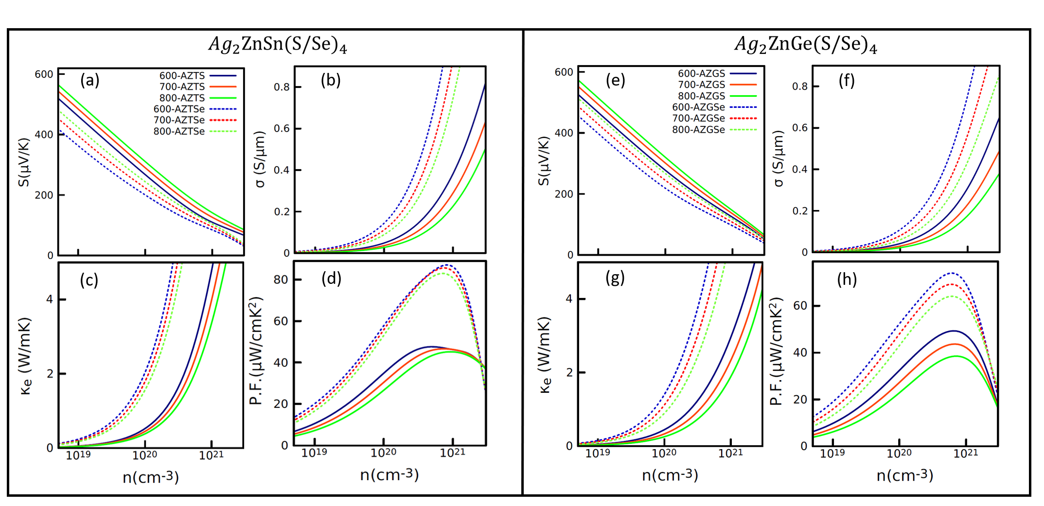
Figure 5: The graph plots the (a)/(e) Seebeck coefficient, (b)/(f) electrical conductivity, (c)/(g) electron thermal conductivity, and (d)/(h) power factor against carrier concentration for Ag₂ZnSn(S/Se)₄ (on the left) and Ag₂ZnGe(S/Se)₄ (on the right) across temperatures of 600 K, 700 K, and 800 K.

III.4.2 AZPQ

Comprehending the transport properties of quaternary chalcopyrites presents a more intricate task compared to their ternary counterparts. This complexity stems from the introduction of an additional element and the resulting intricate interactions within the material  Li et al. (2013). Through the analysis of the scattering time ($\tau$) and lattice thermal conductivity ($\kappa_{l}$), we can extract valuable insights into the mechanisms governing heat and charge transport within these materials  Hasan et al. (2022).

In AZPQ-type compositions, the incorporation of an extra element relative to ternary chalcopyrites grants finer control over several crucial properties. These include the material’s band gap, carrier concentration, and the scattering mechanisms influencing transport. This heightened level of control proves beneficial in applications requiring specific transport characteristics, such as high electrical conductivity for thermoelectric devices or low thermal conductivity for effective heat dissipation.

The Seebeck coefficient ($S$), a crucial parameter in thermoelectric materials, demonstrates a notable enhancement for AZPQ materials as shown in Fig   5(a) and (e) compared to their AXT counterparts within the same range of hole doping concentration (Figure 4). This observation suggests that AZPQ materials possess a greater ability to convert thermal gradients into electrical voltage due to their superior ability to hold onto charge carriers (higher effective mass or reduced carrier scattering). This is further supported by the significantly higher electrical conductivity ($\sigma$) observed for AZPQ materials compared to AXT counterparts (Figure 5 (b) and (f)). The superior electrical transport properties of AZPQ materials translate to a remarkable improvement in the power factor (PF), a metric that combines $S$ and $\sigma$. As shown in Figure 5 (h), the optimal PF for AZTSe reaches a value of 87.5 $\mu$W/cmK² at a hole doping concentration of $8.2\times 10^{20}$ cm^-3. This value is significantly higher compared to the 47.7 $\mu$W/cmK² achieved by AZTS material at a lower doping concentration ($5.4\times 10^{20}$ cm^-3) in Figure  5 (d).

On the contrary, AZGSe and AZGS, both Ge-based materials, demonstrate a P.F. (S²$\sigma$) of 74.7 $\mu$W/cmK² and 49.4 $\mu$W/cmK², respectively, at a hole doping level of 6.2 $\times$ 10${}^{2}0$ cm^-3 in Figure  5 (h). Comparing Sn and Ge based materials, it’s evident that Se-based compounds exhibit higher P.F. compared to S-based ones. If the total thermal conductivity ($\kappa_{e}$ +$\kappa_{l}$) follows a similar trend, favoring Se-based materials, they could outperform S-based materials in terms of TE performance. This is because a higher $\kappa$ facilitates heat flow through the material, reducing the temperature gradient and consequently the voltage generated by the Seebeck effect. In essence, while Se-based materials might excel in voltage generation from a thermal gradient, their potential suffers if their overall thermal conductivity is too high. Optimizing a TE material requires careful consideration of these competing factors to achieve a maximized ZT and efficient thermoelectric conversion.

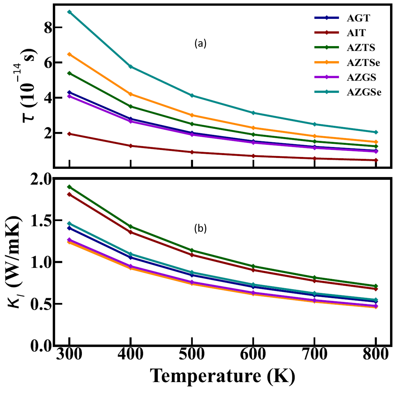
Figure 6: The computed relaxation time and lattice thermal conductivity obtained through Equations  6 and  11, covering the temperature range from 300K to 800K.

III.5 Lattice thermal transport

Optimizing the thermoelectric figure of merit (ZT) requires careful consideration of the thermal conductivity ($\kappa$), which encompasses both electronic ($\kappa_{e}$) and lattice ($\kappa_{l}$) contributions. While the Boltzmann transport equation (BTE) framework, detailed in equation (4), can be used to calculate $\kappa_{e}$, obtaining $\kappa_{l}$ via the full linearized phonon BTE is computationally expensive due to the complexity of phonon calculations Ziman (2001); Li et al. (2014). To address this challenge, we can leverage a simpler approach known as Slack’s equation to estimate $\kappa_{l}$ Jia et al. (2017); Morelli et al. (2008). This method offers a practical alternative for materials simulations, particularly when dealing with complex phonon interactions.

$$\kappa_{l}=A\frac{\delta\overline{M}\Theta^{3}}{\gamma^{2}n^{2/3}T}$$ (11)

where $\delta^{3}$, $\overline{M}$, $\Theta$, $\gamma$, $n$, and $T$ represent the volume per unit atom, the average atomic mass, the acoustic Debye temperature, the acoustic Grüneisen parameter, the number of atoms in the primitive unit cell, and temperature, respectively. Here, $A$ is a constant given by:

$$A=\frac{2.43\times 10^{-8}}{1-\frac{0.514}{\gamma}+\frac{0.228}{\gamma^{2}}}$$ (12)

Equation 11 is extensively utilized for evaluating lattice thermal conductivity Morelli et al. (2008); Nielsen et al. (2013); Shindé and Goela (2006); Bruls et al. (2005); Skoug et al. (2010). The Debye temperatures and Grüneisen parameters of acoustic branches can be accurately determined using phonon dispersions obtained from lattice dynamic calculations or experimental measurements. For computing $\Theta$ and $\gamma$, we adopt the approach proposed by Xiao et al. Xiao et al. (2016), which utilizes an efficient formula based on elastic properties, Poisson ratio $\nu$, or sound velocity, to estimate the Grüneisen parameter given by Sanditov et al. (2009); Jia et al. (2017):

Table 5: The Voigt, Reuss, and Hill bulk moduli, shear moduli, Young’s moduli, Poisson’s ratios, and the ratio of bulk to shear modulus were calculated for AXT (where X = Ga, In), AZTY, and AZGY with Y being S or Se.

	B(GPa)			G(GPa)			E(GPa)			$\eta_{p}$			B/G
	VOIGT	REUSS	HILL	VOIGT	REUSS	HILL	VOIGT	REUSS	HILL	VOIGT	REUSS	HILL	VOIGT	REUSS	HILL
AGT	39.76	39.75	39.76	28.00	18.38	23.19	68.03	47.78	58.25	0.21	0.30	0.26	1.42	2.16	1.71
AIT	37.12	37.10	37.11	24.56	16.22	20.39	60.37	42.47	51.70	0.23	0.30	0.27	1.51	2.28	1.82
AZTS	55.01	51.50	52.35	23.44	19.05	20.43	56.7	49.99	52.87	0.27	0.33	0.31	2.34	2.70	2.56
AZTSe	48.23	47.74	47.98	56.97	17.26	13.11	122.63	46.20	88.52	0.08	0.33	0.19	0.85	2.76	1.29
AZGS	59.41	59.31	59.36	18.10	77.76	47.93	49.29	162.35	113.30	0.36	0.04	0.18	3.28	0.76	1.23
AZGSe	55.69	55.09	55.38	33.93	20.94	27.43	84.61	55.76	70.64	0.25	0.33	0.28	1.64	2.63	4.31

$$\gamma=\frac{3}{2}\Big{(}\frac{1+\nu}{2-3\nu}\Big{)}$$ (13)

The method based on sound velocity for determining the Grüneisen parameter is computationally more feasible than quasiharmonic phonon calculations Xiao et al. (2016). The Poisson ratio $\nu$ is expressed as a function of the shear wave (v_S) and longitudinal wave (v_L) sound velocities, respectively:

$$\nu=\frac{1-2(\frac{v_{S}}{v_{L}})^{2}}{2-2(\frac{v_{S}}{v_{L}})^{2}}$$ (14)

The sound velocities v_L and v_S, and the corresponding average velocity ($\overline{v}$), are given by Kinsler et al. (2000):

$$v_{L}=\sqrt{\frac{B+4/3G}{\rho}},\quad v_{S}=\sqrt{\frac{G}{\rho}},\quad\overline{v}=\Big{[}\frac{1}{3}\Big{(}\frac{1}{v_{L}^{3}}+\frac{2}{v_{S}^{3}}\Big{)}\Big{]}^{-1/3}$$ (15)

where $B$, $G$, and $\rho$ represent the bulk modulus, shear modulus, and density of the compound, respectively. The Debye temperature of acoustic phonons $\Theta$ is given by Anderson (1963):

$$\Theta=\frac{h}{k_{B}}\Big{[}\frac{3m}{4\pi}\Big{]}^{1/3}\overline{v}n^{-1/3}$$ (16)

Here, $h$, $k_{B}$, and $m$ are the Planck constant, Boltzmann constant, and the number of atoms per volume, respectively, and $n$ represents the number of atoms in the primitive cell. The term $n^{-1/3}$ is used to roughly separate the acoustic branches from the total vibration spectrum Anderson (1963).

To determine the lattice thermal conductivity ($\kappa_{l}$), which predominantly contributes (98$\%$), Equation 4 was utilized after computing essential mechanical properties of the materials. These properties, including Bulk Modulus ($B$), Shear Modulus ($G$), and Elastic Modulus ($E$), were directly derived from the elastic constants tensors Vajeeston and Fjellvåg (2017). Subsequent calculations involved longitudinal ($v_{L}$) and transverse ($v_{T}$) velocities, along with the average velocity $\bar{v}$, as depicted in Table 4 to determine the Poisson’s ratio. The values of $B$, $G$, $E$, Poisson ratio ($\eta_{p}$), and Bulk-to-Shear Modulus ratio were determined using the Voigt-Reuss-Hill approximations Reuß (1929); Hill (1952) as shown in the Table  5. The $B/G$ ratio was assessed to discern the material’s brittleness or ductility, with values below 2 indicating ductile behavior. Once the average velocity was established, the Debye Temperature ($\theta_{D}$) was calculated using Equation 16, listed in Table 4 for all materials. Subsequently, $\kappa_{l}$ was evaluated according to Equation 4. The lattice thermal conductivity, measured in units of W/mK, was then plotted against temperature in Figure 6 (b). Notably, a decrease in lattice thermal conductivity with increasing temperature was observed. To validate this method’s accuracy, our results for AGT and AIT were compared with lattice thermal conductivity values provided in reference  Yang et al. (2017). Additionally, it was observed that among all materials, quaternary chalcopyrite AZTS exhibited the highest while AZTSe displayed the lowest lattice thermal conductivity. This disparity in lattice thermal conductivities between quaternary chalcopyrites AZTSe and AZGS underscores the intricate physics governing thermal transport phenomena in these materials. The optimized values of $\kappa_{l}$ were determined to be 0.52, 0.67, 0.71, 0.45, 0.46, and 0.54 W/mK, for AGT, AIT, AZTS, AZTSe, AZGS, AZGSe respectively, at 800K.

Furthermore, considering the implications on the Figure of Merit $ZT$, where $\sigma$ and $\kappa_{e}$ are functions of $\tau$ according to Boltzmann Theory, the total thermal conductivity is the sum of $\kappa_{e}$ and $\kappa_{l}$.

III.6 Figure of merit

An accurate estimation of ZT requires an accurate calculation of the electron relaxation time ($\tau$) and lattice Thermal conductivity ($\kappa_{l}$).

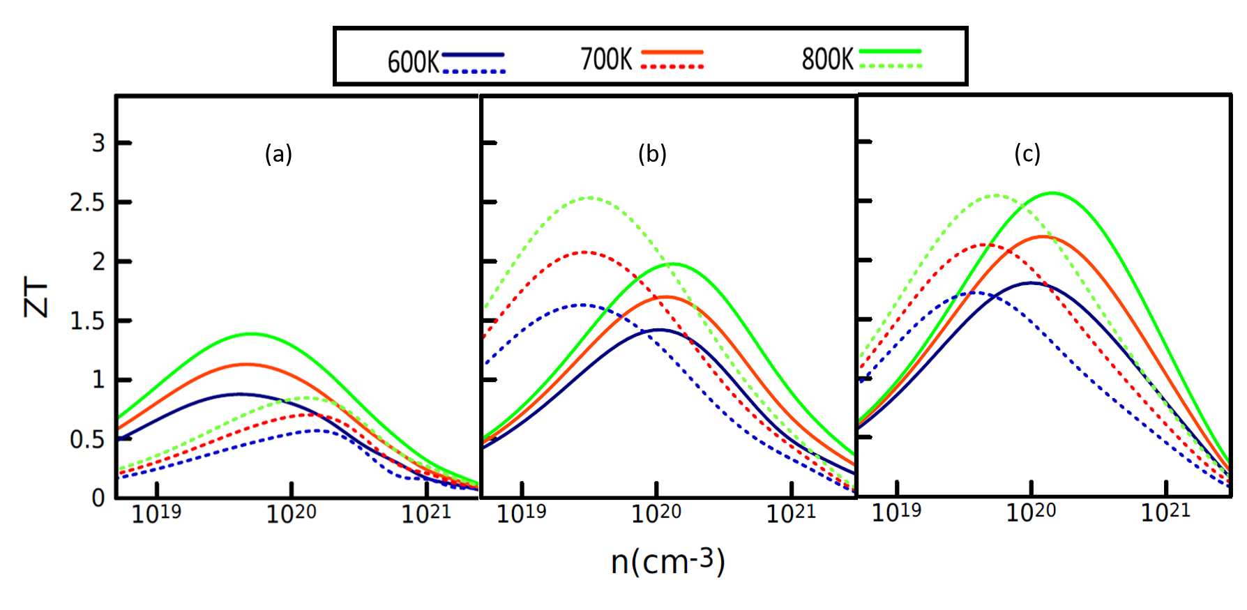
Figure 7: The graphical representation illustrates the computed thermoelectric figure of merit ZT versus carrier concentration across temperatures of 600 K, 700 K, and 800 K for various compounds:(a) Solid lines depict the ZT values for AGT, contrasting with the representation of ZT for AIT shown by dotted lines. (b) Solid lines correspond to AZTS, while dotted lines represent AZTSe. (c) The ZT values for AZGS and AZGSe are respectively illustrated by solid and dotted lines.

The inherent structural complexity of ternary and quaternary chalcopyrites, characterized by low symmetry and large unit cells, poses a formidable challenge for many-body calculations of $\tau$. We employ the deformation potential (DP) method, which accounts for the interactions between charge carriers and acoustic phonons, as initially proposed by Bardeen and Shockley as given in Section  III.4. Note that, although the DP approach overlooks Coulombic scattering from polar-optical vibrations, the vibration of ions with opposite charges. it has been an effective approximation for calculations of TE materials. This effectiveness is grounded in fundamental physical principles. According to the Fröhlich model  Huang and Zhu (1988), the Coulombic interaction, known as electron-optical-polar scattering, can be effectively screened by using the optical ($\epsilon_{\infty}$) and static ($\epsilon_{s}$) dielectric constants. As discussed in the previous work  Deng et al. (2021), large dielectric constants are prerequisites for being workable TE materials, the feature that also turns DP into a reasonable approach in this context. By using $\tau$ and $\kappa_{l}$ we have calculated figure of merit ZT for all our compounds as shown in Figure  7. Note that the relaxation time decreases with increasing temperature, roughly following a $T^{-3/2}$ relationship as denoted in equation  6 and previous work.   So, the variation of ZT with temperature almost resembles a dome-shaped curve. For our system ZT reaches maximum at 800 K. we have plotted the ZT values for our system in the range of 600-800 K. For p-type thermoelectric materials, the electronic concentration and electron thermal excitation are obvious at room at low hole concentration and high temperature. We can see in Figure  7(a-c), at lower hole concentration the difference between ZT values for different temperature is less because of the thermal excitation. As we can see, the figure of merit ZT heavily depends on carrier concentration and temperature. There are few calculations of figure of merit for AGT and AIT has been done in literature.  Plata et al. (2023); Parker and Singh (2012); Zhong et al. (2021) Based on our calculations in figure  7 (a), AGT demonstrates nearly isotropic ZT values of 1.14 and 1.40 at temperatures of 700 K and 800 K, respectively, with a hole carrier concentration of $4.88\times 10^{19}$ cm^-3. These ZT values signify the material’s ability to efficiently convert heat differentials into electrical energy, making it a promising candidate for high-temperature thermoelectric (TE) applications. Conversely, AIT’s maximal ZT of 0.86 at a hole doping level of $1.29\times 10^{20}$ cm^-3 suggests limitations in its electron transport properties, resulting in less effective thermal energy conversion compared to AGT. This failure to achieve a ZT value above 1 underscores AIT’s unsuitability for TE devices. Furthermore, at 600 K, AGT’s ZT value of 0.90 at a hole doping of $10^{19}$ cm^-3 indicates suboptimal electron mobility, which diminishes its potential as a TE material in lower-temperature regimes.

In the realm of quaternary chalcopyrites, there have been no experimental validations for our top suggested TE quaternary chalcogenides, particularly those based on Ag. Se-based quaternary chalcopyrites are expected to have a higher figure of merit compared to S-based ones, according to the power factor (P.F.) comparison between these materials as shown in Figure  5 (d) and (h). For AZTS, the maximum ZT (Figure  7 (b)) of 1.98 at 800 K is achieved with a hole doping of $1.34\times 10^{20}$ cm^-3, whereas AZTSe exhibits a hole doping of $3.25\times 10^{19}$ cm^-3, resulting in a ZT of 2.53 at 800 K. Interestingly, AZTSe and AZTS achieve optimal ZT values at different hole doping levels. Hole-doped AZGS achieves a nearly isotropic ZT of 2.57 at 800 K. It’s worth noting that AZGS, like the majority of other quaternary chalcogenides with CST networks, features a quasi-linear conduction band, leading to nearly negligible n-type thermoelectric behavior.AZGSe also falls within the category of p-type thermoelectric materials, achieving ZT values of 1.72 at 600 K, 2.13 at 700 K, and 2.55 at 800 K, with hole concentrations of $4.9\times 10^{19}$, $5.8\times 10^{19}$, and $7\times 10^{19}$ cm^-3, respectively.An intriguing observation is that while the power factor of AZGSe is higher than that of AZGS, as shown in Figure  5 (h), the figure of merit of AZGS is greater than AZGSe, incorporating the effect of lattice thermal conductivity ($\kappa_{l}$) as seen in Figure  6. Specifically, AZGS possesses lower lattice thermal conductivity compared to AZGSe. This difference in lattice thermal conductivity contributes to AZGS having a higher figure of merit than AZGSe, contrary to initial expectations, as shown in Figure  7 (c). Among the six materials under study, all except AIT demonstrate ZT values exceeding 1 at high hole doping concentrations ($10^{19}$ - $10^{20}$ cm^-3), positioning them as robust candidates for thermoelectric (TE) applications. This phenomenon underscores their potential to efficiently convert waste heat into electrical power. However, it’s crucial to acknowledge the inherent complexities of real-world materials compared to idealized models based on density functional theory (DFT) calculations. Laboratory-synthesized samples may encounter various scattering mechanisms that can significantly influence their thermoelectric properties, highlighting the need for experimental validation and further investigation.

Moreover, beyond merely boasting a high figure of merit, thermoelectric materials must also exhibit exceptional dopability to tailor their electronic properties effectively. Notably, diamond-like chalcogenides have garnered attention for their outstanding p-type dopability, enabling precise control over band structures and electron behavior. This characteristic holds promise for enhancing thermoelectric efficiencies and advancing sustainable energy conversion technologies, offering a pathway towards practical implementation in diverse applications.

IV Conclusions

We’ve employed a comprehensive approach, integrating multiband Boltzmann transport equations with first-principles calculations utilizing the Non-empirical Range-separated Dielectric-dependent Hybrid (DDH) Approach. This methodology enables us to accurately capture the electronic band structures, crucial for theoretical exploration of thermoelectric (TE) properties in ternary and quaternary Ag-based chalcopyrites. Among these materials, AZGS emerges with the highest band gap of 2.52 eV, coupled with substantial spin-orbit coupling effects, primarily attributed to S-atoms. These features contribute significantly to favorable electronic transport parameters. In our analysis of charge carrier scattering interactions with acoustic phonons, we’ve incorporated the Deformation Potential Theory to calculate electron relaxation time. The resultant values align well with experimental data (when available), validating our theoretical framework. The figure of merit ZT hinges greatly on Seebeck coefficient and electron conductivity, while being influenced by thermal conductivity, which encompasses contributions from both electron and lattice thermal conductivity. Instead of resorting to computationally expensive harmonic phonon calculations, we’ve utilized computationally feasible elastic properties to estimate lattice thermal conductivity. Employing these methods, we’ve identified AZGS as the premier thermoelectric material, exhibiting a ZT value of 2.57 at 800 K, surpassing all other studied materials. Additionally, AZGSe and AZTSe demonstrate promising TE behavior with ZT values of 2.55 and 2.53 at 800 K, respectively. AZTS also emerges as a strong TE candidate, boasting a ZT of 1.98 at 800 K. Overall, the quaternary chalcopyrites exhibit favorable TE performance across the 600-800 temperature range. Although AGT demonstrates promising TE characteristics at high temperatures, it falls short at lower temperatures.

Our methodology, coupled with the highly accurate DDH exchange-correlation approximation, underscores the suitability of our materials for further applications in thermoelectric devices, offering promising avenues for practical implementation and advancement in sustainable energy conversion technologies.

References

- DiSalvo (1999) F. J. DiSalvo, Science 285, 703 (1999).
- Bell (2008) L. E. Bell, Science 321, 1457 (2008).
- Leonov and Vullers (2009) V. Leonov and R. J. Vullers, Journal of Renewable and Sustainable Energy 1 (2009).
- Boyer and Cisse (1992) A. Boyer and E. Cisse, Materials Science and Engineering: B 13, 103 (1992).
- Lv et al. (2022) L.-Y. Lv, C.-F. Cao, Y.-X. Qu, G.-D. Zhang, L. Zhao, K. Cao, P. Song, and L.-C. Tang, Materials Science and Engineering: R: Reports 150, 100690 (2022).
- Mahan and Sofo (1996) G. Mahan and J. Sofo, Proceedings of the National Academy of Sciences 93, 7436 (1996).
- Heremans et al. (2008) J. P. Heremans, V. Jovovic, E. S. Toberer, A. Saramat, K. Kurosaki, A. Charoenphakdee, S. Yamanaka, and G. J. Snyder, Science 321, 554 (2008).
- Hong et al. (2018) M. Hong, Z.-G. Chen, and J. Zou, Chinese Physics B 27, 048403 (2018).
- Gelbstein et al. (2005) Y. Gelbstein, Z. Dashevsky, and M. Dariel, Physica B: Condensed Matter 363, 196 (2005).
- Downie et al. (2014) R. Downie, D. MacLaren, and J.-W. Bos, Journal of Materials Chemistry A 2, 6107 (2014).
- Cao et al. (2020) Y. Cao, X. Su, F. Meng, T. P. Bailey, J. Zhao, H. Xie, J. He, C. Uher, and X. Tang, Advanced Functional Materials 30, 2005861 (2020).
- Parker and Singh (2012) D. Parker and D. J. Singh, Physical Review B 85, 125209 (2012).
- Charoenphakdee et al. (2009) A. Charoenphakdee, K. Kurosaki, H. Muta, M. Uno, and S. Yamanaka, Materials transactions 50, 1603 (2009).
- Sharma et al. (2014) S. Sharma, A. Verma, and V. Jindal, Materials Research Bulletin 53, 218 (2014).
- Peng et al. (2014) H. Peng, C. Wang, and J. Li, Physica B: Condensed Matter 441, 68 (2014).
- Yang et al. (2017) J. Yang, Q. Fan, and X. Cheng, Royal Society Open Science 4, 170750 (2017).
- Li et al. (2013) K. Li, B. Chai, T. Peng, J. Mao, and L. Zan, Rsc Advances 3, 253 (2013).
- Kaya et al. (2015) W. Kaya et al. (2015).
- Chagarov et al. (2016) E. Chagarov, K. Sardashti, A. C. Kummel, Y. S. Lee, R. Haight, and T. S. Gershon, The Journal of chemical physics 144 (2016).
- Xianfeng et al. (2013) Z. Xianfeng, T. Kobayashi, Y. Kurokawa, S. Miyajima, and A. Yamada, Japanese Journal of Applied Physics 52, 055801 (2013).
- Yeh and Cheng (2014) L.-Y. Yeh and K.-W. Cheng, Thin Solid Films 558, 289 (2014).
- Chen et al. (2009) S. Chen, X. Gong, A. Walsh, and S.-H. Wei, Applied Physics Letters 94 (2009).
- Nainaa et al. (2019) F. Z. Nainaa, N. Bekkioui, A. Abbassi, and H. Ez-Zahraouy, Computational Condensed Matter 19, e00364 (2019).
- Snyder and Toberer (2008) G. J. Snyder and E. S. Toberer, Nature materials 7, 105 (2008).
- Zhou et al. (2010) J. Zhou, X. Li, G. Chen, and R. Yang, Physical Review B 82, 115308 (2010).
- Chung and Buessem (1967) D. Chung and W. Buessem, Journal of Applied Physics 38, 2535 (1967).
- Chen et al. (2018) W. Chen, G. Miceli, G.-M. Rignanese, and A. Pasquarello, Phys. Rev. Mater. 2, 073803 (2018).
- Cui et al. (2018) Z.-H. Cui, Y.-C. Wang, M.-Y. Zhang, X. Xu, and H. Jiang, The Journal of Physical Chemistry Letters 9, 2338 (2018).
- Ghosh et al. (2024) A. Ghosh, S. Jana, D. Rani, M. Hossain, M. K. Niranjan, and P. Samal, Physical Review B 109, 045133 (2024).
- Jana et al. (2023) S. Jana, A. Ghosh, L. A. Constantin, and P. Samal, Physical Review B 108, 045101 (2023).
- Kresse and Furthmüller (1996a) G. Kresse and J. Furthmüller, Physical review B 54, 11169 (1996a).
- Kresse and Furthmüller (1996b) G. Kresse and J. Furthmüller, Computational materials science 6, 15 (1996b).
- Perdew et al. (1996) J. P. Perdew, K. Burke, and M. Ernzerhof, Physical review letters 77, 3865 (1996).
- Kresse and Joubert (1999) G. Kresse and D. Joubert, Physical review b 59, 1758 (1999).
- Woo et al. (1997) T. K. Woo, P. M. Margl, P. E. Blöchl, and T. Ziegler, The Journal of Physical Chemistry B 101, 7877 (1997).
- Silva et al. (2001) A. F. d. Silva, C. Persson, R. Ahuja, and B. Johansson, Journal of Physics: Condensed Matter 13, 4385 (2001).
- Den Toonder et al. (1999) J. Den Toonder, J. Van Dommelen, and F. Baaijens, Modelling and Simulation in Materials Science and Engineering 7, 909 (1999).
- Xiao et al. (2011) H. Xiao, J. Tahir-Kheli, and W. A. Goddard III, The Journal of Physical Chemistry Letters 2, 212 (2011).
- Johan and Picot (1982) Z. Johan and P. Picot, Bulletin de minéralogie 105, 229 (1982).
- Wei et al. (2017) K. Wei, A. R. Khabibullin, T. Stedman, L. M. Woods, and G. S. Nolas, Journal of Applied Physics 122 (2017).
- Yuan et al. (2015) Z.-K. Yuan, S. Chen, H. Xiang, X.-G. Gong, A. Walsh, J.-S. Park, I. Repins, and S.-H. Wei, Advanced Functional Materials 25, 6733 (2015), URL https://doi.org/10.1002/adfm.201502272.
- Souna et al. (2020) A. J. Souna, K. Wei, and G. S. Nolas, Applied Physics Letters 116 (2020), URL https://doi.org/10.1063/1.5143248.
- Shaposhnikov et al. (2012) V. Shaposhnikov, A. Krivosheeva, V. Borisenko, J.-L. Lazzari, and F. A. d’Avitaya, Physical Review B 85, 205201 (2012).
- Wada (2022) T. Wada, JSAP Review 2022, 220204 (2022).
- Arai et al. (2010) S. Arai, S. Ozaki, and S. Adachi, Applied optics 49, 829 (2010).
- Pei et al. (2012) Y. Pei, A. D. LaLonde, H. Wang, and G. J. Snyder, Energy & Environmental Science 5, 7963 (2012).
- Kang and Snyder (2017) S. D. Kang and G. J. Snyder, arXiv preprint arXiv:1710.06896 (2017).
- Remsing and Bates (2020) R. C. Remsing and J. E. Bates, The Journal of Chemical Physics 153 (2020).
- Madsen et al. (2018) G. K. Madsen, J. Carrete, and M. J. Verstraete, Computer Physics Communications 231, 140 (2018).
- Nag (2012) B. R. Nag, Electron transport in compound semiconductors, vol. 11 (Springer Science & Business Media, 2012).
- Pal et al. (2019) K. Pal, X. Hua, Y. Xia, and C. Wolverton, ACS Applied Energy Materials 3, 2110 (2019).
- Hasan et al. (2022) S. Hasan, S. San, K. Baral, N. Li, P. Rulis, and W.-Y. Ching, Materials 15, 2843 (2022).
- Hao et al. (2019) S. Hao, L. Ward, Z. Luo, V. Ozolins, V. P. Dravid, M. G. Kanatzidis, and C. Wolverton, Chemistry of Materials 31, 3018 (2019).
- Bardeen and Shockley (1950) J. Bardeen and W. Shockley, Physical review 80, 72 (1950).
- Xi et al. (2012) J. Xi, M. Long, L. Tang, D. Wang, and Z. Shuai, Nanoscale 4, 4348 (2012).
- Ning et al. (2020) S. Ning, S. Huang, Z. Zhang, R. Zhang, N. Qi, and Z. Chen, Physical Chemistry Chemical Physics 22, 14621 (2020).
- Shuai et al. (2012) Z. Shuai, L. Wang, and C. Song, Theory of charge transport in carbon electronic materials (Springer Science & Business Media, 2012).
- Vajeeston and Fjellvåg (2017) P. Vajeeston and H. Fjellvåg, RSC advances 7, 16843 (2017).
- Wang et al. (2017) B. Wang, H. Xiang, T. Nakayama, J. Zhou, and B. Li, Physical Review B 95, 035201 (2017).
- Ziman (2001) J. M. Ziman, Electrons and phonons: the theory of transport phenomena in solids (Oxford university press, 2001).
- Li et al. (2014) W. Li, J. Carrete, N. A. Katcho, and N. Mingo, Computer Physics Communications 185, 1747 (2014).
- Jia et al. (2017) T. Jia, G. Chen, and Y. Zhang, Physical Review B 95, 155206 (2017).
- Morelli et al. (2008) D. Morelli, V. Jovovic, and J. Heremans, Physical review letters 101, 035901 (2008).
- Nielsen et al. (2013) M. D. Nielsen, V. Ozolins, and J. P. Heremans, Energy & Environmental Science 6, 570 (2013).
- Shindé and Goela (2006) S. L. Shindé and J. Goela, High thermal conductivity materials, vol. 91 (Springer, 2006).
- Bruls et al. (2005) R. Bruls, H. Hintzen, and R. Metselaar, Journal of applied physics 98 (2005).
- Skoug et al. (2010) E. J. Skoug, J. D. Cain, and D. T. Morelli, Applied Physics Letters 96 (2010).
- Xiao et al. (2016) Y. Xiao, C. Chang, Y. Pei, D. Wu, K. Peng, X. Zhou, S. Gong, J. He, Y. Zhang, Z. Zeng, et al., Physical Review B 94, 125203 (2016).
- Sanditov et al. (2009) D. Sanditov, V. Mantatov, M. Darmaev, and B. Sanditov, Technical Physics 54, 385 (2009).
- Kinsler et al. (2000) L. E. Kinsler, A. R. Frey, A. B. Coppens, and J. V. Sanders, Inc, New York (2000).
- Anderson (1963) O. L. Anderson, Journal of Physics and Chemistry of Solids 24, 909 (1963).
- Reuß (1929) A. Reuß, ZAMM-Journal of Applied Mathematics and Mechanics/Zeitschrift für Angewandte Mathematik und Mechanik 9, 49 (1929).
- Hill (1952) R. Hill, Proceedings of the Physical Society. Section A 65, 349 (1952).
- Huang and Zhu (1988) K. Huang and B. Zhu, Physical Review B 38, 13377 (1988).
- Deng et al. (2021) T. Deng, J. Recatala-Gomez, M. Ohnishi, D. M. Repaka, P. Kumar, A. Suwardi, A. Abutaha, I. Nandhakumar, K. Biswas, M. B. Sullivan, et al., Materials Horizons 8, 2463 (2021).
- Plata et al. (2023) J. J. Plata, E. J. Blancas, A. M. Márquez, V. Posligua, J. F. Sanz, and R. Grau-Crespo, Journal of Materials Chemistry A 11, 16734 (2023).
- Zhong et al. (2021) Y. Zhong, D. Sarker, T. Fan, L. Xu, X. Li, G.-Z. Qin, Z.-K. Han, and J. Cui, Advanced Electronic Materials 7, 2001262 (2021).