“Previously on …” From Recaps to Story Summarization

Abstract

We introduce multimodal story summarization by leveraging TV episode recaps – short video sequences interweaving key story moments from previous episodes to bring viewers up to speed. We propose PlotSnap, a dataset featuring two crime thriller TV shows with rich recaps and long episodes of 40 minutes. Story summarization labels are unlocked by matching recap shots to corresponding sub-stories in the episode. We propose a hierarchical model TaleSumm that processes entire episodes by creating compact shot and dialog representations, and predicts importance scores for each video shot and dialog utterance by enabling interactions between local story groups. Unlike traditional summarization, our method extracts multiple plot points from long videos. We present a thorough evaluation on story summarization, including promising cross-series generalization. TaleSumm also shows good results on classic video summarization benchmarks.

Figure 1: We illustrate how TV show recaps can be used to generate labels for multimodal story summarization. The top half features the recap shown at the beginning of the episode S08E23 based on key moments (shots and dialogs) from S08E22 of the TV series 24. As recaps help viewers recall essential story events, we extend these aligned segments to create summarization labels (visualized in the bottom half where the actual shots and dialogs inherited from recap are marked in deep red). For example, in the sub-story (left), the recap hints at Jack Bauer relaying classified information to the press, while the summary presents the complete sub-story, including Logan informing President Taylor about their failure to catch Jack and their disagreement over muzzling the press.

1 Introduction

Imagine settling in to catch the latest episode of our favorite TV series. We hit play and the familiar “Previously on …”, the recap, a smartly edited segment swiftly brings us up to speed, reminding us of key moments from past episodes.

A TV show recap is a concise, under-two-minute sequence of crucial plot points from previous episodes. To satisfy the time constraint, the recap is constructed by editing shots from previous episode with sharp and rapid cuts and selecting/modifying dialog utterances to ensure relevance to the sub-story. A good recap sets the stage for the main part of the episode by weaving visual and dialog cues to spark the viewers’ memory. Thus, a recap is a great way to identify sub-stories important to the overall story arc.

We use recaps to create story summaries by identifying and expanding the sub-stories from the episode (Fig. 1).

We introduce an innovative shot-matching algorithm (Sec. 3) that associates shots from the recap to their corresponding shots in the episode. Different from a recap, a story summary consists of entire scenes or sub-stories that are essential to the narrative. Thus, a first-time viewer may watch story summaries of each episode serially and understand the main narrative, while watching recaps serially does not help as they are only meant as memory triggers and assume that the viewer has seen the episode before.

Dataset	Modalities	#	Length	Content	Summary Annotations
SumMe [24]	V2V	25	1-6 min	Holidays, events, sports	Multiple set of key fragments
TVSum [93]	V2V	50	1-11 min	News, how-to, user-generated, documentary	Multiple fragment-level scores
OVP [14]	V2V	50	1-4 min	Documentary, educational, historical, lecture	Multiple set of key-frames
CNN-DailyMail [64]	T2T	311672	766 words	News articles and highlight stories	Human-generated internet summaries
XSum [66]	T2T	226711	431 words	BBC News articles	Single-sentence summary by author
TRIPOD [69]	T2T	99	22072 words	Movies (action, romance, comedy, drama)	Synopses level annotations
SummScreen [11]	T2T	26851	7013 words	TV screenplays (wide scope, 21 genres)	Human-written internet summaries
How2 [86]	VT2T	79114	2-3 min	Instructional videos	Youtube descriptions (and translations)
SummScreen3D [68]	VT2T	4575	5721 words	TV Shows (soap operas)	Human written internet summaries
BLiSS [28]	VT2VT	13303	10.1 min/49 words	Livestream Videos	Human text-summaries; Thumbnail animation
PlotSnap (Ours)	VT2VT	215	40-45 min	TV Shows (crime thriller)	Matching recap shots followed by smoothing

Table 1: Overview of video/text/multimodal summarization datasets. # indicates the size of the dataset (no. of instances). The modalities column includes: V2V: Video-to-video, T2T: Text-to-text, VT2T: Video-text to text, and VT2VT: Video-text to video-text summarization. Closest to our domain of story summarization are SummScreen and SummScreen3D, however, they produce text summaries.

We propose a novel task of creating multimodal story summaries for TV episodes. We introduce PlotSnap, a new dataset for story summarization consisting of two popular crime thrillers: (i) 24 [1] features Jack Bauer, an agent at the counter-terrorism unit who relentlessly tackles seemingly impossible missions; and (ii) Prison Break [2] features Michael Scofield who plans and executes daring escapes from prisons. We choose action thrillers as they are often more challenging than romantic and situational comedies with multiple suspenseful story-lines, rapid action sequences, and complex visual scenes. With excellent recaps in both shows, we can extract important narrative subplots from the recap to create story summaries (see  Sec. 3).

Our task of story summarization is an instance of multimodal long-video understanding where an entire episode (typically 40 minutes) needs to be processed. We formulate story summarization as an extractive multimodal summarization task with multimodal outputs (video-text to video-text, VT2VT). Specifically, we build models that predict the importance of each video shot and dialog utterance (story elements) in an episode. Selecting multiple major and connected sub-stories is different and challenging from most summarization works that promote visual diversity [48].

We also propose a new hierarchical Transformer model, TaleSumm, to perform story summarization. Different from typical summarization approaches [118, 19, 68] that use multimodal inputs to either generate a video (select frames) or a text summary, our model predicts scores for both modalities. Recent multimodal approaches, A2Summ [28] and VideoXum [55], also generates both outputs; but we differ significantly in video type (stories vs. creative videos), the duration of the input video, and the model architecture. The first level of our model encodes shot and utterance representations. At the second level, we foster interaction between shots and utterances within local story groups based on a temporal neighborhood, reducing the impact of distant and potentially noisy elements. A dedicated group token enables message-passing across story groups.

In summary, our contributions are: (i) We propose story summarization that requires identifying and extracting multiple plot points from narrative content. This is a challenging multimodal long-video understanding task. (ii) We pioneer the use of TV show recaps for video understanding and show their application in story summarization. We introduce PlotSnap, a new dataset featuring 2 crime thriller TV series with rich recaps. (iii) We propose a novel hierarchical model that features shot and dialog level encoders that feed into an episode-level Transformer. The model operates on the full episode while being lightweight enough to train on consumer GPUs. (iv) We present an extensive evaluation: ablation studies validate our design choices, TaleSumm obtains SoTA on PlotSnap and performs well on video summarization benchmarks. We show generalization across seasons and even across TV shows, and evaluate consistency of labels obtained from multiple diverse sources.

2 Related Work

Video summarization predates Deep Learning (DL). Past methods focused on generating keyframes [107, 49, 42, 43], skims [59, 23], video storyboards [22], time-lapses [46], montages [95], or video synopses [76]. However, given the effectiveness of DL methods (e.g. [39, 25, 113, 60]) over traditional optimization-based approaches, we will primarily discuss learning-based approaches in the following.

Summarization modalities.

We classify approaches based on input and output modalities. (i) Video to frames/video (V2V) approaches model temporal relations [119, 120, 115], preserve diversity [114, 48], or generate images/videos [116, 18, 80, 7]. On the other, (ii) text to text (T2T) methods are either extractive [56, 117, 38] picking important sentences from a document, or abstractive [53, 79, 112] summarizing the overall meaning by generating new text [63]. Relevant to our work, story screenplay summaries [70, 11] or turning point identification [69] can be seen as T2T summarization.

Multimodal approaches typically benefit from additional modalities to enhance model performance. (iii) Video-text to text (VT2T) is popular for screenplays [68, 72], particularly in generating video captions [81, 86, 7]. (iv) Video-text to video (VT2V) covers the field of query-guided summarization [65, 35, 88]. Finally, the last option is (v) video-text to video-text (VT2VT) summarization. Our work lies here and is different from A2Summ [28] and VideoXum [55], as we operate on long videos edited to convey complex stories. Different from trailer generation [71] that avoids spoilers, we wish to identify all key story events.

Summarization datasets.

We compare popular summarization datasets based on above modalities in Table 1. Video-only datasets, TVSum [93] and SumME [24], consist of short duration videos unlike ours. Other video datasets work with first-person videos [31], are used for title generation [111], and even feature e-sports audience reactions [17]. For a nice overview of text-only (T2T) and text-primary (VT2T) datasets, we refer the reader to [68]. Briefly, text datasets include news articles (CNN-DailyMail [64], XSum [66]), human dialog (Samsum [21]), and TV/movie screenplays (SummScreen [11]). While similar in spirit to screenplays used for storytelling, PlotSnap is different as it features TV episodes with long videos and dialogs (without speaker labels or scene descriptions), a significant challenge in long-form video understanding.

Story summarization

retrieves multiple sub-stories contained within the story-arc of an episode. To our best knowledge, we are unaware of works on video-text story-summary generation. There are attempts to understand stories in movies/TV shows through various dimensions: person identification [27, 62, 61, 102], question-answering [101, 50, 51], captioning [82, 83, 73, 75], situation understanding [105, 85, 41, 108], text alignment [100, 98, 122, 87], or scene detection [36, 37, 12, 26]. Recently, SummScreen3D [68] extends SummScreen [11] with visual inputs, but the output summary is still textual. On the other hand, our goal is multimodal story-summary generation by predicting both - important video shots and dialogs.

3 PlotSnap Dataset

We introduce the PlotSnap dataset consisting of long-form multimodal TV episodes with a well-structured underlying plot spanning multiple seasons and episodes. We consider two American crime thriller TV shows with rich storylines: 24 [1] and Prison Break (PB) [2]. Unlike sitcoms, crime thrillers are recognized for their methodically crafted captivating plot lines. Notably, both 24 and Prison Break have good recaps, and are famous for using the catchphrase “Previously on …” at the start of the recap.

We present some statistics of PlotSnap in Table 2. With a total of 205 episodes, the large number of shots and dialogs present in each episode pose interesting challenges for summarization. The first section of the table presents overall size and duration, second shows statistics for shots and dialog utterances, and the third for recaps. We note that recap shots are much shorter (1.9s vs. 3.2s for 24) allowing the editors to pack more story content in the same duration.

TV Series	24	Prison Break
# of Seasons	8	2
# of Episodes	172	33
Dataset duration (hours)	125.9	24.0
Avg episode duration (s)	2635 $\pm$ 72	2615 $\pm$ 39
Avg # of shots per episode	825 $\pm$ 101	999 $\pm$ 117
Avg duration of shots (s)	3.2 $\pm$ 2.5	2.6 $\pm$ 2.3
Avg # of utterances per episode	564 $\pm$ 54	529 $\pm$ 59
Avg # of words/tokens in utterance	7.9 $\pm$ 5.4	7.4 $\pm$ 5.8
Avg recap duration (s)	104 $\pm$ 28	62 $\pm$ 20
Avg # of shots in recap	55 $\pm$ 12	43 $\pm$ 9
Avg # of utterances in recap	33 $\pm$ 6	22 $\pm$ 5

Table 2: Mean ($\pm$ stddev) featuring properties of video shots, dialog utterances, and the recap in our dataset PlotSnap.

Our key idea

is to use professionally edited recaps, shown at the beginning of a new episode, as labels for story summarization. Let $\mathcal{E}_{n}$ be the $n^{\text{th}}$ episode in a TV series. $\mathcal{R}_{n+1}$ is the recap shown just before the episode $\mathcal{E}_{n+1}$ begins and may contain content from all past episodes $\{\mathcal{E}_{n},\ldots,\mathcal{E}_{1}\}$. Thus, we classify the visual content appearing in the recap into three sources along with their average proportions (for 24): (i) shots that are picked (and usually trimmed) from $\mathcal{E}_{n}$ (88%), (ii) shots that are picked from $\mathcal{E}_{n-1}$ or earlier (5%), and (iii) new shots that did not appear in any previous episode (7%). As most shots (88%) of a recap are from the preceding episode, recaps serve as good summary labels. The remaining 12% recap content (from earlier episodes or unseen shots) is ignored. We also remove the last episode of each season due to the absence of a recap.

Recap inspired labels.

We present how recap shots and dialogs can be used to create labels for story summarization. First, we manually extract the recap ($\mathcal{R}_{n+1}$) from $\mathcal{E}_{n+1}$ instead of employing automatic detection methods [26] to avoid introducing additional label noise. Second, to localize trimmed recap shots in past episodes ($\mathcal{E}_{1},\ldots,\mathcal{E}_{n}$), we propose a shot-matching algorithm that conducts pairwise comparisons of frame-level embeddings, making selections based on a threshold determined by similarity score and frequency. Due to shot thread patterns [99], one recap shot may match multiple shots in the episode. This is desirable as we want to highlight larger sub-stories as part of the summary. In fact, selecting only one shot in a thread adversely affects the model due to conflicting signals as shots with very similar appearance are assigned opposite labels.

We think of recap matched shots as temporal point annotations [13]. We identify the set of matching shots in the episode, create a binary label vector, and smooth this vector using a triangular filter. We will refer to these smoothed labels as ground-truth (GT) for story summarization. Extending the supervision helps the model identify meaningful, contiguous sub-stories rather than focusing solely on specific shots highlighted in the recap. For example, it is unlikely that shot $s_{i}$ is important to the story while $s_{i\pm 1}$ is entirely irrelevant (except at scene boundaries). Thus, smoothing is essential to clarify the distinction between positive (essential) and negative (unimportant) shots. Please refer to Secs. A.1 and A.2 for details on the label creation process.

A similar approach can be adopted for dialog utterances. We are able to match 88% of recap utterances to dialog within the smoothed video labels. The rest do not appear in episode $\mathcal{E}_{n}$ or are picked from extra recorded footage. For simplicity, we inherit labels for the dialogs based on the smoothed label for the temporally co-occurring shot.

4 Method: TaleSumm

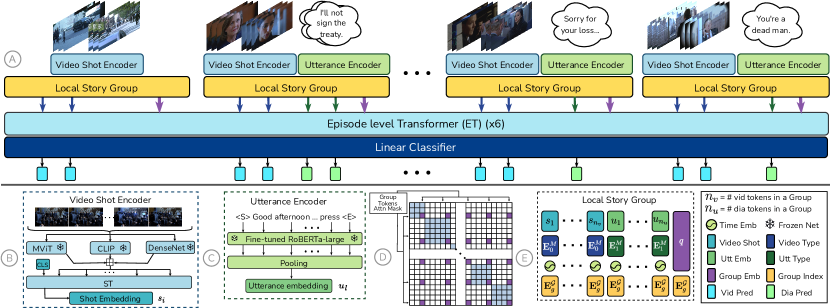
Figure 2: (A) TaleSumm ingests all video shots and dialogs of the episode and encodes them using (B) and (C). Based on temporal order, we combine tokens into local story groups (illustration shows small groups of 2 shots and 0-2 utterances). To each group, we append a group token and add multiple embeddings, before feeding them to the the episode-level Transformer ($\mathsf{ET}$). For each shot or dialog token, a linear classifier predicts its importance. (B) Video shot encoder. For each frame, representations from multiple backbones are fused using attention ($\boxplus$). We feed these to a shot Transformer encoder $\mathsf{ST}$, and tap a shot-level representation from the $\mathsf{CLS}$ token. (C) Utterance encoder uses a fine-tuned language model and avg-pooling across all words of the utterance. (D) Self-attention mask illustrates the block-diagonal self-attention structure across the episode. Group tokens across the episode (purple squares) communicate with each other. (E) Multiple embeddings are added to the tokens to capture modality type, time, and membership to a local story group.

We introduce TaleSumm, a two-level hierarchical model that identifies important sub-stories in a TV episode’s narrative (illustrated in Fig. 2). At the first level, our approach exploits frame-level (word-level) interactions to extract shot (dialog) representations (Sec. 4.2, Fig. 2(B, C)). At the second level, we capture cross-modal interactions across the entire episode through a Transformer encoder (Sec. 4.3, Fig. 2(A, D)). Before diving into the architecture, we formalize story summarization and introduce notation.

4.1 Problem Statement

Our aim is to extract a multimodal story summary (video and text) from a given episode, typically lasting around 40 minutes, and encompassing multiple key events.

Notation.

An episode $\mathcal{E}=(\mathcal{S},\mathcal{U})$ consists of a set of $N$ video shots $\mathcal{S}=\{s_{i}\}_{i=1}^{N}$ and a set of dialog utterances $\mathcal{U}=\{u_{l}\}_{l=1}^{M}$. A shot serves as a basic unit of video processing and comprises temporally contiguous frames taken from the same camera, while a dialog utterance typically refers to a sentence uttered by an individual as part of a larger conversation. We denote each shot as $s_{i}=\{f_{ij}\}_{j=1}^{T_{i}}$, where $f_{ij}$ are sub-sampled frames, and each utterance as $u_{l}=\{w_{lp}\}_{p=1}^{T_{l}}$ with multiple word tokens $w_{lp}$.

Summarization as importance scoring.

While humans may naturally select start and end temporal boundaries to indicate important sub-stories, for ease of computation, we discretize time and associate an importance score with each video shot or dialog utterance. Thus, given an episode $\mathcal{E}=(\mathcal{S},\mathcal{U})$, we formulate story summarization as a binary classification task applied to each element (shot or dialog). The ground-truth labels can be denoted as $\mathbf{y}^{\mathcal{S}}=\{y_{i}^{\mathcal{S}}\}_{i=1}^{N}$ and $\mathbf{y}^{\mathcal{U}}=\{y_{l}^{\mathcal{U}}\}_{l=1}^{M}$, where each $y_{i}^{\mathcal{S}},y_{l}^{\mathcal{U}}\in[0,1]$, signaling their importance to the story summary.

4.2 Level 1: Shot and Dialog Representations

In narrative video production, shots play an important role in advancing the storyline and contextualizing neighboring content. We obtain shot-level representations from granular frame-level features to determine how well the shot can contribute to understanding the storyline.

Feature extraction.

To capture various aspects of the shot, we use three pretrained backbones that capture visual diversity through people, their actions, objects, places, and scenes: $\phi_{\mathcal{S}}^{k}(\cdot),k=\{1,2,3\}$. We extract relevant visual information from frame(s) of a given shot, $s_{i}$ as follows:

$$\mathbf{f}_{ij}^{k}=\phi_{\mathcal{S}}^{k}\left(\{f_{ij}\}\right)\,,\quad\mathbf{f}_{ij}^{k}\in\mathbb{R}^{D_{\mathcal{S}}^{k}}.$$ (1)

Note that the backbone may encode a single frame $f_{ij}$ or a short sequence around $f_{ij}$.

For dialog utterances, we adopt a fine-tuned language model $\phi_{\mathcal{U}}^{\text{FT}}$, to compute contextual word-level features:

$$\mathbf{w}_{lp}=\phi_{\mathcal{U}}^{\text{FT}}\left(\{w_{lp}\}\right)\,,\quad\mathbf{w}_{lp}\in\mathbb{R}^{D_{\mathcal{U}}}\,.$$ (2)

Shot $\mathsf{CLS}$ pooling.

To compute an aggregated shot representation, we combine frame-level signals into a compact representation. An attention-based aggregation ($\boxplus$) (inspired by [32]), effectively weighs the most pertinent information (e.g. action in a motion-heavy shot or scenery in an establishing shot). First, the frame features from different backbones are projected to the same space (using $\mathbf{W}_{\mathcal{S}}^{k}{\in}\ \mathbb{R}^{D\times D_{\mathcal{S}}^{k}}$) and then concatenated to form $\hat{\mathbf{f}}_{ij}^{1:3}\in\mathbb{R}^{3D}$ (Eq. 3). A linear layer $\mathbf{W}_{\mathcal{P}}\in\mathbb{R}^{3\times 3D}$ followed by $\tanh$ and $\mathsf{softmax}$ computes scalar importance scores that are used for weighted fusion:

$$\hat{\mathbf{f}}_{ij}^{1:3} =[W_{\mathcal{S}}^{1}\mathbf{f}_{ij}^{1},W_{\mathcal{S}}^{2}\mathbf{f}_{ij}^{2},W_{\mathcal{S}}^{3}\mathbf{f}_{ij}^{3}]\,,$$ (3)

$$\boldsymbol{\alpha}_{ij}^{1:3} =\mathsf{softmax}(\tanh(W_{\mathcal{P}}\hat{\mathbf{f}}_{ij}^{1:3}))\,,$$ (4)

$$\mathbf{F}_{ij} =\alpha_{ij}^{1}\hat{\mathbf{f}}_{ij}^{1}+\alpha_{ij}^{2}\hat{\mathbf{f}}_{ij}^{2}+\alpha_{ij}^{3}\hat{\mathbf{f}}_{ij}^{3}\,.$$ (5)

We omit bias for brevity. We add relative frame position to $\mathbf{F}_{ij}$ through a time-embedding vector, $\mathbf{E}_{j}^{\mathcal{S}}$, similar to Fourier position encoding [104].

A shot transformer [104] $\mathsf{ST}$ is used to encode the frame-level feature sequence $\{\mathbf{F}_{ij}\}_{j=1}^{T_{i}}$. We tap the output from the $\mathsf{CLS}$ token appended at the beginning of the sequence (e.g. similar to BERT [15]) as the final shot representation:

$$\mathbf{s}_{i}=\mathsf{ST}(\{\mathbf{F}_{ij}+\mathbf{E}_{j}^{\mathcal{S}}\}_{j=1}^{T_{i}})\,,\quad\mathbf{s}_{i}\in\mathbb{R}^{D}\,.$$ (6)

Dialog utterance representation.

First, we project the tokens $\mathbf{w}_{lp}$ to $\mathbb{R}^{D}$ using a linear layer $\mathbf{W}_{\mathcal{U}}\in\mathbb{R}^{D\times D_{\mathcal{U}}}$. As the tokens are already contextualized by $\phi_{\mathcal{U}}^{\text{FT}}$, a simple mean-pool across the $p$ tokens is found to work well:

$$\mathbf{u}_{l}=\text{mean}_{p}(\{\mathbf{W}_{\mathcal{U}}\mathbf{w}_{lp}\}_{p=1}^{T_{l}})\,,\quad\mathbf{u}_{l}\in\mathbb{R}^{D}\,.$$ (7)

4.3 Level 2: Episode-level Interactions

We propose an episode-level Transformer encoder, $\mathsf{ET}$, that models interactions across shots and dialog of the entire episode. Predicting the importance of an element (shot or dialog) requires context in a neighborhood; e.g. shot in a scene, dialog utterance in a conversation.

Additional embeddings.

We arrange shot and dialog tokens based on their order in the episode (see Fig. 2(A)). Learnable type embeddings help the model distinguish between shot and dialog modalities ($\mathbf{E}^{M}\in\mathbb{R}^{2\times D}$). We encode the real time (in seconds) of appearance of each element (shot or dialog) using a binning strategy. Given an episode of $T$ seconds, we initialize Fourier position encodings $\mathbf{E}^{T}\in\mathbb{R}^{\lceil T/\tau\rceil\times D}$ where $\tau$ is the bin-size. Based on the mid-timestamp of each element $t$, we add $\mathbf{E}_{t}^{T}$ to the representation, the $\lfloor t/\tau\rfloor^{\text{th}}$ row in the position encoding matrix. Such time embeddings allow our model to: (i) implicitly encode shot duration; and (ii) relate co-occurring dialogs with video shots without the need for complex attention maps.

Local story groups.

The total number of video shots and dialog that make up the sequence length for $\mathsf{ET}$ is $S{=}N{+}M$ ($\sim$1500). Self-attention over so many tokens is not only computationally demanding, but also difficult to train due to unrelated temporally distant tokens that happen to look similar. We adopt a block-diagonal attention mask to constrain the tokens to attend to local story regions:

$$\mathbf{A}_{S\times S}=\text{diag}(\mathbbm{1}_{n_{1}\times n_{1}},\ldots,\mathbbm{1}_{n_{g}\times n_{g}},\ldots,\mathbbm{1}_{n_{G}\times n_{G}})\,,$$ (8)

where $\mathbbm{1}_{n_{g}\times n_{g}}$ denotes an all one matrix, $n_{g}$ is the # of tokens in the $g^{\text{th}}$ local block, $\sum_{g=1}^{G}n_{g}=S$, and $\text{diag}(\ldots)$ constructs a block diagonal matrix. We add new learnable group index embeddings $\mathbf{E}^{\mathcal{G}}\in\mathbb{R}^{G\times D}$ to our tokens to inform our model about their group membership.

Group tokens.

While capturing interactions across all tokens may lead to poor performance, self-attention only within the local story groups prohibits the model from capturing long-range story dependencies. To enable story group interactions, we propose to add a set of group tokens to the input, extending the sequence length to $\hat{S}{=}S{+}G$. The group tokens $\mathbf{q}_{g}$ represent an additional layer of hierarchy within the episode model as they summarize the story content inside a group and also communicate across groups, providing a way to understand the continuity of the story. Fig. 2(E) shows how group tokens are inserted at the end of each local story group’s shot and dialog tokens.

To facilitate cross-group communication, we make two modifications to the self-attention mask: (i) The size of each local group $n_{g}$ is extended by 1 to incorporate the group token $\mathbf{q}_{g}$ within the block matrix. We also update $\mathbf{A}$ to reflect this and is of size $\hat{S}\times\hat{S}$. (ii) We compute a binary index $\mathbf{o}\in\{0,1\}^{\hat{S}}$ to represent the locations at which a group token appears in the sequence. The new self-attention mask $\hat{\mathbf{A}}=\mathbf{A}+\mathbf{o}\mathbf{o}^{T}$ allows group-tokens to communicate. Fig. 2(D) illustrates the attention mask; light blue squares correspond to attention within a group, and sparse purple squares visualize attention across the group tokens.

Importance prediction.

We present how shot or dialog scores can be estimated. First, the input tokens to $\mathsf{ET}$ are:

$$\hat{\mathbf{s}}_{i} = \mathbf{s}_{i}+\mathbf{E}^{M}_{0}+\mathbf{E}^{T}_{t_{i}}+\mathbf{E}^{\mathcal{G}}_{g_{i}}\,,$$ (9)

$$\hat{\mathbf{u}}_{l} = \mathbf{u}_{l}+\mathbf{E}^{M}_{1}+\mathbf{E}^{T}_{t_{l}}+\mathbf{E}^{\mathcal{G}}_{g_{l}}\,,$$ (10)

$$\mathbf{q}_{g} = \mathbf{q}+\mathbf{E}^{\mathcal{G}}_{g}\,.$$ (11)

where $t_{i},t_{l}$ and $g_{i},g_{l}$ correspond to the mid-timestamp and group membership of shot $s_{i}$ and dialog $u_{l}$ respectively. $\mathbf{q}$ denotes the learnable shared group type embedding.

We feed the updated shot, dialog, and group token representations to $\mathsf{ET}$ post LayerNorm [8], a $H_{\mathsf{E}}$ layer Transformer encoder with a curated self-attention mask $\hat{\mathbf{A}}$:

$$[\ldots,\tilde{\mathbf{s}}_{i},\tilde{\mathbf{u}}_{l},\tilde{\mathbf{q}}_{g},\ldots]=\mathsf{ET}([\ldots,\hat{\mathbf{s}}_{i},\hat{\mathbf{u}}_{l},\mathbf{q}_{g},\ldots];\hat{\mathbf{A}})\,,$$ (12)

with all tokens, i.e. $\{i\}_{1}^{N}$, $\{l\}_{1}^{M}$, and $\{g\}_{1}^{G}$.

After $\mathsf{ET}$, we compute shot and dialog importance scores using a shared linear classifier $\mathbf{W}^{C}\in\mathbb{R}^{1\times D}$ followed by sigmoid function $\sigma(\cdot)$:

$$\hat{y}^{\mathcal{S}}_{i}=\sigma(\mathbf{W}^{C}\tilde{\mathbf{s}}_{i})\,\text{ and }\,\hat{y}^{\mathcal{U}}_{l}=\sigma(\mathbf{W}^{C}\tilde{\mathbf{u}}_{l})\,\forall i,l\,.$$ (13)

4.4 Training and Inference

Training.

TaleSumm is trained in an end-to-end fashion with BinaryCrossEntropy ($\mathsf{BCE}$) loss. We provide positive weights, $w$ (ratio of negatives to positives) to account for class imbalance. Modality specific losses are added:

$$\mathcal{L}=\mathsf{BCE}\left(\hat{\mathbf{y}}^{\mathcal{S}},\mathbf{y}^{\mathcal{S}};w^{\mathcal{S}}\right)+\mathsf{BCE}\left(\hat{\mathbf{y}}^{\mathcal{U}},\mathbf{y}^{\mathcal{U}};w^{\mathcal{U}}\right)\,.$$ (14)

Inference.

At test time, we follow the procedure outlined in Sec. 4.3 and generate importance scores for each video shot and dialog utterance (Eq. 13).

Model ablations.

As we will see empirically, our model is versatile and well-suited for adding/removing modalities or additional representations by adjusting the sequence length of the Transformer (number of tokens). It can also be modified to act as an unimodal model that applies only to video or dialog utterances by disregarding other modalities.

5 Experiments and Analysis

We first discuss the experimental setup.

Data splits.

We adopt 3 settings. (i) IntraCVT: On 24, most experiments (Tabs. 3, 4 and 5) follow an intra-season 5-fold cross-validation-test strategy. (ii) X-Season: On 24, we assess cross-season generalization using a 7-fold cross-validation-test (Tab. 7). (iii) X-Series: shows transfer results from 24 to PB (Tab. 7). More details can be found in Section A.3.

Evaluation metric.

We adopt Average Precision (AP, area under PR curve) as the metric to compare predicted importance scores of shots or dialogs against ground-truth.

5.1 Implementation details

We present some high-level details here.

Feature backbones.

We adopt three visual backbones: DenseNet169 [34] for object understanding; MViT [16] for action information; and OpenAI CLIP [78] for semantics.

To encode dialog, we adapt RoBERTa-large [123] for extractive summarization using parameter-efficient fine-tuning [33, 68] on the text from our dataset. The backbone is frozen when training TaleSumm for story summarization.

Additional backbone details are in Sections B.1 and B.2.

Architecture.

We find $H_{\mathsf{S}}{=}1$, $H_{\mathsf{E}}{=}6$, and $n_{g}{=}20$ to work best. Both $\mathsf{ST}$ and $\mathsf{ET}$ have the same configuration: 8 attention heads and $D{=}128$. We tried several architecture configurations whose details can be found at Section B.1.

Training details.

We randomly sample up to 25 frames per shot during training as a form of data augmentation and use uniform sampling during inference. Our model is implemented in PyTorch [74], has 1.94 M parameters, and is trained on 4 RTX-2080 Ti GPUs for a batch size of 4 (i.e. 4 entire episodes). The optimizer, learning rate, dropout, and other hyperparameters are tuned for best performance on the validation set and indicated in Section B.1.

5.2 Experiments on 24

	Video-only					Dialog-only
	Avg	Max	Cat	Tok	$\boxplus$	Max	Avg	wCLS
MLP	42.3	42.3	42.3	42.4	42.5	35.7	35.7	35.8
woG + FA	51.8	51.9	51.1	51.6	52.0	44.5	44.5	44.6
wG + SA	52.4	52.5	53.3	53.3	53.4	46.5	46.5	47.2

Table 3: Rows demonstrate methods for capturing episode-level interactions. In an MLP, tokens are independent. woG+FA is a Transformer encoder that captures full-attention over the entire episode without grouping; and wG+SA uses the proposed architecture with local story groups and sparse-attention. Columns describe the aggregation method used to combine frame (or token) level features into shot (or utterance) representation. C1 and C7 use average pooling. C2 and C6 use max pooling. C3-C5 are variants of $\mathsf{ST}$: C3 concatenates backbone features of each frame, C4 uses backbone features as separate tokens, and C5 uses proposed $\boxplus$ attention fusion. C8 uses the CLS token for dialog. Chosen: $\boxplus$ for shot, and average pooling for utterance representation.

Architecture ablations.

Results in Tab. 3 are across two dimensions: (i) columns span the shot or utterance level and (ii) rows span the episode level. All model variants outperform a baseline that predicts a random score between $[0,1]$: AP 34.2 (video) and 30.4 (dialog), over 1000 trials.

Across rows, we observe that the MLP performs worse than the other two variants by almost 10% AP score because assuming independence between story elements is bad. Our proposed approach with local story groups and sparse-attention (wG+SA) outperforms a vanilla encoder without groups and full-attention (woG+FA) by 1-2% on the video model and 2-3% for the dialog model.

Across columns, performance changes are minor. However, when using wG+SA at the episode-level, gated attention fusion with a shot transformer ($\boxplus$) improves results over Avg and Max pooling by 1%. For dialog-only, though wCLS outperforms Avg and Max by 0.7%, we adopt Avg pooling for its effective performance in a multimodal setup.

	Model	AttnMask	GToken	Video AP	Dialog AP
1	Video-only	SA	✓	53.4 $\pm$ 3.9	-
2	Dialog-only	SA	✓	-	47.2 $\pm$ 3.9
3	TaleSumm	FA	-	51.8 $\pm$ 3.6	43.8 $\pm$ 4.7
4		FA	✓	51.9 $\pm$ 3.7	44.0 $\pm$ 4.6
5		SA	-	53.9 $\pm$ 3.4	48.8 $\pm$ 4.6
6		SA	✓	54.2 $\pm$ 3.3	49.0 $\pm$ 4.9

Table 4: TaleSumm ablations. The AttnMask column indicates if the self-attention mask is applied over the full episode (FA) or uses sparse block diagonal structure of story groups (SA). The GToken indicates whether the group token is absent (-) or present (✓). R6 is our final chosen model for subsequent experiments.

TaleSumm ablations

are presented in Tab. 4. Rows 1 and 2 highlight the best video-only and dialog-only models (from Tab. 3). We report mean $\pm$ std dev on the val set. Std dev is found to be high due to variation across multiple folds; but low across random seeds. Results for joint prediction of video shot and utterance importance are shown in rows 3-6. Our proposed approach in row 6 performs best for both modalities, outperforming rows 3-5.

Model	Val		Test
	Video AP	Dialog AP	Video AP	Dialog AP
PGLSUM [6]	48.8 $\pm$ 3.3	-	47.1 $\pm$ 2.4	-
MSVA [20]	47.3 $\pm$ 3.8	-	45.5 $\pm$ 1.2	-
Video-Only	53.4 $\pm$ 3.9	-	50.6 $\pm$ 3.6	-
PreSumm [56]	-	43.1 $\pm$ 3.3	-	41.6 $\pm$ 2.0
Dialog-Only	-	47.2 $\pm$ 3.9	-	43.4 $\pm$ 2.8
A2Summ [28]	35.1 $\pm$ 1.8	33.2 $\pm$ 2.8	33.8 $\pm$ 1.7	31.6 $\pm$ 2.2
TaleSumm (Ours)	54.2 $\pm$ 3.3	49.0 $\pm$ 4.9	50.1 $\pm$ 2.8	46.0 $\pm$ 2.1

Table 5: Comparison against SoTA video-only, text-only, and multimodal summarization models. Our approach outperforms previous work by a significant margin.

SoTA comparison.

We compare against SoTA methods: (i) video-only (PGLSUM [6], MSVA [20]), (ii) dialog-only (PreSumm [56]), and (iii) multimodal (A2Summ [28]) in Tab. 5. While none of the above methods are built for processing 40 minutes of video, we make modifications to them to make them comparable to our work (details in the supplement). On both the validation and the test set, TaleSumm outperforms all other baselines in both modalities.

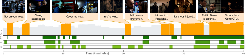
Figure 3: TaleSumm predictions on S06E22 of 24 (test set). “Ours” filled-plot illustrates the importance score profile over time, where orange patches indicate story segments selected for summarization. Annotations are shown below: ground-truth ( GT), fandom ( F), and human annotated ( H). The story: Amid the high-stakes sequence depicted in the selected groups 1-3, Zhou Yong’s team captures Josh Bauer, leading to a firefight with Jack Bauer, who seeks Josh’s location. Negotiations with Phillip Bauer over Josh’s return for a vital circuit board escalate global tensions between Russia and the USA. Simultaneously, Mike Doyle defies Jack’s wishes and departs with Josh by helicopter (segment 7). Parallely, Lisa, backed by Tom Lennox, confronts a Russian agent, leading to her injury (4, 6). Morris attempts to console Nadia for Milo’s loss at CTU in 5. Escalating global tensions and the imminent showdown mark the episode.

5.3 Analysis and Discussion

Model	SumMe			TVSum
	F1	SP	KT	F1	SP	KT
MSVA [20]	52.4	12.3	9.2	63.9	32.1	22.0
PGLSUM [6]	56.2	17.3	12.7	63.9	40.5	28.2
A2Summ [28]	54.0	3.5	2.8	62.9	25.2	17.1
TaleSumm (Ours)	57.5	23.8	17.6	64.0	26.7	18.2

Table 6: Comparison with SoTA methods on the SumMe [24] and TVSum [93] benchmark datasets. Metrics are suggested by Otani et al. [67]: F1, Kendall’s $\tau$ (KT), and Spearman’s $\rho$ (SP).

Video summarization benchmarks.

We evaluate TaleSumm on SumMe [24] and TVSum [93]. However, both datasets are small (25 and 50 videos) and have short duration videos (few minutes). As splits and metrics are not comparable across previous works, we re-ran the baselines.

While MSVA uses three feature sets: i3d-rgb, i3d-flow [10] and GoogleNet [96] with intermediate fusion, PGLSUM uses GoogleNet and captures local and global features. In contrast, A2Summ [28] aligns cross-modal information using dual-contrastive loss between video (GoogleNet features) and text (captions generated using GPT-2 [77], embedded by RoBERTa [123] at frame level).

Similar to MSVA, we fuse all 3 features. Even though TaleSumm is built for long videos (group blocks, sparse attention), Tab. 6 shows that we achieve SoTA on SumMe. The drop in performance on TVSum may be due to video diversity (documentaries, how-to videos, etc.).

		X-Season (24)		X-Series (PB)
	Model	Video	Dialog	Video	Dialog
1	MSVA [20]	46.7 $\pm$ 2.7	-	32.7	-
2	PGLSUM [6]	47.1 $\pm$ 2.4	-	34.5	-
3	PreSumm [56]	-	41.3 $\pm$ 3.2	-	38.3
4	A2Summ [28]	33.5 $\pm$ 3.2	31.7 $\pm$ 2.9	20.2	19.0
5	TaleSumm (Ours)	51.0 $\pm$ 4.6	46.0 $\pm$ 5.5	36.7	35.7

Table 7: We evaluate our model’s generalization across seasons within 24 and across TV shows (24 $\rightarrow$ Prison Break). R5 showcases superiority of our methods compared to SoTA. In X-Series, the random baseline achieves 21.3 and 19.1 for video and dialog.

Generalization to a new season/TV series.

Tab. 7 shows results in two different setups. In X-Season, we see the impact of evaluating on unseen seasons (in a 7-fold cross-val-test). While TaleSumm outperforms baselines, it is interesting that most methods show comparable performance across IntraCVT and X-Season setups (see Tabs. 7 and 5).

In the X-Series setting, we train our model on 24 and evaluate on Prison Break. Although both series are crime thrillers, there are significant visual and editing differences between the two shows. Our approach obtains good scores on video summarization, and is a close second on dialog.

Dataset	Cronbach $\alpha$		Pairwise $F_{1}$		Fleiss’ $\kappa$
	Video	Dialog	Video	Dialog	Video	Dialog
SumMe	0.88	-	0.31	-	0.21	-
TVSum	0.98	-	0.36	-	0.15	-
PlotSnap (Ours)	0.91	0.93	0.59	0.60	0.38	0.39

Table 8: Label consistency across datasets.

Methods	Fandom (F)		Human (H)
	Video AP	Dialog AP	Video AP	Dialog AP
GT	64.1	63.8	44.8	42.2
PGLSUM	43.0	-	47.6	-
MSVA	34.3	-	42.2	-
PreSumm	-	43.6	-	46.7
A2Summ	28.7	29.7	41.0	41.1
TaleSumm	44.5	45.5	48.7	50.9

Table 9: Results on labels from 24 fan site (F) and human-annotated story summaries (H) averaged over 17 episodes of 24.

Label consistency.

As suggested by [24, 93], label consistency is crucial to evaluate summarization methods. We assess PlotSnap using Cronbach’s $\alpha$, pairwise $F_{1}$-measure, and another agreement score: Fleiss’ $\kappa$.

We obtain three sets of labels for 17 episodes of 24 (details in Sec. A.4). (i) GT: obtained from matching recaps; (ii) F: maps plot events from a 24 fan site to videos; (iii) H: human response for a summary. Our labels have superior consistency compared to SumMe [24] and TVSum [93] (see Tab. 8), indicating that identifying key story events in a TV episode is less subjective than scoring importance for generic Youtube videos. Tab. 9 shows the results for the baselines and TaleSumm on the two other labels F and H. Our model predictions are better aligned with both labels.

Qualitative analysis.

We show the model’s predictions and compare against all three labels (GT, F, and H) for one episode in Fig. 3. Our model identifies many important story segments that are also part of the annotations.

6 Conclusion

Our work pioneered the use of TV episode recaps for story understanding. We proposed PlotSnap, a dataset of two TV shows with high-quality recaps, leveraging them for story summarization labels, while showing high consistency across labeling approaches. We introduced TaleSumm, a hierarchical summarization approach that captures and compresses shots and dialog, and enables cross-modal interactions across the entire episode, trainable on a single GPU of $12\text{\,}\mathrm{GB}$. We performed thorough ablations, established SoTA performance, and demonstrated transfer across seasons, other series, and even movie genres. For reproducibility and encouraging future work, we will release the code and share the dataset, as keyframes, features, and labels.

Limitations and future work.

While our current work focuses on recaps obtained from a limited genre and two TV series, we believe the approach should be scalable to additional genres and datasets. Early experiments in evaluating our model on condensed movies (CMD) [9] show limited improvements. Our approach to story summarization does not explicitly model the presence of characters (e.g. via person and face tracks and their emotions [94]) which are central to any story and this can be an important direction for future work. Additional discussions are provided in the supplementary material.

Acknowledgments.

We thank the Bank of Baroda for partial travel support, and IIIT-H’s faculty seed grant and Adobe Research India for funding. Special thanks to Varun Gupta for assisting with experiments and the Katha-AI group members for user studies.

Appendix

We provide additional information and experimental results to complement the main paper submission. In this work, we propose a dataset PlotSnap consisting of two crime thriller TV shows with rich recaps and a new hierarchical model TaleSumm that selects important local story groups to form a representative story summary. We present details of PlotSnap in App. A. App. B extends on additional experimentation on PlotSnap as well as SumMe [24] and TVSum [93] followed by an extensive qualitative study. Finally, we conclude this supplement with a discussion of future research directions in App. C.

Appendix A Dataset Details

We start with the essential step of creating soft labels for each shot and dialog of the episode, presented in Sec. A.1. We describe how recaps are used to generate binary labels using our novel shot-matching algorithm. Next, Sec. A.2 describes how label smoothing is performed. This is an essential step towards capturing the local sub-story in a better way. Further, Sec. A.3 comments on the different data split creation strategies used to evaluate baselines and our model’s generalizability. Finally, to conclude Sec. A.4 presents detailed episode-level label reliability scores.

A.1 Shot Matching

We propose a novel shot-matching algorithm whose working principle involves frame-level similarities to obtain matches.

First, we compute frame-level embeddings using DenseNet169 [34], which were found to work better than models such as ResNet pre-trained on ImageNet [84, 29] based on a qualitative analysis. An example is shown in Fig. 4 where we see higher similarity between retrieved episode frames and the query frame from the recap.

Second, we discuss how these embeddings are used to obtain matches is detailed below.

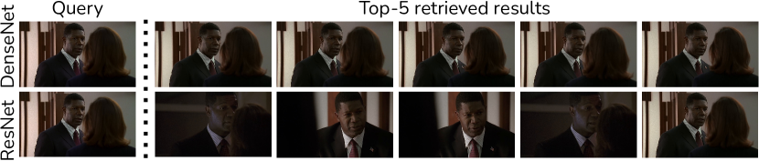
Figure 4: Retrieval results for Recap from Episode Frames with DenseNet (Top) v/s ResNet (bottom). We observe qualitatively that DenseNet is able to match to the correct frames from the episode more often.

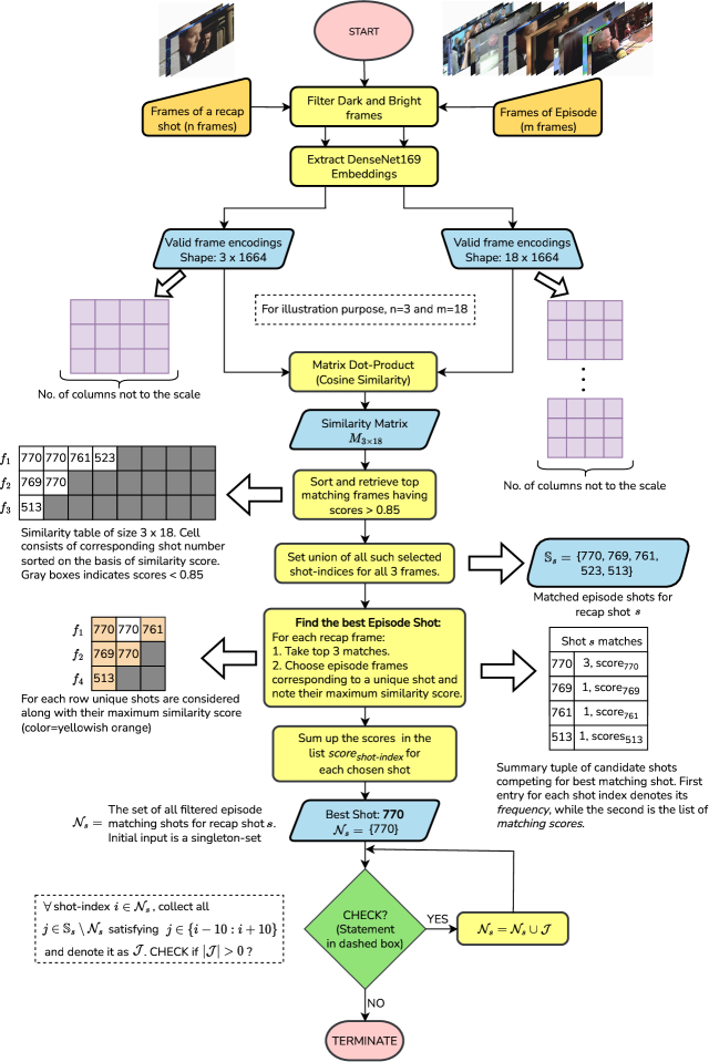
Figure 5: Flowchart for identifying shots from the episode that appear in a recap and can be used as weak labels for story summarization. The process involves identifying the list of high-scoring matching frames, indexing the shots, and then preventing spurious matches by looking for high-scoring matches within a bounded duration. The flowchart presents an example of the process used to identify the set of shots $\mathcal{N}_{s}$ from the episode that match to the recap shot.

Matching.

For a given recap shot $s$ in $\mathcal{R}_{n+1}$ we compare it against multiple frames in the episode $\mathcal{E}_{n}$, and compute a matrix dot-product with appropriate normalization (cosine similarity) between respective frame representations of the recap and episode as illustrated in the toy-example of Fig. 5. We remove very dark or very bright frames, typical in poor lighting conditions or glares, to avoid spurious matches and noisy labels.

Next, we choose a high threshold to identify matching frames ($0.85$ in our case after analysis) and fetch all the top matching frames along with their shot indices (the shot where the frame is sourced from). We compute a set union over all matched shots obtained by scoring similarities between the recap frame of shot $s$ and denote this set as $\mathbb{S}_{s}$. In the example, we match 3 frames of a recap shot and identify several episode shots shown in the blue box with $\mathbb{S}_{s}$.

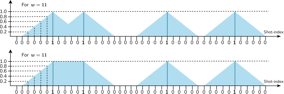
Figure 6: Triangle smoothing process. Here x-axis denotes binary labels derived from the shot matching process, while y-axis shows soft importance scores used to train our model. Top: The triangular filter is applied at each shot selected from the matching process. Scores of shots falling within the window are updated. Bottom: In the second step, we add shot importance derived potentially from multiple overlapping triangle filters. This typically happens when episode shots in close proximity are matched to the recap.

Weeding out spurious shot matches.

The set $\mathbb{S}_{s}$ may contain shots beyond a typical shot thread pattern due to spurious matches. These need to be removed to prevent wrong importance scores from being obtained from the recap. To do this, we first find the best matching shot in the episode. We observe that taking top three matched frames for every recap frame results in strong matches. Subsequently, we pick the maximum similarity score for each unique shot matched to a recap frame. This allows us to accumulate the score for an episode shot if multiple frames of the episode shot match with frames of the recap shot. The shot that scores the highest (after summing up the scores) is considered the best-matched episode shot for recap shot $s$.

Next, we choose a window size of 21 (10 on either side) and include all shots in $\mathbb{S}_{s}$ that fall within this window to a new matched set, $\mathcal{N}_{s}$. This is motivated by the typical duration of a scene in a movie or TV episode (40-60 seconds) and an average shot duration of 2-3 seconds. We repeat this process until no more shots are added to the set $\mathcal{N}_{s}$ and discard the rest in $\mathbb{S}_{s}$. Thus, for a given shot from the recap, we obtain all matching shots in the episode that are localized to a certain region of high-scoring similarity (see Fig. 5). We repeat this process for all frames and shots from the recap.

A.2 Label Smoothing

The intuition behind extending the recap matched shots obtained in the previous section is to include chunks of the sub-story that are important to the storyline. While a short recap (intended to bring back memories) only selects a few shots, a story summary should present the larger sub-story. Selecting only one shot in a thread [99] also adversely affects model training due to conflicting signals, as multiple shots with similar appearance can have opposite labels. Label smoothing solves both these issues.

Triangle Smoother.

We hypothesize that the importance of shots neighboring a matched shot are usually quite high and use a simple triangle smoother to re-label the importance of shots. In particular, we slide a window of size $w$ centering at positive labels and set the importance of neighboring shots according to height of the triangle. The above process is illustrated in Fig. 6 as the first step. In the second step, we add and clip the soft labels of strongly overlapping regions to prevent any score from going higher than 1. For the sake of simplicity, we used triangle smoothing, however, one could also use other filters.

We choose $w=17$ by analyzing the spread of the shots and their importance scores and comparing them against a few episodes for which we manually annotated the story summaries.

Dialog labels.

The above smoothing procedure generates soft labels for video shots. For dialog utterances, we simply import the score of the shot that encompasses the mid-timestamp of the dialog. The key assumption here is that the dialog utterance associated with the matched shot is also important.

A.3 Data Splits

For evaluation of our approach, PlotSnap is split into 4 types of splits as described below:

1. IntraCVT (Intra-Season 5 fold cross-val-test) represents 5 different non-overlapping splits from 7 seasons of 24 (Season 2 to 8). Intra-season means episodes from each season are present in the train/val/test splits. For example, split-1 uses 5 episodes from the end of each season for val and test (2, 3 respectively). Likewise, Split-5 (the fifth fold) uses episodes from the beginning of the season in val/test. We observe that Split-5 is harder.

2. X-Season (Cross-Season 7 fold cross-val-test) involves 7 non-overlapping splits with one season entirely kept for testing (from Season 2 to 8), while the train and val use 18 and 5 episodes respectively from each season. This strategy is used to test for the generalization of our model on different seasons of the same series, 24.

3. X-Series (Cross-Series) split includes 8 seasons (seasons 2 to 9) from 24in train/val (19/4) and 2 seasons (seasons 2 and 3) from PB for the test. This split is designed to check the effectiveness of our model across TV series.

4. Multiple labels split consists of a single non-overlapping train/val/test split with 126/18/17 episodes from 24, respectively. We collect story summary annotations from 3 sources for the test set (recap: GT, fan website: F, and human annotation: H). This split is used for comparison against labels from Fandom or Human annotations.

A.4 Label Consistency

As discussed in Tab. 8 (of the main paper), we show the agreement between story summary labels obtained from different sources. Consistency is evaluated on 3 kinds of labels: From recap (GT), Fandom (F) and Human (H). We assess the consistency of labels via Cronbach’s $\alpha$, Pairwise $F_{1}$, and Fleiss’ $\kappa$ statistics.

Tab. 10 expands on the individual scores obtained for each of the 17 episodes. We observe that Cronbach’s $\alpha$ is consistently high, while Fleiss’s $\kappa$ varies typically between 0.2-0.5 indicating fair to moderate agreement.

season	episode	Video			Dialog
		C$\alpha$	P$F_{1}$	F$\kappa$	C$\alpha$	P$F_{1}$	F$\kappa$
S02	E21	0.978	0.51	0.337	0.964	0.51	0.335
S02	E23	0.937	0.407	0.135	0.966	0.472	0.182
S03	E20	0.959	0.684	0.595	0.939	0.715	0.629
S03	E22	0.907	0.568	0.422	0.861	0.553	0.409
S04	E20	0.954	0.671	0.47	0.949	0.716	0.568
S04	E21	0.981	0.618	0.405	0.983	0.504	0.286
S05	E21	0.886	0.521	0.27	0.872	0.497	0.249
S05	E22	0.994	0.573	0.282	0.991	0.611	0.334
S06	E20	0.986	0.639	0.432	0.975	0.689	0.534
S06	E21	0.979	0.645	0.437	0.96	0.618	0.439
S06	E22	0.965	0.557	0.297	0.929	0.632	0.406
S06	E23	0.981	0.496	0.263	0.986	0.475	0.206
S07	E20	0.942	0.684	0.451	0.968	0.67	0.382
S07	E22	0.849	0.531	0.349	0.892	0.54	0.334
S07	E23	0.993	0.525	0.215	0.988	0.541	0.235
S08	E21	0.233	0.68	0.527	0.715	0.667	0.518
S08	E22	0.968	0.685	0.507	0.948	0.728	0.538
Average		0.911	0.588	0.376	0.934	0.596	0.387

Table 10: Detailed overview of reliability scores for 17 episodes from 24 (test set of multiple labels split) with the last row showing the average across all episodes. Si and Ej stands for Season i Episode j, C$\alpha$ for Cronbach’s $\alpha$, P$F_{1}$ for Pairwise $F_{1}$, and F$\kappa$ for Fleiss’ $\kappa$.

Appendix B Experiments and Results

In this section we expand our implementation details (Sec. B.1) and present additional details of the backbones used for feature extraction (Sec. B.2). Extensive ablation studies with regard to feature combinations and model hyperparameters are presented in Sec. B.3.

In Sec. B.4, we present details of the modifications that need to be made to adapt SoTA baselines such as MSVA [20], PGL-SUM [6], PreSumm [56], and A2Summ [28] for comparison with TaleSumm. Sec. B.5 details how we adapted our model for SumMe and TVSum, along with comprehensive hyperparameter particulars. To conclude, Sec. B.6 shows extended qualitative analysis, as in the main paper, on three other episodes (S06E20, S07E22, and S05E21).

B.1 Implementation Details

Visual features.

We first segment the episode into shots using [109]. We adopt 3 specialized backbones (for their combined effective performance; shown in Tab. 11): (i) DenseNet169 [34] pre-trained on ImageNet [84], SVHN [110], and CIFAR [47] for object semantics; (ii) MViT [16] pre-trained on Kinetics-400 [40] for action information; and (iii) OpenAI CLIP [78], pre-trained on 4M image-text pairs, for semantic information.

Utterance features

. We adapt RoBERTa-large [123] originally pretrained on the reunion of five datasets: (i) BookCorpus [121], a dataset consisting of 11,038 unpublished books; (ii) English Wikipedia [5] (excluding lists, tables and headers); (iii) CC-News [3], a dataset containing 63 millions English news articles crawled between September 2016 and February 2019; (iv) OpenWebText [4], an opensource recreation of the WebText dataset used to train GPT-2; and (v) Stories [103] a dataset containing a subset of CommonCrawl data filtered to match the story-like style of Winograd schemas [52]. Together these datasets weigh 160GB of text.

Given dialogs from the episode, our fine-tuning objective is to predict the important dialogs. We extract word/token-level representations ($\mathbf{w}$) from finetuned (but frozen) RoBERTa-large ($\phi_{\mathcal{U}}^{\text{FT}}$) for the task of dialog story summarization.

Frame sampling strategy.

We randomly sample up to 25 frames per shot during training as a form of data augmentation. During inference, we use uniform sampling. We used fourier position embeddings $\mathbf{E}^{\mathcal{S}}_{j}$ for indexing video frames.

Architecture details.

We experiment with the number of layers for $\mathsf{ST}$, $H_{\mathsf{S}}{\in}[1:3]$ and $\mathsf{ET}$, $H_{\mathsf{E}}{\in}[1:9]$, and find $H_{\mathsf{S}}{=}1$ and $H_{\mathsf{E}}{=}6$ to work best. Except the number of layers, $\mathsf{ST}$ and $\mathsf{ET}$ have the same configuration: 8 attention heads and $D{=}128$. Appropriate padding and masking is used to create batches. We compare multiple local story group sizes $n_{g}\in\{5:30:5\}$ and find $n_{g}{=}20$ to work best.

Training details.

Our model is trained on 4 RTX-2080 Ti GPUs for a maximum of 65 epochs with a batch size of 4 (i.e. 4 entire episodes – each GPU handling one episode). We adopt the AdamW optimizer [58] with parameters: learning rate${=}10^{-4}$, weight decay${=}10^{-3}$. We use OneCycleLR [91] as learning rate scheduler with max lr${=}10^{-3}$, and multiple dropouts [30]: $0.1$ for projection to 128 dim inside video and utterance encoder; $0.2$ for attention layers; and $0.2$ for the classification head. The hyperparameters are tuned for best performance on validation set.

B.2 Feature Extraction

Prior to feature extraction, setting an appropriate fps for every video is important to trade off between capturing all aspects of the video while keeping computational load low. We find 8 fps to be a good balance between the two.

Visual Feature Backbones

We present the details for three backbones capturing different aspects of a video.

DenseNet169

$\mathbf{f}^{1}$. Feature extraction of salient objects/person in each frame is of utmost priority and is achieved through DenseNet169 [34] pretrained on ImageNet [84], SVHN [110], and CIFAR [47]. We consider the frozen backbone without the linear classification head to obtain flattened features, $\mathbf{f}^{1}\in\mathbb{R}^{1664}$. Before feeding the images, we apply a few preprocessing steps to sub-sample raw images.

1. Frames are resized to $256{\times}256$ resolution along with center cropping.

2. RGB pixel values are scaled to $[0,1]$ followed by mean and standard deviation normalization.

We use the architecture as well as parameters from PyTorch Hub, version pytorch/vision:v0.10.0.

MVIT

$\mathbf{f}^{2}$. Beyond objects/person, their actions too affect the importance of a shot, and hence having them serves the purpose of representing a shot from a different perspective. For this, we use MViT [16] pretrained on Kinetics-400 [40]. We feed the original video with some pre-processing as explained above to obtain feature embeddings, $\mathbf{f}^{2}\in\mathbb{R}^{768}$. With a window-size${=}32$ and stride${=}16$, we extracted per-window encodings while padding zeros at the end (black-frames) to account for selecting window-size amount of frames.

1. Frame resizing to 256${\times}$256 followed by center-cropping to 224${\times}$224 resolution.

2. Pixel scaling from 8-bit format to float format ($[0,1]$). Following this, mean and standard deviation normalization is performed.

3. We chose MViT-Base $32{\times}3$ that ingests a chunk of video (32 frames) at once and produces an embedding vector.

We import the architecture and pretrained parameters from PytorchVideo.

CLIP

$\mathbf{f}^{3}$. This is a multi-modal backbone that can produce representations corresponding to matching textual descriptions. We borrow the CLIP [78] pre-trained model from the huggingface [106] library and use their inbuilt image processor as well as feature extractor to obtain subsampled frame-level encodings, $\mathbf{f}^{3}\in\mathbb{R}^{512}$.

1. Short-side is resized to 224 pixels followed by center-cropping (to $224{\times}224$).

2. Re-scaling 8-bit image to $[0,1]$ interval.

3. Mean and standard deviation normalization.

Dialog Features

We test three different dialog features and present the details as follows.

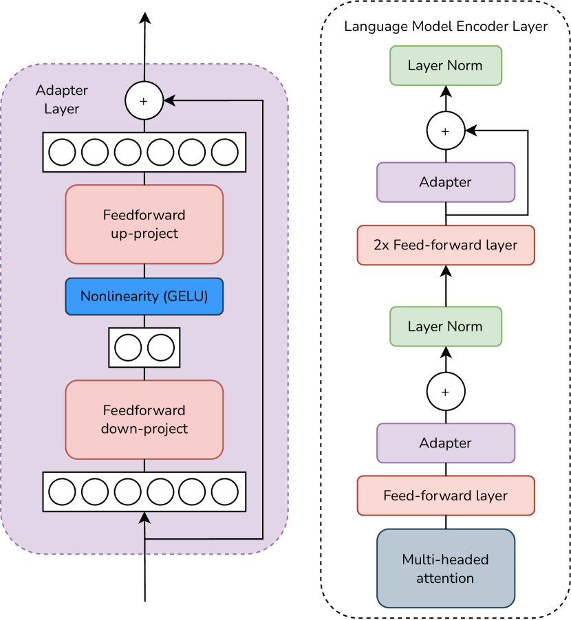
Figure 7: Architecture of the adapter module [33] and its integration with language model’s encoder layer. Left: The adapter module has fewer parameters compared to the attention and feedforward layers in a Transformer layer and consists of a bottleneck and skip-connection. Right: We add the adapter module twice to each encoder layer. Once after the multi-head attention and the other is placed after the two feed-forward layers typical of a Transformer architecture. For the Transformer decoder, in the case of PEGASUS${}_{\text{LARGE}}$, we add one extra adapter after cross-attention as well. Adaptation: When adapting the model, the purple and green layers illustrated on the right module are trained on the downstream data and task, while the other blocks are frozen.

Fine-tuning Language Models.

We fine-tune language models such as PEGASUS${}_{\text{LARGE}}$ [112], RoBERTa-Large [123], and MPNet-base-v2 [92] for our task of extractive dialog summarization. To account for the small dataset sizes, for all fine-tuning, we use the Adapter modules [33] that add only a few trainable parameters in the form of down- and up-projection layers as illustrated in Fig. 7.

RoBERTa-Large [123] and MPNet-base-v2 [92] are fine-tuned for utterance-level binary classification to decide whether the dialog utterance is important or not.

PEGASUS${}_{\text{LARGE}}$ is trained originally to generate abstractive summaries. Instead, we adapt it to generate summary dialogs. As the number of tokens accepted by the PEGASUS${}_{\text{LARGE}}$ model does not allow feeding all the dialog from the episode, we break it into 6 chunks.

Word-level embeddings.

We use last hidden-state of the encoder to obtain contextualized word-level embeddings, $\mathbf{w}\in\mathbb{R}^{1024}$ ($768$ for MPNet-base-v2). PEGASUS${}_{\text{LARGE}}$, being a generative model (consisting of both encoder and decoder), we keep only the encoder portion for word-level feature extraction.

B.3 Feature and Architecture Ablations

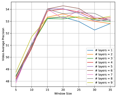
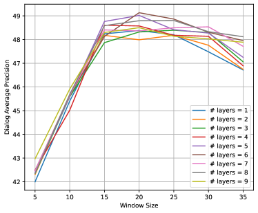
Figure 8: Performance of TaleSumm for varying local story group size (also referred to as window size) and number of layers in the episode-level Transformer $\mathsf{ET}$. y-axis denotes the AP score for the Left: Video and Right: Dialog. We observe that a 6 layer model $H_{\text{E}}=6$ works well together with a local story group size of $n_{g}=20$.

All experiments are run on IntraCVT split, and we report mean and standard deviation.

Pooling		Avg	Max	Cat	Tok	Stack	$\boxplus$
Concatenate		✓	✓	✓	NC	✓	✓
DMC	Vid AP	54.1 $\pm$ 4.5	54.1 $\pm$ 4.6	54.2 $\pm$ 4.1	54.1 $\pm$ 4.0	53.9 $\pm$ 4.7	54.2 $\pm$ 3.3
	Dlg AP	48.7 $\pm$ 4.1	48.8 $\pm$ 4.4	48.9 $\pm$ 4.7	49.0 $\pm$ 4.8	49.1 $\pm$ 4.8	49.0 $\pm$ 4.9
DM	Vid AP	54.0 $\pm$ 3.8	54.1 $\pm$ 3.3	54.0 $\pm$ 4.1	53.9 $\pm$ 3.2	53.6 $\pm$ 4.3	53.7 $\pm$ 3.0
	Dlg AP	48.6 $\pm$ 4.4	48.8 $\pm$ 4.4	48.9 $\pm$ 4.4	48.6 $\pm$ 3.6	48.4 $\pm$ 4.8	48.6 $\pm$ 4.3
MC	Vid AP	53.8 $\pm$ 3.6	53.9 $\pm$ 4.0	53.8 $\pm$ 4.5	54.0 $\pm$ 4.9	53.8 $\pm$ 4.2	54.2 $\pm$ 4.3
	Dlg AP	48.5 $\pm$ 4.6	48.8 $\pm$ 4.1	48.7 $\pm$ 4.5	49.0 $\pm$ 4.1	48.5 $\pm$ 4.7	49.1 $\pm$ 4.2
DC	Vid AP	54.0 $\pm$ 4.5	54.1 $\pm$ 4.3	54.1 $\pm$ 4.0	54.0 $\pm$ 4.0	54.1 $\pm$ 3.9	54.1 $\pm$ 4.2
	Dlg AP	48.2 $\pm$ 4.9	48.7 $\pm$ 4.5	48.9 $\pm$ 4.7	49.0 $\pm$ 4.6	49.0 $\pm$ 4.8	49.0 $\pm$ 4.9
D	Vid AP	53.5 $\pm$ 4.2	53.4 $\pm$ 4.2	54.0 $\pm$ 3.8	-	-	-
	Dlg AP	48.1 $\pm$ 4.2	48.6 $\pm$ 4.3	48.9 $\pm$ 4.4	-	-	-
M	Vid AP	52.9 $\pm$ 3.2	53.6 $\pm$ 3.6	53.5 $\pm$ 3.4	-	-	-
	Dlg AP	48.2 $\pm$ 4.0	48.4 $\pm$ 3.9	48.7 $\pm$ 4.6	-	-	-
C	Vid AP	53.9 $\pm$ 3.7	53.9 $\pm$ 3.9	54.1 $\pm$ 3.7	-	-	-
	Dlg AP	48.6 $\pm$ 4.2	48.7 $\pm$ 4.2	48.7 $\pm$ 4.0	-	-	-

Table 11: TaleSumm ablations for different feature combination strategies, using both video and dialog modalities. Feature ablations are performed over the visual modality. Columns describe the Pooling approaches used to form shot-level from frame-level representations; Concatenate corresponds to how backbone feature are combined (concatenate ✓ or as separate tokens (NC)). Stack pooling is an alternative approach to $\boxplus$, where instead of condensing the aggregated (concatenated) visual features via a linear layer $\mathbf{W}_{\mathcal{P}}\in\mathbb{R}^{3\times 3D}$, we obtain individual feature importance score (with $\mathbf{W}_{\mathcal{P}}\in\mathbb{R}^{1\times D}$ followed by $\tanh$ and $\mathsf{softmax}$). D: DenseNet169, M: MViT, and C: CLIP. All results are for TaleSumm that captures Episode level interactions.

Visual features for Story summarization.

Table 11 shows the results for all combinations of the three chosen visual feature backbones in a multimodal setup. We draw two main conclusions: (i) The Shot Transformer encoder ($\mathsf{ST}$) shows improvements when compared to simple average or max pooling. (ii) DMC (DenseNet + MViT + CLIP), the feature combination that uses all backbones, performs well, while MC shows on-par performance. Importantly, the feature combination is better than using any feature alone.

Pooling		Max	Avg	wCLS
PEGASUS${}_{\text{LARGE}}$ [112]	Vid AP	52.7 $\pm$ 4.3	53.1 $\pm$ 4.2	53.1 $\pm$ 4.7
	Dlg AP	47.9 $\pm$ 3.6	48.0 $\pm$ 5.1	47.9 $\pm$ 4.9
MPNet-Base [92]	Vid AP	53.2 $\pm$ 3.9	53.1 $\pm$ 3.7	53.5 $\pm$ 3.4
	Dlg AP	48.0 $\pm$ 4.4	47.2 $\pm$ 3.2	48.6 $\pm$ 5.0
RoBERTa-Large [123]	Vid AP	54.1 $\pm$ 3.8	54.2 $\pm$ 3.3	54.1 $\pm$ 4.2
	Dlg AP	49.0 $\pm$ 4.6	49.0 $\pm$ 4.9	49.0 $\pm$ 4.3

Table 12: TaleSumm ablations for various dialog utterance feature backbones. Visual features are fixed to DMC.

Language backbones for Story summarization.

Different from the previous experiment, Table 12 shows results for different dialog features with different word-to-utterance pooling approaches in a multimodal setting. RoBERTa-Large outperforms all other language models. Nevertheless, the other models are not too far behind.

Number of $\mathsf{ET}$ layers and local story group size.

Two important hyperparameters for our model are the number of layers $H_{\text{E}}$ in the $\mathsf{ET}$ and the local story group size $n_{g}$. Fig. 8 shows the performance on video AP (left) and dialog AP (right) with a clear indication that 6 layers and a story group size of 20 shots are appropriate.

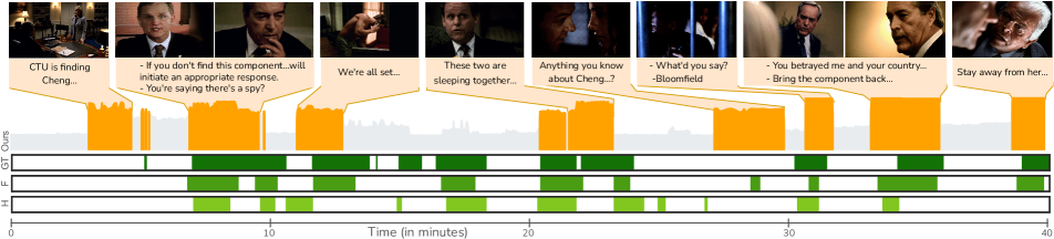
Figure 9: TaleSumm predictions on S06E20 of 24 (test set). “Ours” filled-plot illustrates the importance score profile over time, where orange patches indicate story segments selected for summarization. Annotations are shown below: ground-truth ( GT), fandom ( F), and human annotated ( H). We number the grouped frames representing the predicted contiguous orange chunks as shot groups (SG-n), e.g. this episode has 8 SGs. The story: The White House directs CTU to locate Cheng, as depicted in SG-1, who possesses a Russian sub-circuit board that threatens national security. In SG-2, President Suvarov warns of military consequences if the Chinese agent with the circuit board isn’t intercepted. SG-3,4,7 shows how Lennox suspects a spy within the administration and uncovers Lisa’s treason. President Noah Daniels instructs Lisa to bring the component back by misleading her partner, Mark Bishop. In SG-5,6, Jack questions Audrey about Cheng, leading to a standoff with Doyle. Audrey mentions “Bloomfield,” prompting research by Chloe. In his holding room, Heller warns Jack to stay away from Audrey due to the deadly consequences associated with him (SG-8). Intricate relationships and the imminent threat of international conflict mark the overall content of this episode.

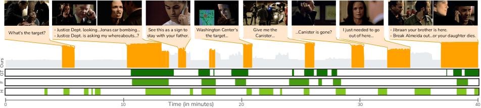
Figure 10: TaleSumm predictions on S07E22 of 24 (test set). “Ours” filled-plot illustrates the importance score profile over time, where orange patches indicate story segments selected for summarization. Annotations are shown below: ground-truth ( GT), fandom ( F) and human annotated ( H). We number the grouped frames representing the predicted contiguous orange chunks as shot groups (SG-n), e.g. this episode has 8 SGs. The story: In a tense sequence, as shown in SG-1, Jack resorts to torture to extract information from Harbinson about the impending attack but is left empty-handed. In SG-2, following the murder of Jonas Hodges, Olivia Taylor faces scrutiny from the Justice Department. Meeting with Martin Collier, she denies transferring funds, revealing a sinister plot. Meanwhile, SG-3 shows Kim Bauer’s plans are disrupted by a flight delay, leading to a strained father-daughter relationship. SG-4,5 displays how Jack, aided by Chloe O’Brian and Renee Walker, captures Tony Almeida and interrogates him about a dangerous canister, followed by Renee uncovering Jibraan’s location, and a high-stakes exchange ensues at the Washington Center station. Jack detonates the canister, succumbing to its effects. As a consequence (SG-6), Cara Bowden reports Tony’s failure to Alan Wilson, adding tension to the unfolding crisis. Olivia returns to the White House, explaining her absence to Aaron Pierce (SG-7), which beautifully connects back to the SG-2. The narrative takes a dire turn as Cara blackmails Jack for the safety of Kim (SG-8), introducing a new layer of suspense and complexity to the unfolding events. The presence of SG-1,6,7 (absent in GT) clearly highlights our model’s ability to complete the overall story arc.

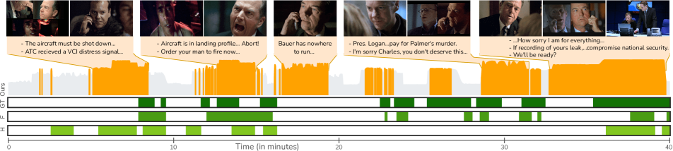
Figure 11: TaleSumm predictions on S05E21 of 24 (test set). “Ours” filled-plot illustrates the importance score profile over time, where orange patches indicate story segments selected for summarization. Annotations are shown below: ground-truth ( GT), fandom ( F), and human annotated ( H). We number the grouped frames representing the predicted contiguous orange chunks as shot groups (SG-n), e.g. this episode has 5 SGs. This episode stands out due to its rapid and significant story advancements, where each sub-story holds apparent importance. Also, human annotations are a bit off in comparison to the ground-truth (can be verified from reliability scores shown in Tab. 10). Importantly, our model considers opinions from all the sources. The story: In the SG-1,2, President Logan, pretending surprised, learns from Admiral Kirkland that Flight 520, now under Jack’s control, is a potential threat. Despite Mike’s doubts about Jack’s intentions, Kirkland urges immediate action, advocating for shooting down the plane. Logan, pretending shock, reluctantly authorizes the attack. Karen alerts Jack to the order, leading to a tense situation. As the plane assumes a landing profile, Kirkland suggests calling off the strike, but Pres. Logan insists on taking it down. Further, in SG-3, Graem criticizes Logan’s decision, emphasizing the importance of capturing Jack, but Logan assures Graem of recapturing him. Meanwhile, in SG-4, Jack, having secured incriminating evidence, vows to make Logan pay for President Palmer’s assassination. In a surprising turn, as shown in SG-5, President Logan contemplates suicide, but an unexpected call from Miles Papazian presents an alternative – the destruction of the recording. Encouraging Miles to act, Logan faces a critical juncture in the unfolding crisis. Overall the entire episode sets the stage for a series of dramatic events, stressing the depth of deceit and the potential consequences for key characters.

B.4 Adapting SoTA Approaches for PlotSnap

In this section, we discuss how we adapt different video- and dialog-only state-of-the-art baselines for our task.

MSVA [20]

considers frame-level features from multiple sources and applies aperture-guided attention across all such feature streams independently, followed by intermediate fusion and a linear classification head that selects frames based on predicted importance scores. Since we are modeling at the level of the entire episode, we feed condensed shot features (after Avg or Max pooling or $\mathsf{ST}$) of each backbone: DenseNet169 ($X_{o}$), MViT ($X_{r}$), and CLIP ($X_{f}$) through three different input streams and output shot-level importance scores.

Our model is different from MSVA as MSVA treats each feature separately, while we perform early fusion and concatenate representations from multiple backbones even before obtaining a compact video shot representation. TaleSumm is also developed for encoding and making predictions on multiple modalities, while MSVA is not.

PGL-SUM [6]

splits the video in small equal-sized group of frames. Similar to our work, contextualization is performed within local multi-headed self-attention on small groups, while another is at global level using global multi-headed attention for the entire video. Later, both are merged via addition along the feature axis and subsequently passed through an MLP classification head to obtain frame-level scores. To adapt PGL-SUM to our work, we again think of shots as the basic unit and concatenate visual features from all streams ($\mathbf{f}^{1},\mathbf{f}^{2}$, and $\mathbf{f}^{3}$), followed by pooling ($\mathsf{ST}$ or Max or Avg pooling) and then PGL-SUM to generate shot-level importance scores.

PGL-SUM has some similarities to our approach as both involve local groups. Interestingly, PGL-SUM creates groups of frames to perform summarization for short videos of a few minutes, while TaleSumm creates groups of shots and dialog utterances to generate summaries for 40 minute long episodes. Among technical contributions, we also explore different attention mechanisms such as across the full-episode (FE) or within a local story group (SG). Different from PGL-SUM, we introduce a story group token that allows to capture the essence of a local story group.

PreSumm [56]

is used for text-only extractive summarization which takes word-level inputs and produces sentence-level probability scores. To represent each episode, the utterances are concatenated, lower-cased, and separated by $\mathsf{CLS}$ and $\mathsf{SEP}$ tokens into a single line input. The PreSumm model leverages word embeddings from pre-trained BERT-base [15] language model. Considering the long inputs in our case, we extend the existing positional embeddings of BERT from 512 to 10000 by keeping the original embeddings and replicating the last embeddings for the remainder. At the sentence level, the corresponding $\mathsf{CLS}$ token is fed into two transformer encoder layers for contextualization, followed by a small MLP and sigmoid operation to generate per-sentence scores. The model is trained using the Adam [45] optimizer with Binary Cross-Entropy loss.

PreSumm is very different from our work as it operates directly on tokens, while our model develops a hierarchical approach going from words to dialogs to local story groups.

A2Summ [28]

is a contemporary multimodal summarization (MSMO) baseline, primarily designed to align temporal correspondence between video and text signals through a dual-contrastive loss approach. They also introduce a dataset, BLiSS [28], comprising 13,303 pairs of livestream videos and transcripts, each with an average duration of 5 minutes, along with multimodal (VT2VT) summaries. A2Summ exploits cross-modality correlations within and between videos through dual contrastive losses. These include: (a) inter-sample contrastive loss (operates across different sample pairs within a batch, leveraging the intrinsic correlations between video-text pairs), and (b) an intra-sample contrastive loss (works within each sample pair, emphasizing the similarities between ground-truth video and text summaries while contrasting positive features with hard-negative features).

We adapt A2Summ for PlotSnap, where we work at the episodic level, by using max-pooling with an MLP for video features and average-pooling for dialog (text) features to derive shot- and utterance-level representations. We create explicit intra-sample attention masks encouraging temporal alignment, allowing video shots to attend to their corresponding utterances and permitting video and utterance tokens to fully attend to their respective counterparts. Considering memory constraints, we maintain a batch size of 4 (four entire episodes - inter-sample contrasting) on a single NVIDIA GeForce RTX-2080 Ti GPU. We adopt CyclicLR [90] with a maximum learning rate of $10^{-4}$ and the ‘triangular2’ mode. A2Summ model comprises 6 encoder layers and incorporates multiple dropout layers [30]: (a) dropout_video ${=}0.1$, (b) dropout_text ${=}0.2$, (c) dropout_attn ${=}0.3$, and (d) dropout_fc ${=}0.5$, while keeping rest the of the hyperparameters the same. Training extends to a maximum of 50 epochs, with the AdamW [58] optimizer utilized, featuring a learning rate of $10^{-5}$ and a weight decay [57] ${=}0.01$.

In PlotSnap, where episodes show related content, the application of inter-episode contrastive learning negatively impacts the model’s performance. This is due to the variability in the importance of related story segments across episodes, which depends on the specific context.

B.5 Details for SumMe and TVSum

	amsgrad	d_model	drop_fc/trm/proj	dec_l	enc_l	wd	act_clf/mlp/trm	ffs
SumMe [24]	True	512	0.5/0.2/0.2	3	1	0.0001	r/g/g	Stack
TVSum [93]	False	768	0.7/0.4/0.2	6	1	0.01	r/g/g	$\boxplus$

Table 13: Hyperparameter configuration for SumMe and TVSum. d_model specify the dimension for the transformer module’s internal representation, while dec_l and enc_l denote $\#$ of decoder and encoder layers, respectively. Other hyperparameters include drop_fc/trm/proj for dropout at classification head, attention module, and projection module, wd stands for weight decay parameter (used inside AdamW [58]), act_clf/mlp/trm for activation function used in classification head, projection, and attention module, with r for ReLU and g for GELU. Lastly, ffs stands for feature fusion style, with Stack and $\boxplus$ depicting the pooling strategy showed in Table 11.

In this section, we will discuss how we adapted our model for SumMe [24] and TVSum [93], some experimentation details, and corresponding evaluation metrics.

Adaptation.

We used our video-based model on both datasets, inheriting features from MSVA [20]. To capture shot-level details, we stacked 15 contiguous frame-embeddings (as previous methods utilized ground-truth labels indexed at every 15th frame), and for group-level, we used n_frame_per_seg attribute of the dataset. We used continuous-index-based time embeddings for shot-frames. Essentially, we assume that a shot consists of 15 frames as SumMe and TVSum require predictions at every 15 frames.

Hyperparameter configuration.

We determine the configuration based on the best validation score obtained over five random splits (5-RCV). This time our model is trained on a single NVIDIA GeForce RTX-2080 Ti GPU for a maximum of 300 epochs for SumMe and 100 epochs for TVSum, with a batch size of 1. Additional dataset-specific hyperparameters are detailed in Table 13. In common, we have AdamW optimizer [58] with parameters: learning rate ${=}5{\times}10^{-5}$, weight decay [57] ${=}10^{-3}$. We use CyclicLR [90] for learning rate scheduling with max lr ${=}5{\times}10^{-4}$ and triangular2 mode. ReLU is used for classification head and GELU for projection and attention modules.

B.6 Extended Qualitative Analysis

In this section, we analyze 3 more episodes and compare the model’s prediction against all three labels (GT, F, and H). Recall, the labels denoted F (Fandom) are based on summarized plot synopses from the 24 fan site that includes the key events in the story (as a text description). Plot synopses are short textual descriptions of the key story events of an episode. We ask annotators to use the plot synopses and tag the start-end duration for story sequences corresponding to the description. We refer to these labels as Fandom (F) and use them for qualitative evaluation. While the H-labels are annotations from a human, based on what they feel is relevant summary as per the narrative.

Qualitative evaluation.

We present importance scores for three episodes: S06E20, S07E22, and S05E21, in Fig. 9, Fig. 10, and Fig. 11, respectively. We observe that the model predictions are quite good and not only match the ground-truth labels (on which the model is trained) but also the fandom and human annotations. Please refer to the figure captions for additional comments on episode-specific remarks.

Appendix C Future Work

Ingesting $\sim$40 minute long videos is a challenging problem. Aligning different modalities, such as processing a 40-minute video containing 2,500 frames (at 1fps) and 4,500 dialogue words, totaling approximately 8000 tokens, may require a larger GPU memory. And most of the L-VLMs [54, 89, 44] struggle to handle contexts exceeding 8,000 tokens, and even if they do, consumer-grade GPUs may lack the capacity to accommodate them.

Our approach considers coarse-grained visual information, which we demonstrate is beneficial for story-summarization. Considering more fine-grained visual info, such as person and face tracks across frames, and their emotions, would be useful. Our idea of using recap-inspired story summary labels or modeling approach are not specific to thrillers and can be easily extended to other genres and shows with recaps. Having speaker information in dialog utterances with mapping to character faces would probably improve performance on the summarization task. The local story groups are a proxy to scene segments of an episode. Replacing them with actual scene segments may improve our model’s performance for summarization.

Finally, further analysis and experiments are required to determine the quality of these methods [97], particularly because evaluating long video summarization using human judgment is very time-consuming.

However, we believe that this work provides a window into this challenging problem and can help facilitate further research in this area.

References

- 24 [2001] 24 (TV series, IMDb). https://www.imdb.com/title/tt0285331/, 2001.
- pb [2005] Prison Break (IMDb). https://www.imdb.com/title/tt0455275/, 2005.
- ccn [2016] Common Crawl - News. https://commoncrawl.org/blog/news-dataset-available, 2016.
- ope [2019] OpenWebText. https://github.com/jcpeterson/openwebtext?tab=readme-ov-file, 2019.
- eng [2021 – Present] English Wikipedia. https://en.wikipedia.org/wiki/English_Wikipedia, 2021 – Present.
- Apostolidis et al. [2021] Evlampios Apostolidis, Georgios Balaouras, Vasileios Mezaris, and Ioannis Patras. Combining Global and Local Attention with Positional Encoding for Video Summarization. In IEEE International Symposium on Multimedia (ISM), 2021.
- Awad et al. [2022] George Awad, Keith Curtis, Asad A. Butt, Jonathan Fiscus, Afzal Godil, Yooyoung Lee, Andrew Delgado, Jesse Zhang, Eliot Godard, Baptiste Chocot, Lukas Diduch, Jeffrey Liu, Yvette Graham, , and Georges Quénot. An overview on the evaluated video retrieval tasks at TRECVID 2022. In Proceedings of TRECVID, 2022.
- Ba et al. [2016] Lei Jimmy Ba, Jamie Ryan Kiros, and Geoffrey E. Hinton. Layer Normalization. arXiv: 1607.06450, 2016.
- Bain et al. [2020] Max Bain, Arsha Nagrani, Andrew Brown, and Andrew Zisserman. Condensed Movies: Story Based Retrieval with Contextual Embeddings, 2020.
- Carreira and Zisserman [2017] João Carreira and Andrew Zisserman. Quo Vadis, Action Recognition? A New Model and the Kinetics Dataset. In Conference on Computer Vision and Pattern Recognition (CVPR), 2017.
- Chen et al. [2022] Mingda Chen, Zewei Chu, Sam Wiseman, and Kevin Gimpel. SummScreen: A Dataset for Abstractive Screenplay Summarization. In Association of Computational Linguistics (ACL), 2022.
- Chen et al. [2023] Shixing Chen, Chun-Hao Liu, Xiang Hao, Xiaohan Nie, Maxim Arap, and Raffay Hamid. Movies2Scenes: Using movie metadata to learn scene representation. In Conference on Computer Vision and Pattern Recognition (CVPR), 2023.
- Chéron et al. [2018] Guilhem Chéron, Jean-Baptiste Alayrac, Ivan Laptev, and Cordelia Schmid. A Flexible Model for Training Action Localization with Varying Levels of Supervision. In Advances in Neural Information Processing Systems (NeurIPS), 2018.
- de Avila et al. [2011] Sandra Eliza Fontes de Avila, Ana Paula Brandão Lopes, Antonio da Luz, and Arnaldo de Albuquerque Araújo. VSUMM: A mechanism designed to produce static video summaries and a novel evaluation method. Pattern Recognition Letters, 32(1):56–68, 2011.
- Devlin et al. [2018] Jacob Devlin, Ming-Wei Chang, Kenton Lee, and Kristina Toutanova. BERT: Pre-training of Deep Bidirectional Transformers for Language Understanding. arXiv:1810.04805, 2018.
- Fan et al. [2021] Haoqi Fan, Bo Xiong, Karttikeya Mangalam, Yanghao Li, Zhicheng Yan, Jitendra Malik, and Christoph Feichtenhofer. Multiscale vision transformers. In International Conference on Computer Vision (ICCV), 2021.
- Fu et al. [2017] Cheng-Yang Fu, Joon Lee, Mohit Bansal, and Alexander Berg. Video Highlight Prediction Using Audience Chat Reactions. In Empirical Methods in Natural Language Processing (EMNLP), 2017.
- Fu et al. [2019] Tsu-Jui Fu, Shao-Heng Tai, and Hwann-Tzong Chen. Attentive and adversarial learning for video summarization. In Winter Conference on Applications of Computer Vision (WACV), 2019.
- Fu et al. [2021] Xiyan Fu, Jun Wang, and Zhenglu Yang. MM-AVS: A Full-Scale Dataset for Multi-modal Summarization. In North American Chapter of Association of Computational Linguistics: Human Language Technologies (NAACL-HLT), 2021.
- Ghauri et al. [2021] Junaid Ahmed Ghauri, Sherzod Hakimov, and Ralph Ewerth. Supervised Video Summarization Via Multiple Feature Sets with Parallel Attention. IEEE International Conference on Multimedia and Expo (ICME), pages 1–6s, 2021.
- Gliwa et al. [2019] Bogdan Gliwa, Iwona Mochol, Maciej Biesek, and Aleksander Wawer. SAMSum Corpus: A Human-annotated Dialogue Dataset for Abstractive Summarization. In Proceedings of the 2nd Workshop on New Frontiers in Summarization, 2019.
- Goldman et al. [2006] Dan B Goldman, Brian Curless, David Salesin, and Steven M. Seitz. Schematic Storyboarding for Video Visualization and Editing. ACM Transactions on Graphics, 25(3):862–871, 2006.
- Gygli et al. [2014a] Michael Gygli, Helmut Grabner, Hayko Riemenschneider, and Luc Van Gool. Creating summaries from user videos. In European Conference on Computer Vision (ECCV). Springer, 2014a.
- Gygli et al. [2014b] Michael Gygli, Helmut Grabner, Hayko Riemenschneider, and Luc Van Gool. Creating summaries from user videos. In European Conference on Computer Vision (ECCV), 2014b.
- Gygli et al. [2015] Michael Gygli, Helmut Grabner, and Luc Van Gool. Video summarization by learning submodular mixtures of objectives. In Conference on Computer Vision and Pattern Recognition (CVPR), 2015.
- Hao et al. [2021] Xiang Hao, Kripa Chettiar, Ben Cheung, Vernon Germano, and Raffay Hamid. Intro and Recap Detection for Movies and TV Series. In Winter Conference on Applications of Computer Vision (WACV), 2021.
- Haurilet et al. [2016] Monica-Laura Haurilet, Makarand Tapaswi, Ziad Al-Halah, and Rainer Stiefelhagen. Naming TV characters by watching and analyzing dialogs. In Winter Conference on Applications of Computer Vision (WACV), 2016.
- He et al. [2023] Bo He, Jun Wang, Jielin Qiu, Trung Bui, Abhinav Shrivastava, and Zhaowen Wang. Align and Attend: Multimodal Summarization with Dual Contrastive Losses. In Conference on Computer Vision and Pattern Recognition (CVPR), 2023.
- He et al. [2015] Kaiming He, X. Zhang, Shaoqing Ren, and Jian Sun. Deep Residual Learning for Image Recognition. In Conference on Computer Vision and Pattern Recognition (CVPR), 2015.
- Hinton et al. [2012] Geoffrey E. Hinton, Nitish Srivastava, Alex Krizhevsky, Ilya Sutskever, and Ruslan Salakhutdinov. Improving neural networks by preventing co-adaptation of feature detectors. ArXiv, abs/1207.0580, 2012.
- Ho et al. [2018] Hsuan-I Ho, Wei-Chen Chiu, and Yu-Chiang Frank Wang. Summarizing First-Person Videos from Third Persons’ Points of Views. In European Conference on Computer Vision (ECCV), 2018.
- Hochreiter and Schmidhuber [1997] Sepp Hochreiter and Jürgen Schmidhuber. Long Short-Term Memory. Neural Computation, 9(8):1735–1780, 1997.
- Houlsby et al. [2019] Neil Houlsby, Andrei Giurgiu, Stanislaw Jastrzebski, Bruna Morrone, Quentin De Laroussilhe, Andrea Gesmundo, Mona Attariyan, and Sylvain Gelly. Parameter-efficient transfer learning for NLP. In International Conference on Machine Learning (ICML), 2019.
- Huang et al. [2017] Gao Huang, Zhuang Liu, Laurens Van Der Maaten, and Kilian Q Weinberger. Densely connected convolutional networks. In Conference on Computer Vision and Pattern Recognition (CVPR), 2017.
- Huang and Worring [2020] Jia-Hong Huang and Marcel Worring. Query-controllable Video Summarization. In International Conference on Multimedia Retrieval (ICMR), 2020.
- Islam et al. [2023] M. Islam, M. Hasan, K. Athrey, T. Braskich, and G. Bertasius. Efficient Movie Scene Detection using State-Space Transformers. In Conference on Computer Vision and Pattern Recognition (CVPR), 2023.
- Islam and Bertasius [2022] Md Mohaiminul Islam and Gedas Bertasius. Long movie clip classification with state-space video models. In European Conference on Computer Vision (ECCV), 2022.
- Jia et al. [2020] Ruipeng Jia, Yanan Cao, Hengzhu Tang, Fang Fang, Cong Cao, and Shi Wang. Neural Extractive Summarization with Hierarchical Attentive Heterogeneous Graph Network. In Empirical Methods in Natural Language Processing (EMNLP), 2020.
- K. et al. [2019] Vivekraj V. K., Debashis Sen, and Balasubramanian Raman. Video Skimming: Taxonomy and Comprehensive Survey. ACM Comput. Surv., 2019.
- Kay et al. [2017] Will Kay, João Carreira, Karen Simonyan, Brian Zhang, Chloe Hillier, Sudheendra Vijayanarasimhan, Fabio Viola, Tim Green, Trevor Back, Apostol Natsev, Mustafa Suleyman, and Andrew Zisserman. The Kinetics Human Action Video Dataset. CoRR, abs/1705.06950, 2017.
- Khan et al. [2022] Zeeshan Khan, C.V. Jawahar, and Makarand Tapaswi. Grounded Video Situation Recognition. In Advances in Neural Information Processing Systems (NeurIPS), 2022.
- Khosla et al. [2013] Aditya Khosla, Raffay Hamid, Chih-Jen Lin, and Neel Sundaresan. Large-Scale Video Summarization Using Web-Image Priors. In Conference on Computer Vision and Pattern Recognition (CVPR), 2013.
- Kim et al. [2014] Gunhee Kim, Leonid Sigal, and Eric P. Xing. Joint Summarization of Large-Scale Collections of Web Images and Videos for Storyline Reconstruction. In Conference on Computer Vision and Pattern Recognition (CVPR), 2014.
- Kim et al. [2021] Wonjae Kim, Bokyung Son, and Ildoo Kim. ViLT: Vision-and-Language Transformer Without Convolution or Region Supervision. In International Conference on Machine Learning, 2021.
- Kingma and Ba [2014] Diederik P. Kingma and Jimmy Ba. Adam: A Method for Stochastic Optimization. arXiv:1412.6980, 2014.
- Kopf et al. [2014] Johannes Kopf, Michael F. Cohen, and Richard Szeliski. First-Person Hyper-Lapse Videos. ACM Transactions on Graphics, 2014.
- Krizhevsky et al. [2009] Alex Krizhevsky, Geoffrey Hinton, et al. Learning multiple layers of features from tiny images. cs.toronto.edu, 2009.
- Kulesza et al. [2012] Alex Kulesza, Ben Taskar, et al. Determinantal point processes for machine learning. Foundations and Trends® in Machine Learning, 5(2–3):123–286, 2012.
- Lee et al. [2012] Yong Jae Lee, Joydeep Ghosh, and Kristen Grauman. Discovering important people and objects for egocentric video summarization. In Conference on Computer Vision and Pattern Recognition (CVPR), 2012.
- Lei et al. [2018] Jie Lei, Licheng Yu, Mohit Bansal, and Tamara Berg. TVQA: Localized, Compositional Video Question Answering. In Empirical Methods in Natural Language Processing (EMNLP), 2018.
- Lei et al. [2020] Jie Lei, Licheng Yu, Tamara Berg, and Mohit Bansal. TVQA+: Spatio-Temporal Grounding for Video Question Answering. In Association of Computational Linguistics (ACL), 2020.
- Levesque et al. [2012] Hector J. Levesque, Ernest Davis, and Leora Morgenstern. The winograd schema challenge. In Proceedings of the Thirteenth International Conference on Principles of Knowledge Representation and Reasoning, 2012.
- Lewis et al. [2020] Mike Lewis, Yinhan Liu, Naman Goyal, Marjan Ghazvininejad, Abdelrahman Mohamed, Omer Levy, Veselin Stoyanov, and Luke Zettlemoyer. BART: Denoising sequence-to-sequence pre-training for natural language generation, translation, and comprehension. In Association of Computational Linguistics (ACL), 2020.
- Li et al. [2022] Junnan Li, Dongxu Li, Caiming Xiong, and Steven C. H. Hoi. BLIP: Bootstrapping Language-Image Pre-training for Unified Vision-Language Understanding and Generation. In International Conference on Machine Learning, 2022.
- Lin et al. [2023] Jingyang Lin, Hang Hua, Ming Chen, Yikang Li, Jenhao Hsiao, Chiuman Ho, and Jiebo Luo. VideoXum: Cross-modal Visual and Textural Summarization of Videos. IEEE Transactions on Multimedia, 2023.
- Liu and Lapata [2019] Yang Liu and Mirella Lapata. Text Summarization with Pretrained Encoders. In Empirical Methods in Natural Language Processing and the 9th International Joint Conference on Natural Language Processing (EMNLP-IJCNLP), 2019.
- Loshchilov and Hutter [2017a] Ilya Loshchilov and Frank Hutter. Decoupled Weight Decay Regularization. In International Conference on Learning Representations (ICLR), 2017a.
- Loshchilov and Hutter [2017b] Ilya Loshchilov and Frank Hutter. Decoupled Weight Decay Regularization. In International Conference on Learning Representations (ICLR), 2017b.
- Lu and Grauman [2013] Zheng Lu and Kristen Grauman. Story-Driven Summarization for Egocentric Video. In Conference on Computer Vision and Pattern Recognition (CVPR), 2013.
- Ma et al. [2021] Mingyang Ma, Shaohui Mei, Shuai Wan, Zhiyong Wang, David Dagan Feng, and Mohammed Bennamoun. Similarity Based Block Sparse Subset Selection for Video Summarization. IEEE Transactions on Circuits and Systems for Video Technology, 31(10):3967–3980, 2021.
- Nagrani and Zisserman [2017] Arsha Nagrani and Andrew Zisserman. From Benedict Cumberbatch to Sherlock Holmes: Character Identification in TV series without a Script. In British Machine Vision Conference (BMVC), 2017.
- Nagrani et al. [2018] Arsha Nagrani, Samuel Albanie, and Andrew Zisserman. Learnable PINs: Cross-Modal Embeddings for Person Identity. In European Conference on Computer Vision (ECCV), 2018.
- Nallapati et al. [2016a] Ramesh Nallapati, Bowen Zhou, Cicero dos Santos, Çaglar Gulçehre, and Bing Xian. Abstractive Text Summarization using Sequence-to-sequence RNNs and Beyond. In Computational Natural Language Learning (CoNLL), 2016a.
- Nallapati et al. [2016b] Ramesh Nallapati, Bowen Zhou, Caglar Gulcehre, and Bing Xiang. Abstractive Text Summarization using Sequence-to-sequence RNNs and Beyond. In Computational Natural Language Learning (CoNLL), 2016b.
- Narasimhan et al. [2021] Medhini Narasimhan, Anna Rohrbach, and Trevor Darrell. Clip-It! Language-guided Video Summarization. In Advances in Neural Information Processing Systems (NeurIPS), 2021.
- Narayan et al. [2018] Shashi Narayan, Shay B. Cohen, and Mirella Lapata. Don’t Give Me the Details, Just the Summary! Topic-Aware Convolutional Neural Networks for Extreme Summarization. In Empirical Methods in Natural Language Processing (EMNLP), 2018.
- Otani et al. [2019] Mayu Otani, Yuta Nakashima, Esa Rahtu, and Janne Heikkilä. Rethinking the Evaluation of Video Summaries. In Conference on Computer Vision and Pattern Recognition (CVPR), 2019.
- Papalampidi and Lapata [2022] Pinelopi Papalampidi and Mirella Lapata. Hierarchical3D Adapters for Long Video-to-text Summarization. arXiv:2210.04829, 2022.
- Papalampidi et al. [2019] Pinelopi Papalampidi, Frank Keller, and Mirella Lapata. Movie Plot Analysis via Turning Point Identification. In Empirical Methods in Natural Language Processing and the 9th International Joint Conference on Natural Language Processing (EMNLP-IJCNLP), 2019.
- Papalampidi et al. [2020] Pinelopi Papalampidi, Frank Keller, Lea Frermann, and Mirella Lapata. Screenplay Summarization Using Latent Narrative Structure. In Association of Computational Linguistics (ACL), 2020.
- Papalampidi et al. [2021a] Pinelopi Papalampidi, Frank Keller, and Mirella Lapata. Film trailer generation via task decomposition. arXiv preprint arXiv:2111.08774, 2021a.
- Papalampidi et al. [2021b] Pinelopi Papalampidi, Frank Keller, and Mirella Lapata. Movie Summarization via Sparse Graph Construction. In Association for the Advancement of Artificial Intelligence (AAAI), 2021b.
- Park et al. [2020] Jae Sung Park, Trevor Darrell, and Anna Rohrbach. Identity-Aware Multi-Sentence Video Description. In European Conference on Computer Vision (ECCV), 2020.
- Paszke et al. [2019] Adam Paszke, Sam Gross, Francisco Massa, Adam Lerer, James Bradbury, Gregory Chanan, Trevor Killeen, Zeming Lin, Natalia Gimelshein, Luca Antiga, Alban Desmaison, Andreas Kopf, Edward Yang, Zachary DeVito, Martin Raison, Alykhan Tejani, Sasank Chilamkurthy, Benoit Steiner, Lu Fang, Junjie Bai, and Soumith Chintala. PyTorch: An Imperative Style, High-Performance Deep Learning Library. In Advances in Neural Information Processing Systems (NeurIPS), 2019.
- Pini et al. [2019] Stefano Pini, Marcella Cornia, Federico Bolelli, Lorenzo Baraldi, and Rita Cucchiara. M-VAD Names: A Dataset for Video Captioning with Naming. Multimedia Tools Appl., page 14007–14027, 2019.
- Pritch et al. [2008] Yael Pritch, Alex Rav-Acha, and Shmuel Peleg. Nonchronological Video Synopsis and Indexing. In IEEE Transactions on Pattern Analysis and Machine Intelligence (PAMI), 2008.
- Radford et al. [2019] Alec Radford, Jeffrey Wu, Rewon Child, David Luan, Dario Amodei, Ilya Sutskever, et al. Language models are unsupervised multitask learners. OpenAI blog, 1(8):9, 2019.
- Radford et al. [2021] Alec Radford, Jong Wook Kim, Chris Hallacy, Aditya Ramesh, Gabriel Goh, Sandhini Agarwal, Girish Sastry, Amanda Askell, Pamela Mishkin, Jack Clark, et al. Learning transferable visual models from natural language supervision. In International Conference on Machine Learning (ICML). PMLR, 2021.
- Raffel et al. [2020] Colin Raffel, Noam Shazeer, Adam Roberts, Katherine Lee, Sharan Narang, Michael Matena, Yanqi Zhou, Wei Li, and Peter J Liu. Exploring the limits of transfer learning with a unified text-to-text transformer. Journal of Machine Learning Research (JMLR), 2020.
- Rochan and Wang [2019] Mrigank Rochan and Yang Wang. Video summarization by learning from unpaired data. In Conference on Computer Vision and Pattern Recognition (CVPR), 2019.
- Rohrbach et al. [2014] Anna Rohrbach, Marcus Rohrbach, Weijian Qiu, Annemarie Friedrich, Manfred Pinkal, and Bernt Schiele. Coherent Multi-sentence Video Description with Variable Level of Detail. In German Conference on Pattern Recognition (GCPR), 2014.
- Rohrbach et al. [2015] Anna Rohrbach, Marcus Rohrbach, Niket Tandon, and Bernt Schiele. A dataset for Movie Description. In Conference on Computer Vision and Pattern Recognition (CVPR), 2015.
- Rohrbach et al. [2017] Anna Rohrbach, Atousa Torabi, Marcus Rohrbach, Niket Tandon, Christopher Pal, Hugo Larochelle, Aaron Courville, and Bernt Schiele. Movie Description. International Journal of Computer Vision (IJCV), 123(1):94–120, 2017.
- Russakovsky et al. [2015] Olga Russakovsky, Jia Deng, Hao Su, Jonathan Krause, Sanjeev Satheesh, Sean Ma, Zhiheng Huang, Andrej Karpathy, Aditya Khosla, Michael Bernstein, Alexander C. Berg, and Li Fei-Fei. ImageNet Large Scale Visual Recognition Challenge. International Journal of Computer Vision (IJCV), pages 211–252, 2015.
- Sadhu et al. [2021] Arka Sadhu, Tanmay Gupta, Mark Yatskar, Ram Nevatia, and Aniruddha Kembhavi. Visual Semantic Role Labeling for Video Understanding. In Conference on Computer Vision and Pattern Recognition (CVPR), 2021.
- Sanabria et al. [2018] Ramon Sanabria, Ozan Caglayan, Shruti Palaskar, Desmond Elliott, Loïc Barrault, Lucia Specia, and Florian Metze. How2: A Large-scale Dataset for Multimodal Language Understanding. In Advances in Neural Information Processing Systems-Workshop (NeurIPS-W), 2018.
- Sankar et al. [2009] K. Pramod Sankar, C. V. Jawahar, and Andrew Zisserman. Subtitle-free Movie to Script Alignment. In British Machine Vision Conference (BMVC), 2009.
- Saquil et al. [2021] Yassir Saquil, Da Chen, Yuan He, Chuan Li, and Yong-Liang Yang. Multiple Pairwise Ranking Networks for Personalized Video Summarization. In International Conference on Computer Vision (ICCV), 2021.
- Singh et al. [2022] Amanpreet Singh, Ronghang Hu, Vedanuj Goswami, Guillaume Couairon, Wojciech Galuba, Marcus Rohrbach, and Douwe Kiela. FLAVA: A foundational language and vision alignment model. In CVPR, 2022.
- Smith [2015] Leslie N. Smith. Cyclical Learning Rates for Training Neural Networks. In Winter Conference on Applications of Computer Vision (WACV), 2015.
- Smith and Topin [2018] Leslie N. Smith and Nicholay Topin. Super-convergence: very fast training of neural networks using large learning rates. In Defense + Commercial Sensing, 2018.
- Song et al. [2020] Kaitao Song, Xu Tan, Tao Qin, Jianfeng Lu, and Tie-Yan Liu. MPNet: Masked and Permuted Pre-Training for Language Understanding. In Advances in Neural Information Processing Systems (NeurIPS), 2020.
- Song et al. [2015] Yale Song, Jordi Vallmitjana, Amanda Stent, and Alejandro Jaimes. TVSum: Summarizing web videos using titles. In Conference on Computer Vision and Pattern Recognition (CVPR), 2015.
- Srivastava et al. [2023] Dhruv Srivastava, Aditya Kumar Singh, and Makarand Tapaswi. How you feelin’? Learning Emotions and Mental States in Movie Scenes. In Conference on Computer Vision and Pattern Recognition (CVPR), 2023.
- Sun et al. [2014] Min Sun, Ali Farhadi, Ben Taskar, and Steve Seitz. Salient montages from unconstrained videos. In European Conference on Computer Vision (ECCV), 2014.
- Szegedy et al. [2015] Christian Szegedy, Wei Liu, Yangqing Jia, Pierre Sermanet, Scott Reed, Dragomir Anguelov, Dumitru Erhan, Vincent Vanhoucke, and Andrew Rabinovich. Going deeper with convolutions. In Conference on Computer Vision and Pattern Recognition (CVPR), 2015.
- Tang et al. [2023] Liyan Tang, Tanya Goyal, Alex Fabbri, Philippe Laban, Jiacheng Xu, Semih Yavuz, Wojciech Kryscinski, Justin Rousseau, and Greg Durrett. Understanding Factual Errors in Summarization: Errors, Summarizers, Datasets, Error Detectors. In Association of Computational Linguistics (ACL), 2023.
- Tapaswi et al. [2014a] Makarand Tapaswi, Martin Bäuml, and Rainer Stiefelhagen. Story-Based Video Retrieval in TV Series Using Plot Synopses. In International Conference on Multimedia Retrieval (ICMR), 2014a.
- Tapaswi et al. [2014b] Makarand Tapaswi, Martin Bäuml, and Rainer Stiefelhagen. StoryGraphs: Visualizing Character Interactions as a Timeline. In Conference on Computer Vision and Pattern Recognition (CVPR), 2014b.
- Tapaswi et al. [2015] Makarand Tapaswi, Martin Bäuml, and Rainer Stiefelhagen. Aligning plot synopses to videos for story-based retrieval. International Journal of Multimedia Information Retrieval (IJMIR), 4(1):3–16, 2015.
- Tapaswi et al. [2016] Makarand Tapaswi, Yukun Zhu, Rainer Stiefelhagen, Antonio Torralba, Raquel Urtasun, and Sanja Fidler. MovieQA: Understanding Stories in Movies through Question-Answering. In Conference on Computer Vision and Pattern Recognition (CVPR), 2016.
- Tengda Han and Max Bain and Arsha Nagrani and Gül Varol and Weidi Xie and Andrew Zisserman [2023] Tengda Han and Max Bain and Arsha Nagrani and Gül Varol and Weidi Xie and Andrew Zisserman. AutoAD II: The Sequel - Who, When, and What in Movie Audio Description. In International Conference on Computer Vision (ICCV), 2023.
- Trinh and Le [2018] Trieu H. Trinh and Quoc V. Le. A Simple Method for Commonsense Reasoning. ArXiv, abs/1806.02847, 2018.
- Vaswani et al. [2017] Ashish Vaswani, Noam Shazeer, Niki Parmar, Jakob Uszkoreit, Llion Jones, Aidan N Gomez, Ł ukasz Kaiser, and Illia Polosukhin. Attention is All you Need. In Advances in Neural Information Processing Systems (NeurIPS), 2017.
- Vicol et al. [2018] Paul Vicol, Makarand Tapaswi, Lluis Castrejon, and Sanja Fidler. MovieGraphs: Towards Understanding Human-Centric Situations from Videos. In Conference on Computer Vision and Pattern Recognition (CVPR), 2018.
- Wolf et al. [2019] Thomas Wolf, Lysandre Debut, Victor Sanh, Julien Chaumond, Clement Delangue, Anthony Moi, Pierric Cistac, Tim Rault, Rémi Louf, Morgan Funtowicz, et al. Huggingface’s transformers: State-of-the-art natural language processing. arXiv preprint arXiv:1910.03771, 2019.
- Wolf [1996] W. Wolf. Key Frame Selection by Motion Analysis. In International Conference on Acoustics, Speech and Signal Processing (ICASSP), 1996.
- Xiao et al. [2022] F. Xiao, K. Kundu, J. Tighe, and D. Modolo. Hierarchical Self-supervised Representation Learning for Movie Understanding. In Conference on Computer Vision and Pattern Recognition (CVPR), 2022.
- Yusoff et al. [1998] Yusseri Yusoff, William J. Christmas, and Josef Kittler. A Study on Automatic Shot Change Detection. In European Conference on Multimedia Applications, Services and Techniques, 1998.
- Yuval [2011] Netzer Yuval. Reading digits in Natural Images with Unsupervised Feature Learning. In Advances in Neural Information Processing Systems-Workshop (NeurIPS-W), 2011.
- Zeng et al. [2016] Kuo-Hao Zeng, Tseng-Hung Chen, Juan Carlos Niebles, and Min Sun. Title Generation for User Generated Videos. In European Conference on Computer Vision (ECCV), 2016.
- Zhang et al. [2020] Jingqing Zhang, Yao Zhao, Mohammad Saleh, and Peter Liu. Pegasus: Pre-training with extracted gap-sentences for abstractive summarization. In International Conference on Machine Learning (ICML). PMLR, 2020.
- Zhang et al. [2016a] Ke Zhang, Wei-Lun Chao, Fei Sha, and Kristen Grauman. Summary Transfer: Exemplar-based Subset Selection for Video Summarization. CoRR, abs/1603.03369, 2016a.
- Zhang et al. [2016b] Ke Zhang, Wei-Lun Chao, Fei Sha, and Kristen Grauman. Video summarization with long short-term memory. In European Conference on Computer Vision (ECCV), 2016b.
- Zhang et al. [2018] Ke Zhang, Kristen Grauman, and Fei Sha. Retrospective encoders for video summarization. In European Conference on Computer Vision (ECCV), 2018.
- Zhang et al. [2019] Yujia Zhang, Michael Kampffmeyer, Xiaoguang Zhao, and Min Tan. DTR-GAN: Dilated temporal relational adversarial network for video summarization. In Proceedings of the ACM Turing Celebration Conference-China, 2019.
- Zhong et al. [2020] Ming Zhong, Pengfei Liu, Yiran Chen, Danqing Wang, Xipeng Qiu, and Xuanjing Huang. Extractive Summarization as Text Matching. In Association of Computational Linguistics (ACL), 2020.
- Zhu et al. [2018] Junnan Zhu, Haoran Li, Tianshang Liu, Yu Zhou, Jiajun Zhang, and Chengqing Zong. MSMO: Multimodal Summarization with Multimodal Output. In Empirical Methods in Natural Language Processing (EMNLP), 2018.
- Zhu et al. [2021] Wencheng Zhu, Jiwen Lu, Jiahao Li, and Jie Zhou. DSNet: A Flexible Detect-to-Summarize Network for Video Summarization. IEEE Transactions on Image Processing, 30:948–962, 2021.
- Zhu et al. [2022] Wencheng Zhu, Yucheng Han, Jiwen Lu, and Jie Zhou. Relational reasoning over spatial-temporal graphs for video summarization. IEEE Transactions on Image Processing, 31:3017–3031, 2022.
- Zhu et al. [2015a] Yukun Zhu, Ryan Kiros, Richard Zemel, Ruslan Salakhutdinov, Raquel Urtasun, Antonio Torralba, and Sanja Fidler. Aligning Books and Movies: Towards Story-like Visual Explanations by Watching Movies and Reading Books. In arXiv preprint arXiv:1506.06724, 2015a.
- Zhu et al. [2015b] Yukun Zhu, Ryan Kiros, Richard S. Zemel, Ruslan Salakhutdinov, Raquel Urtasun, Antonio Torralba, and Sanja Fidler. Aligning Books and Movies: Towards Story-Like Visual Explanations by Watching Movies and Reading Books. In International Conference on Computer Vision (ICCV), 2015b.
- Zhuang et al. [2021] Liu Zhuang, Lin Wayne, Shi Ya, and Zhao Jun. A Robustly Optimized BERT Pre-training Approach with Post-training. In Proceedings of the 20th Chinese National Conference on Computational Linguistics, 2021.