Normal traces and applications
to continuity equations on bounded domains

Abstract.

In this work, we study several properties of the normal Lebesgue trace of vector fields introduced by the second and third author in [DRINV23] in the context of the energy conservation for the Euler equations in Onsager-critical classes. Among several properties, we prove that the normal Lebesgue trace satisfies the Gauss-Green identity and, by providing explicit counterexamples, that it is a notion sitting strictly between the distributional one for measure-divergence vector fields and the strong one for $BV$ functions. These results are then applied to the study of the uniqueness of weak solutions for continuity equations on bounded domains, allowing to remove the assumption in [CDS14] of global $BV$ regularity up to the boundary, at least around the portion of the boundary where the characteristics exit the domain or are tangent. The proof relies on an explicit renormalization formula completely characterized by the boundary datum and the positive part of the normal Lebesgue trace. In the case when the characteristics enter the domain, a counterexample shows that achieving the normal trace in the Lebesgue sense is not enough to prevent non-uniqueness, and thus a $BV$ assumption seems to be necessary for the uniqueness of weak solutions.

1. Introduction

Throughout this note we will work in any spatial dimension $d\geq 2$. Before stating our main results, we start by recalling some definitions and explaining the main context.

Definition 1.1 ($L^{p}$ Measure-divergence vector fields).

Let $1\leq p\leq\infty$ and let $\Omega\subset\mathbb{R}^{d}$ be an open set. Given a vector field $u:\Omega\rightarrow\mathbb{R}^{d}$ we say that $u\in\mathcal{MD}^{p}(\Omega)$ if $u\in L^{p}(\Omega)$ and $\mathop{\rm div}\nolimits u\in\mathcal{M}(\Omega)$.

Here $\mathcal{M}(\Omega)$ denotes the space of finite measures over the open set $\Omega$. Building on an intuition by Anzellotti [Anz83, Anz83bis], a weak (distributional) notion of normal trace can be defined by imposing the validity of the Gauss-Green identity.

Definition 1.2 (Distributional normal trace).

Let $\Omega\subset\mathbb{R}^{d}$ be a bounded open set with Lipschitz boundary. Given a vector field $u\in\mathcal{MD}^{1}(\Omega)$, and denoting $\lambda=\mathop{\rm div}\nolimits u$, we define its outward distributional normal trace on $\partial\Omega$ by

$$\langle\mathop{\rm Tr}\nolimits_{n}(u;\partial\Omega),\varphi\rangle:=\int_{\Omega}\varphi\,d\lambda+\int_{\Omega}u\cdot\nabla\varphi\,dy\qquad\forall\varphi\in C^{\infty}_{c}(\mathbb{R}^{d}).$$ (1.1)

Note that by a standard density argument, considering $\varphi\in\mathop{\rm Lip}\nolimits_{c}(\mathbb{R}^{d})$ in (1.1) yields an equivalent definition. Clearly $\mathop{\rm Tr}\nolimits_{n}(u;\partial\Omega)$ is in general a distribution of order $1$. However, see for instance [ACM05]*Proposition 3.2, in the case $u\in\mathcal{MD}^{\infty}(\Omega)$ the distributional trace is in fact induced by a measurable function and $\mathop{\rm Tr}\nolimits_{n}(u;\partial\Omega)\in L^{\infty}(\partial\Omega;\mathcal{H}^{d-1})$. Note also that we are adopting the convention that $n:\partial\Omega\rightarrow\mathbb{S}^{d-1}$ is the outward unit normal vector, which will be kept through the whole manuscript.

Measure-divergence vector fields, with particular emphasis on the case $p=\infty$, have received great attention in recent years. They happen to be very useful in several contexts such as establishing fine properties of vector fields with bounded deformation [ACM05], existence and uniqueness for continuity-type equations with a physical boundary [CDS14, CDS14bis], conservation laws [CTZ09, CT11, CTZ07, CT05, CF99], dissipative anomalies and intermittency in turbulent flows [DDI23] and several others. For a detailed analysis of the theoretical properties and refinements of $\mathcal{MD}^{p}$ we refer the interested reader to [PT08, CCT19, Sil23, Sil05] and references therein.

1.1. The normal Lebesgue trace

The downside of the generality of Definition 1.2 is in that it does not prevent bad behaviours of the vector field $u$ in the proximity of $\partial\Omega$. For instance in [CDS14] it has been shown that having a distributional trace of the vector field is not enough to guarantee uniqueness for transport and/or continuity equations on a domain $\Omega$ with boundary, even when a boundary datum is properly assigned. On the positive side, in the same paper [CDS14] it has been also shown that a $BV$ assumption on $u$ up to the boundary does imply uniqueness, the main reason being the fact that $BV$ functions achieve their traces in a sufficiently strong sense (see Section 2 for the definition and main properties of $BV$ functions). More recently, a new notion of normal Lebesgue boundary trace has been introduced in [DRINV23] in the context of the energy conservation for the Euler equations in Onsager-critical classes. We recall here this notion.

Definition 1.3 (Normal Lebesgue boundary trace).

Let $\Omega\subset\mathbb{R}^{d}$ be a bounded open set with Lipschitz boundary and let $u\in L^{1}(\Omega)$ be a vector field. We say that $u$ admits an inward Lebesgue normal trace on $\partial\Omega$ if there exists a function $f\in L^{1}(\partial\Omega;\mathcal{H}^{d-1})$ such that, for every sequence $r_{k}\rightarrow 0$, it holds

$$\lim_{k\to\infty}\frac{1}{r_{k}^{d}}\int_{B_{r_{k}}(x)\cap\Omega}\left|(u\cdot\nabla d_{\partial\Omega})(y)-f(x)\right|\,dy=0\qquad\text{for }\mathcal{H}^{d-1}\text{-a.e. }x\in\partial\Omega.$$

Whenever such a function exists, we will denote it by $f=:u_{-n}^{\partial\Omega}$. Consequently, the outward Lebesgue normal trace will be $u_{n}^{\partial\Omega}:=-u_{-n}^{\partial\Omega}$.

It is an easy check that, whenever it exists, the normal Lebesgue trace is unique (see [DRINV23]*Section 5.1). Note that here, to keep consistency with $\mathop{\rm Tr}\nolimits_{n}(u;\partial\Omega)$ being the outward normal distributional trace, we are adopting the opposite convention with respect to [DRINV23]*Definition 5.2 by switching the sign. The above definition has been used in the context of weak solutions to the incompressible Euler equations to prevent the energy dissipation from happening at the boundary [DRINV23]*Theorem 1.3. It has also been proved (see the proof of [DRINV23]*Proposition 5.5) that for $u\in BV$ the normal Lebesgue boundary trace exists, with explicit representation with respect to the full trace of the vector field. Clearly, the definition of the normal Lebesgue trace can be restricted to any measurable subset $\Sigma\subset\partial\Omega$. This will be done in Section 3.2, together with the study of further properties which will be important for the application to the continuity equations on bounded domains. Due to the very weak regularity of the objects involved, our analysis requires several technical tools from geometric measure theory and in particular establishes properties of sets with Lipschitz boundary that might be interesting in themselves.

From now on we restrict ourselves to bounded vector fields, since otherwise the distributional normal trace might fail to be induced by a function. Our first main result shows that, for $u\in\mathcal{MD}^{\infty}$, if the normal Lebesgue trace exists it must coincide with the distributional one. In particular, it satisfies the Gauss-Green identity.

Theorem 1.4.

Let $\Omega\subset\mathbb{R}^{d}$ be a bounded open set with Lipschitz boundary and let $u\in\mathcal{MD}^{\infty}(\Omega)$. Assume that $u$ has a normal Lebesgue trace on $\partial\Omega$ in the sense of Definition 1.3. Then, it holds $u_{n}^{\partial\Omega}\equiv\mathop{\rm Tr}\nolimits_{n}(u;\partial\Omega)$ as elements of $L^{\infty}(\partial\Omega;\mathcal{H}^{d-1})$.

In particular, for bounded measure-divergence vector fields, either the normal Lebesgue trace does not exist or it exists and it coincides with the distributional one. This observation will be used in Lemma 3.11 to construct $u\in\mathcal{MD}^{\infty}$ which does not admit a normal Lebesgue trace. Moreover it is rather easy to find vector fields which do admit a normal Lebesgue trace but fail to be of bounded variation (see Remark 2.5). It follows that Definition 1.3 is a notion lying strictly between the distributional one of Definition 1.2 and the strong one for $BV$ vector fields (see Theorem 2.4). In Section 3 we also prove some additional properties of the normal Lebesgue trace which might be of independent interest. Let us point out that here all the results assume the vector field to be bounded. Since Definition 1.2 and Definition 1.3 make sense for $L^{1}$ vector fields, the following question is motivated.

Question 1.5.

Let $\Omega\subset\mathbb{R}^{d}$ be a bounded open set with Lipschitz boundary and let $u\in\mathcal{MD}^{1}(\Omega)$. Assume that $u$ has an outward normal Lebesgue trace on $\partial\Omega$ in the sense of Definition 1.3. Is it true that $\mathop{\rm Tr}\nolimits_{n}(u;\partial\Omega)\in L^{1}(\partial\Omega;\mathcal{H}^{d-1})$ and $u_{n}^{\partial\Omega}=\mathop{\rm Tr}\nolimits_{n}(u;\partial\Omega)$ as elements of $L^{1}(\partial\Omega;\mathcal{H}^{d-1})$?

1.2. Applications to the continuity equation

The groundbreaking theory of renormalized solutions by DiPerna–Lions [DipLi89] and Ambrosio [Ambr04] establishes the well-posedness for weak solutions of the continuity equation with rough vector fields on the whole space $\mathbb{R}^{d}$, more precisely, in the case of Sobolev and $BV$ vector fields respectively. See for instance [CripDel08, Cr09] for a review.

Let us now focus on the bounded domain setting. Since we will be working with merely bounded solutions, the rigorous definitions become quite delicate. For this reason we postpone to Section 4 the main technical formulations which guarantee that all the objects involved are well defined. We consider a solution $\rho:\Omega\times(0,T)\rightarrow\mathbb{R}$ to

$$\left\{\begin{array}[]{rcll}\partial_{t}\rho+\mathop{\rm div}\nolimits(\rho u)&=&c\rho+f&\text{ in }\Omega\times(0,T)\\ \rho&=&g&\text{ on }\Gamma^{-}\\ \rho(\cdot,0)&=&\rho_{0}&\text{ in }\Omega,\end{array}\right.$$ (1.2)

where $\Omega\subset\mathbb{R}^{d}$ is an open bounded set with Lipschitz boundary, $u:\Omega\times(0,T)\rightarrow\mathbb{R}^{d}$ is a given vector field, $\Gamma^{-}\subset\partial\Omega\times(0,T)$ is the (possibly time-dependent) portion of the boundary in which the characteristics are entering, while $\rho_{0}:\Omega\rightarrow\mathbb{R}$, $g:\Gamma^{-}\rightarrow\mathbb{R}$ and $c,f:\Omega\times(0,T)\rightarrow\mathbb{R}$ are given data. Note that if $\rho$ and $u$ are not sufficiently regular their value on negligible sets is not well defined. However, as noted in [CDS14bis], a distributional formulation of the problem (1.2) can still be given by relying on the theory of measure-divergence vector fields described above, see Definition 4.3. The existence of such weak solutions has been proved in [CDS14bis] by parabolic regularization under quite general assumptions. A much more delicate issue is the uniqueness of weak solutions, which has been established in [CDS14] under the assumption that $u\in L^{1}_{\rm loc}([0,T);BV(\Omega))$, that is when the vector field enjoys $BV$ regularity up to the boundary. The uniqueness result heavily relies on a suitable chain-rule formula for the normal trace of $\rho^{2}u$ at the boundary, previously established in [ACM05]*Theorem 4.2, which holds when $u\in BV(\Omega)$. Our main goal is to show that no $BV$ assumption on $u$ is necessary around the portion of the boundary where the characteristics exit, as soon as a suitable behaviour in terms of the normal Lebesgue trace is assumed.

In the next theorem, for a set $A\subset\partial\Omega$, we will denote its $r$-tubular neighbourhood “interior to $\Omega$” by $(A)_{r}^{\rm in}:=(A)_{r}\cap\Omega$, where $(A)_{r}$ is the standard tubular neighbourhood (in $\mathbb{R}^{d}$) of width $r>0$. We refer to Section 2.1 for a more detailed guideline on the notation used in this whole note.

Theorem 1.6.

Let $\Omega\subset\mathbb{R}^{d}$ be a bounded open set with Lipschitz boundary and $u\in L^{\infty}(\Omega\times(0,T))\cap L^{1}_{\rm loc}([0,T);BV_{\rm loc}(\Omega))$ be a vector field such that $\mathop{\rm div}\nolimits u\in L^{1}((0,T);L^{\infty}(\Omega))$. Let $\Gamma^{-},\Gamma^{+}\subset\partial\Omega\times(0,T)$ be as in Definition 4.1 and assume that

• there exists an open set $O\subset\mathbb{R}^{d}\times(0,T)$ such that $\Gamma^{-}\subset O$, $u_{t}\in BV_{\rm loc}(O_{t})$ for a.e. $t\in(0,T)$ and $\nabla u_{t}\otimes dt\in\mathcal{M}_{\rm loc}(O)$,

• denoting by $\Gamma^{+}_{t}\subset\partial\Omega$ the $t$-time slice of the space-time set $\Gamma^{+}$, for a.e. $t\in(0,T)$ it holds

  $$\lim_{r\rightarrow 0}\frac{1}{r}\int_{(\Gamma^{+}_{t})_{r}^{\rm in}}(u_{t}\cdot\nabla d_{\partial\Omega})_{+}\,dx=0.$$ (1.3)

Moreover, let $f\in L^{1}(\Omega\times(0,T))$, $c\in L^{1}((0,T);L^{\infty}(\Omega))$, $\rho_{0}\in L^{\infty}(\Omega)$ and $g\in L^{\infty}(\Gamma^{-})$ be given. Then, in the class $\rho\in L^{\infty}(\Omega\times(0,T))$, the problem (1.2) admits at most one distributional solution in the sense of Definition 4.3.

Remark 1.7 (Existence).

Theorem 1.6 is concerned only with uniqueness. The existence part, in the case $\mathop{\rm div}\nolimits u,f,c\in L^{\infty}(\Omega\times(0,T))$ is more classical and can be found in [CDS14bis]. Notice that the generalization to the case $f\in L^{1}(\Omega\times(0,T))$, $c\in L^{1}((0,T);L^{\infty}(\Omega))$ directly follows by a standard truncation argument together with the a priori bound on the solution.

A more general version of the above theorem will be given in Section 4 (see Theorem 4.5 and Corollary 4.6) where we prove that an explicit weak formulation for $\beta(\rho)$ holds up to the boundary, for any $\beta\in C^{1}(\mathbb{R})$, that is the vector field $u$ satisfies a renormalization property on $\Omega\times[0,T)$. The renormalization property can be seen in a certain sense as an analogue in the linear case of the conservation of the energy studied in [DRINV23] in the context of the Euler equations. In particular, it is natural to investigate the role of the normal Lebesgue trace for the renormalization property. The assumption (1.3) can be thought of as a way to force characteristics to be “uniformly” exiting, which we will show to be enough to prevent non-uniqueness phenomena. Equivalently, (1.3) dampens any “recoil” of the vector field which could cause mass to enter the domain $\Omega$ around the portion of $\partial\Omega$ where on average (i.e. in the weak sense) it points outward, a phenomenon which relates to ill-posedness. More effective conditions in terms of the normal Lebesgue trace from Definition 1.3 which imply (1.3) will be given in Section 3.2 (see for instance Corollary 3.9). As a consequence of our general results on the relation between the normal Lebesgue trace and the distributional one, in Proposition 3.10 we will show that (1.3) holds true as soon as $u$ is $BV$ up to the boundary, while in general it is a strictly weaker assumption. In some sense, Theorem 1.6 shows that the subset of the boundary in which characteristics are entering, i.e. $\Gamma^{-}$, is more problematic than $\Gamma^{+}$ since it requires the vector field to be $BV$ in its neighbourhood. Indeed, we notice that in the counter-example built in [CDS14] the vector field achieves the normal boundary trace in the strong Lebesgue sense.

Proposition 1.8.

Let $\Omega:=\mathbb{R}^{2}\times(0,+\infty)$. There exists an autonomous vector field $u:\Omega\rightarrow\mathbb{R}^{3}$ such that $\mathop{\rm div}\nolimits u=0$, $u\in L^{\infty}(\Omega)\cap BV_{\rm loc}(\Omega)$, $\mathop{\rm Tr}\nolimits_{n}(u;\partial\Omega)\equiv u^{\partial\Omega}_{n}\equiv-1$ and the initial-boundary value problem

$$\left\{\begin{array}[]{rcll}\partial_{t}\rho+u\cdot\nabla\rho&=&0&\text{ in }\Omega\times(0,1)\\ \rho&=&0&\text{ on }\partial\Omega\times(0,1)\\ \rho(\cdot,0)&=&0&\text{ in }\Omega\end{array}\right.$$ (1.4)

admits infinitely many weak solutions in the sense of Definition 4.3.

The reader may notice that the domain $\Omega$ in the above proposition is unbounded. This choice has been made for convenience in order to directly consider the Depauw-type construction from [CDS14]*Proposition 1.2, so that the vector field $u$ can enter on the full boundary $\partial\Omega=\mathbb{R}^{2}\times\{0\}$ while still being incompressible. This is clearly enough to show that a non-trivial $\Gamma^{-}$ makes both notions of traces from Definition 1.2 and Definition 1.3 not sufficient to obtain well-posedness. Furthermore, let us mention that also (1.3) cannot be avoided. Indeed in [CDS14]*Theorem 1.3 the authors construct an autonomous vector field with $\mathop{\rm Tr}\nolimits_{n}(u;\partial\Omega)\equiv 1$ which fails to guarantee uniqueness. As discussed in [CDS14], such construction can be also modified to have $\mathop{\rm Tr}\nolimits_{n}(u;\partial\Omega)\equiv 0$. Thus, in the context considered here, the assumptions made in Theorem 1.6 are essentially optimal and they single out the behaviour of rough vector fields which is truly relevant.

1.3. Plan of the paper

Section 2 contains all the technical tools: we start by introducing the main notation, then we recall some basic facts about weak convergence of measures and $BV$ functions and we conclude by proving some technical results about the convergence of Minkowski-type contents. In Section 3 we focus on various properties of the normal Lebesgue trace: we prove the Gauss-Green identity in Theorem 1.4, the convergence of the positive and negative parts of the Lebesgue trace, the connection with $BV$ vector fields and conclude with Lemma 3.11 by constructing a vector field which admits a distributional normal trace but fails to have the Lebesgue one. The last Section 4 contains all the applications to the continuity equation: after recalling the main setting from [CDS14], which allows to define weak solutions, in Theorem 4.5 we prove the main well-posedness result, which is a more general version of Theorem 1.6, and then conclude with the proof of Proposition 1.8.

2. Technical tools

In this section we collect some, mostly measure theoretic, tools which will be needed. We start by introducing some notation.

2.1. Notation

• we set $\mathbb{G}_{m}^{d}=\left\{\text{linear $m$-dimensional subspaces in }\mathbb{R}^{d}\right\}$ and we denote by $\Pi\in\mathbb{G}_{m}^{d}$ its elements;

• $\omega_{m}$ is the $m$-volume of the $m$-dimensional unit ball;

• given an open set $\Omega\subset\mathbb{R}^{d}$ and $T>0$, we set $\Lambda:=\partial\Omega\times(0,T)$ and $\mathcal{L}_{\partial\Omega}^{T}:=\left(\mathcal{H}^{d-1}\otimes dt\right)\llcorner\Lambda$;

• given a bounded vector field $u:\Omega\times(0,T)\rightarrow\mathbb{R}^{d}$, we denote by $\Gamma^{+},\Gamma^{-}\subset\Lambda$ the parts of the boundary in which characteristics are exiting and entering respectively (see Definition 4.1);

• for any space-time measurable set $A\subset\mathbb{R}^{d}\times(0,T)$ we denote by $A_{t}:=\{x\in\mathbb{R}^{d}\,:\,(x,t)\in A\}$ its slice at a given time $t$;

• given $f:\Omega\times(0,T)\rightarrow\mathbb{R}$ we denote by $f_{t}:\Omega\rightarrow\mathbb{R}$ the map $f_{t}(\cdot):=f(\cdot,t)$;

• given a set $M\subset\mathbb{R}^{d}$, for any point $x\in\mathbb{R}^{d}$, we define $d_{M}(x)=\inf\{\left|x-y\right|\,\colon\,y\in M\}$;

• given a closed set $M\subset\mathbb{R}^{d}$, we denote by $\pi_{M}:\mathbb{R}^{d}\rightarrow M$ the projection map onto $M$;

• given $r>0$ and a set $M\subset\mathbb{R}^{d}$, we denote by $(M)_{r}:=\{x\in\mathbb{R}^{d}\,\colon\,d_{M}(x)<r\}$ the open tubular neighbourhood of radius $r$;

• given an open set $\Omega\subset\mathbb{R}^{d}$ and $r>0$, we denote by $(\partial\Omega)_{r}^{\rm in}:=(\partial\Omega)_{r}\cap\Omega$ and $(\partial\Omega)_{r}^{\rm out}:=(\partial\Omega)_{r}\cap(\mathbb{R}^{d}\setminus\overline{\Omega})$ the interior and exterior tubular neighbourhoods of $\partial\Omega$ respectively;

• slightly abusing notation, when $A\subset\partial\Omega$ we still denote by $(A)_{r}^{\rm in}:=(A)_{r}\cap\Omega$ and $(A)_{r}^{\rm out}:=(A)_{r}\cap(\mathbb{R}^{d}\setminus\overline{\Omega})$ the parts of the $r$-tubular neighbourhoods of $A$ which belong to $\Omega$ and $\Omega^{c}$ respectively;

• given an open set $\Omega$ we denote by $\mathcal{M}(\Omega)$ the space of finite signed measures on $\Omega$, while $\mathcal{M}_{\rm loc}(\Omega)$ denotes the space of Radon measures on $\Omega$;

• given $\mu\in\mathcal{M}(\Omega)$, we denote by $\mathop{\rm Spt}\nolimits\mu$ the support of the measure $\mu$, that is the smallest closed set where $\mu$ is concentrated;

• $\mathop{\rm Tr}\nolimits_{n}(u;\partial\Omega)$ is the distributional normal trace from Definition 1.2;

• $u^{\partial\Omega}_{n}$ is the normal Lebesgue trace from Definition 1.3;

• $u^{\Sigma}_{n}$ is the normal Lebesgue trace from Definition 3.6 on a subset $\Sigma\subset\partial\Omega$;

• $u^{\Omega}$ is the full trace of $u$ on $\partial\Omega$, in the $BV$ sense, as defined in Theorem 2.4;

• whenever we consider the space-time set $\Omega\times(0,T)$, we denote by $n_{\Omega}$ the outer normal to $\partial\Omega$;

• for any function $f$ we denote by $f_{+}$ and $f_{-}$ its positive and negative part respectively, i.e. $f=f_{+}-f_{-}$;

• we denote by $\mathop{\rm div}\nolimits$ the divergence with respect to the spatial variable;

• we denote by $\mathop{\rm Div}\nolimits$ the space-time divergence, that is $\mathop{\rm Div}\nolimits(u,f)=\mathop{\rm div}\nolimits u+\partial_{t}f$, where $u:\Omega\times(0,T)\rightarrow\mathbb{R}^{d}$ and $f:\Omega\times(0,T)\rightarrow\mathbb{R}$.

2.2. Weak convergence of measures

Here we recall some basic facts on weak convergence of measures.

Definition 2.1.

Let $\mu_{k},\mu\in\mathcal{M}_{\rm loc}(\mathbb{R}^{d})$. We say that $\{\mu_{k}\}_{k}$ converges weakly to $\mu$, denoted by $\mu_{k}\rightharpoonup\mu$, if for any test function $\varphi\in C_{c}(\mathbb{R}^{d})$ it holds

$$\lim_{k\to\infty}\int_{\mathbb{R}^{d}}\varphi\,d\mu_{k}=\int_{\mathbb{R}^{d}}\varphi\,d\mu.$$ (2.1)

Weak convergence of measures can be characterized as follows.

Proposition 2.2.

Let $\mu_{k},\mu\in\mathcal{M}(\mathbb{R}^{d})$ be such that $\mu_{k}(\mathbb{R}^{d})\rightarrow\mu(\mathbb{R}^{d})$. The following facts are equivalent:

• $\mu_{k}\rightharpoonup\mu$ according to Definition 2.1;

• for any open set $U\subset\mathbb{R}^{d}$ it holds $\mu(U)\leq\liminf_{k\to\infty}\mu_{k}(U)$.

Proof.

It is immediate to see that the convergence of the total mass together with the lower semicontinuity on open sets imply $\mu(C)\geq\limsup_{k\to\infty}\mu_{k}(C)$ for all $C\subset\mathbb{R}^{d}$ closed. It is well known that having both lower semicontinuity on open sets and upper semicontinuity on compact sets is equivalent to weak convergence, see for instance [EG15]*Theorem 1.40. ∎

The following proposition is part of the so-called “Portmanteau theorem” (see for instance [K08]*Theorem 13.16 for a proof).

Proposition 2.3.

Let $\mu_{k},\mu\in\mathcal{M}(\mathbb{R}^{d})$ be such that

$$\lim_{k\rightarrow\infty}\int_{\mathbb{R}^{d}}\varphi\,d\mu_{k}=\int_{\mathbb{R}^{d}}\varphi\,d\mu\qquad\forall\varphi\in C^{0}_{b}(\mathbb{R}^{d}).$$ (2.2)

Let $f:\mathbb{R}^{d}\to\mathbb{R}$ be a bounded Borel function and denote by $\mathop{\rm Disc}\nolimits(f)$ the set of its discontinuity points. If $\mu(\mathop{\rm Disc}\nolimits(f))=0$ then

$$\lim_{k\to\infty}\int_{\mathbb{R}^{d}}f\,d\mu_{k}=\int_{\mathbb{R}^{d}}f\,d\mu.$$ (2.3)

2.3. Functions of bounded variations

Let $\Omega\subset\mathbb{R}^{d}$ be an open set. We say that $f\in L^{1}(\Omega)$ is a function of bounded variation if its distributional gradient is represented by a finite measure on $\Omega$, i.e. we set $BV(\Omega)=\{f\in L^{1}(\Omega)\,\colon\,\nabla f\in\mathcal{M}(\Omega)\}$. An $m$-dimensional vector field $f:\Omega\rightarrow\mathbb{R}^{m}$ is said to be of bounded variation if all its components are $BV$ functions. The space of vector fields with bounded variation will be denoted by $BV(\Omega;\mathbb{R}^{m})$, or, slightly abusing the notation, simply by $BV(\Omega)$ when no confusion can occur. We refer to the monograph [AFP00] for an extensive discussion of the theory of $BV$ functions. Here we only recall from [AFP00]*Theorem 3.87 that a $BV$ vector field on a Lipschitz domain admits a notion of trace on the boundary.

Theorem 2.4 (Boundary trace).

Let $\Omega\subset\mathbb{R}^{d}$ be a bounded open set with Lipschitz boundary and $f\in BV(\Omega;\mathbb{R}^{m})$. There exists $f^{\Omega}\in L^{1}(\partial\Omega;\mathcal{H}^{d-1})$ such that

$$\lim_{r\rightarrow 0}\frac{1}{r^{d}}\int_{B_{r}(x)\cap\Omega}\left|f(y)-f^{\Omega}(x)\right|\,dy=0\qquad\text{for }\mathcal{H}^{d-1}\text{-a.e. }x\in\partial\Omega.$$

Moreover, the extension $\tilde{f}$ of $f$ to zero outside $\Omega$ belongs to $BV(\mathbb{R}^{d};\mathbb{R}^{m})$ and

$$\nabla\tilde{f}=(\nabla f)\llcorner\Omega-(f^{\Omega}\otimes n)\mathcal{H}^{d-1}\llcorner\partial\Omega,$$

being $n:\partial\Omega\rightarrow\mathbb{S}^{d-1}$ the outward unit normal.

Remark 2.5 ($BV$ vs. normal trace).

In [DRINV23]*$(ii)$-Proposition 5.5 it has been proved that if $u\in BV(\Omega)\cap L^{\infty}(\Omega)$ then the outward normal Lebesgue trace $u^{\partial\Omega}_{n}$ exists and it is given by $u^{\partial\Omega}_{n}=u^{\Omega}\cdot n$, where $u^{\Omega}$ is the full $BV$ trace on $\partial\Omega$ of the vector field $u$ and $n:\partial\Omega\rightarrow\mathbb{R}^{d}$ is the outward unit normal to $\partial\Omega$. Note that in [DRINV23]*$(ii)$-Proposition 5.5 the assumption $u\in L^{\infty}$ is not necessary and $u\in BV(\Omega)$ is enough. On the other hand, it is easy to find $u\not\in BV(\Omega)$ which admits a normal Lebesgue trace. Indeed, on $\Omega=\mathbb{R}^{2}_{+}$, the vector field $u(x,y)=(g(y),0)$ always satisfies $u^{\partial\Omega}_{n}\equiv 0$ (and moreover $\mathop{\rm div}\nolimits u=0$) but it is not $BV_{\rm loc}(\mathbb{R}^{2}_{+})$ as soon as $g\not\in BV_{\rm loc}(\mathbb{R}_{+})$.

We also recall the standard DiPerna–Lions [DipLi89] and Ambrosio [Ambr04] commutator estimate. For any function $f$ we denote by $f_{\varepsilon}$ its mollification.

Lemma 2.6.

Let $O\subset\mathbb{R}^{d}$ be an open set, $u\in BV_{\rm loc}(O)$ be a vector field and $\rho\in L^{\infty}(O)$. Then, for every compact set $K\subset\joinrel\subset O$ it holds

$$\limsup_{\varepsilon\to 0}\left\|u\cdot\nabla\rho_{\varepsilon}-\mathop{\rm div}\nolimits(\rho u)_{\varepsilon}\right\|_{L^{1}(K)}\leq C\left\|\rho\right\|_{L^{\infty}(O)}\left|\nabla u\right|(K).$$

2.4. Slicing and traces

We recall the following property from the slicing theory of Sobolev functions. The trace of a Sobolev function on a bounded open set with Lipschitz boundary is defined according to Theorem 2.4. Since we were not able to find a reference, we also give the (simple) proof.

Proposition 2.7.

Let $\Omega\subset\mathbb{R}^{d}$ be a bounded open set with Lipschitz boundary and let $u\in W^{1,1}(\Omega\times(0,T))$. Then, for a.e. $t\in(0,T)$ it holds that $u(\cdot,t)\in W^{1,1}(\Omega)$ and $u(\cdot,t)^{\Omega}=u^{\Omega\times(0,T)}(\cdot,t)$ as functions in $L^{1}(\partial\Omega;\mathcal{H}^{d-1})$.

Proof.

Since $u\in W^{1,1}(\Omega\times(0,T))$, by Fubini theorem we can assume that $u(\cdot,t),\nabla u(\cdot,t)\in L^{1}(\Omega)$ and $u^{\Omega\times(0,T)}(\cdot,t)\in L^{1}(\partial\Omega)$ for almost every $t\in(0,T)$. Then, for any $\alpha\in C^{\infty}_{c}((0,T)),\varphi\in C^{1}_{c}(\mathbb{R}^{d})$, we have

$$\int_{0}^{T}\alpha(t)\left(\int_{\Omega}u(x,t)\partial_{i}\varphi(x)\,dx+\int_{\Omega}\partial_{i}u(x,t)\varphi(x)\,dx-\int_{\partial\Omega}\varphi(x)u^{\Omega\times(0,T)}(x,t)n_{i}(x)\,d\mathcal{H}^{d-1}\right)\,dt=0.$$ (2.4)

Therefore, we find a negligible set of times $\mathcal{N}_{\varphi}\subset(0,T)$ such that for any $t\in(0,T)\setminus\mathcal{N}_{\varphi}$ it holds

$$\int_{\Omega}u(x,t)\partial_{i}\varphi(x)\,dx=-\int_{\Omega}\partial_{i}u(x,t)\varphi(x)\,dx+\int_{\partial\Omega}\varphi(x)u^{\Omega\times(0,T)}(x,t)n_{i}(x)\,d\mathcal{H}^{d-1}.$$ (2.5)

Letting $\mathcal{D}\subset C^{1}_{c}(\mathbb{R}^{d})$ countable and dense, we find a negligible set of times $\mathcal{N}\subset(0,T)$ such that (2.5) holds for any $t\in(0,T)\setminus\mathcal{N}$ and for any $\varphi\in\mathcal{D}$. Thus, by a standard approximation argument, (2.5) is valid for any $t\in(0,T)\setminus\mathcal{N}$ and for any $\varphi\in C^{1}_{c}(\mathbb{R}^{d})$. Hence, given $t\in(0,T)\setminus\mathcal{N}$, we have that $u(\cdot,t)\in W^{1,1}(\Omega)$ and $u(\cdot,t)^{\Omega}=u^{\Omega\times(0,T)}(\cdot,t)$ as functions in $L^{1}(\partial\Omega)$. ∎

2.5. Measure-divergence vector fields

Here we recall some basic facts on gluing and multiplications of measure-divergence vector fields.

Lemma 2.8.

Let $\Omega\subset\mathbb{R}^{d}$ be a bounded open set with Lipschitz boundary. Let $u$ be a vector field in $L^{\infty}(\mathbb{R}^{d})$. Assume that $u\in\mathcal{MD}^{\infty}(\Omega)\cup\mathcal{MD}^{\infty}(\mathbb{R}^{d}\setminus\overline{\Omega})$. Then, $u\in\mathcal{MD}^{\infty}(\mathbb{R}^{d})$ and it holds

$$\mathop{\rm div}\nolimits u=(\mathop{\rm div}\nolimits u)\llcorner\Omega+(\mathop{\rm div}\nolimits u)\llcorner(\mathbb{R}^{d}\setminus\overline{\Omega})-\left(\mathop{\rm Tr}\nolimits_{n}(u;\partial\Omega)+\mathop{\rm Tr}\nolimits_{n}(u;\partial(\mathbb{R}^{d}\setminus\overline{\Omega}))\right)\mathcal{H}^{d-1}\llcorner\partial\Omega.$$ (2.6)

Proof.

Denote by $(\mathop{\rm div}\nolimits u)\llcorner\Omega=\mu_{1}\in\mathcal{M}(\Omega)$ and $(\mathop{\rm div}\nolimits u)\llcorner(\mathbb{R}^{d}\setminus\overline{\Omega})=\mu_{2}\in\mathcal{M}(\mathbb{R}^{d}\setminus\overline{\Omega})$. Given a test function $\varphi\in C^{\infty}_{c}(\mathbb{R}^{d})$, by (1.1) we get

$$\langle\mathop{\rm div}\nolimits u,\varphi\rangle =-\int_{\Omega}u\cdot\nabla\varphi\,dx-\int_{\mathbb{R}^{d}\setminus\overline{\Omega}}u\cdot\nabla\varphi\,dx$$ (2.7)

$$=\int_{\Omega}\varphi\,d\mu_{1}+\int_{\mathbb{R}^{d}\setminus\overline{\Omega}}\varphi\,d\mu_{2}-\left\langle\mathop{\rm Tr}\nolimits_{n}(u;\partial\Omega)+\mathop{\rm Tr}\nolimits_{n}(u;\partial(\mathbb{R}^{d}\setminus\overline{\Omega})),\varphi\right\rangle,$$ (2.8)

thus proving (2.6), since $\mathop{\rm Tr}\nolimits_{n}(u;\partial\Omega),\mathop{\rm Tr}\nolimits_{n}(u;\partial(\mathbb{R}^{d}\setminus\overline{\Omega}))\in L^{\infty}(\partial\Omega)$. ∎

Lemma 2.9.

Let $\Omega\subset\mathbb{R}^{d}$ be a bounded open set with Lipschitz boundary. Let $h\in W^{1,1}(\Omega)\cap L^{\infty}(\Omega)$ be a scalar function and $u\in L^{\infty}(\Omega)$ be a vector field such that $\mathop{\rm div}\nolimits u\in L^{1}(\Omega)$. Then, $hu\in\mathcal{MD}^{\infty}(\Omega)$ and

$$\mathop{\rm div}\nolimits(hu)=h\mathop{\rm div}\nolimits u+u\cdot\nabla h,$$ (2.9)

$$\mathop{\rm Tr}\nolimits_{n}(hu;\partial\Omega)=h^{\Omega}\mathop{\rm Tr}\nolimits_{n}(u;\partial\Omega),\$$ (2.10)

where $h^{\Omega}$ is the trace of $h$ on $\partial\Omega$ in the sense of Sobolev functions (see Theorem 2.4).

Proof.

Both (2.9) and (2.10) are trivial if $h\in C^{\infty}(\mathbb{R}^{d})$. Then, for $h\in W^{1,1}(\Omega)\cap L^{\infty}(\Omega)$, recalling that $\Omega$ is bounded with Lipschitz boundary, we find a sequence $\{h_{\varepsilon}\}_{\varepsilon}\subset C^{\infty}_{c}(\mathbb{R}^{d})$ such that $h_{\varepsilon}\to h$ strongly in $W^{1,1}(\Omega)$, $\left\|h_{\varepsilon}\right\|_{L^{\infty}(\Omega)}\leq\left\|h\right\|_{L^{\infty}(\Omega)}$ and $h_{\varepsilon}(x)\to h(x)$ for a.e. $x\in\Omega$. Moreover, since the trace operator is continuous from $W^{1,1}(\Omega)$ to $L^{1}(\partial\Omega)$, we infer that $h_{\varepsilon}^{\Omega}\to h^{\Omega}$ strongly in $L^{1}(\Omega)$. Then, writing (2.9) and (2.10) for $h_{\varepsilon}$, it is straightforward to pass to the limit as $\varepsilon\to 0$. ∎

2.6. Distance function and projection onto a closed set

Let $M\subset\mathbb{R}^{d}$ be a closed set. We recall that the distance function $d_{M}$ is Lipschitz continuous and thus almost everywhere differentiable on $\mathbb{R}^{d}$.

Lemma 2.10.

Let $M$ be a closed set and define

$$D=\left\{x\in\mathbb{R}^{d}\,\colon\exists!\,y\in M\text{ s.\,t. }d_{M}(x)=|x-y|\right\}.$$

Then, $\mathcal{H}^{d}(D^{c})=0$ and $M\subset D$. Let $\pi_{M}:D\to M$ be the projection onto $M$ that associates to $x$ the unique point of minimal distance. Then $\pi_{M}(x)=x$ for any $x\in M$. Moreover, if $\{x_{j}\}_{j}\subset D$ is any sequence converging to $x\in M$, it holds $\lim_{j\to\infty}\pi_{M}(x_{j})=x$. In particular, if $f:M\to\mathbb{R}$ is a continuous function, then $f\circ\pi_{M}:D\to\mathbb{R}$ is continuous at any point in $M$.

Proof.

Following [DRINV23]*Lemma 2.3, we have that $d_{M}$ is differentiable a.e. in $\mathbb{R}^{d}$ and for any point $x$ of differentiability it holds

$$\nabla d_{M}(x)=\frac{x-y}{\left|x-y\right|},$$ (2.11)

where $y\in M$ is any point of minimal distance between $x$ and $M$. We claim that $y$ is uniquely determined. Indeed, if there were $y_{1},y_{2}\in M$ minimizing the distance between $x$ and $M$, since $\left|x-y_{1}\right|=\left|x-y_{2}\right|$, it is clear that $y_{1}=y_{2}$ by (2.11). Thus $D$ is of full measure and the projection operator $\pi_{M}:D\to M$ is well defined at every point in $D$. Moreover, it is clear that $M\subset D$ and $\pi_{M}(x)=x$ for any $x\in M$. Lastly, letting $\{x_{j}\}_{j}$ be a sequence in $D$ converging to $x\in M$, by the minimality property of $\pi_{M}$ we get

$$\lim_{j\to\infty}\left|\pi_{M}(x_{j})-x\right|\leq\lim_{j\to\infty}\left|\pi_{M}(x_{j})-x_{j}\right|+\left|x_{j}-x\right|\leq 2\lim_{j\to\infty}\left|x_{j}-x\right|=0.$$ (2.12)

∎

2.7. Rectifiable sets, Minkowski content, and Hausdorff measure

We define rectifiable sets according to [Fed]*Definition 3.2.14.

Definition 2.11.

We say that $M\subset\mathbb{R}^{d}$ is countably $m$-rectifiable if $M=\bigcup_{i\in\mathbb{N}}M_{i}$, where $M_{i}=f_{i}(E_{i})$, $E_{i}\subset\mathbb{R}^{m}$ is a bounded Borel set and $f_{i}:\mathbb{R}^{m}\to\mathbb{R}^{d}$ is a Lipschitz map.

We recall the following property of the Minkowski content of a closed countably rectifiable set.

Proposition 2.12 ([Fed]*Theorem 3.2.39).

Let $M\subset\mathbb{R}^{d}$ be a compact countably $m$-rectifiable set according to Definition 2.11. Then

$$\lim_{r\to 0}\frac{\mathcal{H}^{d}((M)_{r})}{\omega_{d-m}r^{d-m}}=\mathcal{H}^{m}(M).$$ (2.13)

The left hand side of (2.13) is usually referred to as the Minkowski content of $M$. We will mostly focus on the case $m=d-1$ and notice that $\omega_{1}=2$. We also recall the following characterization of the Hausdorff measure in terms of projections onto linear subspaces.

Proposition 2.13 ([AFP00]*Proposition 2.66).

Let $M\subset\mathbb{R}^{d}$ be a countably $m$-rectifiable set according to Definition 2.11. Then

$$\mathcal{H}^{m}(M)=\sup\left\{\sum_{i=1}^{n}\mathcal{H}^{m}(\pi_{\Pi_{i}}(M_{i}))\,\colon\,\{\Pi_{i}\}_{i}\subset\mathbb{G}_{m}^{d},\ M_{i}\subset M\text{ pairwise disjoint compact sets}\right\}.$$

Building on Proposition 2.12 and Proposition 2.13, we study the blow up of the Lebesgue measure around a closed $m$-rectifiable set. The proof of the following result is inspired by that of [AFP00]*Proposition 2.101.

Proposition 2.14.

Let $M$ be a compact countably $m$-rectifiable set in $\mathbb{R}^{d}$ according to Definition 2.11. Assume that $\mathcal{H}^{m}(M)<+\infty$. It holds that $\displaystyle\frac{\mathcal{H}^{d}\llcorner(M)_{r}}{\omega_{d-m}r^{d-m}}\rightharpoonup\mathcal{H}^{m}\llcorner M$ according to Definition 2.1.

Proof.

By Proposition 2.12 and Proposition 2.2, it is enough to prove that for any open set $O\subset\mathbb{R}^{d}$ it holds

$$\mathcal{H}^{m}(O\cap M)\leq\liminf_{r\to 0}\frac{\mathcal{H}^{d}(O\cap(M)_{r})}{\omega_{d-m}r^{d-m}}=:\mathscr{M}^{m}_{*}(M;O).$$ (2.14)

Moreover, using Proposition 2.13, it is enough to check that for any finite collection of pairwise disjoint compact sets $M_{1},\dots,M_{n}\subset M\cap O$ and for any $\Pi_{1},\dots,\Pi_{n}\in\mathbb{G}_{m}^{d}$ it holds that

$$\mathscr{M}^{m}_{*}(M;O)\geq\sum_{i=1}^{n}\mathcal{H}^{m}(\pi_{i}(M_{i})),\qquad\text{with }\,\pi_{i}:=\pi_{\Pi_{i}}.$$ (2.15)

Since $M_{1},\dots,M_{n}$ are compact and disjoint, it follows $\mathscr{M}^{m}_{*}(M;O)\geq\sum_{i=1}^{n}\mathscr{M}^{m}_{*}(M_{i};O)$. Then, to prove (2.15) it suffices to check that

$$\mathscr{M}^{m}_{*}(M_{i};O)\geq\mathcal{H}^{m}(\pi_{i}(M_{i}))\qquad\forall i=1,\dots,n.$$ (2.16)

Given any $i\in\{1,\dots,n\}$, by Fubini’s theorem and Fatou’s lemma we compute

$$\mathscr{M}^{m}_{*}(M_{i};O) =\liminf_{r\to 0}\frac{\mathcal{H}^{d}((M_{i})_{r}\cap O)}{\omega_{d-m}r^{d-m}}$$ (2.17)

$$=\liminf_{r\to 0}\int_{\Pi_{i}}\frac{\mathcal{H}^{d-m}\left((M_{i})_{r}\cap O\cap\pi_{i}^{-1}(x)\right)}{\omega_{d-m}r^{d-m}}\,d\mathcal{H}^{m}(x)$$ (2.18)

$$\geq\liminf_{r\to 0}\int_{\pi_{i}(M_{i})}\frac{\mathcal{H}^{d-m}\left((M_{i})_{r}\cap O\cap\pi_{i}^{-1}(x)\right)}{\omega_{d-m}r^{d-m}}\,d\mathcal{H}^{m}(x)$$ (2.19)

$$\geq\int_{\pi_{i}(M_{i})}\liminf_{r\to 0}\frac{\mathcal{H}^{d-m}\left((M_{i})_{r}\cap O\cap\pi_{i}^{-1}(x)\right)}{\omega_{d-m}r^{d-m}}\,d\mathcal{H}^{m}(x).$$ (2.20)

Moreover, for any $x\in\pi_{i}(M_{i})$ there exists $p_{x}\in M_{i}$ such that $\pi_{i}(p_{x})=x$, and so $B_{r}(p_{x})\subset(M_{i})_{r}$. Since $M_{i}\subset O$ and $O$ is an open set, if $r$ is small enough (possibly depending on $x$), we get $B_{r}(p_{x})\subset(M_{i})_{r}\cap O$. Thus, for any $x\in\pi_{i}(M_{i})$ it holds

$$\pi_{i}^{-1}(x)\cap B_{r}(p_{x})\subset\pi_{i}^{-1}(x)\cap(M_{i})_{r}\cap O,$$

i.e. $\pi_{i}^{-1}(x)\cap(M_{i})_{r}\cap O$ contains a $(d-m)$-dimensional ball of radius $r$, provided that $r$ is small enough (see Figure 1). Hence, we conclude

$$\liminf_{r\to 0}\frac{\mathcal{H}^{d-m}\left((M_{i})_{r}\cap O\cap\pi_{i}^{-1}(x)\right)}{\omega_{d-m}r^{d-m}}\geq 1\qquad\forall x\in\pi_{i}(M_{i}),$$

thus proving (2.16).

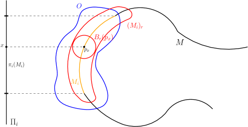
Figure 1. Proof of Proposition 2.14 in the case $d=2$ and $m=1$.

∎

2.8. Lipschitz sets and one-sided Minkowski contents

We start by recalling a basic property of Lipschitz sets.

Lemma 2.15.

Let $\Omega\subset\mathbb{R}^{d}$ be a bounded open set with Lipschitz boundary. Then, for $\mathcal{H}^{d-1}$ almost every $x\in\partial\Omega$ there exists a unit vector $n_{x}$ such that for any $\alpha\in(0,\nicefrac{{\pi}}{{2}})$ there exists $r_{\alpha}>0$ such that for any $r\in(0,r_{\alpha})$ it holds that

$$\{y\in B_{r}(x)\,\colon\,\langle y-x,-n_{x}\rangle>\cos(\alpha)\left|y-x\right|\}\subset\Omega,$$ (2.21)

$$\{y\in B_{r}(x)\,\colon\,\langle y-x,n_{x}\rangle>\cos(\alpha)\left|y-x\right|\}\subset\mathbb{R}^{d}\setminus\overline{\Omega}.$$ (2.22)

Remark 2.16.

Given an open set $\Omega$ with Lipschitz boundary, Lemma 2.15 establishes the existence, $\mathcal{H}^{d-1}\llcorner\partial\Omega$ almost everywhere, of a unit vector $n_{x}$ such that for any $\alpha\in(0,\nicefrac{{\pi}}{{2}})$ the cones of angle $\alpha$ around $-n_{x}$ and $n_{x}$ are contained in $\Omega$ and $\mathbb{R}^{d}\setminus\overline{\Omega}$ for small radii, respectively. Moreover, the vector $n_{x}$ is unique at any point at which it is defined and it plays the role of an outer unit normal vector.

Following the lines of the proof of Proposition 2.14, we establish the following result.

Proposition 2.17.

Let $\Omega\subset\mathbb{R}^{d}$ be a bounded open set with Lipschitz boundary and $\Sigma\subset\partial\Omega$ Borel. Then, for any $O\subset\mathbb{R}^{d}$ open it holds

$$\liminf_{r\rightarrow 0}\frac{\mathcal{H}^{d}\left((\Sigma)_{r}^{\rm in}\cap O\right)}{r}\geq\mathcal{H}^{d-1}(\Sigma\cap O)$$ (2.23)

and

$$\liminf_{r\rightarrow 0}\frac{\mathcal{H}^{d}\left((\Sigma)_{r}^{\rm out}\cap O\right)}{r}\geq\mathcal{H}^{d-1}(\Sigma\cap O).$$ (2.24)

Proof.

Fix an open set $O\subset\mathbb{R}^{d}$. We check the validity of (2.23) by following the proof of Proposition 2.14. The proof of (2.24) is analogous and thus left to the reader. By Proposition 2.13, it is enough to check that for any finite collection of pairwise disjoint compact sets $M_{1},\dots,M_{n}\subset\Sigma\cap O$ and for any $\Pi_{1},\dots,\Pi_{n}\in\mathbb{G}_{d-1}^{d}$ it holds that

$$\liminf_{r\to 0}\frac{\mathcal{H}^{d}\left((\Sigma)_{r}^{\rm in}\cap O\right)}{r}\geq\sum_{i=1}^{n}\mathcal{H}^{d-1}(\pi_{i}(M_{i})),$$ (2.25)

where we set $\pi_{i}=\pi_{\Pi_{i}}$. Since $M_{1},\dots,M_{n}$ are compact and disjoint, it is easy to check that

$$\liminf_{r\to 0}\frac{\mathcal{H}^{d}\left((\Sigma)_{r}^{\rm in}\cap O\right)}{r}\geq\sum_{i=1}^{n}\liminf_{r\to 0}\frac{\mathcal{H}^{d}\left((M_{i})_{r}^{\rm in}\cap O\right)}{r}.$$ (2.26)

Then, to prove (2.23) it suffices to check that

$$\liminf_{r\to 0}\frac{\mathcal{H}^{d}\left((M_{i})_{r}^{\rm in}\cap O\right)}{r}\geq\mathcal{H}^{d-1}(\pi_{i}(M_{i}))\qquad\forall i=1,\dots,n.$$ (2.27)

Given any $i\in\{1,\dots,n\}$, by Fubini’s theorem and Fatou’s lemma we get

$$\liminf_{r\to 0}\frac{\mathcal{H}^{d}\left((M_{i})_{r}^{\rm in}\cap O\right)}{r} =\liminf_{r\to 0}\int_{\Pi_{i}}\frac{\mathcal{H}^{1}\left((M_{i})_{r}^{\rm in}\cap O\cap\pi_{i}^{-1}(x)\right)}{r}\,d\mathcal{H}^{d-1}(x)$$ (2.28)

$$\geq\liminf_{r\to 0}\int_{\pi_{i}(M_{i})}\frac{\mathcal{H}^{1}\left((M_{i})_{r}^{\rm in}\cap O\cap\pi_{i}^{-1}(x)\right)}{r}\,d\mathcal{H}^{d-1}(x)$$ (2.29)

$$\geq\int_{\pi_{i}(M_{i})}\liminf_{r\to 0}\frac{\mathcal{H}^{1}\left((M_{i})_{r}^{\rm in}\cap O\cap\pi_{i}^{-1}(x)\right)}{r}\,d\mathcal{H}^{d-1}(x).$$ (2.30)

To conclude, it is enough to prove that for $\mathcal{H}^{d-1}$ almost every $x\in\pi_{i}(M_{i})$ it holds that

$$\liminf_{r\to 0}\frac{\mathcal{H}^{d-1}\left((M_{i})_{r}^{\rm in}\cap O\cap\pi_{i}^{-1}(x)\right)}{r}\geq 1.$$ (2.31)

With the notation of Lemma 2.15, we set

$$S_{i}:=\left\{x\in\pi_{i}(M_{i})\,\colon\,\exists p_{x}\in M_{i}\text{ s.t. $n_{p_{x}}$ is well defined and }n_{p_{x}}\notin\Pi_{i}\right\}.$$ (2.32)

We claim that $\mathcal{H}^{d-1}\left(\pi_{i}(M_{i})\cap S_{i}^{c}\right)=0$ and that (2.31) is satisfied for any $x\in S_{i}$. To begin, we notice that $\pi_{i}(M_{i})\cap S_{i}^{c}\subset\pi_{i}(A_{i})\cup\pi_{i}(B_{i})$, with

$$A_{i}=\{y\in M_{i}\,\colon\,n_{y}\text{ is not defined}\}\qquad\text{and}\qquad B_{i}=\{y\in M_{i}\,\colon\,n_{y}\text{ is defined and }n_{y}\in\Pi_{i}\}.$$

Since $\pi_{i}$ is $1$-Lipschitz and $n_{y}$ is defined for $\mathcal{H}^{d-1}$-a.e. $y\in\partial\Omega$, we infer that $\mathcal{H}^{d-1}(\pi_{i}(A_{i}))\leq\mathcal{H}^{d-1}(A_{i})=0$. Next, we prove that $\mathcal{H}^{d-1}(\pi_{i}(B_{i}))=0$. Recalling that $B_{i}$ is $(d-1)$-rectifiable, by the area formula with the tangential differential [AFP00]*Theorem 2.91, we have

$$\int_{\Pi_{i}}\mathcal{H}^{0}\left(B_{i}\cap\pi_{i}^{-1}(y)\right)\,d\mathcal{H}^{d-1}(y)=\int_{B_{i}}J_{d-1}^{B_{i}}\pi_{i}(y)\,d\mathcal{H}^{d-1}(y).$$ (2.33)

Here $J_{d-1}^{B_{i}}\pi_{i}(y)$ is the determinant of the differential of the restriction of $\pi_{i}$ to $y+\text{Tan}(y;B_{i})$, computed at $y$. We notice that

$$\mathcal{H}^{0}\left(B_{i}\cap\pi_{i}^{-1}(y)\right)\geq\mathds{1}_{\pi_{i}(B_{i})}(y)\qquad\forall y\in\Pi_{i},$$

thus proving

$$\mathcal{H}^{d-1}(\pi_{i}(B_{i}))\leq\int_{B_{i}}J_{d-1}^{B_{i}}\pi_{i}(y)\,d\mathcal{H}^{d-1}(y).$$ (2.34)

Moreover, for any $y\in B_{i}$, $\pi_{i}$ is constant along any line contained in the tangent space to $\partial\Omega$ at $y$. Thus, the determinant of the tangential Jacobian at $y$ vanishes. Therefore, we deduce

$$\int_{B_{i}}J_{d-1}^{B_{i}}\pi_{i}(y)\,d\mathcal{H}^{d-1}(y)=0,$$

yielding $\mathcal{H}^{d-1}(\pi_{i}(B_{i}))=0$. To conclude, pick any $x\in S_{i}$. We check that (2.31) is satisfied at $x$. Let $v_{i}$ be a unit vector such that $\Pi_{i}^{\perp}=\text{Span}(v_{i})$. Since $x\in S_{i}$ we can find $p\in M_{i}$ such that $\pi_{i}(p)=x$ and $n_{p}\notin\Pi_{i}$. Without loss of generality we can assume that $\langle n_{p},v_{i}\rangle>0$. Then, we can find an angle $\alpha_{p}\in(0,\nicefrac{{\pi}}{{2}})$ such that $0<\cos(\alpha_{p})<\langle n_{p},v_{i}\rangle$. Letting $r_{\alpha_{p}}$ as in Lemma 2.15, it is clear that for any $r<r_{\alpha_{p}}$ the segment between $p$ and $p+rv_{i}$ is contained in $(M_{i})^{\rm in}_{r}\cap\pi_{i}^{-1}(x)$. Since $O$ is an open set, the segment is also contained in $O$, possibly choosing a smaller $r_{\alpha_{p}}$. This proves (2.31) at $x$. ∎

Now, let us restrict to $\Sigma\subset\partial\Omega$ closed. We remark that by [ACA08]*Corollary 1 (see also the more general statement [ACA08]*Theorem 5) we also have the convergence of the total masses of the two sequences of measures defined as

$$\frac{\mathcal{H}^{d}\left((\Sigma)_{r}^{\rm in}\cap A\right)}{r}\qquad\text{and}\qquad\frac{\mathcal{H}^{d}\left((\Sigma)_{r}^{\rm out}\cap A\right)}{r}\qquad\qquad\forall A\subset\mathbb{R}^{d}\text{ Borel}.$$

Thus, with Proposition 2.17 in hand, by Proposition 2.2 we could directly conclude the weak convergence of the one-sided Minkowski contents as measures concentrated on $\Sigma$. However, in order to keep this note self-contained, the next corollary gives an independent and elementary proof of this fact.

Corollary 2.18.

Let $\Omega\subset\mathbb{R}^{d}$ be a bounded open set with Lipschitz boundary and $\Sigma\subset\partial\Omega$ closed. Then, as $r\rightarrow 0$, it holds that

$$\frac{\mathcal{H}^{d}\llcorner(\Sigma)_{r}^{\rm in}}{r}\rightharpoonup\mathcal{H}^{d-1}\llcorner\Sigma\qquad\text{and}\qquad\frac{\mathcal{H}^{d}\llcorner(\Sigma)_{r}^{\rm out}}{r}\rightharpoonup\mathcal{H}^{d-1}\llcorner\Sigma.$$

Proof.

We want to apply Proposition 2.2. Thanks to Proposition 2.17 we already have that both sequences of measures are lower semicontinuous on open sets. Thus, it suffices to check that their masses converge to $\mathcal{H}^{d-1}(\Sigma)$. We split

$$\frac{\mathcal{H}^{d}\left((\Sigma)_{r}\right)}{2{r}}=\frac{1}{2}\left(\frac{\mathcal{H}^{d}\left((\Sigma)_{r}^{\text{in}}\right)}{{r}}+\frac{\mathcal{H}^{d}\left((\Sigma)_{r}^{\text{out}}\right)}{{r}}\right).$$

By Proposition 2.12 and by applying (2.23) and (2.24) with $O=\mathbb{R}^{d}$ we deduce

$$\mathcal{H}^{d-1}(\Sigma)\leq\frac{1}{2}\left(\liminf_{r\rightarrow 0}\frac{\mathcal{H}^{d}\left((\Sigma)_{r}^{\text{in}}\right)}{{r}}+\liminf_{r\rightarrow 0}\frac{\mathcal{H}^{d}\left((\Sigma)_{r}^{\text{out}}\right)}{{r}}\right)\leq\mathcal{H}^{d-1}(\Sigma).$$

In particular

$$\liminf_{r\rightarrow 0}\frac{\mathcal{H}^{d}\left((\Sigma)_{r}^{\text{in}}\right)}{{r}}+\liminf_{r\rightarrow 0}\frac{\mathcal{H}^{d}\left((\Sigma)_{r}^{\text{out}}\right)}{{r}}=2\mathcal{H}^{d-1}(\Sigma),$$

which, by using again (2.23) and (2.24), necessarily implies

$$\liminf_{r\rightarrow 0}\frac{\mathcal{H}^{d}\left((\Sigma)_{r}^{\text{in}}\right)}{{r}}=\mathcal{H}^{d-1}(\Sigma)\qquad\text{and}\qquad\liminf_{r\rightarrow 0}\frac{\mathcal{H}^{d}\left((\Sigma)_{r}^{\text{out}}\right)}{{r}}=\mathcal{H}^{d-1}(\Sigma).$$

Since the above inferior limits are uniquely defined and do not depend on the choice of the sequence $r\rightarrow 0$, we conclude

$$\lim_{r\rightarrow 0}\frac{\mathcal{H}^{d}\left((\Sigma)_{r}^{\text{in}}\right)}{{r}}=\mathcal{H}^{d-1}(\Sigma)\qquad\text{and}\qquad\lim_{r\rightarrow 0}\frac{\mathcal{H}^{d}\left((\Sigma)_{r}^{\text{out}}\right)}{{r}}=\mathcal{H}^{d-1}(\Sigma).$$

∎

3. Normal Lebesgue trace: Gauss-Green and further properties

In this section we prove several properties of the normal Lebesgue trace, the most important being the Gauss-Green identity. In addition to their possible independent interest, such properties will be used in the proof of Theorem 1.6 and for a comparison with the previous results obtained in [CDS14].

3.1. Gauss-Green identity

Here we prove Theorem 1.4, together with several others properties relating integrals on tubular neighbourhoods to boundary integrals of traces, when the latter are suitably defined. Everything will follow from the next general proposition.

Proposition 3.1.

Let $f:\Omega\rightarrow\mathbb{R}$, $f\in L^{\infty}(\Omega)$, $\Omega\subset\mathbb{R}^{d}$ a bounded open set with Lipschitz boundary and $\Sigma\subset\partial\Omega$ closed. Assume that there exists $f^{\Sigma}:\Sigma\rightarrow\mathbb{R}$ such that

$$\lim_{r\rightarrow 0}\frac{1}{r^{d}}\int_{B_{r}(x)\cap\Omega}\left|f(y)-f^{\Sigma}(x)\right|\,dy=0\qquad\text{for }\mathcal{H}^{d-1}\text{-a.e. }x\in\Sigma.$$ (3.1)

Then, for any $\varphi\in C^{\infty}_{c}(\mathbb{R}^{d})$ it holds

$$\lim_{r\rightarrow 0}\frac{1}{r}\int_{(\Sigma)_{r}^{\rm in}}f\varphi\,dy=\int_{\Sigma}f^{\Sigma}\varphi\,d\mathcal{H}^{d-1}.$$ (3.2)

Remark 3.2.

If $f\in L^{\infty}(\Omega)$, the sequence of functions

$$\Sigma\ni x\mapsto\frac{1}{r^{d}}\int_{B_{r}(x)\cap\Omega}f(y)\,dy$$

is bounded in $L^{\infty}(\Sigma;\mathcal{H}^{d-1})$. Thus, $f^{\Sigma}\in L^{\infty}(\Sigma;\mathcal{H}^{d-1})$.

A direct corollary of Proposition 3.1 is the following.

Corollary 3.3.

Let $u:\Omega\rightarrow\mathbb{R}^{d}$, $u\in L^{\infty}(\Omega)$, $\Omega\subset\mathbb{R}^{d}$ a bounded open set with Lipschitz boundary and set

$$\chi_{r}(y):=\begin{cases}1&y\in\Omega\setminus(\partial\Omega)_{r}^{\rm in}\\ \frac{d_{\partial\Omega}(y)}{r}&y\in(\partial\Omega)_{r}^{\rm in}.\end{cases}$$ (3.3)

Assume that $u$ has an outward normal Lebesgue trace $u^{\partial\Omega}_{n}$ on $\partial\Omega$ according to Definition 1.3. Then, for any $\varphi\in C^{\infty}_{c}(\mathbb{R}^{d})$, it holds

$$\lim_{r\rightarrow 0}\int_{\Omega}\varphi u\cdot\nabla\chi_{r}\,dy=-\int_{\partial\Omega}\varphi u^{\partial\Omega}_{n}\,d\mathcal{H}^{d-1}.$$ (3.4)

Proof.

The left-hand side in (3.4) can be written as

$$\lim_{r\rightarrow 0}\frac{1}{r}\int_{(\partial\Omega)_{r}^{\rm in}}\varphi u\cdot\nabla d_{\partial\Omega}\,dy.$$

Thus, by applying Proposition 3.1 with $f=u\cdot\nabla d_{\partial\Omega}$, $f^{\Sigma}=u^{\partial\Omega}_{-n}$ and $\Sigma=\partial\Omega$, we obtain

$$\lim_{r\rightarrow 0}\int_{\Omega}\varphi u\cdot\nabla\chi_{r}\,dy=\int_{\partial\Omega}\varphi u^{\partial\Omega}_{-n}\,d\mathcal{H}^{d-1}.$$

The proof is concluded since $u^{\partial\Omega}_{-n}=-u^{\partial\Omega}_{n}$. ∎

Then, Theorem 1.4 directly follows.

Proof of Theorem 1.4.

Denote $\lambda:=\mathop{\rm div}\nolimits u$. Since $\varphi\chi_{r}\in\mathop{\rm Lip}\nolimits_{c}(\mathbb{R}^{d})$ and $\varphi\chi_{r}\big{|}_{\partial\Omega}\equiv 0$, by (1.1) we have

$$\int_{\Omega}\varphi\chi_{r}\,d\lambda+\int_{\Omega}\varphi u\cdot\nabla\chi_{r}\,dy+\int_{\Omega}\chi_{r}u\cdot\nabla\varphi\,dy=0.$$

Letting $r\rightarrow 0$, since $\Omega$ is open, we have

$$\int_{\Omega}\chi_{r}u\cdot\nabla\varphi\,dy\rightarrow\int_{\Omega}u\cdot\nabla\varphi\,dy\qquad\text{and}\qquad\int_{\Omega}\varphi\chi_{r}\,d\lambda\rightarrow\int_{\Omega}\varphi\,d\lambda.$$

Thus, by Corollary 3.3 we conclude

$$\int_{\Omega}\varphi\,d\lambda+\int_{\Omega}u\cdot\nabla\varphi\,dy=\int_{\partial\Omega}u^{\partial\Omega}_{n}\varphi\,d\mathcal{H}^{d-1}.$$

According to (1.1) the left hand side of the above equation equals $\int_{\partial\Omega}\mathop{\rm Tr}\nolimits_{n}(u;\partial\Omega)\varphi\,d\mathcal{H}^{d-1}$, which concludes the proof by the arbitrariness of $\varphi$. ∎

We are left to prove the key Proposition 3.1.

Proof of Proposition 3.1.

Let $\delta>0$ be fixed. By Lusin’s theorem we find a closed set $A_{1}\subset\Sigma$ such that $\mathcal{H}^{d-1}(\Sigma\setminus A_{1})<\frac{\delta}{2}$ and $f^{\Sigma}$ is continuous on $A_{1}$. Let $r_{k}\rightarrow 0$ be any sequence. By Egorov’s theorem, we find $A_{2}\subset\Sigma$, with $\mathcal{H}^{d-1}(\Sigma\setminus A_{2})<\frac{\delta}{2}$, such that the convergence in (3.1) is uniform on $A_{2}$. To sum up, by setting $A:=A_{1}\cap A_{2}\subset\Sigma$ we have

$$\mathcal{H}^{d-1}(\Sigma\setminus A)<\delta,$$ (3.5)

$f^{\Sigma}$ is continuous on $A$ and there exists $k_{0}\in\mathbb{N}$ such that for any $k>k_{0}$ and for any $x\in A$ it holds

$$\frac{1}{r_{k}^{d}}\int_{\Omega\cap B_{5r_{k}}(x)}\left|f(y)-f^{\Sigma}(x)\right|\,dy<\delta.$$ (3.6)

By Tietze extension theorem we find a continuous function $\tilde{f}^{\Sigma}:\partial\Omega\rightarrow\mathbb{R}$ such that $\tilde{f}^{\Sigma}\equiv f^{\Sigma}$ on $A$ and $\|\tilde{f}^{\Sigma}\|_{L^{\infty}(\partial\Omega)}\leq\left\|f^{\Sigma}\right\|_{L^{\infty}(\Sigma)}$. Since $\partial\Omega$ is compact, $\tilde{f}^{\Sigma}$ is uniformly continuous. Denote by $\tilde{\gamma}$ its modulus of continuity. Let $\varphi\in C^{\infty}_{c}(\mathbb{R}^{d})$ be any test function. Then, by using the projection onto $\partial\Omega$ defined in Lemma 2.10, we split the integral

$$\left|\frac{1}{r_{k}}\int_{(\Sigma)^{\rm in}_{r_{k}}}\varphi f\,dy-\int_{\Sigma}\varphi f^{\Sigma}\,d\mathcal{H}^{d-1}\right|\leq \left\|\varphi\right\|_{L^{\infty}(\mathbb{R}^{d})}\int_{\Sigma}\left|f^{\Sigma}-\tilde{f}^{\Sigma}\right|\,d\mathcal{H}^{d-1}$$ (3.7)

$$+\left|\frac{1}{r_{k}}\int_{(\Sigma)^{\rm in}_{r_{k}}}\varphi\tilde{f}^{\Sigma}\circ\pi_{\partial\Omega}\,dy-\int_{\Sigma}\varphi\tilde{f}^{\Sigma}\,d\mathcal{H}^{d-1}\right|$$ (3.8)

$$+\frac{\left\|\varphi\right\|_{L^{\infty}(\mathbb{R}^{d})}}{r_{k}}\int_{(\Sigma)^{\rm in}_{r_{k}}\setminus(A)_{r_{k}}}\left|f-\tilde{f}^{\Sigma}\circ\pi_{\partial\Omega}\right|\,dy$$ (3.9)

$$+\frac{\left\|\varphi\right\|_{L^{\infty}(\mathbb{R}^{d})}}{r_{k}}\int_{(\Sigma)^{\rm in}_{r_{k}}\cap(A)_{r_{k}}}\left|f-\tilde{f}^{\Sigma}\circ\pi_{\partial\Omega}\right|\,dy$$ (3.10)

$$= I_{k}+II_{k}+III_{k}+IV_{k}.$$ (3.11)

By (3.5) together with Remark 3.2 we have

$$I_{k}\lesssim\mathcal{H}^{d-1}(\Sigma\setminus A)\left\|f^{\Sigma}\right\|_{L^{\infty}(\Sigma)}\lesssim\delta.$$ (3.12)

Moreover, Lemma 2.10 implies that $\tilde{f}^{\Sigma}\circ\pi_{\partial\Omega}$ is continuous on $\partial\Omega$. Thus, by Corollary 2.18 and Proposition 2.3 we deduce $\lim_{k\to\infty}II_{k}=0$. Note that here we are allowed to apply Proposition 2.3 since our sequence of measures is concentrated on compact sets, thus the two notions of convergence (2.2) and (2.1) are equivalent.

To estimate $III_{k}$, since both $\Sigma$ and $A$ are closed $(d-1)$-rectifiable sets, by Proposition 2.12 it holds that

$$\lim_{r\to 0}\frac{\mathcal{H}^{d}((\Sigma)_{r})}{\omega_{1}r}=\mathcal{H}^{d-1}(\Sigma)\qquad\text{ and }\qquad\lim_{r\to 0}\frac{\mathcal{H}^{d}((A)_{r})}{\omega_{1}r}=\mathcal{H}^{d-1}(A).$$ (3.13)

Thus, we infer that

$$\lim_{r\to 0}\frac{\mathcal{H}^{d}((\Sigma)_{r}\setminus(A)_{r})}{\omega_{1}r}=\mathcal{H}^{d-1}(\Sigma\setminus A)<\delta,$$ (3.14)

from which we deduce

$$\limsup_{k\to\infty}III_{k}\lesssim\limsup_{k\to\infty}\frac{\mathcal{H}^{d}\left((\Sigma)^{\rm in}_{r_{k}}\setminus(A)_{r_{k}}\right)}{r_{k}}\lesssim\limsup_{k\to\infty}\frac{\mathcal{H}^{d}((\Sigma)_{r_{k}}\setminus(A)_{r_{k}})}{r_{k}}\lesssim\delta.$$ (3.15)

We are left with $IV_{k}$. By Vitali’s covering lemma we find a disjoint family of balls $\{B_{r}(x_{j})\}_{j\in J}$ such that $x_{j}\in A$ for any $j\in J$ and

$$(A)_{r}\subset\bigcup_{j\in J}B_{5r}(x_{j}).$$

Since the Minkowski dimension of $\partial\Omega$ is $d-1$, for sufficiently small radii $r$ it must hold that

$$\#J\lesssim r^{1-d}.$$ (3.16)

Then, recalling that $\tilde{f}^{\Sigma}=f^{\Sigma}$ on $A\subset\Sigma$, we have that

$$IV_{k} \lesssim\frac{1}{r_{k}}\sum_{j\in J}\int_{\Omega\cap B_{5r_{k}}(x_{j})}\left|f(y)-\tilde{f}^{\Sigma}(\pi_{\partial\Omega}(y))\right|\,dy$$ (3.17)

$$\leq\frac{1}{r_{k}}\sum_{j\in J}\int_{\Omega\cap B_{5r_{k}}(x_{j})}\left|f(y)-f^{\Sigma}(x_{j})\right|\,dy+\frac{1}{r_{k}}\sum_{j\in J}\int_{\Omega\cap B_{5r_{k}}(x_{j})}\left|\tilde{f}^{\Sigma}(x_{j})-\tilde{f}^{\Sigma}(\pi_{\partial\Omega}(y))\right|\,dy$$ (3.18)

$$=IV^{1}_{k}+IV^{2}_{k}.$$ (3.19)

By (3.6) and (3.16), for $k>k_{0}$ we infer that $IV^{1}_{k}\lesssim\#J\delta r_{k}^{d-1}\lesssim\delta$. For any $j\in J$ and for almost every $y\in B_{5r_{k}}(x_{j})\cap\Omega$, by the minimality of $\pi_{\partial\Omega}(y)$ we get

$$\left|\pi_{\partial\Omega}(y)-x_{j}\right|\leq\left|\pi_{\partial\Omega}(y)-y\right|+\left|y-x_{j}\right|\leq 2\left|y-x_{j}\right|\leq 10r_{k},$$

from which, recalling that $\tilde{\gamma}$ is the modulus of continuity of $\tilde{f}^{\Sigma}$, we deduce

$$IV_{k}^{2}\lesssim\frac{\#J}{r_{k}}\tilde{\gamma}(10r_{k})\mathcal{H}^{d}(B_{5r_{k}})\lesssim\tilde{\gamma}(10r_{k}).$$ (3.20)

Thus, we achieved

$$\limsup_{k\to\infty}IV_{k}\lesssim\lim_{k\to\infty}\tilde{\gamma}(10r_{k})+\delta\lesssim\delta.$$ (3.21)

To summarize, we have shown that

$$\limsup_{k\to\infty}\left|\frac{1}{r_{k}}\int_{(\Sigma)^{\rm in}_{r_{k}}}\varphi f\,dy-\int_{\Sigma}\varphi f^{\Sigma}\,d\mathcal{H}^{d-1}\right|\lesssim\delta.$$ (3.22)

The conclusion immediately follows since both $r_{k}\rightarrow 0$ and $\delta>0$ are arbitrary. ∎

Since it might be of independent interest, we also state the following result, which in turn generalizes [DRINV23]*Proposition 5.3.

Corollary 3.4.

Let $u\in L^{\infty}(\Omega)$ be a vector field, $\Omega\subset\mathbb{R}^{d}$ a bounded open set with Lipschitz boundary and let $\chi_{r}$ be as in (3.3). Assume that $u$ has an outward normal Lebesgue trace $u^{\partial\Omega}_{n}$ on $\partial\Omega$ according to Definition 1.3. Then, for any $\varphi\in C^{\infty}_{c}(\mathbb{R}^{d})$, it holds

$$\lim_{r\rightarrow 0}\int_{\Omega}\varphi\left|u\cdot\nabla\chi_{r}\right|\,dy=\int_{\partial\Omega}\varphi\left|u^{\partial\Omega}_{n}\right|\,d\mathcal{H}^{d-1}.$$ (3.23)

Notice that

$$\frac{1}{r^{d}}\int_{B_{r}(x)\cap\Omega}\left||u\cdot\nabla d_{\partial\Omega}|-|u_{-n}^{\partial\Omega}(x)|\right|\,dy\leq\frac{1}{r^{d}}\int_{B_{r}(x)\cap\Omega}\left|u\cdot\nabla d_{\partial\Omega}-u_{-n}^{\partial\Omega}(x)\right|\,dy.$$

Thus, Corollary 3.4 follows again by Proposition 3.1. By recalling the notion of traces for $BV$ functions from Theorem 2.4, we also get the following corollary, which will be useful later on in Section 4.

Corollary 3.5.

Let $\Omega\subset\mathbb{R}^{d}$ be a bounded open set with Lipschitz boundary and let $f\in BV(\Omega)\cap L^{\infty}(\Omega)$. Let $\Sigma\subset\partial\Omega$ be a closed set. Then, it holds

$$\lim_{r\to 0}\frac{1}{r}\int_{(\Sigma)_{r}^{\rm in}}f\,dx=\int_{\Sigma}f^{\Omega}\,d\mathcal{H}^{d-1}.$$ (3.24)

3.2. Positive and negative normal Lebesgue traces

We start by specifying how Definition 1.3 trivially extends to the case in which only a portion of the boundary $\Sigma\subset\partial\Omega$ is considered.

Definition 3.6.

Let $\Omega\subset\mathbb{R}^{d}$ be a bounded Lipschitz open set, $\Sigma\subset\partial\Omega$ measurable and $u\in L^{1}(\Omega)$ a vector field. We say that $u$ admits an inward Lebesgue normal trace on $\Sigma$ if there exists a function $f\in L^{1}(\Sigma;\mathcal{H}^{d-1})$ such that, for every sequence $r_{k}\rightarrow 0$, it holds

$$\lim_{k\rightarrow\infty}\frac{1}{r_{k}^{d}}\int_{B_{r_{k}}(x)\cap\Omega}\left|(u\cdot\nabla d_{\partial\Omega})(y)-f(x)\right|\,dy=0\qquad\text{for }\mathcal{H}^{d-1}\text{-a.e. }x\in\Sigma.$$

Whenever such a function exits, we will denote it by $f=:u_{-n}^{\Sigma}$. Consequently, the outward Lebesgue normal trace on $\Sigma$ will be $u_{n}^{\Sigma}:=-u_{-n}^{\Sigma}$.

Even if the definition is given on a general measurable set $\Sigma\subset\partial\Omega$, the meaningful case is $\mathcal{H}^{d-1}(\Sigma)>0$.

Remark 3.7.

The same definition can be given for any oriented Lipschitz hypersurfaces $\Sigma\subset\mathbb{R}^{d}$. In the case $\Sigma\subset\partial\Omega$, an orientation is canonically induced on $\Sigma$. Since it will be sufficient for our purposes, we will only deal with such a case.

It is rather easy to show that the positive and negative part of the normal Lebesgue trace behave well as soon as the latter exists. Indeed, if $f_{+}$ and $f_{-}$ are the positive and the negative part of a function $f$, that is $f=f_{+}-f_{-}$, from $|f_{-}-g_{-}|,|f_{+}-g_{+}|\leq|f-g|$ we immediately obtain the following result.

Proposition 3.8.

Let $\Omega\subset\mathbb{R}^{d}$ be a bounded Lipschitz open set, $\Sigma\subset\partial\Omega$ be measurable, $u\in L^{1}(\Omega)$ a vector field which has a normal Lebesgue trace $u^{\Sigma}_{n}$ according to Definition 3.6. Then, for every sequence $r_{k}\rightarrow 0$, we have

$$\lim_{k\rightarrow\infty}\frac{1}{r_{k}^{d}}\int_{B_{r_{k}}(x)\cap\Omega}\left|(u\cdot\nabla d_{\partial\Omega})_{+}(y)-\left(u^{\Sigma}_{-n}\right)_{+}(x)\right|\,dy=0\qquad\text{for }\mathcal{H}^{d-1}\text{-a.e. }x\in\Sigma$$

and

$$\lim_{k\rightarrow\infty}\frac{1}{r_{k}^{d}}\int_{B_{r_{k}}(x)\cap\Omega}\left|(u\cdot\nabla d_{\partial\Omega})_{-}(y)-\left(u^{\Sigma}_{-n}\right)_{-}(x)\right|\,dy=0\qquad\text{for }\mathcal{H}^{d-1}\text{-a.e. }x\in\Sigma.$$

As an almost direct consequence we have the following result.

Corollary 3.9.

Let $\Omega\subset\mathbb{R}^{d}$ be a bounded open set with Lipschitz boundary, $\Sigma\subset\partial\Omega$ be measurable, $u\in L^{\infty}(\Omega)$ a vector field which has an outward normal Lebesgue trace $u^{\Sigma}_{n}$. The following facts are true.

• If $\tilde{\Sigma}\subset\Sigma$ is any closed set on which $u^{\Sigma}_{n}\big{|}_{\tilde{\Sigma}}\geq 0$, we have

  $$\lim_{r\rightarrow 0}\frac{1}{r}\int_{(\tilde{\Sigma})^{\rm in}_{r}}(u\cdot\nabla d_{\partial\Omega})_{+}(y)\,dy=0.$$ (3.25)

• If $\tilde{\Sigma}\subset\Sigma$ is any closed set on which $u^{\Sigma}_{n}\big{|}_{\tilde{\Sigma}}\leq 0$, we have

  $$\lim_{r\rightarrow 0}\frac{1}{r}\int_{(\tilde{\Sigma})^{\rm in}_{r}}(u\cdot\nabla d_{\partial\Omega})_{-}(y)\,dy=0.$$

Restricting to closed subsets of $\Sigma$ in the above result is necessary. Even if $u^{\Sigma}_{n}$ has distinguished sign on $\Sigma$, we can not expect the conclusions of Corollary 3.9 to hold replacing $\tilde{\Sigma}$ by $\Sigma$. Indeed, $\Sigma$ could be countable and dense in $\partial\Omega$, from which $(\Sigma)_{r}=(\partial\Omega)_{r}$ for any $r>0$, but it is clear that any assumption on a $\mathcal{H}^{d-1}$-negligible subset of $\partial\Omega$ will not suffice to deduce anything in the whole $(\partial\Omega)_{r}$.

Proof.

Since $u^{\Sigma}_{-n}\big{|}_{\tilde{\Sigma}}=-u^{\Sigma}_{n}\big{|}_{\tilde{\Sigma}}\leq 0$, by Proposition 3.8 we deduce

$$\lim_{k\rightarrow\infty}\frac{1}{r_{k}^{d}}\int_{B_{r_{k}}(x)\cap\Omega}(u\cdot\nabla d_{\partial\Omega})_{+}(y)\,dy=0\qquad\text{for }\mathcal{H}^{d-1}\text{-a.e. }x\in\tilde{\Sigma}.$$

Then, (3.25) follows by applying Proposition 3.1 with $f=(u\cdot\nabla d_{\partial\Omega})_{+}$, $f^{\tilde{\Sigma}}=0$ and $\varphi=1$. The proof of $(ii)$ is completely analogous. ∎

We conclude this section by showing that $BV$ vector fields satisfy (3.25) with $\tilde{\Sigma}$ being the portion of the boundary where $u$ is pointing outward. In particular, this shows that our assumption (1.3) automatically holds if the vector field $u$ is $BV$ up to the boundary. Thus Theorem 1.6 offers an honest generalization of [CDS14]. In some sense, and as expected, the next proposition shows that $BV$ vector fields achieve the positive and negative values of their normal trace in a uniform integral sense.

Proposition 3.10.

Let $\Omega\subset\mathbb{R}^{d}$ be a bounded open set with Lipschitz boundary and let $u\in BV(\Omega)\cap L^{\infty}(\Omega)\subset\mathcal{MD}^{\infty}(\Omega)$. We set

$$\Sigma^{+}:=\left\{x\in\partial\Omega\,:\,\mathop{\rm Tr}\nolimits_{n}(u;\partial\Omega)(x)\geq 0\right\}\qquad\text{and}\qquad\Sigma^{-}:=\partial\Omega\setminus\Sigma^{+}.$$

Then

$$\lim_{r\rightarrow 0}\frac{1}{r}\int_{(\tilde{\Sigma})^{\rm in}_{r}}(u\cdot\nabla d_{\partial\Omega})_{+}(y)\,dy=0\qquad\forall\tilde{\Sigma}\subset\Sigma^{+}\text{ closed}$$ (3.26)

and

$$\lim_{r\rightarrow 0}\frac{1}{r}\int_{(\tilde{\Sigma})^{\rm in}_{r}}(u\cdot\nabla d_{\partial\Omega})_{-}(y)\,dy=0\qquad\forall\tilde{\Sigma}\subset\Sigma^{-}\text{ closed}.$$ (3.27)

Proof.

Since $u\in BV(\Omega)$, by [DRINV23]*Proposition 5.5 we deduce that $u$ admits a normal Lebesgue trace $u^{\partial\Omega}_{n}$ in the sense of Definition 1.3. Moreover, Theorem 1.4 implies that $u^{\partial\Omega}_{n}\big{|}_{\Sigma^{+}}\geq 0$, from which (3.26) directly follows by applying Corollary 3.9. The proof of (3.27) is completely analogous. ∎

The global $BV(\Omega)$ assumption could have been relaxed to hold only locally around $\Sigma^{+}$ and $\Sigma^{-}$, possibly also up to a negligible subset of the boundary.

3.3. Lebesgue traces are strictly stronger than distributional traces

In this section we provide an example of a $2$-dimensional bounded divergence-free vector field which has zero normal distributional trace, but does not admit a normal Lebesgue trace. Denote by $\{e_{1},e_{2}\}$ the canonical orthonormal basis of $\mathbb{R}^{2}$. Consider the square $Q:=\{(x,y)\in\mathbb{R}^{2}:0\leq x<1,\ 1\leq y<2\}$ and its rescaled and translated copies

$$Q_{i,j}:=2^{-j}(Q+ie_{1})=\left\{(x,y)\in\mathbb{R}^{2}\,\colon\,\frac{i}{2^{j}}\leq x<\frac{i+1}{2^{j}},\ 2^{-j}\leq y<2^{-j+1}\right\},\qquad\forall i,j\in\mathbb{Z}.$$

Notice that this family of squares tiles the upper half-plane $\mathbb{R}^{2}_{+}$ (see Figure 2).

Figure 2. The “tiles” $Q_{i,j}$ become finer approaching the axis $\{y=0\}$.

Take any (possibly smooth) bounded divergence-free vector field $v:Q\to\mathbb{R}^{2}$ tangent to $\partial Q$, define the corresponding rescaled vector fields $v_{i,j}:Q_{i,j}\to\mathbb{R}^{2}$ as

$$v_{i,j}(x,y):=v(2^{j}x-i,2^{j}y)$$

and combine them to get $u:\mathbb{R}^{2}_{+}\to\mathbb{R}^{2}$ by setting $u=v_{i,j}$ on each $Q_{i,j}$. We establish some properties of this vector field. In the lemma below we will denote by $\mathop{\rm Tr}\nolimits_{n}(u;\partial\Omega)$ the distributional normal trace on $\partial\Omega$ according to Definition 1.2.

Lemma 3.11.

The vector field $u:\mathbb{R}^{2}_{+}\to\mathbb{R}^{2}$ defined above satisfies the following properties:

• $u$ is bounded, divergence-free and $\mathop{\rm Tr}\nolimits_{n}(u;\partial\mathbb{R}^{2}_{+})\equiv 0$;

• the restriction of $u$ to the strip $\{0<y<2^{-k}\}$ is $2^{-k-1}$-periodic in the first variable;

• for any $(\bar{x},0)\in\partial\mathbb{R}^{2}_{+}$ it holds that

  $$\liminf_{r\to 0}\frac{1}{r^{2}}\int_{B_{r}^{+}((\bar{x},0))}\left|u\cdot e_{2}\right|\,dx\,dy\geq\frac{1}{8}\int_{Q}\left|v\cdot e_{2}\right|\,dx\,dy.$$ (3.28)

In particular, if $v$ satisfies

$$\int_{Q}|v\cdot e_{2}|\,dx\,dy>0,$$ (3.29)

then $u$ does not admit a normal Lebesgue trace on $\partial\mathbb{R}^{2}_{+}=\mathbb{R}$ in the sense of Definition 1.3.

Proof.

Since $v$ is bounded, the same holds for $u$. Given $\varphi\in C^{1}_{c}(\mathbb{R}^{2})$ we compute

$$\int_{\mathbb{R}^{2}_{+}}u(x,y)\cdot\nabla\varphi(x,y)\,dx\,dy=\sum_{i,j\in\mathbb{Z}}\int_{Q_{i,j}}v_{i,j}\cdot\nabla\varphi\,dx\,dy$$

and since $v_{i,j}$ is divergence-free

$$\int_{\mathbb{R}^{2}_{+}}u(x,y)\cdot\nabla\varphi(x,y)\,dx\,dy=\sum_{i,j\in\mathbb{Z}}\int_{\partial Q_{i,j}}\varphi\,v_{i,j}\cdot n_{Q_{i,j}}\,d\mathcal{H}^{1}=0,$$

where in the last equality we have used that $v_{i,j}$ is tangent to $\partial Q_{i,j}$ since $v$ is tangent to $\partial Q$. This computation shows that $u$ is divergence-free (for this it would have been enough to test with $\varphi\in C^{1}_{c}(\mathbb{R}^{2}_{+})$) and that the normal distributional trace vanishes according to Definition 1.2, thus proving $(i)$.

To check $(ii)$ it is enough to prove that the restriction of $u$ to the strip $\{2^{-k-1}\leq y<2^{-k}\}$ is $2^{-k-1}$-periodic in the first variable. This is evident, since a point $(x,y)$ in this strip belongs to some square $Q_{i,k+1}$ and hence

$$u(x+2^{-k-1},y) =v_{i+1,k+1}(x+2^{-k-1},y)=v(2^{k+1}x-1-i+1,2^{k+1}y)$$ (3.30)

$$=v(2^{k+1}x-i,2^{k+1}y)=v_{i,k+1}(x,y)=u(x,y).$$ (3.31)

We are left with $(iii)$. Notice that in this case $\nabla d_{\partial\mathbb{R}^{2}_{+}}(x,y)=e_{2}$ for any $(x,y)\in\mathbb{R}^{2}_{+}$. Hence, given $(\bar{x},0)\in\partial\mathbb{R}^{2}_{+}$, for $2^{-k}\leq r<2^{-k+1}$ one can estimate

$$\frac{1}{r^{2}}\int_{B^{+}_{r}((\bar{x},0))}|u\cdot e_{2}|\,dx\,dy \geq 4^{k-1}\int_{B^{+}_{2^{-k}}((\bar{x},0))}|u\cdot e_{2}|\,dx\,dy$$ (3.32)

$$\geq 4^{k-1}\int_{[\bar{x}-2^{-k-1},\bar{x}+2^{-k-1}]\times[0,2^{-k-1}]}|u\cdot e_{2}|\,dx\,dy.$$ (3.33)

By exploiting the periodicity with respect to the first variable ($u$ is $2^{-k-2}$-periodic in $x$ in the strip $0<y<2^{-k-1}$), we get

$$4^{k-1} \int_{[\bar{x}-2^{-k-1},\bar{x}+2^{-k-1}]\times[0,2^{-k-1}]}\left|u\cdot e_{2}\right|\,dx\,dy=4^{k-1}\int_{[0,2^{-k}]\times[0,2^{-k-1}]}\left|u\cdot e_{2}\right|\,dx\,dy$$ (3.34)

$$=4^{k-1}\sum_{j\geq k+2}\sum_{i=0}^{2^{j-k}-1}\int_{Q_{i,j}}\left|v_{i,j}\cdot e_{2}\right|\,dx\,dy=4^{k-1}\sum_{j\geq k+2}\sum_{i=0}^{2^{j-k}-1}4^{-j}\int_{Q}\left|v\cdot e_{2}\right|\,dx\,dy$$ (3.35)

$$=\int_{Q}\left|v\cdot e_{2}\right|\,dx\,dy\sum_{j\geq k+2}2^{k-j-2}=\frac{1}{8}\int_{Q}\left|v\cdot e_{2}\right|\,dx\,dy.$$ (3.36)

thus proving (3.28). To conclude, by Theorem 1.4, we know that if $u$ admits a normal Lebesgue trace, then it has to vanish. In particular, if $v$ satisfies (3.29), by (3.28) we infer that $u$ does not admit a normal Lebesgue trace on $\partial\mathbb{R}^{2}_{+}$. ∎

Remark 3.12.

For completeness we give an explicit example of a vector field $v$ satisfying the assumptions of Lemma 3.11 and (3.29). Let us define

$$v(x,y)=\Big{(}\sin(2\pi x)\cos(2\pi y),-\sin(2\pi y)\cos(2\pi x)\Big{)}.$$

It is apparent that $v$ is divergence-free, tangent to $\partial Q$ and

$$\int_{Q}|v\cdot e_{2}|\,dx\,dy=\int_{0}^{1}\int_{1}^{2}|\sin(2\pi y)\cos(2\pi x)|\,dx\,dy=\frac{4}{\pi^{2}}>0.$$

4. On the continuity equation on bounded domains

We now give the precise definition of weak solutions to the continuity equation (1.2). We follow [CDS14, CDS14bis]. For a regular solution $\rho$ to (1.2), testing the equation with $\varphi\in C^{1}(\overline{\Omega}\times[0,T))$, we get

$$\int_{0}^{T}\int_{\Omega}\rho(\partial_{t}\varphi+u\cdot\nabla\varphi)+(c\rho+f)\varphi\,dx\,dt=\int_{0}^{T}\int_{\partial\Omega}\rho u\cdot n_{\Omega}\varphi\,d\mathcal{H}^{d-1}\,dt-\int_{\Omega}\rho(x,0)\varphi(x,0)\,dx.$$ (4.1)

We aim to give meaning to the integral formulation (4.1) for rough solutions. To prescribe the boundary condition of $\rho$ on $\partial\Omega$, we exploit the theory of normal distributional traces. Let $u,\rho,c,f$ as in Theorem 1.6 and let $\rho\in L^{\infty}(\Omega\times(0,T))$ be an “interior in $\Omega$” distributional solution to

$$\left\{\begin{array}[]{rcll}\partial_{t}\rho+\mathop{\rm div}\nolimits(\rho u)&=&c\rho+f&\text{ in }\Omega\times(0,T)\\ \rho(\cdot,0)&=&\rho_{0}&\text{ in }\Omega,\end{array}\right.$$ (4.2)

that is, we restrict (4.1) to test functions in $C^{\infty}_{c}([0,T)\times\Omega)$. Thus, for the moment, we are not interested in the boundary datum on $\partial\Omega$. Moreover, setting $U=(u,1)$, we notice that the space-time divergence of $\rho U$ satisfies

$$\mathop{\rm Div}\nolimits(\rho U)=\mathop{\rm div}\nolimits(\rho u)+\partial_{t}\rho=c\rho+f,$$ (4.3)

that is $\rho U\in\mathcal{MD}^{\infty}(\Omega\times(0,T))$ and, recalling (1.1), we can define

$$\mathop{\rm Tr}\nolimits_{n}(\rho U;\partial(\Omega\times(0,T)))\in L^{\infty}(\partial(\Omega\times(0,T))).$$

We remark that the latter is a space-time normal trace. Indeed, for any fixed time $t\in(0,T)$, the vector field $\rho(\cdot,t)u(\cdot,t)$ might fail to belong to $\mathcal{MD}^{\infty}(\Omega)$. Thus, we need to consider the restriction of the space-time trace to $\Lambda:=\partial\Omega\times(0,T)$, that is

$$\mathop{\rm Tr}\nolimits_{n}(\rho u):=\mathop{\rm Tr}\nolimits_{n}(\rho U;\partial(\Omega\times(0,T)))\big{|}_{\Lambda}.$$ (4.4)

Similarly, we define

$$\mathop{\rm Tr}\nolimits_{n}(u):=\mathop{\rm Tr}\nolimits_{n}(U;\partial(\Omega\times(0,T)))\big{|}_{\Lambda}.$$ (4.5)

In this case, since $u(\cdot,t)\in\mathcal{MD}^{\infty}(\Omega)$ for a.e. $t$ (recall that we are assuming $\mathop{\rm div}\nolimits u\in L^{1}(\Omega\times(0,T))$), the normal trace at fixed time of $u$ is well defined and it can be checked that $\mathop{\rm Tr}\nolimits_{n}(u(\cdot,t);\partial\Omega)=\mathop{\rm Tr}\nolimits_{n}(u)(\cdot,t)$ for a.e. $t$ as functions in $L^{\infty}(\partial\Omega)$ (see Lemma A.1). Since the outer normal to the set $\Omega\times(0,T)$ is given by the vector $(n_{\Omega},0)$ at any point of $\Lambda$, then the traces $\mathop{\rm Tr}\nolimits_{n}(u)$ and $\mathop{\rm Tr}\nolimits_{n}(\rho u)$ describe the components of $u$ and $\rho u$ (respectively) which are normal to $\partial\Omega$.

Definition 4.1.

With the above notation, we define the space-time set where $u$ is not entering the domain $\Omega$ by

$$\widetilde{\Gamma}^{+}:=\left\{(x,t)\in\Lambda\,:\,\mathop{\rm Tr}\nolimits_{n}(u)(x,t)\geq 0\right\}.$$

We define $\Gamma^{+}:=\mathop{\rm Spt}\nolimits(\mathcal{H}^{d}\llcorner\widetilde{\Gamma}^{+})$. Then, the set where $u$ is entering $\Omega$ is defined by $\Gamma^{-}:=\Lambda\setminus\Gamma^{+}\subset\Lambda$.

Remark 4.2.

In Definition 4.1, the set $\widetilde{\Gamma}^{+}$ is defined up to $\mathcal{H}^{d}$-negligible sets. Then, we replace it with the closed (in $\Lambda$) representative given by $\Gamma^{+}$ for convenience. Hence, the set $\Gamma^{-}$ is open in $\Lambda$. We remark that $\Gamma^{+}$ is independent of the choice of the representative of $\mathop{\rm Tr}\nolimits_{n}(u)$. In view of the assumption $(i)$ in Theorem 1.6, if we set $\Gamma^{\pm}$ as in Definition 4.1, $\Gamma^{-}$ is the smallest subset of $\Lambda$ around which additional regularity of the vector field is assumed.

We notice that in the regular setting, we would have

$$\rho=\frac{(\rho u)\cdot n_{\Omega}}{u\cdot n_{\Omega}}=\frac{\mathop{\rm Tr}\nolimits_{n}(\rho u)}{\mathop{\rm Tr}\nolimits_{n}(u)},$$

provided $u\cdot n\neq 0$. Then, the idea is to impose the validity of the above formula to make sense of the boundary datum in the rough setting. Motivated by the discussion above, we recall the definition of weak solution to the initial-boundary value problem (1.2) from [CDS14, CDS14bis].

Definition 4.3.

Given $u,c,f,\rho_{0},g$ as in Theorem 1.6, we say that $\rho$ solves the continuity equation (1.2) with boundary condition $\rho=g$ on $\Gamma^{-}$ and initial datum $\rho_{0}$, if for any $\varphi\in C^{1}_{c}\left(\overline{\Omega}\times[0,T)\right)$

$$\int_{0}^{T}\int_{\Omega}\rho(\partial_{t}\varphi+u\cdot\nabla\varphi)+(c\rho+f)\varphi\,dx\,dt=\int_{0}^{T}\int_{\partial\Omega}\mathop{\rm Tr}\nolimits_{n}(\rho u)\varphi\,d\mathcal{H}^{d-1}\,dt-\int_{\Omega}\rho_{0}(x)\,\varphi(x,0)\,dx$$

and $\mathop{\rm Tr}\nolimits_{n}(\rho u)=g\mathop{\rm Tr}\nolimits_{n}(u)$ on $\Gamma^{-}$, where $\mathop{\rm Tr}\nolimits_{n}(\rho u),\mathop{\rm Tr}\nolimits_{n}(u)$ and $\Gamma^{-}$ are defined by (4.4), (4.5) and Definition 4.1.

By the interior renormalization property established in [Ambr04], under the assumptions of Theorem 1.6, for any choice of $\beta\in C^{1}(\mathbb{R})$, in the above notation, we have that

$$\mathop{\rm Div}\nolimits(\beta(\rho)U)=\mathop{\rm div}\nolimits(\beta(\rho)u)+\partial_{t}(\beta(\rho))=c\rho\beta^{\prime}(\rho)+f\beta^{\prime}(\rho)+(\beta(\rho)-\rho\beta^{\prime}(\rho))\mathop{\rm div}\nolimits u,$$ (4.6)

in $\mathcal{D}^{\prime}(\Omega\times(0,T))$. Hence, $\beta(\rho)U\in\mathcal{MD}^{\infty}(\Omega\times(0,T))$ and we set

$$\mathop{\rm Tr}\nolimits_{n}(\beta(\rho)u):=\mathop{\rm Tr}\nolimits_{n}(\beta(\rho)U;\partial(\Omega\times(0,T)))\big{|}_{\Lambda}\in L^{\infty}(\Lambda).$$ (4.7)

We prove a chain rule for the distributional normal trace of weak solutions to (1.2). The proof follows closely that of [ACM05]*Theorem 4.2 and relies on the Gagliardo extension theorem [Ga57] (see also [Le17]*Theorem 18.15 for a modern reference).

Proposition 4.4.

Under the assumptions of Theorem 1.6, for any $\beta\in C^{1}(\mathbb{R})$ let $\mathop{\rm Tr}\nolimits_{n}(\rho u)$, $\mathop{\rm Tr}\nolimits_{n}(u)$ and $\mathop{\rm Tr}\nolimits_{n}(\beta(\rho)u)$ be defined by (4.4), (4.5) and (4.7) respectively. Then, it holds that

$$\mathop{\rm Tr}\nolimits_{n}(\beta(\rho)u)=\beta\left(\frac{\mathop{\rm Tr}\nolimits_{n}(\rho u)}{\mathop{\rm Tr}\nolimits_{n}(u)}\right)\mathop{\rm Tr}\nolimits_{n}(u)\qquad\text{ in }O\cap\Lambda,$$ (4.8)

where the term $\beta\left(\frac{\mathop{\rm Tr}\nolimits_{n}(\rho u)}{\mathop{\rm Tr}\nolimits_{n}(u)}\right)$ is arbitrarily defined in the set where $\mathop{\rm Tr}\nolimits_{n}(u)=0$.

Proof.

For the sake of clarity, we split the proof in several steps.

Step 0: Assume $W^{1,1}$ regularity. First, assume in addition that both $\rho$ and $u$ enjoy $W^{1,1}(\Omega\times(0,T))$ regularity. In this case, $\beta(\rho)\in W^{1,1}(\Omega\times(0,T))$ and the normal traces of $u,\rho u,\beta(\rho)u$ can be computed explicitly by Lemma 2.9. Thus, (4.8) follows immediately. In the rest of the proof, we show how to extend the vector fields $u$ and $\rho u$ from $\Omega\times(0,T)$ to $\mathbb{R}^{d}\times(0,T)$ in such a way that all the traces on the set $\Lambda\cap O$ from inside and outside coincide. Thus, we can compute the inner traces relying on the (stronger) outer ones.

Step 1: Extension of $U$. By Lemma A.1, we find a measurable function $\mathop{\rm Tr}\nolimits(u)\in L^{\infty}(\Lambda\cap O;\mathbb{R}^{d})$ such that $\mathop{\rm Tr}\nolimits(u)(\cdot,t)=u_{t}^{\Omega}$ as elements in $L^{\infty}(\partial\Omega\cap O_{t})$, for a.e. $t\in(0,T)$. Here, $u_{t}^{\Omega}$ denotes the full $BV$ trace of $u(\cdot,t)$ on $\partial\Omega\cap O_{t}$. Then, with a slight abuse of notation, we define $U^{\Omega\times(0,T)}\in L^{\infty}(\Lambda;\mathbb{R}^{d+1})$ such that

$$U^{\Omega\times(0,T)}(x,t)=\begin{cases}(u_{t}^{\Omega}(x),1)&\text{ if }x\in\partial\Omega\cap O_{t}\\ (0,1)&\text{ if }x\in\partial\Omega\cap(O_{t})^{c}.\end{cases}$$ (4.9)

Since the trace operator is surjective from $W^{1,1}$ to $L^{1}$, by Gagliardo’s theorem, we find a vector field $V\in W^{1,1}(\Omega^{c}\times(0,T);\mathbb{R}^{d+1})$ such that $V^{\Omega^{c}\times(0,T)}=U^{\Omega\times(0,T)}$. Since $U^{\Omega\times(0,T)}\in L^{\infty}(\Lambda)$, by a truncation argument we also have $V\in L^{\infty}(\Omega^{c}\times(0,T))$. Moreover, by the property of the Sobolev trace (see Theorem 2.4), it is immediate to see that $V$ can be taken of the form $V=(v,1)$. Thus, we define the extension of $U$ as

$$\tilde{U}(x,t)=\begin{cases}U(x,t)&\text{if }(x,t)\in\Omega\times(0,T)\\ V(x,t)&\text{if }(x,t)\in\Omega^{c}\times(0,T).\end{cases}$$ (4.10)

We have that $\tilde{U}(x,t)=(\tilde{u}_{t}(x),1)$, where

$$\tilde{u}_{t}(x)=\begin{cases}u_{t}(x)&\text{ if }x\in\Omega,\\ v_{t}(x)&\text{ if }x\in\Omega^{c}.\end{cases}$$ (4.11)

Then, for almost every $t\in(0,T)$, by [AFP00]*Theorem 3.84 we have $\tilde{u}_{t}\in BV_{\rm loc}(O_{t})$ and

$$\left|\nabla\tilde{u}_{t}\right|(\partial\Omega\cap O_{t})=\left|u_{t}^{\Omega}-v_{t}^{\Omega^{c}}\right|\mathcal{H}^{d-1}(\partial\Omega\cap O_{t})=0.$$ (4.12)

Step 2: Extension of $\rho$. Consider the function defined on $\Lambda$ by

$$\theta=\frac{\mathop{\rm Tr}\nolimits_{n}(\rho u)}{\mathop{\rm Tr}\nolimits_{n}(u)}\mathbbm{1}_{\mathop{\rm Tr}\nolimits_{n}(u)\neq 0}.$$ (4.13)

With the same argument as in the proof of [ACM05]*Theorem 4.2, we have

$$\left\|\theta\right\|_{L^{\infty}(\Lambda)}\leq\left\|\rho\right\|_{L^{\infty}(\Omega\times(0,T))}.$$

Therefore, again by Gagliardo’s extension theorem, we find $\sigma\in W^{1,1}\cap L^{\infty}(\Omega^{c}\times(0,T))$ such that $\sigma^{\Omega^{c}\times(0,T)}=\theta$. Since $\sigma$ and $V$ are space-time Sobolev, by (2.10) and Remark 2.5, we have that

$$\mathop{\rm Tr}\nolimits_{n}(\sigma V,\partial(\Omega^{c}\times(0,T)))=\sigma^{\Omega^{c}\times(0,T)}V^{\Omega^{c}\times(0,T)}\cdot n_{\Omega^{c}}=-\theta\mathop{\rm Tr}\nolimits_{n}(u)=-\mathop{\rm Tr}\nolimits_{n}(\rho u)\quad\text{ on }\Lambda.$$ (4.14)

Then, setting

$$\tilde{\rho}(x,t)=\begin{cases}\rho(x,t)&\text{if }(x,t)\in\Omega\times(0,T)\\ \sigma(x,t)&\text{if }(x,t)\in\Omega^{c}\times(0,T)\end{cases}$$ (4.15)

and noticing that $\tilde{\rho}\tilde{U}\in\mathcal{MD}^{\infty}(\Omega\times(0,T))\cup\mathcal{MD}^{\infty}(\Omega^{c}\times(0,T))$, by Lemma 2.8 we have that $\tilde{\rho}\tilde{U}\in\mathcal{MD}^{\infty}(\mathbb{R}^{d}\times(0,T))$ and by (2.6) and (4.14) it holds

$$\left|\mathop{\rm Div}\nolimits(\tilde{\rho}\tilde{U})\right|(\Lambda)=0.$$ (4.16)

Step 3: Proof of $\beta(\tilde{\rho})\tilde{U}\in\mathcal{MD}^{\infty}(\mathbb{R}^{d}\times(0,T))$. By Ambrosio’s renormalization theorem for $BV$ vector fields [Ambr04], we have that (4.6) holds in $\mathcal{D}^{\prime}(\Omega\times(0,T))$. Hence, it is clear that $\beta(\tilde{\rho})\tilde{U}\in\mathcal{MD}^{\infty}(\Omega\times(0,T))$. Moreover, since $\tilde{\rho},\tilde{U}\in W^{1,1}\cap L^{\infty}(\Omega^{c}\times(0,T))$, we get $\beta(\tilde{\rho})\tilde{U}\in\mathcal{MD}^{\infty}(\Omega^{c}\times(0,T))$ as well. Thus, by Lemma 2.8, we infer that $\beta(\tilde{\rho})\tilde{U}\in\mathcal{MD}^{\infty}(\mathbb{R}^{d}\times(0,T))$. We claim that

$$\left|\mathop{\rm Div}\nolimits(\beta(\tilde{\rho})\tilde{U})\right|(\Lambda\cap O)=0.$$ (4.17)

Given a space mollifier $\eta\in C^{\infty}_{c}(\mathbb{R}^{d})$, denote by $\phi_{\varepsilon}=\phi*\eta_{\varepsilon}$ the space regularization of a function $\phi$. Then, since $\tilde{U}\in\mathcal{MD}^{\infty}(\mathbb{R}^{d}\times(0,T))$ (see Lemma 2.8) and $\tilde{\rho}_{\varepsilon}$ is smooth in the spatial variable, we compute

$$\mathop{\rm Div}\nolimits(\beta(\tilde{\rho}_{\varepsilon})\tilde{U}) =\beta(\tilde{\rho}_{\varepsilon})\mathop{\rm Div}\nolimits\tilde{U}+\tilde{U}\cdot\nabla_{(x,t)}\beta(\tilde{\rho}_{\varepsilon})$$ (4.18)

$$=\beta(\tilde{\rho}_{\varepsilon})\mathop{\rm div}\nolimits\tilde{u}+\tilde{u}\cdot\nabla\beta(\tilde{\rho}_{\varepsilon})+\partial_{t}\beta(\tilde{\rho}_{\varepsilon})$$ (4.19)

$$=\beta(\tilde{\rho}_{\varepsilon})\mathop{\rm div}\nolimits\tilde{u}+\beta^{\prime}(\tilde{\rho}_{\varepsilon})\tilde{u}\cdot\nabla\tilde{\rho}_{\varepsilon}+\partial_{t}\beta(\tilde{\rho}_{\varepsilon}),$$ (4.20)

where the above identities hold in $\mathcal{D}^{\prime}(\mathbb{R}^{d}\times(0,T))$. Since $\tilde{U}=(\tilde{u},1)$, by (4.3), Lemma 2.8 and (4.16) we get

$$\partial_{t}\tilde{\rho}_{\varepsilon} =\mathop{\rm Div}\nolimits(\tilde{\rho}\tilde{U})_{\varepsilon}-\mathop{\rm div}\nolimits(\tilde{\rho}\tilde{u})_{\varepsilon}$$ (4.21)

$$=\left(\mathbbm{1}_{\Omega\times(0,T)}\mathop{\rm Div}\nolimits(\rho U)+\mathbbm{1}_{\Omega^{c}\times(0,T)}\mathop{\rm Div}\nolimits(\sigma V)\right)_{\varepsilon}-\mathop{\rm div}\nolimits(\tilde{\rho}\tilde{u})_{\varepsilon}$$ (4.22)

$$=\left(\mathbbm{1}_{\Omega\times(0,T)}(c\rho+f)+\mathbbm{1}_{\Omega^{c}\times(0,T)}(\sigma\mathop{\rm Div}\nolimits V+V\cdot\nabla_{(x,t)}\sigma)\right)_{\varepsilon}-\mathop{\rm div}\nolimits(\tilde{\rho}\tilde{u})_{\varepsilon}.$$ (4.23)

Therefore, we have that $\partial_{t}\tilde{\rho}_{\varepsilon}\in L^{1}(\mathbb{R}^{d}\times(0,T))$ and, by the chain rule for Sobolev functions, we deduce $\partial_{t}\beta(\tilde{\rho}_{\varepsilon})=\beta^{\prime}(\tilde{\rho}_{\varepsilon})\,\partial_{t}\tilde{\rho}_{\varepsilon}\in L^{1}(\mathbb{R}^{d}\times(0,T))$. To summarize, we have shown

$$\mathop{\rm Div}\nolimits(\beta(\tilde{\rho}_{\varepsilon})\tilde{U})=\beta(\tilde{\rho}_{\varepsilon})\mathop{\rm div}\nolimits\tilde{u}+\beta^{\prime}(\tilde{\rho}_{\varepsilon})\mathop{\rm Div}\nolimits(\tilde{\rho}\tilde{U})_{\varepsilon}+\beta^{\prime}(\tilde{\rho}_{\varepsilon})\left(\tilde{u}\cdot\nabla\tilde{\rho}_{\varepsilon}-\mathop{\rm div}\nolimits(\tilde{\rho}\tilde{u})_{\varepsilon}\right)\in L^{1}(\mathbb{R}^{d}\times(0,T)).$$ (4.24)

Now, let $O^{\prime}\subset O$ be an open set. Pick any $\varphi\in C^{0}_{c}(O^{\prime})$, $|\varphi|\leq 1$. Since $\beta(\tilde{\rho}_{\varepsilon})\tilde{U}\rightarrow\beta(\tilde{\rho})\tilde{U}$ in $L^{1}_{\rm loc}(\mathbb{R}^{d}\times[0,T])$ and $\mathop{\rm div}\nolimits\tilde{u},\mathop{\rm Div}\nolimits(\tilde{\rho}\tilde{U})\in\mathcal{M}(\mathbb{R}^{d}\times(0,T))$, we deduce

$$\left|\int\varphi\,d\mathop{\rm Div}\nolimits(\beta(\tilde{\rho})\tilde{U})\right|=\lim_{\varepsilon\to 0}\left|\int\varphi\,d\mathop{\rm Div}\nolimits(\beta(\tilde{\rho}_{\varepsilon})\tilde{U})\right|$$ (4.25)

$$\leq C\left(\left|\mathop{\rm div}\nolimits\tilde{u}\right|(O^{\prime})+\left|\mathop{\rm Div}\nolimits(\tilde{\rho}\tilde{U})\right|(O^{\prime})+\int_{0}^{T}\limsup_{\varepsilon\to 0}\left\|\tilde{u}_{t}\cdot\nabla(\tilde{\rho}_{t})_{\varepsilon}-\mathop{\rm div}\nolimits(\tilde{\rho}_{t}\tilde{u}_{t})_{\varepsilon}\right\|_{L^{1}((\mathop{\rm Spt}\nolimits\varphi_{t})_{\varepsilon})}\,dt\right).$$ (4.26)

The commutator is estimated by Lemma 2.6 as

$$\int_{0}^{T}\limsup_{\varepsilon\to 0}\left\|\tilde{u}_{t}\cdot\nabla(\tilde{\rho}_{t})_{\varepsilon}-\mathop{\rm div}\nolimits(\tilde{\rho}_{t}\tilde{u}_{t})_{\varepsilon}\right\|_{L^{1}((\mathop{\rm Spt}\nolimits\varphi_{t})_{\varepsilon})}\,dt \leq C\int_{0}^{T}\left\|\tilde{\rho}_{t}\right\|_{L^{\infty}(\mathbb{R}^{d})}\,\left|\nabla\tilde{u}_{t}\right|\left(\mathop{\rm Spt}\nolimits\varphi_{t}\right)\,dt$$ (4.27)

$$\leq C\left\|\tilde{\rho}\right\|_{L^{\infty}(\Omega\times(0,T))}\left(\left|\nabla\tilde{u}_{t}\right|\otimes dt\right)\,\left(O^{\prime}\right).$$ (4.28)

To summarize, since $\varphi\in C^{0}_{c}(O^{\prime})$ is arbitrary, we deduce

$$\left|\mathop{\rm Div}\nolimits(\beta(\tilde{\rho})\tilde{U})\right|\leq C\left(\left|\mathop{\rm div}\nolimits\tilde{u}\right|+\left|\mathop{\rm Div}\nolimits(\tilde{\rho}\tilde{U})\right|+\ \left|\nabla\tilde{u}_{t}\right|\otimes dt\right)$$ (4.29)

as measures in $O$, and (4.17) follows by (4.12) and (4.16).

Step 4: Conclusion. By (4.17) and (2.6) we infer that

$$\mathop{\rm Tr}\nolimits_{n}\left(\beta(\tilde{\rho})\tilde{U};(\partial\Omega\times(0,T))\cap O\right)=-\mathop{\rm Tr}\nolimits_{n}\left(\beta(\tilde{\rho})\tilde{U};(\partial\Omega^{c}\times(0,T))\cap O\right).$$ (4.30)

Therefore, exploiting Step 0 on the set $O\cap\Omega^{c}\times(0,T)$, we conclude

$$\mathop{\rm Tr}\nolimits_{n}(\beta(\rho)u) =\mathop{\rm Tr}\nolimits_{n}\left(\beta(\tilde{\rho})\tilde{U};(\partial\Omega\times(0,T))\cap O\right)$$ (4.31)

$$=-\mathop{\rm Tr}\nolimits_{n}\left(\beta(\tilde{\rho})\tilde{U};(\partial\Omega^{c}\times(0,T))\cap O\right)$$ (4.32)

$$=-\mathop{\rm Tr}\nolimits_{n}\Big{(}\beta(\sigma)V;(\partial\Omega^{c}\times(0,T))\cap O\Big{)}$$ (4.33)

$$=-\beta\left(\frac{\mathop{\rm Tr}\nolimits_{n}(\sigma V;(\partial\Omega^{c}\times(0,T))\cap O)}{\mathop{\rm Tr}\nolimits_{n}(V;(\partial\Omega^{c}\times(0,T))\cap O)}\right)\mathop{\rm Tr}\nolimits_{n}\Big{(}V;(\partial\Omega^{c}\times(0,T))\cap O\Big{)}$$ (4.34)

$$=-\beta\left(\frac{\mathop{\rm Tr}\nolimits_{n}\left(\tilde{\rho}\tilde{U};(\partial\Omega^{c}\times(0,T))\cap O\right)}{\mathop{\rm Tr}\nolimits_{n}\left(\tilde{U};(\partial\Omega^{c}\times(0,T))\cap O\right)}\right)\mathop{\rm Tr}\nolimits_{n}\left(\tilde{U};(\partial\Omega^{c}\times(0,T))\cap O\right)$$ (4.35)

$$=\beta\left(\frac{\mathop{\rm Tr}\nolimits_{n}(\rho u)}{\mathop{\rm Tr}\nolimits_{n}(u)}\right)\mathop{\rm Tr}\nolimits_{n}(u).$$ (4.36)

∎

We are ready to state and prove the main result of this section.

Theorem 4.5.

Let $\Omega\subset\mathbb{R}^{d}$ be a bounded open set with Lipschitz boundary and let $u\in L^{\infty}(\Omega\times(0,T))\cap L^{1}_{\rm loc}([0,T);BV_{\rm loc}(\Omega))$ be a vector field such that $\mathop{\rm div}\nolimits u\in L^{1}(\Omega\times(0,T))$. Let $\Gamma^{-},\Gamma^{+}\subset\Lambda$ be as in Definition 4.1 and assume that $u$ satisfies the following conditions:

• there exists an open set $O\subset\mathbb{R}^{d}\times(0,T)$ such that $\Gamma^{-}\subset O$, $u_{t}\in BV_{\rm loc}(O_{t})$ for a.e. $t\in(0,T)$ and $\nabla u_{t}\otimes dt\in\mathcal{M}_{\rm loc}(O)$;

• for a.e. $t\in(0,T)$ it holds

  $$\lim_{r\rightarrow 0}\frac{1}{r}\int_{(\Gamma^{+}_{t})_{r}^{\rm in}}(u_{t}\cdot\nabla d_{\partial\Omega})_{+}\,dx=0.$$ (4.37)

Assume moreover that $c,f\in L^{1}(\Omega\times(0,T))$, $\rho_{0}\in L^{\infty}(\Omega)$ and $g\in L^{\infty}(\Gamma^{-})$. Let $\rho\in L^{\infty}(\Omega\times(0,T))$ be any distributional solution to (1.2) in the sense of Definition 4.3. Then, for any $\beta\in C^{1}(\mathbb{R})$, it holds

$$\int_{0}^{T}\int_{\Omega}\beta(\rho)\Big{(}\partial_{t}\varphi+u\cdot\nabla\varphi\Big{)}\,dx\,dt+\int_{0}^{T}\int_{\Omega}\Big{(}\left(\beta(\rho)-\rho\beta^{\prime}(\rho)\right)\mathop{\rm div}\nolimits u+(c\rho+f)\beta^{\prime}(\rho)\Big{)}\varphi\,dx\,dt$$ (4.38)

$$=-\int_{\Omega}\beta(\rho_{0})\varphi(x,0)\,dx+\int_{\Gamma^{-}}\varphi\beta(g)\mathop{\rm Tr}\nolimits_{n}(u)\,d\mathcal{L}^{T}_{\partial\Omega}+\langle\mathcal{B}_{\beta}[u,\rho],\varphi\rangle,$$ (4.39)

for all $\varphi\in C^{1}_{c}(\overline{\Omega}\times[0,T))$, where

$$\langle\mathcal{B}_{\beta}[u,\rho],\varphi\rangle=\lim_{r\rightarrow 0}\frac{1}{r}\int_{0}^{T}\int_{(\partial\Omega)_{r}^{\rm in}}\varphi\beta(\rho)(u_{t}\cdot\nabla d_{\partial\Omega})_{-}\,dx\,dt.$$

Moreover, if we assume in addition that $c_{+},(\mathop{\rm div}\nolimits u)_{-}\in L^{1}((0,T);L^{\infty}(\Omega))$, then $\rho$ is unique.

Proof.

To aid readability, the proof will be divided into steps.

Step 0: Uniqueness. We start by proving that the renormalization formula (4.39) implies uniqueness. By linearity it is enough to prove that $\rho\equiv 0$ whenever $\rho_{0}=g=f=0$. Let $\alpha\in C^{\infty}_{c}([0,T))$ be arbitrary. By choosing $\varphi(x,t)=\alpha(t)$ in (4.39) we obtain

$$\int_{0}^{T}\alpha^{\prime}\left(\int_{\Omega}\beta(\rho)\,dx\right)dt+\int_{0}^{T}\alpha\left(\int_{\Omega}\left(\beta(\rho)-\rho\beta^{\prime}(\rho)\right)\mathop{\rm div}\nolimits u+c\rho\beta^{\prime}(\rho)\,dx\right)dt=\langle\mathcal{B}_{\beta}[u,\rho],\alpha\rangle.$$ (4.40)

Since the sequence of functions

$$t\mapsto\frac{1}{r}\int_{(\partial\Omega)_{r}^{\rm in}}\beta(\rho)(u_{t}\cdot\nabla d_{\partial\Omega})_{-}\,dx$$

is bounded in $L^{\infty}((0,T))$, by weak* compactness we can find $b_{\beta}\in L^{\infty}((0,T))$ such that

$$\langle\mathcal{B}_{\beta}[u,\rho],\alpha\rangle=\int_{0}^{T}\alpha b_{\beta}\,dt.$$

In particular, by choosing $\beta(s)=s^{2}$, we deduce that the function $F(t):=\int_{\Omega}|\rho(x,t)|^{2}\,dx$ belongs to $W^{1,1}((0,T))$ with $F(0)=0$. Note that for any $\beta\geq 0$ it must hold $b_{\beta}\geq 0$. Thus, for $\alpha\geq 0$ we can split and bound

$$\int_{0}^{T}\alpha^{\prime}F\,dt =\int_{0}^{T}\alpha\left(\int_{\Omega}|\rho|^{2}(\mathop{\rm div}\nolimits u-2c)\,dx\right)dt+\int_{0}^{T}\alpha b_{\beta}\,dt$$ (4.41)

$$\geq-\int_{0}^{T}\alpha\left(\int_{\Omega}|\rho|^{2}((\mathop{\rm div}\nolimits u)_{-}+2c_{+})\,dx\right)dt\geq-\int_{0}^{T}\alpha GF\,dt,$$ (4.42)

with $G(t):=\|(\mathop{\rm div}\nolimits u)_{-}(t)\|_{L^{\infty}(\Omega)}+2\|c_{+}(t)\|_{L^{\infty}(\Omega)}\in L^{1}((0,T))$. For a.e. $t\in(0,T)$, we let $\alpha$ converge to the characteristic function of the time interval $[0,t]$ and deduce $F(t)\leq\int_{0}^{t}G(s)F(s)\,ds$, from which $F\equiv 0$ follows by Grönwall inequality.

We are left to prove the validity of (4.39), whose proof will be divided into three more steps.

Step 1: Interior renormalization. We set

$$H:=\left(\beta(\rho)-\rho\beta^{\prime}(\rho)\right)\mathop{\rm div}\nolimits u+(c\rho+f)\beta^{\prime}(\rho)\in L^{1}(\Omega\times(0,T)).$$

By the renormalization property for $BV$ vector fields [Ambr04], we have

$$\int_{0}^{T}\int_{\Omega}\left(\beta(\rho)\Big{(}\partial_{t}\psi+u\cdot\nabla\psi\Big{)}+H\psi\right)dx\,dt=-\int_{\Omega}\beta(\rho_{0})\psi(x,0)\,dx\qquad\forall\psi\in C^{\infty}_{c}(\Omega\times[0,T)).$$ (4.43)

By a standard density argument, (4.43) can be tested with Lipschitz functions vanishing on $\Lambda$. For any $r>0$ we set $\chi_{r}=\frac{1}{r}d_{\partial\Omega}\wedge 1$ and, given $\varphi\in C^{1}_{c}(\overline{\Omega}\times[0,T))$, we get

$$\int_{0}^{T}\int_{\Omega}\chi_{r}\left(\beta(\rho)\Big{(}\partial_{t}\varphi+u\cdot\nabla\varphi\Big{)}+H\varphi\right)dx\,dt+\int_{0}^{T}\int_{\Omega}\varphi\beta(\rho)u\cdot\nabla\chi_{r}\,dx\,dt=-\int_{\Omega}\chi_{r}\beta(\rho_{0})\varphi(x,0)\,dx.$$ (4.44)

By dominated convergence, we have that

$$\lim_{r\to 0}\int_{0}^{T}\int_{\Omega}\chi_{r}\left(\beta(\rho)\Big{(}\partial_{t}\varphi+u\cdot\nabla\varphi\Big{)}+H\varphi\right)dx\,dt =\int_{0}^{T}\int_{\Omega}\left(\beta(\rho)\Big{(}\partial_{t}\varphi+u\cdot\nabla\varphi\Big{)}+H\varphi\right)\,dx\,dt$$ (4.45)

$$\lim_{r\rightarrow 0}\int_{\Omega}\chi_{r}\beta(\rho_{0})\varphi(x,0)\,dx =\int_{\Omega}\beta(\rho_{0})\varphi(x,0)\,dx.$$ (4.46)

We study the limit of the term involving $\nabla\chi_{r}$. Since $u$ behaves differently around $\Gamma^{+}$ and $\Gamma^{-}$, we split the integral as follows. Since $\mathbbm{1}_{\Gamma^{+}}\in L^{\infty}(\Lambda)$, by Gagliardo’s theorem and a truncation argument, we find $\lambda^{+}\in W^{1,1}(\Omega\times(0,T))$ such that $0\leq\lambda^{+}\leq 1$ and its trace on $\Lambda$ satisfies $(\lambda^{+})^{\Lambda}=\mathbbm{1}_{\Gamma^{+}}$. Then, set $\lambda^{-}:=1-\lambda^{+}$, that has the same properties relatively to $\Gamma^{-}$. We also define $\varphi^{\pm}:=\varphi\ \lambda^{\pm}$. We claim that

$$\lim_{r\to 0}\int_{0}^{T}\int_{\Omega}\varphi^{-}\beta(\rho)u\cdot\nabla\chi_{r}\,dx\,dt=-\int_{\Gamma^{-}}\varphi\beta(g)\mathop{\rm Tr}\nolimits_{n}(u)\,d\mathcal{L}^{T}_{\partial\Omega},$$ (4.47)

and

$$\lim_{r\to 0}\int_{0}^{T}\int_{\Omega}\varphi^{+}\beta(\rho)u\cdot\nabla\chi_{r}\,dx\,dt=\lim_{r\to 0}\frac{1}{r}\int_{0}^{T}\int_{(\partial\Omega)_{r}^{\rm in}}\varphi\beta(\rho)(u\cdot\nabla d_{\partial\Omega})_{-}\,dx\,dt=:\langle\mathcal{B}_{\beta}[u,\rho],\varphi\rangle.$$ (4.48)

Note that the limit (4.48) is the only one which is not known to exist a priori. However, the fact that all the other terms in (4.44) have a finite limit, shows that also the limit in (4.48) is finite and thus it defines the linear operator $\mathcal{B}_{\beta}[u,\rho]$ acting on smooth test functions $\varphi$.

Step 2: Behaviour on $\Gamma^{-}$. We now check (4.47). Let $V:=\varphi^{-}\beta(\rho)U$. Since $\varphi^{-}\in W^{1,1}\cap L^{\infty}(\Omega\times(0,T))$ and $\beta(\rho)U\in\mathcal{MD}^{\infty}(\Omega\times(0,T))$, by Lemma 2.9, we infer that $V\in\mathcal{MD}^{\infty}(\Omega\times(0,T))$. Since $\chi_{r}$ does not depend on time and $\chi_{r}\big{|}_{\partial\Omega}\equiv 0$, we have

$$\int_{\Omega\times\left(\{0\}\cup\{T\}\right)}\chi_{r}\mathop{\rm Tr}\nolimits_{n}(V;\partial(\Omega\times(0,T)))\,dx =\int_{\partial(\Omega\times(0,T))}\chi_{r}\mathop{\rm Tr}\nolimits_{n}(V;\partial(\Omega\times(0,T)))\,d\mathcal{H}^{d}$$ (4.49)

$$=\int_{0}^{T}\int_{\Omega}\varphi^{-}\beta(\rho)u\cdot\nabla\chi_{r}\,dx\,dt+\int_{0}^{T}\int_{\Omega}\chi_{r}\mathop{\rm Div}\nolimits V\,dx\,dt.$$ (4.50)

Letting $r\rightarrow 0$ we get

$$\int_{\Omega\times\left(\{0\}\cup\{T\}\right)} \mathop{\rm Tr}\nolimits_{n}(V;\partial(\Omega\times(0,T)))\,dx=\lim_{r\rightarrow 0}\int_{0}^{T}\int_{\Omega}\varphi^{-}\beta(\rho)u\cdot\nabla\chi_{r}\,dx\,dt+\int_{0}^{T}\int_{\Omega}\mathop{\rm Div}\nolimits V\,dx\,dt$$ (4.51)

$$=\lim_{r\rightarrow 0}\int_{0}^{T}\int_{\Omega}\varphi^{-}\beta(\rho)u\cdot\nabla\chi_{r}\,dx\,dt+\int_{\partial(\Omega\times(0,T))}\mathop{\rm Tr}\nolimits_{n}(V;\partial(\Omega\times(0,T)))\,d\mathcal{H}^{d}.$$ (4.52)

In the above formula the boundary integrals on $\Omega\times\left(\{0\}\cup\{T\}\right)$ cancel. Thus, since $\Lambda=\partial\Omega\times(0,T)$, the above identity is equivalent to

$$\lim_{r\to 0}\int_{0}^{T}\int_{\Omega}\varphi^{-}\beta(\rho)u\cdot\nabla\chi_{r}\,dx\,dt =-\int_{\Lambda}\mathop{\rm Tr}\nolimits_{n}(\varphi^{-}\beta(\rho)U;\partial(\Omega\times(0,T)))\big{|}_{\Lambda}\,d\mathcal{L}^{T}_{\partial\Omega}.$$ (4.53)

Moreover, by (2.10) and the chain rule for traces by Proposition 4.4 (recall that $\rho=g$ on $\Gamma^{-}$ in the sense of Definition 4.3), on $\Gamma^{-}$ we have that

$$\mathop{\rm Tr}\nolimits_{n}(\varphi^{-}\beta(\rho)U;\partial(\Omega\times(0,T))) =(\varphi^{-})^{\Omega\times(0,T)}\mathop{\rm Tr}\nolimits_{n}(\beta(\rho)U;\partial(\Omega\times(0,T)))$$ (4.54)

$$=\varphi\mathbbm{1}_{\Gamma^{-}}\mathop{\rm Tr}\nolimits_{n}(\beta(\rho)u)=\varphi\mathbbm{1}_{\Gamma^{-}}\beta(g)\mathop{\rm Tr}\nolimits_{n}(u),$$ (4.55)

where in the second equality we have used (4.7). This proves (4.47).

Step 3: Behaviour on $\Gamma^{+}$. We check (4.48). For a.e. $t\in(0,T)$ we estimate

$$\frac{1}{r} \left|\int_{(\partial\Omega)_{r}^{\rm in}}\varphi^{+}\beta(\rho)(u\cdot\nabla d_{\partial\Omega})\,dx-\int_{(\partial\Omega)_{r}^{\rm in}}\varphi\beta(\rho)(u\cdot\nabla d_{\partial\Omega})_{-}\,dx\right|$$ (4.56)

$$\leq\frac{1}{r}\int_{(\partial\Omega)_{r}^{\rm in}}\left|\varphi^{+}\beta(\rho)\right|(u\cdot\nabla d_{\partial\Omega})_{+}\,dx+\frac{1}{r}\int_{(\partial\Omega)_{r}^{\rm\rm in}}\left|\varphi^{-}\beta(\rho)\right|(u\cdot\nabla d_{\partial\Omega})_{-}\,dx.$$ (4.57)

To estimate the first term we split

$$\frac{1}{r}\int_{(\partial\Omega)_{r}^{\rm in}}\left|\varphi^{+}\beta(\rho)\right|(u\cdot\nabla d_{\partial\Omega})_{+}\,dx\leq C\left(\frac{1}{r}\int_{(\Gamma^{+}_{t})_{r}^{\rm in}}(u\cdot\nabla d_{\partial\Omega})_{+}\,dx+\frac{1}{r}\int_{(\partial\Omega)_{r}^{\rm in}\setminus(\Gamma^{+}_{t})_{r}^{\rm in}}\left|\varphi^{+}\right|\,dx\right).$$ (4.58)

The first term goes to $0$ as $r\to 0$ for a.e. $t\in(0,T)$ by (4.37). To estimate the second term, by the slicing properties for Sobolev functions (see Proposition 2.7), it follows that $\left|\varphi^{+}(\cdot,t)\right|\in W^{1,1}(\Omega)$ for a.e. $t\in(0,T)$ and $\left|\varphi^{+}(\cdot,t)\right|^{\Omega}=\left|\varphi(\cdot,t)\right|\mathbbm{1}_{\Gamma^{+}_{t}}$ as functions in $L^{\infty}(\partial\Omega)$. Hence, for a.e. $t\in(0,T)$, recalling that $\Gamma_{t}^{+}$ is closed, by Corollary 3.5 we deduce

$$\lim_{r\to 0}\frac{1}{r}\int_{(\partial\Omega)_{r}^{\rm in}\setminus(\Gamma^{+}_{t})_{r}^{\rm in}}\left|\varphi^{+}\right|\,dx =\lim_{r\to 0}\frac{1}{r}\int_{(\partial\Omega)_{r}^{\rm in}}\left|\varphi^{+}\right|\,dx-\lim_{r\to 0}\frac{1}{r}\int_{(\Gamma^{+}_{t})_{r}^{\rm in}}\left|\varphi^{+}\right|\,dx$$ (4.59)

$$=\int_{\partial\Omega}\left|\varphi^{+}(\cdot,t)\right|^{\Omega}\,d\mathcal{H}^{d-1}-\int_{\Gamma^{+}_{t}}\left|\varphi^{+}(\cdot,t)\right|^{\Omega}\,d\mathcal{H}^{d-1}$$ (4.60)

$$=\int_{\Gamma^{-}_{t}}\left|\varphi(\cdot,t)\right|\mathbbm{1}_{\Gamma^{+}_{t}}\,d\mathcal{H}^{d-1}=0.$$ (4.61)

For the term involving $(u\cdot\nabla d_{\partial\Omega})_{-}$, given $\delta>0$, we choose $K\subset\Gamma^{-}_{t}$ compact and $A\subset\partial\Omega$ open such that $K\subset A\subset\subset\Gamma^{-}_{t}$ and $\mathcal{H}^{d-1}(\Gamma^{-}_{t}\setminus K)\leq\delta$. Then we estimate

$$\frac{1}{r}\int_{(\partial\Omega)_{r}^{\rm in}}\left|\varphi^{-}\beta(\rho)\right|(u\cdot\nabla d_{\partial\Omega})_{-}\,dx\leq C\left(\frac{1}{r}\int_{(\partial\Omega\setminus A)_{r}^{\rm in}}\left|\varphi^{-}\right|\,dx+\frac{1}{r}\int_{(\overline{A})_{r}^{\rm in}}(u\cdot\nabla d_{\partial\Omega})_{-}\,dx\right).$$ (4.62)

Since $\overline{A}\subset\Gamma^{-}_{t}$ is closed, the second term vanishes in the limit by Proposition 3.10. Since also $\partial\Omega\setminus A$ is closed in $\partial\Omega$, using Proposition 2.7 and Corollary 3.5 as before, it is readily checked that

$$\lim_{r\to 0}\frac{1}{r}\int_{(\partial\Omega\setminus A)_{r}^{\rm in}}\left|\varphi^{-}\right|\,dx=\int_{\partial\Omega\setminus A}\left|\varphi\right|\mathbbm{1}_{\Gamma^{-}_{t}}\,d\mathcal{H}^{d-1}\leq\left\|\varphi\right\|_{L^{\infty}(\partial\Omega)}\mathcal{H}^{d-1}(\Gamma^{-}_{t}\setminus K)\leq C\delta.$$

The arbitrariness of $\delta>0$ implies that the above limit vanishes. To summarize, we have proved

$$\lim_{r\to 0}\frac{1}{r}\left|\int_{(\partial\Omega)_{r}^{\rm in}}\varphi^{+}\beta(\rho)(u\cdot\nabla d_{\partial\Omega})\,dx-\int_{(\partial\Omega)_{r}^{\rm in}}\varphi\beta(\rho)(u\cdot\nabla d_{\partial\Omega})_{-}\,dx\right|=0\quad\text{ for a.e. }t\in(0,T).$$ (4.63)

Moreover, by Proposition 2.12, we find $r_{0}>0$ such that for all $r<r_{0}$ we have

$$\frac{1}{r}\int_{(\partial\Omega)_{r}^{\rm in}}\left|\varphi^{+}\beta(\rho)(u\cdot\nabla d_{\partial\Omega})-\varphi\beta(\rho)(u\cdot\nabla d_{\partial\Omega})_{-}\right|\,dx\leq C\frac{\mathcal{H}^{d}((\partial\Omega)_{r})}{r}\leq 2C\mathcal{H}^{d-1}(\partial\Omega)$$ (4.64)

for a.e. $t\in(0,T)$. Then, (4.48) follows by dominated convergence. ∎

A direct consequence of Theorem 4.5 is the following result, in the specific setting of a transport equation with a divergence-free vector field which is tangent (in the Lebesgue sense) to the boundary. It should be compared with [DRINV23]*Theorem 1.3.

Corollary 4.6.

Let $\Omega\subset\mathbb{R}^{d}$ be a bounded open set with Lipschitz boundary and $u\in L^{\infty}(\Omega\times(0,T))\cap L^{1}_{\rm loc}([0,T);BV_{\rm loc}(\Omega))$ be a given vector field such that $\mathop{\rm div}\nolimits u=0$ and $u_{n}^{\partial\Omega}(\cdot,t)\equiv 0$ for a.e. $t\in(0,T)$. Then, for any $\rho_{0}\in L^{\infty}(\Omega)$, there exists a unique distributional solution $\rho\in L^{\infty}(\Omega\times(0,T))$ to

$$\left\{\begin{array}[]{rcll}\partial_{t}\rho+u\cdot\nabla\rho&=&0&\text{ in }\Omega\times(0,T)\\[4.30554pt] \rho(\cdot,0)&=&\rho_{0}&\text{ in }\Omega,\end{array}\right.$$ (4.65)

in the sense of Definition 4.3. Moreover, for any $\beta\in C^{1}(\mathbb{R})$, it holds

$$\int_{0}^{T}\int_{\Omega}\beta(\rho)\Big{(}\partial_{t}\varphi+u\cdot\nabla\varphi\Big{)}\,dx\,dt=-\int_{\Omega}\beta(\rho_{0})\varphi(x,0)\,dx\qquad\forall\varphi\in C^{1}_{c}(\overline{\Omega}\times[0,T)),$$

and thus also

$$\int_{\Omega}\beta(\rho(x,t))\,dx=\int_{\Omega}\beta(\rho_{0}(x))\,dx\qquad\text{for a.e. }t\in(0,T).$$

4.1. A counterexample to uniqueness with normal Lebesgue trace

In this section we prove Proposition 1.8. The proof relies on [CDS14]*Proposition 1.2, which is a suitable modification of the celebrated construction by Depauw in [De03].

Proof of Proposition 1.8.

Let $b:\mathbb{R}^{2}\times(0,1)\to\mathbb{R}^{2}$ be the time-dependent vector field built in [De03] satisfying the following properties:

• $b\in L^{\infty}(\mathbb{R}^{2}\times(0,1))$;

• for every $t\in(0,1)$, $b(\cdot,t):\mathbb{R}^{2}\to\mathbb{R}^{2}$ is piecewise smooth, divergence-free and $b(\cdot,t)\in BV_{\rm loc}(\mathbb{R}^{2})$;

• $b\in L^{1}_{\rm loc}((0,1);BV_{\rm loc}(\mathbb{R}^{2}))$, but $b\notin L^{1}([0,1);BV_{\rm loc}(\mathbb{R}^{2}))$, namely the $BV$ regularity blows up as $t\to 0^{+}$ in a non-integrable way;

• the Cauchy problem (1.4) with initial datum $\rho_{0}=0$ admits a nontrivial bounded solution.

Following [CDS14]*Proposition 1.2, we adopt the notation $(y,r)\in\mathbb{R}^{2}\times(0,+\infty)=:\Omega$ and define the autonomous vector field $u:\Omega\to\mathbb{R}^{3}$ as

$$u(y,r)=\begin{cases}(b(y,r),1)&r\in(0,1),\\ (0,1)&r\geq 1.\end{cases}$$ (4.66)

In other words, to construct $u$ we are lifting from $2$-d to $3$-d the Depauw vector field, turning the time variable into a third space variable. By [CDS14]*Proposition 1.2, $u$ satisfies the following properties:

• $u\in L^{\infty}(\Omega)\cap BV_{\rm loc}(\Omega)$ and $u$ is divergence-free;

• the initial-boundary value problem (1.4) admits infinitely many different solutions in the sense of Definition 4.3.

Since $d_{\partial\Omega}(y,r)=r$, it is clear that $u_{n}^{\partial\Omega}(y,0)=-1$ for all $y\in\mathbb{R}^{2}$. Moreover, by Theorem 1.4, it must hold $\mathop{\rm Tr}\nolimits_{n}(u;\partial\Omega)\equiv u_{n}^{\partial\Omega}=-1$. ∎

Appendix A Measurability of the space-time trace

In the following lemma we study the existence of the full trace of a time-dependent vector field with spatial $BV$ regularity on a portion of the boundary of a space-time cylinder. For the reader’s convenience we give a complete the proof, which is based on that of [ACM05]*Proposition 3.2.

Lemma A.1.

Let $u$ be a vector field as in Theorem 1.6. Then, there exists a function $\mathop{\rm Tr}\nolimits(u)\in L^{\infty}(\Lambda\cap O)$ such that $\mathop{\rm Tr}\nolimits(u)(\cdot,t)=u_{t}^{\Omega}$ for a.e. $t\in(0,T)$ as functions in $L^{\infty}(O_{t}\cap\partial\Omega)$.

Proof.

For any component $u^{i}$, we define its distributional trace on $\Lambda\cap O$ by setting

$$\langle\mathop{\rm Tr}\nolimits(u^{i}),\varphi\rangle:=\int_{O_{\rm in}}u^{i}\mathop{\rm div}\nolimits\varphi\,dx\,dt+\int_{O_{\rm in}}\varphi\cdot\,d\nabla u_{t}^{i}\otimes dt\qquad\forall\varphi\in C^{1}_{c}(O;\mathbb{R}^{d}),$$ (A.1)

where $O_{\rm in}=O\cap(\Omega\times(0,T))$. We claim that there exists $g^{i}\in L^{\infty}(\Lambda\cap O)$ such that

$$\langle\mathop{\rm Tr}\nolimits(u^{i}),\varphi\rangle=\int_{\Lambda\cap O}g^{i}\ n_{\Omega}\cdot\varphi\,d\mathcal{L}^{T}_{\partial\Omega}\qquad\forall\varphi\in C^{1}_{c}(O;\mathbb{R}^{d}).$$ (A.2)

Indeed, for any $\varphi\in C^{1}_{c}(O;\mathbb{R}^{d})$, following [ACM05]*Lemma 3.1, we find $\varphi_{\varepsilon}\in C^{1}_{c}(O;\mathbb{R}^{d})$ such that

• $\varphi_{\varepsilon}=\varphi$ on $(\Lambda)_{\varepsilon}\cap O_{\rm in}$ and $\varphi_{\varepsilon}\equiv 0$ on $O_{\rm in}\setminus(\Lambda)_{2\varepsilon}$,

• $\left\|\varphi_{\varepsilon}\right\|_{L^{\infty}(O)}\leq\left\|\varphi\right\|_{L^{\infty}(O)}$,

• $\int_{O_{\rm in}}\left|\mathop{\rm div}\nolimits\varphi_{\varepsilon}\right|\,dx\,dt\leq\int_{\Lambda\cap O}\left|\varphi\cdot n_{\Omega}\right|\,d\mathcal{L}^{T}_{\partial\Omega}+\varepsilon$.

It is immediate to see that the distribution $\mathop{\rm Tr}\nolimits(u^{i})$ is supported on $\Lambda\cap O$. Hence, noticing that $\mathop{\rm Spt}\nolimits(\varphi_{\varepsilon})\subset\mathop{\rm Spt}\nolimits(\varphi)$, we write

$$\left|\langle\mathop{\rm Tr}\nolimits(u^{i}),\varphi\rangle\right| =\left|\langle\mathop{\rm Tr}\nolimits(u^{i}),\varphi_{\varepsilon}\rangle\right|\leq\left|\int_{O_{\rm in}}u^{i}\mathop{\rm div}\nolimits\varphi_{\varepsilon}\,dx\,dt\right|+\left|\int_{(\Lambda)_{2\varepsilon}\cap O_{\rm in}}\varphi_{\varepsilon}\cdot\,d\nabla u_{t}^{i}\otimes dt\right|$$ (A.3)

$$\leq\left\|u^{i}\right\|_{L^{\infty}(\mathbb{R}^{d})}\int_{O_{\rm in}}|\mathop{\rm div}\nolimits\varphi_{\varepsilon}|\,dx\,dt+\left\|\varphi_{\varepsilon}\right\|_{L^{\infty}(O)}\left|\nabla u_{t}^{i}\right|\otimes dt\,\left((\Lambda)_{2\varepsilon}\cap O_{\rm in}\cap\mathop{\rm Spt}\nolimits(\varphi)\right)$$ (A.4)

$$\leq\left\|u^{i}\right\|_{L^{\infty}(\mathbb{R}^{d})}\left(\int_{\Lambda\cap O}|\varphi\cdot n_{\Omega}|\,d\mathcal{H}^{d}+\varepsilon\right)+\left\|\varphi\right\|_{L^{\infty}(O)}\left|\nabla u_{t}^{i}\right|\otimes dt\,\left((\Lambda)_{2\varepsilon}\cap O_{\rm in}\cap\mathop{\rm Spt}\nolimits(\varphi)\right).$$ (A.5)

Since $\bigcap_{\varepsilon>0}(\Lambda)_{\varepsilon}\cap O_{\rm in}=\emptyset$ and $\left|\nabla u_{t}^{i}\right|\otimes dt\in\mathcal{M}_{\rm loc}(O)$, letting $\varepsilon\to 0$, we obtain

$$\left|\langle\mathop{\rm Tr}\nolimits(u^{i}),\varphi\rangle\right|\leq\left\|u^{i}\right\|_{L^{\infty}(\mathbb{R}^{d})}\int_{\Lambda\cap O}|\varphi\cdot n_{\Omega}|\,d\mathcal{L}^{T}_{\partial\Omega}\qquad\forall\varphi\in C^{1}_{c}(O;\mathbb{R}^{d}).$$

Hence, there exists $T^{i}\in L^{\infty}(\Lambda\cap O;\mathbb{R}^{d})$ such that

$$\langle\mathop{\rm Tr}\nolimits(u^{i}),\varphi\rangle=\int_{\Lambda\cap O}T^{i}\cdot\varphi\,d\mathcal{L}^{T}_{\partial\Omega}\qquad\forall\varphi\in C^{1}_{c}(O;\mathbb{R}^{d}).$$

Moreover, it holds

$$\left|\int_{\Lambda\cap O}T^{i}\cdot\varphi\,d\mathcal{L}^{T}_{\partial\Omega}\right|\leq\left\|u^{i}\right\|_{L^{\infty}(\mathbb{R}^{d})}\int_{\Lambda\cap O}|\varphi\cdot n_{\Omega}|\,d\mathcal{L}^{T}_{\partial\Omega}\qquad\forall\varphi\in L^{1}(\Lambda\cap O;\mathbb{R}^{d}).$$

Hence, we find $g^{i}\in L^{\infty}(\Lambda\cap O)$ such that $T^{i}=g^{i}n_{\Omega}$, thus proving (A.2). We define $\mathop{\rm Tr}\nolimits(u)\in L^{\infty}(\Lambda\cap O;\mathbb{R}^{d})$ such that $(\mathop{\rm Tr}\nolimits(u))^{i}=\mathop{\rm Tr}\nolimits(u^{i})$ for all $i=1,\dots,d$.

To conclude, we check that $\mathop{\rm Tr}\nolimits(u)(\cdot,t)$ agrees with the $BV$ trace of $u(\cdot,t)$ for a.e. $t$ as $L^{\infty}$ functions on $O_{t}\cap\partial\Omega$. Indeed, letting $\varphi\in C^{1}_{c}(O;\mathbb{R}^{d})$, by Fubini’s theorem we compute

$$\int_{\Lambda\cap O}\mathop{\rm Tr}\nolimits(u^{i})\varphi\cdot n_{\Omega}\,dx\,dt =\int_{O_{\rm in}}u^{i}\mathop{\rm div}\nolimits\varphi\,dx\,dt+\int_{O_{\rm in}}\varphi\cdot\,d\nabla u_{t}^{i}\otimes dt$$ (A.6)

$$=\int_{0}^{T}\left(\int_{O_{t}\cap\Omega}u_{t}^{i}\mathop{\rm div}\nolimits\varphi\,dx+\int_{O_{t}\cap\Omega}\varphi\cdot\,d\nabla u_{t}^{i}\right)dt$$ (A.7)

$$=\int_{0}^{T}\left(\int_{O_{t}\cap\partial\Omega}(u_{t}^{i})^{O_{t}\cap\Omega}\varphi\cdot n_{\Omega}\,d\mathcal{H}^{d-1}\right)dt.$$ (A.8)

Thus, by a standard density argument, we have that

$$\int_{0}^{T}\left(\int_{O_{t}\cap\partial\Omega}\left(\mathop{\rm Tr}\nolimits(u^{i})(\cdot,t)-(u^{i}_{t})^{O_{t}\cap\Omega}\right)\ \varphi\cdot n_{\Omega}\,d\mathcal{H}^{d-1}\right)dt=0\qquad\forall\varphi\in L^{1}(\Lambda\cap O;\mathbb{R}^{d}).$$

The conclusion follows since $\varphi\cdot n_{\Omega}$ can be chosen to be any scalar $L^{1}$ function. ∎