Extinctions as a vestige of instability: the geometry of stability and feasibility

Abstract

Species coexistence is a complex, multifaceted problem. At an equilibrium, coexistence requires two conditions: stability under small perturbations; and feasibility, meaning all species abundances are positive. Which of these two conditions is more restrictive has been debated for many years, with many works focusing on statistical arguments for systems with many species. Within the framework of the Lotka-Volterra equations, we examine the geometry of the region of coexistence in the space of interaction strengths, for symmetric competitive interactions and any finite number of species. We consider what happens when starting at a point within the coexistence region, and changing the interaction strengths continuously until one of the two conditions breaks. We find that coexistence generically breaks through the loss of feasibility, as the abundance of one species reaches zero. An exception to this rule–where stability breaks before feasibility–happens only at isolated points, or more generally on a lower dimensional subset of the boundary.

The reason behind this is that as a stability boundary is approached, some of the abundances generally diverge towards minus infinity, and so go extinct at some earlier point, breaking the feasibility condition first. These results define a new sense in which feasibility is a more restrictive condition than stability, and show that these two requirements are closely interrelated. We then show how our results affect the changes in the set of coexisting species when interaction strengths are changed: a system of coexisting species loses a species by its abundance continuously going to zero, and this new fixed point is unique. As parameters are further changed, multiple alternative equilibria may be found. Finally, we discuss the extent to which our results apply to asymmetric interactions.

I Introduction

Understanding species coexistence is a central outstanding problem in ecology. A popular mathematical modeling framework of ecological communities is to use ordinary differential equations, such as Lotka-Volterra and consumer-resource models, where stable coexistence is represented by a stable fixed-point of the dynamics [1]. Even in these simplified modeling approaches, understanding coexistence can be a hard problem, as they describe many-variable nonlinear dynamics. The conditions for a coexisting equilibrium in such models can be broken down into two separate conditions [2]: feasibility, the requirement that all species abundances are strictly positive, and stability of the fixed point.

There have been three main approaches in the study of the relations between stability and feasibility.

One approach looks at a given system with fixed parameters, and asks whether feasibility and stability are satisfied. This is usually done statistically, by considering an ensemble of randomly sampled system parameters (e.g. interaction strengths) and finding the probability that the conditions are satisfied. While early focus was on stability alone [3, 4], the need to address feasibility as well was soon pointed out [2]. A recurring result in both numerical [5, 6] and analytical [7, 8] approaches is that when the number of species is large, feasibility is a more restrictive condition than stability.

In a second approach, known as community assembly, system parameters are again randomly sampled, and the system is then allowed to evolve in time until it reaches a stable equilibrium. During this process, several species may become extinct. When these are removed, by construction the remaining species occupy a feasible and stable state. For many species, several distinct behaviors (phases) have been observed, depending on the statistics of the interaction strengths [9]. In one, the system reaches a unique equilibrium, constrained by feasibility rather than stability (the spectrum of the stability matrix is gapped). For symmetric interactions, outside this phase the system enters a phase where stability and feasibility break almost together (spectrum is gapless) [10]; yet this appears to be sensitive to interactions being exactly symmetric [11]. For asymmetric interactions, beyond the unique equilibrium phase the system enters a chaotic phase where dynamics persist indefinitely.

In a third approach, one first finds possible interaction strengths that can produce a stable fixed point. Then, for a given such interaction set, one finds the carrying capacities that produce a feasible fixed point [12, 13, 14, 15, 16, 17]. The size of the feasible region in the space of possible carrying capacities is used as a measure for the structural stability of a system, i.e., its insensitivity to change in parameters. We return to compare this approach with ours in the Discussion section.

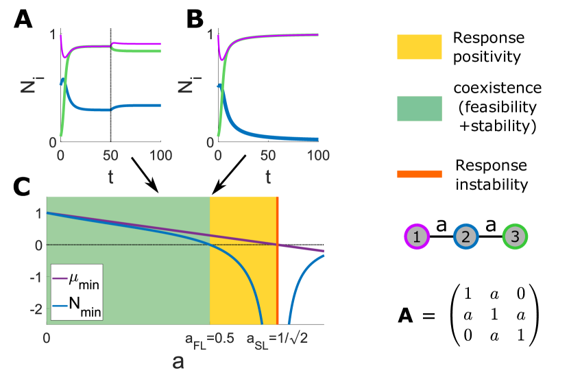
Figure 1: Feasibility, response stability, and an example for why feasibility breaks first. Behavior of a three species community. The species interact with interaction strength $a$ according to the interaction matrix $\mathbf{A}$, as shown in the diagram above $\mathbf{A}$. (A-B) The species abundances as a function of time for two values of $a$, and with arbitrarily chosen initial conditions. Each curve represents a different species, with the colors matching the species in the interaction diagram. (A) At $a=0.4$, the three-species community relaxes to an equilibrium at time $t\leq 50$. The equilibrium is feasible, that is, abundance values are positive. The equilibrium is also response-stable: At time $t=50$ a small change to the carrying capacities is applied to the system to test this, and produces only proportionally small changes in the equilibrium values. Varying interaction strengths $a$, these two conditions are satisfied for all $0<a<1/2$. (B) At $a=1/2$, one species reaches zero abundance, so species no longer coexist due to breaking of feasibility, while response stability is maintained. (C) The smallest abundance $N_{\text{min}}$, and the smallest eigenvalue of the interaction matrix $\mu_{\text{min}}$, as a function of $a$. $\mu_{\text{min}}$ acts as a measure of response stability: when it reaches zero at $a=a_{\text{SL}}=1/\sqrt{2}\approx 0.71$, perturbations can cause diverging changes in abundances. But we show that this also means that the abundances themselves diverge at $a=a_{\text{SL}}$, and in particular, $N_{\text{min}}\to-\infty$ there. This provides a mechanism for the earlier breaking of feasibility, as $N_{\text{min}}$ must indeed cross zero already at $a<a_{\text{SL}}$.

Here we take a different approach. We consider the space of possible interaction strengths and consider the region where all species of the system coexist. In this region, the conditions that must be satisfied are feasibility and Lyapunov stability (meaning that variables return to equilibrium if initiated close to it). We also consider another type of stability, response stability, meaning that small changes to carrying capacities (press perturbations [18]) only produce proportionally small changes in the equilibrium abundance values. See an example in Fig. 1(A-B). Focusing on systems with symmetric competitive interactions, we show that at the boundaries of the coexistence region it is generically feasibility that breaks first. By “generically” we mean that this is true everywhere except at special isolated points on the boundary (or more generally subspaces of lower dimension). In this sense feasibility is a more restrictive condition than stability. We proved part of this result as a lemma in a previous paper [19]. Our method is applicable to any number of species, not just ones with asymptotically many species, in contrast to other approaches discussed above. There might be additional interesting phenomena in the asymptotic limit of many species besides those considered here.

The breaking of feasibility before response stability can be understood by the following reasoning: when varying system parameters, as an instability is approached it generically induces large variations in species abundances. This in turn leads to extinctions before the instability is reached, thus breaking feasibility first, see example in Fig. 1(C). In this example, interactions are changed by increasing a single parameter $a$. The range of coexistence ends as the smallest species abundance crosses zero at a value $a=a_{\text{FL}}$, implying loss of feasibility. This can be related to the fact that the smallest eigenvalue of the interaction matrix reaches zero at some larger value $a_{\text{SL}}$, which we will show is associated with loss of stability. This causes some abundances to diverge towards $-\infty$ at this point, and indeed cross abundance zero before it. We will return to this example and explain it in more detail after defining all terms in our model. This understanding highlights the close links between stability and feasibility, and the necessity of studying them together.

An important consequence of our results is on the set of equilibria in ecological systems in the presence of migration, where systems may admit multiple equilibria in which some species are extinct. We show that as interaction strengths are changed continuously, coexistence is lost by the abundance of a single species going to zero, and the new fixed point where this species is extinct is unique. As parameters are further changed, multiple equilibria may then appear.

For mutualistic symmetric interactions, we show that at the boundary of the coexistence region feasibility and response stability break together. In the Lotka-Volterra model that we use, abundances diverge when crossing this boundary, indicating that this model cannot be used in this parameter regime. For systems that have a mixture of competitive and mutualistic interactions, either of the behaviors above is possible, with feasibility breaking with or before response stability. In all symmetric cases, the third possibility, where response stability breaks before feasibility, will require a special, fine-tuned combination of parameters. Finally, we extend our results to the case of asymmetric interactions, and discuss when the results above still apply.

The paper is structured as follows. We start by introducing the Lotka-Volterra model and the two definitions of stability. We then turn to our main claim: that for competitive symmetric interactions, feasibility generically breaks before response stability. We first use the single parameter example in Fig. 1 to demonstrate the basic mechanism behind this behavior and then prove it for a general case. We also discuss the behavior when there are some mutualistic interactions. Next, we discuss implications of our results on the manner in which new fixed points are formed as interaction strengths change. Lastly, we discuss asymmetric interactions, and when our results also extend to this regime.

II The model and stability definitions

We will consider the dynamics of $S$ species described by the Lotka-Volterra (LV) equations, where the dynamics of the abundance $N_{i}$ of species $i$ is given by

$$\frac{dN_{i}}{dt}=N_{i}g_{i}\left(\vec{N}\right)=N_{i}\rho_{i}\left(K_{i}-\sum_{j}A_{ij}N_{j}\right)$$ (1)

Here $g_{i}\left(\vec{N}\right)$ is the growth rate of species $i$, that depends on the interaction strengths $A_{ij}$, the carrying capacities $K_{i}$ (the long-time abundance reached by the species when isolated) and the bare growth rates of the species, $r_{i}\equiv\rho_{i}K_{i}$ (the growth rate at small numbers when isolated). Here the intraspecific interactions are all $A_{ii}=1$. For the first part of the paper, we will take symmetric interactions, with $A_{ij}=A_{ji}$ for all $i,j$. Both carrying capacities and bare growth rates are taken to be positive, $K_{i},r_{i}>0$. The feasibility condition in this formulation is that for all $i$, $N_{i}^{*}>0$, and so the fixed-point abundances can be found immediately by setting $g_{i}\left(\vec{N}^{*}\right)=0$, which gives $\vec{N}^{*}=\mathbf{A}^{-1}\vec{K}$, which yields a unique fixed point that must also satisfy $N_{i}^{*}>0$ in order for feasibility to hold. In general, all possible fixed points are found by choosing a set of species with $N_{i}^{*}=0$, then finding the rest of the abundances using $\vec{N}^{*}=\mathbf{A}^{-1}\vec{K}$ with $\mathbf{A},\vec{K}$ reduced to the species with $N_{i}^{*}\neq 0$; therefore once the set is chosen the fixed point is unique. Here we will (except in section V) consider the fixed point under the assumption that all species coexist, even in regions where it becomes unrealistic, as the solution yields some $N_{i}^{*}<0$.

When a feasible solution exists, the system will be in equilibrium if it is also stable. The term “stability” has many meanings in ecology [20]. Consider first Lyapunov stability, which is stability of the dynamics under small deviations of the abundances $N_{i}$ around their fixed point values $N_{i}^{*}$. By linearizing Eq. 1 about $\vec{N}^{*}$, it is satisfied when the real parts of the eigenvalues of the matrix $\mathbf{D}(\vec{N}^{*})\mathbf{A}$ are positive, where $\mathbf{D}(\vec{N}^{*})$ is a diagonal matrix with the equilibrium abundances $\vec{N^{*}}$ along the diagonal. This matrix is called the community matrix [4], and is denoted in the following by $\mathbf{DA}$. Although Lyapunov stability is only relevant on feasible systems (as the dynamics cannot reach a fixed point that is not feasible), we can still formally refer to the properties of $\mathbf{DA}$ as defining Lyapunov stability in the entire range of interaction strengths. For symmetric interactions, within the feasibility region the condition for Lyapunov stability is equivalent to the interaction matrix $\mathbf{A}$ being positive definite, denoted by $\mathbf{A}>0$ [21, 22, 23]. Therefore it will be sufficient to consider the condition that $\mathbf{A}$ is positive definite (instead of referring to the properties of $\mathbf{DA}$) , which is more easily accessible as it does not require finding the abundances $N_{i}^{*}$.

This condition is related to a second type of stability, which we term response stability. Response stability requires that once a Lyapunov stable fixed point with abundances $\vec{N^{*}}$ is reached, a small perturbation in the carrying capacities $K_{i}$ (known as a press perturbation [18]) yields small changes in the abundances $\vec{N}^{*}$ of a newly found fixed point. Since $\partial N_{i}^{*}/\partial K_{j}=\left(\mathbf{A}^{-1}\right)_{ij}$, response stability requires that $\mathbf{A}$ be invertible [24]. Response instability, where $\mathbf{A}$ has a zero eigenvalue, will first occur at the edge of the region where $\mathbf{A}>0$, which we will call the “response positivity” region. Although the underlying experiment, where a perturbation is applied, can only be done if the system is feasible and Lyapunov stable, we will (similarly to the case of Lyapunov stability) formally use the terms response stable or positive to describe the properties of $\mathbf{A}$ for any values of $A_{ij}$, even where these conditions may not be satisfied..

In the following we will consider the possible behaviors in the space of the off-diagonal elements $A_{ij}$ of the interaction matrix, for given $K_{i}$ and $\rho_{i}$. As $\mathbf{A}$ is an $S\times S$ matrix and $A_{ii}=1$, this space is of dimension $d=S\left(S-1\right)$ if the matrix is asymmetric, and $d=S\left(S-1\right)/2$ if it is symmetric. It might be convenient to look at lower-dimensional cross sections which are linear hyperplanes in this space (for example, by taking constraints where some of the interactions are zero or some are equal to each other, etc.). We will discuss the behavior of feasibility and stability within these spaces of matrix components. We will first discuss the cases where the interaction matrices $\mathbf{A}$ are symmetric with all positive entries, and later discuss the effects that breaking these assumptions has on the results.

III Feasibility breaks before stability: the basic mechanism

To explain the basic mechanism in play, we consider an example, see Fig. 1. This is a competitive (all $A_{ij}\geq 0$) three-species model, with symmetric interactions, such that the pairs of species (1,2) and (2,3) interact with strength $a\geq 0$, while species 1 and 3 do not interact directly. The carrying capacities and growth rates in isolation are all taken to be one, $K_{1,2,3}=1,\rho_{1,2,3}=1$. In this simple system, one can find the minimal eigenvalue of $\mathbf{A}$, $\mu_{\min}=1-\sqrt{2}a$, and the abundances, $N_{1}^{*}=N_{3}^{*}=\left(1-a\right)/\left(1-2a^{2}\right)$, $N_{2}^{*}=\left(1-2a\right)/\left(1-2a^{2}\right)$. The system is feasible for $a<1/2$ and $a>1$. It is response positive for $a<1/\sqrt{2}$, and response stability breaks at $a=1/\sqrt{2}$ (see Fig. 1). Coexistence, which requires feasibility and that $\mathbf{A}$ be response positive, breaks along with feasibility at $a=1/2$.

Let us analyze this behavior. At $a=0$, the interaction matrix is just $\mathbf{A}=\mathbf{I}$, with $\mathbf{I}$ the identity matrix. Thus all $N_{i}^{*}=K_{i}=1$, since $\vec{N}^{*}=\mathbf{A}^{-1}\vec{K}=\vec{K}$, and the system is both feasible and stable. As $a$ is increased, the eigenvalue $\mu_{\min}$ decreases, hitting zero at $a_{\text{SL}}\equiv 1/\sqrt{2}$. How does this affect the abundances $N_{1,2,3}^{*}$? As $\mu_{\min}$ approaches zero, the entries of the inverse matrix $\mathbf{A}^{-1}$ grow in absolute value until they diverge at $a_{\text{SL}}$. Since $\vec{N}^{*}=\mathbf{A}^{-1}\vec{K}$, the values of $\vec{N}^{*}$ will also become very large in absolute value, either positive or negative (This is true for all but very special $\vec{K}$ vectors, see next section.). Indeed, the minimal abundance, which is $N_{2}^{*}$ for $a<a_{\text{SL}}$, diverges to $-\infty$ precisely at $a_{\text{SL}}$. This means that $N_{2}^{*}$ had to cross zero at some smaller interaction strength, $a<a_{\text{SL}}$, breaking feasibility first.

For $a<a_{\mathrm{SL}}$, the minimum eigenvalue of the community matrix $\mathbf{DA}$ is $\nu_{\min}=\left(1+2a^{2}-3a\right)/\left(1-2a^{2}\right)$. Thus, Lyapunov stability is lost along with feasibility at $a=1/2$. As we will show below, Lyapunov stability will indeed generically break along with feasibility. Loss of Lyapunov stability is characterized by a slowdown of the dynamics, which occurs here when at $a=1/2$ the abundance $N_{2}^{*}$ approaches zero as a power-law in time.

To explore the special cases where stability breaks before feasibility, we expand this simple example by allowing for the interaction between species $(1,2)$ to have a different strength than that between species $(2,3)$, which we denote as $a_{A}$ and $a_{B}$ respectively (see Fig. 2). As shown in Fig. 2, when starting in the coexisting region and changing $a_{A},a_{B}$ continuously, response stability breaks before feasibility only along trajectories crossing one of the points $(a_{A},a_{B})=(1,0),(0,1)$. The behavior in this case will be expanded upon below.

IV Feasibility generically breaks before response stability for symmetric competition

We now prove the main result in the general case: for symmetric matrices with non-negative entries (i.e., competitive interactions), coexistence is lost through loss of feasibility rather than response stability. We start with a system in the coexistence region, by for example taking $A_{ij}=0$ for all $i\neq j$, which has a stable fixed point with all $N_{i}=K_{i}$. We then change the interactions along some path in $A_{ij}$ space. We show that the feasibility condition is the first to break, unless the choice of the path is fine tuned (namely, goes through special points, see below).

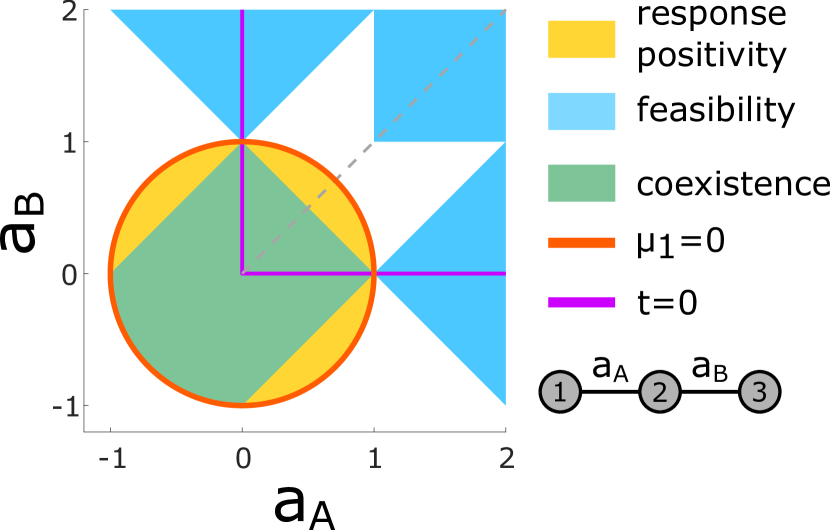
Figure 2: Geometry of stability and feasibility for symmetric interactions. The space of interaction strengths for a three-species system with two parameters, with the structure of interactions as shown. For all $i$, $K_{i}=1,\rho_{i}=1$. The dashed gray line indicates the parameter region shown in Fig. 1. Feasibility, response positivity ($\mathbf{A}>0$), and coexistence regions are shaded in blue, yellow and green respectively. Coexistence occurs in the intersection of the response positivity and feasibility regions. Response stability is lost on the manifold $\mu_{1}(\mathbf{A})=0$ (orange line). As can be seen, coexistence is lost by loss of feasibility (green region is surrounded by yellow region), except at two points; These points lie on the manifold $t(\mathbf{A})=0$ where there are no divergences in the abundances, allowing feasibility to be retained after loss of coexistence at the intersection of the two manifolds.

We will start by noting that for symmetric matrices, the region where the system is response positive with $\mathbf{A}>0$ is continuous and convex [25], and at its edge response stability is broken as $\mathbf{A}$ has a zero eigenvalue. However the feasibility region may be disconnected. Indeed for the example in Fig. 2(A-B), the response positive region is the convex unit disk; and the feasibility region in Fig. 1 is disconnected (recall that the green coexistence region is also a feasibility region).

Consider a trajectory in the $d$-dimensional space of interaction strengths, such that as we change $\{A_{ij}\}$ continuously, response stability is lost at a point $\mathbf{A}_{\text{SL}}$. As the matrix $\mathbf{A}$ is symmetric, it can be diagonalized with real eigenvalues $\left\{\mu_{i}\left(\mathbf{A}\right)\right\}_{i=1}^{S}$, and corresponding left- and right-eigenvectors $\vec{L}_{i}\left(\mathbf{A}\right),\vec{R}_{i}\left(\mathbf{A}\right)$, with $\vec{L}_{i}$ being row vectors and $\vec{R}_{i}$ column vectors (left- and right-eigenvectors are the same up to a transpose for symmetric matrices, but are separated here to allow a generalization to some asymmetric cases). Since response stability is lost at $\mathbf{A}_{\text{SL}}$, at least one eigenvalue becomes zero there, which WLOG we take to be $\mu_{1}\left(\mathbf{A}_{\text{SL}}\right)=0$. Assume for now that there is no degeneracy, so for all $i\neq 1$, $\mu_{i}\left(\mathbf{A}_{\text{SL}}\right)>0$.

The inverted matrix $\mathbf{A}^{-1}$ is written using the eigen-decomposition of $\mathbf{A}$ as

$$\mathbf{A}^{-1} =\sum_{i=1}^{S}\mu_{i}^{-1}\vec{R}_{i}\vec{L}_{i}$$ (2)

$$=\mu_{1}^{-1}\vec{R}_{1}\vec{L}_{1}+\sum_{i=2}^{S}\mu_{i}^{-1}\vec{R}_{i}\vec{L}_{i}$$

$$\equiv\mu_{1}^{-1}\vec{R}_{1}\vec{L}_{1}+\mathbf{W}_{1}$$

defining the matrix $\mathbf{W}_{1}\equiv\sum_{i=2}^{S}\mu_{i}^{-1}\vec{R}_{i}\vec{L}_{i}$. The abundances can be written as

$$\vec{N^{*}}=\mathbf{A}^{-1}\vec{K} =\frac{\vec{L_{1}}\vec{K}}{\mu_{1}}\vec{R}_{1}+\mathbf{W}_{1}\vec{K}$$ (3)

$$\equiv\frac{t_{1}\left(\mathbf{A}\right)}{\mu_{1}\left(\mathbf{A}\right)}\vec{R}_{1}+\vec{w}_{1}$$

with $t_{1}\left(\mathbf{A}\right)=\vec{L_{1}}\left(\mathbf{A}\right)\vec{K}$ and $\vec{w}_{1}\left(\mathbf{A}\right)=\mathbf{W}_{1}\left(\mathbf{A}\right)\vec{K}$.

In the neighborhood of $\mathbf{A}_{\text{SL}}$, all non-leading eigenvalues (with $i\geq 2$) have $\mu_{i}>0$. Therefore, the components of $\vec{w}_{1}$ are finite, and the abundances $\vec{N^{*}}$ are dominated by the first term in Eq. 3. Generically, $t_{1}\left(\mathbf{A}\right)\neq 0$, and so as the trajectory approaches $\mathbf{A}_{\text{SL}}$, $\mu_{1}\rightarrow 0$ and the abundances $N_{i}^{*}$ diverge. In a competitive system, at least one abundance $N_{i}^{*}$ must diverge towards $-\infty$: indeed, if for a given $i$, among the other species $j\neq i$ there are none that diverge to $N_{j}^{*}\to-\infty$, and at least one $j$ such that $N_{j}^{*}\to+\infty$, then $N_{i}^{*}=1-\sum_{j\neq i}A_{ij}N_{j}^{*}\rightarrow-\infty$. By continuity of the value of $N_{i}^{*}$ along the trajectory, it must then have $N_{i}^{*}=0$ at a point in the trajectory before $\mathbf{A}_{\text{SL}},$breaking feasibility. So in these cases, feasibility must break before response stability.

Stability can break without feasibility loss only in fine-tuned cases, where $t_{1}\left(\mathbf{A}_{\text{SL}}\right)=0$ so the abundances $N_{i}^{*}$ do not diverge. While the boundary of the response positivity region is a $d-1$ dimensional manifold, $\left\{\mathbf{A}|\min_{i}\Re\left[\mu_{i}\left(\mathbf{A}\right)\right]=0\right\}$, feasibility is retained only on trajectories that pass through a lower $d-2$ dimensional manifold that also satisfies $t_{i}\left(\mathbf{A}\right)=0$. More generally, if there is a degeneracy in $\mathbf{A}$ such that $k$ eigenvalues $\mu_{1},..,\mu_{k}$ are all zero for some region of $\left\{\mathbf{A}|\min_{i}\Re\left[\mu_{i}\left(\mathbf{A}\right)\right]=0\right\}$, feasibility can be retained if the $k$ conditions $t_{i}\left(\mathbf{A}_{\text{SL}}\right)=0$ for $i=1,..k,$ are satisfied. We also note that for $t_{1}\neq 0$, there may also be fine-tuned cases where only some, and not all, of the species abundances diverge, if by some symmetry some of the elements of $\vec{R}_{1}$ are zero.

In the example given in Fig. 2(A-B), the dimension of the space of interaction strengths is $d=2$. There, the minimal eigenvalue of $\mathbf{A}$ is $\mu_{\min}=1-\sqrt{a_{A}^{2}+a_{B}^{2}}$, so the response positivity region is the unit disk. The corresponding eigenvector is $\vec{L}_{1}\propto\left(a_{A},-\sqrt{a_{A}^{2}+a_{B}^{2}},a_{B}\right)$, so $t_{1}\left(\mathbf{A}\right)=0$ along the lines $a_{A}=0$ and $a_{B}=0$. Indeed, feasibility is retained only along trajectories that pass through the zero-dimensional points $\left(0,1\right),\left(1,0\right)$, where the lines $t=0$ intersect with the instability boundary.

We can also consider Lyapunov stability directly, by the condition $\mathbf{DA}>0$, rather than through demanding both feasibility and response positivity. One can easily see that a system is Lyapunov stable if it is feasible and response positive; and Lyapunov unstable if it is feasible but not response positive or vice-versa. Lyapunov stability will therefore always break with the first among response stability and feasibility to do so, and generically at the break of feasibility. To see this, we use the fact that for two symmetric matrices $\mathbf{M}_{1}$ and $\mathbf{M}_{2}$, if $\mathbf{M}_{1}$ is positive definite, the product $\mathbf{M}_{1}\mathbf{M}_{2}$ has real eigenvalues, with the same number of positive and negative eigenvalues as $\mathbf{M}_{2}$ [26]. As one of the response stability and feasibility conditions breaks, then respectively either $\mathbf{A}$ or $\mathbf{D}$ will have negative eigenvalues while the other matrix remains positive definite, so $\mathbf{DA}$ will have some negative eigenvalues and the system will not be Lyapunov stable.

When interactions are completely mutualistic, i.e., $A_{ij}<0$ for all $i\neq j$, we prove in appendix A that feasibility always breaks along with both types of stability. This occurs as abundances remain positive along the trajectory until reaching the instability at $\mathbf{A}_{\text{SL}}$, where all divergences are towards $+\infty$; but approaching $\mathbf{A}_{\text{SL}}$along the path in the opposite direction they all diverge towards $-\infty$. In cases where there is a mixture of both positive and negative interactions, either case is possible: without fine-tuning, feasibility will break either before response stability, if some of the abundances diverge towards $-\infty$ at $\mathbf{A}_{\text{SL}}$, or along with it if all abundance divergences are towards $+\infty$. Lyapunov stability will again break along with the first of the other two conditions to do so, by the same mechanism as in the all-competitive or all-mutualistic case, depending on whether feasibility breaks before or along with response stability respectively.

V New fixed points are formed upon exiting the coexistence region by a single species becoming extinct

Here we will discuss the consequences of our results for the possible fixed points of the system, in the case where there is a slow migration into the system from an external species pool. Here it will be interesting to investigate the multiple alternative equilibria of one system. As discussed below, when migration is small, species in each equilibrium are partitioned into “surviving” and “extinct”, the latter only supported at positive abundance by the migration. For symmetric interactions, we discuss three results: (1) In the coexistence region, the fully-coexisting fixed point is the only stable equilibrium of the system; (2) For competitive systems, just after coexistence is broken, there is a single fixed point with extinct species if this occurs due to feasibility loss, and multiple fixed points if it is due to stability loss; and (3) For mutualistic interactions, rather than reaching a fixed point, abundances grow to infinity with the dynamics outside the coexistence region and the Lotka-Volterra description breaks down. We will here discuss points (1) and (2), and prove point (3) in appendix A.

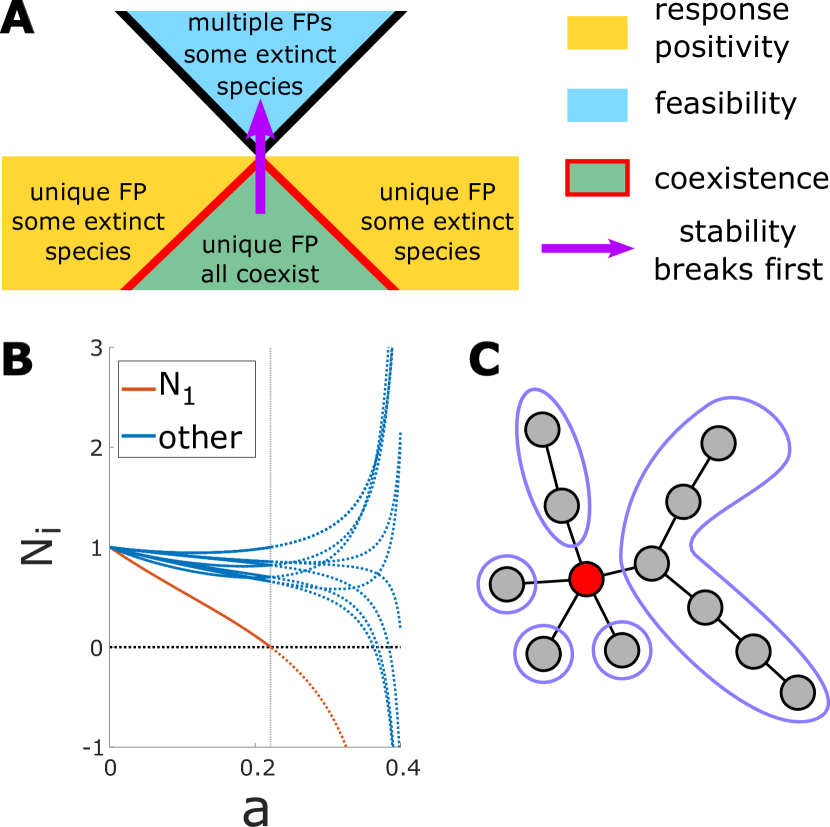
Figure 3: Fixed points in the presence of migration. (A) The behavior of fixed-points at the edge of the coexistence region in competitive systems. Feasibility, response positivity ($\mathbf{A}>0$) and coexistence regions are shaded in blue, yellow and green respectively. In the coexistence region, the only fixed point is the coexisting one. When coexistence breaks and the system remains response positive, there is a unique fixed point with extinct species. In the fine tuned cases where stability breaks before feasibility, there will be multiple fixed points with extinct species. (B-C) Example for a symmetric system where all interaction strengths are either $A_{ij}=0$ or $A_{ij}=a$. (B) The abundances as calculated by $\vec{N}^{*}=\mathbf{A}^{-1}\vec{K}$ as a function of $a$. The system coexists for $a=0$, and as $a$ is increased it loses feasibility at $a_{\text{FL}}\approx 0.22$ by the abundance of a single species, $N_{1}$, becoming zero. The calculation assumes all species coexist, so it becomes unrealistic for $a>a_{\text{FL}}$. (C) The structure of the equilibrium beyond $a_{\text{FL}}$. The species $N_{1}$ that goes extinct at the loss of feasibility is marked in red. In this case, when coexistence is lost, the interaction graphs breaks into several disconnected subgraphs, shown surrounded by purple lines.

Migration models a situation where individuals of different species can arrive from other locations in space that are not explicitly modeled. The Lotka-Volterra equations with constant migration read

$$\frac{dN_{i}}{dt}\equiv N_{i}g_{i}\left(\vec{N}\right)+\lambda_{i}$$ (4)

The effect of adding a migration term is that it allows an extinct species that has $g_{i}\left(\vec{N}\right)>0$ to return to the system. At the same time, we assume here that migration rates $\lambda_{i}$ are much smaller than the other parameters in the system, formally $\lambda_{i}\to 0^{+}$. Here we will consider fixed points where some species may be extinct with $N_{i}=0$. At a stable equilibrium, feasibility and Lyapunov stability must hold within the set of species that are not extinct. The calculation of the abundances $N_{i}^{*}$ and of the stability conditions within this set can be done by taking $\lambda_{i}\approx 0$. For extinct species migration entails an added condition, known as uninvadability, requiring that they all have negative growth rates.

For symmetric matrices, if long term abundances are bounded Eq. 4 always reaches a stable fixed point, albeit possibly one where some of the species are extinct ($N_{i}=0$). This is because the system admits a Lyapunov function whose maxima are the fixed points of the system [27]. For all positive interactions, abundances are bounded so the dynamics reach a fixed point with finite abundances. If some interactions are negative, abundances can grow until they diverge without reaching a fixed point.

Importantly, the Lyapunov function is convex if and only if the system is response positive [28]. Therefore, if the system is response positive the Lyapunov function cannot have multiple minima, so there is a unique stable fixed point. From here one immediately sees that in the coexistence region, where the system is response positive, the fixed point where all species coexist is the only equilibrium of the system [19]. From our main result, as parameters are changed, on approaching the edge of the coexistence region, the abundance of a single species generically goes continuously to zero while the system remains response positive. The system will then have a unique fixed point with only this species extinct, with abundances reached continuously from those at the coexisting fixed point.

An example application of this result, discussed in [19], is of systems with many species and sparse interactions, meaning that most $A_{ij}=0$. Such systems can be represented as sparse graphs, with vertices representing species and edges connecting interacting species. For large interaction strengths, at a fixed point the system breaks into many subsystems of persistent species (with $N_{i}>0$), separated by extinct species, and which can be considered as isolated systems. As interaction strengths are increased further, when any of these susbsystems stops coexisting it will be by a single species becoming extinct. Graphically, the subgraph of persistent species will further break into smaller graphs by removal of one extinct species, see example in Fig. 3B.

Without fine-tuning, a coexisting system cannot reach a phase with multiple fixed points by an infinitesimal change of parameters. This is because the occurrence of multiple fixed points requires stability to break down, which will occur only when varying the parameters further from the coexistence region, so that stability breaks as well. In the fine-tuned cases where stability breaks before feasibility, the system can have multiple fixed points, and in fact always has them just outside the coexistence region, as we prove in B. Further, the abundances at these new fixed points will not be reached continuously from those at the coexisting fixed point, as by definition they must be far from the unstable feasible fixed point. The geometry of the region near such a special point is shown in Fig. 3A, showing the fully-coexisting region, regions with partial coexistence (some species extinct), and multiple equilibria.

VI Asymmetric interactions

In this section we will discuss systems with asymmetric competitive interactions, i.e., where $A_{ij}\neq A_{ji}$ for some $i\neq j$, and all $A_{ij}\geq 0$. We start by discussing how the definitions we have used for response and Lyapunov stability are generalized to the asymmetric case. As in the symmetric case, we will see that generically feasibility breaks before response stability as a result of divergences in abundances. However in a difference from the symmetric case, coexistence can be constrained by Lyapunov stability alone, which would break before either feasibility or response stability without any fine tuning. We will discuss and show examples of cases where Lyapunov stability indeed breaks first, with no break in feasibility. On the other hand, we will show that there are classes of systems where the picture from the symmetric case holds, and feasibility is the factor constraining coexistence. We will then conclude with a short discussion of asymmetric mutualistic interactions.

An important difference between the symmetric and asymmetric case is that the matrices $\mathbf{A}$ and $\mathbf{DA}$ may have complex spectra, with eigenvalues that are complex conjugate pairs. For asymmetric interactions, Lyapunov stability requires that the real parts of all eigenvalues of $\mathbf{DA}$ be positive, causing abundances around the fixed point values $N_{i}^{*}$ to relax to the fixed point. In this case, even within the feasibility region, if the real parts of the eigenvalues of $\mathbf{A}$ are positive, this does not imply that the real parts of the $\mathbf{DA}$ eigenvalues are positive (although this does hold for certain large random matrices with probability one [8]). Therefore, unlike the symmetric case, in order to understand Lyapunov stability it is not enough to consider only the behavior of the matrix $\mathbf{A}$. Now consider how response stability (which again is defined at a Lyapunov-stable equilibrium) behaves in an asymmetric system. Response stability breaks when $\partial N_{i}^{*}/\partial K_{j}=\left(\mathbf{A}^{-1}\right)_{ij}$ diverges, which happens when $\mathbf{A}$ has an eigenvalue that is exactly zero. In particular, unlike for Lyapunov stability, response stability is not lost if a complex conjugate pair of $\mathbf{A}$ eigenvalues becomes purely imaginary as their real parts become zero.

As in the symmetric case, for all-positive interactions, the loss of response stability by an eigenvalue reaching zero will generically cause divergences in some abundances towards $-\infty$, so feasibility will break before response stability. Consider again changing the interaction strengths along a path in $A_{ij}$ space, as in Sec. IV. Again defining $\mathbf{A}_{\text{SL}}$ as the point in the path where the first eigenvalue of $\mathbf{A}$ becomes zero, from Eq. 3, if $t_{1}\left(\mathbf{A}\right)\neq 0$ there must be divergences in the abundances at the approach to $\mathbf{A}_{\text{SL}}$, meaning that feasibility breaks earlier. Note that if the eigenvalue is complex, and it is only its real part that becomes zero, response stability does not break and there would be no divergences in the abundances.

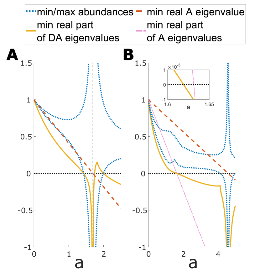
Figure 4: Asymmetric interactions. Matrices are of the form $\mathbf{A}=\mathbf{I}+a\mathbf{M}$, with values shown as a function of $a$. Shown are the maximal and minimal abundances, the minimum of the real parts of $\mathbf{DA}$ eigenvalues, and the smallest of the real-valued eigenvalues of $\mathbf{A}$. A gray vertical line marks the value of $a$ where the last becomes zero. As the curves represent minimal/maximal values, cusps appear when different values (say, the abundances of two different species) cross. The matrices $\mathbf{M}$ are given in appendix C. (A) The leading eigenvalue of $\mathbf{M}$ is real and the behavior is the same as for symmetric matrices. Abundances diverge as the eigenvalues of $\mathbf{A}$ approach zero, some of them towards $-\infty$; Lyapunov stability is broken along with feasibility (B) The leading eigenvalues of $\mathbf{M}$ are a complex conjugate pair. Lyapunov stability breaks first without a break in response stability, feasibility breaks later, and finally $\mathbf{A}$ becomes uninvertible. The minimum of the real parts of $\mathbf{A}$ eigenvalues is also shown in a thin dashed-dotted pink line, showing that there are no divergences when it hits zero. Inset: The same results, zoomed in to show that the minimum real parts of the eigenvalues of $\mathbf{A}$ and $\mathbf{DA}$ (pink and yellow lines, respectively) do not cross zero at the same value of $a$.

It is possible, however, that Lyapunov stability will break down before feasibility when interactions are asymmetric. Recalling the situation in the symmetric case, starting at the coexisting region and changing $A_{ij}$ continuously, either feasibility or response stability had to break down in order for Lyapunov stability to do so. As the eigenvalues of $\mathbf{DA}$ are real in the coexisting region, Lyapunov stability is lost by $\det(\mathbf{DA})=0$, which means that either $\det\mathbf{A}=0$, implying the loss of response stability, or $\det\mathbf{D}=0$, implying loss of feasibility. However if interactions are asymmetric this is not generally true, as Lyapunov stability can be lost by a pair of complex conjugate eigenvalues crossing the imaginary axis, so that $\det(\mathbf{DA})\neq 0$. There can therefore be cases where Lyapunov stability is lost before either feasibility or response stability, and so Lyapunov stability would be the condition limiting coexistence.

One example where Lyapunov stability is the more constraining condition without fine tuning, is cases where interaction strengths are increased indefinitely without loss of feasibility, a scenario which is impossible for symmetric interactions. This can occur along a trajectory in the $\left\{A_{ij}\right\}$ space where the smallest real eigenvalue of $\mathbf{A}$ is always positive, so $\mathbf{A}$ is always invertible and $\vec{N}^{*}=\mathbf{A}^{-1}\vec{K}$ never diverges. In some of these cases, abundances never reach zero for any finite-valued interaction strengths. On the other hand, Lyapunov stability always breaks for large enough interaction strengths, constraining coexistence. See Appendix C for further discussion and examples.

On the other hand, there are several interesting cases where, as in the symmetric case, feasibility is still the condition constraining coexistence:

1. The leading eigenvalue (meaning that with the smallest real part) of $\mathbf{DA}$ is real. This means that the smallest eigenvalue of $\mathbf{DA}$ has to cross zero in order to lose Lyapunov stability, and so the argument from the symmetric case applies. Our main result for symmetric interactions is therefore robust up to a finite asymmetric perturbation: consider a symmetric interaction matrix $\mathbf{A}_{\text{S}}$, to which asymmetry is added by taking $\mathbf{A}=\mathbf{A}_{\text{S}}+\epsilon\mathbf{A}_{\text{AS}}$, where $\mathbf{A}_{\text{AS}}$ is an asymmetric matrix and $\epsilon\in\mathbb{R}$. When changing $\epsilon$ continuously from zero, there will be some finite region where the leading eigenvalue of $\mathbf{DA}$ remains real, as the eigenvalues would change continuously with $\epsilon$ and the appearance of a complex conjugate pair of eigenvalues would require two eigenvalues to meet on the real axis.

2. The leading eigenvalue of $\mathbf{A}$ is real. Testing linear trajectories in $\left\{A_{ij}\right\}$ space that cross the origin, we find that losing Lyapunov stability before feasibility seems to be a rare occurrence in these cases (see appendix D), although this may change for different types of trajectories.

3. The interaction graph is tree-like (i.e., it has no loops). In this case, the interactions can be symmetrized by rescaling the abundances as $N_{i}\rightarrow n_{i}=N_{i}/\tilde{K}_{i}$ with some $\tilde{K}_{i}>0$ (so that the carrying capacity becomes $K_{i}/\tilde{K}_{i}$) [28]. The $\left\{N_{i}\right\}$ system is at a fixed point iff $\left\{n_{i}\right\}$ is at a fixed point, and their stability and feasibility are the same (as $n_{i}>0$ iff $N_{i}>0$). Therefore, the stability and feasibility regions of the $\left\{n_{i}\right\}$ system are linear transformations of the regions of the $\left\{N_{i}\right\}$ system whose geometry remains the same.

In Fig. 4 we show examples of possible behaviors for asymmetric interactions, using linear paths in $\left\{A_{ij}\right\}$ space: we take $\mathbf{A}=\mathbf{I}+a\mathbf{M}$, with $\mathbf{I}$ the identity matrix, $\mathbf{M}$ a constant matrix with zeros on the diagonal, and $a>0$ a real free parameter. The behaviors are not fine-tuned, and remain unchanged when adding random perturbations to $M_{ij}$, $i\neq j$, from a normal distribution $\mathcal{N}\left(0,10^{-4}\right)$. For the matrices $\mathbf{A},\mathbf{DA}$ the relevant value for the loss of response/Lyapunov stability are shown: for $\mathbf{A}$ the smallest eigenvalue that is real, and for $\mathbf{DA}$ the smallest of the real parts of the eigenvalues. In 4A, all eigenvalues of $\mathbf{A}$ are real and $\mathbf{DA}$ has a real leading eigenvalue in the range shown, so the resulting behavior is the same as for symmetric interactions where feasibility breaks first. The abundances diverge as the minimal eigenvalue of $\mathbf{A}$ reaches zero, and so before this happens feasibility is lost and the minimum real part of the $\mathbf{DA}$ eigenvalues becomes zero. In 4B, neither the leading eigenvalue of $\mathbf{A}$ nor of $\mathbf{DA}$ is real. Lyapunov stability breaks first, followed by feasibility, and lastly an eigenvalue of $\mathbf{A}$ becomes zero. At this point, the abundances (of the Lyapunov unstable fixed point) diverge. Note that there is no divergence in the abundances when the minimal real part of the $\mathbf{A}$ eigenvalues becomes zero.

We conclude this section with a short discussion of the case of asymmetric all-mutualistic interactions (all $A_{ij}\leq 0$). If the interaction matrix $\mathbf{A}$ is irreducible (i.e., the associated interaction graph is strongly connected), feasibility and response stability break together, see proof in appendix A. In addition, for all-mutualistic interactions, when the system is feasible the eigenvalues of $\mathbf{DA}$ have positive real parts if the eigenvalues of $\mathbf{A}$ have positive real parts [21, 22, 23]. Lyapunov stability will therefore hold at least up to the point where feasibility breaks. The condition of irreducibility is one which we can reasonably expect to hold in ecological systems. For example, it holds for cases where interactions are bidirectional, i.e. where $A_{ij}\neq 0\iff A_{ji}\neq 0$, as long as the system is not made up of separated components (in which case, each component can be considered as a separate system).

VII Discussion

We have considered, within the framework of the Lotka-Volterra equations, the relations between the feasibility and stability conditions required for species coexistence. For communities with symmetric competitive interactions, we find that as interaction strengths are changed continuously, coexistence is generically broken due to loss of feasibility. Stability can break before feasibility only in fine-tuned cases, and small changes in parameters will lead to feasibility breaking first. In this sense, feasibility is the condition restricting coexistence, so that stability alone is insufficient to understanding coexistence. While this was previously discussed for many-variable systems with randomly drawn interactions [8], we show this here for any finite number of species. Furthermore, feasibility and stability are closely interlinked: the loss of feasibility happens because abundances diverge when approaching response instability. This result is also robust to some finite asymmetric perturbations of the interactions.

Consider for comparison the approach of [13, 29, 14] to the stability-feasibility relation. In those works the two conditions are separated by taking the carrying capacities $K_{i}$ as free parameters. One can then first choose $a_{ij}$ such that the system is stable, then choose $K_{i}$ values that yield a feasible fixed point, which will give the feasibility region $\left\{\vec{K}|\vec{K}=\mathbf{A}^{-1}\vec{N},N_{i}>0\right\}$. This is complementary to our study, which looks at the effects of varying the interactions $\mathbf{A}$ rather than the carrying capacities $K_{i}$. To see the relation to the behavior we describe close to the loss of stability, note that at the loss of stability, the interaction matrix $\mathbf{A}$ becomes singular and the feasibility region of $\vec{K}$ collapses from an $S$-dimensional subspace to a lower-dimensional space, and sensitivity to changes in $\vec{K}$ is infinite (loss of structural stability). This relates to our result: retaining feasibility close to the loss of stability requires fine-tuning.

We also studied the implications of our results to the formation of multiple equilibria, in systems subject to external migration. Generically, when changing parameters away from the coexisting region, a new fixed point will appear by the abundance of a single species going continuously to zero. With a further change of the parameters, one may then cross into the multiple equilibrium regime.

Our work is focused on the case of a finite number of species. The present framework may still be useful in the limit of infinitely many species, but should be treated with care (for example, as the spectrum of the matrices becomes continuous). In particular, our framework can be useful in the study of large random systems in cases that are not covered by probabilistic arguments. Such a case is found in sparse systems, where for strong enough interactions, the surviving species may form multiple small interacting networks, that do not interact with each other [19].

Appendix A Mutualistic systems

Here we will prove a few claims from the main text on fully mutualistic interactions ($A_{ij}\leq 0$ for all $i\neq j$). All cases discussed here assume that the interaction matrix $\mathbf{A}$ is irreducible, a condition likely to hold for most ecological systems: it includes all systems where interactions are bidirectional (i.e., $A_{ij}\neq 0\iff A_{ji}\neq 0$), and specifically symmetric systems, that cannot be divided into non-interacting communities (in which case each system can be treated separately) [30]. First, we show that feasibility and response stability always break together. We then show that Lyapunov stability holds at least until feasibility and response stability break, and that for symmetric interactions it breaks simultaneously with them. Finally, we show that for the dynamics in the presence of migration, beyond the coexistence region the abundances all grow to infinity.

A.1 Feasibility and response stability break together

We will now prove that for mutualistic interactions where the interaction matrix is irreducible, feasibility and response stability break together. The proof is structured as follows:

1. From [31], in mutualistic systems (symmetric or otherwise) feasibility cannot break before response stability. To show that both break together, we need only show that there are species with negative abundances just outside the stability region.

2. To do this we first show that the leading eigenvalue of $\mathbf{A}$ is real and non-degenerate, and its corresponding eigenvector has all positive elements.

3. We use (2) to prove that on approaching $\mathbf{A}_{\text{SL}}$ from within the stable region, all abundances diverge towards $+\infty$, and on approaching it from the unstable region, all divergences are towards $-\infty$. Therefore all abundances are negative just outside the stability region and the conditions break together. See example in Fig. 5.

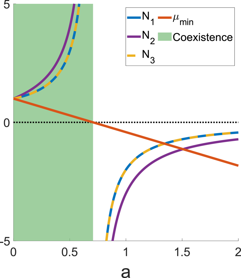
Figure 5: Divergences in abundances in mutualistic systems. Abundances and eigenvalues in a three species system, with species (1,2) and (2,3) interacting with $-a$, and taking $K_{i}=1,\rho_{i}=1$. Stability breaks as the minimum eigenvalue $\mu_{\text{min}}=1-\sqrt{2}a$ (red) becomes zero at $a_{\text{SL}}=1/\sqrt{2}$. All three abundances diverge towards $+\infty$ when approaching $a_{\text{SL}}$ from the coexistence region (green shading), and towards $-\infty$ when approaching $a_{\text{SL}}$ from outside the coexistence region.

To prove point (2), we use the Perron-Frobenius theorem for irreducible non-negative matrices [32], for the matrix $\mathbf{B}=-\left(\mathbf{A}-\mathbf{I}\right)$, where $\mathbf{I}$ is the identity matrix. $\mathbf{B}$ is non-negative: as all $A_{ii}=1$, it has zeros along the diagonal, and as interactions are mutualistic all other elements are non-negative. And if $\mathbf{A}$ is irreducible, then so is $\mathbf{B}$. The theorem states that the eigenvalue of $\mathbf{B}$ which has the maximal real part, called the Perron-Frobenius eigenvalue $\mu_{PF}$, is real, positive and non-degenerate. Further, its corresponding eigenvector has all positive components. The smallest eigenvalue of the matrix $\mathbf{A}$ is therefore $\mu_{1}=1-\mu_{PF}$, with the same corresponding eigenvector.

To prove (3), consider again the equation for the abundances from the main text,

$$\vec{N}=\left(t_{1}/\mu_{1}\right)\vec{R}_{1}+\vec{w}_{1}\,.$$ (5)

From (2), $\vec{L}_{1},\vec{R}_{1}$ have all positive components, and so also $t_{1}\left(\mathbf{A}\right)=\sum_{i}L_{1}^{i}K_{i}>0$ (recalling that all $K_{i}>0$). As instability is approached and $\mu_{1}\rightarrow 0^{+}$, the first term in Eq. 5 is strictly positive and diverges at the limit, with all other terms finite. Therefore as stability is lost, all abundances diverge to $N_{i}\rightarrow+\infty$. Approaching the same point from outside the stability region, $\mu_{1}\rightarrow 0^{-}$, and the abundances are still dominated by the term $\left(t_{1}/\mu_{1}\right)\vec{R}_{1}$. As the eigenvector components are still all positive and $\mu_{1}<0$, all abundances diverge to $-\infty$, so the system is unfeasible. Note that $t_{1}\left(\mathbf{A}\right)\neq 0$, so there can be no fine-tuned case where response stability breaks but feasibility does not.

A.2 Feasibility and Lyapunov stability break together for symmetric interactions

We will now move to investigate Lyapunov stability. First, as mentioned in the main text, in mutualistic systems Lyapunov stability and response stability are equivalent in the feasible region. Lyapunov stability therefore cannot break without a break in either feasibility or response stability. Specifically for symmetric systems, Lyapunov stability will break exactly at the loss of feasibility and response stability. To see this, consider a point in the trajectory just beyond the loss of feasibility. Here all abundances are very negative, so the matrix $-\mathbf{D}$ is positive definite. Recall the theorem used in the main text: for two symmetric matrices $\mathbf{M}_{1}$,$\mathbf{M}_{2}$, if $\mathbf{M}_{1}$ is positive definite then the product $\mathbf{M}_{1}\mathbf{M}_{2}$ has the same number of positive and negative eigenvalues as $\mathbf{M}_{2}$. Therefore, the matrix $-\mathbf{DA}$ has the same number of positive eigenvalues as $\mathbf{A}$. As just outside the stability region at least one eigenvalue of $\mathbf{A}$ must be positive (in the generic case, this would be all eigenvalues except one), $-\mathbf{DA}$ has a positive eigenvalue, and therefore $\mathbf{DA}$ has at least one negative eigenvalue and the system is not Lyapunov stable.

A.3 Dynamics in the presence of migration for symmetric interactions

Here we will show that outside the coexistence region abundances grow to infinity for any initial condition, and the Lotka-Volterra description breaks down. This is because there can be no stable and uninvadable fixed point with extinct species, since an extinct species $i$ would have a positive growth rate:

$$g_{i}\left(\vec{N}\right) =K_{i}-N_{i}-\sum_{j\neq i}A_{ij}N_{j}$$

$$=K_{i}+\sum_{j\neq i}\left|A_{ij}\right|N_{j}>0\,.$$

Therefore, outside the coexistence region the system has no feasible equilibrium nor one with extinct species. As for symmetric interactions the system has a Lyapunov function, it cannot reach a limit cycle or a chaotic state, and so the only possible dynamics is that some abundances keep growing to infinity.

Appendix B Scenario for generating multiple fixed points

Figure 6: Two species example of the formation of multiple fixed points in regions that are feasible and Lyapunov unstable. Trajectories of the LV equations in the phase space of the abundances $\left(N_{1},N_{2}\right)$ for $A_{12}=A_{21}=2$, and $\rho_{1,2}=1,K_{1,2}=1$. For these parameters the system is feasible and Lyapunov unstable. The two stable fixed points $\left(N_{1},N_{2}\right)=\left(0,1\right),\left(1,0\right)$, where one of the species is extinct, are marked with filled black circles. The unstable coexisting fixed point $\left(N_{1}^{*},N_{2}^{*}\right)=\left(1/3,1/3\right)$, is marked with an empty red circle. It has one stable direction, with the trajectories of the Lotka-Volterra dynamics that stably reach it marked in red. The unstable trajectories, starting at the unstable fixed point and reaching the stable ones, are marked in black. Other trajectories are shown in blue. No trajectory can cross the red line, and therefore there must be at least one stable fixed point on either side of it.

In this appendix we will prove the claim from the main text: for symmetric competitive interactions, in the fine tuned cases where Lyapunov stability is broken before feasibility, there will be multiple stable fixed points just outside the coexistence region. To see this, we will consider trajectories of the LV dynamics in the $S$-dimensional $\vec{N}$ space of the abundances. Note that here we are working in the space of the abundances $N_{i}$ for some given $\mathbf{A}$, rather than in $A_{ij}$ space considered in the rest of the paper. For each species, the dynamics are bounded from below by $N_{i}\geq 0$. At longer times they are also bounded from above by $K_{i}$, as the growth rate, $K_{i}-N_{i}-\sum_{j\neq i}A_{ij}N_{j}\leq K_{i}-N_{i}$, is negative when $N_{i}$ exceeds $K_{i}$.

As the system is still feasible, the fixed point where all species coexist is inside this bounded region, but is unstable. As we will show, the linear stability matrix $\mathbf{DA}$ has only a single negative eigenvalue, so in the vicinity of the fixed point there is a single unstable direction of the corresponding eigenvector. Therefore, there is an $S-1$ dimensional manifold of points that stably reach the coexisting fixed point. See example for two species in Fig. 6, where the stable manifold is a one dimensional line in the two-dimensional $\vec{N}$ space. As trajectories cannot cross each other, no trajectory of the LV dynamics can cross this manifold. The stable manifold therefore separates the bounded region into two parts, where dynamics with initial conditions in one region cannot reach the other one. As the system has a Lyapunov function, initial conditions in each of these two bounded regions must reach a stable fixed point, and so in each of them there must be at least one such fixed point. The importance of the condition that Lyapunov stability breaks before feasibility to this argument, is that this ensures that the coexisting fixed point is still feasible, so starting close to it is guaranteed to lead to fixed points with positive abundances.

We need now only prove our assumption, that just outside the coexistence region, $\mathbf{DA}$ indeed has exactly one negative eigenvalue. To prove this, we again use the fact that the eigenvalues of a product of two symmetric matrices, one of which is positive definite, have the same sign as the eigenvalues of the second matrix [26]. Excluding cases with extra symmetries where $\mathbf{A}$ has some degeneracy, response stability is lost as a single eigenvalue of $\mathbf{A}$ becomes negative. As feasibility is kept, however, all $N_{i}^{*}>0$ and the matrix $\mathbf{D}$ is positive definite. From here the linear stability matrix $\mathbf{DA}$, like the matrix $\mathbf{A}$, has a single negative eigenvalue.

Appendix C Possible behaviors for competitive asymmetric interactions

Here we provide additional explanations and examples of the behavior of competitive asymmetric interactions, demonstrating that the order in which feasibility, Lyapunov stability and response stability break can be the same as in the symmetric case or different from it. We expand on the scenario described in the main text, where interaction strengths are increased without causing divergences in the abundances. We also give the matrices used in examples in the main text. In all examples, we consider linear paths in $\left\{A_{ij}\right\}$ space: we take matrices of the form $\mathbf{A}=\mathbf{I}+a\mathbf{M}$, with $\mathbf{I}$ the identity matrix, $\mathbf{M}$ a constant non-negative matrix with zeros on the diagonal, and $a>0$ a real, positive number, and consider what happens as $a$ is increased.

First, the matrices used in Fig. 4 in the main text are

$$\mathbf{M}_{\text{A}} =\left(\begin{array}[]{ccc}0&0.4&0.4\\ 0.1&0&0.7\\ 0.1&0.5&0\end{array}\right)$$

$$\mathbf{M}_{\text{B}} =\left(\begin{array}[]{cccc}0&0.4&0.5&0.4\\ 0.6&0&0.2&0.9\\ 0.4&0.4&0&0.8\\ 0.5&0&0.8&0\end{array}\right)$$

with matrix $\mathbf{M}_{\text{X}}$ the matrix used in subfigure X. For $\mathbf{M}_{\text{A}}$ the leading eigenvalue of $\mathbf{DA}$ is real and therefore the behavior is the same as for symmetric interactions. This is not the case for $\mathbf{M}_{\text{B}}$, where Lyapunov stability breaks first, followed by feasibility, and lastly by response stability.

We will now turn to the following claim from Sec. VI of the main text: interaction strengths can in some cases be increased indefinitely, without producing divergences in the abundances. This occurs along paths where $\mathbf{A}$ is always invertible, so $\vec{N}^{*}=\mathbf{A}^{-1}\vec{K}$ never diverges. Feasibility may still be lost by an abundance crossing zero (although it is not forced to do so because of a divergence), but there are trajectories in the $A_{ij}$ space along which feasibility is not lost for any finite interaction strength. On the other hand, Lyapunov stability always breaks for large enough interaction strengths, and so it will be the condition limiting coexistence in the cases where feasibility never breaks. This behavior cannot occur for symmetric matrices, except in the fine-tuned cases where Lyapunov stability breaks first.

Consider again linear trajectories with $\mathbf{A}=\mathbf{I}+a\mathbf{M}$. Consider first a symmetric matrix $\mathbf{M}$. As $\text{tr}\mathbf{M}=0$ and the eigenvalues are all real, then some must be positive and some negative. Therefore, if $\mu_{\mathbf{M}}$ is the smallest eigenvalue of $\mathbf{M}$, it must be negative and response stability breaks at $a=-1/\mu_{\mathbf{M}}$. The region where a symmetric matrix is invertible is therefore bounded, and its boundary will be crossed along any trajectory when interactions are sufficiently increased. Without fine-tuning, this will cause divergences in the abundances. In contrast, if $\mathbf{M}$ is asymmetric, as it has complex eigenvalues it might have no real negative eigenvalues even though $\text{tr}\mathbf{M}=0$. So upon increasing $a$, response stability never breaks and there are no divergences in the abundances.

We will now show that Lyapunov stability always breaks for large enough $a$. Since $\mathbf{D}$ is diagonal, all $A_{ii}=1$, and the abundances are of the order $1/a$, $\text{tr}\mathbf{DA}=\sum_{i}D_{ii}A_{ii}=\sum_{i}N_{i}=O\left(1/a\right)$. On the other hand, as $\mathbf{A}$ is of order $a$, the off diagonal elements of $\mathbf{DA}$ are of order $1$. Therefore, the eigenvalues of $\mathbf{DA}$ are of order $1$, and so some of them must have negative real parts.

In Fig. 7 we show two examples of cases where there are no divergences in the abundances. In 7A, feasibility is lost for some positive $a$, and in 7B it is never lost. The matrices used are

$$\mathbf{M}_{\text{A}} =\left(\begin{array}[]{ccc}0&0.2&0.3\\ 0.9&0&0\\ 0.8&0.7&0\end{array}\right)$$

$$\mathbf{M}_{\text{B}} =\left(\begin{array}[]{ccc}0&0.9&0.2\\ 0.3&0&1\\ 0.7&0.6&0\end{array}\right)$$

The $a$-dependent abundances for $\mathbf{M}_{\text{B}}$ are given by $N_{i}^{*}\left(a\right)=\left(\mathbf{I}+a\mathbf{M}_{\text{B}}\right)^{-1}\vec{K}$ (for all $K_{i}=1$). No species ever has an abundance of zero, since $N_{i}\left(a\right)=0$ has no real solution for $a$; however $N_{i}^{*}$ tends to zero as $a\rightarrow\infty$. The behaviors are not fine-tuned, and remain unchanged when adding random perturbations to $M_{ij}$, $i\neq j$, from a normal distribution $\mathcal{N}\left(0,10^{-4}\right)$.

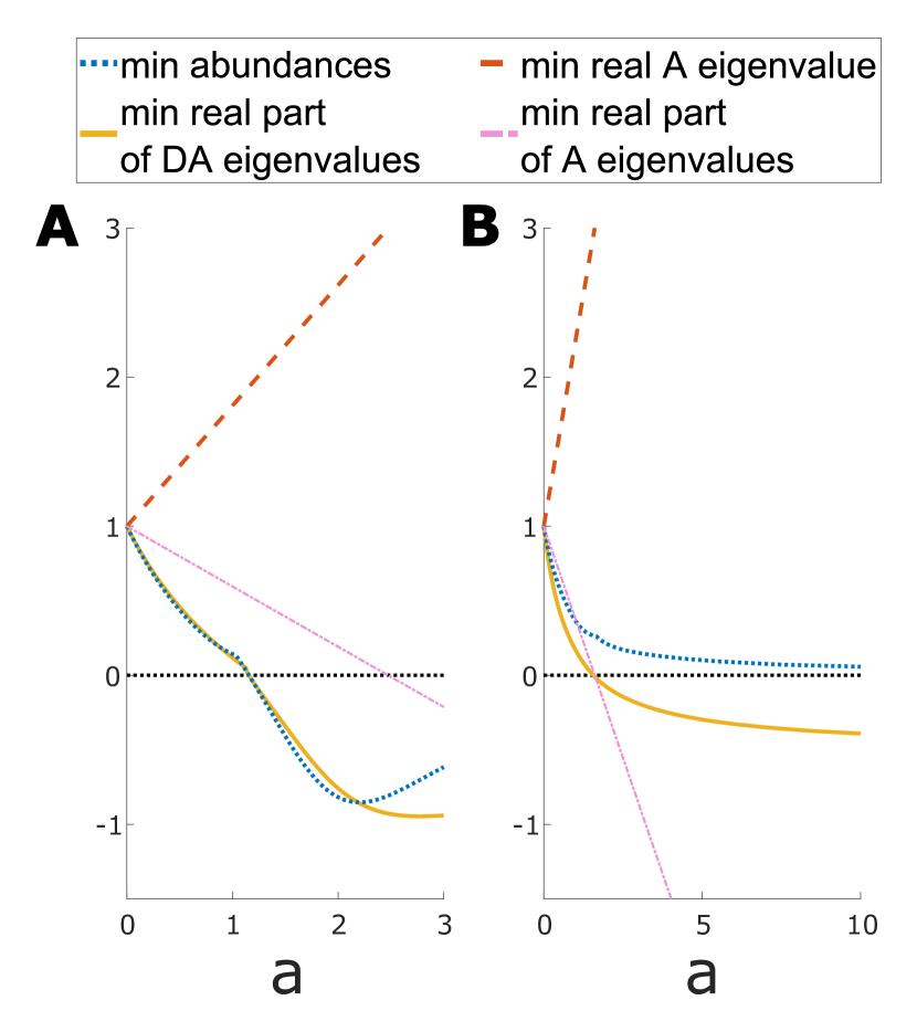
Figure 7: Asymmetric interactions with no divergences in the abundances. Matrices are of the form $\mathbf{A}=\mathbf{I}+a\mathbf{M}$, with values shown as a function of $a$. The minimal abundance is shown in a dotted blue line. The minimum of the real parts of $\mathbf{DA}$ eigenvalues is in a full yellow line. The dashed red line shows the smallest of the real valued eigenvalues of $\mathbf{A}$ and is linear with $a$. The minimum of the real parts of $\mathbf{A}$ eigenvalues is shown in a thin dashed-dotted pink line. In both cases, the smallest real eigenvalue of $\mathbf{M}$ is positive and so $\mathbf{A}$ is always invertible. As a result, the abundances do not diverge (A) feasibility and Lyapunov stability break together (B) Only Lyapunov stability breaks. The abundances are positive for any positive finite $a$.

Appendix D Lyapunov stability breaking before feasibility for asymmetric matrices with a real leading eigenvalue

Here consider competitive asymmetric matrices $\mathbf{A}$ with a leading real eigenvalue, and check whether Lyapunov stability breaks down before feasibility. Taking linear trajectories in $\left\{A_{ij}\right\}$ space that cross the origin, this seems to be a rare occurrence, although there may be other types of trajectories where this would be more common. We consider matrices of sizes $3\times 3$ and $4\times 4$ and of the form $\mathbf{A}=\mathbf{I}+a\mathbf{M}$, with $\mathbf{I}$ the identity matrix and $\mathbf{M}$ having zeros along the diagonal and off-diagonal elements taken from a uniform distribution over $\left[0,1\right]$. We randomly generate 10000 matrices $\mathbf{M}$ of each size, then see whether Lyapunov stability breaks before feasibility as $a$ is increased. For $3\times 3$ matrices, we find that for matrices $\mathbf{M}$ that have a real leading eigenvalue, this occurs with probability of about $0.36\%$, in contrast to probability of about $6.8\%$ for matrices where the leading eigenvalue is a complex conjugate pair. For $4\times 4$ matrices, for matrices $\mathbf{M}$ that have a real leading eigenvalue, this occurs with probability of about $0.43\%$, in contrast to probability of about $12.7\%$ for matrices where the leading eigenvalue is a complex conjugate pair.

References

- [1] Robert M. May and Angela R. McLean, editors. Theoretical Ecology: Principles and Applications. Oxford University Press, Oxford ; New York, 2007.
- [2] Alan Roberts. The stability of a feasible random ecosystem. Nature, 251(5476):607–608, October 1974.
- [3] Robert M. May. Will a large complex system be stable? Nature, 238(5364):413–414, August 1972.
- [4] R. M. May. Stability and complexity in model ecosystems. Monogr Popul Biol, 6:1–235, 1973.
- [5] Ian D. Rozdilsky and Lewi Stone. Complexity can enhance stability in competitive systems. Ecology Letters, 4(5):397–400, 2001.
- [6] Mike S. Fowler. Increasing community size and connectance can increase stability in competitive communities. Journal of Theoretical Biology, 258(2):179–188, May 2009.
- [7] Lewi Stone. The google matrix controls the stability of structured ecological and biological networks. Nature Communications, 7(1):12857, September 2016.
- [8] Lewi Stone. The feasibility and stability of large complex biological networks: A random matrix approach. Sci Rep, 8(1):8246, December 2018.
- [9] Guy Bunin. Ecological communities with lotka-volterra dynamics. Phys. Rev. E, 95(4):042414, April 2017.
- [10] Giulio Biroli, Guy Bunin, and Chiara Cammarota. Marginally stable equilibria in critical ecosystems. New J. Phys., 20(8):083051, August 2018.
- [11] Valentina Ros, Felix Roy, Giulio Biroli, Guy Bunin, and Ari M. Turner. Generalized Lotka-Volterra Equations with Random, Nonreciprocal Interactions: The Typical Number of Equilibria. Physical Review Letters, 130(25):257401, June 2023.
- [12] John H. Vandermeer. Interspecific competition: A new approach to the classical theory. Science, 188(4185):253–255, 1975.
- [13] Yuri Mikhailovich Svirezhev and Dmitrij Olegovič Logofet. Stability of Biological Communities. MIR Publishers, 1983.
- [14] Rudolf P. Rohr, Serguei Saavedra, and Jordi Bascompte. On the structural stability of mutualistic systems. Science, 345(6195):1253497, July 2014.
- [15] Serguei Saavedra, Rudolf P. Rohr, Jens M. Olesen, and Jordi Bascompte. Nested species interactions promote feasibility over stability during the assembly of a pollinator community. Ecology and Evolution, 6(4):997–1007, 2016.
- [16] Serguei Saavedra, Rudolf P. Rohr, Jordi Bascompte, Oscar Godoy, Nathan J. B. Kraft, and Jonathan M. Levine. A structural approach for understanding multispecies coexistence. Ecological Monographs, 87(3):470–486, 2017.
- [17] Chuliang Song, Rudolf P. Rohr, and Serguei Saavedra. A guideline to study the feasibility domain of multi-trophic and changing ecological communities. Journal of Theoretical Biology, 450:30–36, August 2018.
- [18] Edward A. Bender, Ted J. Case, and Michael E. Gilpin. Perturbation Experiments in Community Ecology: Theory and Practice. Ecology, 65(1):1–13, 1984.
- [19] Stav Marcus, Ari M. Turner, and Guy Bunin. Local and collective transitions in sparsely-interacting ecological communities. PLOS Computational Biology, 18(7):e1010274, July 2022.
- [20] Volker Grimm, Eric Schmidt, and Christian Wissel. On the application of stability concepts in ecology. Ecological Modelling, 63(1):143–161, September 1992.
- [21] G.W. Cross. Three types of matrix stability. Linear Algebra and its Applications, 20(3):253–263, June 1978.
- [22] Yasuhiro Takeuchi, Norihiko Adachi, and Hidekatsu Tokumaru. Global stability of ecosystems of the generalized volterra type. Mathematical Biosciences, 42(1):119–136, November 1978.
- [23] Abraham Berman and Daniel Hershkowitz. Matrix diagonal stability and its implications. SIAM. J. on Algebraic and Discrete Methods, 4(3):377–382, September 1983.
- [24] Mark Novak, Justin D. Yeakel, Andrew E. Noble, Daniel F. Doak, Mark Emmerson, James A. Estes, Ute Jacob, M. Timothy Tinker, and J. Timothy Wootton. Characterizing species interactions to understand press perturbations: What is the community matrix? Annual Review of Ecology, Evolution, and Systematics, 47(1):409–432, 2016.
- [25] Stephen P. Boyd and Lieven Vandenberghe. Convex Optimization. Cambridge University Press, Cambridge New York Melbourne New Delhi Singapore, version 29 edition, 2023.
- [26] Denis Serre. Matrices: Theory and Applications. Springer, New York, 2nd ed. 2010 edition edition, November 2010.
- [27] Robert MacArthur. Species packing and competitive equilibrium for many species. Theoretical Population Biology, 1(1):1–11, May 1970.
- [28] Yu.A. Pykh. Lyapunov functions for lotka-volterra systems: An overview and problems. IFAC Proceedings Volumes, 34(6):1549–1554, July 2001.
- [29] Dmitrij Olegovič Logofet. Matrices and Graphs: Stability Problems in Mathematical Ecology. CRC press, Boca Raton, 1993.
- [30] Feliks R. Gantmacher and Feliks R. Gantmacher. The Theory of Matrices. Vol. 2, volume 2. American Mathematical Soc, Providence, RI, reprinted edition, 2009.
- [31] Wei Su and Lei Guo. Interaction strength is key to persistence of complex mutualistic networks. Complex Systems, 25:157–168, June 2016.
- [32] Bas Lemmens and Roger D. Nussbaum. Nonlinear Perron-Frobenius Theory. Number 189 in Cambridge Tracts in Mathematics. Cambridge University Press, Cambridge ; New York, 2012.