Optimizing Layerwise Microservice Management in Heterogeneous Wireless Networks

Abstract

Small cells with edge computing are densely deployed in 5G mobile networks to provide high throughput communication and low-latency computation. The flexibility of edge computation is empowered by the deployment of lightweight container-based microservices. In this paper, we take the first step toward optimizing the microservice management in small-cell networks. The prominent feature is that each microservice consists of multiple image layers and different microservices may share some basic layers, thus bringing deep coupling in their placement and service provision. Our objective is to minimize the expected total latency of microservice requests under the storage, communication and computing constraints of the sparsely interconnected small cell nodes. We formulate a binary quadratic program (BQP) with the multi-dimensional strategy of the image layer placement, the access selection and the task assignment. The BQP problem is then transformed into an ILP problem, and is solved by use of a novel sphere-box alternating direction multipliers method (ADMM) with reasonable complexity $O(q^{4})$, where $q$ is the number of variables in the transformed problem. Trace-driven experiments show that the gap between our proposed algorithm and the optimal is reduced by 35$\%$ compared with benchmark algorithms.

1 Introduction

The complex services (e.g., mobile video , smart healthy care, real-time entertainment, augmented virtual reality) require lower latency and higher reliability for mobile network. Edge cloud has emerged as a promising platform complementary to central cloud systems by provisioning computing resources and mini data bases at the edge. By placing the cloud closer to the users, the mobile edge computing (MEC) network allows mobile users to acquire web service from nearby edge network. By doing so, MEC contributes to reduce the latency and mitigate the congestion in the backhual link [LYCT17]. Despite all the advantages, mobile edge computing is faced with some inherent challenges, e.g., various users’ demands, unbalanced workload, small coverage, and limited capacity [HNN⁺18]. To deal with it, small cells are introduced in 5G as a fundamental element of edge network. Benefiting from dense deployment, small cell nodes can operate in high frequencies, covering a range of 10 meters to 2 kilometers [HH18].

Under the requirement of improving users’ experience, container-based microservice is regarded as a promising pattern which organizes the traditional monolithic web application into a series of small web services [RN16, FFRR15, WLZ⁺18]. Each web service runs in a container with lower overhead. Cgroup and Kubernetes can effectively manage the containers on individual server or cluster while KubeEdge extend containerized orchestration capability to edge host. To provide certain web services, SCN needs to download the corresponding microservice image first. Microservice image is organized as layer structure and each layer provides necessary data, file or compilation environment. According to the downloading record of the Docker Hub, the image size of the most popular microservices can vary from 109MB to 2045MB which poses a great challenge to the limited storage resources of edge nodes. A recent study[HSL⁺16] pointed out that 57 most popular microservices images have 19 common base layers. Taking microservices of Cassandra, JAVA, Python, and gcc as examples, their images all require one non-latest Linux distribution layer of Debian. Layer sharing means that only one replica of common layer should be stored by SCN. According to Docker, microservice images can be pulled from repositories and stored in SCNs by layers with required functionalities instead of downloading the whole image.

Recently a great number of papers have investigated on microservice deployment strategies. [LAMC19, SJMW19] do not pay attention to the characteristics of microservices themselves, and only regard microservice containers as lightweight virtual machine. Without fully exploring the characteristics of microservices, the deployment strategies proposed by these papers often fail to make full use of the capacity of SCNs which results in a big gap between their solutions and optimal solution. Gu et al.[GZH⁺21b, GZH⁺21a] explored the layer structure and designed strategies to maximize the throughput. But in their model, they assume that if a microservice is requested then its image must be deployed in one and only in one server. After studying the real data, we find that the request frequency of microservices follows the long-tail distribution, that is, a small number of microservice requests occupy the majority of user requests while a large number of microservices are rarely requested. Therefore, deploying every requested microservices will contribute little to the improvement of users’ experience but will pay great cost.

In this paper, we aim to minimize the global latency of users in the 5G dense edge network. Given the distribution of users and the type of their requested microservice, diverse SCNs storage capacity and computing capacity, and edge network topology (i.e., connection relationship between SCNs and bandwidth), we will jointly deal with four essential questions: (1)for each SCN, what microservices should be deployed? (2)for each SCN, what layers should be deployed? (3)for each user, which AP should be selected to connect? (4)for each user, which SCN or central cloud should his task be assigned to? We formulate the above problem as a BQP problem. Due to the strong mutual dependency between microservice deployment and task assignment, our optimization problem turns to be intractable. In particular, microservice deployment can influence task assignment. Likewise, if a task is assigned to a SCN, the SCN must download the corresponding microservice image to provide web service.

On the principle of divide and conquer, we decompose the problem into several simple sub-problems. By completely solving these sub-problems, our BQP problem can be transformed into an ILP problem. But the transformed ILP is still intractable which is proved to be NP-hard. To tackle it, we propose a novel algorithm which is composed of two subroutine. First, we propose sphere-box ADMM algorithm which combines replacement method and ADMM to solve the ILP problem. We replace the binary constraint of the ILP problem with sphere constraint and box constraint and adopt ADMM algorithm to optimize it. This step will output a continuous solution whose elements are all close to 0 or 1. Second, we design a problem-specific rounding algorithm to turn the continuous solution obtained by sphere-box ADMM into final integer solution. Our major contribution are summarized below:

$\bullet$ To our best knowledge, this is the first work consider both the layer structure of microservice image and 5G dense edge network, and investigate how to minimize the global latency by jointly dealing with microservice deployment, layer deployment, AP selection and task assignment. We formulate the problem into a BQP problem.

$\bullet$ We propose a novel decomposition method to handle the BQP problem. By completely solving the sub-problems, the intractable BQP problem is transformed to an equivalent ILP problem which is much simpler and can be solved effectively.

$\bullet$ We design sphere-box ADMM to optimize the ILP problem and get continuous solution whose element are all close to 0 or 1. Then we design a problem specific rounding policy to convert the continuous solution into final integer solution.

$\bullet$ We analyze the date of Alibaba’s 2021 cluster-trace to figure out the characteristics of microservice requests distribution. Then the analysis results are used for experiment simulation. Extensive experiments are performed to verify that our algorithm can obtain close-to-optimal solution.

The remainder of this paper is organized as follows. Section 2 describes the proposed novel network architecture and formulate our problem. In section 3 we decompose our problem and propose our algorithm. The data analysis of real data trace and performance evaluation results are reported in Section 4. Finally, conclusions are then drawn in Section 5.

2 System Model

In this section, we describe the architecture of heterogeneous wireless networks in support of layer-wise microservices. Then we formulate the joint microservice deployment, AP selection and task assignment as a BQP problem.

2.1 Heterogeneous Edge Network

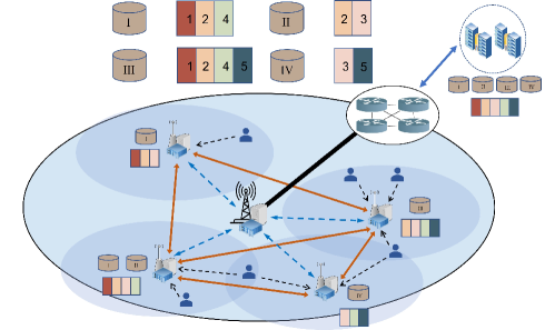
Figure 1: Small cell edge network with microservice provisioning

The architecture of our heterogeneous wireless networks is illustrated in Fig. 1 which conforms to European Telecommunication Standards Institute (ETSI) [KFF⁺18] and Federal Communications Commission (FCC) standards.

It consists of a macro cell node (MCN) and a number of densely deployed small cell nodes (SCNs). MCN directly connects to all the SCNs. Some SCNs are directly connected to each other through wired or fast wireless connection. Each user can connect to MCN or a SCN if he is within their overlapped transmission range. MCN and SCNs can connect to the central cloud through backhaul network. However, in practice, the bandwidth between the central cloud and the MCN is much higher than among SCNs [PIA⁺16]. Therefore we can consider that only MCN are connected to the central cloud. MCN can also be seen as a special SCN.

MCN and SCNs in support of microservices are equipped with computing and storage units with limited computing capability and storage space respectively. Hence, it cannot store all the microservice images locally and may not be able to handle multiple concurrent computations by itself. The central cloud has sufficient resource so we consider that the central cloud has deployed all the microservice images and can run infinite containers concurrently. MCN and SCNs also utilize a user plane function (UPF). With the help of UPF, the data traffic can be routed to other SCN. This enables collaboration between directly connected SCNs which means user requests web service from one SCN, but the service is actually performed by another SCN.

When a mobile user want to acquire web service from the edge cloud, he can connect to one of Sons which covers him to access the edge network. He can upload the data that he want to process and the type of microservice he wants to request. A SCN want to provide web service to user must corresponding microservice and has enough computing resource to start a container. Deploying a microservice means that the all the layers required by image have been stored. We call a SCN is available to a user when the SCN can provide service to the user [SHND19]. If the accessed SCN or one of its neighbor Sons is available, web service can be provide in the edge. Otherwise, the data will be offloaded to the central cloud and web service is provided by the cloud [PIST16].

2.2 Model Description

We consider an edge computing of a set $\mathcal{N}=\{1,\ldots,n,\ldots,N+1\}$ of SCNs. Among them, the index $N+1$ denotes MCN. For SCN-$n$, $S_{n}$, $C_{n}$ and $P_{n}$ to denote its storage capacity, computing capacity and location, respectively. They can be rewritten as the vectors $\mathbf{S}$, $\mathbf{C}$. For the connection relationship between the SCNs, we use a 0-1 matrix $\mathit{G}$ to depict the topology. For $n\neq m,\forall n,m\in\mathcal{N}$, $\mathit{G}_{n,m}$ is 1 which means that SCN-$n$ and SCN-$m$ are directly connected. Otherwise, SCN-$n$ and SCN-$m$ are not directly connected. Without loss of generality, we make all the elements in $G$’s diagonal be 1. If SCN-$n$ and SCN-$m$ are connected, the bandwidth between them are denoted as $B_{n,m}$. For the consistency of expression, we use $B_{N+1,N+2}$ to denote the backhaul bandwidth between MCN and the central cloud.

We use set $\mathcal{I}=\{1,\ldots,i,\ldots,I\}$ to denote all the microservices. We simply write the $i$th microservice as MS-i. Each microservice image is composed of some sharable layers and non-sharable layers. We denote the set of all layers existing in $\mathcal{I}$ as set $\mathcal{L}=\{1,\ldots,l,\ldots,L\}$. The storage space occupied by layer-$l$ is $K_{l}$. We use $H_{i,l}\in\{0,1\}$, $\forall i\in\mathcal{I}$, $\forall l\in\mathcal{L}$ to indicate whether layer-$l$ is required by MS-$i$ or not. To satisfy the service level agreement (SLA), when the mobile edge nodes provides service to mobile user, it must allocate some amount of computing resource to the container. Different micorservices require different amounts of computing resource. For MS-$i$, we let $F_{i}$ denote the required computation resource.

We consider the set of all users as $\mathcal{U}=\{1,\ldots,u,\ldots,U\}$. We simply write the $u$th user as MU-$u$. $Q_{u}$ presents his location. We let $M_{u}\in\mathcal{I}$, $R_{u}$ and $p_{u}$ denote the type of microservice requested by MU-$u$, the size of data to be processed and transmitting power of his end device, respectively. We use $W_{u,n}$ to denote the bandwidth between MU-$u$ and SCN-$n$.

The user’s latency consists of three parts: latency of uploading data, latency of computing and latency of returning result. Considering the computation time only relates to the size of data and the type of microservice. The size of calculation results is much smaller than the size of data which can be ignored [LHL⁺21]. We actually optimize the latency of data uploading.

3 Problem Formulation And Transformation

We will describe the decisions, constraints and objective function involved in our problem in detail.

3.1 Decision Variables

3.1.1 Microservice deployment

We define $\bm{x}\overset{\text{def}}{=}[\bm{x}_{1},\ldots,\bm{x}_{n},\ldots,\bm{x}_{N+1}]^{\mathrm{T}}$, where $\bm{x}_{n}\overset{\text{def}}{=}[x_{n,1},\ldots,x_{n,i},\ldots,x_{n,I}]^{\mathrm{T}}$ and $x_{n,i}\in\{0,1\}$, as the zero-one microservice deployment decision vector. The decision variable $x_{n,i}$ is an indicator variable defined as below:

$$x_{n,i}=\begin{cases}1,&\text{if MS-$i$ is deployed at SCN-$n$,}\\ 0,&\text{otherwise.}\end{cases}$$

3.1.2 Layer Deployment

We define $\bm{y}\overset{\text{def}}{=}[\bm{y}_{1},\ldots,\bm{y}_{n},\ldots,\bm{y}_{N+1}]^{\mathrm{T}}$, where $\bm{y}_{n}\overset{\text{def}}{=}[y_{n,1},\ldots,y_{n,l},\ldots,y_{n,L}]^{\mathrm{T}}$, as the zero-one layer deployment decision vector. The decision variable $y_{n,l}$ is an indicator variable defined as below:

$$y_{n,l}=\begin{cases}1,&\text{if layer-$l$ is deployed at SCN-$n$,}\\ 0,&\text{otherwise.}\end{cases}$$

3.1.3 AP Selection

We define $\bm{z}\overset{\text{def}}{=}[\bm{z}_{1},\ldots,\mathbf{z}_{u},\ldots,\mathbf{z}_{U}]^{\top}$, where $\bm{z}_{u}\overset{\text{def}}{=}[z_{u,1},\ldots,z_{u,n},\ldots,z_{u,N+1}]^{\top}$ and $z_{u,n}\in\{0,1\}$, as the zero-one AP selection vector. The decision variable $z_{u,n}$ is an indicator variable defined as below:

$$z_{u,n}=\begin{cases}1,&\text{if MU-$u$ connects to SCN-$n$,}\\ 0,&\text{otherwise.}\end{cases}$$

Each mobile user is capable of offloading his time-consuming and computation-intensive task to the SCNs or MCN through wireless channel. If MU-$u$ locates at the intersection of multiple SCNs’ coverage, then he can select one of them to access. We define indicator $\vartheta_{u,n}$ as below:

$$\vartheta_{u,n}=\begin{cases}1,&\text{if MU-$u$ is covered by SCN-$n$,}\\ 0,&\text{otherwise.}\end{cases}$$

3.1.4 Task Assignment

For the ease of expression, we use index $N+2$ to denote the central cloud.

We define $\bm{w}\overset{\text{def}}{=}[\bm{w}_{1},\ldots,\bm{w}_{u},\ldots,\bm{w}_{U}]^{\top}$, where $\bm{w}_{u}\overset{\text{def}}{=}[w_{u,1},\ldots,w_{u,m},\ldots,w_{U,N+2}]^{\top}$, as the zero-one task assignment decision vector. The decision variable $w_{u,n}$ is an indicator variable defined as below:

$$w_{u,m}=\begin{cases}1,&\text{if the task of MU-$u$ is assigned to SCN-$m$,}\\ 0,&\text{otherwise.}\end{cases}$$

For the sake of expression convenience, we add the $(N+2)$th column to the topology matrix $\mathit{G}$ which indicates whether a SCN can offload data to the central cloud or not. The elements in the new column are all 1.

3.1.5 Latency Description

We use $E_{u,n}$ to denote the bandwidth of wireless channel between MU-$u$ and one of accessible SCN-$n$.

Case1: task is assigned to accessed SCN. MU-$u$ uploads his request and data to SCN-$n$ and SCN-$n$ performs the computing task. The latency of MU-$u$ is only the latency of wireless communication between mobile device and access point:

$$t_{u,n,n}=\frac{R_{u}}{E_{u,n}}.$$

Case2: task is assigned to a neighbor SCN. MU-$u$ connects to SCN-$n$ to access the network and task is performed by its neighbor SCN-$m$. Therefore, we have the latency:

$$t_{u,n,m}=R_{u}(\frac{1}{E_{u,n}}+\frac{1}{B_{n,m}}).$$

Case3: task is assigned to the central cloud. In this case, the task of MU-$u$ is assigned to the central cloud.

If MU-$u$ accessed SCN-$n$, $n\in\mathcal{N}\setminus\{N+1\}$, his request and data must be routed to the MCN first and then can be offloaded to the central cloud. Therefore, the latency is:

$$t_{u,n,N+2}=R_{u}(\frac{1}{E_{u,n}}+\frac{1}{B_{n,N+1}}+\frac{1}{B_{N+1,N+2}}).$$

If MU-$u$ accesses MCN, his request can be offloaded to the central cloud straightforward. Therefore, the latency is:

$$t_{u,N+1,N+2}=R_{u}(\frac{1}{E_{u,n}}+\frac{1}{B_{N+1,N+2}}).$$

In convenience of expression, we define $t_{u,n,m}=O,\forall u\in\mathcal{U},\forall n\in\mathcal{N},\forall m\in\mathcal{N}\cup\{N+2\}$ where the $O$ is a large enough positive number when the situation where MU-$u$ can not access SCN-$n$ or task can not be assigned to SCN-$m$.

Considering for a user, the above mentioned three cases are complementary relationship, the latency of MU-$u$ can be expressed as the sum of the above expressions.

$$t_{u}=\sum_{n=1}^{N+1}\sum_{m=1}^{N+2}t_{u,n,m}z_{u,n}w_{u,m}$$

3.2 Problem Formulation

To minimize the global latency of all users, we can formulate our optimization problem into following form:

$$(\mathcal{P}_{1}) \min_{\mathbf{x},\mathbf{y},\mathbf{z},\mathbf{w}}\sum_{u=1}^{U}\sum_{n=1}^{N+1}\sum_{m=1}^{N+2}t_{u,n,m}z_{u,n}w_{u,m}$$ (1)

$$\text{s.t.: }\sum_{l=1}^{L}{y}_{n,l}K_{l}\leq S_{n},\forall n\in\mathcal{N},$$ (2)

$$y_{n,l}\geq H_{i,l}x_{n,i},\forall n\in\mathcal{N},\forall i\in\mathcal{I},\forall l\in\mathcal{L},$$ (3)

$$\sum_{n=1}^{N+1}\vartheta_{u,n}z_{u,n}=1,\forall u\in\mathcal{U},$$ (4)

$$\sum_{n=1}^{N+1}z_{u,n}=1,\forall u\in\mathcal{U},$$ (5)

$$\sum_{n=1}^{N+2}w_{u,n}=1,\forall u=1,2,\ldots,U,$$ (6)

$$w_{u,n}\leq x_{n,M_{u}},\forall u\in\mathcal{U},\forall n\in\mathcal{N},$$ (7)

$$\sum_{u=1}^{U}F_{M_{u}}w_{u,m}\leq C_{m},\forall m\in\mathcal{N},$$ (8)

$$\sum_{n=1}^{N+1}\sum_{m=1}^{N+2}\mathit{G}_{n,m}z_{u,n}w_{u,m}=1,\forall u\in\mathcal{U},$$ (9)

$$x_{n,m},y_{nl},z_{u,n},w_{u,m}\in\{0,1\},$$

$$\forall i\in\mathcal{I},\forall l\in\mathcal{L},,\forall u\in\mathcal{U},$$

$$\forall n\in\mathcal{N},\forall m\in\mathcal{N}\cup\{N+2\}.$$

Constraint (2) ensures that for each SCN, the layers deployed at it will not exceed its storage capacity. (3) indicates that when deploying a microservice, all the layers required by it need to be deployed first. Constraints (4) and (5) guarantee that a user will connect to one of his accessible SCNs. Constraint (6) ensures that a user’s task will be assigned to a SCN or to the central cloud. Constraint (7) indicates that when the task is assigned to a SCN, corresponding microservice need to be deployed first. In constraint (8), the total computing resource consumed by all tasks assigned to SCN-$m$ cannot exceed its capacity $C_{m}$. Constraint (9) ensures that the relationship between AP selection and task assignment is one of the three cases in section 3.1.5.

It’s a BQP problem with binary variables. Its objective function (1) and constraints (9) are quadratic. Its extremely non-convex nature makes it difficult to be analyzed theoretically, and it cannot be solved efficiently by off-the-shelf optimization algorithm. It is computationally prohibited in large size case when either the number of mobile user or the number of microservice is large.

3.3 Problem Decomposition and Transformation

Given a set of binary solution $(\bm{x}^{\prime},\bm{w}^{\prime},\bm{z}^{\prime})$ satisfying the constraint (2),(3),(6),(7),(8), we consider the sub-problem about $\bm{z}$.

$$(\mathcal{SP}_{1}) \min_{\bm{z}}\sum_{u=1}^{U}\sum_{n=1}^{N+1}\sum_{m=1}^{N+2}t_{u,n,m}z_{u,n}w_{u,m}^{\prime}$$

s.t.: (4),(5),(9),

$$z_{u,n}\in\{0,1\},\forall u\in\mathcal{U},\forall n\in\mathcal{N}.$$

This sub-problem is an ILP problem where each user accesses an accessible SCN to minimize the global latency. Since different users’ decisions are not coupled, the global latency is minimized if and only if the latency of each user is minimized.

We use $\xi_{u,m}$ to denote the shortest upload latency from MU-$u$ to SCN-$m$.

$$\xi_{u,m}=\min\{t_{u,n,m}|n\in\mathcal{N}\},\forall m\in\mathcal{N}\cup\{N+2\}.$$

We define $\zeta_{u,m}\in\mathcal{N}$ to denote which SCN is selected to access when the latency achieves $\xi_{u,m}$. If there are multiple SCNs can achieve such latency, we randomly choose one from them.

So the optimal value of the sub-problem ($\mathcal{SP}_{1}$) is $\displaystyle\sum_{u=1}^{U}\displaystyle\sum_{m=1}^{N+2}\xi_{u,m}w_{u,m}^{\prime}$. The optimal solution about $\bm{z}$ can be presented as follow:

$$z_{u,n}=\begin{cases}1,&\text{if $w^{\prime}_{u,m}=1$ and $n=\zeta_{u,m}$,}\\ 0,&\text{otherwise.}\end{cases}$$ (10)

By solving $(\mathcal{SP}_{1})$ with respect to $\bm{z}$ completely, $(\mathcal{P}_{1})$ can be transformed to an ILP formulation about $\{\bm{x},\bm{y},\bm{w}\}$ as follows:

$$(\mathcal{P}_{2}) \min_{\bm{x},\bm{y},\bm{w}}\sum_{u=1}^{U}\sum_{m=1}^{N+2}\xi_{u,m}w_{u,m}$$

s.t.: (2),(3),(6),(7),(8),

$$x_{n,m},y_{nl},z_{u,n},w_{u,m}\in\{0,1\},$$

$$\forall i\in\mathcal{I},\forall l\in\mathcal{L},,\forall u\in\mathcal{U},$$

$$\forall n\in\mathcal{N},\forall m\in\mathcal{N}\cup\{N+2\}.$$

This problem is still difficult to solve because of the tight coupling between micorservice deployment and task assignment. In Lemma 1, we show that the optimization problem ($\mathcal{P}_{2}$) is an NP-hard problem. However, through decomposition and transformation, the problem is greatly simplified when compared to the original problem ($\mathcal{P}_{1}$), which is very important to design efficient algorithm to solve later.

Lemma 1. The transformed optimization problem $(\mathcal{P}_{2})$ is NP-hard.

Proof. Given a solution $\{\bm{x}^{\prime},\bm{y}^{\prime}\}$ satisfying the constraints (1)(2), we explore the sub-problem $(\mathcal{SP}_{2})$ with respect to the variables $\bm{w}$.

$$(\mathcal{SP}_{2})\min_{\bm{w}}\sum_{u=1}^{U}\sum_{m=1}^{N+2}\xi_{u,m}w_{u,m}$$

$$\sum_{u=1}^{U}F_{M_{u}}w_{u,N+2}\leq\sum_{u=1}^{U}F_{M_{u}}.$$ (11)

$$\text{s.t.:(5),(6),(7)}.$$

$$w_{u,m}\in\{0,1\},\forall u\in\mathcal{U},\forall m\in\mathcal{U}\cup\{N+2\}$$

We add an extra constraint(21), but it is satisfied naturally when the decision variables are binary. In $(\mathcal{SP}_{2})$, we can regard the central cloud as a SCN with computing capability $\sum_{u=1}^{U}F_{M_{u}}$.

We regard the tasks as U items which need to be assigned and regard the SCNs and the central cloud as $N+2$ bins. The budget of bin-$n$ is the computing capability of SCN-$n$. The computing resource required by MU-$u$ is the weight of the $u$th item. The latency of MU-$u$ is the cost of the $u$th item. Constraints (5) and (6) indicate that some items can only be assigned to limited bins. Constraints (7) and (21) indicate that them items placed in a bin can not exceed the bin’s budget. The objective function is to minimize the total cost. This is a General Assignment Problem(GAP), which is NP-hard[ÖBT10].

Since sub-problem $(\mathcal{SP}_{2})$ is NP-hard, the main problem $(\mathcal{P}_{2})$ is also NP-hard.

4 Algorithm

To address $(\mathcal{P}_{2})$, in this section, we introduce sphere-box ADMM and a well-designed rounding policy which can effectively solve the transformed problem.

4.1 Sphere-box ADMM

The difficulty of solving ($\mathcal{P}_{2}$) mainly comes from the discontinuity caused by its domain of definition. Handling discrete space well is the key to solve the problem. Since our problem is not submodular like min-cut, the performance of heuristic algorithms such as greedy algorithm is neither good nor guaranteed performance. Exact algorithms such as branch and bound, cutting planes are computationally prohibited because it is NP-hard. Linear relaxation performs badly while semi-definition relation achieve better performance at the cost of much higher memory and computation. Therefore, we use replacement method to handle the discrete domain.

4.1.1 Sphere-box Replacement

We consider a binary space with $q$ variables. $\mathbf{u}\in\{0,1\}^{q}$ which is a binary vector. Box space $S_{b}=[0,1]^{q}$ is a convex continuous space and sphere space $S_{p}=\{\mathbf{u}|\|\mathbf{u}-\frac{1}{2}\mathbf{1}_{q}\|_{2}^{2}=\frac{q}{4}\}$ is a non-convex continuous space. According to Lemma2, we can replace the binary constraints in problem $(\mathcal{P}_{2})$ with constraint that the variables are in both the box space and the sphere space.

Lemma 2. The binary set $\{0,1\}^{q}$ can be equivalently replaced by the intersection between as box $S_{b}$ and a sphere $S_{p}$, as follows:

$$\bm{u}\in\{0,1\}^{q}\iff\bm{u}\in[0,1]^{q}\cap\begin{Bmatrix}\bm{u}:\|\bm{u}-\frac{1}{2}\mathbf{1}_{q}\|_{2}^{2}=\frac{q}{4}\end{Bmatrix}$$

The detail proof can be seen in [WG18]

4.1.2 ADMM Iteration Step

We concatenate the decision variables $\bm{x},\bm{y},\bm{w}$ to form a variable vector $\bm{v}=[\bm{x},\bm{y},\bm{w}]^{\mathrm{T}}$. We directly replace the binary constraints with them in ($\mathcal{P}_{2}$). We introduce auxiliary variables $\bm{e}_{1}$ in box space $S_{b}=[0,1]^{q}$ and auxiliary variables $\bm{e}_{2}$ in sphere space $S_{p}=\{\bm{e}_{2}:|\|\bm{e}_{2}-\frac{1}{2}\bm{1}_{q}\|_{2}^{2}=\frac{q}{4}\}$, where $q=(N+1)M+(N+1)L+(N+2)M$.

Since ($\mathcal{P}_{2}$) is an ILP problem, we can use matrix and vector to rewrite it as compact form as follows:

$$(\mathcal{P}_{3}) \min_{\bm{v},\bm{e}_{1},\bm{e}_{2}}\mathbf{f}^{\top}\bm{v}$$

s.t.:$$\mathbf{A}_{1}\bm{v}=\mathbf{g}_{1}$$,

$$\mathbf{A}_{2}\bm{v}+\mathbf{h}=\mathbf{g}_{2},$$

$$\bm{v}=\bm{e}_{1}=\bm{e}_{2},$$

$$\text{ }\bm{e}_{1}\in S_{b},\text{ }\bm{e}_{2}\in S_{p},\mathbf{g}\in\mathbb{R}_{+}^{q}.$$

Where the specific definition of each matrix and vector in ($\mathcal{P}_{3}$) can be found in Appendix A. Therefore, our ADMM update step is based on the following augmented Lagrangian expression:

$$\mathcal{LA}= \mathbf{f}^{\top}\bm{v}+\bm{k}^{\top}_{1}(\bm{v}-\bm{e}_{1})+\bm{k}^{\top}_{2}(\bm{v}-\bm{e}_{2})+\bm{k}^{\top}_{3}(\mathbf{A}_{1}\bm{v}-\mathbf{g}_{1})$$ (12)

$$+\bm{k}^{\top}_{4}(\mathbf{A}_{2}\bm{v}+\mathbf{h}-\mathbf{g}_{2})$$

$$+\frac{\rho_{1}}{2}\|\bm{v}-\bm{e}_{1}\|^{2}_{2}+\frac{\rho_{2}}{2}\|\bm{v}-\bm{e}_{2}\|^{2}_{2}$$

$$+\frac{\rho_{3}}{2}\|\mathbf{A}_{1}\bm{v}-\mathbf{g}_{1}\|^{2}_{2}+\frac{\rho_{4}}{2}\|\mathbf{A}_{2}\bm{v}+\mathbf{h}-\mathbf{g}_{2}\|^{2}_{2}$$

Here, $\bm{k}_{1},\bm{k}_{2},\bm{k}_{3},\bm{k}_{4}$ indicate dual variables, while $\rho_{1},\rho_{2},\rho_{3},\rho_{4}$ are positive penalty parameters.

Input : ADMM parameters and $\bm{v}^{0}$, $\bm{k}_{1}^{0}$, $\bm{k}_{2}^{0}$, $\bm{k}_{3}^{0}$, $\bm{k}_{4}^{0}$.

Output : $[\bm{x}^{\dagger},\bm{y}^{\dagger},\bm{w}^{\dagger}]$

while not converged do

       update $(\bm{e}_{1}^{t+1},\bm{e}_{2}^{t+1},\bm{h}^{t+1})$ according to Eqs.(13)(14)(15)

       update $\bm{v}^{t+1}$ by solving Eqs.(16)

       update $(\bm{k}_{1}^{t+1},\bm{k}_{2}^{t+1},\bm{k}_{3}^{t+1},\bm{k}_{4}^{t+1})$ as shown in Eqs.(17)

      

return $[\bm{x}^{\dagger},\bm{y}^{\dagger},\bm{w}^{\dagger}]=\bm{v}^{t+1}$

Algorithm 1 sphere-box ADMM

Update $\bm{e}_{1}^{t+1}$. We need to solve a sub-problem with respect to $\bm{e}_{1}$ as follows:

$$(\mathcal{SP}_{3})\bm{e}_{1}^{t+1}=\arg\min_{\bm{e}_{1}\in S_{b}}\bm{k}_{1}^{\top}(\bm{v}^{t}-\bm{e}_{1})+\frac{\rho_{1}}{2}\|\bm{v}^{t}-\bm{e}_{1}\|_{2}^{2}.$$

This is a quadratic problem with box constraints. We relax the box constraint. The relaxed problem is a simple quadratic problem which can be solved by setting its gradient to zero. The optimal solution is $\bm{e}_{1}^{\ast}=\bm{v}^{t}+\frac{1}{\rho_{1}}(\bm{k}_{1}^{t})^{\top}$. Since the contour of the objective function has a spherical shape, the optimal solution of ($\mathcal{SP}_{3}$) is the point closest to $\bm{e}_{1}^{\ast}$ in $S_{b}$. Since each of the faces of $S_{b}$ is perpendicular to each other, the point can be found by projecting $\bm{e}_{1}^{\ast}$ vertically onto each dimension and limit the coordinates to between 0 and 1. This projection process can be expressed in the following mathematical form:

$$\mathbf{P}_{S_{b}}(\bm{e}_{1}^{\ast})=\min(\mathbf{1},\max(\bm{e}_{1}^{\ast},\mathbf{0})).$$

Therefore, the optimal solution of $(\mathcal{SP}_{3})$ is:

$$\bm{e}_{1}^{t+1}=\mathbf{P}_{S_{b}}(\bm{v}^{t}+\frac{1}{\rho_{1}}(\bm{k}_{1}^{t})^{\top}).$$ (13)

Update $\bm{e}_{2}^{t+1}$. We need to solve a sub-problem with respect to $\bm{e}_{2}$ as follows:

$$(\mathcal{SP}_{4})\bm{e}_{2}^{t+1}=\arg\min_{\bm{e}_{2}\in S_{p}}\bm{k}_{2}^{\top}(\bm{v}^{t}-\bm{e}_{2})+\frac{\rho_{2}}{2}\|\bm{v}^{t}-\bm{e}_{2}\|_{2}^{2}.$$

This is a quadratic problem with a non-convex constraint $S_{p}$, which is a $(q-1)$-dimensional sphere centered at $\frac{1}{2}\mathbf{1}$ with radius $\frac{\sqrt{q}}{2}$. We relax the sphere constraints. The relaxed problem is a simple quadratic problem which can be solved by setting its gradient to zero. The optimal solution is $\bm{e}_{2}^{\ast}=\bm{v}^{t}+\frac{1}{\rho_{2}}(\bm{k}_{2}^{t})^{\top}$. Since the contour of the objective function has a spherical shape, the optimal solution of the original sub-problem is the point closest to $\bm{e}_{2}^{\ast}$ in the hollow sphere shell defined by $S_{p}$. The point is where the line between $\frac{1}{2}\mathbf{1}_{q}$ and $\bm{e}_{2}^{\ast}$ intersects the sphere $S_{p}$. This projection process can be expressed in the following mathematical form:

$$\mathbf{P}_{S_{p}}(\bm{e}_{2}^{\ast})=\frac{\sqrt{q}}{2}\frac{\bar{\bm{e}_{2}^{\ast}}}{\|\bar{\bm{e}_{2}^{\ast}}\|_{2}}+\frac{1}{2}\mathbf{1}.$$

where $\bar{\bm{e_{2}^{\ast}}}=\bm{e}_{2}^{\ast}-\mathbf{1}_{q}$. Therefore, $(\mathcal{SP}_{4})$ can be exactly solved by the following closed-form solution:

$$\bm{e}_{2}^{t+1}=\mathbf{P}_{S_{p}}(\bm{v}^{t}+\frac{1}{\rho_{2}}(\bm{k}_{2}^{t})^{\top}).$$ (14)

Update $\bm{h}^{t+1}$. Update the auxiliary variable $\bm{h}$ as the following method:

$$\bm{h}^{t+1}=\max(\mathbf{0},\mathbf{g}_{2}-\mathbf{\Upsilon}_{2}\bm{v}^{t}).$$ (15)

Update $\bm{v}^{t+1}$. We are required to solve three strongly convex quadratic problem without any constraints. We set the partial derivatives of the augmented lagrangian formula $\mathcal{L}$ with respect to the variables $\bm{v}$.

$$\begin{split}\frac{\partial\mathcal{LA}}{\partial\bm{v}}=&\mathbf{f}+\bm{k}_{1}+\bm{k}_{2}+\mathbf{A}_{1}^{\top}\bm{k}_{3}+\mathbf{A}_{2}^{\top}\bm{k}_{4}\\ &+\rho_{1}(\bm{v}-\bm{e}_{1})+\rho_{2}(\bm{v}-\bm{e}_{2})\\ &+\rho_{3}\mathbf{A}_{1}^{\top}(\mathbf{A}_{1}\bm{v}-\mathbf{g})+\rho_{4}\mathbf{A}_{2}^{\top}(\mathbf{A}_{2}\bm{v}+\mathbf{h}-\mathbf{g}_{2})\end{split}$$

We rearrange these above equation as the following positive-definite linear system for $\mathbf{v}$:

$$\begin{split}(\mathcal{SP}_{4})\Bigl{(}(&\rho_{1}+\rho_{2})\mathbf{I}+\rho_{3}\mathbf{A}_{1}^{\top}\mathbf{A}_{1}+\rho_{4}\mathbf{A}_{2}^{\top}\mathbf{A}_{2}\Bigr{)}\bm{v}^{t+1}\\ =&\rho_{1}\bm{e}_{1}^{t+1}+\rho_{2}\bm{e}_{2}^{t+1}+\rho_{3}\mathbf{A}_{1}^{\top}\mathbf{g}_{1}+\rho_{4}\mathbf{A}_{2}^{\top}(\mathbf{g}_{2}-\mathbf{h})\\ &-\mathbf{f}-\bm{k}_{1}^{t}-\bm{k}_{2}^{t}-\mathbf{A}_{1}^{\top}\bm{k}_{3}^{t}-\mathbf{A}_{2}^{\top}\bm{k}_{4}^{t}\end{split}$$ (16)

For ($\mathcal{SP}_{5}$), there are many efficient algorithms available. We can obtain the solution of the problem quickly by adopting preconditioned conjugated gradient (PCG) method, especially for large sparse matrices.

Update duality variables. We let $\gamma$ to be update step for duality variables:

$$\begin{cases}\bm{k}_{1}^{t+1}&=\bm{k}_{1}^{t}+\rho_{1}(\bm{v}^{t+1}-\bm{e}_{1}^{t+1})\\ \bm{k}_{2}^{t+1}&=\bm{k}_{2}^{t}+\rho_{2}(\bm{v}^{t+1}-\bm{e}_{2}^{t+1})\\ \bm{k}_{3}^{t+1}&=\bm{k}_{3}^{t}+\gamma\rho_{3}(\mathbf{A}_{1}\bm{v}^{t+1}-\mathbf{g}_{1})\\ \bm{k}_{4}^{t+1}&=\bm{k}_{4}^{t}+\gamma\rho_{4}(\mathbf{A}_{2}\bm{v}^{t+1}+\mathbf{h}^{t+1}-\mathbf{g}_{2})\end{cases}$$ (17)

4.2 Rounding Policy

Even though above sphere-box ADMM can provide a solution whose elements are close to 0 or 1, simple rounding may still results in solution that do not satisfy the constraints. Because the hard constraints in $(\mathcal{P}_{2})$ are regarded as soft constraints and put into the augmented Lagrangian expression (12), simple rounding sometimes does not yield feasible solution. For example, when $y^{\dagger}_{1,1}=0.98$ the storage resource of SCN-$1$ is just completely occupied, layer-$1$ actually can not be deployed at SCN-$1$. The microservice whose images requires layer-$1$ can not be deployed at SCN-$1$. This results some task assignments in $\bm{w}^{\dagger}$ are impracticable. Therefore, we design a novel rounding policy according to the problem.

Input : $[\mathbf{x}^{\dagger},\mathbf{y}^{\dagger}]$

Output : $[\mathbf{x}^{\ddagger},\mathbf{y}^{\ddagger}]$

Initialize $\mathbf{x}^{\ddagger}=\mathbf{0},\mathbf{y}^{\ddagger}=\mathbf{0}$ and $\mathbf{w}^{\ddagger}=\mathbf{0}$

for $n=1$ to $N+1$ do

       $flag=True$,

       Consider $\mathbf{y}_{n,l}^{\dagger}$ descendingly

       while $flag=True$ do

             if $\sum_{l=1}^{L}K_{l}{y}_{n,l}^{\ddagger}\leq S_{n}$ then

                   $S_{n}=S_{n}-K_{l}$

                   Set $y_{n,l}^{\ddagger}=1$,

            else

                   Set $flag=False$

            

      

for $n=1$ to $N+1$ do

       for $i=1$ to $I$ do

             if $H_{i,l}\leq y^{\ddagger}_{n,l},\forall l\in\mathcal{L}$ then

                   Set $x_{n,i}^{\ddagger}=1,$

            else

                   Set $x_{n,i}^{\ddagger}=0,$

            

      

return $[\mathbf{x}^{\ddagger},\mathbf{y}^{\ddagger}].$

Algorithm 2 Iterative Greedy Algorithm

Input : $[\mathbf{x}^{\ddagger},\mathbf{y}^{\ddagger},\mathbf{w}^{\dagger}]$

Output : $[\mathbf{z}^{\ddagger},\mathbf{w}^{\ddagger}]$

Set $\Theta=\varnothing$

for $u=1$ to $U$ do

       $m^{\ast}=\arg\max\{{w}_{u,m}^{\dagger}|m\in\mathcal{N}\cup\{N+2\}\}$

       if $x_{m^{\ast},M_{u}}=1$ and $C_{m^{\ast}}\geq G_{M_{u}}$ then

             Set $w_{u,m^{\ast}}=1$

             $C_{m^{\ast}}=C_{m^{\ast}}-G_{M_{u}}$

      else

             Set $m_{1}=\arg\displaystyle\min_{m}\{\xi_{u,m}|\text{ }x_{m,M_{u}}^{\ddagger}=1,\text{ }m\in\mathcal{N}\cup\{N+2\}\}$, $m_{2}=\arg\displaystyle\min_{m}\{\xi_{u,m}|x_{m,M_{u}}^{\ddagger}=1,m\in(\mathcal{N}\cup\{N+2\})\setminus\{m_{1}\}\}$.

             Set $\varkappa_{u}=\xi_{u,m_{2}}-\xi\_{u,m_{1}}$,

             Add $u$ to $\Theta$

      

while $\Theta\neq\varnothing$ do

       $u^{\ast}=\arg\displaystyle\max_{u}\{\varkappa_{u}|u\in\Theta\}$

       Set $\Delta=\{n^{\prime}|\xi_{u^{\ast},m}=1,m\in\mathcal{N}\cup\{N+2\}\}$

       while $\Delta\neq\varnothing$ do

             Set $m^{\ast}=\arg\displaystyle\min_{m}\{\xi_{u,m}|m\in\Delta\}$

             if $m^{\ast}=N+2$ then

                   Set $w_{u^{\ast},N+2}=1$

                   break;

            else if $x_{m^{\ast},M_{u^{\ast}}}^{\ddagger}=1$ and $C_{m{\ast}}\geq F_{M_{u^{\ast}}}$ then

                   Set $w_{u^{\ast},m^{\ast}}^{\ddagger}=1$

                   $C_{m^{\ast}}=C_{m^{\ast}}-G_{M_{u^{\ast}}}$

                   break;

            else

                   $\Delta=\Delta\setminus\{m^{\ast}\}$

            

      $\Theta=\Theta\setminus\{u^{\ast}\}$

Set $\mathbf{z}^{\ddagger}$ according to eqs(9)

return $[\mathbf{z}^{\ddagger},\mathbf{w}^{\ddagger}]$

Algorithm 3 Heuristic Assignment

The rounding policy is composed of two subroutines. First, considering both $\bm{y}^{\dagger}$ and storage constraints, we get layer deployment strategy $\bm{y}^{\ddagger}$. Specifically, we view $y_{n,l}^{\dagger}$ as the priority of layer-$l$ deployment at SCN-$n$. We greedily deploy the layers with higher priority until the SCN can not deploy the next high priority layer. By doing this, layer deployment strategy $\bm{y}^{\ddagger}$. Then we can obtain microservice deployment strategy $\bm{x}^{\ddagger}$ by checking if all layers required have been deployed. The pseudo-code can be seen in Algorithm 2.

Second, we will obtain task assignment strategy $\bm{w}^{\ddagger}$, based on $\bm{x}^{\ddagger}$. Experiment indicates that the largest element of $\bm{w}_{u}^{\dagger}$ is usually close to 1 where the gap is smaller than $0.02$ while other elements are very close to 0. We iteratively assign task for every user. For MU-$u$, when $w_{u,n}^{\dagger}$ is the largest element of $\bm{w}_{u}^{\ddagger}$, if SCN-$n$ is available we assign his task to SCN-$n$. Otherwise, we put $u$ in set $\Theta$.

Next we need to consider the task assignment for the users in $\Theta$. It’s a general assignment problem (GAP) when we regard the computing resource of SCN as the size of an agent, the required computing resource of a task as the size of a task, the latency as the cost of a task. And the size of the GAP problem for $\Delta$ is much smaller than the GAP problem for the whole $\mathcal{U}$. For $u\in\mathcal{U}$, we use $\varkappa_{u}$ to denote the difference between the second shortest latency and the shortest latency among the SCNs which has deployed corresponding microservice. Then according to the descending order of $\varkappa_{u}$, we assign each user’s task to the available SCN whose latency is shortest. Finally, according to the solution $\mathbf{w}^{\ddagger}$ and (10) we obtain $\mathbf{z}^{\ddagger}$. The pseudo-code can be seen in Algorithm 3.

4.3 Algorithm Complexity

The complexity of our algorithm is mainly reflected in sphere-box ADMM. According to [WG18], the computational complexity of sphere-box algorithm is determined by the number of iterations and the computational complexity of each round. Each iteration our algorithm need to solve a linear equation system, the complexity of such procedure is smaller than $O(q^{3})$. Due to the sparsity of the linear equations, PCG algorithm can solved the problem with linear complexity. The number of iteration depends on requirement, more iterations yield a solution closer to binary solution. Our computation experience shows that when the number of iterations is greater than the number of variables, the difference between the elements of the output solution and 0 or 1 is less than $0.02$. The complexity of rounding policy is $O(q)$. Therefore, our algorithm is within complexity $O(q^{4})$

5 Performance Evaluation

5.1 Microservice Request Trace

In order to make our experiment more reliable, we analyzed Alibaba’s cluster-trace-microservice-2021[LXL⁺21]. This dataset records 1300 micorservices that were requested on Alibaba cloud over a 12-hour period. We counted the frequency with which these microservices are requested and show them from highest to lowest in Fig.2.

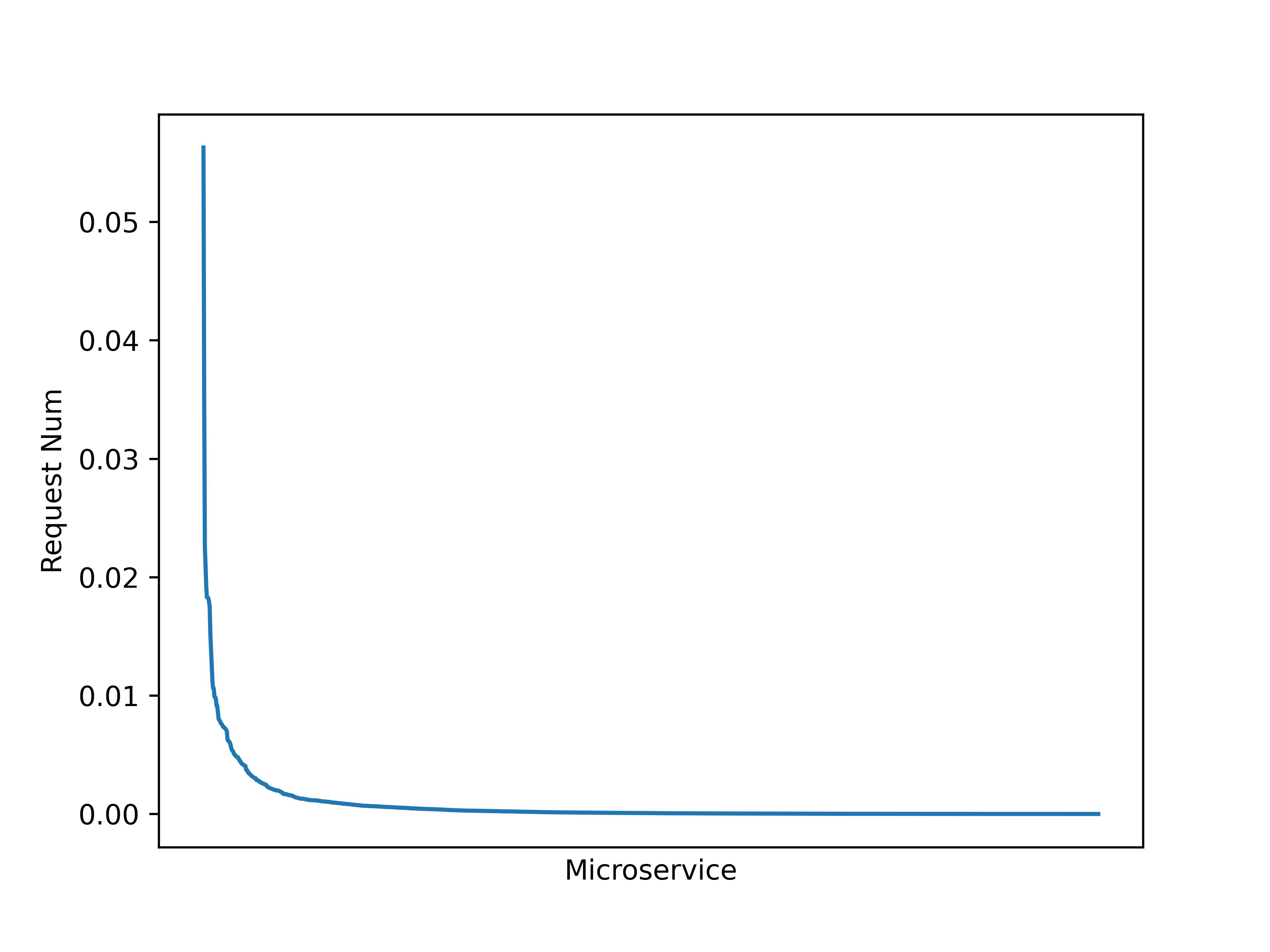
Figure 2: Request Distribution

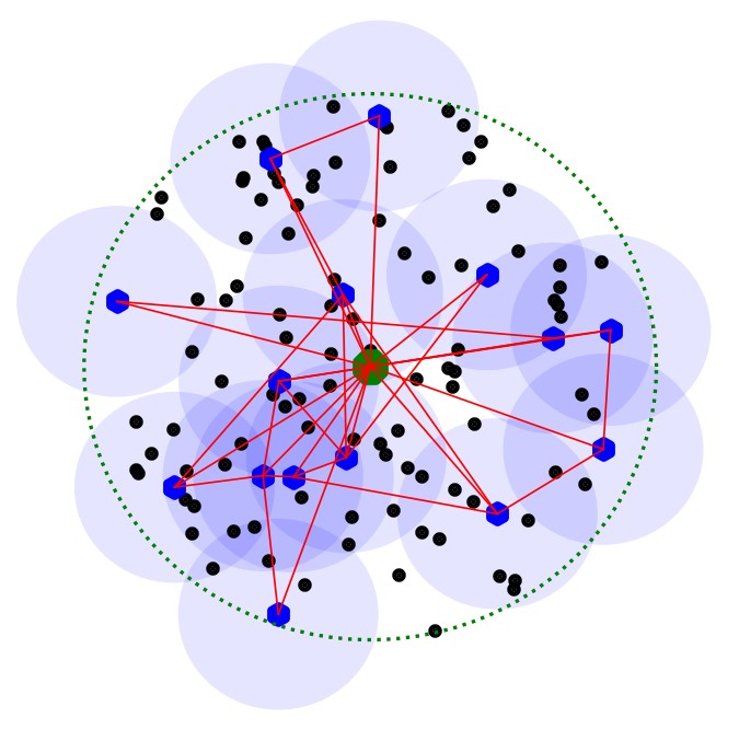
Figure 3: Scenario Sketch

The vertical axis represents the portion of microservices requested during this period, and the horizontal axis represents the transition from the most requested microservice to the least requested one. We can see clearly that the portion of requests for these microservices follows a long-tail distribution. Among the 1300 microservices, the 263 most frequently requested microservices accounted for $90\%$ of user requests. Such a long-tail distribution suggests that it is reasonable in our model to allow some microservice images to be deployed on multiple SCNs and some microservice imaged not to be deployed on the edge. Deploying all kinds of microservices like [GZH⁺21b, GZH⁺21a] is expensive in storage and contributes little to improve users’ experience.

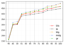
(a) The impact of workload

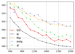
(b) The impact of storage capacity

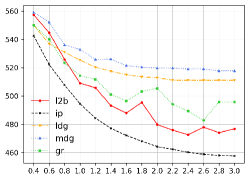
(c) The impact of computation capacity

Figure 4: The impact of (a)workload, (b)storage resource capacity, (c)computation resource capacity on global latency at heterogeneous edge network under first popularity

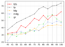
(a) The impact of workload

(b) The impact of storage capacity

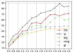
(c) The impact of computation capacity

Figure 5: The impact of (a)workload, (b)storage resource capacity, (c)computation resource capacity on the number of microservice containers at heterogeneous edge network under first popularity

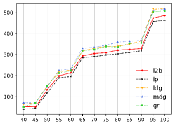
(a) The impact of workload

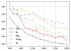
(b) The impact of storage capacity

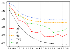
(c) The impact of computation capacity

Figure 6: The impact of (a)workload, (b)storage resource capacity, (c)computation resource capacity on global latency at homogeneous edge network under first popularity

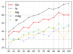
(a) The impact of workload

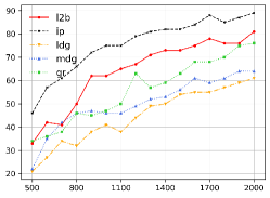
(b) The impact of storage capacity

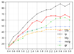
(c) The impact of computation capacity

Figure 7: The impact of (a)workload, (b)storage resource capacity, (c)computation resource capacity on the number of microservice containers at homogeneous edge network under first popularity

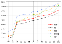
(a) The impact of workload

(b) The impact of storage capacity

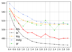
(c) The impact of computation capacity

Figure 8: The impact of (a)workload, (b)storage resource capacity, (c)computation resource capacity on global latency at heterogeneous edge network under second popularity

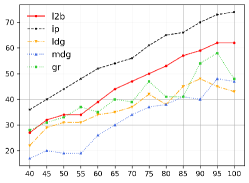
(a) The impact of workload

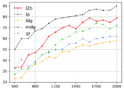
(b) The impact of storage capacity

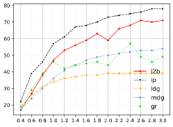
(c) The impact of computation capacity

Figure 9: The impact of (a)workload, (b)storage resource capacity, (c)computation resource capacity on the number of microservice containers at heterogeneous edge network under second popularity

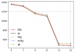
(a) The impact on global latency

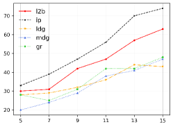
(b) The impact on container number

Figure 10: The impact of SCN density on global latency and the number of microservice containers at heterogeneous edge network under first popularity

5.2 Experiment Settings

We consider an MCN with an effective coverage area of 1km radius, and its storage and computing capacities are 2250BM and 3GHz respectively. In this area, there are 100 users whose location obeys random two-dimensional Poisson distribution. There are 15 SCNs with an effective coverage area of 350m radius whose location also obeys random two-dimensional Poisson distribution but with lower density. The SCNs are directly connected to each other with a certain probability. Considering the practice that two directly connected SCNs are often placed in the same area or close to each other where wired or fast wireless connections can be used [PIA⁺16, AP15]. There is a negative correlation between the probability of edge between two SCNs and the distance between them. Based on above settings, one of the scenarios generated is shown in Fig.3. The SCNs are equipped with finite storage capacity and computing capacity in range 500MB$\sim$1500MB and 1.6GHz$\sim$2.4GHz. In this case, we choose 20 different microservices and they are composed of 116 different layers with size in range 10MB $\sim$ 400MB. Each microservice consists of $4\sim 8$ layers and $12\%\sim 51\%$ of the image are shareable layers. Each microservice required computing resource is in range $\text{0.15GHz}\sim\text{0.45GHz}$. The data size of tasks is randomly distributed between 5 Mbit and 20 Mbit[ZZQ⁺20].

Wireless Communication Model. Our method can be applied to any wireless communication model, this paper chooses a common model to study. We use $p_{u}=23$ dbm to denote the transmitting power of MU-$u$. All the signals experiences path loss with the same loss exponent $\alpha=4$. Therefore, the received power for SCN-$n$ from MU-$u$ is $p_{u}D\|P_{u}-Q_{n}\|^{-\alpha}$, where $D$ denote the channel power gains which are Rayleigh distributed with unitary average power, $D\sim exp(1)$. The power of the noise of all channels is the same $\sigma^{2}=1$. Therefore, the uplink bandwidth can be calculated by Shannon formula as below:

$$E_{u,n}=\begin{cases}W\log_{2}(1+\frac{\delta_{u}H\|P_{u}-Q_{n}\|^{2}}{\sigma^{2}}),&\text{if $\vartheta_{u,n}=1$}\\ 0,&\text{otherwise.}\end{cases}$$

The bandwidth between the SCNs, SCN and MCN, MCN and central cloud are 30 $\sim$ 45 Mbps, 8 $\sim$ 12 Mbps and 20 Mbps respectively[SHND19]. For the wireless upload of user data, we set the channel bandwidth $W$ allocated to a user by SCN or MCN 6MHz[ZKA21].

To evaluate the performance of our algorithm, we have prepared three benchmark algorithms. These benchmarks are used to solve $(\mathcal{P}_{2})$ directly instead of solving $(\mathcal{P}_{1})$.

The benchmark algorithms are Latency Difference Greedy (LDG) algorithm, Microservice Deployment Greedy (MDG) algorithm, Greedy Rounding(GR) algorithm, respectively [GZH⁺21a]. We also explored Random Rounding(RR) algorithm inspired by [GCX⁺22]. Due to the large size of our problem and strong mutual dependency between microservice deployment and task assignment, RR cannot obtain a feasible solution even in hours.

Latency Difference Greedy(LDG). We calculate the difference between the second lowest latency and the lowest latency for each user. The larger the difference is, the higher priority is given the task assignment. In descending order of priority, we assign the task to the SCN with lowest latency and deploy the corresponding microservice.

Microservice Deployment Greedy(MDG). Each SCN preferentially deploys the microservices that are requested more frequently in the coverage area until the storage space is insufficient to deploy more microservice. Then it greedily assigns the user’s task to the available SCN with lowest latency.

Greedy Rounding(GR). This algorithm is inspired by [GZH⁺21a]. This algorithm relaxes $(\mathcal{P}_{2})$ as a LP problem and adopts ADMM to solve it and then greedily rounds the liner solution into integer solution.

In addition, we also present the optimal solution which is called (IP) of $(\mathcal{P}_{2})$ by time-consuming branch and bound algorithm.

We conduct four series of experiments to explore the impact of workload, storage resources, computing resources, and SCN density respectively. The edge networks in the first, third and forth series of experiments are heterogeneous, with each SCN having identical storage and computing capabilities while the edge networks in the second set of experiments are homogeneous. We simulated two different groups of microservice request popularity, respectively based on the distribution of microservice request in two different periods of time in Alibaba’s 2021 trace. The first, second and forth series of experiments are conducted with the first set of microservice popularity while the third experiment is conducted with the second set of microservice popularity.

We first show the impact of workload which can be expressed in terms of the number of users in the area. Fig.4(a), Fig.6(a) and Fig.8(a) show the impact of the workload on the global latency, with the number of users increasing from 40 to 100. As expected, the global latency tends to increase for all algorithms which is a natural phenomenon. These experimental results show that our algorithm outperforms benchmark algorithm and is close to the optimal policy in almost all cases. Comparing Fig.4(a) and Fig.6(a), it shows that under the same workload, the global latency in homogeneous edge networks is always lower than that in the in the heterogeneous network. This seems to indicate that homogeneous edge network may have better performance than heterogeneous edge network. However, this is not always true in other simulation experiments. The main reason is that the workload of each SCN is imbalanced, when the SCNs with more resource cover more user, grater portion of user can enjoy low-latency web service from nearby SCN. As shown in Fig.5(a), Fig.7(a) and Fig.9(a) with the increase of workload, more microservice container are running to provide web service. However, even when workload is low, the number of running containers is significantly smaller than the number of users. That is the storage capacity is the bottleneck of performance in this case so that some requested microservices are not deployed in the edge. Even though there are sufficient computing resource remains, tasks are still needed to be assigned to the central cloud.

Then we consider the average storage of SCNs varying from 500MB to 2000MB in Fig4(b), Fig6(b) and Fig8(b). As expected, increasing storage capacity will make the global latency tend to decrease for all algorithms because more kinds of microservice and more replicas can be deployed in the edge. More users can enjoy web service from a nearby SCN with low latency. The experiment results show that both in homogeneous networks and in the heterogeneous network, our algorithm outperforms other algorithms. In addition, the results show that the rate of latency reduction slows down as storage resources increase. This is because the limited computing resources gradually become the main factor affecting the performance improvement after the storage becomes sufficient. Fig.5(b), Fig.7(b) and Fig.9(b) show that as the storage resource increases, the number of containers running in the edge network also increase, which conforms our interpretation of the global latency decrease. It’s noticing that when storage capacity varies from 1600MB to 2000MB, the number of containers running in the edge decreases. The reason for this phenomenon is that the rounding strategy in the second step is heuristic which sometimes may outputs a relatively poor result.

Next, we explore the impact of computation capacity in Fig.4(c), Fig.6(c) and Fig.8(c). The average computation capacity varies from 0.5GHz to 3.0GHz. The global latency tends to decrease for all algorithms as the computational power increases. This is because the SCN can start more containers to provide service. The experiment results also show that the solution of our proposed algorithm is better than all other algorithms. In addition, the results show that the rate of latency reduction slows down as computing resources increase. This is because the limited storage resources gradually become the main factor affecting the performance improvement after the computing resource becomes sufficient. As shown in Fig.5(c), Fig.7(c) and Fig.9(c), our algorithm can run more containers in the edge in most situations. As a result of our optimization goal is global delay, the more the number of tasks performed on the edge of the network, does not necessarily mean lower latency.

Last but not least, we will show the effect of SCN density in Fig.10(a) and Fig.10(b). As the number of SCNs increases from 5 to 15, the global latency decreases. One reason is that, as shown in Fig.10(b), with the increase of the number of SCNs, the total computing resource of the edge network increases, and more users are served by the edge. Another reason is that more users can uploading data to a nearby SCN instead of uploading data to MCN with longer latency. As the number of SCNs grows from 11 to 13, the global latency decreases sharply while the number of containers increases gently. After analyzing, it is found that SCN-$12$ just covers a large number of users at the edge of the area who are covered only by MCN before. They suffer terrible network condition when they upload their data to MCN. SCN-$12$ enables them to enjoy low latency web service. This phenomenon just validates our second explanation for the latency reduction.

6 Conclusion

In this paper, we consider both 5G edge network with densely deployed SCNs and the prominent layer structure of microservice. To study microservice deployment, layer deployment, AP selection and task assignment, we formulate a BQP problem ($\mathcal{P}_{1}$) to minimize the global latency. We decompose it and transform it to an ILP form ($\mathcal{P}_{2}$). We propose sphere-box ADMM and a heuristic rounding policy to solve it. By analyzing alibaba’s trace, we design simulation experiments. And the results show the efficiency of our algorithm.

Haojie Yan received the B.Eng. degree from the School of Information Science and Technology, Fudan University, Shanghai, China, in 2021. He is currently pursuing the M.S. degree at Fudan University, Shanghai, China. His research interests include deep reinforcement learning, mixed integer programming.

Yuedong Xu received the B.S. degree from Anhui University, the M.S. degree from the Huazhong University of Science and Technology, and the Ph.D. degree from The Chinese University of Hong Kong. From 2009 to 2012, he held a post-doctoral position with INRIA Sophia Antipolis and Universite d’Avignon, France. He is a Professor with the School of Information Science and Technology, Fudan University, China. He has published nearly 20 conference and journal papers in premium vents such as CoNEXT, Mobisys, Mobihoc, Infocom and IEEE/ACM ToN. His research interests include performance evaluation, optimization, machine learning and economic analysis of communication networks and mobile computing.

Liangui Dai Liangui Dai received Ph.D. degree in Control Theory and Application from Northeastern University, ShenYang, China in 1997. He is a senior researcher with the intelligent transportation system (ITS) research institute of Guangdong Litong Corp. His research interests include data analytics of ITS and information system development for ITS.

Appendix A Specific definition fro matrix and vector

There are $N$ inequation in constraint 2. We can use a matrix $\mathbf{\Psi}_{n,nL+l}^{1}=K_{l}$ and a vector $\bm{\tau}^{1}=\mathbf{S}$ to rewritten them as a compact form as follows:

$$\mathbf{\Psi}^{1}\bm{y}\leq\bm{\tau}^{1}.$$ (18)

There are $LI$ inequality constraints in constraint 3. We user a matrix $\mathbf{\Phi}^{2}_{nIL+iL+l,nI+i}=H_{i,l}$, $\mathbf{\Psi}_{2}(nIL+iL+l,nL+l)=-1$ and a vector $\bm{\tau}^{2}=\mathbf{0}$to rewrite constraints as below compact form:

$$\mathbf{\Phi}^{2}\bm{x}+\mathbf{\Psi}^{2}\bm{y}\leq\bm{\tau}^{2}.$$ (19)

We can use the matrix $\mathbf{\Omega}^{3}_{n,n(N+2)+n}=1$ and vector $\bm{\tau}^{3}=\mathbf{1}$ to rewrite the equations in constraint (6) as following compact form:

$$\mathbf{\Omega}^{3}\bm{w}=\bm{\tau}^{3}.$$ (20)

By defining matrix $\mathbf{\Phi}^{4}_{u(N+1)n,M_{u}}=-1$, matrix $\mathbf{\Omega}^{4}_{u(N+1)+n,u(N+2)+n}=1$ and vector $\bm{\tau}^{4}=\mathbf{0}_{U(N+2)}$, constraints in (7) can be reorganized as following:

$$\mathbf{\Phi}^{4}\bm{x}+\mathbf{\Omega}^{4}\bm{w}\leq\bm{\tau}^{4}.$$ (21)

Considering matrix $\mathbf{\Omega}^{5}_{n,u(N+2)+n}=F_{M_{u}}$ and vector $\bm{\tau}^{5}=\mathbf{C}$, we obtain the equivalent expression of constraint (8):

$$\mathbf{\Omega}^{5}\mathbf{w}\leq\bm{\tau}^{5}.$$ (22)

We introduce positive auxiliary variables $\bm{h}_{1}$, $\bm{h}_{2}$, $\bm{h}_{4}$ and $\bm{h}_{5}$ to transform the inequality constraints in constraint (18),(19),(21),(22) to equality constraints:

$$\mathbf{\Psi}^{1}\bm{y}+\bm{h}_{1} =\bm{\tau}^{1},\text{ }\bm{h}_{1}\in\mathbb{R}_{+}^{(N+1)},$$ (23)

$$\mathbf{\Phi}^{2}\bm{x}+\mathbf{\Psi}^{2}\bm{y}+\bm{h}_{2} =\bm{\tau}^{2},\text{ }\bm{h}_{2}\in\mathbb{R}_{+}^{(N+1)ML},$$ (24)

$$\mathbf{\Phi}^{4}\bm{x}+\mathbf{\Omega}^{4}\bm{w}+\bm{h}_{4} =\bm{\tau}^{4},\text{ }\bm{h}_{4}\in\mathbb{R}_{+}^{U(N+1)},$$ (25)

$$\mathbf{\Omega}^{5}\bm{w}+\bm{h}_{5} =\bm{\tau}^{5},\text{ }\bm{h}_{5}\in\mathbb{R}_{+}^{(N+1)}.$$ (26)

Based on the above definition, the matrixes and vectors in ($\mathcal{P}_{3}$) are defined as following:

$$\mathbf{f}^{\top}\bm{v}=\displaystyle\sum_{u=1}^{U}\sum_{m=1}^{N+2}\xi_{u,m}w_{u,m},$$

$$\mathbf{A}_{1}=\begin{bmatrix}\text{\Large 0}&\text{\Large 0}&\mathbf{\Omega}_{3}\end{bmatrix},$$

$$\mathbf{A}_{2}=\begin{bmatrix}\text{\Large 0}&\mathbf{\Psi}^{1}&\text{\Large 0}\\ \mathbf{\Phi}^{2}&\mathbf{\Psi}^{2}&\text{\Large 0}\\ \mathbf{\Phi}^{4}&\text{\Large 0}&\mathbf{\Omega}^{4}\\ \text{\Large 0}&\text{\Large 0}&\mathbf{\Omega}^{5}\end{bmatrix},$$

$$\mathbf{g}_{1}=[\bm{\tau}^{3}]^{\top},$$

$$\mathbf{g}_{2}=[\bm{\tau}^{1},\bm{\tau}^{2},\bm{\tau}^{4},\bm{\tau}^{5}]^{\top},$$

$$\mathbf{h}=[\mathbf{h}_{1},\mathbf{h}_{2},\mathbf{h}_{4},\mathbf{h}_{5}]^{\top}.$$

Appendix B Notations

Notation	Meaning
$\mathcal{N}$	Set of SCNs
$\mathcal{U}$	Set of users
$\mathcal{I}$	Set of microservices
$\mathcal{L}$	Set of layers
$S_{n}$	Storage capacity of SCN-$n$
$C_{n}$	Computation capacity of SCN-$n$
$P_{n}$	Place of SCN-$n$
$B_{n,m}$	Bandwidth between SCN-$n$ and SCN-$m$
$H_{i,l}$	Indicator whether layer-$l$ is required by MS-$i$
$K_{l}$	Size of layer-$l$
$F_{i}$	Required computation by MS-$i$
$Q_{n}$	The place of MU-$n$
$M_{u}$	The microservice requested by MU-$u$
$R_{u}$	The size of data which MU-$u$ want to process
$p_{u}$	The transmitting power of MU-$u$’s device
$W_{u,n}$	The bandwidth between MU-$u$ and SCN-$n$
$x_{u,i}$	Decision variable whether SCN-$n$ deploys MS-$i$
$y_{n,l}$	Decision variable whether SCN-$n$ deploys layer-$l$
$z_{u,n}$	Decision variable whether MU-$u$ connets to SCN-$n$
$w_{u,m}$	Decision variable whether MU-$u$’s task is assigned to SCN-$m$
$\vartheta_{u,n}$	Indicator whether MU-$u$ can connect to SCN-$n$
$\mathit{G}$	Topology of the edge network
$\xi_{u,m}$	The lowest latency from MU-$u$ to SCN-$m$
$\zeta_{u,m}$	The SCN which MU-$u$ connects when $xi_{u,m}$ is achieved
$q$	The number of variable in $(\mathcal{P}_{2})$
$D$	Wireless channel power gain
$\alpha$	Wireless path channel loss

References

- [AP15] Weng Chon Ao and Konstantinos Psounis. Distributed caching and small cell cooperation for fast content delivery. In Proceedings of the 16th ACM international symposium on mobile ad hoc networking and computing, pages 127–136, 2015.
- [FFRR15] Wes Felter, Alexandre Ferreira, Ram Rajamony, and Juan Rubio. An updated performance comparison of virtual machines and linux containers. In 2015 IEEE international symposium on performance analysis of systems and software (ISPASS), pages 171–172. IEEE, 2015.
- [GCX+22] Lin Gu, Zirui Chen, Honghao Xu, Deze Zeng, Bo Li, and Hai Jin. Layer-aware collaborative microservice deployment toward maximal edge throughput. In IEEE INFOCOM 2022-IEEE Conference on Computer Communications, pages 71–79. IEEE, 2022.
- [GZH+21a] Lin Gu, Deze Zeng, Jie Hu, Hai Jin, Song Guo, and Albert Y Zomaya. Exploring layered container structure for cost efficient microservice deployment. In IEEE INFOCOM 2021-IEEE Conference on Computer Communications, pages 1–9. IEEE, 2021.
- [GZH+21b] Lin Gu, Deze Zeng, Jie Hu, Bo Li, and Hai Jin. Layer aware microservice placement and request scheduling at the edge. In IEEE INFOCOM 2021-IEEE Conference on Computer Communications, pages 1–9. IEEE, 2021.
- [HH18] Lih-Tyng Hwang and Tzyy-sheng Jason Horng. 3D IC and RF SiPs: Advanced Stacking and Planar Solutions for 5G Mobility. John Wiley & Sons, 2018.
- [HNN+18] Dinh Thai Hoang, Dusit Niyato, Diep N Nguyen, Eryk Dutkiewicz, Ping Wang, and Zhu Han. A dynamic edge caching framework for mobile 5g networks. IEEE Wireless Communications, 25(5):95–103, 2018.
- [HSL+16] Tyler Harter, Brandon Salmon, Rose Liu, Andrea C Arpaci-Dusseau, and Remzi H Arpaci-Dusseau. Slacker: Fast distribution with lazy docker containers. In 14th USENIX Conference on File and Storage Technologies (FAST 16), pages 181–195, 2016.
- [KFF+18] Sami Kekki, Walter Featherstone, Yonggang Fang, Pekka Kuure, Alice Li, Anurag Ranjan, Debashish Purkayastha, Feng Jiangping, Danny Frydman, Gianluca Verin, et al. Mec in 5g networks. ETSI white paper, 28(2018):1–28, 2018.
- [LAMC19] Yan Li, Bo An, Junming Ma, and Donggang Cao. Comparison between chunk-based and layer-based container image storage approaches: an empirical study. In 2019 IEEE International Conference on Service-Oriented System Engineering (SOSE), pages 197–1975. IEEE, 2019.
- [LHL+21] Quyuan Luo, Shihong Hu, Changle Li, Guanghui Li, and Weisong Shi. Resource scheduling in edge computing: A survey. IEEE Communications Surveys & Tutorials, 23(4):2131–2165, 2021.
- [LXL+21] Shutian Luo, Huanle Xu, Chengzhi Lu, Kejiang Ye, Guoyao Xu, Liping Zhang, Yu Ding, Jian He, and Chengzhong Xu. Characterizing microservice dependency and performance: Alibaba trace analysis. In Proceedings of the ACM Symposium on Cloud Computing, pages 412–426, 2021.
- [LYCT17] Kuikui Li, Chenchen Yang, Zhiyong Chen, and Meixia Tao. Optimization and analysis of probabilistic caching in -tier heterogeneous networks. IEEE Transactions on Wireless Communications, 17(2):1283–1297, 2017.
- [ÖBT10] Lale Özbakir, Adil Baykasoğlu, and Pınar Tapkan. Bees algorithm for generalized assignment problem. Applied Mathematics and Computation, 215(11):3782–3795, 2010.
- [PIA+16] Konstantinos Poularakis, George Iosifidis, Antonios Argyriou, Iordanis Koutsopoulos, and Leandros Tassiulas. Caching and operator cooperation policies for layered video content delivery. In IEEE INFOCOM 2016-The 35th Annual IEEE International Conference on Computer Communications, pages 1–9. IEEE, 2016.
- [PIST16] Konstantinos Poularakis, George Iosifidis, Vasilis Sourlas, and Leandros Tassiulas. Exploiting caching and multicast for 5g wireless networks. IEEE Transactions on Wireless Communications, 15(4):2995–3007, 2016.
- [RN16] Flávio Ramalho and Augusto Neto. Virtualization at the network edge: A performance comparison. In 2016 IEEE 17th International Symposium on A World of Wireless, Mobile and Multimedia Networks (WoWMoM), pages 1–6. IEEE, 2016.
- [SHND19] Yuris Mulya Saputra, Dinh Thai Hoang, Diep N Nguyen, and Eryk Dutkiewicz. A novel mobile edge network architecture with joint caching-delivering and horizontal cooperation. IEEE Transactions on Mobile Computing, 20(1):19–31, 2019.
- [SJMW19] Amit Samanta, Lei Jiao, Max Mühlhäuser, and Lin Wang. Incentivizing microservices for online resource sharing in edge clouds. In 2019 IEEE 39th International Conference on Distributed Computing Systems (ICDCS), pages 420–430. IEEE, 2019.
- [WG18] Baoyuan Wu and Bernard Ghanem. p-box admm: A versatile framework for integer programming. IEEE transactions on pattern analysis and machine intelligence, 41(7):1695–1708, 2018.
- [WLZ+18] Liang Wang, Mengyuan Li, Yinqian Zhang, Thomas Ristenpart, and Michael Swift. Peeking behind the curtains of serverless platforms. In 2018 USENIX Annual Technical Conference (USENIX ATC 18), pages 133–146, 2018.
- [ZKA21] Yongqiang Zhang, Mustafa A Kishk, and Mohamed-Slim Alouini. Computation offloading and service caching in heterogeneous mec wireless networks. IEEE Transactions on Mobile Computing, 22(6):3241–3256, 2021.
- [ZZQ+20] Ruiting Zhou, Xueying Zhang, Shixin Qin, John CS Lui, Zhi Zhou, Hao Huang, and Zongpeng Li. Online task offloading for 5g small cell networks. IEEE Transactions on Mobile Computing, 21(6):2103–2115, 2020.