1 Introduction

1.1 Poincaré spinor

Any uniform plane wave propagating in free space can be represented as a point on the surface of the Poincaré sphere $s_{1}^{2}+s_{2}^{2}+s_{3}^{2}=s_{0}^{2}$, where $s_{0}$, $s_{1}$, $s_{2}$, and $s_{3}$ are the four Stokes parameters. The plane wave’s location is identified by the longitude $\alpha\in[0,2\pi)$ and the latitude $\beta\in[-\pi/2,\pi/2]$ defined through the relations

$$\left.\begin{array}[]{l}s_{1}=s_{0}\,\cos\beta\,\cos\alpha\\[5.0pt] s_{2}=s_{0}\,\cos\beta\,\sin\alpha\\[5.0pt] s_{3}=s_{0}\,\sin\beta\end{array}\right\}\,,$$ (1)

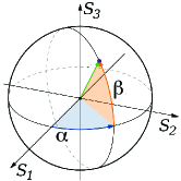
Figure 1: Longitude $\alpha\in[0,2\pi)$ and latitude $\beta\in[-\pi/2,\pi/2]$ that identify a plane wave on the Poincaré sphere.

as shown in Fig. 1. These two angles appear in the Poincaré spinor

$$\left[{\underline{\phi}}\right]=\left[\begin{array}[]{c}\cos\left(\frac{\pi}{4}-\frac{\beta}{2}\right)\\[5.0pt] \sin\left(\frac{\pi}{4}-\frac{\beta}{2}\right)\exp\left(i\alpha\right)\end{array}\right]\,,$$ (2)

where $i=\sqrt{-1}$.

1.2 Geometric phase

With respect to a plane wave labeled “1”, the geometric phase of a plane wave labeled “2” is defined as the angle

$$\Phi_{21}={\rm Arg}\left\{{\left[{\underline{\phi}}_{1}\right]}^{\dagger}\cdot{\left[{\underline{\phi}}_{2}\right]}\right\}\,,$$ (3)

where ^† denotes the conjugate transpose. The geometric phase is a measure of dissimilarity of two plane waves of the same frequency, even when propagating in the same direction, as was pointed out by Pancharatnam in 1956 [1]. The profound role of geometric phase in classical as well as quantum physics was recognized within the next three decades [2] and it continues to both fascinate researchers [3, 4] and find applications [6, 5, 7, 8].

Optical experiments on plane-wave transmission through a columnar thin film [9] and a chiral sculptured thin film [10] have revealed that the geometric phase of the transmitted plane wave depends on the morphology of the thin film [11]. Thin-film morphology can be architected using a variety of fabrication techniques including physical vapor deposition [10, 12], holographic lithography [13], direct laser writing [14], electron tomography [15], hydrothermal method [16], and self assembly [17, 18]. Each technique may produce thin films with similar plane-wave reflectance and transmittance characteristics, but the geometric phase of the reflected and/or transmitted plane wave could contain a signature of the fabrication technique.

1.3 Reusch piles

An experimental test of the foregoing proposition requires resources presently unavailable to me. So, I chose to establish the rudiments of this proposition theoretically. Chiral sculptured thin films may be considered to be finely chiral Reusch piles [19]. Conceived in 1869 [20], a Reusch pile is a periodic multilayer comprising layers of the same homogeneous, uniaxial dielectric material, such that the optic axis in each layer is rotated about the thickness direction (designated to be parallel to the $z$ axis of a Cartesian coordinate system) with respect to the optic axis in the previous layer by a fixed angle $\Delta\xi$. A delightful artistic interpretation of Reusch piles is available from the sculpture Seque created by Anne Huibregtse [21].

A Reusch pile preferentially reflects light of one circular-polarization state in multiple spectral regimes [22], preserving the circular-polarization state of the incident plane wave [23]. These spectral regimes, called circular Bragg regimes [24], depend on both the number of layers in one period of the Reusch pile and the dependencies of the constitutive parameters on the frequency [19].

The following classification of Reusch piles was devised in 2004 [19]: Suppose that the period $P$ of a Reusch pile is made up of $2q$, $q\geq 2$, identical layers stacked along the $z$ axis. Then the angular offset of the optic axis of a specific layer with respect to the optic axis of the previous layer is given by

$$\Delta\xi=h\frac{\pi}{q}\,,\quad q\in\left\{{2,3,4,\dots}\right\}\,,$$ (4)

where $h=+1$ for structural right-handedness and $h=-1$ for structural left-handedness. With the assumption that the constitutive parameters are independent of frequency (which is an approximation of limited physical validity [25]), the Reusch pile shall display two families of circular Bragg regimes. Circular Bragg regimes in the first family are conjectured to exist with center wavelengths

$$\lambda_{\scriptscriptstyle 0}^{1;p,q}=\frac{\lambda_{\scriptscriptstyle 0}^{1;0,q}}{pq+1}\,,\qquad p\in\left\{{0,1,2,3,\dots}\right\}\,,\quad q\in\left\{{2,3,4,\dots}\right\}\,,$$ (5)

whereas circular Bragg regimes in the second family are predicted with center wavelengths

$$\lambda_{\scriptscriptstyle 0}^{2;p,q}=\frac{\lambda_{\scriptscriptstyle 0}^{1;0,q}}{pq+q-1}\,,\qquad p\in\left\{{0,1,2,3,\dots}\right\}\,,\quad q\in\left\{{2,3,4,\dots}\right\}\,,$$ (6)

where $\lambda_{\scriptscriptstyle 0}^{1;0,q}$ depends on the constitutive parameters and period of the Reusch pile and normal incidence has been assumed. Equations (5) and (6) will require modification for frequency-dependent constitutive parameters [27, 26]. Furthermore, there may be other circular Bragg regimes that are not captured by the conjectures (5) and (6).

When $h=1$ and the Reusch pile has a sufficiently large number of periods, the reflectance of an incident right-circularly polarized (RCP) plane wave is very high but that of an incident left-circularly polarized (LCP) plane wave is very low in the first family of circular Bragg regimes, whereas the reflectance of an incident LCP plane wave is very high but that of an incident RCP plane wave is very low in the second family. When $h=-1$ and the Reusch pile has a sufficiently large number of periods, the reflectance of an incident LCP plane wave is very high but that of an incident RCP plane wave is very low in the first family, whereas the reflectance of an incident RCP plane wave is very high but that of an incident LCP plane wave is very low in the second family of circular Bragg regimes.

Since $\lambda_{\scriptscriptstyle 0}^{1;p,2}=\lambda_{\scriptscriptstyle 0}^{2;p,2}\,\forall{p}$, the Reusch pile is classified as equichiral for $q=2$. If $q\geq 3$, the Reusch pile is classified as ambichiral. As $q\to\infty$, the Reusch pile is finely chiral with reflectance and transmittance characteristics similar to that chiral liquid crystals [28, 29, 30, 31] and chiral sculptured thin films [10, 32, 33]. Equichiral Reusch piles exhibit the Bragg phenomenon without differentiating between LCP and RCP plane waves [19, 34], as has been experimentally verified [35].

Given that $\lambda_{\scriptscriptstyle 0}^{1;p+1,q}<\lambda_{\scriptscriptstyle 0}^{1;p,q}$ and $\lambda_{\scriptscriptstyle 0}^{2;p+1,q}<\lambda_{\scriptscriptstyle 0}^{2;p,q}$, it would be arduous to experimentally verify the multiplicity of circular Bragg regimes with a single Reusch pile if $\lambda_{\scriptscriptstyle 0}^{1;0,q}$ lies in the visible regime. Still, the exhibition of two adjacent circular Bragg regimes, the ones for $p=0$ from both families with $q$ fixed, has been experimentally confirmed with some deviation from Eq. (6) due to frequency dependence of the constitutive parameters [19, 36].

1.4 Architected morphology

With fixed $P$ but increasing $q$, Reusch piles offer an evolutionary perspective on the roles that architected morphology can play in diverse optical phenomena. Such studies have been undertaken for transmission-mode optical activity [37, 23, 38], circular Bragg phenomenon [36, 39, 40], and surface-wave propagation [41]. In this chapter, I deploy Reusch piles to study the evolution of the geometric phases of the reflected and transmitted plane waves when a Reusch pile is illuminated by a plane wave.

The 2004 classification [19] of Reusch piles excludes (i) columnar thin films [9, 10] and (ii) chevronic sculptured thin films [42], because these materials with architected morphology do not exhibit the circular Bragg phenomenon. But their inclusion is necessary to understand the relationship, or lack thereof, between the geometric phase and morphology. Therefore, I augmented Eq. (4) to

$$\Delta\xi=h\frac{2\pi}{\tilde{N}}\,,\quad\tilde{N}\in\left\{{1,2,3,4,\dots}\right\}\,.$$ (7)

Whereas $\tilde{N}=1$ for columnar thin films and $\tilde{N}=2$ for chevronic thin films, $\tilde{N}=4$ for equichiral Reusch piles and $\tilde{N}\in\left\{{6,8,10,\dots}\right\}$ for ambichiral Reusch piles in the 2004 classification [19]. In addition, $\tilde{N}\in\left\{3,5,7,\dots\right\}$, which were not explicitly included in the 2004 classification, are also possible while maintaining a full turn of $2\pi$ of the optic axes within the thickness $P$.

The conjectures (5) and (6) still apply with $q$ replaced by $\tilde{N}/2$, $\tilde{N}\in\left\{{2,3,4,\dots}\right\}$. The case of $\tilde{N}=1$ has to be excluded, because a columnar thin film lacks periodicity. Equation (5) indicates that

$$\frac{\lambda_{\scriptscriptstyle 0}^{1;p,\tilde{N}/2}}{\lambda_{\scriptscriptstyle 0}^{1;0,\tilde{N}/2}}\in\left\{\begin{array}[]{l}\left\{1,\frac{1}{2},\frac{1}{3},\frac{1}{4},\dots\right\}\,,\\[5.0pt] \left\{1,\frac{2}{5},\frac{2}{8},\frac{2}{11},\dots\right\}\,,\\[5.0pt] \left\{1,\frac{1}{3},\frac{1}{5},\frac{1}{7},\dots\right\}\,,\\[5.0pt] \left\{1,\frac{2}{7},\frac{2}{12},\frac{2}{17},\dots\right\}\,,\\[5.0pt] \left\{1,\frac{1}{4},\frac{1}{7},\frac{1}{10},\dots\right\}\,,\end{array}\right.\qquad\tilde{N}=\left\{\begin{array}[]{l}2\\[5.0pt] 3\\[5.0pt] 4\\[5.0pt] 5\\[5.0pt] 6\end{array}\right.\,,$$ (8)

and

$$\frac{\lambda_{\scriptscriptstyle 0}^{2;p,\tilde{N}/2}}{\lambda_{\scriptscriptstyle 0}^{1;0,\tilde{N}/2}}\in\left\{\begin{array}[]{l}\left\{\infty,1,\frac{1}{2},\frac{1}{3},\dots\right\}\,,\\[5.0pt] \left\{2,\frac{2}{4},\frac{2}{7},\frac{2}{10},\dots\right\}\,,\\[5.0pt] \left\{1,\frac{1}{3},\frac{1}{5},\frac{1}{7},\dots\right\}\,,\\[5.0pt] \left\{\frac{2}{3},\frac{2}{8},\frac{2}{13},\frac{2}{18},\dots\right\}\,,\\[5.0pt] \left\{\frac{1}{2},\frac{1}{5},\frac{1}{8},\frac{1}{11},\dots\right\}\,,\end{array}\right.\qquad\tilde{N}=\left\{\begin{array}[]{l}2\\[5.0pt] 3\\[5.0pt] 4\\[5.0pt] 5\\[5.0pt] 6\end{array}\right.\,,$$ (9)

Thus, the largest finite value of $\lambda_{\scriptscriptstyle 0}^{\ell;p,\tilde{N}/2}$, $\ell\in\left\{1,2\right\}$, is $\lambda_{\scriptscriptstyle 0}^{1;0,\tilde{N}/2}$ with one exception: $\lambda_{\scriptscriptstyle 0}^{2;0,3/2}=2\lambda_{\scriptscriptstyle 0}^{1;0,3/2}$. Note that $\lambda_{\scriptscriptstyle 0}^{1;p,1}=\lambda_{\scriptscriptstyle 0}^{2;p+1,1}$ for chevronic thin films and $\lambda_{\scriptscriptstyle 0}^{1;p,2}=\lambda_{\scriptscriptstyle 0}^{2;p,2}$ for equichiral Reusch piles, both instances of the two families of circular Bragg regimes not being distinct from each other in their center wavelengths. The sequences in conjectures (8) and (9) will change when the frequency dependence of the constitutive parameters cannot be ignored.

This chapter is organized as follows. Section 2 provides the theoretical framework to calculate the geometric phase of the reflected/transmitted plane wave in relation to the incident plane wave. Numerical results are presented and discussed in Sec. 3, and the paper ends with key conclusions in Sec. 4. An $\exp(-i\omega t)$ dependence on time $t$ is implicit, where $\omega$ as the angular frequency. With $\varepsilon_{\scriptscriptstyle 0}$ and $\mu_{\scriptscriptstyle 0}$, respectively, denoting the permittivity and permeability of free space, the free-space wavenumber is denoted by $k_{\scriptscriptstyle 0}=\omega\sqrt{\varepsilon_{\scriptscriptstyle 0}\mu_{\scriptscriptstyle 0}}$, and $\lambda_{\scriptscriptstyle 0}=2\pi/k_{\scriptscriptstyle 0}$ is the free-space wavelength. The Cartesian coordinate system $(x,y,z)$ is adopted. Vectors are in boldface and unit vectors are additionally decorated by a caret on top. Dyadics are double underlined. Column vectors are underlined and enclosed in square brackets. Matrixes are double underlined and enclosed in square brackets.

2 Theory

2.1 Relative permittivity dyadic

The Reusch pile is taken to occupy the region $0<z<NP$, where $N\in\left\{1,2,3,\dots\right\}$ is the number of periods, and the relative permittivity dyadic

$$\underline{\underline{\varepsilon}}_{\rm rel}(z+P)=\underline{\underline{\varepsilon}}_{\rm rel}(z)\,,\quad 0<z<(N-1)P\,$$ (10)

is therefore periodic.

The reference unit cell $0<z<P$ is subdivided into $\tilde{N}$ layers. The $n$-th layer, $n\in\left\{1,2,\dots,\tilde{N}\right\}$, is delimited by the planes $z=z_{n-1}$ and $z=z_{n}$, where

$$z_{m}=m\frac{P}{\tilde{N}}\,,\quad m\in\left\{0,1,2,\dots,\tilde{N}\right\}\,.$$ (11)

The relative permittivity dyadic in the $n$-th layer of the reference unit cell is given by

$$\underline{\underline{\varepsilon}}_{\rm rel}(z) = \underline{\underline{Z}}(h;n,\tilde{N})\mbox{ \tiny{${}^{\bullet}$} }\underline{\underline{Y}}(\chi)\mbox{ \tiny{${}^{\bullet}$} }\left[\varepsilon_{\rm a}\hat{{\bf z}}\hat{{\bf z}}+\varepsilon_{\rm b}\hat{{\bf x}}\hat{{\bf x}}+\varepsilon_{\rm c}\hat{{\bf y}}\hat{{\bf y}}\right]\mbox{ \tiny{${}^{\bullet}$} }\underline{\underline{Y}}^{-1}(\chi)\mbox{ \tiny{${}^{\bullet}$} }\underline{\underline{Z}}^{-1}(h;n,\tilde{N})\,,$$ (12)

$$z_{n-1}<z<z_{n}\,,\quad n\in\left\{1,2,\dots,\tilde{N}\right\}\,.$$

The frequency-dependent relative permittivity scalars $\varepsilon_{\rm a}$, $\varepsilon_{\rm b}$, and $\varepsilon_{\rm c}$ capture the orthorhombicity [10] of each layer. The tilt dyadic

$$\underline{\underline{Y}}(\chi)=\hat{{\bf y}}\hat{{\bf y}}+\left(\hat{{\bf x}}\hat{{\bf x}}+\hat{{\bf z}}\hat{{\bf z}}\right)\cos\chi+\left(\hat{{\bf z}}\hat{{\bf x}}-\hat{{\bf x}}\hat{{\bf z}}\right)\sin\chi$$ (13)

contains $\chi\in[{0,\pi/2}]$ as an angle of inclination with respect to the $xy$ plane. The structural handedness is captured by the rotation dyadic

$$\underline{\underline{Z}}(h;n,\tilde{N})=\hat{{\bf z}}\hat{{\bf z}}+\left(\hat{{\bf x}}\hat{{\bf x}}+\hat{{\bf y}}\hat{{\bf y}}\right)\cos\left[{(n-1)h\frac{2\pi}{\tilde{N}}}\right]+\left(\hat{{\bf y}}\hat{{\bf x}}-\hat{{\bf x}}\hat{{\bf y}}\right)\sin\left[{(n-1)h\frac{2\pi}{\tilde{N}}}\right]\,,$$

$$\qquad n\in\left\{1,2,\dots,\tilde{N}\right\}\,.$$ (14)

Examination of Eq. (12) reveals the absence of periodicity only for $\tilde{N}=1$. However, the structural period is not always $P$ for all values of $\chi$. The structural period is $P$ for $\chi\in(0,\pi/2)$, but $P/2$ for $\chi\in\left\{0,\pi/2\right\}$. This distinction has been partially noted earlier [43] for continuously chiral materials (i.e., in the limit $\tilde{N}\to\infty$).

Examination of Eq. (12) reveals also the absence of structural handedness for $\tilde{N}\in\left\{1,2\right\}$. Additionally, structural handedness is absent for $\tilde{N}=4$ provided that $\chi\in\left\{0,\pi/2\right\}$.

2.2 Boundary-Value Problem

The half-space $z<0$ is the region of incidence and reflection, while the half-space $z>L$ is the region of transmission. A plane wave, propagating in the half–space $z\leq 0$ at an angle $\theta_{\rm inc}\in[0,\pi/2)$ with respect to the $z$ axis and at an angle $\psi\in[0,2\pi)$ with respect to the $x$ axis in the $xy$ plane, is incident on the Reusch pile. The electric field phasor associated with the incident plane wave is represented as [10]

$${\bf E}^{\rm inc}({\bf r}) = \left[\frac{\left(i{\bf s}-{\bf p}_{+}\right)}{\sqrt{2}}\,a_{\rm L}-\,\frac{\left(i{\bf s}+{\bf p}_{+}\right)}{\sqrt{2}}\,a_{\rm R}\right]\exp{\left[i\kappa\left(x\cos\psi+y\sin\psi\right)\right]}\exp{\left(ik_{\scriptscriptstyle 0}z{\cos\theta_{\rm inc}}\right)}$$ (15a)

$$= \left(a_{\rm s}{\bf s}+a_{\rm p}{\bf p}_{+}\right)\exp{\left[i\kappa\left(x\cos\psi+y\sin\psi\right)\right]}\exp{\left(ik_{\scriptscriptstyle 0}z{\cos\theta_{\rm inc}}\right)}\,,\qquad z<0\,,$$ (15b)

where

$$\left.\begin{array}[]{l}\kappa=k_{\scriptscriptstyle 0}\sin{\theta_{\rm inc}}\\[5.0pt] {\bf s}=-\hat{{\bf x}}\sin\psi+\hat{{\bf y}}\cos\psi\\[5.0pt] {\bf p}_{\pm}=\mp\left(\hat{{\bf x}}\cos\psi+\hat{{\bf y}}\sin\psi\right)\cos{\theta_{\rm inc}}+\hat{{\bf z}}\sin{\theta_{\rm inc}}\end{array}\right\}\,.$$ (16)

The amplitudes of the LCP and the RCP components of the incident plane wave, denoted by $a_{\rm L}$ and $a_{\rm R}$, respectively, in Eq. (15a) are assumed to be known. Alternatively, $a_{\rm s}$ and $a_{\rm p}$ are the known amplitudes of the perpendicular- and parallel-polarized components, respectively, in Eq. (15b).

The electric field phasor of the reflected plane wave is expressed as

$${\bf E}^{\rm ref}({\bf r}) = -\,\left[\frac{\left(i{\bf s}-{\bf p}_{-}\right)}{\sqrt{2}}\,{r_{\rm L}}-\,\frac{\left(i{\bf s}+{\bf p}_{-}\right)}{\sqrt{2}}\,{r_{\rm R}}\right]\exp{\left[i\kappa\left(x\cos{\psi}+y\sin{\psi}\right)\right]}\exp\left({-ik_{\scriptscriptstyle 0}z\cos{\theta_{\rm inc}}}\right)$$ (17a)

$$= \left(r_{\rm s}{\bf s}+r_{\rm p}{\bf p}_{-}\right)\exp{\left[i\kappa\left(x\cos{\psi}+y\sin{\psi}\right)\right]}\exp\left({-ik_{\scriptscriptstyle 0}z\cos{\theta_{\rm inc}}}\right)\,,\qquad z<0\,,$$ (17b)

and the electric field phasor of the transmitted plane wave is represented as

$${\bf E}^{\rm tr}({\bf r}) = \left[\frac{\left(i{\bf s}-{\bf p}_{+}\right)}{\sqrt{2}}\,{t_{\rm L}}-\,\frac{\left(i{\bf s}+{\bf p}_{+}\right)}{\sqrt{2}}\,{t_{\rm R}}\right]\exp{\left[i\kappa\left(x\cos{\psi}+y\sin{\psi}\right)\right]}\exp\left[{ik_{\scriptscriptstyle 0}(z-NP)\cos{\theta_{\rm inc}}}\right]\,,$$ (18a)

$$= \left(t_{\rm s}{\bf s}+t_{\rm p}{\bf p}_{+}\right)\exp{\left[i\kappa\left(x\cos{\psi}+y\sin{\psi}\right)\right]}\exp\left[{ik_{\scriptscriptstyle 0}(z-NP)\cos{\theta_{\rm inc}}}\right]\,,\qquad z>NP\,.$$ (18b)

The reflection amplitudes ${r_{\rm L}}$ and ${r_{\rm R}}$ as well as the transmission amplitudes ${t_{\rm L}}$ and ${t_{\rm R}}$ (equivalently, $r_{\rm s}$, $r_{\rm p}$, $t_{\rm s}$, and $t_{\rm p}$) are unknown and require the solution of a boundary-value problem. The most straightforward technique requires the use of the 4$\times$4 transfer-matrix method, whose details are available elsewhere [44, 10]. Thereafter, the total reflectance

$$R=\frac{|r_{\rm L}|^{2}+|r_{\rm R}|^{2}}{|a_{\rm L}|^{2}+|a_{\rm R}|^{2}}=\frac{|r_{\rm s}|^{2}+|r_{\rm p}|^{2}}{|a_{\rm s}|^{2}+|a_{\rm p}|^{2}}$$ (19a)

and the total transmittance

$$T=\frac{|t_{\rm L}|^{2}+|t_{\rm R}|^{2}}{|a_{\rm L}|^{2}+|a_{\rm R}|^{2}}=\frac{|t_{\rm s}|^{2}+|t_{\rm p}|^{2}}{|a_{\rm s}|^{2}+|a_{\rm p}|^{2}}$$ (19b)

can be calculated.

2.3 Poincaré spinors

The Stokes parameters of the incident plane wave are given by [45]

$$\left.\begin{array}[]{l}s_{0}^{\rm inc}=|a_{\rm L}|^{2}+|a_{\rm R}|^{2}=|a_{\rm s}|^{2}+|a_{\rm p}|^{2}\\[5.0pt] s_{1}^{\rm inc}=2\,{\rm Re}\left(a_{\rm L}\,a_{\rm R}^{\ast}\right)=|a_{\rm p}|^{2}-|a_{\rm s}|^{2}\\[5.0pt] s_{2}^{\rm inc}=2\,{\rm Im}\left(a_{\rm L}\,a_{\rm R}^{\ast}\right)=2\,{\rm Re}\left(a_{\rm s}\,a_{\rm p}^{\ast}\right)\\[5.0pt] s_{3}^{\rm inc}=|a_{\rm R}|^{2}-|a_{\rm L}|^{2}=2\,{\rm Im}\left(a_{\rm s}\,a_{\rm p}^{\ast}\right)\end{array}\right\}\,,$$ (20)

where ^∗ denotes the complex conjugate. The angles $\alpha^{\rm inc}$ and $\beta^{\rm inc}$ can be calculated using the foregoing equations in Eqs. (1), followed by the Poincaré spinor $\left[{\underline{\phi}}^{\rm inc}\right]$ from Eq. (2).

The Stokes parameters of the reflected plane wave are given by [45]

$$\left.\begin{array}[]{l}s_{0}^{\rm ref}=|r_{\rm L}|^{2}+|r_{\rm R}|^{2}=|r_{\rm s}|^{2}+|r_{\rm p}|^{2}\\[5.0pt] s_{1}^{\rm ref}=2\,{\rm Re}\left(r_{\rm L}\,r_{\rm R}^{\ast}\right)=|r_{\rm p}|^{2}-|r_{\rm s}|^{2}\\[5.0pt] s_{2}^{\rm ref}=2\,{\rm Im}\left(r_{\rm L}\,r_{\rm R}^{\ast}\right)=2\,{\rm Re}\left(r_{\rm s}\,r_{\rm p}^{\ast}\right)\\[5.0pt] s_{3}^{\rm re}=|r_{\rm R}|^{2}-|r_{\rm L}|^{2}=2\,{\rm Im}\left(r_{\rm s}\,r_{\rm p}^{\ast}\right)\end{array}\right\}\,,$$ (21)

from which the angles $\alpha^{\rm ref}$ and $\beta^{\rm ref}$ as well as the Poincaré spinor $\left[{\underline{\phi}}^{\rm ref}\right]$ can be calculated using Eqs. (1) and (2). Calculation of the Stokes parameters of the transmitted plane wave, the angles $\alpha^{\rm tr}$ and $\beta^{\rm tr}$, and the Poincaré spinor $\left[{\underline{\phi}}^{\rm tr}\right]$ follows the same route.

Note that $\Phi_{\rm R}^{\rm ref}=\Phi_{\rm R}^{\rm tr}\equiv 0$ in both Figs. 2 and 3, because of the structure of $\left[{\underline{\phi}}^{\rm inc}\right]$ for an incident RCP plane wave [51, 52]. The other six geometric phases $\Phi^{\rm ref}_{\ell}$ and $\Phi^{\rm tr}_{\ell}$, $\ell\in\left\{s,p,L\right\}$, are generally non-zero and their spectral dependencies may not follow those of the corresponding total remittances defined in Eqs. (19a) and (19b).

3 Numerical results

Calculations were made of the total reflectance $R_{\ell}$, total transmittance $T_{\ell}$, reflection-mode geometric phase $\Phi^{\rm ref}_{\ell}$, and transmission-mode geometric phase $\Phi^{\rm tr}_{\ell}$, $\ell\in\left\{s,p,R,L\right\}$. The subscripts in these quantities indicate the polarization state of the incident plane wave: perpendicular ($s$), parallel ($p$), left-circular ($L$), or right-circular ($R$).

In order to incorporate causal frequency-dependent constitutive parameters [46, 47] in calculations, single-resonance Lorentzian functions were assumed for $\varepsilon_{\rm a}$, $\varepsilon_{\rm b}$, and $\varepsilon_{\rm c}$ as follows [48]:

$$\varepsilon_{\ell}(\lambda_{\scriptscriptstyle 0})=1+\frac{p_{\ell}}{1+\left(\frac{1}{N_{\ell}}-i\frac{\lambda_{\ell}}{\lambda_{\scriptscriptstyle 0}}\right)^{2}}\,,\quad\ell\in\left\{{a,b,c}\right\}\,.$$ (22)

The oscillator strengths are determined by the values of $p_{\ell}$, $\lambda_{\ell}(1+N_{\ell}^{-2})^{-1/2}$ are the resonance wavelengths, and $\lambda_{\ell}/N_{\ell}$ are the resonance linewidths. The parameters used for the theoretical results reported here are as follows: $p_{\rm a}=2.3$, $p_{\rm b}=3.0$, $p_{\rm c}=2.2$, $\lambda_{\rm a}=\lambda_{\rm c}=260$ nm, $\lambda_{\rm b}=270$ nm, and $N_{\rm a}=N_{\rm b}=N_{\rm c}=130$. Furthermore, $\chi=37^{\circ}$, $N=15$, and $P=300$ nm were fixed. Calculations were made for primarily for $\lambda_{\scriptscriptstyle 0}\in[400,800]$ nm.

3.1 Columnar thin film ($\tilde{N}=1$)

Figure 2 presents the spectrums of $R_{\ell}$, $T_{\ell}$, $\Phi^{\rm ref}_{\ell}$, and $\Phi^{\rm tr}_{\ell}$, $\ell\in\left\{s,p,R,L\right\}$, for $\theta_{\rm inc}\in[0^{\circ},90^{\circ})$ and $\psi=0^{\circ}$. Figure 3 presents the analogous spectrums for $\theta_{\rm inc}=0^{\circ}$ and $\psi\in[0^{\circ},360^{\circ})$. As the Reusch pile reduces to a single columnar thin film of thickness $NP$ when $\tilde{N}=1$, no Bragg phenomenon can be exhibited, the columnar thin film being effectively a homogeneous biaxial-dielectric continuum [9, 49] whose relative permittivity dyadic does not depend on $h$.

In Figs. 2 and 3, the total linear remittances (i.e., $R_{\rm s}$, $R_{\rm p}$, $T_{\rm s}$, and $T_{\rm p}$) depend on the polarization state of the incident linearly polarized plane wave, but the total circular remittances (i.e., $R_{\rm R}$, $R_{\rm L}$, $T_{\rm R}$, and $T_{\rm L}$) do not depend on the polarization state of the incident circularly polarized plane wave. The plots of all eight quantities show Fabry–Perot resonances [50], as expected from a homogeneous dielectric slab. The spectral dependences of $\Phi^{\rm ref}_{\ell}$ do not follow those of $R_{\ell}$, and the spectral dependences of $\Phi^{\rm tr}_{\ell}$ do not follow those of $T_{\ell}$, $\ell\in\left\{s,p,L\right\}$.

3.2 Chevronic thin film ($\tilde{N}=2$)

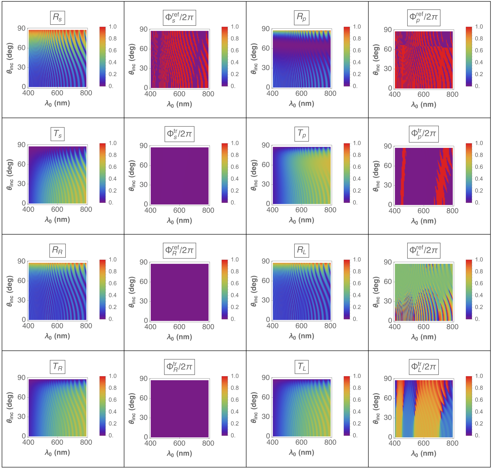
Figure 4: Spectrums of $R_{\ell}$, $T_{\ell}$, $\Phi^{\rm ref}_{\ell}$, and $\Phi^{\rm tr}_{\ell}$, $\ell\in\left\{s,p,R,L\right\}$, for $\theta_{\rm inc}\in[0^{\circ},90^{\circ})$, when $\tilde{N}=2$, $h=\pm 1$, $N=15$, $P=300$ nm, and $\psi=0^{\circ}$.

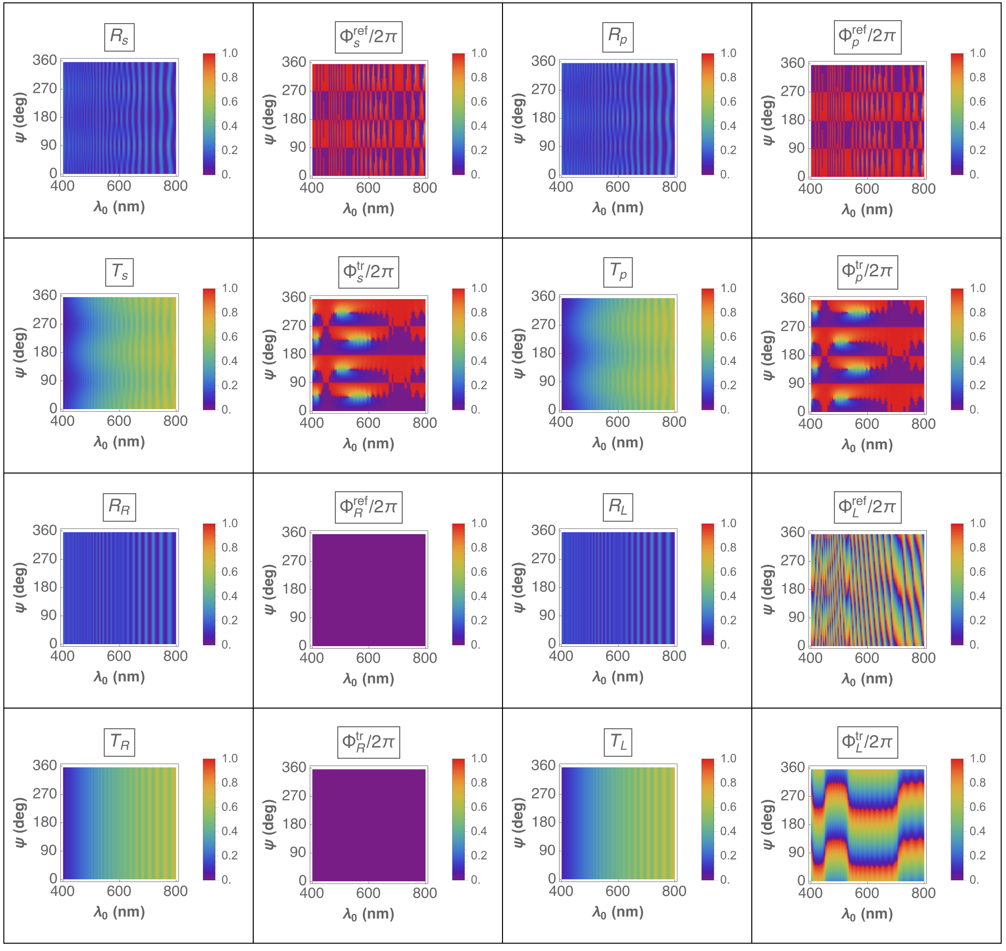
Figure 5: Spectrums of $R_{\ell}$, $T_{\ell}$, $\Phi^{\rm ref}_{\ell}$, and $\Phi^{\rm tr}_{\ell}$, $\ell\in\left\{s,p,R,L\right\}$, for $\psi\in[0^{\circ},360^{\circ})$, when $\tilde{N}=2$, $h=\pm 1$, $N=15$, $P=300$ nm, and $\theta_{\rm inc}=0^{\circ}$.

Figure 4 presents the spectrums of $R_{\ell}$, $T_{\ell}$, $\Phi^{\rm ref}_{\ell}$, and $\Phi^{\rm tr}_{\ell}$, $\ell\in\left\{s,p,R,L\right\}$, for $\theta_{\rm inc}\in[0^{\circ},90^{\circ})$ and $\psi=0^{\circ}$, and Fig. 5 for $\theta_{\rm inc}=0^{\circ}$ and $\psi\in[0^{\circ},360^{\circ})$. Neither the total remittances nor the corresponding geometric phases depend on whether $h=1$ or $h=-1$ in these two figures, just as in Figs. 2 and 3, because chevronic thin films lack structural handedness.

No trace of the Bragg phenomenon is evident in the plots of the total remittances in Figs. 4 and 5. There is no doubt that the Reusch pile is structurally periodic for $\tilde{N}=2$, but that structural periodicity does not translate into electromagnetic periodicity for all incidence conditions. Indeed for normal incidence, the interface $z=P/2$ in the reference unit cell is reflectionless [53, 54].

Elsewhere, theoretical research has shown that the Bragg phenomenon is not exhibited by a chevronic thin film for normal and near-normal incidence, which conclusion has been validated experimentally [42]. It is difficult to distinguish between the total remittance plots for $\tilde{N}=1$ (Figs. 2 and 3) and $\tilde{N}=2$ (Figs. 4 and 5). Theory also indicates vestigial manifestation of the Bragg phenomenon is possible for highly oblique incidence [42], but a clear signature cannot be discerned in Fig. 4.

The geometric phases $\Phi^{\rm ref}_{\ell}$ and $\Phi^{\rm tr}_{\ell}$, $\ell\in\left\{s,p,L\right\}$, are not identically zero in Figs. 4 and 5. Furthermore, although the total remittance plots in Fig. 2 are virtually indistinguishable from their counterparts in Fig. 4, the dependences of $\Phi^{\rm ref}_{\rm s,p}$, $\Phi^{\rm tr}_{\rm p}$, and $\Phi^{\rm ref}_{\rm L}$ on $\theta_{\rm inc}$ in those two figures show clear differences. These differences indicate that the geometric phases of the reflected and the transmitted plane waves are affected by morphology much more than the total remittances, this observation having been previously made only for the geometric phase of the transmitted plane wave [51, 52]. Note, however, that the plots of $\Phi^{\rm ref}_{\rm s,p}$, $\Phi^{\rm tr}_{\rm p}$, and $\Phi^{\rm ref}_{\rm L}$ in Figs. 3 and 5 are identical, because the interface $z=P/2$ in the middle of the reference unit cell of the chevronic thin film is electromagnetically inconsequential for normal incidence [53, 54].

3.3 Ambichiral Reusch pile ($\tilde{N}=3$)

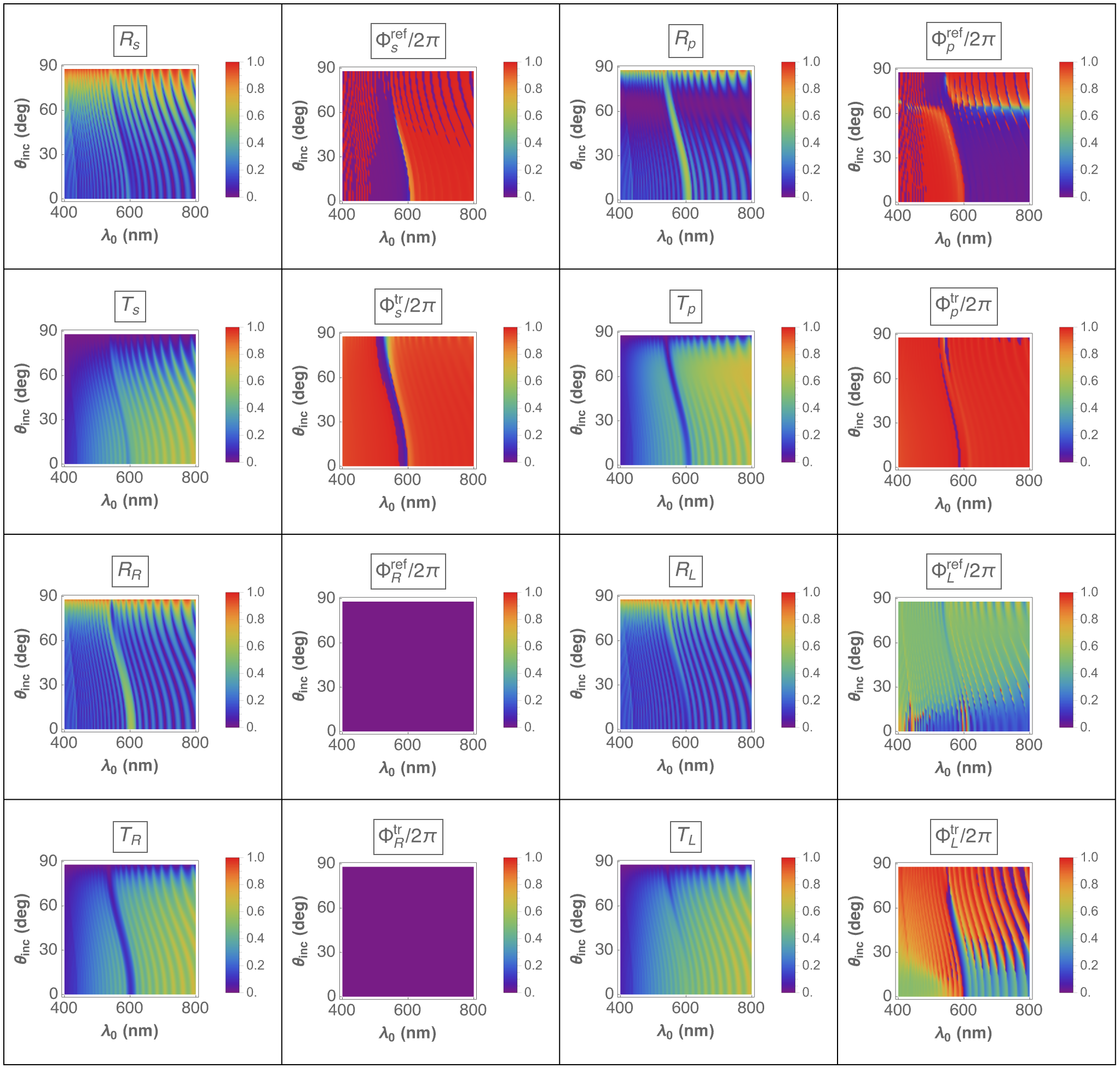
Figure 6: Spectrums of $R_{\ell}$, $T_{\ell}$, $\Phi^{\rm ref}_{\ell}$, and $\Phi^{\rm tr}_{\ell}$, $\ell\in\left\{s,p,R,L\right\}$, for $\theta_{\rm inc}\in[0^{\circ},90^{\circ})$, when $\tilde{N}=3$, $h=1$, $N=15$, $P=300$ nm, and $\psi=0^{\circ}$.

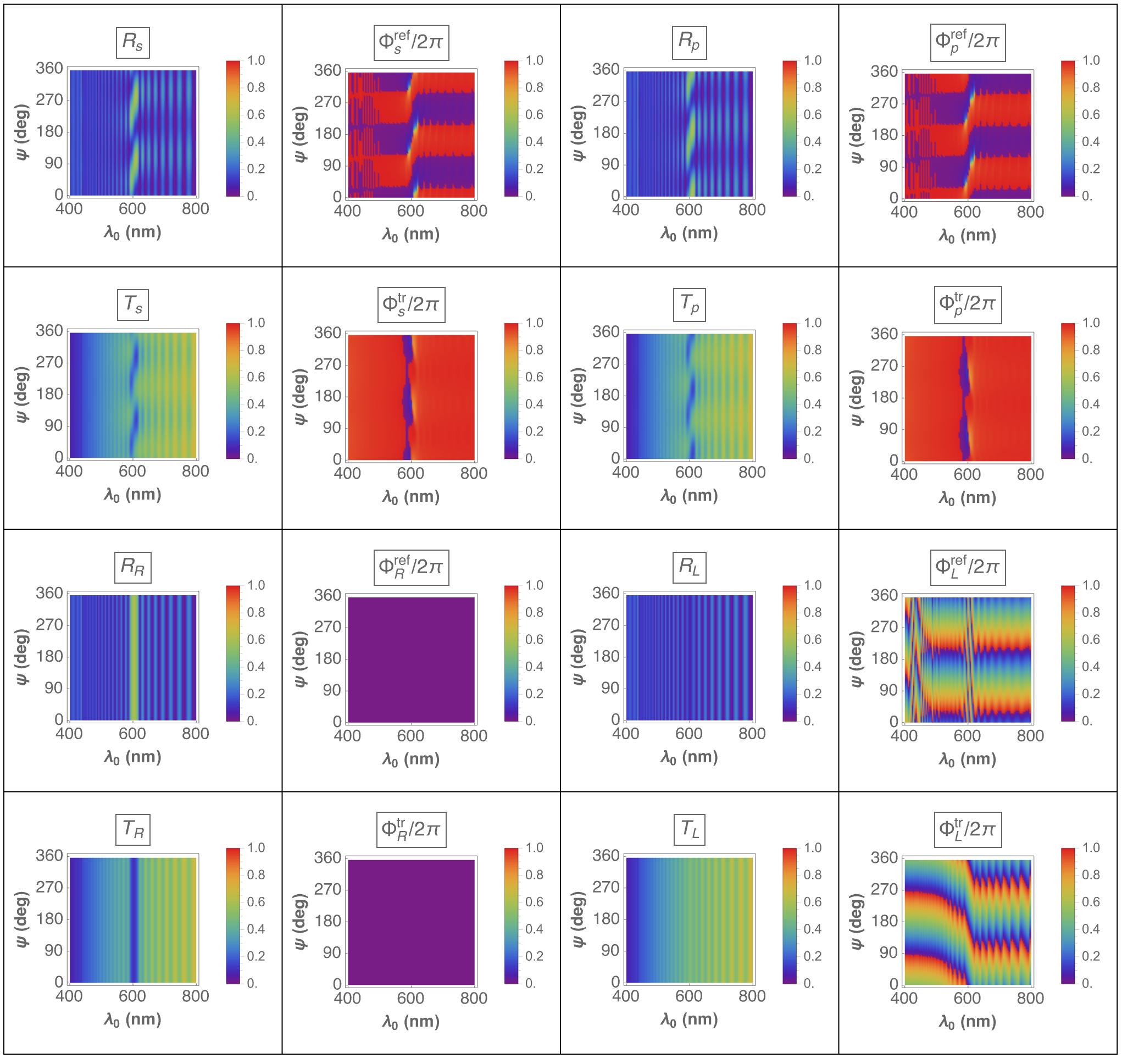
Figure 7: Spectrums of $R_{\ell}$, $T_{\ell}$, $\Phi^{\rm ref}_{\ell}$, and $\Phi^{\rm tr}_{\ell}$, $\ell\in\left\{s,p,R,L\right\}$, for $\psi\in[0^{\circ},360^{\circ})$, when $\tilde{N}=3$, $h=1$, $N=15$, $P=300$ nm, and $\theta_{\rm inc}=0^{\circ}$.

A Reusch pile with $\tilde{N}=3$ possesses both structural handedness and structural periodicity. Although this Reusch pile was not included in the 2004 classification [19], it should be considered as ambichiral. Figure 6 presents the chosen spectrums for $\theta_{\rm inc}\in[0^{\circ},90^{\circ})$ and $\psi=0^{\circ}$, and Fig. 7 for $\theta_{\rm inc}=0^{\circ}$ and $\psi\in[0^{\circ},360^{\circ})$, when $h=1$. The Bragg phenomenon is clearly evident as a deep blue trough in the plots of $T_{\rm R}$ and a corresponding ridge in the plots of $R_{\rm R}$. This trough/ridge is centered at $\lambda_{\scriptscriptstyle 0}=602$ nm for $\theta_{\rm inc}=0^{\circ}$ and it blueshifts with more oblique incidence [32]. The absence of analogous features in the plots of $T_{\rm L}$ and $R_{\rm L}$ supports the conclusion that this is a circular Bragg phenomenon. However, in comparison to a chiral sculptured thin film [32], the trough is present in the plots of both $T_{\rm R}$ and $T_{\rm L}$, and the ridge in the plots of both $R_{\rm R}$ and $R_{\rm L}$, for highly oblique incidence.

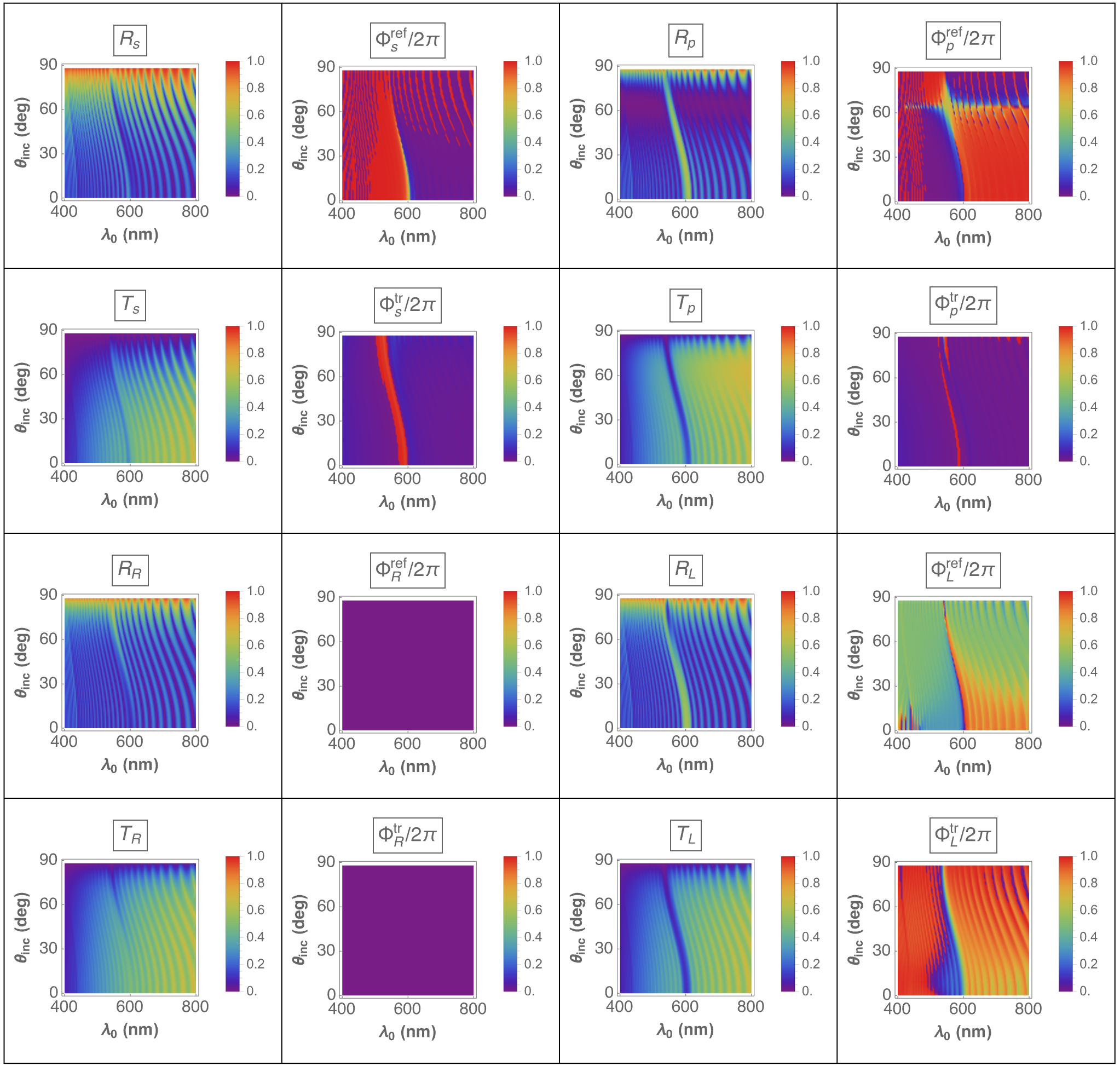
Figure 8: Spectrums of $R_{\ell}$, $T_{\ell}$, $\Phi^{\rm ref}_{\ell}$, and $\Phi^{\rm tr}_{\ell}$, $\ell\in\left\{s,p,R,L\right\}$, for $\theta_{\rm inc}\in[0^{\circ},90^{\circ})$, when $\tilde{N}=3$, $h=-1$, $N=15$, $P=300$ nm, and $\psi=0^{\circ}$.

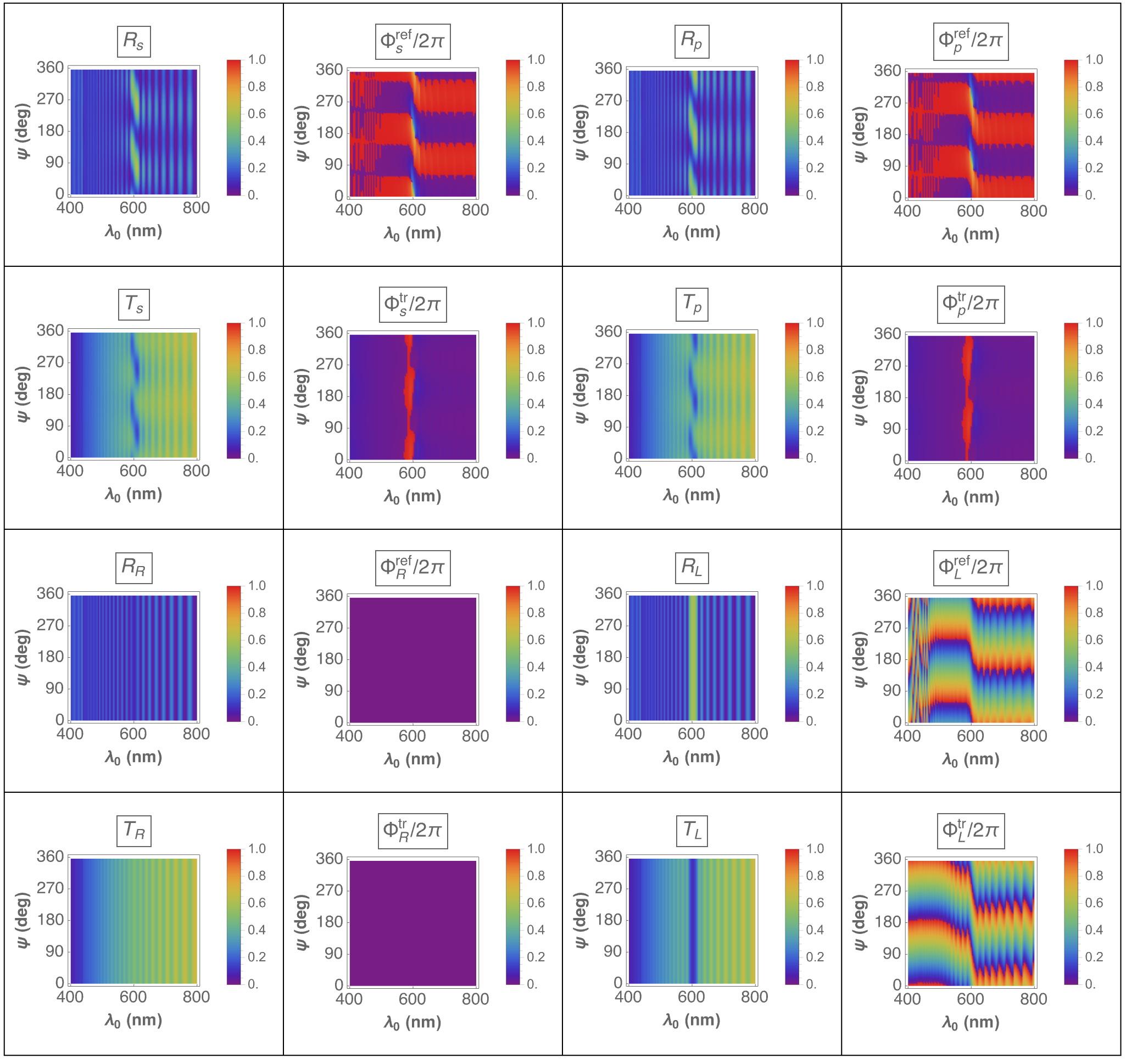
Figure 9: Spectrums of $R_{\ell}$, $T_{\ell}$, $\Phi^{\rm ref}_{\ell}$, and $\Phi^{\rm tr}_{\ell}$, $\ell\in\left\{s,p,R,L\right\}$, for $\psi\in[0^{\circ},360^{\circ})$, when $\tilde{N}=3$, $h=-1$, $N=15$, $P=300$ nm, and $\theta_{\rm inc}=0^{\circ}$.

Analogous spectrums for $h=-1$ are presented in Figs. 8 and 9. The plots of $\left\{T_{\rm R},R_{\rm R},T_{\rm L},R_{\rm L}\right\}$ for fixed $\psi$ are interchanged with those of $\left\{T_{\rm L},R_{\rm L},T_{\rm R},R_{\rm R}\right\}$ for $2\pi-\psi$, in comparison to Figs. 6 and 7; in other words,

$$\left.\begin{array}[]{ll}R_{\rm R}(h,\psi)=R_{\rm L}(-h,2\pi-\psi)\,,&R_{\rm L}(h,\psi)=R_{\rm R}(-h,2\pi-\psi)\\[5.0pt] T_{\rm R}(h,\psi)=T_{\rm L}(-h,2\pi-\psi)\,,&T_{\rm L}(h,\psi)=T_{\rm R}(-h,2\pi-\psi)\end{array}\right\}\,.$$ (23)

Since a linearly polarized plane wave can be decomposed into an RCP plane wave and an LCP plane wave, signatures of the circular Bragg phenomenon are also to be found in the plots of linear remittances in Figs. 6–9. The following symmetries are exhibited by the linear remittances:

$$\left.\begin{array}[]{ll}R_{\rm s}(h,\psi)=R_{\rm s}(-h,2\pi-\psi)\,,&R_{\rm p}(h,\psi)=R_{\rm p}(-h,2\pi-\psi)\\[5.0pt] T_{\rm s}(h,\psi)=T_{\rm s}(-h,2\pi-\psi)\,,&T_{\rm p}(h,\psi)=T_{\rm p}(-h,2\pi-\psi)\end{array}\right\}\,.$$ (24)

No symmetries are evident in the plots of geometric phases in Figs. 6–9, except that $\Phi_{\rm R}^{\rm ref}=\Phi_{\rm R}^{\rm tr}\equiv 0$ by virtue of the structure of the Poincaré spinor of a RCP plane wave [51, 52]. The spectrums of $\Phi_{\ell}^{\rm ref}$ and $\Phi_{\ell}^{\rm tr}$, $\ell\in\left\{s,p,L\right\}$, are greatly affected when the structural handedness is reversed.

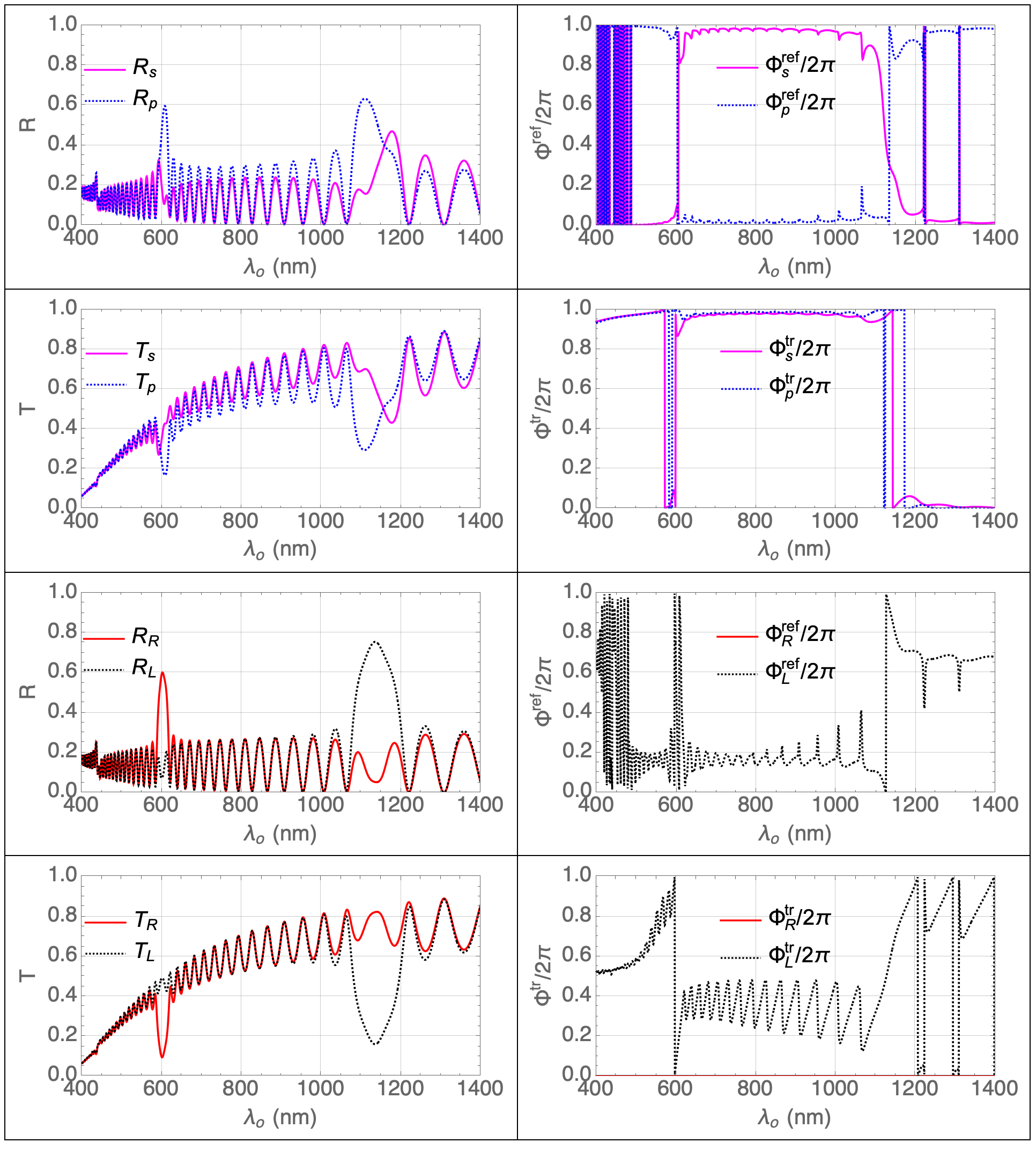
Figure 10: Spectrums of $R_{\ell}$, $T_{\ell}$, $\Phi^{\rm ref}_{\ell}$, and $\Phi^{\rm tr}_{\ell}$, $\ell\in\left\{s,p,R,L\right\}$, for $\theta_{\rm inc}=0^{\circ}$ and $\psi=0^{\circ}$, when $\tilde{N}=3$, $h=1$, $N=15$, and $P=300$ nm.

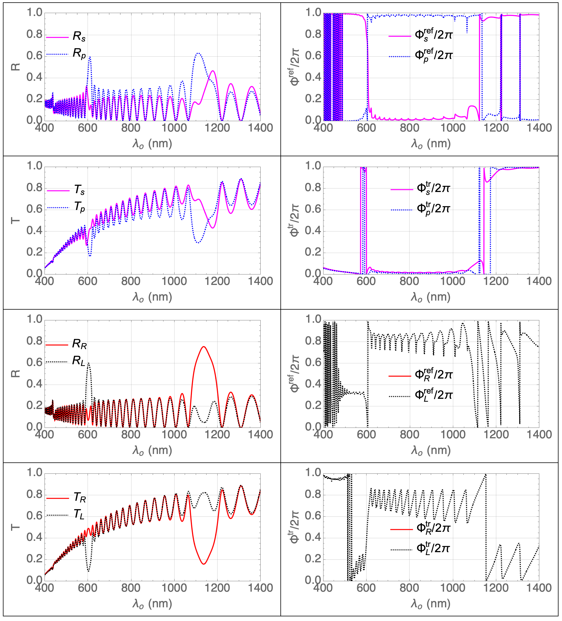
Figure 11: Spectrums of $R_{\ell}$, $T_{\ell}$, $\Phi^{\rm ref}_{\ell}$, and $\Phi^{\rm tr}_{\ell}$, $\ell\in\left\{s,p,R,L\right\}$, for $\theta_{\rm inc}=0^{\circ}$ and $\psi=0^{\circ}$, when $\tilde{N}=3$, $h=-1$, $N=15$, and $P=300$ nm.

In order to confirm that $\tilde{N}=3$ provides the exceptional case $\lambda_{\scriptscriptstyle 0}^{2;0,\tilde{N}/2}>\lambda_{\scriptscriptstyle 0}^{1;0,\tilde{N}/2}$, calculations were also made for $\lambda_{\scriptscriptstyle 0}$ extending into the near-infrared spectral regime. With $\theta_{\rm inc}=0^{\circ}$ and $\psi=0^{\circ}$ fixed, (i) Fig. 10 presents the spectrums of $R_{\ell}$, $T_{\ell}$, $\Phi^{\rm ref}_{\ell}$, and $\Phi^{\rm tr}_{\ell}$, $\ell\in\left\{s,p,R,L\right\}$, for $h=1$, and Fig. 11 presents the same spectrums for $h=-1$. The remittance spectrums in both figures clearly show two circular Bragg regimes. The first is centered at $\lambda_{\scriptscriptstyle 0}^{1;0,3/2}=602$ nm, exactly as in Figs. 6–9, and it belongs to the first family described in Sec. 1.3. The second is centered at $\lambda_{\scriptscriptstyle 0}^{2;0,3/2}=1135$ nm and belongs to the second family described in Sec. 1.3. Note that $\lambda_{\scriptscriptstyle 0}^{2;0,3/2}$ differs from $2\lambda_{\scriptscriptstyle 0}^{1;0,3/2}$ predicted by Eq. (9) because the relative permittivity scalars in Eq. (22) are frequency dependent.

Importantly, the spectral variations of $\Phi^{\rm ref}_{\ell}$ and $\Phi^{\rm tr}_{\ell}$, $\ell\in\left\{s,p,L\right\}$, are different in the two circular Bragg regimes in Figs. 10 and 11.

3.4 Equichiral Reusch pile ($\tilde{N}=4$)

The prefix equi in the classification equichiral is justified for a Reusch pile with $\tilde{N}=4$, since $\lambda_{\scriptscriptstyle 0}^{1;p,\tilde{N}/2}=\lambda_{\scriptscriptstyle 0}^{2;p,\tilde{N}/2}$ $\forall{p}$ when $\tilde{N}=4$. The same Reusch pile is also structurally handed (with period $P$), so that the suffix chiral in the classification equichiral is also justified. However, there is a notable exception: the period equals $P/2$ and there is no structural handedness when $\chi\in\left\{0,\pi/2\right\}$.

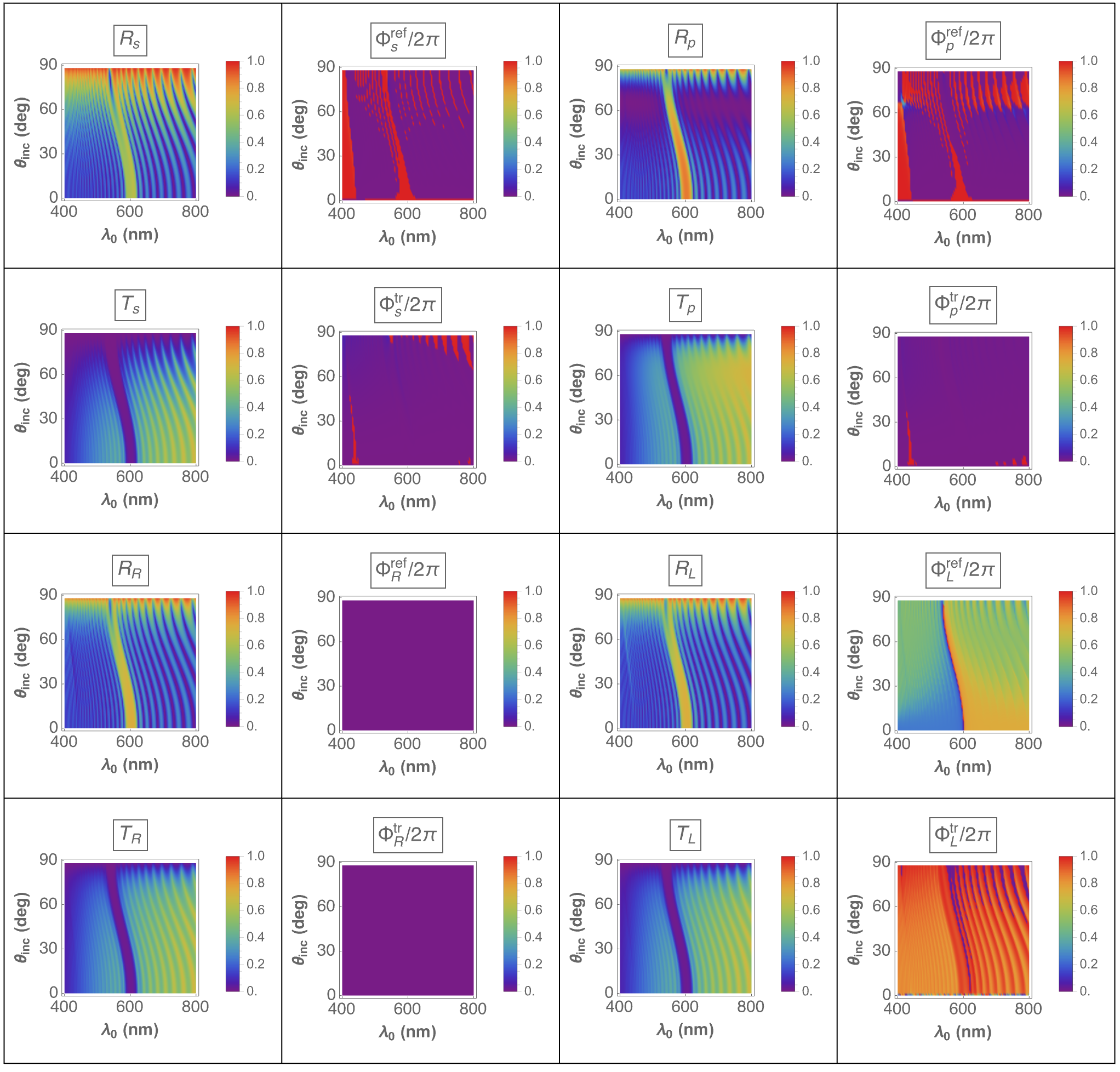
Figure 12: Spectrums of $R_{\ell}$, $T_{\ell}$, $\Phi^{\rm ref}_{\ell}$, and $\Phi^{\rm tr}_{\ell}$, $\ell\in\left\{s,p,R,L\right\}$, for $\theta_{\rm inc}\in[0^{\circ},90^{\circ})$, when $\tilde{N}=4$, $h=1$, $N=15$, $P=300$ nm, and $\psi=0^{\circ}$.

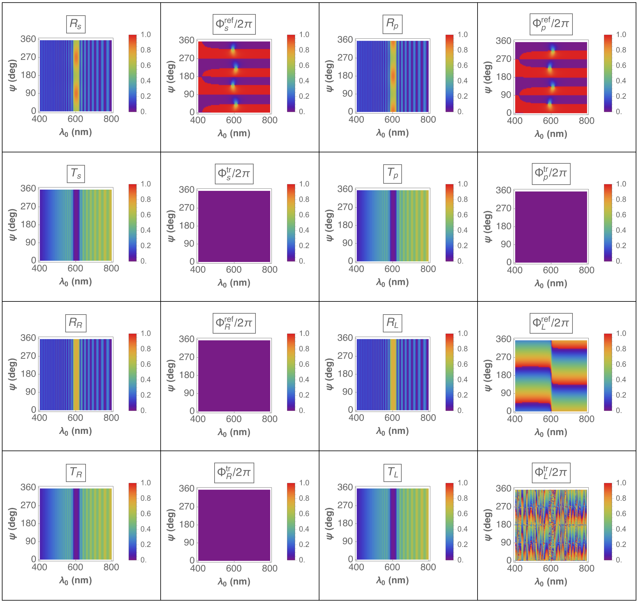
Figure 13: Spectrums of $R_{\ell}$, $T_{\ell}$, $\Phi^{\rm ref}_{\ell}$, and $\Phi^{\rm tr}_{\ell}$, $\ell\in\left\{s,p,R,L\right\}$, for $\psi\in[0^{\circ},360^{\circ})$, when $\tilde{N}=4$, $h=1$, $N=15$, $P=300$ nm, and $\theta_{\rm inc}=0^{\circ}$.

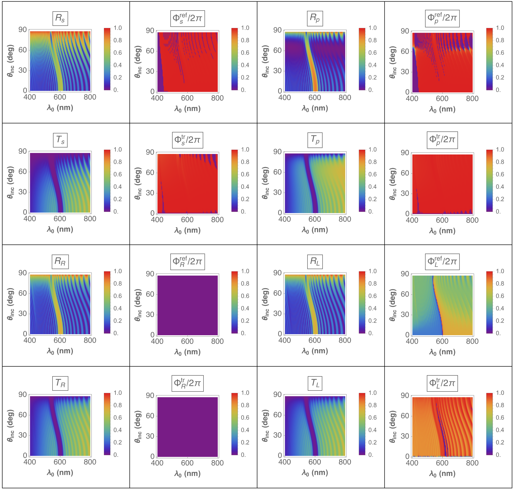
Figure 14: Spectrums of $R_{\ell}$, $T_{\ell}$, $\Phi^{\rm ref}_{\ell}$, and $\Phi^{\rm tr}_{\ell}$, $\ell\in\left\{s,p,R,L\right\}$, for $\theta_{\rm inc}\in[0^{\circ},90^{\circ})$, when $\tilde{N}=4$, $h=-1$, $N=15$, $P=300$ nm, and $\psi=0^{\circ}$.

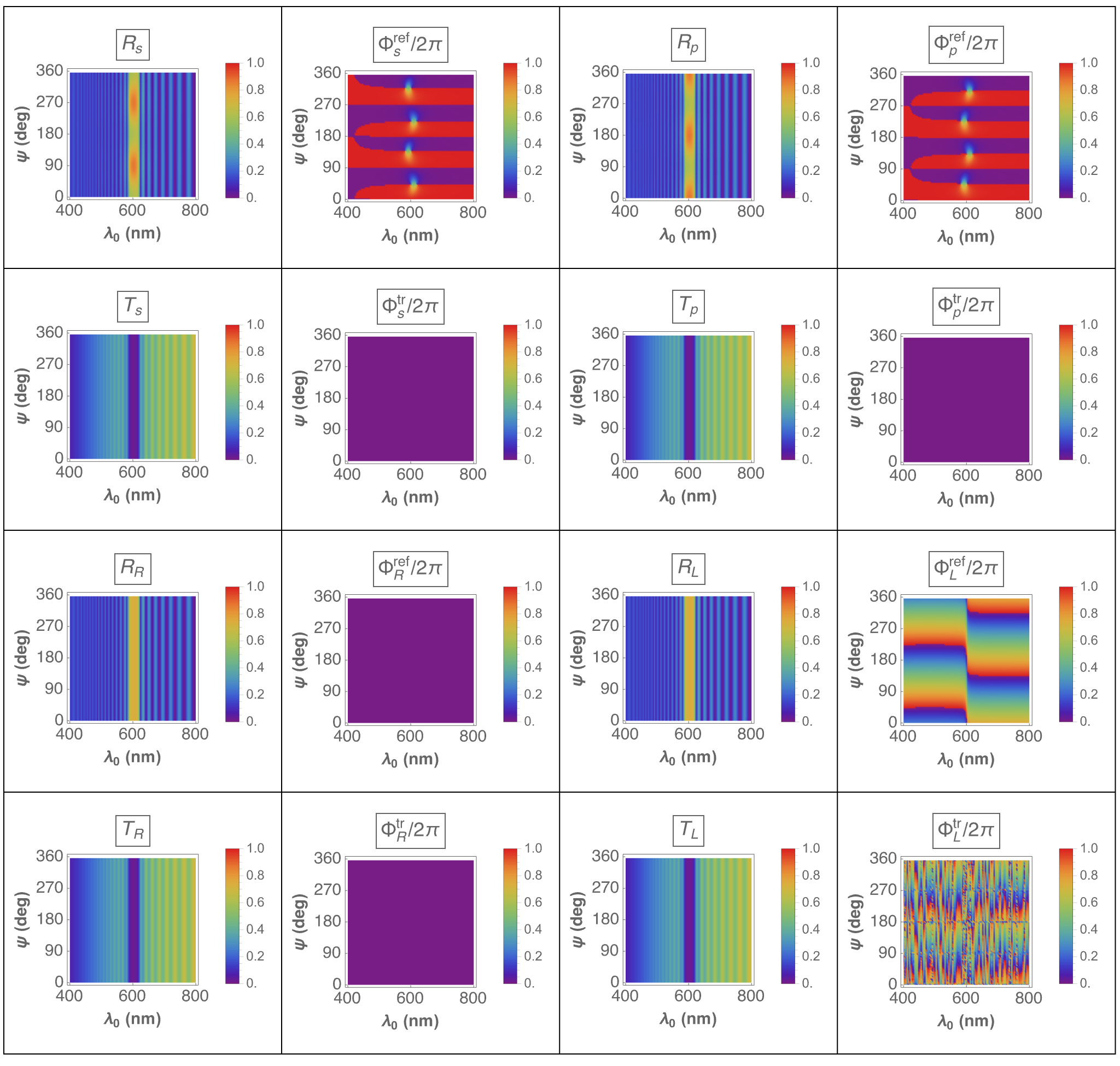
Figure 15: Spectrums of $R_{\ell}$, $T_{\ell}$, $\Phi^{\rm ref}_{\ell}$, and $\Phi^{\rm tr}_{\ell}$, $\ell\in\left\{s,p,R,L\right\}$, for $\psi\in[0^{\circ},360^{\circ})$, when $\tilde{N}=4$, $h=-1$, $N=15$, $P=300$ nm, and $\theta_{\rm inc}=0^{\circ}$.

Figure 12 presents the chosen spectrums for $\theta_{\rm inc}\in[0^{\circ},90^{\circ})$ and $\psi=0^{\circ}$, and Fig. 13 for $\theta_{\rm inc}=0^{\circ}$ and $\psi\in[0^{\circ},360^{\circ})$, when $h=1$. Figures 14 and 15 are the counterparts of those two figures for $h=-1$. Calculations show that Eqs. (23) and (24) hold for $\tilde{N}=4$.

The Bragg phenomenon is clearly evident as a deep blue trough in the plots of both linear and both circular transmittances, and as a corresponding ridge in the plots of both linear and both circular reflectances, regardless of the value of $h\in\left\{-1,1\right\}$. These features are centered about $\lambda_{\scriptscriptstyle 0}=600$ nm for $\theta_{\rm inc}=0^{\circ}$ and blueshift with more oblique incidence. This Reusch pile exhibits a polarization-universal bandgap that can be tuned by adjusting the angle of incidence $\theta_{\rm inc}$, as has been verified experimentally [35].

The plots of $\Phi_{\ell}^{\rm ref}$ and $\Phi_{\ell}^{\rm tr}$, $\ell\in\left\{s,p,L\right\}$, in general, contain clear evidence of the polarization-universal bandgap. However, whereas $\Phi_{\ell}^{\rm ref}$ and $\Phi_{\ell}^{\rm tr}$, $\ell\in\left\{s,p\right\}$, are greatly affected when the structural handedness is reversed, $\Phi_{L}^{\rm ref}$ and $\Phi_{L}^{\rm tr}$ are affected very little by the same reversal.

3.5 Ambichiral and finely chiral Reusch piles ($\tilde{N}\geq 5$)

The optical response characteristics for $\tilde{N}\geq 5$ are similar to those for $\tilde{N}=3$, except that Eq. (9) predicts $\lambda_{\scriptscriptstyle 0}^{2;0,\tilde{N}/2}/\lambda_{\scriptscriptstyle 0}^{1;0,\tilde{N}/2}>1$ for $\tilde{N}=3$ but $\lambda_{\scriptscriptstyle 0}^{2;0,\tilde{N}/2}/\lambda_{\scriptscriptstyle 0}^{1;0,\tilde{N}/2}<1$ for $\tilde{N}\geq 5$.

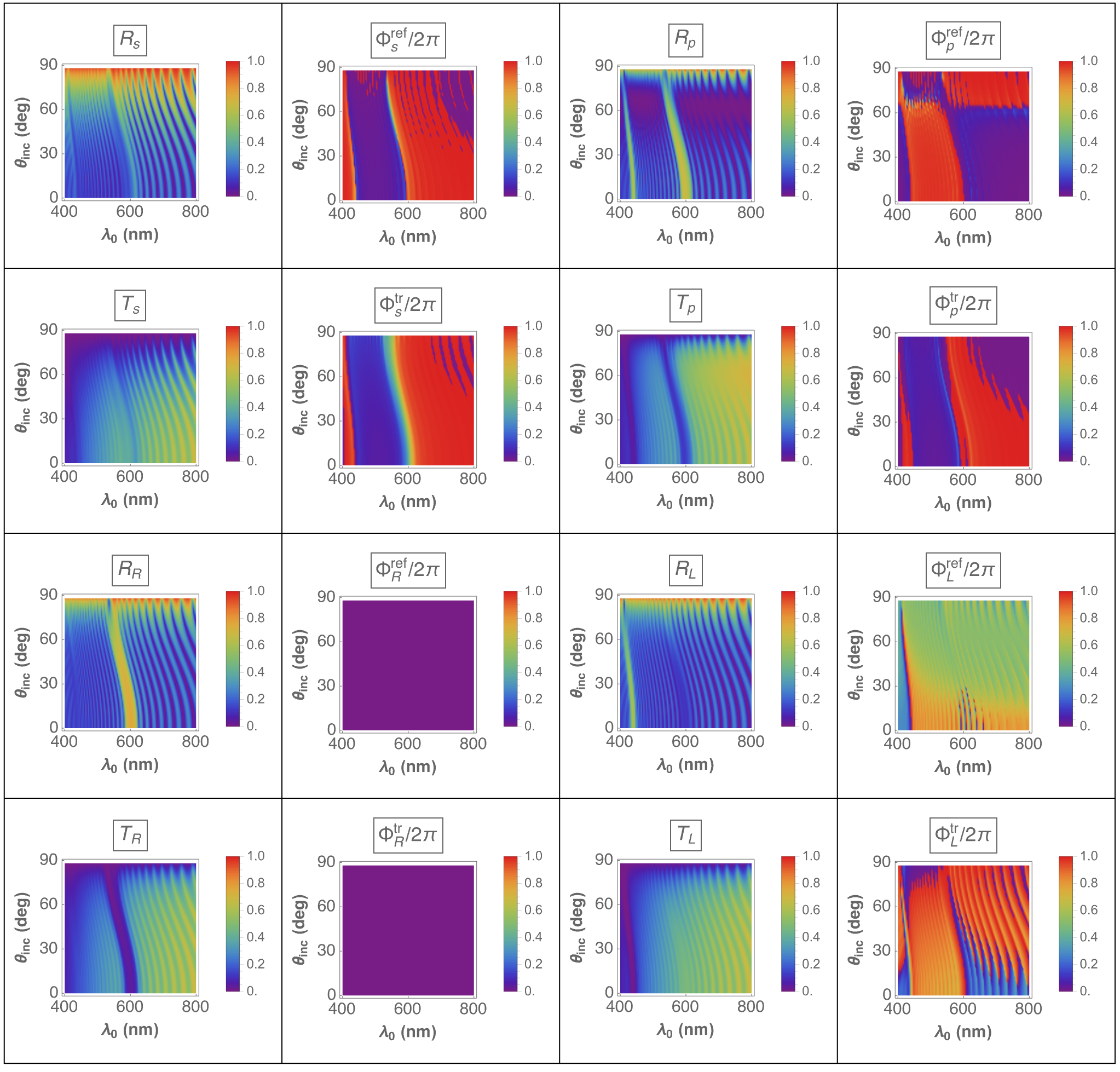
Figure 16: Spectrums of $R_{\ell}$, $T_{\ell}$, $\Phi^{\rm ref}_{\ell}$, and $\Phi^{\rm tr}_{\ell}$, $\ell\in\left\{s,p,R,L\right\}$, for $\theta_{\rm inc}\in[0^{\circ},90^{\circ})$, when $\tilde{N}=5$, $h=1$, $N=15$, $P=300$ nm, and $\psi=0^{\circ}$.

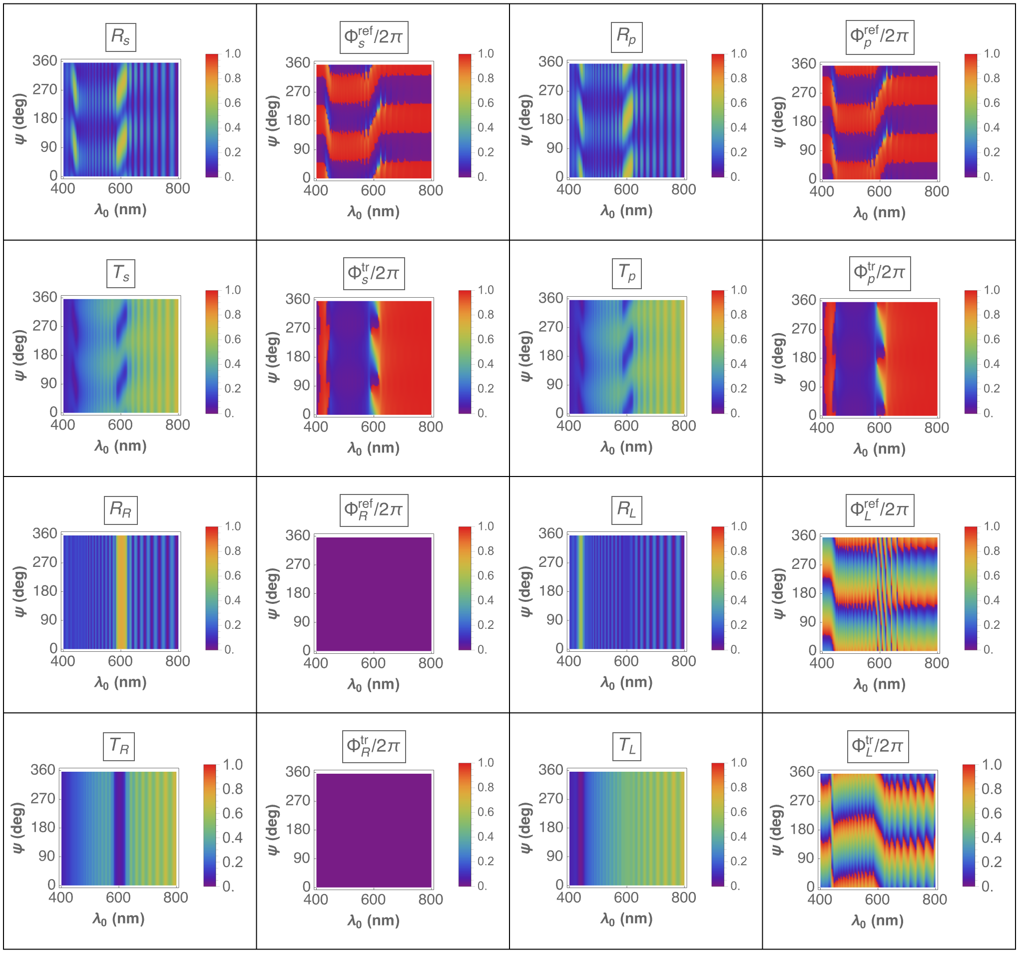
Figure 17: Spectrums of $R_{\ell}$, $T_{\ell}$, $\Phi^{\rm ref}_{\ell}$, and $\Phi^{\rm tr}_{\ell}$, $\ell\in\left\{s,p,R,L\right\}$, for $\psi\in[0^{\circ},360^{\circ})$, when $\tilde{N}=5$, $h=1$, $N=15$, $P=300$ nm, and $\theta_{\rm inc}=0^{\circ}$.

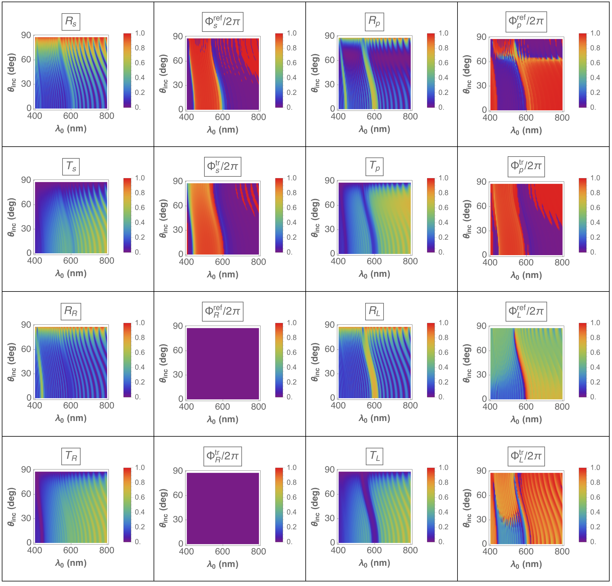
Figure 18: Spectrums of $R_{\ell}$, $T_{\ell}$, $\Phi^{\rm ref}_{\ell}$, and $\Phi^{\rm tr}_{\ell}$, $\ell\in\left\{s,p,R,L\right\}$, for $\theta_{\rm inc}\in[0^{\circ},90^{\circ})$, when $\tilde{N}=5$, $h=-1$, $N=15$, $P=300$ nm, and $\psi=0^{\circ}$.

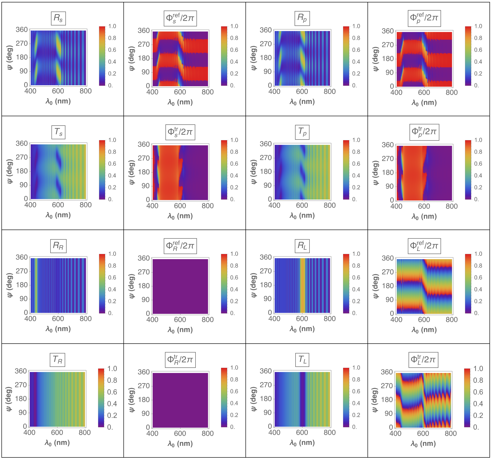
Figure 19: Spectrums of $R_{\ell}$, $T_{\ell}$, $\Phi^{\rm ref}_{\ell}$, and $\Phi^{\rm tr}_{\ell}$, $\ell\in\left\{s,p,R,L\right\}$, for $\psi\in[0^{\circ},360^{\circ})$, when $\tilde{N}=5$, $h=-1$, $N=15$, $P=300$ nm, and $\theta_{\rm inc}=0^{\circ}$.

Figure 16 presents the chosen spectrums for $\theta_{\rm inc}\in[0^{\circ},90^{\circ})$ and $\psi=0^{\circ}$, and Fig. 17 for $\theta_{\rm inc}=0^{\circ}$ and $\psi\in[0^{\circ},360^{\circ})$, when $\tilde{N}=5$ and $h=1$. Analogous spectrums for $\tilde{N}=5$ and $h=-1$ are presented in Figs. 18 and 19. Regardless of whether $h=1$ or $h=-1$, two distinct circular Bragg regimes are evident in these plots. Whereas $\lambda_{\scriptscriptstyle 0}^{1;0,5/2}=602$ nm for $\theta_{\rm inc}=0^{\circ}$, we have $\lambda_{\scriptscriptstyle 0}^{2;0,5/2}=439$ nm for normal incidence, so that $\lambda_{\scriptscriptstyle 0}^{2;0,5/2}/\lambda_{\scriptscriptstyle 0}^{1;0,5/2}=0.729$. This ratio is smaller than $0.667$ predicted by Eq. (9), because the relative permittivity scalars in Eq. (22) are frequency dependent.

Equations (23) and (24) hold, but similar symmetries are not evident for the non-zero geometric phases in Figs. 16–19. Furthermore, the spectral variations of $\Phi^{\rm ref}_{\ell}$ and $\Phi^{\rm tr}_{\ell}$, $\ell\in\left\{s,p,L\right\}$, are different in the two circular Bragg regimes in these figures.

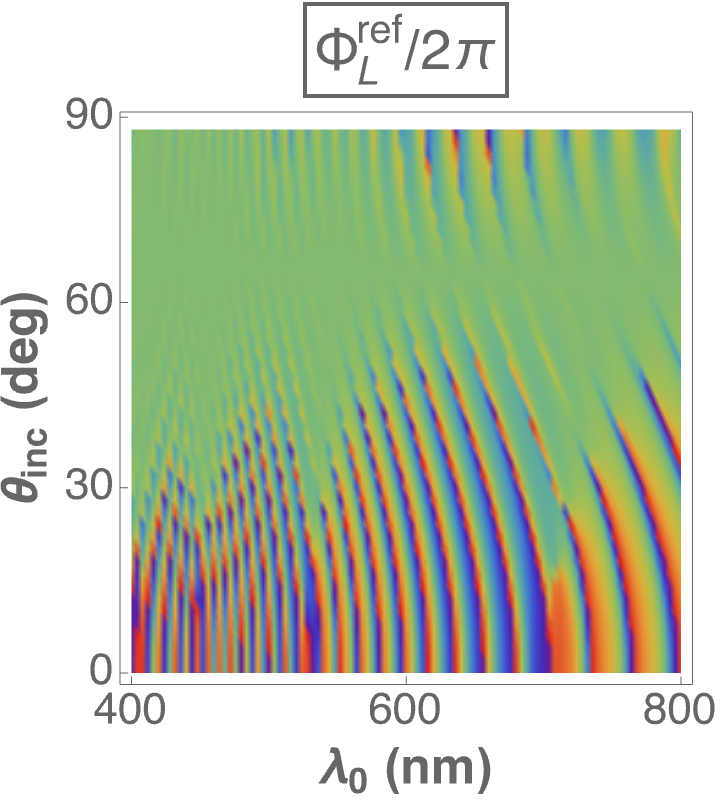
(b) $\tilde{N}=2$

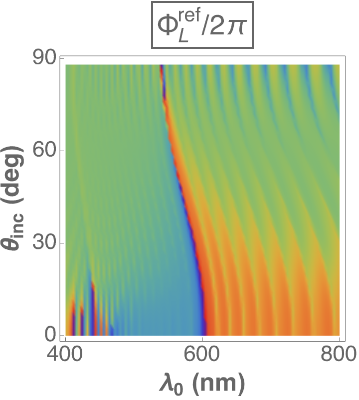
(c) $\tilde{N}=3$

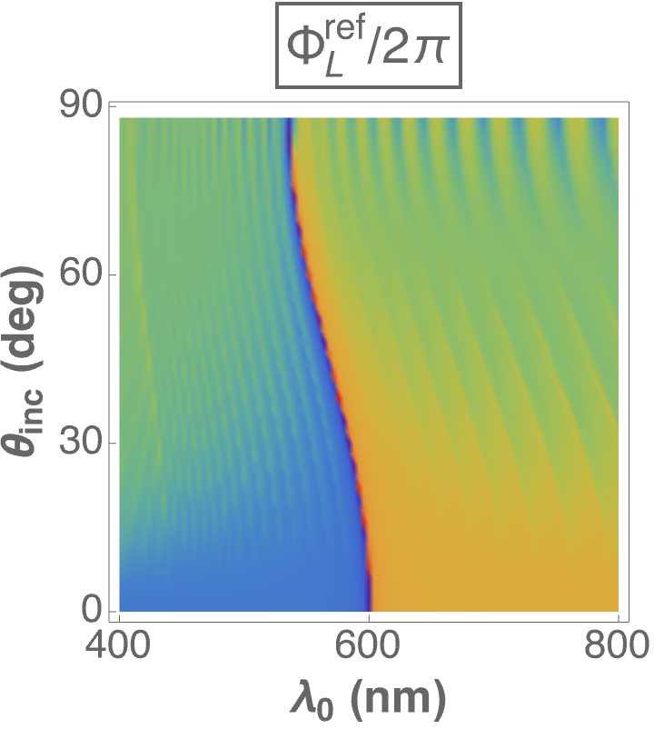
(d) $\tilde{N}=4$

(e) $\tilde{N}=5$

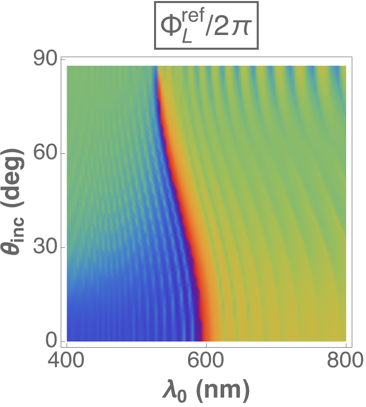
(f) $\tilde{N}=6$

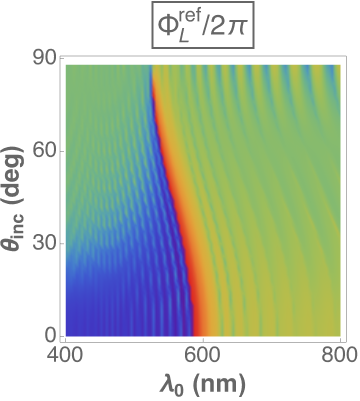
(g) $\tilde{N}=8$

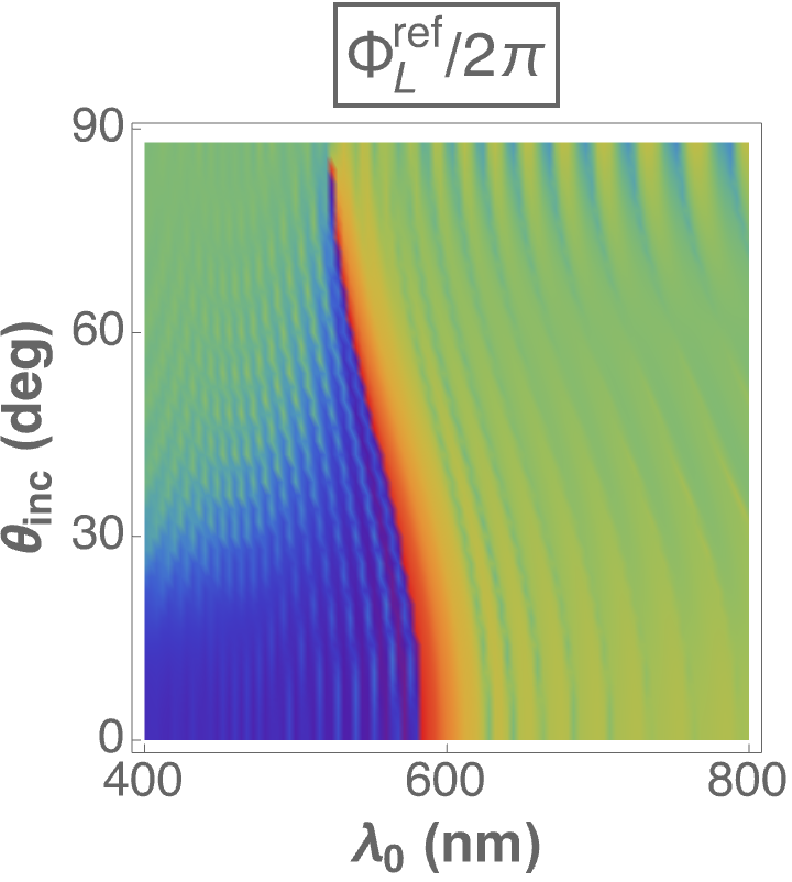
(h) $\tilde{N}=10$

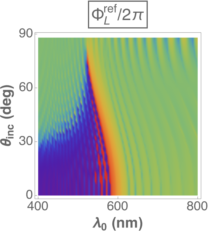
(i) $\tilde{N}=20$

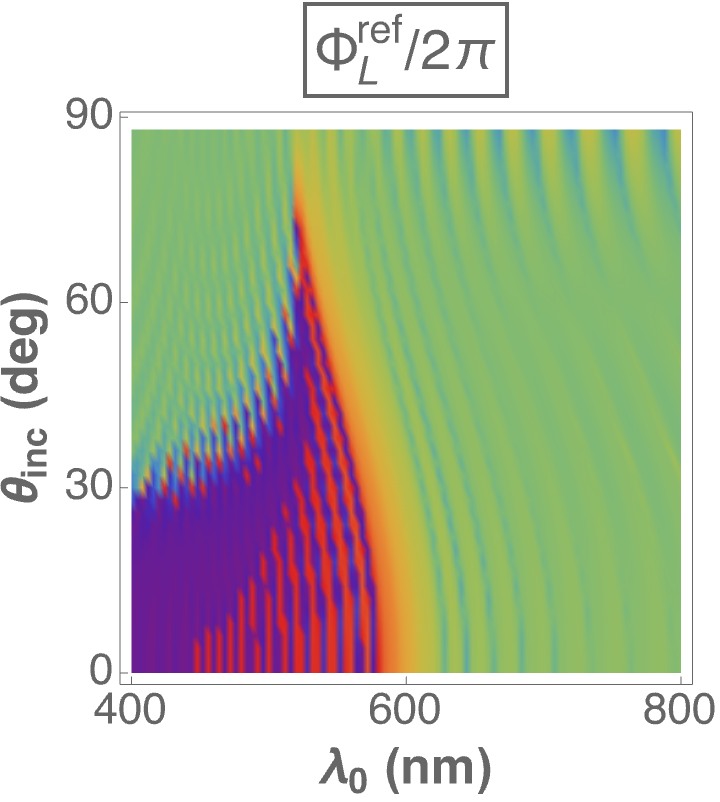
(j) $\tilde{N}=50$

Figure 21: Spectrums of $\Phi^{\rm ref}_{L}$ for $\theta_{\rm inc}\in[0^{\circ},90^{\circ})$ and $\tilde{N}\in\left\{1,2,3,4,5,6,8,10,20,50\right\}$, when $h=-1$, $N=15$, $P=300$ nm, and $\psi=0^{\circ}$.

The Reusch pile becomes finely chiral and $\lambda_{\scriptscriptstyle 0}^{2;0,\tilde{N}/2}$ blueshifts ever farther from $\lambda_{\scriptscriptstyle 0}^{1;0,\tilde{N}/2}$, as $\tilde{N}$ increases significantly beyond $5$, and the circular total remittance spectrums begin to converge [39]. A similar convergence is also exhibited by the linear total remittance spectrums. Spectrums of the non-zero geometric phases also appear to converge, except in the vicinity of a circular Bragg regime. This becomes clear from examining the plots of $\Phi_{\rm L}^{\rm tr}$ for $\psi=0^{\circ}$, $h=1$ and $\tilde{N}\in[1,50]$ in Fig. (20), wherein the choice of $\Phi_{\rm L}^{\rm tr}$ over other non-zero geometric phases takes into account the fact that $T_{\rm L}$ is high inside the circular Bragg regime with $\lambda_{\scriptscriptstyle 0}^{1;0,\tilde{N}/2}$ as its center wavelength for $h=1$. The same conclusion emerges even more strongly from examining the plots of $\Phi_{\rm L}^{\rm ref}$ for $\psi=0^{\circ}$, $h=-1$, and $\tilde{N}\in[1,50]$ in Fig. (21), the choice of $\Phi_{\rm L}^{\rm ref}$ over other non-zero geometric phases taking into account that $R_{\rm L}$ is high inside the circular Bragg regime with $\lambda_{\scriptscriptstyle 0}^{1;0,\tilde{N}/2}$ as its center wavelength for $h=-1$.

4 Concluding remarks

Figures (2)–(19) provide an evolutionary perspective on the nanoscale architected morphology of Reusch piles. Total remittances and geometric phases were presented as functions of the free-space wavelength and the direction of plane-wave incidence for fixed thickness $NP=4500$ nm with $N=15$. As $\tilde{N}$ increased from unity, first the Reusch pile became structurally periodic (for $\tilde{N}\geq 2$) and then structurally handed (for $\tilde{N}\geq 3$). The layer thickness $P/\tilde{N}$ continued to shrink with increasing $\tilde{N}$, which can be implemented quite straightforwardly with chiral sculptured thin films [19, 36]. Total-remittance values in excess of $0.01$ began to converge correct to four decimal digits, as $\tilde{N}$ increased beyond $10$ (results not shown).

But that did not turn out to be completely true for the geometric phases. With $\Phi_{\rm L}^{\rm tr}$ selected for $h=1$ because $T_{\rm L}$ has a substantial magnitude inside the circular Bragg regime with $\lambda_{\scriptscriptstyle 0}^{1;0,\tilde{N}/2}$ as its center wavelength, and $\Phi_{\rm L}^{\rm ref}$ selected for $h=-1$ because $R_{\rm L}$ has a substantial magnitude inside the same circular Bragg regime, to facilitate measurements eventually, Figs. (20) and (21) show the emergence of new features in the spectrums of non-zero geometric phases on the short-wavelength side of the chosen circular Bragg regime. Since adjacent layers in a Reusch pile with high $\tilde{N}$ are, at least theoretically identical except for a slight twist about the $z$ axis, the foregoing observation implies that the geometric phases are sensitive to nanoscale morphological changes as a thin film grows. Therefore, geometric phases could contain signatures of nanoscale morphological details that would depend on the fabrication technique. Careful experiments are necessary to establish this possibility.

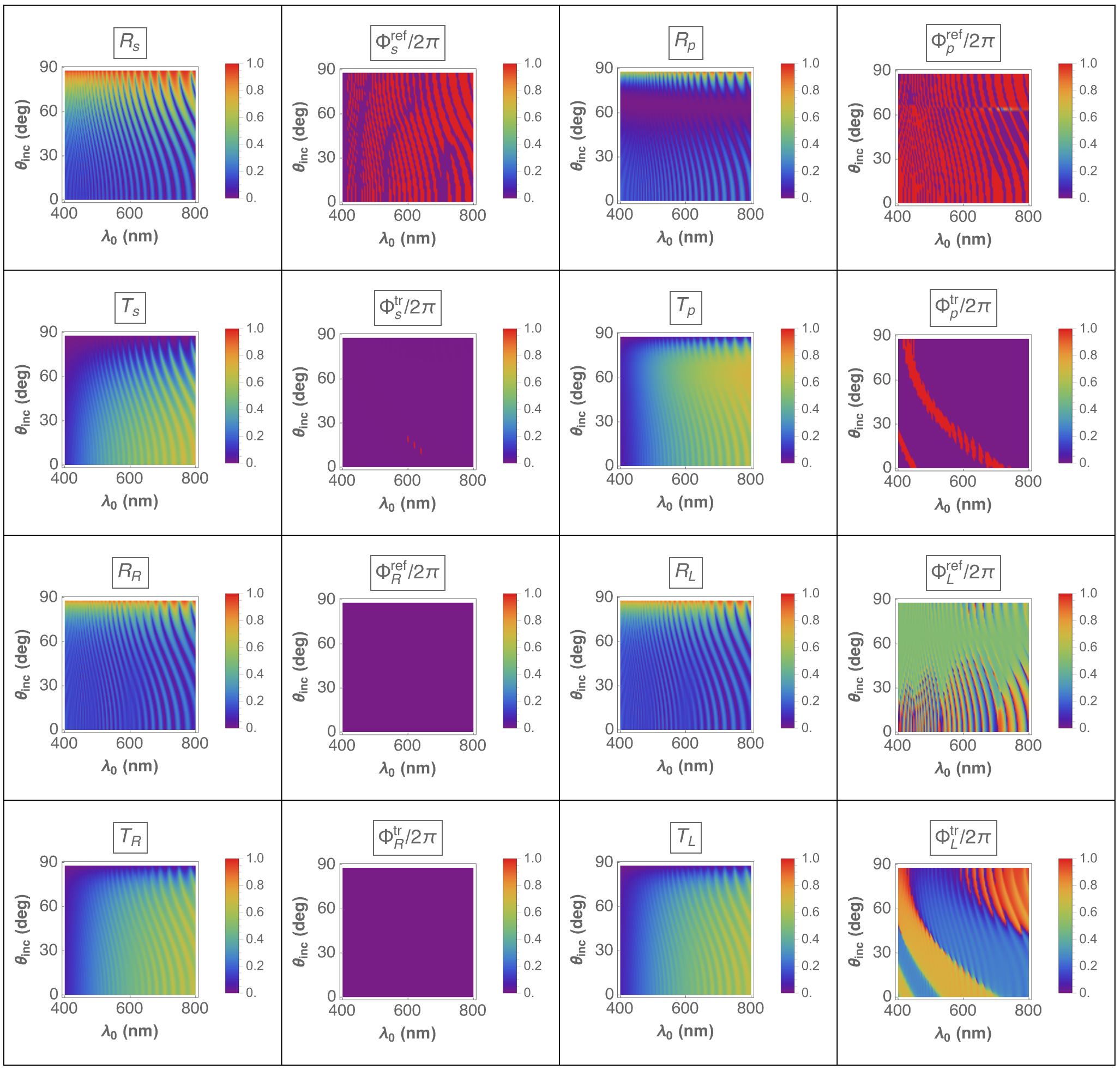
Figure 2: Spectrums of $R_{\ell}$, $T_{\ell}$, $\Phi^{\rm ref}_{\ell}$, and $\Phi^{\rm tr}_{\ell}$, $\ell\in\left\{s,p,R,L\right\}$, for $\theta_{\rm inc}\in[0^{\circ},90^{\circ})$, when $\tilde{N}=1$, $h=\pm 1$, $N=15$, $P=300$ nm, and $\psi=0^{\circ}$.

Figure 3: Spectrums of $R_{\ell}$, $T_{\ell}$, $\Phi^{\rm ref}_{\ell}$, and $\Phi^{\rm tr}_{\ell}$, $\ell\in\left\{s,p,R,L\right\}$, for $\psi\in[0^{\circ},360^{\circ})$, when $\tilde{N}=1$, $h=\pm 1$, $N=15$, $P=300$ nm, and $\theta_{\rm inc}=0^{\circ}$.

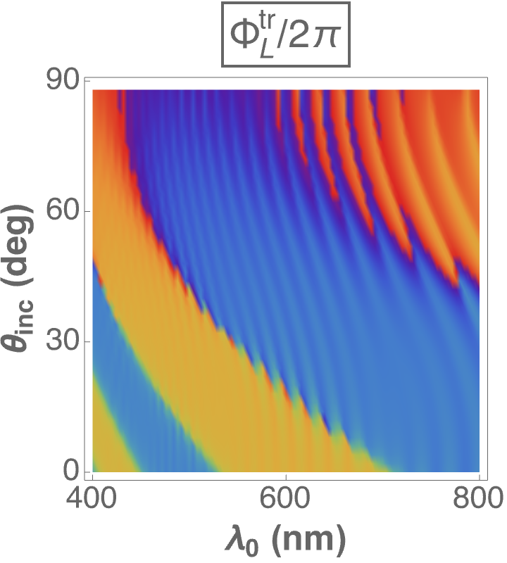
(a) $\tilde{N}=1$

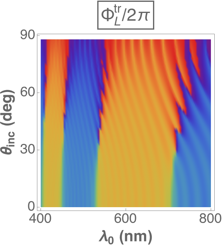
(b) $\tilde{N}=2$

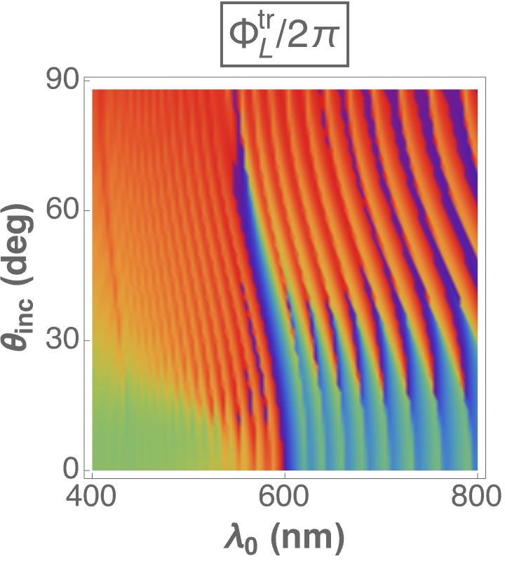
(c) $\tilde{N}=3$

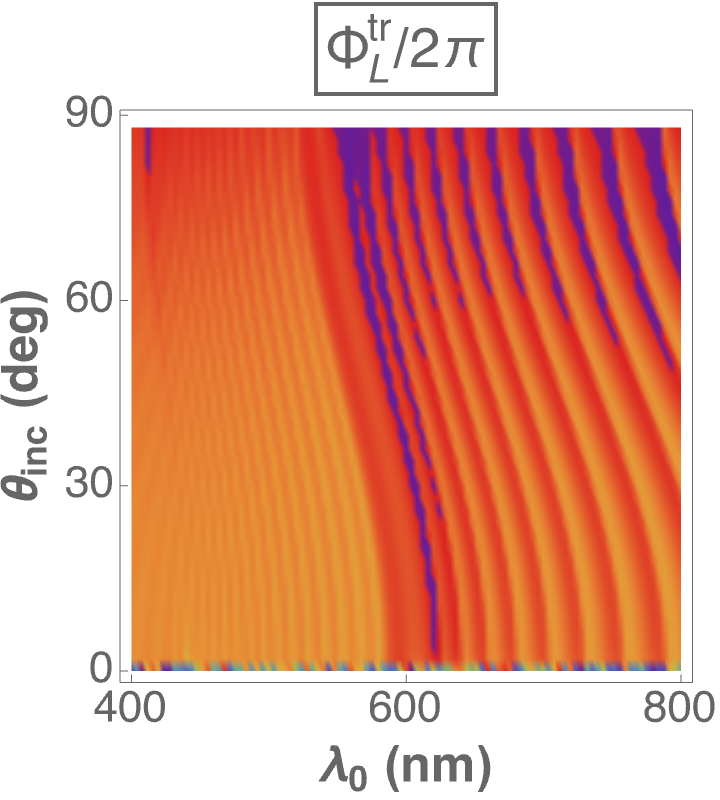
(d) $\tilde{N}=4$

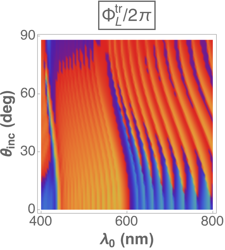
(e) $\tilde{N}=5$

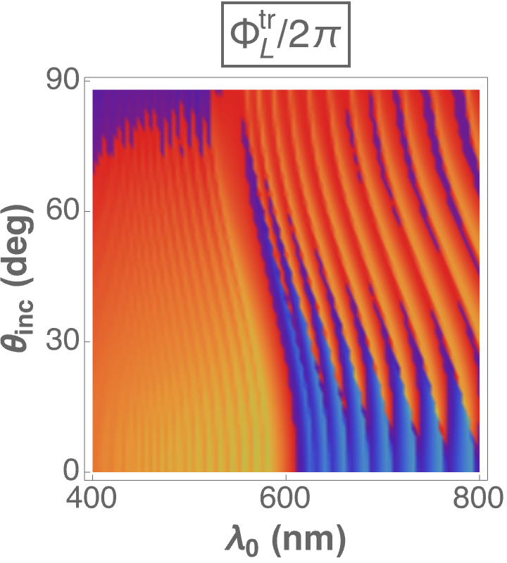
(f) $\tilde{N}=6$

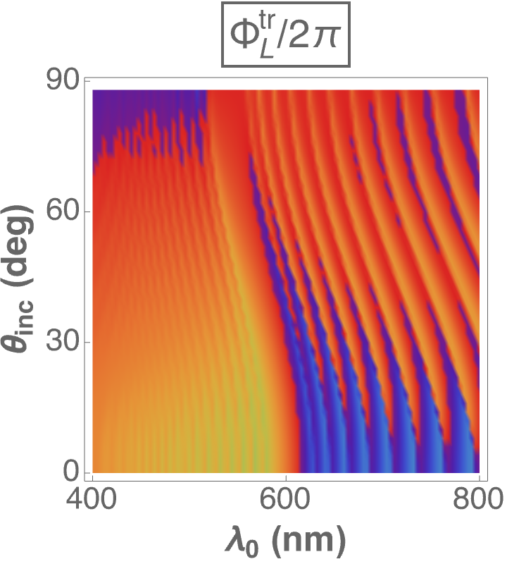
(g) $\tilde{N}=8$

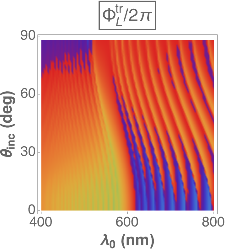
(h) $\tilde{N}=10$

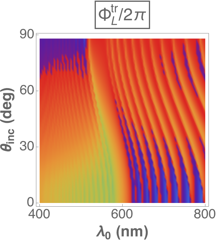
(i) $\tilde{N}=20$

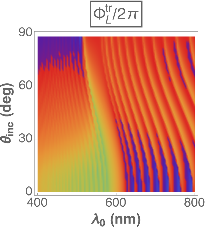
(j) $\tilde{N}=50$

Figure 20: Spectrums of $\Phi^{\rm tr}_{L}$ for $\theta_{\rm inc}\in[0^{\circ},90^{\circ})$ and $\tilde{N}\in\left\{1,2,3,4,5,6,8,10,20,50\right\}$, when $h=1$, $N=15$, $P=300$ nm, and $\psi=0^{\circ}$.

(a) $\tilde{N}=1$

References

- [1] Pancharatnam, S.: Generalized theory of interference, and its applications. Part I. Coherent pencils. Proceedings of the Indian Academy of Sciences 44, 247–262 (1956).
- [2] Shapere, A., Wilczek, F. (eds): Geometric Phases in Physics. World Scientific, Singapore (1989).
- [3] Cohen, E., Larocque, H., Bouchard, F., Nejadsattari, F., Gefen, Y., Karimi, E.: Geometric phase from Aharonov–Bohm to Pancharatnam–Berry and beyond. Nature Reviews Physics 1, 437–449 (2019).
- [4] Citro, R., Durante, O.: The geometric phase: Consequences in classical and quantum physics. In: Citro, R., Lewenstein, M., Rubio, A., Schleich, W.P., Well, J.D., Zank, G.P. (eds): Sketches of Physics: The Celebration Collection, pp. 63–84. Springer, Cham, Switzerland (2023).
- [5] Kobashi, J., Yoshida, H., Ozaki, M.: Planar optics with patterned chiral liquid crystals. Nature Photonics 11, 389–392 (2016).
- [6] Rafayelyan, M., Agez, G., Brasselet, E.: Ultrabroadband gradient-pitch Bragg–Berry mirrors. Physical Review A 96, 043862 (2017).
- [7] Balthasar Mueller, J. P., Rubin, N.A., Devlin, R.C., Groever, B., Capasso, F.: Metasurface polarization optics: Independent phase control of arbitrary orthogonal states of polarization. Physical Review Letters 118, 113901 (2017).
- [8] Jisha, C. P., Nolte, S., Alberucci, A.: Geometric phase in optics: From wavefront manipulation to waveguiding. Laser and Photonics Reviews 15, 2100003 (2021).
- [9] Hodgkinson, I. J., Wu, Q. h.: Birefringent Thin Films and Polarizing Elements. World Scientific, Singapore (1997).
- [10] Lakhtakia, A., Messier, R.: Sculptured Thin Films: Nanoengineered Morphology and Optics. SPIE, Bellingham, WA, USA (2005).
- [11] Das, A., Mandal, S., Fiallo, R.A., Horn, M.W., Lakhtakia, A., Pradhan, M.: Geometric phase and photonic spin Hall effect in thin films with architected columnar morphology. Journal of the Optical Society of America B 40, 2418–2428 (2023). Replace “” by “” in Eq. (5b).
- [12] Martin, P. M.: Handbook of Deposition Technologies for Films and Coatings, 3rd ed. Elsevier, Oxford, United Kingdom (2010).
- [13] Juodkazis, S., Mizeikis, V., Misawa, H.: Three-dimensional microfabrication of materials by femtosecond lasers for photonics applications. Journal of Applied Physics 106, 051101 (2009).
- [14] Thiel, M., Fischer, H., von Freymann, G., Wegener, M.: Three-dimensional chiral photonic superlattices. Optics Letters 35, 166–168 (2010).
- [15] Kim, H.S., Hwang, S.O., Myung, Y., Park, J.: Three-dimensional structure of helical and zigzagged nanowires using electron tomography. Nano Letters 8, 551–557 (2005).
- [16] Ding, K., Ai, J., Deng, Q., Huang, B., Zhou, C., Duan, T., Duan, Y., Han, L., Jiang, J., Che, S.: Chiral mesoporous BiOBr films with circularly polarized colour response. Angewandte Chemie International Edition 60, 19024–19029 (2021).
- [17] Kelly, J.A., Giese, M., Shopsowitz, K.E., Hamad, W.Y., MacLachlan, M.J.: The development of chiral nematic mesoporous materials. Accounts of Chemical Research 47, 1088–1096 (2014).
- [18] Yeom, J., Yeom, B., Chan, H., Smith, K.W., Dominguez-Medina, S., Bahng, J.H., Zhao, G., Chang, W.-S., Chang, S.-J., Chuvilin, A., Melnikau, D., Rogach, A.L., Zhang, P., Link, S., Král, P., Kotov, N.A.: Chiral templating of self-assembling nanostructures by circularly polarized light. Nature Materials 14, 66–72 (2015).
- [19] Hodgkinson, I.J., Lakhtakia, A., Wu, Q.h., De Silva, L., McCall, M.W.: Ambichiral, equichiral and finely chiral layered structures. Optics Communications 239, 353–358 (2004).
- [20] Reusch, E.: Untersuchung über Glimmercombinationen. Annalen der Physik und Chemie (Leipzig) 138 , 628–638 (1869).
- [21] Zaidi, Q.: Last but not the least. Perception 34, 121–123 (2005). DOI: 10.1068/p5359
- [22] Joly, G., Billard, J.: Quelques champs électromagnétiques dans les piles de Reusch II. Piles éclairées sous l’incidence normale par des ondes monochromatiques planes et uniformes. Journal de Optique (Paris) 13, 227–238 (1982).
- [23] Joly, G., Billard, J.: Quelques champs électromagnétiques dans les piles de Reusch IV. Domaines multiples de réflexion sélective. Journal de Optique (Paris) 17, 211–221 (1986).
- [24] Faryad, M., Lakhtakia, A.: The circular Bragg phenomenon. Advances in Optics and Photonics 6, 225–292 (2014).
- [25] Kinsler, P.: How to be causal: time, spacetime and spectra. European Journal of Physics 32, 1687–1700 (2011).
- [26] Lakhtakia, A., Moyer, J.T.: Post- versus pre-resonance characteristics of axially excited chiral sculptured thin films. Optik 113, 97–99 (2002).
- [27] Wang, J., Lakhtakia, A., Geddes III, J.B.: Multiple Bragg regimes exhibited by a chiral sculptured thin film half-space on axial excitation. Optik 113, 213–221 (2002).
- [28] Nityananda, R.: On the theory of light propagation in cholesteric liquid crystals. Molecular Crystals and Liquid Crystals 21, 315–331 (1973).
- [29] Garoff, S., Meyer, R.B., Barakat, R.: Kinematic and dynamic light scattering from the periodic structure of a chiral smectic liquid crystal. Journal of the Optical Society of America 68, 1217–1225 (1978).
- [30] Oldano, C., Allia, P., Trossi, L., Optical properties of anisotropic periodic helical structures. Journal de Physique (Paris) 46, 573–582 (1985).
- [31] Abdulhalim, I., Benguigui, L., Weil, R.: Selective reflection by helicoidal liquid crystals. Results of an exact calculation using the 44 characteristic matrix method. Journal de Physique (Paris) 46, 815–825 (1985).
- [32] Erten, S., Lakhtakia, A., Barber, G.D.: Experimental investigation of circular Bragg phenomenon for oblique incidence. Journal of the Optical Society of America A 32, 764–770 (2015).
- [33] McAtee, P.D., Lakhtakia, A.: Experimental and theoretical investigation of the co-occurrence of linear and circular dichroisms for oblique incidence of light on chiral sculptured thin films. Journal of the Optical Society of America A 35, 1131–1139 (2018). Replace “” by “” in Eq. (8b).
- [34] Rudakova, N.V., Timofeev, I.V., Vetrov, S.Y., Lee, W.: All-dielectric polarization-preserving anisotropic mirror. OSA Continuum 1, 682–689 (2018).
- [35] Fiallo, R.A., Lakhtakia, A., Horn, M.W.: Polarization-universal bandgaps realized with columnar thin films. Journal of Nanophotonics 16, 046004 (2022).
- [36] van Popta, A.C., Brett, M.J., Sit, J.C.: Double-handed circular Bragg phenomena in polygonal helix thin films. Journal of Applied Physics 98, 083517 (2005).
- [37] Joly, G., Billard, J.: Quelques champs électromagnétiques dans les piles de Reusch III. Biréfringence elliptique des vibrations itératives; activité optique de piles hélicoĭdales d’extension finie. Journal de Optique (Paris) 16, 203–213 (1985).
- [38] Babaei, F.: On optical rotation and selective transmission in ambichiral sculptured thin films. Journal of Modern Optics 60, 1370–1375 (2013).
- [39] Abdulhalim, I.: Effect of the number of sublayers on axial optics of anisotropic helical structures. Applied Optics 47, 3002–3008 (2008).
- [40] Babaei, F.: On circular Bragg regimes in ellipsometry spectra of ambichiral sculptured thin films. Journal of Modern Optics 60, 886–890 (2013).
- [41] Faryad, M., Lakhtakia, A.: Evolution of surface-plasmon-polariton and Dyakonov– Tamm waves with the ambichirality of a partnering dielectric material. Journal of Nanophotonics 8, 083082 (2014).
- [42] Vepachedu, V., McAtee, P.D., Lakhtakia, A.: Nonexhibition of Bragg phenomenon by chevronic sculptured thin films: experiment and theory. Journal of Nanophotonics 11, 036018 (2017).
- [43] Lakhtakia, A., Venugopal, V.C.: On Bragg reflection by helicoidal bianisotropic mediums. Archiv für Elektronik und Übertragungstechnik 53, 287–290 (1999).
- [44] Mackay, T.G., Lakhtakia, A.: The Transfer–Matrix Method in Electromagnetics and Optics. Morgan & Claypool, San Ramon, CA, USA (2020).
- [45] Jackson, J.D.: Classical Electrodynamics, 3rd edn. Wiley, New York, NY, USA (1999).
- [46] Frisch, M.: ‘The most sacred tenet’? Causal reasoning in physics. British Journal for the Philosophy of Science 60, 459–474 (2009).
- [47] Silva, H., Gross, B.: Some measurements on the validity of the principle of superposition in solid dielectrics. Physical Review 60, 684–687 (1941).
- [48] Kittel, C.: Introduction to Solid State Physics. Wiley Eastern, New Delhi, India (1974).
- [49] Mackay, T.G., Lakhtakia, A.: Modeling columnar thin films as platforms for surface–plasmonic–polaritonic optical sensing. Photonics and Nanostructures – Fundamentals and Applications 8, 140–149 (2010).
- [50] Perot, A., Fabry, C.: On the application of interference phenomena to the solution of various problems of spectroscopy and metrology. Astrophysical Journal 9, 87–115 (1899).
- [51] Lakhtakia, A.: Transmission-mode geometric-phase signatures of circular Bragg phenomenon. Journal of the Optical Society of America B 41, 500–507 (2024).
- [52] Lakhtakia, A.: Geometric phase in plane-wave transmission by a dielectric structurally chiral slab with a central phase defect. Physical Review A 109, 053517 (2024).
- [53] Lakhtakia, A., Messier, R.: Reflection at the Motohiro–Taga interface of two anisotropic materials with columnar microstructures. Optical Engineering 33, 2529–2534 (1994).
- [54] Slepyan, G.Y., Maksimenko, A.S.: Motohiro–Taga interface in sculptured thin films—absence of Bragg phenomena. Optical Engineering 37, 2843–2847 (1998).