Single-shot volumetric fluorescence imaging with neural fields

Abstract

Single-shot volumetric fluorescence (SVF) imaging offers a significant advantage over traditional imaging methods that require scanning across multiple axial planes as it can capture biological processes with high temporal resolution across a large field of view. Existing SVF imaging methods often require large, complex point spread functions (PSFs) to meet the multiplexing requirements of compressed sensing, which limits the signal-to-noise ratio, resolution and/or field of view. In this paper, we introduce the QuadraPol PSF combined with neural fields, a novel approach for SVF imaging. This method utilizes a cost-effective custom polarizer at the back focal plane and a polarization camera to detect fluorescence, effectively encoding the 3D scene within a compact PSF without depth ambiguity. Additionally, we propose a reconstruction algorithm based on the neural fields technique that addresses the inaccuracies of phase retrieval methods used to correct imaging system aberrations. This algorithm combines the accuracy of experimental PSFs with the long depth of field of computationally generated retrieved PSFs. QuadraPol PSF, combined with neural fields, significantly reduces the acquisition time of a conventional fluorescence microscope by approximately 20 times and captures a 100 mm³ cubic volume in one shot. We validate the effectiveness of both our hardware and algorithm through all-in-focus imaging of bacterial colonies on sand surfaces and visualization of plant root morphology. Our approach offers a powerful tool for advancing biological research and ecological studies.

1 Introduction

Fluorescence imaging is an indispensable tool in biological research due to its high sensitivity, its biological specificity, and its non-invasive nature, which allow for real-time observation of live organisms. To overcome the limitations of conventional 2D fluorescence microscopy and capture the full 3D structure of biological scenes, techniques such as confocal and light sheet fluorescence microscopy have been widely used. However, these methods require scanning multiple axial planes, significantly increasing the acquisition time and limiting the spatial-temporal throughput. The extensive scanning time is impractical for numerous applications where imaging large fields of view (FOVs) is required, such as when performing lab studies of the complex biological processes associated with the rhizosphere [1] - the media-root interfaces of plants.

Single-shot volumetric fluorescence (SVF) imaging techniques have been developed to address the challenges in scanning-based 3D imaging methods [2, 3, 4, 5, 6]. These methods encode volumetric data into a single 2D image, which allow for computational reconstruction of the object. One prominent technique is the light field microscope [2, 3, 4], which utilizes a standard microlens array to enable 3D capabilities. Recently, lensless architectures using coded masks or randomized microlens diffusers, have also been demonstrated [7, 8, 9, 5, 10].

While these approaches are effective, they typically suffer from limited resolution. A significant challenge with these systems is that their point spread functions (PSFs) are not shift-invariant laterally, necessitating extensive calibration to define the PSF accurately and restricting measurement to the pre-calibrated volume. Further, the shift-variant nature of the PSF complicates the image analysis – reconstructions typically require optimization algorithms that impose sparsity constraints. Another drawback of using coded masks or microlens arrays is that, not only does the large size decrease the peak signal level of the PSF by spreading photons over a larger area, photons from various axial and lateral positions overlapping on the sensor further degrade the signal-to-noise ratio (SNR). To address some of these issues while improving resolution, Miniscope3D [11] replaces the tube lens in a standard fluorescence microscope with an optimized phase mask, but it still suffers from the fundamental limitations associated with a non-compact PSF.

PSF engineering is an alternative approach that modulates the fluorescence at the back focal plane (BFP) of the objective lens in the imaging system to encode the axial position of the emitters within compact PSFs. Numerous 3D PSFs have been proposed over the past two decades [12, 13], including the astigmatic PSF [14], which varies in elongation direction and magnitude with defocus; the corkscrew [15] and double-helix [16] PSFs, which feature revolving spots around the emitter; and the tetrapod [17] and pixOL [18] PSFs, which are optimized for maximizing the Fisher information. Another group of PSFs, including the bisected [19], quadrated [20], tri-spot PSFs [21], and the multi-view reflector (MVR) microscope [22], images subapertures off the pupil center to induce lateral displacements in the focal point; the displacement direction depends on the position of the subaperture relative to the center of the BFP, and the displacement amount is proportional to the defocus.

While these engineered PSFs have proven effective primarily in single molecule localization microscopy [23, 24, 25, 26] where isolated point sources are imaged, reconstructing more complex geometries from these PSFs remains challenging. Unlike methods like Miniscope3D, compact PSFs usually cannot satisfy the multiplexing requirement of compressed sensing. Therefore, recovering the 3D object using a single image often results in ambiguities in depth measurements [27, 28]. Although using multiple images with engineered PSFs has the ability to substantially reduce these ambiguities, such as in the Fourier light field microscope [29, 30] and complex-field and fluorescence microscopy using the aperture scanning technique (CFAST) [28], these methods require either capturing multiple images sequentially at the expense of temporal resolution, or utilizing different areas of the detector to perform spatial multiplexing, thus sacrificing the FOV. A recent approach, the polarized spiral PSF [27], integrates polarizers with a double-helix phase mask and employs orthogonally polarized detection channels from a polarization camera to achieve single-shot 3D imaging without sacrificing either the temporal resolution or the FOV. However, it has not completely eliminated the ambiguity problem.

Another critical aspect in SVF imaging is the reconstruction algorithm; a robust reconstruction algorithm is essential for accurately and precisely reconstructing 3D scenes from 2D measurements captured with engineered PSFs. The Richardson-Lucy (RL) algorithm [29, 31, 32] is broadly used due to its effectiveness in recovering 3D structures. However, the reconstruction quality using this algorithm heavily depends on the accuracy of the forward model, particularly the PSF used. While experimentally calibrated PSFs can account for imperfections in the imaging system and improve the reconstruction quality, they can be inaccurate or unavailable due to system limitations or discrepancies in the forward imaging model. To address this limitation, we adopt the concept of neural fields in our work.

Neural fields have become a prominent technique for 3D scene representations and graphics rendering [33, 34]. Its concept focuses on the mapping between spatial coordinates and image intensity values using a compact multi-layer perceptron (MLP) model and optionally learnable positional embeddings. This approach has recently been applied to improve microscopic systems. For example, it has been implemented for 3D refractive index reconstruction in intensity diffraction tomography, which allows for the generation of continuous image functions across the axial dimension [35], though it required extensive optimization time on high-performance graphics processing units (GPUs). Further developments reduced the computational resources by creating an additional hash encoding layer at the input of the neural network for 2D microscopic imaging systems [36]. More adaptations of the neural fields approach include a 2D version for lensless imaging phase retrieval [37] and the modeling of space-time dynamics with 4D neural fields in imaging through scattering [38], computational adaptive optics [39], and structured illumination microscopy [40]. Advancements continued with the exploitation of redundancies in Fourier ptychographic microscopes to augment the MLP model with a compact learnable feature space, thereby speeding up the image stack reconstructions and reducing data storage burdens [41]. Most recently, the integration of neural fields with diffusion models has been proposed to aid volumetric reconstruction [42].

In this paper, we present QuadraPol PSF, an engineered PSF designed for SVF imaging that is easy to implement and overcomes the limitations of existing techniques. Additionally, we introduce a reconstruction algorithm based on neural fields that outperforms the widely used RL deconvolution. Our work is inspired by the algorithm architectures from [38, 41, 42] and redesigns them to enhance the capabilities of our imaging system, demonstrated through fluorescence imaging over a centimeter-scale lateral FOV, with a depth of 5 mm, a lateral resolution of $\sim$5 µm, and an axial resolution of $\sim$130 µm. Specifically tailored for studies of the rhizosphere, QuadraPol PSF enables all-in-focus imaging of bacterial colonies on sand surfaces and 3D visualization of plant root morphology. Our results highlight the potential of QuadraPol PSF combined with neural fields to significantly advance biological studies by providing rapid, high-resolution 3D images of complex biological structures with a large FOV.

2 Methods

2.1 Imaging system

The experimental setup of our SVF imaging system with the QuadraPol PSF is shown in Figure 1(a). We modulate a 568 nm laser (Coherent Sapphire 568 LP) transmitted through a single-mode fiber (Thorlabs P3-460B-FC-2) using a quarter-wave plate (QWP, Thorlabs WPQ10M-561) to produce circularly polarized excitation at the sample. An achromatic doublet lens (Thorlabs AC254-080-A) is used as the objective lens (OL), providing access to the back focal plane (BFP) without the need for additional 4f systems, thus simplifying the setup. The collected fluorescence is then filtered by a dichroic mirror (DM, Semrock Di01-R488/561) and a bandpass filter (BF, Semrock FF01-523/610), and modulated by a custom 4-polarization polarizer (4-Pol). The modulated fluorescence is then focused onto a polarization camera (The Imaging Source DZK 33UX250) using a tube lens (TL, Thorlabs AC254-150-A). This compact system is mounted on a $z$-stage (Newport 436, controlled by Newport CONEX-LTA-HS) and a custom-built $xy$ gantry system (Ballscrew SFU1605 with NEMA23 Stepper Motor) capable of scanning a 200$\times$200 mm² area.

The 4-Pol custom polarizer (Figure 1(b)) is constructed by cutting four pieces from a thermoplastic polymer film linear polarizer (Thorlabs LPVISE2X2) with a laser cutter (Universal Laser Systems PLS6.75), and positioning them between two circular coverslips (VWR 48380-046). Two 3D-printed (Anycubic Photon Mono X 6Ks) holders apply clamping forces to secure the polarizers and coverslips, preventing displacement. One holder features a 9-mm diameter aperture to ensure the shift invariance of the imaging system’s PSF, corresponding to a numerical aperture (NA) of 0.056. Additionally, 0.6-mm lines are printed along the center of the holder to block unmodulated fluorescence from passing through gaps between the polarizers.

The polarization camera integrates a polarizer microarray atop the CMOS sensor. Typically, the raw pixel data (Figure 1(c-i)) is processed to visualize the angle of linear polarization (AoLP), which indicates the polarization direction, and the degree of linear polarization (DoLP), which quantifies the proportion of polarized fluorescence (Figure 1(c-ii)) [43, 44]. Alternatively, the data can be decomposed into images corresponding to the four polarization channels, as shown in Figure 1(c-iii).

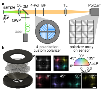
Figure 1: (a) Schematic of single-shot volumetric fluorescence imaging using the QuadraPol PSF. OL, objective lens; TL, tube lens; QWP, quarter waveplate; DM, dichroic mirror; BF, bandpass filter. A 4-polarization custom polarizer (4-Pol) is positioned at the back focal plane (BFP) of the imaging system to modulate the emission light, with a polarization camera (PolCam) capturing the modulated fluorescence. The transmission axes of the polarizer and PolCam are 0°, 45°, 90°, and 135°. (b) Assembling the custom polarizer by aligning two coverslips and four laser-cut polymer polarizers between 3D-printed holders. (c) A representative image captured by the polarization camera, visualized using (i) raw pixel readouts, (ii) a polarization image color-coded in the HSV scheme (AoLP as hue, DoLP as saturation, and intensity as value), and (iii) four separate images for each polarization channel. Scale bar: 50 µm.

2.2 Point spread function design and experimental calibration

The design of the QuadraPol PSF is inspired by the quadrated PSF [20], the MVR microscope [22], and CFAST [28]. These techniques divide the pupil into four sections. Specifically, the quadrated phase mask applies different phase ramps to each segment, generating a four-spot PSF in a single imaging channel. In contrast, the MVR and CFAST systems utilize reflective mirrors and light-blocking apertures, respectively, to create distinct image channels for each pupil segment. A key characteristic of these techniques is the encoding of the axial position of the emitter through the different lateral displacements of the focused spots, each associated with one of the four equal segments of the pupil. However, these approaches come with limitations. The single-image capture with the quadrated PSF can lead to ambiguities in 3D reconstruction, while the MVR and CFAST setups sacrifice either FOV or temporal resolution. The QuadraPol PSF distinguishes itself by modulating each pupil section using a polarizer with a unique transmission axis, allowing the polarization camera to simultaneously capture four imaging channels without losing FOV or temporal resolution.

Given the imaging system’s low NA, the theoretical PSF (Figure 2(a)) for the axial position $z$ in each polarization channel ($\mathrm{pol}\in\{0^{\circ},45^{\circ},90^{\circ},135^{\circ}\}$) can be described by (see Supplementary Section 1 for more details) [45, 46]

$$\mathrm{PSF}_{z,\mathrm{pol}}=$$

$$\sum_{i\in[p,s]}\mathcal{F}\left\{A_{\mathrm{pol},i}(u,v)\exp\left\{j\left[kz\sqrt{1-u^{2}-v^{2}}+P(u,v)\right]\right\}\right\}^{2},$$ (1)

where $k=2\pi/\lambda$ represents the wave number, and $(u,v)$ are the coordinates at the BFP. The pupil phase is consistent across all polarization channels; a uniform phase, $P(u,v)=0$, is used for calculating the unaberrated theoretical PSF. The amplitude modulation patterns for $p$- and $s$-polarizations are shown in Figure 2(a). These patterns assign values of 1, 0.5, and 0 for amplitude mask with $p$-polarization, and 0, $\pm$0.5, and 0 for $s$-polarization, corresponding to the angles between the transmission axis of the polarizers and detection channel at 0°, 45°, and 90°, respectively.

Compared to other compact PSFs, such as the double-helix [16] and spiral polarized PSFs [27], the QuadraPol PSF distinguishes itself by utilizing all available polarization channels from a polarization camera, effectively capturing three independent images. These images enable the QuadraPol PSF to completely eliminate ambiguities in depth estimation (Supplementary Figure S1 and Section 2), avoiding the need for larger, more complex PSF designs and also relaxing the sparsity constraint required for image reconstruction (Supplementary Figure S2 and Section 3). Consequently, the QuadraPol PSF also provides a better SNR compared to existing single-shot volumetric imaging techniques, despite the photon loss due to the linear polarizers (Supplementary Figure S3 and Section 3). Note that due to cross-talk between polarization channels separated by 45°, the PSF in each channel exhibits a primary spot and two weaker side spots, rather than a singular focal point (Supplementary Figure S4).

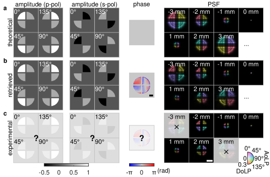
Figure 2: Amplitude and phase of the pupil and PSFs for at different heights. (a) Theoretical PSFs without aberration, (b) simulated PSFs using the retrieved phase, and (c) experimental PSFs. Scale bar: 2 mm for the pupil images, and 0.2 mm for the PSF images.

Given the presence of aberrations in our imaging system, primarily introduced by the custom-made polarizer, we use the vectorial implementation of phase retrieval [47] to compensate for these imperfections. This approach enables us to refine a series of retrieved PSFs (Figure 2(b)) that more closely match those obtained experimentally (Figure 2(c)) compared with theoretically obtained ones (Figure 2(a)). These experimental PSFs are generated by averaging images from 77 fluorescent beads (Thermo Fisher F8858), which were axially scanned over a 4 mm range with a 0.1 mm step size. The retrieved phase of the pupil is shown in Figure 2(b), while we assume that the pupil amplitude remains the same as those in Figure 2(a).

2.3 Reconstruction algorithm

Previous studies have shown the effectiveness of the modified RL deconvolution algorithm in reconstructing 3D volumetric scenes using multiple input images [29, 28]. In our work, we apply this algorithm with the experimental PSF to reconstruct samples with a $z$ range of less than 4 mm. The RL deconvolution algorithm iteratively updates the estimated object $o$ as

$$o^{(k+1)}=o^{(k)}\frac{\sum_{\mathrm{pol}}\left(I_{\mathrm{pol}}\otimes\mathrm{PSF}_{z,\mathrm{pol}}^{*}\right)}{\sum_{\mathrm{pol}}\left\{\left[\sum_{z}\left(o_{z}^{(k)}\otimes\mathrm{PSF}_{z,\mathrm{pol}}\right)\right]\otimes\mathrm{PSF}_{z,\mathrm{pol}}^{*}\right\}},$$ (2)

where $\mathrm{PSF}^{*}$ represents the original PSF with a 180° rotation in the $xy$ plane, $I_{\mathrm{pol}}$ represents the intensity from one of the polarization channels, and $\otimes$ denotes the convolution operator.

The deconvolution using experimental PSFs, acquired from the calibration experiment at discrete $z$ planes, can produce accurate reconstruction results within a certain depth range. However, rhizosphere-asscociated samples, such as plant roots, can extend to a large depth range across different FOVs. To extend the depth range for reconstruction, the naive solution would be to obtain the PSFs at larger depths. Unfortunately, with the extended depth range, the PSF will expand to a larger size, as demonstrated in Figure 2, resulting in low SNR and making it challenging to capture. An alternative method is to implement the retrieved PSFs. Because they are generated from aberrated phase terms and ideal amplitude masks, they suit the needs at arbitrary $z$ planes with continuous sampling and can extend to a farther depth range. Nevertheless, the retrieved PSF cannot reconstruct high-quality image volumes as the experimental PSF via deconvolution. The discrepancy lies in the non-ideal pupil amplitude and inaccurate pupil phase retrieval.

To address this dilemma, we customize and design the neural fields to enhance the performance of our system. Given the deconvolved image volumes from experimental and retrieved PSFs, we can start with the image volume merged from these two deconvolution results (Figure 3(a)). A two-step optimization process is then utilized. The first step is to initialize our neural field with the merged image volume. The neural field with compact learnable feature space design is a 3D feature tensor ($M$) dot product a feature tensor ($u$) [41] and it is composed of two nonlinear layers with ReLU activation functions and one linear layer. Each layer of the MLP in our neural field has $Q$ neurons with an additional offset neuron. The number of neurons is designed to match the number of feature channels in the feature space. The feature space is created from the Hadamard product of a feature tensor $M$ with a size of $N/2\times N/2\times Q$ and a feature tensor $u$ with a size of $Z\times Q$, where $N$ is the number of pixels along $x$ or $y$ axis of the raw image, $Q$ is the number of feature channels, and $Z$ denotes the number of pre-defined $z$-coordinates. The detailed parameters and hyperparameters of the neural fields can be found in Supplementary Section 4. The MLP model generates an image volume from random initialization of the feature space and is supervised by the merged image volume. This process can be modeled as finding a mapping function ($\phi$) between feature tensor space and the image volume:

$$\phi(\mathbf{x}):\mathbb{R}^{2}\cdot\mathbb{R}\mapsto\mathbb{R}^{3},\;\;\mathbb{C}(f(\mathbf{x}),\phi(\mathbf{x}))$$ (3)

where $\mathbf{x}=(x,y,z)$ represents the 3D coordinate system, $\mathbb{C}$ is a set of constraints bounded by the merged image volume $f(\mathbf{x})$.

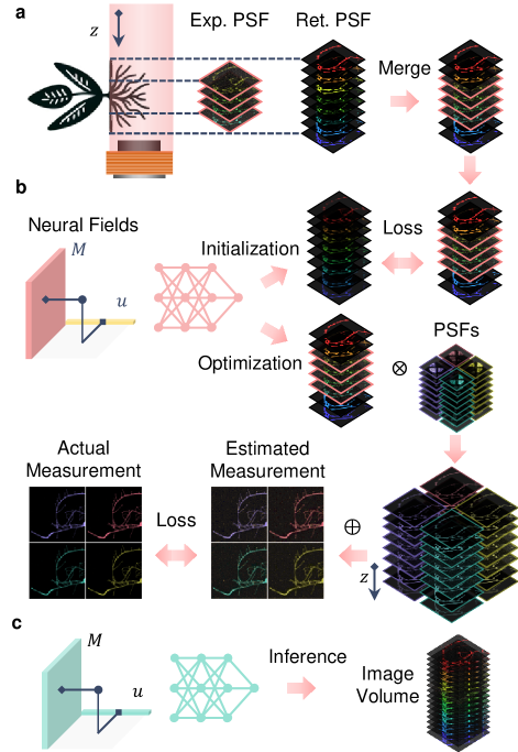
Figure 3: Framework of using neural fields to extend the quality and depth range of the imaging system. (a) The initial image volume is obtained from the deconvolution using experimental PSFs (Exp. PSFs) for central frames and retrieved PSFs (Ret. PSFs) for peripheral frames. (b) The merged image volume from (a) guides the initialization of the model with a compact lernable feature space and multilayer perceptron (MLP). After model initialization, the model is further optimized for the image volume. The estimated image volume goes through the forward model of the imaging system to generate the estimated measurements. These measurements are compared with the acquired measurements, and then to update the model weights and parameters. (c) Once the model is optimized, the parameters and weights are fixed. It can render an image stack with continuous sampling. The operator $\otimes$ denotes a convolution operation, and $\oplus$ indicates a summation operation along $z$-axis.

Once the neural field is initialized, it can render an image volume as an initial guess. This initial guess ($g$) is then fed to the forward model of the imaging system to generate estimated measurements:

$$I_{\mathrm{pol}}(x,y)=\sum_{z}|g_{z}(\mathbf{x})\otimes\mathrm{PSF}_{z,\mathrm{pol}}|^{2}$$ (4)

where $I_{\mathrm{pol}}(x,y)$ is the estimated measurements from the neural field rendered image volume, $g_{z}$ denotes the rendered image volume at one $z$-plane, and $\otimes$ is the convolution operator. The PSFs are reused from the experimental PSF and retrieved PSF for an extended depth range. The estimated measurements are then compared with the experimental intensity measurements (Figure 3(b)) to calculate a loss function value. The loss term is back-propagated to update the parameters and weights in the neural field until convergence.

After the two-step optimization is done, the parameters and weights in the neural field are fixed. We can continuously sample the feature tensor ($u$) to render a denser image volume along the axial ($z$) axis, as shown in Figure 3(c).

2.4 Sample preparation

Starting from a single colony, E. coli-mScarlet-I was grown in LB medium overnight at 37°C. On the next day, the overnight culture was washed once in minimal medium and diluted to an optical density of 1. To prepare for imaging, 1 mL of cell culture was added to 10 g of autoclaved fine sand (Fischer Science Education Sand, Cat. No. S04286-8) in a small petri dish and briefly mixed by vortexing before imaging.

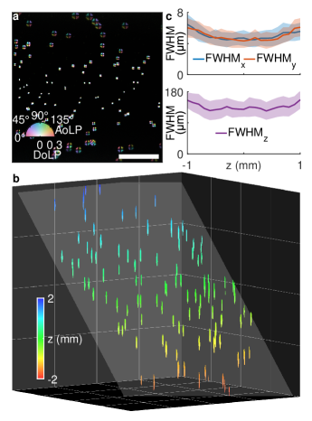
Figure 4: Imaging fluorescent beads on a 45°-tilt coverslip using the QuadraPol PSF. (a) Raw image of the fluorescent beads. Scale bar: 1 mm. (b) Three-dimensional rendering of the reconstructed beads using MATLAB function “isosurface”. Grid size: 1 mm. (c) Full width at half maximum (FWHM) values for the reconstructed beads. Lines represent the average; shaded areas represent the standard deviation.

Soft white wheat seeds were obtained from Handy Pantry (Lot 190698). Seeds were sterilized by incubating in 70% ethanol for 2 min, washing 3 times with autoclaved water, incubating with a bleach (50% v/v) and Triton X (0.1% v/v) solution for 3 min, and finally washing 5 times with autoclaved water. Seeds were then plated on 0.6% phytagel (Sigma Aldrich, Cat. No. P8169) containing 0.5x MS medium (Sigma Aldrich Cat. No. M5519) and transferred to a growth chamber with a day/night cycle of 16 hr/8 hr at 25°C for 7 days. On day 7, seedlings were collected and incubated in 100 µM merocyanine 540 (MC540) in phosphate buffered saline (PBS) for 15 min, then rinsed in DI water before imaging.

3 Results

3.1 System calibration and validation on fluorescent beads

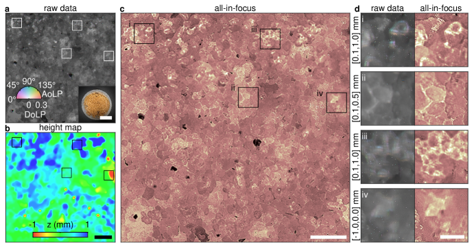
Figure 5: All-in-focus imaging of E. coli tagged with mScarlet-I on sand surfaces. (a) Raw polarized fluorescence image. The inset shows a photograph of the sample captured using a smartphone camera. (b) Height map recovered using the all-in-focus algorithm. Color bar: height in mm. (c) The all-in-focus fluorescence image. (d) The zoomed regions of interest in (a-c). Annotations represent the $z$ range for each region. Scale bar: 20 mm in the inset of (a), 2 mm in (b,c), and 0.5 mm in (d).

We first validate the 3D imaging capabilities of the QuadraPol PSF with fluorescent beads placed on a tilted coverslip (Figure 4(a)). The 3D reconstruction is shown in Figure 4(b), where the deconvolution algorithm accurately resolves the fluorescent beads on the coverslip without noticeable inaccuracies. Additionally, we quantify the full width at half maximum (FWHM) values for the reconstructed images of 72 fluorescent beads from a $z$ scan (Figure 4(c)). The FWHM values are $4.7\pm 1.0$ µm and $4.3\pm 0.9$ µm in the $x$ and $y$ directions, respectively, for in-focus beads. The average FWHM remains within 5.0 µm for a $|z|\leq 0.6$ mm. When beads are defocused by 1 mm, the FWHM increases to an average of 6.0 µm. In the $z$ direction, the average FWHM is consistently below 130.4 µm across a depth of field (DOF) of 1.2 mm, and increases to an average of 155.7 µm when defocused by 1 mm. This extended DOF is notably longer than the 0.26 mm DOF achievable with a standard PSF. The space-bandwidth product (SBP) of our system is 8.67 million voxels over the 2 mm depth range. Note that the SBP for the biological experiments in later sections is greater than the value reported here. We are not confined to the 2 mm depth range, as we can still reconstruct the object with slightly reduced resolution at greater defocus distances.

3.2 All-in-focus imaging of bacterial colony on sand surfaces

Bacterial activities play a crucial role in the biochemical processes within the rhizosphere [48]. Given the highly complex and scattering nature of soil environments, many lab-based environmental and biological experiments use sand as a proxy [49, 50, 51]. Sand offers better physical and chemical simplicity and uniformity, providing a well-controlled setting for scientific analyses. Visualizing bacterial colonies in sand represents a significant advancement toward in situ studies of bacterial behavior. However, a key challenge arises from the typical size of sand particles, which creates a non-flat surface that can cause many areas within the FOV to be out of focus when captured in a single snapshot by a standard microscope without a $z$ scan.

To address this challenge, we use 3D imaging with the QuadraPol PSF to visualize E. coli tagged with mScarlet-I on the sand surface (Figure 5(a)). Multiple FOVs are stitched together using the Microscopy Image Stitching Tool plugin in imageJ [52]. To determine the correct focusing height map (Figure 5(b)) and generate an all-in-focus image (Figure 5(c)) [53, 54], we use a $100\times 100$ pixel window (side length of 0.35 mm) sliding across the entire FOV. The sharpest focus $z$ position for each window is selected based on image contrast, defined as the difference between the 99th and 1st percentile values in each reconstructed $z$-slice (Supplementary Figure S5). The zoomed regions (Figure 5(d)) show that we successfully resolved sharp reconstructions of the bacterial colonies on the sand particles within a $z$ range of 2 mm from the blurred raw images.

3.3 Three-dimensional imaging of plant roots with neural fields

Plant roots play a critical role in the rhizosphere, serving as the primary interface between the plant and the soil, and significantly influencing the activities of soil microbes. However, visualizing roots poses significant challenges due to their typically large depth variation, which complicates the acquisition of focused images across the entire volume of interest. Here, we conduct 3D imaging of wheat roots stained with MC540 within a 5 mm-thick glass container (Figure 6(a), Starna Cells 93-G-5). The raw image (Figure 6(b)) shows how depth is encoded in the polarization of detected fluorescence. Two zoomed regions show different polarization characteristics: one shows the top of the root polarized at 0 degrees and the bottom at 90 degrees while the other exhibits the opposite pattern, indicating different defocus directions for these root segments.

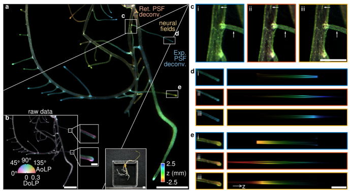
Figure 6: Volumetric imaging of wheat roots using the QuadraPol PSF. (a) Reconstruction using (blue) deconvolution with experimental PSF, (orange) deconvolution with retrieved PSF, and (yellow) neural fields. Inset shows a photograph captured using a smartphone camera. (b) The raw polarized fluorescence image. (c) The $xy$ view, and (d,e) the $xy$ and $xz$ views of zoomed regions in (a), reconstructed using (i) deconvolution with experimental PSF, (ii) deconvolution with retrieved PSF, and (iii) neural fields. Scale bar: 5 mm in (a,b), 0.5 mm in the zoomed region of (b), and 1 mm in (c-e). Color bar: depth in mm.

We perform the reconstruction using the RL deconvolution with both the experimental and retrieved PSFs, as well as our proposed method based on neural fields in Section 2.3. The image volumes with color-coded depth are presented in Figure 6. Observations from full FOV images (Figure 6(a) and Supplementary Figure S6) highlighted that for thicker segments of the roots, the deconvolution results with the experimental PSF appear closer to $z=0$ (indicated by green color in Figure 6(a)) compared to the method using neural fields. This difference is because the axial span of the root exceeds the 4 mm depth range captured for the experimental PSF (Figure 2(c)), leading to truncation at $z=\pm 2$ mm in the reconstructed object. In contrast, deconvolution with the retrieved PSF shows a broader spread in $z$, indicated by more pronounced blue ($+z$) and red ($-z$) colors in the reconstruction as well as the $z$ stack (Supplementary Figure S7), due to minor mismatches between the experimental and retrieved PSFs that reduce $z$-axis accuracy and precision. The neural field method addresses these issues by maintaining the accuracy and precision of the deconvolution with the experimental PSF while avoiding its truncation problems.

We further examine the zoomed region of a thicker part of the root (Figure 6(c)), where the neural field reconstruction (Figure 6(c-iii)) shows significantly sharper cell walls compared to the deconvolution results with either the experimental (Figure 6(c-i)) or the retrieved PSF (Figure 6(c-ii)). This improvement is attributed to our neural field method jointly taking the contribution from fluorescence signals at extended depth regions and accurate PSFs of the experimental calibrations. The enhancements in both the lateral and axial directions are also observed in out-of-focus thinner regions of the root (Figures 6(d,e)), where $xy$ views using the neural field method show sharper images and the $yz$ views exhibit a narrower spread compared to the deconvolution results using the retrieved PSF; the width mirrors the precision of the experimental PSF while overcoming its limitations of depth truncation. Improved reconstruction quality with neural fields is also demonstrated in additional zoomed regions (Supplementary Figures S8 and S9), showing mitigation of artifacts from deconvolution with the experimental PSF, and visualization of fine structures like root hairs, which cannot be resolved using deconvolution with the retrieved PSF.

4 Discussion and conclusion

Our proposed method combines the QuadraPol PSF with neural fields to achieve SVF imaging. A major innovation in hardware is the usage of the four-polarization custom polarizer, which simultaneously encodes depth information across four images (three of which are independent) captured by a polarization camera. This setup maximizes the capabilities of the polarization camera, completely eliminating the estimation ambiguity while maintaining a compact footprint, which allows the QuadraPol PSF to achieve a better SNR compared to the state-of-the-art SVF technique. With a single FOV of 3.8 mm $\times$ 4.5 mm, we experimentally demonstrate the ability to capture a $\sim$100 mm³ cubic volume with lateral and axial resolutions of up to 4 µm and 130 µm, respectively. The extended DOF offered by this system reduces acquisition time by approximately 20 times compared to traditional $z$-scan methods for capturing the same volume. The effectiveness of the QuadraPol PSF is shown in our all-in-focus imaging of bacterial colonies on sand surfaces, where it captures sharp images of most of the colonies in a single snapshot.

For the reconstruction algorithm, neural fields address limitations of classical reconstruction algorithms. By combining both experimental and retrieved PSFs, our method resolves two major issues: first, the truncation artifacts in deconvolution using experimental PSF, caused by a limited $z$ range during calibration data capture; and second, the reduced accuracy of deconvolution using retrieved PSFs due to imperfect imaging system modeling. As demonstrated in our plant root imaging experiments, nerual fields produce sharper images compared to deconvolution. The neural field approach also offers additional advantages such as creating a continuous representation of the object and significantly decreasing data storage requirements by an order of magnitude. For instance, storing plant root data as discrete images with 81 axial slices requires approximately 62 GB, whereas neural fields of the same data requires only 6.12 GB with the same data precision.

SVF imaging using the QuadraPol PSF and neural fields provides a powerful tool for large-FOV imaging at high spatial-temporal resolutions. The design principle can be easily adapted to meet specific application requirements. For instance, our current setup prioritizes high temporal resolution by using a polarization camera with a large effective pixel size, thus sacrificing spatial resolution. However, systems requiring higher spatial sampling rate from the detector could use a standard camera combined with polarization optical elements and temporal multiplexing to address this limitation. In summary, our experimental results highlight its potential, particularly for applications such as studying microbial interactions within the rhizosphere. It also paves the way for new developments in hardware and algorithm designs for SVF imaging techniques.

Funding The work reported in this paper is supported by the Resnick Sustainability Institute and the Heritage Medical Research Institute (HMRI-15-09-01) at Caltech.

Acknowledgments We thank Tara Chari for constructing the E. coli strain harboring mScarlet-I. We also thank Daniel Wagenaar from the Caltech Neurotechnology lab for the assistance in fabricating the custom polarizer and Panlang Lyu for the helpful discussions.

Disclosures The authors declare no conflicts of interest.

Supplemental document See Supplemental Document for supporting content.

References

- [1] P. Prashar, N. Kapoor, and S. Sachdeva, \JournalTitleReviews in Environmental Science and Bio/Technology 13, 63 (2014).
- [2] M. Levoy, R. Ng, A. Adams, et al., \JournalTitleACM Transactions on Graphics 25, 924 (2006).
- [3] M. Broxton, L. Grosenick, S. Yang, et al., \JournalTitleOptics Express 21, 25418 (2013).
- [4] O. Skocek, T. Nöbauer, L. Weilguny, et al., \JournalTitleNature Methods 15, 429 (2018).
- [5] Y. Xue, I. G. Davison, D. A. Boas, and L. Tian, \JournalTitleScience Advances 6, eabb7508 (2020).
- [6] V. Boominathan, J. T. Robinson, L. Waller, and A. Veeraraghavan, \JournalTitleOptica 9, 1 (2022).
- [7] J. K. Adams, V. Boominathan, B. W. Avants, et al., \JournalTitleScience Advances 3, e1701548 (2017).
- [8] N. Antipa, G. Kuo, R. Heckel, et al., \JournalTitleOptica 5, 1 (2018).
- [9] G. Kuo, F. Linda Liu, I. Grossrubatscher, et al., \JournalTitleOptics Express 28, 8384 (2020).
- [10] F. Tian, J. Hu, and W. Yang, \JournalTitleLaser & Photonics Reviews 15, 2100072 (2021).
- [11] K. Yanny, N. Antipa, W. Liberti, et al., \JournalTitleLight: Science & Applications 9, 171 (2020).
- [12] L. Von Diezmann, Y. Shechtman, and W. E. Moerner, \JournalTitleChemical Reviews 117, 7244 (2017).
- [13] E. Nehme, D. Freedman, R. Gordon, et al., \JournalTitleNature Methods 17, 734 (2020).
- [14] B. Huang, W. Wang, M. Bates, and X. Zhuang, \JournalTitleScience 319, 810 (2008).
- [15] M. D. Lew, S. F. Lee, M. Badieirostami, and W. E. Moerner, \JournalTitleOptics Letters 36, 202 (2011).
- [16] S. R. P. Pavani, M. A. Thompson, J. S. Biteen, et al., \JournalTitleProceedings of the National Academy of Sciences 106, 2995 (2009).
- [17] Y. Shechtman, L. E. Weiss, A. S. Backer, et al., \JournalTitleNano Letters 15, 4194 (2015).
- [18] T. Wu, J. Lu, and M. D. Lew, \JournalTitleOptica 9, 505 (2022).
- [19] A. S. Backer, M. P. Backlund, A. R. von Diezmann, et al., \JournalTitleApplied Physics Letters 104, 193701 (2014).
- [20] A. S. Backer, M. P. Backlund, M. D. Lew, and W. E. Moerner, \JournalTitleOptics Letters 38, 1521 (2013).
- [21] O. Zhang, J. Lu, T. Ding, and M. D. Lew, \JournalTitleApplied Physics Letters 113, 031103 (2018).
- [22] O. Zhang, Z. Guo, Y. He, et al., \JournalTitleNature Photonics 17, 179 (2023).
- [23] S. T. Hess, T. P. Girirajan, and M. D. Mason, \JournalTitleBiophysical Journal 91, 4258 (2006).
- [24] M. J. Rust, M. Bates, and X. Zhuang, \JournalTitleNature Methods 3, 793 (2006).
- [25] E. Betzig, G. H. Patterson, R. Sougrat, et al., \JournalTitleScience 313, 1642 (2006).
- [26] M. Lelek, M. T. Gyparaki, G. Beliu, et al., \JournalTitleNature Reviews Methods Primers 1, 39 (2021).
- [27] B. Ghanekar, V. Saragadam, D. Mehra, et al., \JournalTitleIEEE Transactions on Pattern Analysis and Machine Intelligence pp. 1–12 (2024).
- [28] O. Zhang, R. E. Alcalde, H. Zhou, et al., “Investigating 3D microbial community dynamics in the rhizosphere using complex-field and fluorescence microscopy,” (2024).
- [29] C. Guo, W. Liu, X. Hua, et al., \JournalTitleOptics Express 27, 25573 (2019).
- [30] K. Han, X. Hua, V. Vasani, et al., \JournalTitleBiomedical Optics Express 13, 5574 (2022).
- [31] A. C. Kak and M. Slaney, Principles of Computerized Tomographic Imaging (Society for Industrial and Applied Mathematics, 2001).
- [32] F. Dell’Acqua, G. Rizzo, P. Scifo, et al., \JournalTitleIEEE Transactions on Biomedical Engineering 54, 462 (2007).
- [33] J. J. Park, P. R. Florence, J. Straub, et al., \JournalTitle2019 IEEE/CVF Conference on Computer Vision and Pattern Recognition (CVPR) pp. 165–174 (2019).
- [34] B. Mildenhall, P. P. Srinivasan, M. Tancik, et al., “Nerf: Representing scenes as neural radiance fields for view synthesis,” in ECCV, (2020).
- [35] R. Liu, Y. Sun, J. Zhu, et al., \JournalTitleNat. Mach. Intell. 4, 781 (2022).
- [36] S. Xie, H. Zhu, Z. Liu, et al., “Diner: Disorder-invariant implicit neural representation,” in Proceedings of the IEEE/CVF Conference on Computer Vision and Pattern Recognition, (2023).
- [37] H. Zhu, Z. Liu, Y. Zhou, et al., \JournalTitleOpt. Express 30, 18168 (2022).
- [38] B. Y. Feng, H. Guo, M. Xie, et al., \JournalTitleScience Advances 9 (2023).
- [39] I. Kang, Q. Zhang, S. X. Yu, and N. Ji, “Coordinate-based neural representations for computational adaptive optics in widefield microscopy,” (2024).
- [40] R. Cao, N. Divekar, J. Nuñez, et al., \JournalTitlebioRxiv (2024).
- [41] H. Zhou, B. Y. Feng, H. Guo, et al., \JournalTitleOptica 10, 1679 (2023).
- [42] M. Hui, Z. Wei, H. Zhu, et al., “Microdiffusion: Implicit representation-guided diffusion for 3d reconstruction from limited 2d microscopy projections,” (2024).
- [43] M. Born and E. Wolf, Principles of optics: electromagnetic theory of propagation, interference and diffraction of light (Elsevier, 2013).
- [44] E. Bruggeman, O. Zhang, L.-M. Needham, et al., “POLCAM: Instant molecular orientation microscopy for the life sciences,” (2023).
- [45] L. Novotny and B. Hecht, Principles of Nano-Optics (Cambridge University Press, Cambridge, England, 2012).
- [46] A. S. Backer and W. E. Moerner, \JournalTitleThe Journal of Physical Chemistry B 118, 8313 (2014).
- [47] B. Ferdman, E. Nehme, L. E. Weiss, et al., \JournalTitleOptics Express 28, 10179 (2020).
- [48] N. A. FUJISHIGE, N. N. KAPADIA, and A. M. HIRSCH, \JournalTitleBotanical Journal of the Linnean Society 150, 79 (2006).
- [49] A. V. Vollsnes, C. M. Futsaether, and A. G. Bengough, \JournalTitleEuropean Journal of Soil Science 61, 926 (2010).
- [50] D. Probandt, T. Eickhorst, A. Ellrott, et al., \JournalTitleThe ISME Journal 12, 623 (2018).
- [51] F. Anselmucci, E. Andò, G. Viggiani, et al., \JournalTitleScientific Reports 11, 22262 (2021).
- [52] J. Chalfoun, M. Majurski, T. Blattner, et al., \JournalTitleScientific Reports 7, 4988 (2017).
- [53] Z. Bian, C. Guo, S. Jiang, et al., \JournalTitleJournal of Biophotonics 13, e202000227 (2020).
- [54] M. Liang, C. Bernadt, S. B. J. Wong, et al., \JournalTitleJournal of Pathology Informatics 13, 100119 (2022).