Prediction in Measurement Error Models

Abstract

We study the well known difficult problem of prediction in measurement error models. By targeting directly at the prediction interval instead of the point prediction, we construct a prediction interval by providing estimators of both the center and the length of the interval which achieves a pre-determined prediction level. The constructing procedure requires a working model for the distribution of the variable prone to error. If the working model is correct, the prediction interval estimator obtains the smallest variability in terms of assessing the true center and length. If the working model is incorrect, the prediction interval estimation is still consistent. We further study how the length of the prediction interval depends on the choice of the true prediction interval center and provide guidance on obtaining minimal prediction interval length. Numerical experiments are conducted to illustrate the performance and we apply our method to predict concentration of $A\beta 1-42$ in cerebrospinal fluid in an Alzheimer’s disease data.

and

1 Introduction

Prediction in measurement error models is a notoriously difficult problem. In fact, prediction has been largely avoided in the measurement error literature except for a few works (Ganse et al., 1983; Buonaccorsi, 1995; Carroll et al., 2009; Datta et al., 2018) in special cases, because the difficulties involved are fundamental and almost impossible to overcome. Instead, a different notion of prediction is sometimes used, where although the observed data contain measurement errors, the “prediction” is conducted for observed covariates that are error free, thus changing the true notion of prediction (Zhang et al., 2019, 2021).

The difficulty involved in prediction for measurement error models is rooted in the problem setting itself, in that the task of prediction involves issues beyond the model estimation itself. Indeed, even if the measurement error model is completely known without any unknown parameters, prediction is still unachievable. To see this, assume we have response variable $Y$ and covariate $X$ that is subject to measurement error. Instead of $X$, we observe $W$, which is linked to $X$ via $W=X+U$. A typical and simplest measurement error model specifies the dependence of $Y$ on $X$ up to some unknown parameters, say ${\bm{\beta}}$, and the relation between $W$ and $X$. Given independent and identically distributed (iid) observations $(W_{i},Y_{i}),i=1,\dots,n$, various methods have been developed to estimate the unknown parameter ${\bm{\beta}}$. The goal of prediction in the measurement error model context is to further estimate $Y_{n+1}$ based on a new $W_{n+1}$, while making use of the link between $Y$ and $X$ and the link between $W$ and $X$. This implies that we are obliged to study the dependence of $Y$ on $W$, which is not readily available even though we can estimate ${\bm{\beta}}$. To see this, $f_{Y,W}(y,w)=\int f_{Y\mid X}(y,x,{\bm{\beta}})f_{W\mid X}(w,x)f_{X}(x)d\mu(x)$, and without the knowledge of the probability density function (pdf) $f_{X}(x)$, even after we obtain the estimation for ${\bm{\beta}}$, we still cannot obtain $f_{Y\mid W}(y,w)$. Here, we use $f_{Y\mid W}(y,w)$ to denote the conditional pdf of $Y$ given $W$, and similarly for other notations. Of course, as often raised by people who dismiss measurement error literatures, one can always directly study the relation between the response $Y$ and the errored covariates $W$. Although it is certainly a natural and valid idea, this approach gives up the existing knowledge on the relation between the response and the original covariate $X$, i.e. the model $f_{Y\mid X}(y,x,{\bm{\beta}})$, hence giving up any inherent relation between $Y$ and $W$ as well. Indeed, the information contained in a completely unspecified function $f_{Y\mid W}(y,w)$ and a partially specified function $\int f_{Y\mid X}(y,x,{\bm{\beta}})f_{W\mid X}(w,x)f_{X}(x)d\mu(x)$ is not the same, even though on the surface both contain a single nonparametric component. In fact, in our numerical experiments, we found that taking into account the existing relation $f_{Y\mid X}(y,x,{\bm{\beta}})$ improves the prediction quite substantially in comparison to a direct approach to predict $Y$ based on $W$.

In this work, instead of providing a single prediction value, we consider a prediction interval, or more generally a prediction set, so that the probability of a future observation belongs to this set is at least some pre-specified value. Naturally, if we lower this probability level, the prediction interval will shrink. Ideally, if the probability level is approaching zero, then the interval will approach a single point which will be the classic prediction value.

While the general idea is simple and intuitive, its treatment in measurement error problems has its own unique features and properties, which makes the problem interesting and far from being straightforward. We propose a basic procedure of constructing a prediction interval (Section 3.1), derive the efficient (Section 3.2) and local efficient (Section 3.3) influence functions for estimating the boundary values of the prediction interval. We also study how to achieve the best prediction performance when the relationship between $Y$ and $W$ is directly taken into account (Section 5.1) and when the measurement error in $W$ is ignored (Section 5.2). As far as we are aware, this is the first prediction method in the measurement error model framework, where the characteristic of measurement errors is taken into account, and the prediction is honestly performed under the same data feature for the future observation as for the observed data. It is also the pioneering work that studies the variability of the prediction interval, which provides information about the reliability of a prediction.

2 Model, goal and problem formulation

2.1 Model and goal

Consider the classical measurement error model framework where $f_{Y\mid X,{\bf Z}}(y,x,{\bf z},{\bm{\beta}}_{1})$ is given up to the unknown parameter ${\bm{\beta}}_{1}$ and the observations are ${\bf O}_{i}\equiv(W_{i},{\bf Z}_{i},Y_{i}),i=1,\dots,n$. Here, ${\bf Z}_{i}$ is the error free covariate, $W_{i}$ is an errored version of the error prone covariate $X_{i}$. We allow any relation $f_{W\mid X,{\bf Z}}(w,x,{\bf z},{\bm{\beta}}_{2})$ here, while in practice, $W$ often only depends on $X$, for example, $W_{i}=X_{i}+U_{i}$ for a random noise $U_{i}$, and sometimes the dependence is completely known. In this case, ${\bm{\beta}}_{2}$ vanishes. Let ${\bm{\beta}}=({\bm{\beta}}_{1}^{\rm T},{\bm{\beta}}_{2}^{\rm T})^{\rm T}\in{{\cal R}}^{p}$ and assume ${\bm{\beta}}$ is identifiable. Our original goal is to predict $Y_{n+1}$ given a new observation $(W_{n+1},{\bf Z}_{n+1})$. Practically, we aim to predict a prediction set $C(W_{n+1},{\bf Z}_{n+1})$ so that $\hbox{pr}\{Y_{n+1}\in C(W_{n+1},{\bf Z}_{n+1})\}\geq 1-\alpha$ for a predetermined $\alpha$, such as $\alpha=0.05$. A familiar form of $C(w,{\bf z})$ is $[m(w,{\bf z},\widehat{\bm{\beta}})-c_{\alpha}s(w,{\bf z},\widehat{\bm{\beta}}),m(w,{\bf z},\widehat{\bm{\beta}})+c_{\alpha}s(w,{\bf z},\widehat{\bm{\beta}})]$, following the practice of constructing confidence intervals, where $m(w,{\bf z},\widehat{\bm{\beta}})$ and $s(w,{\bf z},\widehat{\bm{\beta}})$ are the estimated conditional mean and conditional standard deviation of $Y$ given $w,{\bf z}$, and $c_{\alpha}$ is a constant that is often the $(1-\alpha/2)$th standard normal quantile in large samples.

Remark 1.

We made an assumption that ${\bm{\beta}}$ is identifiable and all the subsequent results will build on this assumption. Establishing the identifiability of ${\bm{\beta}}$ often has to be done case by case based on the specific model, although many works exist in an attempt to establish identifiability in more general situations (Hu & Schennach, 2008, 2013; Hu et al., 2015, 2016; Hu & Sasaki, 2017; Hu & Shiu, 2018; Hu et al., 2022).

To see why a general result is difficult to obtain, consider the simple linear regression model with normal additive error, i.e. $Y=\beta_{c}+\beta_{x}X+\beta_{{\bf z}}^{\rm T}{\bf Z}+\epsilon$, $W=X+U$, where $\epsilon,U$ are both normal with zero mean and variances $\sigma^{2},\sigma_{U}^{2}$ respectively. This corresponds to $f_{Y\mid X,{\bf Z}}(y,x,{\bf z})=\phi\{(y-\beta_{c}-x\beta_{x}-{\bf z}^{\rm T}{\bm{\beta}}_{{\bf z}})/\sigma\}/\sigma$ and $f_{W\mid X,{\bf Z}}(w,x,{\bf z})=\phi\{(w-x)/\sigma_{U}\}/\sigma_{U}$. It is known that in this very simple situation, if both $\sigma_{U}^{2}$ and $\sigma^{2}$ are unknown, hence ${\bm{\beta}}_{1}=(\beta_{c},\beta_{x},{\bm{\beta}}_{{\bf z}}^{\rm T},\sigma)^{\rm T}$, $\beta_{2}=\sigma_{U}$, then the problem is not identifiable. However, as soon as $\sigma$ is known, i.e., ${\bm{\beta}}_{1}=(\beta_{c},\beta_{x},{\bm{\beta}}_{{\bf z}}^{\rm T})^{\rm T}$, $\beta_{2}=\sigma_{U}$, then the problem is identifiable. Thus, in practice, it is important to first inspect the problem to ensure identifiability before proceeding to perform estimation and prediction. In the situation when the problem is not identifiable, then one needs to collect additional information such as repeated measurements or instrumental variables to achieve identifiability. For example, in the normal additive error case with two repeated measurements, we can use $W_{i1},W_{i2},i=1,\dots,n$ to estimate $\sigma_{U}$, and then treat $W=(W_{1}+W_{2})/2$ with known error variance, which leads to the case of ${\bm{\beta}}={\bm{\beta}}_{1}$ in the discussion above. In the case of instrumental variable, say $S$ which has the relation to $X$ captured by $f_{X\mid S,{\bf Z}}(x,s,{\bf z},{\bm{\alpha}})$, then we can consider the expanded model $f_{Y\mid X,{\bf Z},S}(y,x,{\bf z},s,{\bm{\beta}}_{1})=f_{Y\mid X,{\bf Z}}(y,x,{\bf z},{\bm{\beta}}_{1})$ and $f_{W\mid X,{\bf Z},S}(w,x,{\bf z},s,{\bm{\beta}}_{2},{\bm{\alpha}})=f_{W\mid X,{\bf Z}}(w,x,{\bf z},{\bm{\beta}}_{2})f_{X\mid S,{\bf Z}}(x,s,{\bf z},{\bm{\alpha}})$, where we treat $({\bf Z}^{\rm T},S)^{\rm T}$ as the new error free covariate ${\bf Z}$, and treat $({\bm{\beta}}_{2}^{\rm T},{\bm{\alpha}}^{\rm T})^{\rm T}$ as the new ${\bm{\beta}}_{2}$ in this expanded model.

2.2 Estimation of ${\bm{\beta}}$

It is natural to believe that to perform reasonable prediction, we would first need to estimate ${\bm{\beta}}$. For such a simple, purely parametric measurement error model, estimation of ${\bm{\beta}}$ is actually not straightforward. The difficulty lies in the presence of the conditional pdf of $X$ given ${\bf Z}$, denoted as $\eta_{1}(x,{\bf z})$, in practically all estimation approaches. Unfortunately, $\eta_{1}(x,{\bf z})$ is unknown, difficult to model and even more difficult to estimate (Carroll & Hall, 1988; Fan, 1991), hence handling $\eta_{1}(x,{\bf z})$ itself or any quantities dependent on it becomes a very thorny issue. Fortunately, Tsiatis & Ma (2004) eventually bypassed this issue and prescribed an estimator for ${\bm{\beta}}$. Their method requires a subjectively posited conditional pdf $\eta_{1}^{*}(x,{\bf z})$ which does not have to be equal to or even approximate the true $\eta_{1}(x,{\bf z})$ that governs the data generation procedure. Specifically, the estimator $\widehat{\bm{\beta}}$ solves an estimating equation of the form $\sum_{i=1}^{n}{\bf S}_{\rm eff}^{*}({\bf O}_{i},{\bm{\beta}})={\bf 0}$, where ${\bf S}_{\rm eff}^{*}$ is the efficient score of ${\bm{\beta}}$ computed under the posited conditional pdf $\eta_{1}^{*}(x,{\bf z})$. To give a more explicit description of ${\bf S}_{\rm eff}^{*}({\bf o},{\bm{\beta}})$, we write out the detailed construction below.

1. Posit a working conditional pdf model for $X$ given ${\bf Z}$, denote it $\eta_{1}^{*}(x,{\bf z})$.

2. Compute the working score function

   $${\bf S}_{\bm{\beta}}^{*}({\bf o},{\bm{\beta}})=\frac{\partial{\rm log}\int f_{Y\mid X,{\bf Z}}(y,x,{\bf z},{\bm{\beta}}_{1})f_{W\mid X,{\bf Z}}(w,x,{\bf z},{\bm{\beta}}_{2})\eta_{1}^{*}(x,{\bf z})d\mu(x)}{\partial{\bm{\beta}}}.$$

3. Solve the integral equation $E[E^{*}\{{\bf a}^{*}(X,{\bf Z},{\bm{\beta}})\mid{\bf O}\}\mid X,{\bf Z}]=E\{{\bf S}_{\bm{\beta}}^{*}({\bf O},{\bm{\beta}})\mid X,{\bf Z}\}$, i.e.

   $$\int\frac{\int{\bf a}^{*}(x,{\bf z},{\bm{\beta}})f_{Y\mid X,{\bf Z}}(y,x,{\bf z},{\bm{\beta}}_{1})f_{W\mid X,{\bf Z}}(w,x,{\bf z},{\bm{\beta}}_{2})\eta_{1}^{*}(x,{\bf z})d\mu(x)}{\int f_{Y\mid X,{\bf Z}}(y,x,{\bf z},{\bm{\beta}}_{1})f_{W\mid X,{\bf Z}}(w,x,{\bf z},{\bm{\beta}}_{2})\eta_{1}^{*}(x,{\bf z})d\mu(x)}$$

   $$\times f_{Y\mid X,{\bf Z}}(y,x,{\bf z},{\bm{\beta}}_{1})f_{W\mid X,{\bf Z}}(w,x,{\bf z},{\bm{\beta}}_{2})d\mu(w,y)$$

   $$= \int{\bf S}_{\bm{\beta}}^{*}(y,w,{\bf z},{\bm{\beta}})f_{Y\mid X,{\bf Z}}(y,x,{\bf z},{\bm{\beta}}_{1})f_{W\mid X,{\bf Z}}(w,x,{\bf z},{\bm{\beta}}_{2})d\mu(w,y)$$

   to obtain ${\bf a}^{*}(x,{\bf z},{\bm{\beta}})$.

4. Compute ${\bf S}_{\rm eff}^{*}({\bf o},{\bm{\beta}})={\bf S}_{\bm{\beta}}^{*}({\bf o},{\bm{\beta}})-E^{*}\{{\bf a}^{*}(X,{\bf Z},{\bm{\beta}})\mid{\bf o}\}$.

Remark 2.

In the algorithm above, the only step that may appear nonstandard is the integral equation solving step. This is a fredholm equation of the first type and is well studied in numerical analysis (Kress, 1999). In practice, we can simply discretize the problem by writing $a_{i}={\bf a}^{*}(x_{i},{\bf z},{\bm{\beta}})$, and converting the problem into a linear system solving problem of the form ${\bf A}{\bf a}={\bf b}$, where ${\bf a}=(a_{1},\dots,a_{m})^{\rm T}$, ${\bf b}=(b_{1},\dots,b_{m})^{\rm T}$ with

$$b_{i}=\int{\bf S}_{\bm{\beta}}^{*}(y,w,{\bf z},{\bm{\beta}})f_{Y\mid X,{\bf Z}}(y,x_{i},{\bf z},{\bm{\beta}}_{1})f_{W\mid X,{\bf Z}}(w,x_{i},{\bf z},{\bm{\beta}}_{2})d\mu(w,y),$$

and ${\bf A}$ is a $m\times m$ matrix with

$$A_{ij} = \int\frac{f_{Y\mid X,{\bf Z}}(y,x_{j},{\bf z},{\bm{\beta}}_{1})f_{W\mid X,{\bf Z}}(w,x_{j},{\bf z},{\bm{\beta}}_{2})\eta_{1}^{*}(x_{j},{\bf z})}{\sum_{j=1}^{m}f_{Y\mid X,{\bf Z}}(y,x_{j},{\bf z},{\bm{\beta}}_{1})f_{W\mid X,{\bf Z}}(w,x_{j},{\bf z},{\bm{\beta}}_{2})\eta_{1}^{*}(x_{j},{\bf z})}$$

$$\times f_{Y\mid X,{\bf Z}}(y,x_{i},{\bf z},{\bm{\beta}}_{1})f_{W\mid X,{\bf Z}}(w,x_{i},{\bf z},{\bm{\beta}}_{2})d\mu(w,y).$$

The linear system is solved at each different ${\bf z}$ value to yield ${\bf z}$-specific ${\bf a}$. Because $m$ is often chosen to be small (8-15 in our experience), the linear system is very easy to solve hence the overall computation is very fast.

2.3 Prediction problem formulation

After obtaining the estimator $\widehat{\bm{\beta}}^{*}$ from solving $\sum_{i=1}^{n}{\bf S}_{\rm eff}^{*}({\bf O}_{i},{\bm{\beta}})={\bf 0}$, we proceed to consider constructing a prediction interval. A classical prediction interval is often of the form $C(w,{\bf z})=[m(w,{\bf z},{\bm{\beta}})-\zeta,m(w,{\bf z},{\bm{\beta}})+\zeta]$, where $m(w,{\bf z},{\bm{\beta}})$ is the center of the prediction interval and $2\zeta$ is the length. Here, we fix $m(w,{\bf z},{\bm{\beta}})$ and consider how to obtain $\zeta$. In other words, $m(w,{\bf z},{\bm{\beta}})$ is a pre-specified function. For example, we can imagine $m(w,{\bf z},{\bm{\beta}})=E(Y\mid w,{\bf z})$ if it had been obtainable. We will study different choices of $m(w,{\bf z},{\bm{\beta}})$ in more detail in Section 3.

Let $r({\bf o},{\bm{\beta}})\equiv|y-m(w,{\bf z},{\bm{\beta}})|$ be the distance of $y$ to the center of the prediction interval. Note that $r({\bf o},{\bm{\beta}})$ is fully specified once $m(w,{\bf z},{\bm{\beta}})$ is fixed, and it can be viewed as regression error or residual if we indeed have $m(w,{\bf z},{\bm{\beta}})=E(Y\mid w,{\bf z})$. If we restrict ourselves to the prediction intervals with its center $m(w,{\bf z},{\bm{\beta}})$ fixed, then we can equivalently rewrite the prediction problem as searching for $\zeta$ so that $\hbox{pr}\{r({\bf O}_{n+1},{\bm{\beta}})<\zeta\}=1-\alpha$.

3 Performing prediction

3.1 Interval prediction is an estimation problem of $\zeta$

At the end of Section 2.3, by fixing the functional form of the center of the prediction interval, we have converted the problem of finding the prediction region (interval) $C(W_{n+1},{\bf Z}_{n+1})$ to the problem of finding $\zeta$ so that $\hbox{pr}\{r({\bf O}_{n+1},{\bm{\beta}})<\zeta\}=1-\alpha$. Although we motivated the $r({\bf o},{\bm{\beta}})$ function by considering it as a regression error or residual, the choice of $r({\bf o},{\bm{\beta}})$ can be arbitrary. Our formulation of the prediction is also considered in the conformal prediction literature and $r({\bf o},{\bm{\beta}})$ is officially termed conformal score there (Lei et al., 2018). In fact, given an arbitrary conformal score $r({\bf o},{\bm{\beta}})$, we can always define a prediction region $C(w,{\bf z})$ by letting $C(w,{\bf z})\equiv\{y:r({\bf o},{\bm{\beta}})<\zeta\}$. Thus, we have

$$\hbox{pr}\{Y_{n+1}\in C(W_{n+1},{\bf Z}_{n+1})\}=\hbox{pr}\{r({\bf O},{\bm{\beta}})<\zeta\}=1-\alpha.$$

To find the prediction region $C(w,{\bf z})$, we only need to find $\zeta$. Note that here $r({\bf o},{\bm{\beta}})$ can be any pre-specified conformal score including but not limited to the form of $|y-m(w,{\bf z},{\bm{\beta}})|$.

An important discovery we make here is to realize that finding $\zeta$ such that $\hbox{pr}\{r({\bf O},{\bm{\beta}})<\zeta\}=1-\alpha$ is a semiparametric estimation problem, where ${\bm{\beta}},\eta_{1}(x,{\bf z}),\eta_{2}({\bf z})$ are unknown parameters and $\zeta$ is a functional of ${\bm{\beta}},\eta_{1},\eta_{2}$ implicitly defined. Here, $\eta_{2}({\bf z})$ denotes the marginal pdf of ${\bf Z}$. We exploit this view point below to develop procedures to assess $\zeta$ differently from any existing literature including conformal prediction. In the following, we first derive the efficient influence function of $\zeta$ under the ideal setting where the joint distribution of $X,{\bf Z}$ are correctly specified. This leads to the local efficient influence function of $\zeta$ through replacing the true joint distribution of $X,{\bf Z}$ by a working model. The estimator for $\zeta$ is then obtained by finding the root of the sum of the local efficient influence functions. We finally study the asymptotic properties of the estimator of $\zeta$.

3.2 Efficient influence function of $\zeta$

In the semiparametrics literature, an important approach to construct efficient estimator for a parameter is through finding its efficient influence function. To this end, to perform efficient estimation of $\zeta$, we note that the likelihood of a single observation ${\bf o}$ can be written as

$$f_{\bf O}({\bf o},{\bm{\beta}},\eta_{1},\eta_{2})=\eta_{2}({\bf z})\int\eta_{1}(x,{\bf z})f_{Y\mid X,{\bf Z}}(y,x,{\bf z},{\bm{\beta}}_{1})f_{W\mid X,{\bf Z}}(w,x,{\bf z},{\bm{\beta}}_{2})d\mu(x),$$

and $\zeta$ depends on ${\bm{\beta}},\eta_{1},\eta_{2}$ implicitly through

$$\hbox{pr}\{r({\bf O},{\bm{\beta}})<\zeta\}$$

$$= \int_{r({\bf o},{\bm{\beta}})<\zeta}f_{\bf O}({\bf o},{\bm{\beta}},\eta_{1},\eta_{2})d\mu({\bf o})=1-\alpha.$$

We then derive the efficient influence function for estimating $\zeta$, which we denote $\phi$. We find that

Proposition 1.

The efficient influence function of $\zeta$ is

$$\phi({\bf O},{\bm{\beta}},\zeta)$$

$$= {\bf c}^{\rm T}{\bf S}_{\rm eff}({\bf O},{\bm{\beta}})+\frac{E\{a_{1}(X,{\bf Z},{\bm{\beta}},\zeta)\mid{\bf O}\}+(1-\alpha)-E[I\{r({\bf O},{\bm{\beta}})<\zeta\}\mid{\bf Z}]}{E[\delta\{\zeta-r({\bf O},{\bm{\beta}})\}]},$$

where

$${\bf c} = \left[E\left\{{\bf S}_{\rm eff}({\bf O}){\bf S}_{\rm eff}^{\rm T}({\bf O})\right\}\right]^{-1}\left(\frac{E[\delta\{\zeta-r({\bf O},{\bm{\beta}})\}{\partial r({\bf O},{\bm{\beta}})}/{\partial{\bm{\beta}}}]-E[I\{r({\bf O},{\bm{\beta}})<\zeta\}{\bf S}_{\bm{\beta}}({\bf O},{\bm{\beta}})]}{E[\delta\{\zeta-r({\bf O},{\bm{\beta}})\}]}\right.$$ (1)

$$\left.-E\left[E\{a_{1}(X,{\bf Z},{\bm{\beta}},\zeta)\mid{\bf O}\}E\{{\bf a}(X,{\bf Z},{\bm{\beta}})\mid{\bf O}\}\right]\right),$$

with ${\bf a}(x,{\bf z},{\bm{\beta}})$ the same as ${\bf a}^{*}(x,{\bf z},{\bm{\beta}})$ defined in Section 2.2 under the true posited model $\eta_{1}(x,{\bf z})$, and $a_{1}(x,{\bf z},{\bm{\beta}},\zeta)$ satisfies

$$E\left[E\{a_{1}(X,{\bf Z},{\bm{\beta}},\zeta)\mid{\bf O}\}\mid X,{\bf Z}\right]=E\left[I\{r({\bf O},{\bm{\beta}})<\zeta\}\mid{\bf Z}\right]-E\left[I\{r({\bf O},{\bm{\beta}})<\zeta\}\mid X,{\bf Z}\right].$$ (2)

Because the proof of Proposition 1 is lengthy and involved, we provide the detailed derivation and proofs in Appendix A.1. In a nutshell, we first find the tangent space of the model, which is formed by the tangent spaces associated with the parameters ${\bm{\beta}}$, $\eta_{1}$ and $\eta_{2}$. We then identify the space of all the influence functions. We finally identify the intersection of the influence function family and the tangent space to find the efficient influence function.

Note that (2) uniquely determines $E\{a_{1}(X,{\bf Z},{\bm{\beta}},\zeta)\mid{\bf O}\}$ because the efficient influence function $\phi({\bf O},{\bm{\beta}},\zeta)$ is unique. Specifically, through solving (2) we obtain $a_{1}(X,{\bf Z},{\bm{\beta}},\zeta)$, which is not necessarily unique, and then we form $E\{a_{1}(X,{\bf Z},{\bm{\beta}},\zeta)\mid{\bf O}\}/E[\delta\{\zeta-r({\bf O},{\bm{\beta}})\}]$, which is the orthogonal projection of the efficient influence function $\phi({\bf O},{\bm{\beta}},\zeta)$ onto the nuisance tangent space corresponding to $\eta_{1}$, i.e., the space spanned by all the score functions of all the parametric submodels of $\eta_{1}$, hence is a unique function.

3.3 Locally efficient influence function and the estimation of $\zeta$

As expected, the efficient score involves both $\eta_{1}(x,{\bf z})$ and $\eta_{2}({\bf z})$, which are unknown. While $\eta_{2}({\bf z})$ does not involve unobservable variable hence is standard to estimate, it is not practical to estimate $\eta_{1}(x,{\bf z})$. Fortunately, we discover that we can use two possibly misspecified working models $\eta_{1}^{*}(x,{\bf z}),\eta_{2}^{\star}({\bf z})$, and the resulting $\phi^{*\star}({\bf O},{\bm{\beta}},\zeta)$ still has mean zero. This is similar to the construction of the locally efficient score ${\bf S}_{\rm eff}^{*}$ for estimating ${\bm{\beta}}$, which is robust to $\eta_{1}^{*}(x,{\bf z})$. Note that to distinguish functions and operations affected by each working model, we used two slightly different notations ^∗ and ^⋆ to denote the two different working models. Specifically, let

$$\phi^{*\star}({\bf O},{\bm{\beta}},\zeta)$$ (3)

$$= {\bf c}^{*\star\rm T}{\bf S}_{\rm eff}^{*}({\bf O},{\bm{\beta}})+\frac{E^{*}\{a_{1}^{*}(X,{\bf Z},{\bm{\beta}},\zeta)\mid{\bf O}\}+(1-\alpha)-E^{*}[I\{r({\bf O},{\bm{\beta}})<\zeta\}\mid{\bf Z}]}{E^{*\star}[\delta\{\zeta-r({\bf O},{\bm{\beta}})\}]},$$

where $a_{1}^{*}(x,{\bf z},{\bm{\beta}},\zeta)$ is a function that satisfies

$$E\left[E^{*}\{a_{1}^{*}(X,{\bf Z},{\bm{\beta}},\zeta)\mid{\bf O}\}\mid X,{\bf Z}\right]=E^{*}\left[I\{r({\bf O},{\bm{\beta}})<\zeta\}\mid{\bf Z}\right]-E\left[I\{r({\bf O},{\bm{\beta}})<\zeta\}\mid X,{\bf Z}\right],$$ (4)

and

$${\bf c}^{*\star} = \left[E^{*\star}\left\{{\bf S}_{\rm eff}^{*}({\bf O}){\bf S}_{\rm eff}^{*\rm T}({\bf O})\right\}\right]^{-1}\left(-E^{*\star}\left[E^{*}\{a_{1}(X,{\bf Z},{\bm{\beta}},\zeta)\mid{\bf O}\}E^{*}\{{\bf a}^{*}(X,{\bf Z},{\bm{\beta}})\mid{\bf O}\}\right]\right.$$ (5)

$$+\left.\frac{E^{*\star}[\delta\{\zeta-r({\bf O},{\bm{\beta}})\}{\partial r({\bf O},{\bm{\beta}})}/{\partial{\bm{\beta}}}]-E^{*\star}[I\{r({\bf O},{\bm{\beta}})<\zeta\}{\bf S}_{\bm{\beta}}({\bf O},{\bm{\beta}})]}{E^{*\star}[\delta\{\zeta-r({\bf O},{\bm{\beta}})\}]}\right).$$

We can see that

$$E\{\phi^{*\star}({\bf O},{\bm{\beta}},\zeta)\mid X,{\bf Z}\}=0+\frac{(1-\alpha)-E\left[I\{r({\bf O},{\bm{\beta}})<\zeta\}\mid X,{\bf Z}\right]}{E^{*\star}[\delta\{\zeta-r({\bf O},{\bm{\beta}})\}]},$$

hence indeed $E\{\phi^{*\star}({\bf O},{\bm{\beta}},\zeta)\}=0$.

In fact, we can avoid positing a working model $\eta_{2}^{\star}({\bf z})$ by estimating all the marginal expectations involved in $\phi^{*\star}({\bf O},{\bm{\beta}},\zeta)$ with sample average, i.e. we can construct

$$\widehat{\phi}^{*}({\bf O},{\bm{\beta}},\zeta)=\widehat{\bf c}^{*\rm T}{\bf S}_{\rm eff}^{*}({\bf O},{\bm{\beta}})+\frac{E^{*}\{a_{1}^{*}(X,{\bf Z},{\bm{\beta}},\zeta)\mid{\bf O}\}+(1-\alpha)-E^{*}[I\{r({\bf O},{\bm{\beta}})<\zeta\}\mid{\bf Z}]}{\widehat{E}[\delta\{\zeta-r({\bf O},{\bm{\beta}})\}]},$$ (6)

where $a_{1}^{*}(x,{\bf z},{\bm{\beta}},\zeta)$ still satisfies (4), and

$$\widehat{\bf c}^{*} = \left[\widehat{E}\left\{{\bf S}_{\rm eff}({\bf O}){\bf S}_{\rm eff}^{\rm T}({\bf O})\right\}\right]^{-1}\left(\frac{\widehat{E}[\delta\{\zeta-r({\bf O},{\bm{\beta}})\}\frac{\partial r({\bf O},{\bm{\beta}})}{\partial{\bm{\beta}}}]-\widehat{E}[I\{r({\bf O},{\bm{\beta}})<\zeta\}{\bf S}_{\bm{\beta}}({\bf O},{\bm{\beta}},\eta_{1},\eta_{2})]}{\widehat{E}[\delta\{\zeta-r({\bf O},{\bm{\beta}})\}]}\right.$$

$$\left.-\widehat{E}\left[E^{*}\{a_{1}(X,{\bf Z},{\bm{\beta}},\zeta)\mid{\bf O}\}E^{*}\{{\bf a}(X,{\bf Z},{\bm{\beta}})\mid{\bf O}\}\right]\right).$$

We can easily verify that

$$E\{\widehat{\phi}^{*}({\bf O},{\bm{\beta}},\zeta)\mid X,{\bf Z}\}=0+\frac{(1-\alpha)-E\left[I\{r({\bf O},{\bm{\beta}})<\zeta\}\mid X,{\bf Z}\right]}{\widehat{E}[\delta\{\zeta-r({\bf O},{\bm{\beta}})\}]},$$

hence $\widehat{\phi}^{*}({\bf O},{\bm{\beta}},\zeta)$ still has mean zero.

Finally, because the values of $c^{*\star}$ and $E^{*\star}[\delta\{\zeta-r({\bf O},{\bm{\beta}})\}]$ does not affect the mean of $\phi^{*\star}({\bf O},{\bm{\beta}},\zeta)$, we can actually replace them by an arbitrary vector and constant respectively to retain its mean zero property.

We also want to point out that given we already have an estimator $\widehat{\bm{\beta}}$ based on the procedure described in Section 2.2, it is reasonable to insert $\widehat{\bm{\beta}}$ into $\phi^{*\star}({\bf O},{\bm{\beta}},\zeta)$. This directly leads to the estimating equation

$$\sum_{i=1}^{n}\phi^{*\star}({\bf O}_{i},\widehat{\bm{\beta}},\zeta)=\sum_{i=1}^{n}\frac{E^{*}\{a_{1}^{*}(X_{i},{\bf Z}_{i},\widehat{\bm{\beta}},\zeta)\mid{\bf O}_{i}\}+(1-\alpha)-E^{*}[I\{r({\bf O}_{i},\widehat{\bm{\beta}})<\zeta\}\mid{\bf Z}_{i}]}{\widehat{E}[\delta\{\zeta-r({\bf O}_{i},\widehat{\bm{\beta}})\}]}=0,$$

which is equivalent to

$$\sum_{i=1}^{n}\left(E^{*}\{a_{1}^{*}(X_{i},{\bf Z}_{i},\widehat{\bm{\beta}},\zeta)\mid{\bf O}_{i}\}+(1-\alpha)-E^{*}[I\{r({\bf O}_{i},\widehat{\bm{\beta}})<\zeta\}\mid{\bf Z}_{i}]\right)=0,$$ (7)

and it does not involve the model $\eta_{2}({\bf z})$. The estimating equation (7) in combination with (4) suggests that for the purpose of estimating $\zeta$, we do not need to concern ourselves with handling $\eta_{2}({\bf z})$.

3.4 Locally efficient interval prediction and its properties

As we have discussed, the fact that $E\{\phi^{*\star}({\bf O},{\bm{\beta}},\zeta)\}=0$ implies that we can perform estimation of $\zeta$ under the posited models $\eta_{1}^{*},\eta_{2}^{\star}$, by solving $\sum_{i=1}^{n}\phi^{*\star}({\bf o}_{i},\widetilde{\bm{\beta}},\zeta)=0,$ where $\widetilde{\bm{\beta}}$ is a consistent estimator of ${\bm{\beta}}$. Let the resulting estimator be $\widetilde{\zeta}$. This is a locally efficient estimator of $\zeta$ and it serves as an alternative procedure to the conformal prediction procedure in assessing $\zeta$. Alternatively, we can use $\widehat{\phi}^{*}({\bf o}_{i},{\bm{\beta}},\zeta)$ to construct estimating equations instead of using $\phi^{*\star}({\bf o}_{i},{\bm{\beta}},\zeta)$. Let the resulting estimator be $\widehat{\zeta}$. In practice, unless we have very good knowledge on the distribution of ${\bf Z}$, we recommend this procedure due to its computational convenience. Further, if the estimator $\widetilde{\bm{\beta}}$ happens to be $\widehat{\bm{\beta}}$, i.e. the estimator that satisfies $\sum_{i=1}^{n}{\bf S}_{\rm eff}^{*}({\bf o}_{i},\widehat{\bm{\beta}})={\bf 0}$, then $\widetilde{\zeta}$ and $\widehat{\zeta}$ are identical and they both solve (7).

Interestingly, to perform conformal prediction using the locally efficient estimators $\widetilde{\zeta}$ and $\widehat{\zeta}$, we do not need to engage the potential new observation in estimating ${\bm{\beta}}$, and we do not require data splitting either. In contrast, engaging potential new data or data splitting is a key requirement in any conformal prediction procedures. We next provide the theoretical properties of $\widetilde{\zeta}$ and $\widehat{\zeta}$, with the proofs given in Appendix A.2. We also show that the resulting prediction probability indeed approximates the target value by providing the bound on the difference in Theorem 2, with its proof given in Appendix A.4.

Theorem 1.

Let $\widehat{\zeta}$ solve (7). Then $\widehat{\zeta}$ is a consistent estimator of $\zeta$ and it satisfies $n^{1/2}(\widehat{\zeta}-\zeta)\to N(0,v^{*})$ in distribution as $n\to\infty$, where

$$v^{*}=[E\{{\partial\phi^{*}({\bf O},{\bm{\beta}},\zeta)}/{\partial\zeta}\}]^{-2}E\{u^{*}({\bf O})^{2}\},$$

$$u^{*}({\bf o}_{i}) = \phi^{*}({\bf o}_{i},{\bm{\beta}},\zeta)-E\left\{\frac{\partial\phi^{*}({\bf O},{\bm{\beta}},\zeta)}{\partial{\bm{\beta}}^{\rm T}}\right\}\left[E\left\{\frac{\partial{\bf S}_{\rm eff}^{*}({\bf O},{\bm{\beta}})}{\partial{\bm{\beta}}^{\rm T}}\right\}\right]^{-1}{\bf S}_{\rm eff}^{*}({\bf o}_{i},{\bm{\beta}}).$$

When $\eta_{1}^{*}(x,{\bf z})=\eta_{1}(x,{\bf z})$, we further obtain $n^{1/2}(\widehat{\zeta}-\zeta)\to N[0,E\{\phi({\bf O},{\bm{\beta}},\zeta)^{2}\}]$ in distribution as $n\to\infty$, hence the estimator $\widehat{\zeta}$ is efficient.

The consistency of $\widehat{\bm{\beta}}$ and $\widehat{\zeta}$ directly leads to the consistency of the subsequent prediction probability. A direct prediction probability bias result follows from the bias property of $\widehat{\bm{\beta}},\widehat{\zeta}$, as we stated in Corollary 1.

Corollary 1.

Assume Conditions (C1)–(C4) and $\|\partial^{2}\hbox{pr}\{r({\bf O},{\bm{\beta}})<\zeta\}/\partial{\bm{\theta}}\partial{\bm{\theta}}^{\rm T}\|_{2}<\infty$ for any given ${\bm{\theta}}\in{\bm{\Theta}}$. Then we have

$$|E[\hbox{pr}\{r({\bf O},\widehat{\bm{\beta}})<\widehat{\zeta}\}]-\hbox{pr}\{r({\bf O},{\bm{\beta}})<\zeta\}|=O(1/n).$$

We further establish the finite sample prediction error bound in Theorem 2. To prove Theorem 2, we first make some definitions. Define the norm $\|X\|_{\psi_{2}}\equiv\sup_{p\geq 1}p^{-1/2}\{E(|X|^{p})\}^{1/p}$, by the Definition 5.7 in Vershynin (2010), we have that $X$ is sub-Gaussian if $\|X\|_{\psi_{2}}<\infty$. Furthermore, we define $\|X\|_{\psi_{1}}\equiv\sup_{p\geq 1}p^{-1}\{E(|X|^{p})\}^{1/p}$, by the Definition 5.13 in Vershynin (2010), $X$ is sub-exponential if $\|X\|_{\psi_{1}}<\infty$. Let $\bm{\psi}({\bf o}_{i},{\bm{\beta}},\zeta)=\{{\bf S}^{*}_{\rm eff}({\bf o}_{i},{{\bm{\beta}}})^{\rm T},\phi^{*\star}({\bf o}_{i},{{\bm{\beta}}},{\zeta})\}^{\rm T}$, and let ${\bm{\theta}}=({\bm{\beta}}^{\rm T},\zeta)^{\rm T}\in{\bm{\Theta}}$. Let ${\bf e}_{j}$ be a unit vector with the $j$th element 1.

We make some regularity conditions.

1. Assume each ${\bf e}_{j}^{\rm T}\bm{\psi}({\bf O}_{i},{\bm{\beta}},\zeta)$, $j=1,\ldots,(p+1)$ is a sub-Gaussian random variable with $\|{\bf e}_{j}^{\rm T}\bm{\psi}({\bf O}_{i},{\bm{\beta}},\zeta)\|_{\psi_{2}}\leq M_{1}$ for a positive constant $M_{1}$. Furthermore, assume for any given ${\bm{\theta}}\in{\bm{\Theta}}$, ${\bf v}^{\rm T}\partial\bm{\psi}({\bf O}_{i},{\bm{\beta}},\zeta)/\partial{\bm{\beta}}{\bf u}$ is a sub-exponential random variable for vectors ${\bf v},{\bf u}$ with $\|{\bf v}\|_{2}=\|{\bf u}\|_{2}=1$. Thus, $\|{\bf v}^{\rm T}\partial\bm{\psi}({\bf O}_{i},{\bm{\beta}},\zeta)/\partial{\bm{\beta}}{\bf u}\|_{\psi_{1}}\leq M_{2}$ for a positive constant $M_{2}$.

2. Assume $\|\partial\hbox{pr}\{r({\bf O},{\bm{\beta}})<\zeta\}/\partial{\bm{\theta}}\|_{2}\leq M_{3}$ for any ${\bm{\beta}},\zeta$ and a postive constant $M_{3}$.

3. For any given ${\bm{\theta}}\in{\bm{\Theta}}$, $E\left\{\partial\bm{\psi}({\bf O}_{i},{\bm{\beta}},\zeta)/\partial{\bm{\theta}}^{\rm T}\right\}$ is non-singular. Let its minimum and maximum singular values be $\lambda_{\min},\lambda_{\max}$. Then $0<\lambda_{\min}\leq\lambda_{\max}<\infty$.

4. For any given ${\bm{\theta}}\in{\bm{\Theta}}$, and ${\bf v}$ with $\|{\bf v}\|_{2}=1$,

   $$\|E\left\{\frac{\partial^{2}{\bf v}^{\rm T}\bm{\psi}({\bf O}_{i},{\bm{\beta}},\zeta)}{\partial{\bm{\theta}}\partial{\bm{\theta}}^{\rm T}}{\bf v}\right\}\|_{2}=O(1).$$

Theorem 2.

Assume Conditions (C1)–(C3) to hold and $n>p$. There are positive constants $c,c_{1}$ such that

$$|\hbox{pr}\{r({\bf O},\widehat{\bm{\beta}})<\widehat{\zeta}\}-(1-\alpha)|\leq cM_{1}M_{3}\lambda_{\min}^{-1}\sqrt{{\rm log}(n)/n},$$

with probability greater than $1-9^{2p+2}2\exp\left\{-c_{1}n\min(\lambda_{min}^{2}/4,\lambda_{\min}/2)\right\}-e/n$. Here, $M_{1},M_{3},\lambda_{\min}$ are defined in the regularity conditions (C1), (C2) and (C3) respectively.

3.5 Conformal prediction estimator of $\zeta$

For completeness and to facilitate comparison, we now briefly summarize the estimation of $\zeta$ in the conformal prediction literature. The conformal prediction literature includes two general approaches. One approach involves engaging a potential new observation $W_{n+1},{\bf Z}_{n+1},Y_{n+1}=y$ and conducting estimation of ${\bm{\beta}}$ under each potential $y$ value, hence is computationally intensive and less often used. The other approach requires data splitting and is easy to implement, hence is more often recommended as we explain in detail below.

We randomly split the data into two parts, with sizes $n_{1}$ and $n_{2}$. One part is used to estimate ${\bm{\beta}}$. Let the size of this part be $n_{2}$ and the data be ${\bf O}_{n_{1}+1},\dots\bf O_{n}$. Typically, $n_{2}=o(n)$. Let the estimator be $\widetilde{\bm{\beta}}$. The other part of size $n_{1}$ is used to estimate $\zeta$ via solving $n_{1}^{-1}\sum_{i=1}^{n_{1}}I\{\zeta-r({\bf o}_{i},\widetilde{\bm{\beta}})>0\}=(1-\alpha)$. Let the resulting estimator be $\widecheck{\zeta}$. To obtain the asymptotic properties of the resulting estimator $\widecheck{\zeta}$, we note that solving the equation is equivalent to minimizing $\sum_{i=1}^{n_{1}}\rho_{1-\alpha}\{r({\bf o}_{i},\widetilde{\bm{\beta}})-\zeta\}$, where $\rho_{1-\alpha}(u)\equiv u\{1-\alpha-I(u<0)\}$ is the check function. So we directly use the standard quantile regression asymptotic results to obtain $n_{1}^{1/2}(\widecheck{\zeta}-\zeta)\to N\{0,\alpha(1-\alpha)(E[\delta\{\zeta-r({\bf O},{\bm{\beta}})\}])^{-2}\}$ in distribution, where we used $\widetilde{\bm{\beta}}\to{\bm{\beta}}$. Further note that $n_{1}/n\to 1$, hence we get $n^{1/2}(\widecheck{\zeta}-\zeta)\to N\{0,\alpha(1-\alpha)(E[\delta\{\zeta-r({\bf O},{\bm{\beta}})\}])^{-2}\}$. For completeness, we also provide a more detailed derivation of the results in Appendix A.5.

Compared to the locally efficient estimators $\widehat{\zeta}$, we will see that $\widecheck{\zeta}$ generally leads to larger variability. In fact, when $\eta_{1}^{*}(x,{\bf z})=\eta_{1}(x,{\bf z})$, it is certain that $\widehat{\zeta}$ is efficient hence has the smallest variability. In our numerical implementations, we find that even when $\eta_{1}^{*}(x,{\bf z})$ is dramatically misspecified, $\widehat{\zeta}$ still performs similarly to the efficient estimator hence is more efficient than $\widecheck{\zeta}$.

4 Shortest prediction interval

We have fixed the center of the prediction interval $m(w,{\bf z},{\bm{\beta}})$ and focused on estimating $\zeta$ so far. As long as the functional form of $m(w,{\bf z},{\bm{\beta}})$ is fixed, the true value of $\zeta$ is well defined hence the prediction interval length $2\zeta$ is determined. Different estimators of $\zeta$ only leads to different estimated values of the prediction interval length. Hence, our next question is: what choice of $m(w,{\bf z},{\bm{\beta}})$ will lead to the shortest prediction interval, i.e. the smallest $\zeta$?

To this end, note that

$$1-\alpha = \hbox{pr}\{Y_{n+1}\in[m(W_{n+1},{\bf Z}_{n+1},{\bm{\beta}})-\zeta,m(W_{n+1},{\bf Z}_{n+1},{\bm{\beta}})+\zeta]\}$$

$$= E[F_{Y\mid W,{\bf Z}}\{m(W_{n+1},{\bf Z}_{n+1},{\bm{\beta}})+\zeta\}-F_{Y\mid W,{\bf Z}}\{m(W_{n+1},{\bf Z}_{n+1},{\bm{\beta}})-\zeta\}],$$

hence we need to choose $m(w,{\bf z},{\bm{\beta}})$ so that at any $(w,{\bf z})$, $m(w,{\bf z},{\bm{\beta}})$ is the center of the length $2\zeta$ interval so that the area under the conditional pdf $f_{Y\mid W,{\bf Z}}({\bf o})$ curve restricted to this interval is the largest among all choices of length $2\zeta$ intervals. Figure 1 provides an illustration of these intervals. This interval is what is known as the highest density interval in the Bayesian statistics literature. Obviously, when $f_{Y\mid W,{\bf Z}}({\bf o})$ is a symmetric unimodal function of $y$, $m(w,{\bf z})$ is the mode/mean. However, interestingly, the optimal $m(w,{\bf z})$ is not necessarily the mean function $E(Y\mid w,{\bf z})$ in general. In fact, we cannot give more descriptive statement than the above in general.

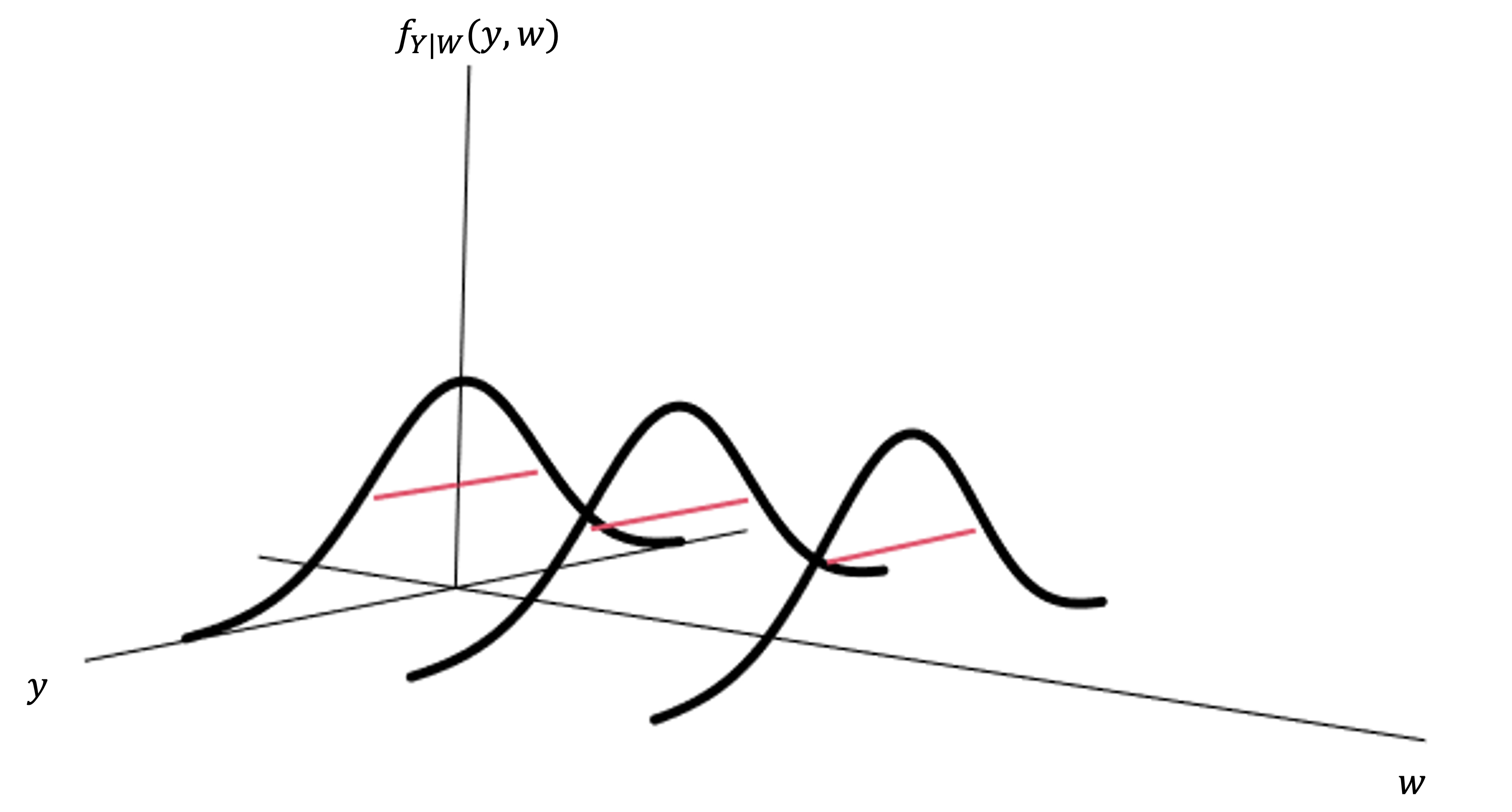
Figure 1: Illustration of the intervals with the largest area under the conditional pdf curves.

Of course, in practice, we are faced with the issue that $f_{Y\mid W,{\bf Z}}({\bf o})$ is unknown. We suggest to compute $f_{Y\mid W,{\bf Z}}^{*}({\bf o},\widehat{\bm{\beta}})$ instead, and then identify the optimal $m(W,{\bf Z},{\bm{\beta}})$ based on $f_{Y\mid W,{\bf Z}}^{*}({\bf o},\widehat{\bm{\beta}})$ using an iterative procedure. Specifically, we select an initial $m(w,{\bf z},\widehat{\bm{\beta}})$, for example $m(w,{\bf z},\widehat{\bm{\beta}})=E^{*}(Y\mid W,{\bf Z},\widehat{\bm{\beta}})$. We then estimate $\zeta$. Based on the estimator $\widehat{\zeta}$ and $f_{Y\mid W,{\bf Z}}^{*}({\bf o},\widehat{\bm{\beta}})$, we identify the optimal $m(w,{\bf z},\widehat{\bm{\beta}})$ as an updated choice of $m(w,{\bf z},\widehat{\bm{\beta}})$. We repeat the procedure of estimating $\zeta$ and updating $m(w,{\bf z},\widehat{\bm{\beta}})$, until $\widehat{\zeta}$ does not decrease sufficiently large for our application purpose.

Clearly, the whole procedure of identifying the optimal $m(w,{\bf z},\widehat{\bm{\beta}})$ relies on the posited model $\eta_{1}^{*}(x,{\bf z},{\bm{\beta}},\zeta)$. If we wish, we can choose several candidate models and retain the result associated with the smallest $\widehat{\zeta}$. We do not need to adjust for multiple testing here, since each probability statement $1-\alpha=\hbox{pr}\{Y_{n+1}\in C(W_{n+1},{\bf Z}_{n+1})\}$, regardless the posited $\eta_{1}^{*}(x,{\bf z})$, is valid.

5 Alternative prediction methods

We now prescribe two alternative ways for prediction in the measurement error models. The first method is a direct approach, where the relation between $Y$ and $X$ is completely bypassed. Instead, one directly inspects the relation between $Y$ and $W,{\bf Z}$ for prediction. The second approach is a naive approach, where one treats $W$ as if it is $X$. In the prediction interval context, we show that both methods are consistent, although they have drawbacks in comparison to the semiparametric method.

5.1 Direct prediction

Because our goal is to predict $Y$ based on $W,{\bf Z}$, which are observed in our data, so a direct approach is to establish the relation between $Y$ and $W,{\bf Z}$ and perform prediction. In this sense, the measurement error issue is completely dismissed. Specifically, in the direct prediction approach, we assume $Y=m(w,{\bf z})+\epsilon$ and we estimate $m(w,{\bf z})$ nonparametrically to form the residuals $r({\bf O})$. We then find the prediction interval by estimating $\zeta$ based on the same relation $\hbox{pr}\{r({\bf O})<\zeta\}=1-\alpha$. In Appendix A.6, we show that in this approach, the efficient influence function for estimating $\zeta$ is

$$\phi_{\rm direct}({\bf O},\zeta)=\frac{(1-\alpha)-I\{r({\bf O},m)<\zeta\}-\epsilon E[\delta\{\zeta-r({\bf O},m)\}\mid W,{\bf Z}]}{E[\delta\{\zeta-r({\bf O})\}]}.$$

We subsequently estimate $\zeta$ via solving $\sum_{i=1}^{n}\phi_{\rm direct}({\bf O}_{i},\zeta)=0$.

5.2 Naive prediction

A naive approach in measurement error models is to treat $W$ as if it were $X$ and perform the standard analysis. While it is known that this will lead to an inconsistent estimator for ${\bm{\beta}}$, this is nevertheless a valid method for prediction interval construction. Specifically, we can estimate ${\bm{\beta}}$ by the usual regression methods, and then form the prediction interval by estimating $\sum_{i=1}^{n}\phi_{\rm naive}({\bf O}_{i},\widehat{\bm{\beta}},\zeta)=0$. In Appendix A.7, we show that the efficient influence function for estimating $\zeta$ is

$$\phi_{\rm naive}({\bf O},{\bm{\beta}},\zeta)$$

$$= \frac{1-\alpha-I\{r({\bf O},{\bm{\beta}})<\zeta\}}{E[\delta\{\zeta-r({\bf O},{\bm{\beta}})\}]}+\epsilon\frac{E[\epsilon I\{r({\bf O},{\bm{\beta}})<\zeta\}\mid W,{\bf Z}]}{E[\delta\{\zeta-r({\bf O},{\bm{\beta}})\}]E(\epsilon^{2}\mid W,{\bf Z})}$$

$$+\epsilon{\bf m}_{\bm{\beta}}^{\prime}(w,{\bf z},{\bm{\beta}})^{\rm T}\left[E\left\{\frac{{\bf m}_{\bm{\beta}}^{\prime}(W,{\bf Z},{\bm{\beta}})^{\otimes 2}}{\hbox{var}(\epsilon^{2}\mid W,{\bf Z})}\right\}\right]^{-1}$$

$$\times E\left(\frac{\delta\{\zeta-r({\bf O},{\bm{\beta}})\}{\partial r({\bf O},{\bm{\beta}})}/{\partial{\bm{\beta}}}}{E[\delta\{\zeta-r({\bf O},{\bm{\beta}})\}]}+\frac{\epsilon I\{r({\bf O},{\bm{\beta}})<\zeta\}{\bf m}_{\bm{\beta}}^{\prime}(W,{\bf Z},{\bm{\beta}})}{E[\delta\{\zeta-r({\bf O},{\bm{\beta}})\}]E(\epsilon^{2}\mid W,{\bf Z})}\right).$$

6 Simulation studies

In our first simulation, we let ${\bf Z}=(1,Z_{1},Z_{2})^{\rm T}$, where $Z_{1}\sim U(0,1)$, $Z_{2}$ is a Bernoulli random variable with probability 0.8 to be one. We generate $X$ from a scaled and shifted beta distribution $X\sim 2\sqrt{3}{\rm Beta}(2,2)-\sqrt{3}$, and set $W=X+U$, where $U\sim N(0,\sigma_{U}^{2})$ with $\sigma_{U}=0.3$. We then generate $Y=m(X,{\bf Z},{\bm{\beta}})+\epsilon$, where $\epsilon\sim N(0,\sigma_{\epsilon}^{2}),\sigma_{\epsilon}=0.1$. Here we experiment with three different mean models:

• $m_{1}(X,{\bf Z},{\bm{\beta}})=(X,X^{2}){\bm{\beta}}_{1}+{\bf Z}^{\rm T}{\bm{\beta}}_{2}$,

• $m_{2}(X,{\bf Z},{\bm{\beta}})=\sin\{(X,X^{2}){\bm{\beta}}_{1}+{\bf Z}^{\rm T}{\bm{\beta}}_{2}\},$

• $m_{3}(X,{\bf Z},{\bm{\beta}})=\exp[-\{(X,X^{2}){\bm{\beta}}_{1}+{\bf Z}^{\rm T}{\bm{\beta}}_{2}\}^{2}]$,

where ${\bm{\beta}}=({\bm{\beta}}_{1}^{\rm T},{\bm{\beta}}_{2}^{\rm T})^{\rm T}=(4,1,1,1,0.5)^{\rm T}$. We simulate the data with sample sizes $n=100$ and $n=500$ respectively.

We implement six methods to perform prediction. In all these methods, we use $\widehat{E}(Y|w,{\bf z})$ to denote the kernel estimator of the conditional mean of $Y$ given $w,{\bf z}$. In addition, in obtaining ${\bf a}(X,{\bf Z},{\bm{\beta}})$ and $a_{1}(X,{\bf Z},{\bm{\beta}},\zeta)$, we use a K-means algorithm to group ${\bf Z}$ to two groups, and adopt the same ${\bf Z}$ in each group.

• m1s: $r({\bf o},{\bm{\beta}})=|y-E^{*}(Y|w,{\bf z},{\bm{\beta}})|$. We use semiparametric method to estimate both ${\bm{\beta}}$ and $\zeta$.

• m1c: $r({\bf o},{\bm{\beta}})=|y-E^{*}(Y|w,{\bf z},{\bm{\beta}})|$. We use semiparametric method to estimate ${\bm{\beta}}$ and conformal prediction to estimate $\zeta$.

• m2s: $r({\bf o},m)=|y-\widehat{E}(Y|w,{\bf z})|$. We use nonparametric method to estimate $m$ and the direct method in Section 5.1 to estimate $\zeta$.

• m2c: $r({\bf o},m)=|y-\widehat{E}(Y|w,{\bf z})|$. We use nonparametric method to estimate $m$ and conformal prediction to estimate $\zeta$.

• m3s: $r({\bf o},{\bm{\beta}})=|y-m(w,{\bf z},{\bm{\beta}})|$. We adopt the naive model $y=m(w,{\bf z},{\bm{\beta}})+\epsilon$ to estimate ${\bm{\beta}}$, and use the native method in Section 5.2 to estimate $\zeta$.

• m3c: $r({\bf o},{\bm{\beta}})=|y-m(w,{\bf z},{\bm{\beta}})|$. We adopt the naive model $y=m(w,{\bf z},{\bm{\beta}})+\epsilon$ to estimate ${\bm{\beta}}$, and use conformal prediction estimate $\zeta$.

In all the implementation of the conformal prediction method, we use the split data approach, where we use half of the data for model estimation and the other half for prediction. We can see that methods m1s and m1c both take into account the model information and the measurement issue, where m1s is our proposed method using semiparametrics to form prediction, while m1c uses conformal prediction approach as a direct competitor. In contrast, methods m2s and m2c completely ignores the model information when forming the “residual” $r(\cdot)$. Both methods use nonparametric approach to perform estimation of the mean function to form residual $r({\bf o},m)$, while m2s subsequently uses semiparametrics to estimate $\zeta$, m2c uses the conformal prediction to do so. Please see Section A.6 in the Appendix for the details on m2s. Note that methods m2s and m2c correspond to the approach by those who hold the view point that measurement error problems do not need to be treated as long as one directly study the relation between the response and the observed variables. Finally, methods m3s and m3c both ignore the presence of the measurement error and treat $W$ as $X$, so are naive methods. m3s and m3c also differ in terms of whether prediction is carried out using semiparametric or conformal prediction, please see Section A.7 for the details in the semiparametric method. In implementing all the methods that require a working model $\eta^{*}$, we adopted the correct distribution in Simulation 1. Specifically, we selected 30 grid points $(x_{j},j=1,\ldots,30)$ on the support of $X$, and let the weights be $\eta^{*}(x_{i})=\sum_{j=1}^{30}I(x_{i}=x_{j})\eta_{{\bf x}}(x_{j})/\sum_{j=1}^{30}\eta_{{\bf x}}(x_{j})$, where $\eta_{{\bf x}}$ is the density of the scaled and shifted ${\rm Beta}(2,2)$ distribution.

Based on the $n$ estimated 90% prediction intervals, we computed the coverage probability (CP) and the average length (LPI), and provided the box-plots from the 100 simulations in Figures 2 and 3. Further, in Table 1, we present the mean and standard deviation of the 100 CPs, as well as the mean and standard deviation of the 100 prediction interval lengths. We can see that in general, all methods provide coverage close to the nominal level 90%, hence are all consistent.

In most cases, the prediction intervals of all the consistent estimators tend to be the shortest in m1s and m1c, where we used the model information. They are the largest in m3c, where the measurement error issue is naively ignored, and are in the middle for m2s and m2c, when the model information is completely ignored. Within each of the three method classes, the semiparametric approach leads to better performance, in that the box is generally narrower, reflecting smaller variability. Among all six methods, it is quite clear that m1s has the best performance, in terms of its good coverage, short length and small variabilities. The observed small variability agrees with our theory, because when the working model is correct, under the same residual form, the semiparametric method provides the most efficient estimation of the prediction interval. Further, as we have pointed out, among the three semiparametric methods m1s, m2s, m3s, we can see that m1s has the best performance in general. This indicates that it is beneficial to make use of the model information and to take into account the measurement error issue.

We also conducted a simulation 2, where we adopted a misspecified model for the distribution of $X$. In this simulation, we generated $X$ via $X\sim N(-1,1)$, while we choose $\eta^{*}$ to be a discrete uniform distribution function with 30 positive masses on $(\widehat{\mu}_{x}-3\widehat{\sigma}_{x},\widehat{\mu}_{x}+3\widehat{\sigma}_{x})$. Here $\widehat{\mu}_{x}$ is the estimated mean of $X$ calculated by the sample average of $W$, and $\widehat{\sigma}_{x}^{2}$ is the estimated variance of $X$ calculated by the sample variance of $W$ minus $\sigma_{U}^{2}$. All other aspects of the simulation are identical to those in Simulation 1. The results are in Table 2. Similar conclusions can be drawn as in Simulation 1. Note that here because the distribution of $X$ is misspecified, there is no theoretical guarantee that the prediction interval is optimally estimated. However, we observe smaller variability throughout in comparison to the corresponding conformal approach.

We also performed an additional simulation study to investigate the performance when the model error distribution is misspecified. The methods are very robust, while we provide the simulation details in Appendix A.8.

Table 1: Simulation 1, true distribution for $X$. The average and standard deviation of the coverage probabilities (CP (SD)), and the average and standard deviation of the lengths (LPI (SD)) of the estimated 90% prediction intervals.

	m1s	m1c	m2s	m2c	m3s	m3c
	$n=100$
	model 1
CP (SD)	0.9 (0.021)	0.903 (0.042)	0.904 (0.035)	0.902 (0.046)	0.904 (0.022)	0.902 (0.041)
LPI (SD)	4.024 (0.241)	4.102 (0.596)	4.38 (0.457)	4.796 (0.945)	4.111 (0.275)	4.271 (0.607)
	model 2
CP (SD)	0.889 (0.02)	0.904 (0.041)	0.88 (0.046)	0.896 (0.042)	0.906 (0.024)	0.905 (0.044)
LPI (SD)	1.949 (0.095)	2.057 (0.231)	2.011 (0.202)	2.207 (0.266)	2.633 (0.197)	2.679 (0.402)
	model 3
CP (SD)	0.895 (0.022)	0.897 (0.051)	0.902 (0.036)	0.9 (0.044)	0.898 (0.024)	0.899 (0.046)
LPI (SD)	0.862 (0.079)	0.881 (0.146)	0.959 (0.101)	1.035 (0.175)	1.076 (0.094)	1.133 (0.259)
	$n=500$
	model 1
CP (SD)	0.896 (0.016)	0.9 (0.023)	0.904 (0.017)	0.9 (0.022)	0.899 (0.015)	0.9 (0.023)
LPI (SD)	3.974 (0.106)	4.015 (0.29)	4.054 (0.22)	4.065 (0.309)	3.941 (0.187)	4.017 (0.301)
	model 2
CP (SD)	0.894 (0.013)	0.9 (0.019)	0.895 (0.019)	0.899 (0.02)	0.903 (0.019)	0.901 (0.019)
LPI (SD)	1.901 (0.039)	2.022 (0.105)	2.026 (0.096)	2.041 (0.104)	2.511 (0.138)	2.603 (0.187)
	model 3
CP (SD)	0.893 (0.016)	0.899 (0.022)	0.899 (0.019)	0.902 (0.021)	0.899 (0.017)	0.899 (0.021)
LPI (SD)	0.852 (0.042)	0.873 (0.064)	0.888 (0.063)	0.906 (0.078)	1.001 (0.081)	1.044 (0.137)

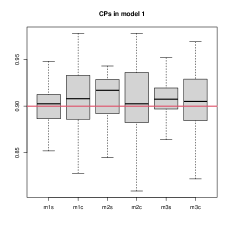
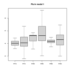
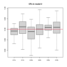
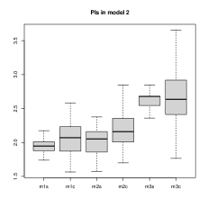
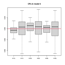
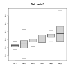
Figure 2: Simulation 1: Boxplots of the 90% coverage probability (CP) and prediction interval length (PI) of the estimated prediction interval in the three models using the six methods. $n=100$.

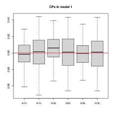
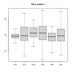
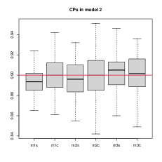
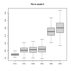
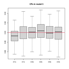
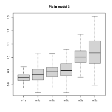
Figure 3: Simulation 1: Boxplots of the 90% coverage probability (CP) and prediction interval length (PI) of the estimated prediction interval in the three models using the six methods. $n=500$.

Table 2: Simulation 2, misspecified distribution for $X$. The average and standard deviation of the coverage probabilities (CP (SD)), and the average and standard deviation of the lengths (LPI (SD)) of the estimated 90% prediction intervals.

	m1s	m1c	m2s	m2c	m3s	m3c
	$n=100$
	model 1
CP (SD)	0.893 (0.017)	0.898 (0.038)	0.915 (0.026)	0.897 (0.038)	0.908 (0.019)	0.904 (0.04)
LPI (SD)	2.91 (0.215)	3.087 (0.593)	3.407 (0.343)	3.673 (0.962)	2.843 (0.218)	2.952 (0.534)
	model 2
CP (SD)	0.895 (0.019)	0.91 (0.036)	0.906 (0.032)	0.907 (0.041)	0.913 (0.02)	0.909 (0.034)
LPI (SD)	1.544 (0.086)	1.66 (0.215)	1.818 (0.192)	1.975 (0.372)	1.98 (0.201)	2.052 (0.343)
	model 3
CP (SD)	0.907 (0.021)	0.906 (0.038)	0.905 (0.041)	0.904 (0.039)	0.904 (0.029)	0.902 (0.039)
LPI (SD)	0.907 (0.056)	0.92 (0.125)	1.012 (0.12)	1.091 (0.164)	1.141 (0.085)	1.185 (0.241)
	$n=500$
	model 1
CP (SD)	0.893 (0.013)	0.898 (0.021)	0.894 (0.02)	0.898 (0.021)	0.897 (0.014)	0.896 (0.022)
LPI (SD)	2.79 (0.11)	2.907 (0.293)	2.68 (0.208)	2.802 (0.28)	2.618 (0.16)	2.636 (0.241)
	model 2
CP (SD)	0.901 (0.013)	0.898 (0.023)	0.891 (0.022)	0.897 (0.023)	0.902 (0.016)	0.898 (0.022)
LPI (SD)	1.613 (0.042)	1.607 (0.103)	1.555 (0.129)	1.632 (0.125)	1.771 (0.145)	1.893 (0.253)
	model 3
CP (SD)	0.9 (0.012)	0.897 (0.024)	0.896 (0.02)	0.898 (0.024)	0.897 (0.022)	0.897 (0.021)
LPI (SD)	0.884 (0.027)	0.887 (0.067)	0.883 (0.059)	0.916 (0.067)	1.022 (0.086)	1.054 (0.131)

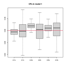
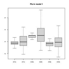
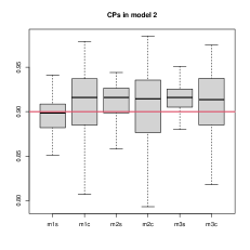
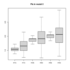
Figure 4: Simulation 2: Boxplots of the 90% coverage probability (CP) and prediction interval length (PI) of the estimated prediction interval in the three models using the six methods. $n=100$.

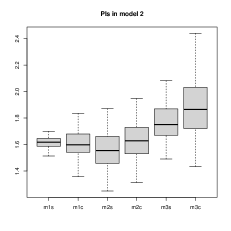
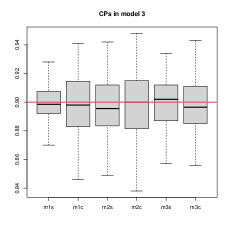
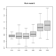
Figure 5: Simulation 2: Boxplots of the 90% coverage probability (CP) and prediction interval length (PI) of the estimated prediction interval in the three models using the six methods. $n=500$.

7 Real data analysis

Alzheimer’s disease (AD) is the most common cause of dementia and is characterized by accumulation of amyloid-$\beta$ ($A\beta$) plaques in the earliest phase of the disease (Masters & Bateman, 2015; Scheltens et al., 2016). Two established methods for detecting the presence of $A\beta$ pathology are reduced concentrations of $A\beta 1-42$ ($A\beta 42$) in cerebrospinal fluid (CSF) and increased retention of $A\beta$ positron emission tomography (PET) tracers (Mattsson et al., 2017). It is often assumed that CSF $A\beta 42$ and $A\beta$ PET can be used interchangeably, because there are mounting evidences showing that PET and CSF biomarkers are strongly associated (Schipke et al., 2017; Leuzy et al., 2016; Palmqvist et al., 2015). It is natural to ask how accurate it would be if we use one marker, for example $A\beta$ PET to predict the other. Ideally, if one perfectly predicts the other, patients will no longer need to take multiple examinations, which reduces the chance of side effect and lowers patients’ psychological stress. However, prediction based on neuroimage data is challenging because neuroimage data are often subject to measurement errors resulting from the data acquisition and processing steps.

We utilize the prediction interval methods m1s–m3c discussed in Section 6 to study the performance of using the standardized uptake value ratio (SUVR) of florbetapir (radiotracer) from the $A\beta$ PET to predict the $A\beta 42$ from CSF. We download the preprocessed CSF (Shaw et al., 2016) and florbetapir PET (Landau et al., 2021) data from the Alzheimer’s Disease Neuroimaging Initiative (ADNI) phase 2/Go study, from which we obtain a subsample with $A\beta 42$ values from the CSF tests that were taken within 30 days of the PET scans. Furthermore, we only retain the healthy subjects and the subjects with Alzheimer’s disease who had their diagnoses within 30 days of the CSF tests. After removing missing data, we obtain 669 subjects (48.5% female) with an average age of 74.5 years, where 388 are classified as CSF negative subjects at the risk of cognitive impairment, and among which 220 are subjects with AD. Let $Y$ be the logarithm of $A\beta 42$ from CSF, $W$ be the SUVR from PET, ${\bf Z}=\{1,{\rm gender},{\rm log}({\rm age})\}^{\rm T}$. The scatter plot in the left panel of Figure 6 indicates an approximate quadratic relationship between $Y$ and $W$, therefore we assume $m(X,{\bf Z},{\bm{\beta}})=(X,X^{2}){\bm{\beta}}_{1}+{\bf Z}^{\rm T}{\bm{\beta}}_{2}$, where $X$ is the underlying error free covariate. The box plots in the right panel of Figure 6 indicate that there is a significant difference in CSF values between healthy (199.748 $\pm$ 51.30) and AD groups (135.465 $\pm$ 37.57), with the p-value from a student t-test to be less than 0.0001.

We randomly sample two thirds of the subjects to construct the prediction interval and evaluate the coverage probability on the remaining one third. We repeat the above cross validation process 100 times to compare the performance of m1s–m3c. In m1s and m1c, we choose $\eta^{*}$ to be a normal probability density function and assign 30 positive masses evenly spaced on $(\widehat{\mu}_{x}-r_{1}\widehat{\sigma}_{x},\widehat{\mu}_{x}+r_{2}\widehat{\sigma}_{x})$. Here $\widehat{\mu}_{x}$ is the estimated mean of $X$ calculated by the sample average of $W$, and $\widehat{\sigma}_{x}^{2}$ is the estimated variance of $X$ calculated by the sample variance of $W$ minus $\sigma_{U}^{2}$. We set $\sigma_{U}$ to be 10% of the standard deviation of $W$ based on empirical knowledge and experience. Furthermore, following Romano et al. (2019) we calibrate the tuning parameters $\sigma_{\epsilon},r_{1},r_{2}$ (in m1s, m1c) and the kernel bandwidths (in m2s, m2c) to allow the coverage probabilities in the test samples to achieve the nominal 90% level on average in the cross validation. Figure 7 indicates that all six methods are consistent, which yield the coverage probabilities close to 90%, while the semiparametric methods generally have much smaller variations in CP and PI.

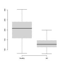
Figure 6: Left: The scatterplots of CSF $A\beta$ and SUVR from amyloid PET. Right: The distribution of CSF values in healthy and AD subjects.

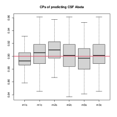
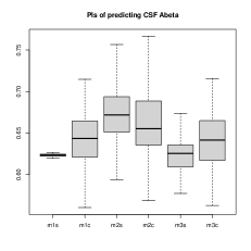
Figure 7: Boxplots of the 90% coverage probability (CP) and prediction interval length (PI) of the estimated prediction interval using the six methods m1s–m3c over 100 cross validations.

To illustrate how to use the prediction interval in practice, we propose two strategies to predict whether a subject has AD or is healthy based on his/her SUVR value. In strategy 1 (interval strategy), we categorize a subject to be an AD patient if the lower bound of his/her 90% PI is less than the estimated mean of ${\rm log}(A\beta 42)$ in the AD group. In strategy 2 (mean strategy), we categorize a subject to AD if the estimated conditional mean of $Y$ given $W$ is less than the 90% upper confidence bound of mean ${\rm log}(A\beta 42)$ in the AD group. Here, the specific form of the conditional mean for m1s, m1c is $E^{*}(Y|w,{\bf z},\widehat{\bm{\beta}})$, for m2s, m2c is $\widehat{E}(Y|w,{\bf z})$, and for m3s, m3c is $m(w,{\bf z},\widehat{\bm{\beta}})$ as described in the definitions of these methods in Section 6.

We show the area under the receiver operating characteristic (AUC) curve of the two prediction strategies in Figure 8. As shown in Figure 8, the interval strategy outperforms the mean strategy in all methods. Furthermore, in the interval strategy, the AUCs from the semiparametric methods (m1s, m2s and m3s) have smaller variations than those from their conformal counterparts (m1c, m2c and m3c) as shown in the upper part of Table 3, which likely attributes to the fact that the semiparametric methods have smaller variations in PI. Moreover, by considering the measurement errors, the combination of the interval strategy and m1s method achieves the smallest variability in AUC. It is worth mentioning that the interval strategy also outperforms the standard clinical practice of using CSF positive/negative to diagnose AD as shown in Figure 8.

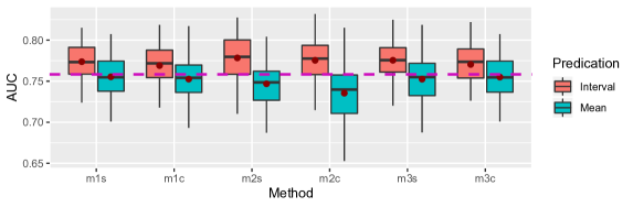
Figure 8: Boxplots over 100 cross validation of AUC from interval and mean strategies of predicting CSF $A\beta$ postive and negative samples. The dash-line represents the AUC of using CSF positive/negative to classify AD and healthy subject (AUC$=0.7583$).

Table 3: The mean and standard deviation over 100 cross validation of AUC from interval and mean strategies of predicting CSF $A\beta$ postive and negative samples.

	m1s	m1c	m2s	m2c	m3s	m3c
	Interval strategy
Mean	0.7738	0.7691	0.7784	0.7755	0.7755	0.7704
Standard deviation	0.0204	0.0238	0.0247	0.0252	0.0224	0.0236
	Mean strategy
Mean	0.7554	0.7526	0.7468	0.7354	0.7525	0.7550
Standard deviation	0.0259	0.0291	0.0279	0.0321	0.0283	0.0261

8 Discussion

Many interesting problems are worth further research in the prediction issue for measurement error models. We highlight some here.

We have used the method in Tsiatis & Ma (2004) as the estimator due to its generality and root-$n$ rate. Other estimation methods can certainly be used. When the original model is nonparametric and semiparametric, various other methods exist based on deconvolution or Sieve (Chen et al., 2008, 2009; Carroll et al., 2010), and some even handle high dimensional covariates (Jiang & Ma, 2022; Jiang et al., 2023, 2024). See Li & Ma (2024) for a recent review. These methods can also be incorporated with the prediction procedures proposed here. When different estimators are combined with the prediction interval construction, their subsequent analysis will be different and some could be challenging.

As we have mentioned, more general choice of the conformal score $r({\bf o},{\bm{\beta}})$ is possible beyond the form $|y-m(w,{\bf z},{\bm{\beta}})|$. Under the general conformal score $r({\bf o},{\bm{\beta}})$, one can also ask the question: what choice of the conformal score will lead to the smallest prediction set $C(W_{n+1},{\bf Z}_{n+1})$, where it satisfies $\hbox{pr}\{Y_{n+1}\in C(W_{n+1},{\bf Z}_{n+1})\}=\hbox{pr}\{r({\bf o},{\bm{\beta}})<\zeta\}=1-\alpha$. Note that as soon as the functional form of $r({\bf o},{\bm{\beta}})$ is chosen, different estimators of ${\bm{\beta}}$ and $\zeta$ only affect the estimated version of $C(W_{n+1},{\bf Z}_{n+1})$. So identifying the smallest conformal set $C(W_{n+1},{\bf Z}_{n+1})$ is not a statistical problem, but a mathematical problem, which involves inverting $r({\bf O}_{n+1},{\bm{\beta}})<\zeta$ to obtain $C(W_{n+1},{\bf Z}_{n+1})$ and finding the optimal $r$ which yields a smallest $C(W_{n+1},{\bf Z}_{n+1})$ under a predefined measure. Unfortunately, this is a very difficult question to answer in general. To see the potential difficulties, as an example, if we have set $r({\bf o},{\bm{\beta}})=-{\rm log}f_{Y\mid W,{\bf Z}}^{*}({\bf o},{\bm{\beta}})$, then we get

$$1-\alpha = \hbox{pr}\{-{\rm log}f_{Y\mid W,{\bf Z}}^{*}({\bf O}_{n+1},{\bm{\beta}})<\zeta\}$$

$$= E[\hbox{pr}\{-{\rm log}f_{Y\mid W,{\bf Z}}^{*}({\bf O}_{n+1},{\bm{\beta}})<\zeta\mid W_{n+1},{\bf Z}_{n+1}\}].$$

From here, we cannot further conclude that $\zeta$ is directly linked to the size of $C(W_{n+1},{\bf Z}_{n+1})$, unless we assume special features of $f_{Y\mid W,{\bf Z}}^{*}({\bf o},{\bm{\beta}})$ as a function of $y$. Thus we suspect this problem has to be studied case-by-case in specific concrete models.

Lastly, we comment on the original issue of predicting a single response $Y_{n+1}$ given $W_{n+1},{\bf Z}_{n+1}$. Indeed, at any $m(w,{\bf z},{\bm{\beta}})$, we can estimate the prediction interval associated with any $\eta_{1}^{*}(x,{\bf z})$. Thus, we can use the smallest non-empty intersection of any of these intervals as a most aggressive prediction interval. Now if we consider an increasing series of $\alpha$ values that approach 1, we can obtain a series of intervals, which approximates the single prediction value. This of course does not necessarily lead to a single value. In fact, we cannot guarantee that the interval length will approach zero.

Appendix

A.1 Proof of Proposition 1: the efficient influence function for $\zeta$

Let the dimension of ${\bm{\beta}}$ be $d_{\bm{\beta}}$. Let $f_{X\mid{\bf Z}}(x,{\bf z},\bm{\gamma}_{1}),f_{\bf Z}({\bf z},\bm{\gamma}_{2})$ be parametric sub-models of $\eta_{1}(x,{\bf z}),\eta_{2}({\bf z})$. We can easily see that the score functions are

$${\bf S}_{{\bm{\beta}}}({\bf o},{\bm{\beta}}) \equiv \frac{\partial{\rm log}\int\eta_{1}(x,{\bf z})\eta_{2}({\bf z})f_{W\mid X,{\bf Z}}(w,x,{\bf z})f_{Y\mid X,{\bf Z}}(y,x,{\bf z},{\bm{\beta}})dx}{\partial{\bm{\beta}}}$$

$$= \frac{\int{\partial{\rm log}f_{Y\mid X,{\bf Z}}(y,x,{\bf z},{\bm{\beta}})}/{\partial{\bm{\beta}}}\eta_{1}({\bf x},{\bf z})\eta_{2}({\bf z})f_{W\mid X,{\bf Z}}(w,x,{\bf z})f_{Y\mid X,{\bf Z}}(y,x,{\bf z},{\bm{\beta}})dx}{\int\eta_{2}({\bf z})\eta_{1}(x,{\bf z})f_{W\mid X,{\bf Z}}(w,x,{\bf z})f_{Y\mid X,{\bf Z}}(y,x,{\bf z},{\bm{\beta}})dx}$$

$$= E\left\{\frac{\partial{\rm log}f_{Y\mid X,{\bf Z}}(y,X,{\bf z},{\bm{\beta}})}{\partial{\bm{\beta}}}\mid{\bf O}={\bf o}\right\},$$

$${\bf S}_{\bm{\gamma}_{1}}({\bf o},{\bm{\beta}}) \equiv \frac{\partial{\rm log}\int\eta_{2}({\bf z})f_{X\mid{\bf Z}}(x,{\bf z},\bm{\gamma}_{1})f_{W\mid X,{\bf Z}}(w,x,{\bf z})f_{Y\mid X,{\bf Z}}(y,x,{\bf z},{\bm{\beta}})dx}{\partial\bm{\gamma}_{1}}$$

$$= \frac{\int{\partial{\rm log}f_{X\mid{\bf Z}}(x,{\bf z},\bm{\gamma}_{1})}/{\partial\bm{\gamma}_{1}}\eta_{2}({\bf z})f_{X\mid{\bf Z}}(x,{\bf z},\bm{\gamma}_{1})f_{W\mid X,{\bf Z}}(w,x,{\bf z})f_{Y\mid X,{\bf Z}}(y,x,{\bf z},{\bm{\beta}})dx}{\int\eta_{2}({\bf z})\eta_{1}(x,{\bf z})f_{W\mid X,{\bf Z}}(w,x,{\bf z})f_{Y\mid X,{\bf Z}}(y,x,{\bf z},{\bm{\beta}})dx}$$

$$= E\left\{\frac{\partial{\rm log}f_{X\mid{\bf Z}}(X,{\bf z},\bm{\gamma}_{1})}{\partial\bm{\gamma}_{1}}\mid Y=y,W=w,{\bf Z}={\bf z}\right\},$$

$${\bf S}_{\bm{\gamma}_{2}}({\bf z},\bm{\gamma}_{2}) \equiv \frac{\partial{\rm log}\int\eta_{1}({\bf x},{\bf z})f_{\bf Z}({\bf z},\bm{\gamma}_{2})f_{W\mid X,{\bf Z}}(w,x,{\bf z})f_{Y\mid X,{\bf Z}}(y,x,{\bf z},{\bm{\beta}})dx}{\partial\bm{\gamma}_{2}}$$

$$= \frac{\partial{\rm log}f_{\bf Z}({\bf z},\bm{\gamma}_{2})}{\partial\bm{\gamma}_{2}}.$$

Thus, the tangent space ${\cal T}$, which is the span of all the score functions derived above associated with all the possible parametric submodels, is ${\cal T}=\Lambda_{\bm{\beta}}+(\Lambda_{1}\oplus\Lambda_{2})=\Lambda_{\rm eff}\oplus\Lambda_{1}\oplus\Lambda_{2}$, where

$$\Lambda_{\bm{\beta}} = \left\{{\bf c}^{\rm T}{\bf S}_{\bm{\beta}}({\bf o},{\bm{\beta}}):{\bf c}\in\mathbb{R}^{d_{\bm{\beta}}}\right\}$$

$$\Lambda_{1} = \left[E\{a(X,{\bf z})\mid{\bf O}={\bf o}\}:E\{a(X,{\bf z})\mid{\bf z}\}=0\right]$$

$$\Lambda_{2} = [a({\bf z}):E\{a({\bf Z})\}=0],$$

$$\Lambda_{\rm eff} = \left\{{\bf c}^{\rm T}{\bf S}_{\rm eff}({\bf o},{\bm{\beta}}):{\bf c}\in\mathbb{R}^{d_{\bm{\beta}}}\right\}.$$

Here, we rewrite $\Lambda_{\bm{\beta}}+(\Lambda_{1}\oplus\Lambda_{2})$ into $\Lambda_{\rm eff}\oplus\Lambda_{1}\oplus\Lambda_{2}$ to ease the utility of ${\cal T}$ later when we compute the efficient influence function.

Next, we compute the derivatives of $\zeta$ with respect to the parameters ${\bm{\beta}},\bm{\gamma}_{1},\bm{\gamma}_{2}$ associated with an arbitrary parametric submodel. Consider

$$1-\alpha = \hbox{pr}\{r({\bf O},{\bm{\beta}})<\zeta({\bm{\beta}},\eta_{1},\eta_{2})\}$$

$$= \int_{{\bf o}:r({\bf o},{\bm{\beta}})<\zeta({\bm{\beta}},\eta_{1},\eta_{2})}f_{\bf O}({\bf o},{\bm{\beta}},\eta_{1},\eta_{2})d{\bf o}$$

$$= \int_{{\bf o}:r({\bf o},{\bm{\beta}})<\zeta({\bm{\beta}},\eta_{1},\eta_{2})}\eta_{1}(x,{\bf z})\eta_{2}({\bf z})f_{W\mid X,{\bf Z}}(w,x,{\bf z})f_{Y\mid X,{\bf Z}}(y,x,{\bf z},{\bm{\beta}})d\mu(x,{\bf o}),$$

where we write $\zeta$ as $\zeta({\bm{\beta}},\eta_{1},\eta_{2})$ to emphasize that $\zeta$ is a functional of ${\bm{\beta}},\eta_{1},\eta_{2}$. Taking derivative with respect to ${\bm{\beta}}$ leads to

$${\bf 0} = \int I\{r({\bf o},{\bm{\beta}})<\zeta({\bm{\beta}},\eta_{1},\eta_{2})\}{\bf S}_{\bm{\beta}}(y,w,{\bf z},{\bm{\beta}},\eta_{1},\eta_{2})f_{\bf O}({\bf o},{\bm{\beta}},\eta_{1},\eta_{2})d{\bf o}$$

$$+\int\delta\{\zeta({\bm{\beta}},\eta_{1},\eta_{2})-r({\bf o},{\bm{\beta}})\}\left\{\frac{\partial\zeta({\bm{\beta}},\eta_{1},\eta_{2})}{\partial{\bm{\beta}}}-\frac{\partial r({\bf o},{\bm{\beta}})}{\partial{\bm{\beta}}}\right\}f_{\bf O}({\bf o},{\bm{\beta}},\eta_{1},\eta_{2})d{\bf o}$$

$$= E\left[I\{r({\bf O},{\bm{\beta}})<\zeta({\bm{\beta}},\eta_{1},\eta_{2})\}{\bf S}_{\bm{\beta}}({\bf O},{\bm{\beta}},\eta_{1},\eta_{2})\right]$$

$$+\frac{\partial\zeta({\bm{\beta}},\eta_{1},\eta_{2})}{\partial{\bm{\beta}}}\int\delta\{\zeta({\bm{\beta}},\eta_{1},\eta_{2})-r({\bf o},{\bm{\beta}})\}f_{\bf O}({\bf o},{\bm{\beta}},\eta_{1},\eta_{2})d{\bf o}$$

$$-\int\delta\{\zeta({\bm{\beta}},\eta_{1},\eta_{2})-r({\bf o},{\bm{\beta}})\}\frac{\partial r({\bf o},{\bm{\beta}})}{\partial{\bm{\beta}}}f_{\bf O}({\bf o},{\bm{\beta}},\eta_{1},\eta_{2})d{\bf o},$$

hence

$$\frac{\partial\zeta({\bm{\beta}},\eta_{1},\eta_{2})}{\partial{\bm{\beta}}} = \frac{\int\delta\{\zeta-r({\bf o},{\bm{\beta}})\}\frac{\partial r({\bf o},{\bm{\beta}})}{\partial{\bm{\beta}}}f_{\bf O}({\bf o},{\bm{\beta}},\eta_{1},\eta_{2})d{\bf o}}{\int\delta\{\zeta({\bm{\beta}},\eta_{1},\eta_{2})-r({\bf o},{\bm{\beta}})\}f_{\bf O}({\bf o},{\bm{\beta}},\eta_{1},\eta_{2})d{\bf o}}$$

$$-\frac{E\left[I\{r({\bf O},{\bm{\beta}})<\zeta\}{\bf S}_{\bm{\beta}}({\bf O},{\bm{\beta}},\eta_{1},\eta_{2})\right]}{\int\delta\{\zeta({\bm{\beta}},\eta_{1},\eta_{2})-r({\bf o},{\bm{\beta}})\}f_{\bf O}({\bf o},{\bm{\beta}},\eta_{1},\eta_{2})d{\bf o}}$$

$$= \frac{E[\delta\{\zeta-r({\bf O},{\bm{\beta}})\}\frac{\partial r({\bf O},{\bm{\beta}})}{\partial{\bm{\beta}}}]-E[I\{r({\bf O},{\bm{\beta}})<\zeta\}{\bf S}_{\bm{\beta}}({\bf O},{\bm{\beta}},\eta_{1},\eta_{2})]}{E[\delta\{\zeta-r({\bf O},{\bm{\beta}})\}]}.$$

Similarly, replacing $\eta_{1}$ with its parametric submodel, and taking derivative with respect to $\bm{\gamma}_{1}$, we have

$${\bf 0} = \int I\{r({\bf o},{\bm{\beta}})<\zeta({\bm{\beta}},\bm{\gamma}_{1},\eta_{2})\}{\bf S}_{\bm{\gamma}_{1}}({\bf o},{\bm{\beta}},\bm{\gamma}_{1},\eta_{2})f_{\bf O}({\bf o},{\bm{\beta}},\bm{\gamma}_{1},\eta_{2})d{\bf o}$$

$$+\int\delta\{\zeta({\bm{\beta}},\bm{\gamma}_{1},\eta_{2})-r({\bf o},{\bm{\beta}})\}\frac{\partial\zeta({\bm{\beta}},\bm{\gamma}_{1},\eta_{2})}{\partial\bm{\gamma}_{1}}f_{\bf O}({\bf o},{\bm{\beta}},\bm{\gamma}_{1},\eta_{2})d{\bf o}$$

$$= E\left[I\{r({\bf O},{\bm{\beta}})<\zeta\}{\bf S}_{\bm{\gamma}_{1}}({\bf O},{\bm{\beta}},\bm{\gamma}_{1},\eta_{2})\right]+\frac{\partial\zeta({\bm{\beta}},\bm{\gamma}_{1},\eta_{2})}{\partial\bm{\gamma}_{1}}\int\delta\{\zeta-r({\bf o},{\bm{\beta}})\}f_{\bf O}({\bf o},{\bm{\beta}},\bm{\gamma}_{1},\eta_{2})d{\bf o},$$

hence

$$\frac{\partial\zeta({\bm{\beta}},\bm{\gamma}_{1},\eta_{2})}{\partial\bm{\gamma}_{1}}=-\frac{E[I\{r({\bf O},{\bm{\beta}})<\zeta\}{\bf S}_{\bm{\gamma}_{1}}({\bf O},{\bm{\beta}},\bm{\gamma}_{1},\eta_{2})]}{E[\delta\{\zeta-r({\bf O},{\bm{\beta}})\}]}.$$

Finally, replacing $\eta_{2}$ with its parametric submodel, and taking derivative with respect to $\bm{\gamma}_{2}$, we get

$${\bf 0} = \int I\{r({\bf o},{\bm{\beta}})<\zeta({\bm{\beta}},\eta_{1},\bm{\gamma}_{2})\}{\bf S}_{\bm{\gamma}_{2}}({\bf z},\bm{\gamma}_{2})f_{\bf O}({\bf o},{\bm{\beta}},\eta_{1},\bm{\gamma}_{2})d{\bf o}$$

$$+\int\delta\{\zeta({\bm{\beta}},\eta_{1},\bm{\gamma}_{2})-r({\bf o},{\bm{\beta}})\}\left\{\frac{\partial\zeta({\bm{\beta}},\eta_{1},\bm{\gamma}_{2})}{\partial\bm{\gamma}_{2}}-\frac{\partial r({\bf o},{\bm{\beta}})}{\partial\bm{\gamma}_{2}}\right\}f_{\bf O}({\bf o},{\bm{\beta}},\eta_{1},\bm{\gamma}_{2})d{\bf o}$$

$$= E\left[I\{r({\bf O},{\bm{\beta}})<\zeta\}{\bf S}_{\bm{\gamma}_{2}}({\bf Z},\bm{\gamma}_{2})\right]+\frac{\partial\zeta({\bm{\beta}},\eta_{1},\bm{\gamma}_{2})}{\partial\bm{\gamma}_{2}}\int\delta\{\zeta-r({\bf o},{\bm{\beta}})\}f_{\bf O}({\bf o},{\bm{\beta}},\eta_{1},\bm{\gamma}_{2})d{\bf o},$$

hence

$$\frac{\partial\zeta({\bm{\beta}},\eta_{1},\bm{\gamma}_{2})}{\partial\bm{\gamma}_{2}}=\frac{-E[I\{r({\bf O},{\bm{\beta}})<\zeta\}{\bf S}_{\bm{\gamma}_{2}}({\bf Z},\bm{\gamma}_{2})]}{E[\delta\{\zeta-r({\bf O},{\bm{\beta}})\}]}.$$

We are now ready to characterize te efficient influence function. Let $\phi({\bf o},{\bm{\beta}},\zeta)$ be the efficient influence function for estimating $\zeta$. An efficient influence function much belong to ${\cal T}$, hence it has the form $\phi({\bf o},{\bm{\beta}},\zeta)={\bf c}^{\rm T}{\bf S}_{\rm eff}({\bf o},{\bm{\beta}})+E\{\widetilde{a}_{1}(X,{\bf z},{\bm{\beta}},\zeta)\mid{\bf O}={\bf o}\}+a_{2}({\bf z})$, where $E\{\widetilde{a}_{1}(X,{\bf z},{\bm{\beta}},\zeta)\mid{\bf z})=0$ and $E\{a_{2}({\bf Z})\}=0$. In addition, at the true parameter values, any influence function, including the efficient influence function $\phi({\bf o},{\bm{\beta}},\zeta)$, must satisfy

$$\frac{\partial\zeta({\bm{\beta}},\eta_{1},\eta_{2})}{\partial{\bm{\beta}}} = E\{\phi({\bf O},{\bm{\beta}},\zeta){\bf S}_{\bm{\beta}}({\bf O})\},$$

$$\frac{\partial\zeta({\bm{\beta}},\bm{\gamma}_{1},\eta_{2})}{\partial\bm{\gamma}_{1}} = E\{\phi({\bf O},{\bm{\beta}},\zeta){\bf S}_{\bm{\gamma}_{1}}({\bf O})\},$$

$$\frac{\partial\zeta({\bm{\beta}},\eta_{1},\bm{\gamma}_{2})}{\partial\bm{\gamma}_{2}} = E\{\phi({\bf O},{\bm{\beta}},\zeta){\bf S}_{\bm{\gamma}_{2}}({\bf Z})\}.$$

This implies that ${\bf c},\widetilde{a}_{1}(x,{\bf z},{\bm{\beta}},\zeta),a_{2}({\bf z})$ must satisfy

$$\frac{E[\delta\{\zeta-r({\bf O},{\bm{\beta}})\}{\partial r({\bf O},{\bm{\beta}})}/{\partial{\bm{\beta}}}]-E[I\{r({\bf O},{\bm{\beta}})<\zeta\}{\bf S}_{\bm{\beta}}({\bf O},{\bm{\beta}},\eta_{1},\eta_{2})]}{E[\delta\{\zeta-r({\bf O},{\bm{\beta}})\}]}$$

$$= E\left\{[{\bf c}^{\rm T}{\bf S}_{\rm eff}({\bf O})+E\{\widetilde{a}_{1}(X,{\bf Z},{\bm{\beta}},\zeta)\mid{\bf O}\}+a_{2}({\bf Z})][{\bf S}_{\rm eff}({\bf O})+E\{{\bf a}(X,{\bf Z},{\bm{\beta}})\mid{\bf O}\}]\right\}$$

$$= E\left\{[{\bf c}^{\rm T}{\bf S}_{\rm eff}({\bf O})+E\{\widetilde{a}_{1}(X,{\bf Z},{\bm{\beta}},\zeta)\mid{\bf O}\}][{\bf S}_{\rm eff}({\bf O})+E\{{\bf a}(X,{\bf Z},{\bm{\beta}})\mid{\bf O}\}]\right\}$$

$$= E\left\{{\bf S}_{\rm eff}({\bf O}){\bf S}_{\rm eff}^{\rm T}({\bf O})\right\}{\bf c}+E\left[E\{\widetilde{a}_{1}(X,{\bf Z},{\bm{\beta}},\zeta)\mid{\bf O}\}E\{{\bf a}(X,{\bf Z},{\bm{\beta}})\mid{\bf O}\}\right],$$

$$\frac{-E[I\{r({\bf O},{\bm{\beta}})<\zeta\}{\bf S}_{\bm{\gamma}_{1}}({\bf O},{\bm{\beta}},\bm{\gamma}_{1},\eta_{2})]}{E[\delta\{\zeta-r({\bf O},{\bm{\beta}})\}]}$$

$$= E\left([{\bf c}^{\rm T}{\bf S}_{\rm eff}({\bf O})+E\{\widetilde{a}_{1}(X,{\bf Z},{\bm{\beta}},\zeta)\mid{\bf O}\}+a_{2}({\bf Z})]{\bf S}_{\bm{\gamma}_{1}}({\bf O})\right)$$

$$= E\left[E\{\widetilde{a}_{1}(X,{\bf Z},{\bm{\beta}},\zeta)\mid{\bf O}\}{\bf S}_{\bm{\gamma}_{1}}({\bf O})\right],$$

$$\frac{-E[I\{r({\bf O},{\bm{\beta}})<\zeta\}{\bf S}_{\bm{\gamma}_{2}}({\bf Z},\bm{\gamma}_{2})]}{E[\delta\{\zeta-r({\bf O},{\bm{\beta}})\}]}$$

$$= E\left([{\bf c}^{\rm T}{\bf S}_{\rm eff}({\bf O})+E\{\widetilde{a}_{1}(X,{\bf Z},{\bm{\beta}},\zeta)\mid{\bf O}\}+a_{2}({\bf Z})]{\bf S}_{\bm{\gamma}_{2}}({\bf Z})\right)$$

$$= E\left\{a_{2}({\bf Z}){\bf S}_{\bm{\gamma}_{2}}({\bf Z})\right\}.$$

These requirements directly lead to

$$a_{2}({\bf Z}) = \frac{(1-\alpha)-E[I\{r({\bf O},{\bm{\beta}})<\zeta\}\mid{\bf Z}]}{E[\delta\{\zeta-r({\bf O},{\bm{\beta}})\}]},$$

$\widetilde{a}_{1}(X,{\bf Z},{\bm{\beta}},\zeta)$ satisfies

$$E\left[E\{\widetilde{a}_{1}(X,{\bf Z},{\bm{\beta}},\zeta)\mid{\bf O}\}+\frac{I\{r({\bf O},{\bm{\beta}})<\zeta\}}{E[\delta\{\zeta-r({\bf O},{\bm{\beta}})\}]}\mid X,{\bf Z}\right]$$

$$= E\left[E\{\widetilde{a}_{1}(X,{\bf Z},{\bm{\beta}},\zeta)\mid{\bf O}\}+\frac{I\{r({\bf O},{\bm{\beta}})<\zeta\}}{E[\delta\{\zeta-r({\bf O},{\bm{\beta}})\}]}\mid{\bf Z}\right],$$

and $E\{\widetilde{a}_{1}(X,{\bf Z},{\bm{\beta}},\zeta)\mid{\bf Z}\}=0$. For notational convenience later on, we let $a_{1}(X,{\bf z},{\bm{\beta}},\zeta)=\widetilde{a}_{1}(X,{\bf Z},{\bm{\beta}},\zeta)E[\delta\{\zeta-r({\bf O},{\bm{\beta}})\}]$. Then the above requirements on $\widetilde{a}_{1}(X,{\bf Z},{\bm{\beta}},\zeta)$ are equivalent to

$$E\left[E\{a_{1}(X,{\bf Z},{\bm{\beta}},\zeta)\mid{\bf O}\}\mid X,{\bf Z}\right]=E\left[I\{r({\bf O},{\bm{\beta}})<\zeta\}\mid{\bf Z}\right]-E\left[I\{r({\bf O},{\bm{\beta}})<\zeta\}\mid X,{\bf Z}\right],$$

which is the same as in (2), and

$${\bf c} = \left[E\left\{{\bf S}_{\rm eff}({\bf O}){\bf S}_{\rm eff}^{\rm T}({\bf O})\right\}\right]^{-1}\left(\frac{E[\delta\{\zeta-r({\bf O},{\bm{\beta}})\}{\partial r({\bf O},{\bm{\beta}})}/{\partial{\bm{\beta}}}]-E[I\{r({\bf O},{\bm{\beta}})<\zeta\}{\bf S}_{\bm{\beta}}({\bf O},{\bm{\beta}})]}{E[\delta\{\zeta-r({\bf O},{\bm{\beta}})\}]}\right.$$

$$\left.-E\left[E\{a_{1}(X,{\bf Z},{\bm{\beta}},\zeta)\mid{\bf O}\}E\{{\bf a}(X,{\bf Z},{\bm{\beta}})\mid{\bf O}\}\right]\right),$$

which is identical to (1). Here ${\bf a}(x,{\bf z},{\bm{\beta}})$ is ${\bf a}^{*}(x,{\bf z},{\bm{\beta}})$ defined in Section 2.2 under the situation $\eta_{1}^{*}(x,{\bf z})=\eta_{1}(x,{\bf z})$.

In summary, our efficient influence function for estimating $\zeta$ is

$$\phi({\bf O},{\bm{\beta}},\zeta)={\bf c}^{\rm T}{\bf S}_{\rm eff}({\bf O},{\bm{\beta}})+\frac{E\{a_{1}(X,{\bf Z},{\bm{\beta}},\zeta)\mid{\bf O}\}+(1-\alpha)-E[I\{r({\bf O},{\bm{\beta}})<\zeta\}\mid{\bf Z}]}{E[\delta\{\zeta-r({\bf O},{\bm{\beta}})\}]},$$

where ${\bf c}$ is given in (1) and $a_{1}(X,{\bf Z},{\bm{\beta}},\zeta)$ satisfies (2).

A.2 Proof of Theorem 1

The definition of $\widehat{\zeta}$ leads to

$$0 = n^{-1/2}\sum_{i=1}^{n}\phi^{*}({\bf o}_{i},\widehat{\bm{\beta}},\widehat{\zeta})$$ (A.1)

$$= n^{-1/2}\sum_{i=1}^{n}\phi^{*}({\bf o}_{i},\widehat{\bm{\beta}},\zeta)+n^{-1}\sum_{i=1}^{n}\frac{\partial\phi^{*}({\bf o}_{i},\widehat{\bm{\beta}},\zeta)}{\partial\zeta}n^{1/2}(\widehat{\zeta}-\zeta)+O_{p}\{n^{1/2}(\widehat{\zeta}-\zeta)^{2}\}$$

$$= n^{-1/2}\sum_{i=1}^{n}\phi^{*}({\bf o}_{i},{\bm{\beta}},\zeta)+n^{-1}\sum_{i=1}^{n}\frac{\partial\phi^{*}({\bf o}_{i},{\bm{\beta}},\zeta)}{\partial{\bm{\beta}}^{\rm T}}n^{1/2}(\widehat{\bm{\beta}}-{\bm{\beta}})+O_{p}(n^{-1/2})$$

$$+\left[E\left\{\frac{\partial\phi^{*}({\bf O},{\bm{\beta}},\zeta)}{\partial\zeta}\right\}+o_{p}(1)\right]n^{1/2}(\widehat{\zeta}-\zeta)+O_{p}\{n^{1/2}(\widehat{\zeta}-\zeta)^{2}\}$$

$$= n^{-1/2}\sum_{i=1}^{n}\phi^{*}({\bf o}_{i},{\bm{\beta}},\zeta)+E\left\{\frac{\partial\phi^{*}({\bf O},{\bm{\beta}},\zeta)}{\partial{\bm{\beta}}^{\rm T}}\right\}n^{1/2}(\widehat{\bm{\beta}}-{\bm{\beta}})+o_{p}(1)$$

$$+\left[E\left\{\frac{\partial\phi^{*}({\bf O},{\bm{\beta}},\zeta)}{\partial\zeta}\right\}+o_{p}(1)\right]n^{1/2}(\widehat{\zeta}-\zeta)+O_{p}\{n^{1/2}(\widehat{\zeta}-\zeta)^{2}\}$$

$$= n^{-1/2}\sum_{i=1}^{n}\phi^{*}({\bf o}_{i},{\bm{\beta}},\zeta)+n^{-1/2}E\left\{\frac{\partial\phi^{*}({\bf O},{\bm{\beta}},\zeta)}{\partial{\bm{\beta}}^{\rm T}}\right\}\sum_{i=1}^{n}\left[-E\left\{\frac{\partial{\bf S}_{\rm eff}^{*}({\bf O},{\bm{\beta}})}{\partial{\bm{\beta}}^{\rm T}}\right\}\right]^{-1}{\bf S}_{\rm eff}^{*}({\bf o}_{i},{\bm{\beta}})$$

$$+\left[E\left\{\frac{\partial\phi^{*}({\bf O},{\bm{\beta}},\zeta)}{\partial\zeta}\right\}+o_{p}(1)\right]n^{1/2}(\widehat{\zeta}-\zeta)+O_{p}\{n^{1/2}(\widehat{\zeta}-\zeta)^{2}\}+o_{p}(1)$$

$$= n^{-1/2}\sum_{i=1}^{n}\left(\phi^{*}({\bf o}_{i},{\bm{\beta}},\zeta)-E\left\{\frac{\partial\phi^{*}({\bf O},{\bm{\beta}},\zeta)}{\partial{\bm{\beta}}^{\rm T}}\right\}\left[E\left\{\frac{\partial{\bf S}_{\rm eff}^{*}({\bf O},{\bm{\beta}})}{\partial{\bm{\beta}}^{\rm T}}\right\}\right]^{-1}{\bf S}_{\rm eff}^{*}({\bf o}_{i},{\bm{\beta}})\right)$$

$$+E\left\{\frac{\partial\phi^{*}({\bf O},{\bm{\beta}},\zeta)}{\partial\zeta}\right\}n^{1/2}(\widehat{\zeta}-\zeta)+o_{p}(1)$$

$$= n^{-1/2}\sum_{i=1}^{n}u({\bf o}_{i})+E\left\{\frac{\partial\phi^{*}({\bf O},{\bm{\beta}},\zeta)}{\partial\zeta}\right\}n^{1/2}(\widehat{\zeta}-\zeta)+o_{p}(1).$$

Note that $E\{\phi^{*}({\bf O}_{i},{\bm{\beta}},\zeta)\}=0$ and $E\{{\bf S}_{\rm eff}^{*}({\bf O}_{i},{\bm{\beta}})\}={\bf 0}$. This leads to $n^{1/2}(\widehat{\zeta}-\zeta)\to N(0,v^{*})$ in distribution as $n\to\infty$.

When $\eta_{1}^{*}=f_{X\mid{\bf Z}}(x,{\bf z}),\eta_{2}^{*}=f_{\bf Z}({\bf z})$,

$$E\left\{\frac{\partial\phi^{*}({\bf O},{\bm{\beta}},\zeta)}{\partial\zeta}\right\}$$

$$= E\left\{\frac{\partial}{\partial\zeta}\left({\bf c}^{\rm T}{\bf S}_{\rm eff}({\bf O},{\bm{\beta}})+E\{a_{1}(X,{\bf Z},{\bm{\beta}},\zeta)\mid{\bf O}\}+\frac{(1-\alpha)-E[I\{r({\bf O},{\bm{\beta}})<\zeta\}\mid{\bf Z}]}{E[\delta\{\zeta-r({\bf O},{\bm{\beta}})\}]}\right)\right\}$$

$$= -E\left(\frac{E[{\partial}I\{r({\bf O},{\bm{\beta}})<\zeta\}/{\partial\zeta}\mid{\bf Z}]}{E[\delta\{\zeta-r({\bf O},{\bm{\beta}})\}]}\right)$$

$$= -1,$$

and

$$u^{*}({\bf o}_{i}) = \left(\phi({\bf o}_{i},{\bm{\beta}},\zeta)-E\left\{\frac{\partial\phi({\bf O},{\bm{\beta}},\zeta)}{\partial{\bm{\beta}}^{\rm T}}\right\}\left[E\left\{\frac{\partial{\bf S}_{\rm eff}({\bf O},{\bm{\beta}})}{\partial{\bm{\beta}}^{\rm T}}\right\}\right]^{-1}{\bf S}_{\rm eff}({\bf o}_{i},{\bm{\beta}})\right)$$

$$= \left\{\phi({\bf o}_{i},{\bm{\beta}},\zeta)-\left({\bf c}^{\rm T}\left[E\left\{\frac{\partial{\bf S}_{\rm eff}({\bf O},{\bm{\beta}})}{\partial{\bm{\beta}}^{\rm T}}\right\}\right]-E[E\{a_{1}(X,{\bf Z},{\bm{\beta}},\zeta)\mid{\bf O}\}E\{{\bf a}(X,{\bf Z},{\bm{\beta}})\mid{\bf O}\}]^{\rm T}\right.\right.$$

$$\left.\left.-\frac{E[I\{r({\bf O},{\bm{\beta}})<\zeta\}{\bf S}_{\bm{\beta}}({\bf O})]-E\left[\delta\{\zeta-r({\bf O},{\bm{\beta}})\}{\partial r({\bf O},{\bm{\beta}})}/{\partial{\bm{\beta}}^{\rm T}}\right]}{E[\delta\{\zeta-r({\bf O},{\bm{\beta}})\}]}\right)\right.$$

$$\left.\times\left[E\left\{\frac{\partial{\bf S}_{\rm eff}({\bf O},{\bm{\beta}})}{\partial{\bm{\beta}}^{\rm T}}\right\}\right]^{-1}{\bf S}_{\rm eff}({\bf o}_{i},{\bm{\beta}})\right\}$$

$$= \phi({\bf o}_{i},{\bm{\beta}},\zeta),$$

where we used the definition of ${\bf c}$ in (1). ∎

A.3 Proof of Corollary 1

A taylor expansion leads to

$$E[\hbox{pr}\{r({\bf O},\widehat{\bm{\beta}})<\widehat{\zeta}\}]-\hbox{pr}\{r({\bf O},{\bm{\beta}})<\zeta\}$$ (A.2)

$$= \frac{\partial\hbox{pr}\{r({\bf O},{\bm{\beta}})<\zeta\}}{\partial{\bm{\theta}}^{\rm T}}E(\widehat{{\bm{\theta}}}-{\bm{\theta}})+E\left[(\widehat{{\bm{\theta}}}-{\bm{\theta}})^{\rm T}\frac{\partial^{2}\hbox{pr}\{r({\bf O},{\bm{\beta}}^{*})<\zeta^{*}\}}{\partial{\bm{\theta}}{\bm{\theta}}^{\rm T}}(\widehat{{\bm{\theta}}}-{\bm{\theta}})\right],$$

where ${\bm{\theta}}^{*}\equiv({\bm{\beta}}^{*\rm T},\zeta^{*})^{\rm T}$ is on the line connecting ${\bm{\theta}}$ and $\widehat{\bm{\theta}}$. Now

$$|E\left[(\widehat{{\bm{\theta}}}-{\bm{\theta}})^{\rm T}\frac{\partial^{2}\hbox{pr}\{r({\bf O},{\bm{\beta}}^{*})<\zeta^{*}\}}{\partial{\bm{\theta}}{\bm{\theta}}^{\rm T}}(\widehat{{\bm{\theta}}}-{\bm{\theta}})\right]|$$ (A.3)

$$\leq E\left[\|\widehat{{\bm{\theta}}}-{\bm{\theta}})\|_{2}^{2}\|\frac{\partial^{2}\hbox{pr}\{r({\bf O},{\bm{\beta}}^{*})<\zeta^{*}\}}{\partial{\bm{\theta}}\partial\partial{\bm{\theta}}^{\rm T}}\|_{2}\right]$$

$$= O(1/n)$$

by the assumption that $|\partial^{2}\hbox{pr}\{r({\bf O},{\bm{\beta}})<\zeta\}/\partial{\bm{\theta}}\partial{\bm{\theta}}^{\rm T}\|_{2}<\infty$ for any ${\bm{\beta}},\zeta$ and the fact that $\|\widehat{{\bm{\theta}}}-{\bm{\theta}}\|_{2}=O_{p}(1/\sqrt{n})$.

Furthermore,

$$-n^{-1}\sum_{i=1}^{n}\bm{\psi}({\bf O}_{i},{\bm{\beta}},\zeta)$$

$$= n^{-1}\sum_{i=1}^{n}\frac{\partial\bm{\psi}({\bf O}_{i},{\bm{\beta}},\zeta)}{\partial{\bm{\theta}}^{\rm T}}(\widehat{{\bm{\theta}}}-{\bm{\theta}})+n^{-1}\sum_{i=1}^{n}\frac{\partial^{2}(\widehat{{\bm{\theta}}}-{\bm{\theta}})^{\rm T}\bm{\psi}({\bf O}_{i},{\bm{\beta}}^{*},\zeta^{*})}{2\partial{\bm{\theta}}\partial{\bm{\theta}}^{\rm T}}(\widehat{{\bm{\theta}}}-{\bm{\theta}})$$

$$= \left[n^{-1}\sum_{i=1}^{n}\frac{\partial\bm{\psi}({\bf O}_{i},{\bm{\beta}},\zeta)}{\partial{\bm{\theta}}^{\rm T}}-E\left\{\frac{\partial\bm{\psi}({\bf O}_{i},{\bm{\beta}},\zeta)}{\partial{\bm{\theta}}^{\rm T}}\right\}\right](\widehat{{\bm{\theta}}}-{\bm{\theta}})$$

$$+E\left\{\frac{\partial\bm{\psi}({\bf O}_{i},{\bm{\beta}},\zeta)}{\partial{\bm{\theta}}^{\rm T}}\right\}(\widehat{{\bm{\theta}}}-{\bm{\theta}})+O_{p}(1/n),$$

where $({\bm{\beta}}^{*},\zeta^{*})$ is a point between $(\widehat{{\bm{\beta}}},\widehat{\zeta})$ and $({{\bm{\beta}}},\zeta)$. The last equality holds by the law of large numbers, Condition (C4) and the fact that $\|\widehat{{\bm{\theta}}}-{\bm{\theta}}\|_{2}^{2}=O_{p}(1/n)$. This implies

$$(\widehat{{\bm{\theta}}}-{\bm{\theta}})$$

$$= -\left[E\left\{\frac{\partial\bm{\psi}({\bf O}_{i},{\bm{\beta}},\zeta)}{\partial{\bm{\theta}}^{\rm T}}\right\}\right]^{-1}n^{-1}\sum_{i=1}^{n}\bm{\psi}({\bf O}_{i},{\bm{\beta}},\zeta)$$

$${-}\left[E\left\{\frac{\partial\bm{\psi}({\bf O}_{i},{\bm{\beta}},\zeta)}{\partial{\bm{\theta}}^{\rm T}}\right\}\right]^{-1}$$

$$\times\left[n^{-1}\sum_{i=1}^{n}\frac{\partial\bm{\psi}({\bf O}_{i},{\bm{\beta}},\zeta)}{\partial{\bm{\theta}}^{\rm T}}-E\left\{\frac{\partial\bm{\psi}({\bf O}_{i},{\bm{\beta}},\zeta)}{\partial{\bm{\theta}}^{\rm T}}\right\}\right](\widehat{{\bm{\theta}}}-{\bm{\theta}})+O_{p}(1/n)$$

$$= -\left[E\left\{\frac{\partial\bm{\psi}({\bf O}_{i},{\bm{\beta}},\zeta)}{\partial{\bm{\theta}}^{\rm T}}\right\}\right]^{-1}n^{-1}\sum_{i=1}^{n}\bm{\psi}({\bf O}_{i},{\bm{\beta}},\zeta)+O_{p}(1/n),$$

where the last step used $\|\widehat{\bm{\theta}}-{\bm{\theta}}\|=O_{p}(n^{-1/2})$. Taking expectation on both sides, we have

$$E(\widehat{{\bm{\theta}}}-{\bm{\theta}})=0+O(1/n).$$

Combining with (A.2) and (A.3), we have

$$|E[\hbox{pr}\{r({\bf O},\widehat{\bm{\beta}})<\widehat{\zeta}\}]-\hbox{pr}\{r({\bf O},{\bm{\beta}})<\zeta\}|=O(1/n).$$

This proves the result. ∎

A.4 Proof of Theorem 2

We first establish several lemmas.

Lemma 1.

(Hoeffding-type inequality). Let $X_{1},\ldots,X_{n}$ be independent centered sub-gaussian random variables, and let $K=\max_{i}\|X_{i}\|_{\psi_{2}}$. Then for every ${\bf a}=(a_{1},\ldots,a_{n})^{\rm T}\in\mathbb{R}^{n}$ and every $t\geq 0$, we have

$$\hbox{pr}\left(|\sum_{i=1}^{n}a_{i}X_{i}|\geq t\right)\leq e\exp\left(-\frac{ct^{2}}{K^{2}\|{\bf a}\|_{2}^{2}}\right),$$

where $c>0$ is an absolute constant, and $e\approx 2.71$ is the Euler’s number.

Proof: This lemma follows Proposition 5.10 in Vershynin (2010).

Lemma 2.

(Bernstein-type inequality). Let $X_{1},\ldots,X_{n}$ be independent centered sub-exponential random variables, and $K=\max_{i}\|{\bf X}_{i}\|_{\psi_{1}}$. Then for every ${\bf a}=(a_{1},\ldots,a_{n})^{\rm T}\in\mathbb{R}^{n}$ and every $t\geq 0$, we have

$$\hbox{pr}\left(|\sum_{i=1}^{n}a_{i}X_{i}|\geq t\right)\leq 2\exp\left[-c\min\left(\frac{t^{2}}{K^{2}\|{\bf a}\|_{2}^{2}},\frac{t}{K\|{\bf a}\|_{\infty}}\right)\right],$$

where $c>0$ is an absolute constant.

Proof: This lemma follows Proposition 5.16 in Vershynin (2010).

Lemma 3.

Assume Condition (C1). There is a constant $c>0$ such that

$$\hbox{pr}\left\{\|n^{-1}\sum_{i=1}^{n}\bm{\psi}({\bf O}_{i},{\bm{\beta}},\zeta)\|_{\infty}\geq\sqrt{2M_{1}^{2}{\rm log}\{\max(n,p+1)\}/(nc)}\right\}\leq e\exp[-{\rm log}\{\max(n,p+1)\}].$$

Proof: Because ${\bf e}_{j}^{\rm T}\bm{\psi}({\bf O}_{i},{\bm{\beta}},\zeta)$, $i=1,\ldots,d$ is a sub-Gaussian random variable, by Lemma 1

$$\hbox{pr}\left\{|n^{-1}\sum_{i=1}^{n}{\bf e}_{j}^{\rm T}\bm{\psi}({\bf O}_{i},{\bm{\beta}},\zeta)|\geq t\right\}\leq e\exp(-\frac{cnt^{2}}{M_{1}^{2}}),$$

and

$$\hbox{pr}\left\{\|n^{-1}\sum_{i=1}^{n}\bm{\psi}({\bf O}_{i},{\bm{\beta}},\zeta)\|_{\infty}\geq t\right\}\leq e(p+1)\exp(-\frac{cnt^{2}}{M_{1}^{2}}).$$

Let $t=\sqrt{2M_{1}^{2}{\rm log}\{\max(n,p+1)\}/(nc)}$, we have

$$\hbox{pr}\left\{\|n^{-1}\sum_{i=1}^{n}\bm{\psi}({\bf O}_{i},{\bm{\beta}},\zeta)\|_{\infty}\geq\sqrt{2M_{1}^{2}{\rm log}\{\max(n,p+1)\}/(nc)}\right\}\leq e\exp[-{\rm log}\{\max(n,p+1)\}].$$

This proves the result.∎

Lemma 4.

Assume Conditions (C1)–(C3). Define $\mathcal{S}=\{{\bf v}\in{\mathbb{R}}^{p+1},\|{\bf v}\|_{2}=1\}$. There is a constant $c_{1}>0$ such that for any ${\bf v}_{1},{\bf v}_{2}\in\mathcal{S}$ and given ${\bm{\theta}}\in{\bm{\Theta}}$,

$$n^{-1}|{\bf v}_{1}^{\rm T}\sum_{i=1}^{n}\frac{\partial\bm{\psi}({\bf O}_{i},{\bm{\beta}},\zeta)}{\partial{\bm{\theta}}^{\rm T}}{\bf v}_{2}|\geq\lambda_{\min}/2$$

with probability greater than $1-9^{2p+2}2\exp\left\{-c_{1}n\min(\lambda_{min}^{2}/4,\lambda_{\min}/2)\right\}$.

Proof: Define ${\cal A}=\{{\bf u}_{1},\ldots,{\bf u}_{m}\}\subset\mathcal{S}$ to be a $\delta$-cover of $\mathcal{S}$, if for every ${\bf v}\in\mathcal{S}$, there is some ${\bf u}_{i}\in{\cal A}$ such that $\|{\bf v}-{\bf u}_{i}\|_{2}\leq\delta$. Define $\Delta{\bf v}={\bf v}-{\bf u}_{j}$ where ${\bf u}_{j}=\arg\min_{{\bf u}_{i}\in{\cal A}}\|{\bf v}-{\bf u}_{i}\|_{2}$. Now because the $\delta$-covering number of $\mathcal{S}$ is $\leq(3/\delta)^{p+1}$ for $\delta<1$ (Lemma 5.2 of Vershynin (2010)). We select $\delta=1/3$, and then the $1/3$-covering number of $\mathcal{S}$ is no greater than $9^{p+1}$. That is $|\mathcal{A}|\leq 9^{p+1}$. For any given ${\bm{\theta}}\in{\bm{\Theta}}$, let

$$\Phi({\bf v}_{1},{\bf v}_{2})\equiv{\bf v}_{1}^{\rm T}\left[n^{-1}\sum_{i=1}^{n}\frac{\partial\bm{\psi}({\bf O}_{i},{\bm{\beta}},\zeta)}{\partial{\bm{\theta}}^{\rm T}}-E\left\{\frac{\partial\bm{\psi}({\bf O}_{i},{\bm{\beta}},\zeta)}{\partial{\bm{\theta}}^{\rm T}}\right\}\right]{\bf v}_{2}.$$

We have

$$|\Phi({\bf v}_{1},{\bf v}_{2})|$$

$$= |\Phi(\Delta{\bf v}_{1}+{\bf u}_{i},\Delta{\bf v}_{2}+{\bf u}_{j})|$$

$$\leq \max_{i,j}|\Phi({\bf u}_{i},{\bf u}_{j})|+\max_{j}|\Phi(\Delta{\bf v}_{1},{\bf u}_{j})|+\max_{i}|\Phi({\bf u}_{i},\Delta{\bf v}_{2})|+|\Phi(\Delta{\bf v}_{1},\Delta{\bf v}_{2})|.$$

Hence,

$$\sup_{{\bf v}_{1},{\bf v}_{2}\in\mathcal{S}}|\Phi({\bf v}_{1},{\bf v}_{2})|$$

$$\leq \max_{i,j}|\Phi({\bf u}_{i},{\bf u}_{j})|+\sup_{{\bf v}_{1}\in\mathcal{S}}\max_{j}|\Phi(\Delta{\bf v}_{1},{\bf u}_{j})|+\sup_{{\bf v}_{2}\in\mathcal{S}}\max_{i}|\Phi({\bf u}_{i},\Delta{\bf v}_{2})|+\sup_{{\bf v}_{1},{\bf v}_{2}\in\mathcal{S}}|\Phi(\Delta{\bf v}_{1},\Delta{\bf v}_{2})|.$$

Since $\|3\Delta{\bf v}_{1}\|_{2}\leq 1$ and $\|3\Delta{\bf v}_{2}\|_{2}\leq 1$, $3\Delta{\bf v}_{1}\in\mathcal{S}$ and $3\Delta{\bf v}_{2}\in\mathcal{S}$. It follows that

$$\sup_{{\bf v}_{1},{\bf v}_{2}\in\mathcal{S}}|\Phi({\bf v}_{1},{\bf v}_{2})|$$

$$\leq \max_{i,j}|\Phi({\bf u}_{i},{\bf u}_{j})|+1/3\sup_{{\bf v}_{1}\in\mathcal{S}}\max_{j}|\Phi(3\Delta{\bf v}_{1},{\bf u}_{j})|+1/3\sup_{{\bf v}_{2}\in\mathcal{S}}\max_{i}|\Phi({\bf u}_{i},3\Delta{\bf v}_{2})|$$

$$+1/9\sup_{{\bf v}_{1},{\bf v}_{2}\in\mathcal{S}}|\Phi(3\Delta{\bf v}_{1},3\Delta{\bf v}_{2})|$$

$$\leq \max_{i,j}|\Phi({\bf u}_{i},{\bf u}_{j})|+2/3\sup_{{\bf v}_{1},{\bf v}_{2}\in\mathcal{S}}|\Phi({\bf v}_{1},{\bf v}_{2})|+1/9\sup_{{\bf v}_{1},{\bf v}_{2}\in\mathcal{S}}|\Phi({\bf v}_{1},{\bf v}_{2})|$$

$$\leq \max_{i,j}|\Phi({\bf u}_{i},{\bf u}_{j})|+7/9\sup_{{\bf v}_{1},{\bf v}_{2}\in\mathcal{S}}|\Phi({\bf v}_{1},{\bf v}_{2})|.$$

Hence, $\sup_{{\bf v}_{1},{\bf v}_{2}\in\mathcal{S}}|\Phi({\bf v}_{1},{\bf v}_{2})|\leq 9/2\max_{i,j}|\Phi({\bf u}_{i},{\bf u}_{j})|$. By Lemma 2, Condition (C1) and a union bound, we have that there is a constant $c_{0}>0$ such that

$$\hbox{pr}\left(\sup_{{\bf v}_{1},{\bf v}_{2}\in\mathcal{S}}|{\bf v}_{1}^{\rm T}\left[\sum_{i=1}^{n}\frac{\partial\bm{\psi}({\bf O}_{i},{\bm{\beta}},\zeta)}{\partial{\bm{\theta}}^{\rm T}}-nE\left\{\frac{\partial\bm{\psi}({\bf O}_{i},{\bm{\beta}},\zeta)}{\partial{\bm{\theta}}^{\rm T}}\right\}\right]{\bf v}_{2}|>9/2nt\right)$$

$$\leq \hbox{pr}\left(\max_{i,j}|{\bf u}_{i}^{\rm T}\left[\sum_{i=1}^{n}\frac{\partial\bm{\psi}({\bf O}_{i},{\bm{\beta}},\zeta)}{\partial{\bm{\theta}}^{\rm T}}-nE\left\{\frac{\partial\bm{\psi}({\bf O}_{i},{\bm{\beta}},\zeta)}{\partial{\bm{\theta}}^{\rm T}}\right\}\right]{\bf u}_{j}|>nt\right)$$

$$\leq 9^{2p+2}2\exp\left\{-c_{0}\min\left(\frac{nt^{2}}{M_{2}^{2}},\frac{nt}{M_{2}}\right)\right\}.$$

Replacing $t$ with $2/9t$, we get that there is a constant $c_{1}>0$ such that

$$\hbox{pr}\left(\sup_{{\bf v}_{1},{\bf v}_{2}\in\mathcal{S}}|n^{-1}{\bf v}_{1}^{\rm T}\left[\sum_{i=1}^{n}\frac{\partial\bm{\psi}({\bf O}_{i},{\bm{\beta}},\zeta)}{\partial{\bm{\theta}}^{\rm T}}-E\left\{\frac{\partial\bm{\psi}({\bf O}_{i},{\bm{\beta}},\zeta)}{\partial{\bm{\theta}}^{\rm T}}\right\}\right]{\bf v}_{2}|>t\right)$$

$$\leq 9^{2p+2}2\exp\left\{-c_{1}n\min(t^{2},t)\right\}.$$

Now, let $t=\lambda_{\min}/2$. Then for any ${\bf v}_{1},{\bf v}_{2}\in\mathcal{S}$,

$$|n^{-1}{\bf v}_{1}^{\rm T}\left[\sum_{i=1}^{n}\frac{\partial\bm{\psi}({\bf O}_{i},{\bm{\beta}},\zeta)}{\partial{\bm{\theta}}^{\rm T}}-E\left\{\frac{\partial\bm{\psi}({\bf O}_{i},{\bm{\beta}},\zeta)}{\partial{\bm{\theta}}^{\rm T}}\right\}\right]{\bf v}_{2}|{\leq}\lambda_{\min}/2$$

with probability greater than $1-9^{2p+2}2\exp\left\{-c_{1}n\min(\lambda_{min}^{2}/4,\lambda_{\min}/2)\right\}$. And hence by Condition (C3), we have

$$n^{-1}|{\bf v}_{1}^{\rm T}\sum_{i=1}^{n}\frac{\partial\bm{\psi}({\bf O}_{i},{\bm{\beta}},\zeta)}{\partial{\bm{\theta}}^{\rm T}}{\bf v}_{2}|\geq\lambda_{\min}/2$$

with probability greater than $1-9^{2p+2}2\exp\left\{-c_{1}n\min(\lambda_{min}^{2}/4,\lambda_{\min}/2)\right\}$. ∎

We now prove Theorem 2.

Proof: First note that

$$n^{-1}\sum_{i=1}^{n}\bm{\psi}({\bf O}_{i},\widehat{\bm{\beta}},\widehat{\zeta})-n^{-1}\sum_{i=1}^{n}\bm{\psi}({\bf O}_{i},{\bm{\beta}},\zeta)=n^{-1}\sum_{i=1}^{n}\frac{\partial\bm{\psi}({\bf O}_{i},{\bm{\beta}}^{*},\zeta^{*})}{\partial{\bm{\theta}}^{\rm T}}(\widehat{{\bm{\theta}}}-{\bm{\theta}}),$$

where ${\bm{\beta}}^{*}$ is a point between $\widehat{{\bm{\beta}}}$ and ${\bm{\beta}}$ and $\zeta^{*}$ is a point between $\widehat{\zeta}$ and $\zeta$. Multiplying both sides by $(\widehat{{\bm{\theta}}}-{\bm{\theta}})^{\rm T}$, we have

$$-(\widehat{{\bm{\theta}}}-{\bm{\theta}})^{\rm T}n^{-1}\sum_{i=1}^{n}\bm{\psi}({\bf O}_{i},{\bm{\beta}},\zeta)=(\widehat{{\bm{\theta}}}-{\bm{\theta}})^{\rm T}n^{-1}\sum_{i=1}^{n}\frac{\partial\bm{\psi}({\bf O}_{i},{\bm{\beta}}^{*},\zeta^{*})}{\partial{\bm{\theta}}^{\rm T}}(\widehat{{\bm{\theta}}}-{\bm{\theta}}),$$

so

$$\|\widehat{{\bm{\theta}}}-{\bm{\theta}}\|_{1}\|n^{-1}\sum_{i=1}^{n}\bm{\psi}({\bf O}_{i},{\bm{\beta}},\zeta)\|_{\infty}\geq|(\widehat{{\bm{\theta}}}-{\bm{\theta}})^{\rm T}n^{-1}\sum_{i=1}^{n}\frac{\partial\bm{\psi}({\bf O}_{i},{\bm{\beta}}^{*},\zeta^{*})}{\partial{\bm{\theta}}^{\rm T}}(\widehat{{\bm{\theta}}}-{\bm{\theta}})|.$$

Now by Lemma 4 and and the fact that $\|\widehat{{\bm{\theta}}}-{\bm{\theta}}\|_{1}\leq\sqrt{p+1}\|\widehat{{\bm{\theta}}}-{\bm{\theta}}\|_{2}$, we have

$$2\lambda_{\min}^{-1}\sqrt{p+1}\|n^{-1}\sum_{i=1}^{n}\bm{\psi}({\bf O}_{i},{\bm{\beta}},\zeta)\|_{\infty}\geq\|\widehat{{\bm{\theta}}}-{\bm{\theta}}\|_{2}$$

with probability greater than $1-9^{2p+2}2\exp\left\{-c_{1}n\min(\lambda_{min}^{2}/4,\lambda_{\min}/2)\right\}$. Furthermore, by Lemma 3, we have

$$\|\widehat{{\bm{\theta}}}-{\bm{\theta}}\|_{2}\leq 2\lambda_{\min}^{-1}\sqrt{p+1}\sqrt{2M_{1}^{2}{\rm log}\{\max(n,p+1)\}/(nc)},$$

with probability great than $1-9^{2p+2}2\exp\left\{-c_{1}n\min(\lambda_{min}^{2}/4,\lambda_{\min}/2)\right\}-e\exp[-{\rm log}\{\max(n,p+1)\}]$. Combine with the fact that

$$\hbox{pr}\{r({\bf O},\widehat{\bm{\beta}})<\widehat{\zeta}\} = \hbox{pr}\{r({\bf O},{\bm{\beta}})<\zeta\}+\frac{\partial\hbox{pr}\{r({\bf O},{\bm{\beta}}^{**})<\zeta^{**}\}}{\partial{\bm{\theta}}^{\rm T}}(\widehat{{\bm{\theta}}}-{\bm{\theta}}),$$

where ${\bm{\beta}}^{**}$ and $\zeta^{**}$ is a point between $\widehat{{\bm{\beta}}}$ and ${\bm{\beta}}$, we have by Condition (C2)

$$|\hbox{pr}\{r({\bf O},\widehat{\bm{\beta}})<\widehat{\zeta}\}-(1-\alpha)| \leq M_{3}\|\widehat{{\bm{\theta}}}-{\bm{\theta}}\|_{2}$$

$$\leq 2M_{3}\lambda_{\min}^{-1}\sqrt{p+1}\sqrt{2M_{1}^{2}{\rm log}\{\max(n,p+1)\}/(nc)},$$

with probability greater than $1-9^{2p+2}2\exp\left\{-c_{1}n\min(\lambda_{min}^{2}/4,\lambda_{\min}/2)\right\}-e\exp[-{\rm log}\{\max(n,p+1)\}]$. Now because $p<n$, combining all the constants, we obtain that there exists constants, which we still name $c,c_{1}$, so that

$$|\hbox{pr}\{r({\bf O},\widehat{\bm{\beta}})<\widehat{\zeta}\}-(1-\alpha)|\leq cM_{1}M_{3}\lambda_{\min}^{-1}\sqrt{{\rm log}(n)/(n)},$$

with probability greater than $1-9^{2p+2}2\exp\left\{-c_{1}n\min(\lambda_{min}^{2}/4,\lambda_{\min}/2)\right\}-e/n$. This proves the result. ∎

A.5 Derivation of the properties of $\widecheck{\zeta}$

Note that because of the data splitting, we can write

$$0 = n_{1}^{-1/2}\sum_{i=1}^{n_{1}}[I\{\widecheck{\zeta}-r({\bf o}_{i},\widetilde{\bm{\beta}})\geq 0\}-(1-\alpha)]$$

$$= n_{1}^{-1/2}\sum_{i=1}^{n_{1}}[I\{\zeta-r({\bf o}_{i},\widetilde{\bm{\beta}})\geq 0\}-(1-\alpha)]+E[\delta\{\zeta-r({\bf O},\widetilde{\bm{\beta}})\}]n^{1/2}(\widecheck{\zeta}-\zeta)+o_{p}(1)$$

$$= n_{1}^{-1/2}\sum_{i=1}^{n_{1}}[I\{\zeta-r({\bf o}_{i},\widetilde{\bm{\beta}})\geq 0\}-(1-\alpha)]+E[\delta\{\zeta-r({\bf O},{\bm{\beta}})\}]n^{1/2}(\widecheck{\zeta}-\zeta)+o_{p}(1),$$

hence $E[\delta\{\zeta-r({\bf O},{\bm{\beta}})\}]n_{1}^{1/2}(\widecheck{\zeta}-\zeta)\to N\{E[I\{\zeta-r({\bf O},\widetilde{\bm{\beta}})\geq 0\}-(1-\alpha),\hbox{var}[I\{\zeta-r({\bf O},\widetilde{\bm{\beta}})\geq 0\}]\}$ in distribution, where $\widetilde{\bm{\beta}}$ is viewed at nonrandom because it does not involve the $n_{1}$ observations. Now $E[I\{\zeta-r({\bf O},\widetilde{\bm{\beta}})\geq 0\}-(1-\alpha)]\to 0$ and $\hbox{var}[I\{\zeta-r({\bf O},\widetilde{\bm{\beta}})\geq 0\}]\to\hbox{var}[I\{\zeta-r({\bf O},{\bm{\beta}})\geq 0\}]=\alpha(1-\alpha)$, hence $E[\delta\{\zeta-r({\bf O},{\bm{\beta}})\}]n_{1}^{1/2}(\widecheck{\zeta}-\zeta)\to N\{0,\alpha(1-\alpha)\}$ in distribution. This leads to the result.

A.6 Derivation of the efficient influence function for $\zeta$ in no model

In this case, the model is $f_{W,{\bf Z}}(w,{\bf z})f_{\epsilon\mid W,{\bf Z}}\{y-m(w,{\bf z}),w,{\bf z}\}$, where $\int\epsilon f_{\epsilon\mid W,{\bf Z}}(\epsilon,w,{\bf z})d\epsilon=0$. Let $f_{\epsilon\mid W,{\bf Z}}(\epsilon,w,{\bf z},\bm{\gamma}_{1})$, $f_{W,{\bf Z}}(w,{\bf z},\bm{\gamma}_{2})$ and $m(w,{\bf z},\bm{\gamma}_{3})$ be sub-models of $\eta_{1}(\epsilon,w,{\bf z})\equiv f_{\epsilon\mid W,{\bf Z}}(\epsilon,w,{\bf z})$, $\eta_{2}(w,{\bf z})\equiv f_{W,{\bf Z}}(w,{\bf z})$ and $m(w,{\bf z})$. Now the scores are

$${\bf S}_{\bm{\gamma}_{3}}({\bf o},\bm{\gamma}_{3},\eta_{1},\eta_{2}) = -d{\rm log}f_{\epsilon\mid W,{\bf Z}}(\epsilon,w,{\bf z})/d\epsilon\frac{\partial m(w,{\bf z},\bm{\gamma}_{3})}{\partial\bm{\gamma}_{3}},$$

$${\bf S}_{\bm{\gamma}_{1}}({\bf o},m,\bm{\gamma}_{1},\eta_{2}) = \frac{\partial f_{\epsilon\mid W,{\bf Z}}\{y-m(w,{\bf z}),w,{\bf z},\bm{\gamma}_{1}\}/\partial\bm{\gamma}_{1}}{f_{\epsilon\mid W,{\bf Z}}\{y-m(w,{\bf z}),w,{\bf z},\bm{\gamma}_{1}\}},$$

$${\bf S}_{\bm{\gamma}_{2}}(w,{\bf z},\bm{\gamma}_{2}) = \frac{\partial f_{W,{\bf Z}}(w,{\bf z},\bm{\gamma}_{2})/\partial\bm{\gamma}_{2}}{f_{W,{\bf Z}}(w,{\bf z})}.$$

We can easily see that the tangent space is ${\cal T}=\Lambda_{m}+(\Lambda_{1}\oplus\Lambda_{2})=\Lambda_{1}\oplus\Lambda_{2}\oplus\Lambda_{3}$, where

$$\Lambda_{m} = \{a(w,{\bf z})d{\rm log}f_{\epsilon\mid W,{\bf Z}}(\epsilon,w,{\bf z})/d\epsilon\},$$

$$\Lambda_{1} = \left[a(\epsilon,w,{\bf z}):E\{a(\epsilon,w,{\bf z})\mid w,{\bf z}\}=0,E\{\epsilon a(\epsilon,w,{\bf z})\mid w,{\bf z}\}=0\right]$$

$$\Lambda_{2} = [a(w,{\bf z}):E\{a(W,{\bf Z})\}=0],$$

$$\Lambda_{3} = \{a(w,{\bf z})\epsilon\}.$$

Next, consider

$$1-\alpha = \hbox{pr}\{r({\bf O},m)<\zeta(m,\eta_{1},\eta_{2})\}$$

$$= \int_{{\bf o}:r({\bf o},m)<\zeta(m,\eta_{1},\eta_{2})}\eta_{2}(w,{\bf z})\eta_{1}\{y-m(w,{\bf z}),w,{\bf z}\}d\mu({\bf o}),$$

where we write $\zeta$ as $\zeta(m,\eta_{1},\eta_{2})$ to emphasize that $\zeta$ is a functional of $m,\eta_{1},\eta_{2}$. Taking derivative with respect to $\bm{\gamma}_{3}$ leads to

$${\bf 0} = \int I\{r({\bf o},\bm{\gamma}_{3})<\zeta(\bm{\gamma}_{3},\eta_{1},\eta_{2})\}{\bf S}_{\bm{\gamma}_{3}}(y,w,{\bf z},\bm{\gamma}_{3},\eta_{1},\eta_{2})f_{\bf O}({\bf o},\bm{\gamma}_{3},\eta_{1},\eta_{2})d{\bf o}$$

$$+\int\delta\{\zeta(\bm{\gamma}_{3},\eta_{1},\eta_{2})-r({\bf o},\bm{\gamma}_{3})\}\left\{\frac{\partial\zeta(\bm{\gamma}_{3},\eta_{1},\eta_{2})}{\partial\bm{\gamma}_{3}}-\frac{\partial r({\bf o},\bm{\gamma}_{3})}{\partial\bm{\gamma}_{3}}\right\}f_{\bf O}({\bf o},\bm{\gamma}_{3},\eta_{1},\eta_{2})d{\bf o}$$

$$= E\left[I\{r({\bf O},\bm{\gamma}_{3})<\zeta(\bm{\gamma}_{3},\eta_{1},\eta_{2})\}{\bf S}_{\bm{\gamma}_{3}}({\bf O},\bm{\gamma}_{3},\eta_{1},\eta_{2})\right]$$

$$+\frac{\partial\zeta(\bm{\gamma}_{3},\eta_{1},\eta_{2})}{\partial\bm{\gamma}_{3}}\int\delta\{\zeta(\bm{\gamma}_{3},\eta_{1},\eta_{2})-r({\bf o},\bm{\gamma}_{3})\}f_{\bf O}({\bf o},\bm{\gamma}_{3},\eta_{1},\eta_{2})d{\bf o}$$

$$-\int\delta\{\zeta(\bm{\gamma}_{3},\eta_{1},\eta_{2})-r({\bf o},\bm{\gamma}_{3})\}\frac{\partial r({\bf o},\bm{\gamma}_{3})}{\partial\bm{\gamma}_{3}}f_{\bf O}({\bf o},\bm{\gamma}_{3},\eta_{1},\eta_{2})d{\bf o},$$

hence

$$\frac{\partial\zeta(\bm{\gamma}_{3},\eta_{1},\eta_{2})}{\partial\bm{\gamma}_{3}} = \frac{\int\delta\{\zeta-r({\bf o},\bm{\gamma}_{3})\}\frac{\partial r({\bf o},\bm{\gamma}_{3})}{\partial\bm{\gamma}_{3}}f_{\bf O}({\bf o},\bm{\gamma}_{3},\eta_{1},\eta_{2})d{\bf o}}{\int\delta\{\zeta(\bm{\gamma}_{3},\eta_{1},\eta_{2})-r({\bf o},\bm{\gamma}_{3})\}f_{\bf O}({\bf o},\bm{\gamma}_{3},\eta_{1},\eta_{2})d{\bf o}}$$

$$-\frac{E\left[I\{r({\bf O},\bm{\gamma}_{3})<\zeta\}{\bf S}_{\bm{\gamma}_{3}}({\bf O},\bm{\gamma}_{3},\eta_{1},\eta_{2})\right]}{\int\delta\{\zeta(\bm{\gamma}_{3},\eta_{1},\eta_{2})-r({\bf o},\bm{\gamma}_{3})\}f_{\bf O}({\bf o},\bm{\gamma}_{3},\eta_{1},\eta_{2})d{\bf o}}$$

$$= \frac{E[\delta\{\zeta-r({\bf O},\bm{\gamma}_{3})\}\frac{\partial r({\bf O},\bm{\gamma}_{3})}{\partial\bm{\gamma}_{3}}]-E[I\{r({\bf O},\bm{\gamma}_{3})<\zeta\}{\bf S}_{\bm{\gamma}_{3}}({\bf O},\bm{\gamma}_{3},\eta_{1},\eta_{2})]}{E[\delta\{\zeta-r({\bf O},\bm{\gamma}_{3})\}]}.$$

Similarly, replacing $\eta_{1}$ with its parametric submodel, and taking derivative with respect to $\bm{\gamma}_{1}$, we have

$${\bf 0} = \int I\{r({\bf o},m)<\zeta(m,\bm{\gamma}_{1},\eta_{2})\}{\bf S}_{\bm{\gamma}_{1}}({\bf o},m,\bm{\gamma}_{1},\eta_{2})f_{\bf O}({\bf o},m,\bm{\gamma}_{1},\eta_{2})d{\bf o}$$

$$+\int\delta\{\zeta(m,\bm{\gamma}_{1},\eta_{2})-r({\bf o},m)\}\frac{\partial\zeta(m,\bm{\gamma}_{1},\eta_{2})}{\partial\bm{\gamma}_{1}}f_{\bf O}({\bf o},m,\bm{\gamma}_{1},\eta_{2})d{\bf o}$$

$$= E\left[I\{r({\bf O},m)<\zeta\}{\bf S}_{\bm{\gamma}_{1}}({\bf O},m,\bm{\gamma}_{1},\eta_{2})\right]+\frac{\partial\zeta(m,\bm{\gamma}_{1},\eta_{2})}{\partial\bm{\gamma}_{1}}\int\delta\{\zeta-r({\bf o},m)\}f_{\bf O}({\bf o},m,\bm{\gamma}_{1},\eta_{2})d{\bf o},$$

hence

$$\frac{\partial\zeta(m,\bm{\gamma}_{1},\eta_{2})}{\partial\bm{\gamma}_{1}}=-\frac{E[I\{r({\bf O},m)<\zeta\}{\bf S}_{\bm{\gamma}_{1}}({\bf O},m,\bm{\gamma}_{1},\eta_{2})]}{E[\delta\{\zeta-r({\bf O},m)\}]}.$$

Finally, replacing $\eta_{2}$ with its parametric submodel, and taking derivative with respect to $\bm{\gamma}_{2}$, we get

$${\bf 0} = \int I\{r({\bf o},m)<\zeta(m,\eta_{1},\bm{\gamma}_{2})\}{\bf S}_{\bm{\gamma}_{2}}(w,{\bf z},\bm{\gamma}_{2})f_{\bf O}({\bf o},m,\eta_{1},\bm{\gamma}_{2})d{\bf o}$$

$$+\int\delta\{\zeta(m,\eta_{1},\bm{\gamma}_{2})-r({\bf o},m)\}\frac{\partial\zeta(m,\eta_{1},\bm{\gamma}_{2})}{\partial\bm{\gamma}_{2}}f_{\bf O}({\bf o},m,\eta_{1},\bm{\gamma}_{2})d{\bf o}$$

$$= E\left[I\{r({\bf O},m)<\zeta\}{\bf S}_{\bm{\gamma}_{2}}(W,{\bf Z},\bm{\gamma}_{2})\right]+\frac{\partial\zeta(m,\eta_{1},\bm{\gamma}_{2})}{\partial\bm{\gamma}_{2}}\int\delta\{\zeta-r({\bf o},m)\}f_{\bf O}({\bf o},m,\eta_{1},\bm{\gamma}_{2})d{\bf o},$$

hence

$$\frac{\partial\zeta(m,\eta_{1},\bm{\gamma}_{2})}{\partial\bm{\gamma}_{2}}=\frac{-E[I\{r({\bf O},m)<\zeta\}{\bf S}_{\bm{\gamma}_{2}}(W,{\bf Z},\bm{\gamma}_{2})]}{E[\delta\{\zeta-r({\bf O},m)\}]}.$$

Let $\phi({\bf o},m,\zeta)$ be the efficient influence function for estimating $\zeta$. Then it has the form $\phi({\bf o},m,\zeta)=a_{1}({\bf o})+a_{2}(w,{\bf z})+\epsilon a_{3}(w,{\bf z})$, where $E\{\epsilon a_{1}({\bf O})\mid w,{\bf z}\}=E\{a_{1}({\bf O})\mid w,{\bf z}\}=0$ and $E\{a_{2}(W,{\bf Z})\}=0$. In addition, at the true parameter values, $\phi({\bf o},m,\zeta)$ satisfies

$$\frac{\partial\zeta(\bm{\gamma}_{3},\eta_{1},\eta_{2})}{\partial\bm{\gamma}_{3}} = E\{\phi({\bf O},m,\zeta){\bf S}_{\bm{\gamma}_{3}}({\bf O})\},$$

$$\frac{\partial\zeta(m,\bm{\gamma}_{1},\eta_{2})}{\partial\bm{\gamma}_{1}} = E\{\phi({\bf O},m,\zeta){\bf S}_{\bm{\gamma}_{1}}({\bf O})\},$$

$$\frac{\partial\zeta(m,\eta_{1},\bm{\gamma}_{2})}{\partial\bm{\gamma}_{2}} = E\{\phi({\bf O},m,\zeta){\bf S}_{\bm{\gamma}_{2}}({\bf W},{\bf Z})\}.$$

This implies that $a_{1}({\bf o},\bm{\gamma}_{3},\zeta),a_{2}(w,{\bf z}),a_{3}(w,{\bf z})$ must satisfy

$$\frac{E[\delta\{\zeta-r({\bf O},\bm{\gamma}_{3})\}{\partial r({\bf O},\bm{\gamma}_{3})}/{\partial\bm{\gamma}_{3}}]-E[I\{r({\bf O},\bm{\gamma}_{3})<\zeta\}{\bf S}_{\bm{\gamma}_{3}}({\bf O},\bm{\gamma}_{3},\eta_{1},\eta_{2})]}{E[\delta\{\zeta-r({\bf O},\bm{\gamma}_{3})\}]}$$

$$= E\left\{\{a_{1}({\bf O},\bm{\gamma}_{3},\zeta)+a_{2}(W,{\bf Z})+\epsilon a_{3}(W,{\bf Z})\}[-d{\rm log}f_{\epsilon\mid W,{\bf Z}}(\epsilon,w,{\bf z})/d\epsilon\frac{\partial m(w,{\bf z},\bm{\gamma}_{3})}{\partial\bm{\gamma}_{3}}]\right\}$$

$$= E\left\{\{a_{1}({\bf O},\bm{\gamma}_{3},\zeta)+\epsilon a_{3}(W,{\bf Z})\}[-d{\rm log}f_{\epsilon\mid W,{\bf Z}}(\epsilon,w,{\bf z})/d\epsilon\frac{\partial m(w,{\bf z},\bm{\gamma}_{3})}{\partial\bm{\gamma}_{3}}]\right\}$$

$$= -E\left\{a_{1}({\bf O},\bm{\gamma}_{3},\zeta)d{\rm log}f_{\epsilon\mid W,{\bf Z}}(\epsilon,w,{\bf z})/d\epsilon\frac{\partial m(w,{\bf z},\bm{\gamma}_{3})}{\partial\bm{\gamma}_{3}}\right\}+E\left\{a_{3}(W,{\bf Z})\frac{\partial m(w,{\bf z},\bm{\gamma}_{3})}{\partial\bm{\gamma}_{3}}\right\},$$

$$\frac{-E[I\{r({\bf O},m)<\zeta\}{\bf S}_{\bm{\gamma}_{1}}({\bf O},m,\bm{\gamma}_{1},\eta_{2})]}{E[\delta\{\zeta-r({\bf O},m)\}]}$$

$$= E\left[\{a_{1}({\bf O},m,\zeta)+a_{2}(W,{\bf Z})+\epsilon a_{3}(W,{\bf Z})\}{\bf S}_{\bm{\gamma}_{1}}({\bf O})\right]$$

$$= E\{a_{1}({\bf O},m,\zeta){\bf S}_{\bm{\gamma}_{1}}({\bf O})\},$$

$$\frac{-E[I\{r({\bf O},m)<\zeta\}{\bf S}_{\bm{\gamma}_{2}}(W,{\bf Z},\bm{\gamma}_{2})]}{E[\delta\{\zeta-r({\bf O},m)\}]}$$

$$= E\left[\{a_{1}({\bf O},m,\zeta)+a_{2}(W,{\bf Z})+\epsilon a_{3}(W,{\bf Z})\}{\bf S}_{\bm{\gamma}_{2}}(W,{\bf Z})\right]$$

$$= E\left\{a_{2}(W,{\bf Z}){\bf S}_{\bm{\gamma}_{2}}(W,{\bf Z})\right\}.$$

Because ${\bf S}_{\bm{\gamma}_{2}}(W,{\bf Z})$ can be an arbitrary mean zero function of $W,{\bf Z}$, ${\bf S}_{\bm{\gamma}_{1}}({\bf O})$ can be any function that satisfies $E\{{\bf S}_{\bm{\gamma}_{1}}({\bf O})\mid W,{\bf Z}\}=E\{\epsilon{\bf S}_{\bm{\gamma}_{1}}({\bf O})\mid W,{\bf Z}\}={\bf 0}$ and $\partial m(W,{\bf Z},\bm{\gamma}_{3})/\partial\bm{\gamma}_{3}$ can be any function of $W,{\bf Z}$, these requirements directly lead to

$$a_{2}(W,{\bf Z}) = \frac{(1-\alpha)-E[I\{r({\bf O},m)<\zeta\}\mid W,{\bf Z}]}{E[\delta\{\zeta-r({\bf O})\}]},$$

$$a_{1}({\bf O}) = \frac{E[I\{r({\bf O},m)<\zeta\}\mid W,{\bf Z}]-I\{r({\bf O},m)<\zeta\}}{E[\delta\{\zeta-r({\bf O},m)\}]}+\frac{\epsilon E[\epsilon I\{r({\bf O},m)<\zeta\}\mid W,{\bf Z}]}{E[\delta\{\zeta-r({\bf O},m)\}]E(\epsilon^{2}\mid W,{\bf Z})},$$

$$a_{3}(W,{\bf Z}) = -\frac{E[\epsilon I\{r({\bf O},m)<\zeta\}\mid W,{\bf Z}]}{E[\delta\{\zeta-r({\bf O},m)\}]E(\epsilon^{2}\mid W,{\bf Z})}-\frac{E[\delta\{\zeta-r({\bf O},m)\}\mid W,{\bf Z}]}{E[\delta\{\zeta-r({\bf O},m)\}]}.$$

In summary, our efficient influence function for estimating $\zeta$ is

$$\phi_{\rm direct}({\bf O},\zeta)=\frac{(1-\alpha)-I\{r({\bf O},m)<\zeta\}-\epsilon E[\delta\{\zeta-r({\bf O},m)\}\mid W,{\bf Z}]}{E[\delta\{\zeta-r({\bf O})\}]}.$$

A.7 Derivation of the efficient influence function for $\zeta$ in naive model

In this case, the model is $f_{W,{\bf Z}}(w,{\bf z})f_{\epsilon\mid W,{\bf Z}}\{y-m(w,{\bf z},{\bm{\beta}}),w,{\bf z}\}$, where $\int\epsilon f_{\epsilon\mid W,{\bf Z}}(\epsilon,w,{\bf z})d\epsilon=0$. Let $f_{\epsilon\mid W,{\bf Z}}(\epsilon,w,{\bf z},\bm{\gamma}_{1})$ and $f_{W,{\bf Z}}(w,{\bf z},\bm{\gamma}_{2})$ be sub-modelssub-models of $\eta_{1}(\epsilon,w,{\bf z})\equiv f_{\epsilon\mid W,{\bf Z}}(\epsilon,w,{\bf z})$ and $\eta_{2}(w,{\bf z})\equiv f_{W,{\bf Z}}(w,{\bf z})$. Now the scores are

$${\bf S}_{{\bm{\beta}}}({\bf o},{\bm{\beta}},\eta_{1},\eta_{2}) = -d{\rm log}f_{\epsilon\mid W,{\bf Z}}(\epsilon,w,{\bf z})/d\epsilon{\bf m}^{\prime}_{\bm{\beta}}(w,{\bf z},{\bm{\beta}}),$$

$${\bf S}_{\bm{\gamma}_{1}}({\bf o},{\bm{\beta}},\bm{\gamma}_{1},\eta_{2}) = \frac{\partial f_{\epsilon\mid W,{\bf Z}}\{y-m(w,{\bf z},{\bm{\beta}}),w,{\bf z},\bm{\gamma}_{1}\}/\partial\bm{\gamma}_{1}}{f_{\epsilon\mid W,{\bf Z}}\{y-m(w,{\bf z},{\bm{\beta}}),w,{\bf z},\bm{\gamma}_{1}\}},$$

$${\bf S}_{\bm{\gamma}_{2}}(w,{\bf z},\bm{\gamma}_{2}) = \frac{\partial f_{W,{\bf Z}}(w,{\bf z},\bm{\gamma}_{2})/\partial\bm{\gamma}_{2}}{f_{W,{\bf Z}}(w,{\bf z})}.$$

We can easily see that the tangent space is ${\cal T}=\Lambda_{\bm{\beta}}+(\Lambda_{1}\oplus\Lambda_{2})=\Lambda_{1}\oplus\Lambda_{2}\oplus\Lambda_{3}$, where

$$\Lambda_{\bm{\beta}} = \{{\bf a}^{\rm T}{\bf m}^{\prime}_{\bm{\beta}}(w,{\bf z},{\bm{\beta}})d{\rm log}f_{\epsilon\mid W,{\bf Z}}(\epsilon,w,{\bf z})/d\epsilon:{\bf a}\in{\cal R}^{d_{\bm{\beta}}}\},$$

$$\Lambda_{1} = \left[a(\epsilon,w,{\bf z}):E\{a(\epsilon,w,{\bf z})\mid w,{\bf z}\}=0,E\{\epsilon a(\epsilon,w,{\bf z})\mid w,{\bf z}\}=0\right]$$

$$\Lambda_{2} = [a(w,{\bf z}):E\{a(W,{\bf Z})\}=0],$$

$$\Lambda_{3} = \{{\bf a}^{\rm T}{\bf m}^{\prime}_{\bm{\beta}}(w,{\bf z},{\bm{\beta}})\epsilon/\hbox{var}(\epsilon^{2}\mid w,{\bf z}):{\bf a}\in{\cal R}^{d_{\bm{\beta}}}\}.$$

Next, consider

$$1-\alpha = \hbox{pr}\{r({\bf O},{\bm{\beta}})<\zeta({\bm{\beta}},\eta_{1},\eta_{2})\}$$

$$= \int_{{\bf o}:r({\bf o},{\bm{\beta}})<\zeta({\bm{\beta}},\eta_{1},\eta_{2})}\eta_{2}(w,{\bf z})\eta_{1}\{y-m(w,{\bf z},{\bm{\beta}}),w,{\bf z}\}d\mu({\bf o}),$$

where we write $\zeta$ as $\zeta({\bm{\beta}},\eta_{1},\eta_{2})$ to emphasize that $\zeta$ is a functional of ${\bm{\beta}},\eta_{1},\eta_{2}$. Taking derivative with respect to ${\bm{\beta}}$ leads to

$${\bf 0} = \int I\{r({\bf o},{\bm{\beta}})<\zeta({\bm{\beta}},\eta_{1},\eta_{2})\}{\bf S}_{{\bm{\beta}}}(y,w,{\bf z},{\bm{\beta}},\eta_{1},\eta_{2})f_{\bf O}({\bf o},{\bm{\beta}},\eta_{1},\eta_{2})d{\bf o}$$

$$+\int\delta\{\zeta({\bm{\beta}},\eta_{1},\eta_{2})-r({\bf o},{\bm{\beta}})\}\left\{\frac{\partial\zeta({\bm{\beta}},\eta_{1},\eta_{2})}{\partial{\bm{\beta}}}-\frac{\partial r({\bf o},{\bm{\beta}})}{\partial{\bm{\beta}}}\right\}f_{\bf O}({\bf o},{\bm{\beta}},\eta_{1},\eta_{2})d{\bf o}$$

$$= E\left[I\{r({\bf O},{\bm{\beta}})<\zeta({\bm{\beta}},\eta_{1},\eta_{2})\}{\bf S}_{{\bm{\beta}}}({\bf O},{\bm{\beta}},\eta_{1},\eta_{2})\right]$$

$$+\frac{\partial\zeta({\bm{\beta}},\eta_{1},\eta_{2})}{\partial{\bm{\beta}}}\int\delta\{\zeta({\bm{\beta}},\eta_{1},\eta_{2})-r({\bf o},{\bm{\beta}})\}f_{\bf O}({\bf o},{\bm{\beta}},\eta_{1},\eta_{2})d{\bf o}$$

$$-\int\delta\{\zeta({\bm{\beta}},\eta_{1},\eta_{2})-r({\bf o},{\bm{\beta}})\}\frac{\partial r({\bf o},{\bm{\beta}})}{\partial{\bm{\beta}}}f_{\bf O}({\bf o},{\bm{\beta}},\eta_{1},\eta_{2})d{\bf o},$$

hence

$$\frac{\partial\zeta({\bm{\beta}},\eta_{1},\eta_{2})}{\partial{\bm{\beta}}} = \frac{\int\delta\{\zeta-r({\bf o},{\bm{\beta}})\}\frac{\partial r({\bf o},{\bm{\beta}})}{\partial{\bm{\beta}}}f_{\bf O}({\bf o},{\bm{\beta}},\eta_{1},\eta_{2})d{\bf o}}{\int\delta\{\zeta({\bm{\beta}},\eta_{1},\eta_{2})-r({\bf o},{\bm{\beta}})\}f_{\bf O}({\bf o},{\bm{\beta}},\eta_{1},\eta_{2})d{\bf o}}$$

$$-\frac{E\left[I\{r({\bf O},{\bm{\beta}})<\zeta\}{\bf S}_{{\bm{\beta}}}({\bf O},{\bm{\beta}},\eta_{1},\eta_{2})\right]}{\int\delta\{\zeta({\bm{\beta}},\eta_{1},\eta_{2})-r({\bf o},{\bm{\beta}})\}f_{\bf O}({\bf o},{\bm{\beta}},\eta_{1},\eta_{2})d{\bf o}}$$

$$= \frac{E[\delta\{\zeta-r({\bf O},{\bm{\beta}})\}\frac{\partial r({\bf O},{\bm{\beta}})}{\partial{\bm{\beta}}}]-E[I\{r({\bf O},{\bm{\beta}})<\zeta\}{\bf S}_{{\bm{\beta}}}({\bf O},{\bm{\beta}},\eta_{1},\eta_{2})]}{E[\delta\{\zeta-r({\bf O},{\bm{\beta}})\}]}.$$

Similarly, replacing $\eta_{1}$ with its parametric submodel, and taking derivative with respect to $\bm{\gamma}_{1}$, we have

$${\bf 0} = \int I\{r({\bf o},{\bm{\beta}})<\zeta({\bm{\beta}},\bm{\gamma}_{1},\eta_{2})\}{\bf S}_{\bm{\gamma}_{1}}({\bf o},{\bm{\beta}},\bm{\gamma}_{1},\eta_{2})f_{\bf O}({\bf o},{\bm{\beta}},\bm{\gamma}_{1},\eta_{2})d{\bf o}$$

$$+\int\delta\{\zeta({\bm{\beta}},\bm{\gamma}_{1},\eta_{2})-r({\bf o},{\bm{\beta}})\}\frac{\partial\zeta({\bm{\beta}},\bm{\gamma}_{1},\eta_{2})}{\partial\bm{\gamma}_{1}}f_{\bf O}({\bf o},{\bm{\beta}},\bm{\gamma}_{1},\eta_{2})d{\bf o}$$

$$= E\left[I\{r({\bf O},{\bm{\beta}})<\zeta\}{\bf S}_{\bm{\gamma}_{1}}({\bf O},{\bm{\beta}},\bm{\gamma}_{1},\eta_{2})\right]+\frac{\partial\zeta({\bm{\beta}},\bm{\gamma}_{1},\eta_{2})}{\partial\bm{\gamma}_{1}}\int\delta\{\zeta-r({\bf o},{\bm{\beta}})\}f_{\bf O}({\bf o},{\bm{\beta}},\bm{\gamma}_{1},\eta_{2})d{\bf o},$$

hence

$$\frac{\partial\zeta({\bm{\beta}},\bm{\gamma}_{1},\eta_{2})}{\partial\bm{\gamma}_{1}}=-\frac{E[I\{r({\bf O},{\bm{\beta}})<\zeta\}{\bf S}_{\bm{\gamma}_{1}}({\bf O},{\bm{\beta}},\bm{\gamma}_{1},\eta_{2})]}{E[\delta\{\zeta-r({\bf O},{\bm{\beta}})\}]}.$$

Finally, replacing $\eta_{2}$ with its parametric submodel, and taking derivative with respect to $\bm{\gamma}_{2}$, we get

$${\bf 0} = \int I\{r({\bf o},{\bm{\beta}})<\zeta({\bm{\beta}},\eta_{1},\bm{\gamma}_{2})\}{\bf S}_{\bm{\gamma}_{2}}(w,{\bf z},\bm{\gamma}_{2})f_{\bf O}({\bf o},{\bm{\beta}},\eta_{1},\bm{\gamma}_{2})d{\bf o}$$

$$+\int\delta\{\zeta({\bm{\beta}},\eta_{1},\bm{\gamma}_{2})-r({\bf o},{\bm{\beta}})\}\frac{\partial\zeta({\bm{\beta}},\eta_{1},\bm{\gamma}_{2})}{\partial\bm{\gamma}_{2}}f_{\bf O}({\bf o},{\bm{\beta}},\eta_{1},\bm{\gamma}_{2})d{\bf o}$$

$$= E\left[I\{r({\bf O},{\bm{\beta}})<\zeta\}{\bf S}_{\bm{\gamma}_{2}}(W,{\bf Z},\bm{\gamma}_{2})\right]+\frac{\partial\zeta({\bm{\beta}},\eta_{1},\bm{\gamma}_{2})}{\partial\bm{\gamma}_{2}}\int\delta\{\zeta-r({\bf o},{\bm{\beta}})\}f_{\bf O}({\bf o},{\bm{\beta}},\eta_{1},\bm{\gamma}_{2})d{\bf o},$$

hence

$$\frac{\partial\zeta({\bm{\beta}},\eta_{1},\bm{\gamma}_{2})}{\partial\bm{\gamma}_{2}}=\frac{-E[I\{r({\bf O},{\bm{\beta}})<\zeta\}{\bf S}_{\bm{\gamma}_{2}}(W,{\bf Z},\bm{\gamma}_{2})]}{E[\delta\{\zeta-r({\bf O},{\bm{\beta}})\}]}.$$

Let $\phi({\bf o},{\bm{\beta}},\zeta)$ be the efficient influence function for estimating $\zeta$. Then it has the form $\phi({\bf o},{\bm{\beta}},\zeta)=a_{1}({\bf o})+a_{2}(w,{\bf z})+\epsilon{\bf a}^{\rm T}{\bf m}_{\bm{\beta}}^{\prime}(w,{\bf z},{\bm{\beta}})/\hbox{var}(\epsilon^{2}\mid w,{\bf z})$, where $E\{\epsilon a_{1}({\bf O})\mid w,{\bf z}\}=E\{a_{1}({\bf O})\mid w,{\bf z}\}=0$ and $E\{a_{2}(W,{\bf Z})\}=0$. In addition, at the true parameter values, $\phi({\bf o},{\bm{\beta}},\zeta)$ satisfies

$$\frac{\partial\zeta({\bm{\beta}},\eta_{1},\eta_{2})}{\partial{\bm{\beta}}} = E\{\phi({\bf O},{\bm{\beta}},\zeta){\bf S}_{{\bm{\beta}}}({\bf O})\},$$

$$\frac{\partial\zeta({\bm{\beta}},\bm{\gamma}_{1},\eta_{2})}{\partial\bm{\gamma}_{1}} = E\{\phi({\bf O},{\bm{\beta}},\zeta){\bf S}_{\bm{\gamma}_{1}}({\bf O})\},$$

$$\frac{\partial\zeta({\bm{\beta}},\eta_{1},\bm{\gamma}_{2})}{\partial\bm{\gamma}_{2}} = E\{\phi({\bf O},{\bm{\beta}},\zeta){\bf S}_{\bm{\gamma}_{2}}({\bf W},{\bf Z})\}.$$

This implies that $a_{1}({\bf o},{\bm{\beta}},\zeta),a_{2}(w,{\bf z}),{\bf a}$ must satisfy

$$\frac{E[\delta\{\zeta-r({\bf O},{\bm{\beta}})\}{\partial r({\bf O},{\bm{\beta}})}/{\partial{\bm{\beta}}}]-E[I\{r({\bf O},{\bm{\beta}})<\zeta\}{\bf S}_{{\bm{\beta}}}({\bf O},{\bm{\beta}},\eta_{1},\eta_{2})]}{E[\delta\{\zeta-r({\bf O},{\bm{\beta}})\}]}$$

$$= E\left(\{a_{1}({\bf O},{\bm{\beta}},\zeta)+a_{2}(W,{\bf Z})+\epsilon{\bf a}^{\rm T}{\bf m}_{\bm{\beta}}^{\prime}(W,{\bf Z},{\bm{\beta}})/\hbox{var}(\epsilon^{2}\mid w,{\bf z})\}{\bf S}_{{\bm{\beta}}}({\bf O},{\bm{\beta}},\eta_{1},\eta_{2})\right)$$

$$= E\left[\{a_{1}({\bf O},{\bm{\beta}},\zeta)+\epsilon{\bf a}^{\rm T}{\bf m}_{\bm{\beta}}^{\prime}(W,{\bf Z},{\bm{\beta}})/\hbox{var}(\epsilon^{2}\mid w,{\bf z})\}\{-d{\rm log}f_{\epsilon\mid W,{\bf Z}}(\epsilon,W,{\bf Z})/d\epsilon{\bf m}_{\bm{\beta}}^{\prime}(w,{\bf z},{\bm{\beta}})\}\right]$$

$$= E\left\{a_{1}({\bf O},{\bm{\beta}},\zeta){\bf S}_{\bm{\beta}}({\bf O},{\bm{\beta}},\bm{\gamma}_{1},\bm{\gamma}_{2})\right\}+E\left\{\frac{{\bf a}^{\rm T}{\bf m}_{\bm{\beta}}^{\prime}(W,{\bf Z},{\bm{\beta}})^{\otimes 2}}{\hbox{var}(\epsilon^{2}\mid W,{\bf Z})}\right\},$$

$$\frac{-E[I\{r({\bf O},{\bm{\beta}})<\zeta\}{\bf S}_{\bm{\gamma}_{1}}({\bf O},{\bm{\beta}},\bm{\gamma}_{1},\eta_{2})]}{E[\delta\{\zeta-r({\bf O},{\bm{\beta}})\}]}$$

$$= E\left[\{a_{1}({\bf O},{\bm{\beta}},\zeta)+a_{2}(W,{\bf Z})+\epsilon{\bf a}^{\rm T}{\bf m}_{\bm{\beta}}^{\prime}(W,{\bf Z},{\bm{\beta}})/\hbox{var}(\epsilon^{2}\mid W,{\bf Z})\}{\bf S}_{\bm{\gamma}_{1}}({\bf O})\right]$$

$$= E\{a_{1}({\bf O},{\bm{\beta}},\zeta){\bf S}_{\bm{\gamma}_{1}}({\bf O})\},$$

$$\frac{-E[I\{r({\bf O},{\bm{\beta}})<\zeta\}{\bf S}_{\bm{\gamma}_{2}}(W,{\bf Z},\bm{\gamma}_{2})]}{E[\delta\{\zeta-r({\bf O},{\bm{\beta}})\}]}$$

$$= E\left[\{a_{1}({\bf O},{\bm{\beta}},\zeta)+a_{2}(W,{\bf Z})+\epsilon{\bf a}^{\rm T}{\bf m}_{\bm{\beta}}^{\prime}(W,{\bf Z},{\bm{\beta}})/\hbox{var}(\epsilon^{2}\mid W,{\bf Z})\}{\bf S}_{\bm{\gamma}_{2}}(W,{\bf Z})\right]$$

$$= E\left\{a_{2}(W,{\bf Z}){\bf S}_{\bm{\gamma}_{2}}(W,{\bf Z})\right\}.$$

Because ${\bf S}_{\bm{\gamma}_{2}}(W,{\bf Z})$ can be an arbitrary mean zero function of $W,{\bf Z}$, and ${\bf S}_{\bm{\gamma}_{1}}({\bf O})$ can be any function that satisfies $E\{{\bf S}_{\bm{\gamma}_{1}}({\bf O})\mid W,{\bf Z}\}=E\{\epsilon{\bf S}_{\bm{\gamma}_{1}}({\bf O})\mid W,{\bf Z}\}={\bf 0}$, these requirements directly lead to

$$a_{2}(W,{\bf Z}) = \frac{(1-\alpha)-E[I\{r({\bf O},{\bm{\beta}})<\zeta\}\mid W,{\bf Z}]}{E[\delta\{\zeta-r({\bf O},{\bm{\beta}})\}]},$$

$$a_{1}({\bf O}) = \frac{E[I\{r({\bf O},{\bm{\beta}})<\zeta\}\mid W,{\bf Z}]-I\{r({\bf O},{\bm{\beta}})<\zeta\}}{E[\delta\{\zeta-r({\bf O},{\bm{\beta}})\}]}+\epsilon\frac{E[\epsilon I\{r({\bf O},{\bm{\beta}})<\zeta\}\mid W,{\bf Z}]}{E[\delta\{\zeta-r({\bf O},{\bm{\beta}})\}]{E(\epsilon^{2}\mid W,{\bf Z})}},$$

$${\bf a} = \left[E\left\{\frac{{\bf m}_{\bm{\beta}}^{\prime}(W,{\bf Z},{\bm{\beta}})^{\otimes 2}}{\hbox{var}(\epsilon^{2}\mid W,{\bf Z})}\right\}\right]^{-1}$$

$$\times E\left(\frac{E[\delta\{\zeta-r({\bf O},{\bm{\beta}})\}{\partial r({\bf O},{\bm{\beta}})}/{\partial{\bm{\beta}}}]-E[I\{r({\bf O},{\bm{\beta}})<\zeta\}{\bf S}_{{\bm{\beta}}}({\bf O},{\bm{\beta}},\eta_{1},\eta_{2})]}{E[\delta\{\zeta-r({\bf O},{\bm{\beta}})\}]}\right.$$

$$\left.-E\left\{a_{1}({\bf O},{\bm{\beta}},\zeta){\bf S}_{\bm{\beta}}({\bf O},{\bm{\beta}},\eta_{1},\eta_{2})\right\}\right)$$

$$= \left[E\left\{\frac{{\bf m}_{\bm{\beta}}^{\prime}(W,{\bf Z},{\bm{\beta}})^{\otimes 2}}{\hbox{var}(\epsilon^{2}\mid W,{\bf Z})}\right\}\right]^{-1}$$

$$\times E\left(\frac{E[\delta\{\zeta-r({\bf O},{\bm{\beta}})\}{\partial r({\bf O},{\bm{\beta}})}/{\partial{\bm{\beta}}}]}{E[\delta\{\zeta-r({\bf O},{\bm{\beta}})\}]}+\frac{E[\epsilon I\{r({\bf O},{\bm{\beta}})<\zeta\}\mid W,{\bf Z}]{\bf m}_{\bm{\beta}}^{\prime}(W,{\bf Z},{\bm{\beta}})}{E[\delta\{\zeta-r({\bf O},{\bm{\beta}})\}]E(\epsilon^{2}\mid W,{\bf Z})}\right).$$

In summary, our efficient influence function for estimating $\zeta$ is

$$\phi_{\rm naive}({\bf O},{\bm{\beta}},\zeta) = \frac{1-\alpha-I\{r({\bf O},{\bm{\beta}})<\zeta\}}{E[\delta\{\zeta-r({\bf O},{\bm{\beta}})\}]}+\epsilon\frac{E[\epsilon I\{r({\bf O},{\bm{\beta}})<\zeta\}\mid W,{\bf Z}]}{E[\delta\{\zeta-r({\bf O},{\bm{\beta}})\}]E(\epsilon^{2}\mid W,{\bf Z})}$$

$$+\epsilon{\bf m}_{\bm{\beta}}^{\prime}(w,{\bf z},{\bm{\beta}})^{\rm T}\left[E\left\{\frac{{\bf m}_{\bm{\beta}}^{\prime}(W,{\bf Z},{\bm{\beta}})^{\otimes 2}}{\hbox{var}(\epsilon^{2}\mid W,{\bf Z})}\right\}\right]^{-1}$$

$$\times E\left(\frac{\delta\{\zeta-r({\bf O},{\bm{\beta}})\}{\partial r({\bf O},{\bm{\beta}})}/{\partial{\bm{\beta}}}}{E[\delta\{\zeta-r({\bf O},{\bm{\beta}})\}]}+\frac{\epsilon I\{r({\bf O},{\bm{\beta}})<\zeta\}{\bf m}_{\bm{\beta}}^{\prime}(W,{\bf Z},{\bm{\beta}})}{E[\delta\{\zeta-r({\bf O},{\bm{\beta}})\}]E(\epsilon^{2}\mid W,{\bf Z})}\right).$$

A.8 Additional Simulation

To further investigate the sensitivity of the prediction methods to model misspecification, we conducted three additional simulations. The additional simulation A1 is identical to Simulation 2 in Section 6, except that when we generated the data, we generated the regression errors $\epsilon_{i}$’s from $\epsilon\sim t(3)\sigma_{\epsilon}/\sqrt{3}$. Thus, the regression model is misspecified in Simulation A1. The results presented in Table A.1, Figures A.1 and A.2 show that the coverage probabilities of all methods are still reasonably close to the nominal level and the semiparametric methods m1s, m2s and m3s have shorter LPI, smaller variation in CP and LPI compared to its conformal counterparts.

We further conducted Simulation A2 to investigate the situation when the measurement error model is misspecified. Specifically, Simulation A2 is identical to Simulation 2 in Section 6, except that when we generated the data, we generated the measurement errors $U_{i}$’s from $U\sim\sqrt{3}U(-1,1)\sigma_{U}$. The results presented in Table A.2, Figures A.3 and Figure A.4 show that the coverage probabilities in the settings with sufficient sample sizes ($n=500$) are close to the nominal level.

We further conducted Simulation A3, where investigated the situation when both the regression and the measurement error models are misspecified. We combined the data generation procedure in Simulations A1 and A2 by generating the regression errors $\epsilon_{i}$’s from $\epsilon\sim t(3)\sigma_{\epsilon}/\sqrt{3}$ and generating the measurement errors $U_{i}$’s from $U\sim\sqrt{3}U(-1,1)\sigma_{U}$. Other settings are identical to Simulation 2 in Section 6. The results presented in Table A.3, Figures A.5 and Figure A.6 shows that when both the distributions of $U$ and $\epsilon$ are misspecified, the coverage probabilities of the estimated prediction intervals of our method tends to slightly smaller than the nominal level.

Table A.1: Simulation A1: Misspecified regression model. The average and standard deviation of the coverage probabilities (CP (SD)), and the average and standard deviation of the lengths (LPI (SD)) of the estimated 90% prediction intervals.

	m1s	m1c	m2s	m2c	m3s	m3c
	Model 1
	$n=100$
	model 1
CP (SD)	0.892 (0.03)	0.902 (0.038)	0.916 (0.022)	0.896 (0.049)	0.904 (0.022)	0.894 (0.043)
LPI (SD)	2.698 (0.174)	2.913 (0.595)	3.428 (0.288)	3.765 (1.19)	2.762 (0.226)	2.835 (0.62)
	model 2
CP (SD)	0.896 (0.018)	0.906 (0.046)	0.904 (0.035)	0.898 (0.045)	0.905 (0.019)	0.897 (0.038)
LPI (SD)	1.553 (0.077)	1.651 (0.271)	1.793 (0.191)	1.926 (0.366)	1.879 (0.144)	1.928 (0.37)
	model 3
CP (SD)	0.902 (0.018)	0.904 (0.04)	0.907 (0.038)	0.903 (0.038)	0.902 (0.032)	0.903 (0.038)
LPI (SD)	0.882 (0.05)	0.908 (0.141)	1.002 (0.105)	1.072 (0.145)	1.139 (0.1)	1.173 (0.225)
	$n=500$.
	model 1
CP (SD)	0.896 (0.012)	0.896 (0.02)	0.892 (0.018)	0.897 (0.022)	0.899 (0.015)	0.897 (0.02)
LPI (SD)	2.705 (0.076)	2.73 (0.234)	2.641 (0.203)	2.785 (0.263)	2.624 (0.177)	2.638 (0.225)
	model 2
CP (SD)	0.9 (0.011)	0.899 (0.019)	0.898 (0.023)	0.896 (0.02)	0.904 (0.017)	0.896 (0.021)
LPI (SD)	1.565 (0.033)	1.563 (0.091)	1.591 (0.124)	1.619 (0.113)	1.779 (0.131)	1.761 (0.166)
	model 3
CP (SD)	0.902 (0.012)	0.901 (0.021)	0.896 (0.021)	0.901 (0.02)	0.9 (0.018)	0.904 (0.02)
LPI (SD)	0.879 (0.026)	0.881 (0.059)	0.879 (0.06)	0.916 (0.057)	1.023 (0.088)	1.071 (0.127)

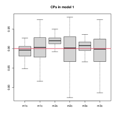
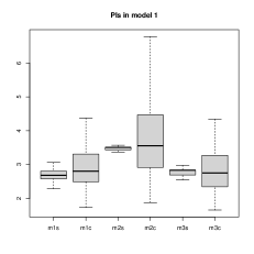
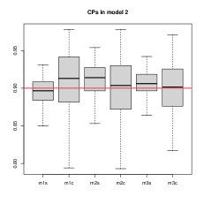
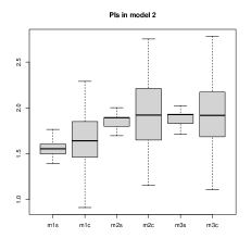
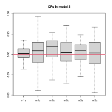
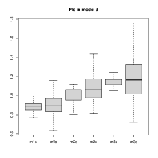
Figure A.1: Simulation A1: Misspecified regression model. Histogram of the 90% coverage probability (CP) and prediction interval length (PI) of the estimated prediction interval in the three models using the six methods. $n=100$.

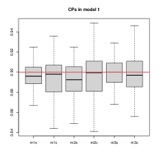
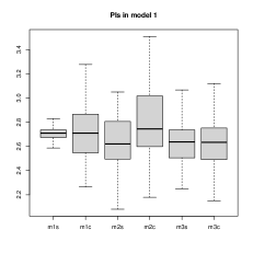
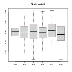
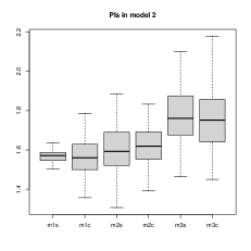
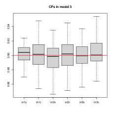
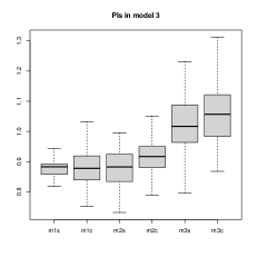
Figure A.2: Simulation A1: Misspecified regression model. Histogram of the 90% coverage probability (CP) and prediction interval length (PI) of the estimated prediction interval in the three models using the six methods. $n=500$.

Table A.2: Simulation A2: Misspecified measurement error model. The average and standard deviation of the coverage probabilities (CP (SD)), and the average and standard deviation of the lengths (LPI (SD)) of the estimated 90% prediction intervals.

	m1s	m1c	m2s	m2c	m3s	m3c
	$n=100$
	$m_{1}$
CP (SD)	0.878 (0.036)	0.905 (0.04)	0.919 (0.028)	0.903 (0.042)	0.908 (0.022)	0.897 (0.045)
LPI (SD)	2.558 (0.246)	3.417 (0.974)	3.798 (0.415)	4.204 (1.388)	2.815 (0.198)	2.877 (0.519)
	$m_{2}$
CP (SD)	0.883 (0.037)	0.901 (0.045)	0.919 (0.028)	0.903 (0.042)	0.908 (0.022)	0.897 (0.045)
LPI (SD)	2.676 (0.321)	2.885 (0.495)	3.798 (0.415)	4.204 (1.388)	2.815 (0.198)	2.877 (0.519)
	$m_{3}$
CP (SD)	0.884 (0.025)	0.891 (0.05)	0.906 (0.048)	0.906 (0.045)	0.899 (0.035)	0.896 (0.044)
LPI (SD)	0.901 (0.065)	0.931 (0.16)	1.055 (0.123)	1.136 (0.166)	1.218 (0.173)	1.254 (0.259)
	$n=500$
	$m_{1}$
CP (SD)	0.89 (0.02)	0.898 (0.022)	0.891 (0.026)	0.893 (0.025)	0.899 (0.017)	0. 9 (0.021)
LPI (SD)	2.616 (0.125)	2.74 (0.286)	2.697 (0.256)	2.861 (0.312)	2.675 (0.149)	2.688 (0.212)
	$m_{2}$
CP (SD)	0.885 (0.021)	0.898 (0.023)	0.891 (0.028)	0.898 (0.02)	0.903 (0.018)	0.899 (0.023)
LPI (SD)	1.546 (0.073)	1.617 (0.103)	1.63 (0.13)	1.72 (0.112)	1.948 (0.222)	1.944 (0.237)
	$m_{3}$
CP (SD)	0.896 (0.027)	0.898 (0.02)	0.887 (0.027)	0.898 (0.023)	0.895 (0.03)	0.899 (0.022)
LPI (SD)	0.94 (0.076)	0.905 (0.057)	0.911 (0.059)	0.961 (0.066)	1.153 (0.16)	1.184 (0.217)

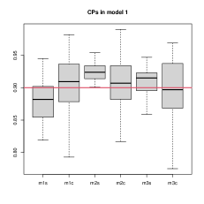
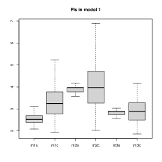
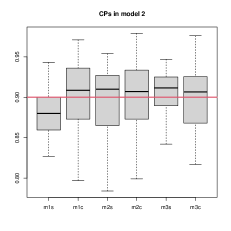
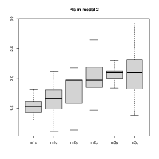
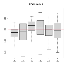
Figure A.3: Simulation A2: Misspecified measurement error model. Histogram of the 90% coverage probability (CP) and prediction interval length (PI) of the estimated prediction interval in the three models using the six methods when the distribution of $U$ is misspecified. $n=100$.

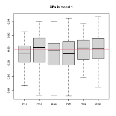
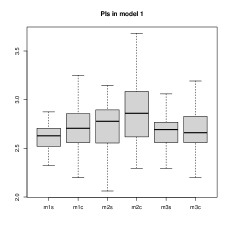
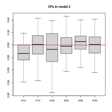
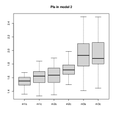
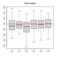
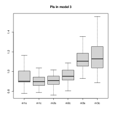
Figure A.4: Simulation A2: Misspecified measurement error model. Histogram of the 90% coverage probability (CP) and prediction interval length (PI) of the estimated prediction interval in the three models using the six methods when the distribution of $U$ is misspecified. $n=500$.

Table A.3: Simulation A3: Misspecified regression model and measurement error model. The average and standard deviation of the coverage probabilities (CP (SD)), and the average and standard deviation of the lengths (LPI (SD)) of the estimated 90% prediction intervals.

	m1s	m1c	m2s	m2c	m3s	m3c
	$n=100$
	$m_{1}$
CP (SD)	0.882 (0.021)	0.9 (0.041)	0.910 (0.030)	0.9 (0.04)	0.873 (0.025)	0.897 (0.042)
LPI (SD)	2.719 (0.207)	2.969 (0.484)	3.262 (0.326)	3.741 (1.15)	2.484 (0.201)	2.87 (0.507)
	$m_{2}$
CP (SD)	0.879 (0.021)	0.905 (0.04)	0.87 (0.031)	0.898 (0.038)	0.861 (0.03)	0.898 (0.042)
LPI (SD)	1.541 (0.085)	1.681 (0.187)	1.671 (0.154)	1.905 (0.313)	1.684 (0.209)	2.043 (0.378)
	$m_{3}$
CP (SD)	0.897 (0.024)	0.91 (0.035)	0.894 (0.047)	0.901 (0.041)	0.871 (0.03)	0.905 (0.04)
LPI (SD)	0.903 (0.054)	0.953 (0.114)	0.984 (0.127)	1.062 (0.151)	1.08 (0.177)	1.266 (0.234)
	$n=500$
	$m_{1}$
CP (SD)	0.886 (0.016)	0.897 (0.025)	0.880 (0.022)	0.899 (0.021)	0.892 (0.016)	0.898 (0.022)
LPI (SD)	2.739 (0.094)	2.86 (0.213)	2.551 (0.167)	2.802 (0.243)	2.6 (0.152)	2.673 (0.184)
	$m_{2}$
CP (SD)	0.884 (0.013)	0.901 (0.023)	0.875(0.022)	0.9 (0.019)	0.87 (0.019)	0.9 (0.022)
LPI (SD)	1.565 (0.035)	1.65 (0.1)	1.514 (0.092)	1.669 (0.095)	1.642 (0.174)	1.868 (0.192)
	$m_{3}$
CP (SD)	0.891 (0.017)	0.9 (0.021)	0.883 (0.022)	0.9 (0.022)	0.86 (0.028)	0.9 (0.022)
LPI (SD)	0.884 (0.03)	0.914 (0.056)	0.872 (0.048)	0.93 (0.059)	0.967 (0.104)	1.148 (0.179)

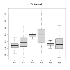
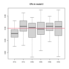
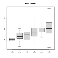
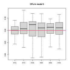
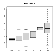
Figure A.5: Simulation A3: Misspecified regression model and measurement error model. Histogram of the 90% coverage probability (CP) and prediction interval length (PI) of the estimated prediction interval in the three models using the six methods when both the distributions of $U$ and $\epsilon$ are misspecified. $n=100$.

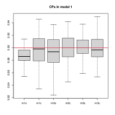
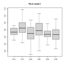
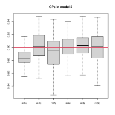
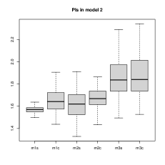
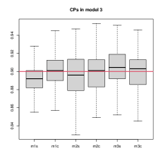
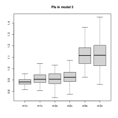
Figure A.6: Simulation A3: Misspecified regression model and measurement error model. Histogram of the 90% coverage probability (CP) and prediction interval length (PI) of the estimated prediction interval in the three models using the six methods when both the distributions of $U$ and $\epsilon$ are misspecified. $n=500$.

References

- (1)
- Buonaccorsi (1995) Buonaccorsi, J. (1995), ‘Prediction in the presence of measurement error: General discussion and an example predicting defoliation’, Biometrics 51, 1562–1569.
- Carroll et al. (2009) Carroll, R., Delaigle, A. & Hall, P. (2009), ‘Nonparametric prediction in measurement error models’, Journal of the American Statistical Association 104, 993–1003.
- Carroll et al. (2010) Carroll, R. J., Chen, X. & Hu, Y. (2010), ‘Identification and inference in nonlinear models using two samples with nonclassical measurement errors’, Journal of Nonparametric Statistics 22, 379–399.
- Carroll & Hall (1988) Carroll, R. J. & Hall, P. (1988), ‘Optimal rates of convergence for deconvolving a density’, Journal of the American Statistical Association 83, 1184–1186.
- Chen et al. (2008) Chen, X., Hu, Y. & Lewbel, A. (2008), ‘Nonparametric identification of regression models containing a misclassified dichotomous regressor without instruments’, Economics Letters 100, 381–384.
- Chen et al. (2009) Chen, X., Hu, Y. & Lewbel, A. (2009), ‘Nonparametric identification and estimation of nonclassical errors-in-variables models without additional information’, Statistica Sinica 19, 949–968.
- Datta et al. (2018) Datta, G., Delaigle, A., Hall, P. & Wang, L. (2018), ‘Semiparametric prediction intervals in small areas when auxiliary data are measured with error’, Statistica Sinica 28, 2309–2335.
- Fan (1991) Fan, J. (1991), ‘On the optimal rates of convergence for nonparametric deconvolution problems’, Annals of Statistics 19, 1257–1272.
- Ganse et al. (1983) Ganse, R., Amemiya, Y. & Fuller, W. A. (1983), ‘Prediction when both variables are subject to error, with application to earthquake magnitudes’, Journal of the American Statistical Association 78, 761–765.
- Hu & Sasaki (2017) Hu, Y. & Sasaki, Y. (2017), ‘Identification of paired nonseparable measurement error models’, Econometric Theory 33, 955–979.
- Hu & Schennach (2013) Hu, Y. & Schennach, S. (2013), ‘Nonparametric identification and semiparametric estimation of classical measurement error models without side information’, Journal of the American Statistical Association 108, 177–186.
- Hu & Schennach (2008) Hu, Y. & Schennach, S. M. (2008), ‘Instrumental variable treatment of nonclassical measurement error models’, Econometrica 76, 195–216.
- Hu et al. (2022) Hu, Y., Schennach, S. & Shiu, J.-L. (2022), ‘Identification of nonparametric monotonic regression models with continuous nonclassical measurement errors’, Journal of Econometrics 226, 269–294.
- Hu & Shiu (2018) Hu, Y. & Shiu, J.-L. (2018), ‘Nonparametric identification using instrumental variables: sufficient conditions for completeness’, Econometric Theory 34, 659–693.
- Hu et al. (2015) Hu, Y., Shiu, J.-L. & Woutersen, T. (2015), ‘Identification and estimation of single index models with measurement error and endogeneity’, Econometrics Journal 18, 347–362.
- Hu et al. (2016) Hu, Y., Shiu, J. & Woutersen, T. (2016), ‘Identification in nonseparable models with measurement error and endogeneity’, Economics Letters 144, 33–36.
- Jiang & Ma (2022) Jiang, F. & Ma, Y. (2022), ‘Poisson regression with error corrupted high dimensional features’, Statistica Sinica 32, 2023–2046.
- Jiang et al. (2024) Jiang, F., Ma, Y. & Carroll, R. J. (2024), ‘A spline-assisted semiparametric approach to nonparametric measurement error models’, Econometrics and Statistics .
- Jiang et al. (2023) Jiang, F., Zhou, Y., Liu, J. & Ma, Y. (2023), ‘On high dimensional poisson models with measurement error: hypothesis testing for nonlinear nonconvex optimization’, Annals of Statistics 51, 233–259.
- Kress (1999) Kress, R. (1999), Linear Integral Equtions, Springer-Verlag, New York.
- Landau et al. (2021) Landau, S., Murphy, A. E., Lee, J. Q., Ward, T. J. & Jagust, W. (2021), ‘Florbetapir (av45) processing methods’.
- Lei et al. (2018) Lei, J., G’Sell, M., Rinaldo, A., Tibshirani, R. J. & Wasserman, L. (2018), ‘Distribution-free predictive inference for regression’, Journal of the American Statistical Association 113, 1094–1111.
- Leuzy et al. (2016) Leuzy, A., Chiotis, K., Hasselbalch, S. G., Rinne, J. O., de Mendoncca, A., Otto, M., Lleo, A., Castelo-Branco, M., Santana, I., Johansson, J. et al. (2016), ‘Pittsburgh compound b imaging and cerebrospinal fluid amyloid- in a multicentre european memory clinic study’, Brain 139(9), 2540–2553.
- Li & Ma (2024) Li, M. & Ma, Y. (2024), ‘An update on measurement error modeling’, Annual Review of Statistics and Its Application .
- Masters & Bateman (2015) Masters, C. & Bateman, R. (2015), ‘blennow k, rowe cc, sperling ra, cummings jl. alzheimer’s disease’, Nature Reviews Disease Primers 15059.
- Mattsson et al. (2017) Mattsson, N., Lönneborg, A., Boccardi, M., Blennow, K., Hansson, O., for the Roadmap, G. T. F. et al. (2017), ‘Clinical validity of cerebrospinal fluid a42, tau, and phospho-tau as biomarkers for alzheimer’s disease in the context of a structured 5-phase development framework’, Neurobiology of aging 52, 196–213.
- Palmqvist et al. (2015) Palmqvist, S., Zetterberg, H., Mattsson, N., Johansson, P., Minthon, L., Blennow, K., Olsson, M., Hansson, O., Initiative, A. D. N., Group, S. B. S. et al. (2015), ‘Detailed comparison of amyloid pet and csf biomarkers for identifying early alzheimer disease’, Neurology 85(14), 1240–1249.
- Romano et al. (2019) Romano, Y., Patterson, E. & Candes, E. (2019), ‘Conformalized quantile regression’, Advances in neural information processing systems 32.
- Scheltens et al. (2016) Scheltens, P., Blennow, K., Breteler, M. M., De Strooper, B., Frisoni, G. B., Salloway, S. & Van der Flier, W. M. (2016), ‘Alzheimer’s disease.’, Lancet (London, England) 388(10043), 505–517.
- Schipke et al. (2017) Schipke, C. G., Koglin, N., Bullich, S., Joachim, L. K., Haas, B., Seibyl, J., Barthel, H., Sabri, O. & Peters, O. (2017), ‘Correlation of florbetaben pet imaging and the amyloid peptide aß42 in cerebrospinal fluid’, Psychiatry Research: Neuroimaging 265, 98–101.
- Shaw et al. (2016) Shaw, L. M., Figurski, M., Waligorska, T. & Trojanowski, J. Q. (2016), ‘An overview of the first 8 adni csf batch analyses’.
- Tsiatis & Ma (2004) Tsiatis, A. A. & Ma, Y. (2004), ‘Locally efficient semiparametric estimators for functional measurement error models’, Biometrika 91, 835–848.
- Vershynin (2010) Vershynin, R. (2010), ‘Introduction to the non-asymptotic analysis of random matrices’, arXiv preprint arXiv:1011.3027 .
- Zhang et al. (2019) Zhang, X., Ma, Y. & Carroll, R. J. (2019), ‘Malmem: Model averaging in linear measurement error models’, Journal of the Royal Statistical Society, Series B. 81.
- Zhang et al. (2021) Zhang, X., Zhang, X. & Ma, Y. (2021), ‘A model averaging treatment to multiple instruments in poisson model with errors’, Canadian Journal of Statistics .