Power-law relaxation of a confined diffusing particle subject to resetting with memory

Abstract

We study the relaxation of a Brownian particle with long range memory under confinement in one dimension. The particle diffuses in an arbitrary confining potential and resets at random times to previously visited positions, chosen with a probability proportional to the local time spent there by the particle since the initial time. This model mimics an animal which moves erratically in its home range and returns preferentially to familiar places from time to time, as observed in nature. The steady state density of the position is given by the equilibrium Boltzmann-Gibbs distribution, as in standard diffusion, while the transient part of the density can be obtained through a mapping of the Fokker-Planck equation of the process to a Schrödinger eigenvalue problem. Due to memory, the approach at large time toward the steady state is critically self-organised, in the sense that it always follows a sluggish power-law form, in contrast to the exponential decay that characterises Markov processes. The exponent of this power-law depends in a simple way on the resetting rate and on the leading relaxation rate of the Brownian particle in the absence of resetting. We apply these findings to several exactly solvable examples, such as the harmonic, V-shaped and box potentials.

1 Introduction

Let us consider a single Brownian particle which, in addition to diffusion, undergoes a resetting process with rate $r$ to previously visited positions. Resetting follows a stochastic rule that incorporates memory effects: the particle that resets at some time $t$ chooses uniformly at random a preceding time $0\leq t^{\prime}\leq t$, i.e., with probability density $1/t$, and occupies the position at which it was located at $t^{\prime}$ again. Thus the resetting move tends to bring the particle near the most visited positions in the past. This model was introduced in the context of random walks on lattices and solved exactly in Ref. [1]. The model was further extended to a free Brownian particle on the line [2]. The position distribution at time $t$ was found to approach a Gaussian form at late times with the variance growing anomalously slowly as $(2D/r)\,\ln t$ for large $t$, where $D$ is the diffusion constant of the particle. This slow dynamics emerges from the resetting induced memory effect: the particle is sluggish to move away from its familiar territory, where the most visited sites are located. Nevertheless, the position distribution is always time-dependent and does not approach a stationary state at late times, contrary to diffusive processes subject to resetting to a single point, which generically admit non-equilibrium steady states (NESSs) [3, 4, 5].

Various other generalisations of this simple model have been studied in the recent past, for instance by considering a decaying memory [6], Lévy flights [7] or active particles [8]. A central limit theorem and an anomalous large deviation principle have also been established for a class of memory walks of this type, for a broad range of memory kernels [9, 10]. The rigorous proofs of these latter results are based on a connection between the resetting process to previous sites and the growth of weighted random recursive trees.

In a more applied context, random walks with long range memory have become increasingly useful in ecology for the description and analysis of animal mobility. There is mounting evidence that animals do not follow purely Markov processes but also use their memory and tend to revisit preferred places during ranging [11, 12, 13, 14, 15, 16]. The model above was able to describe quantitatively the movement patterns of Capuchin monkeys in the wild [1], as well as of individual elks released in an unknown environment [17]. Another feature shared by many animal trajectories is spatial localisation, by opposition to unbounded diffusion, as home ranges are often clearly identifiable. The range-resident behaviour of animals can be modelled by incorporating in the simple random walk a central place (such as a den) toward which the walker is attracted, producing an effective $|x|$ potential and therefore a stationary ’equilibrium’ state at large times [18]. Recent studies have considered harmonic potentials and Ornstein–Uhlenbeck (OU) processes as the starting point of models of home range movements of increasing complexity [19, 20, 21].

In this paper, we study a Brownian particle in one dimension under the combined effects of confinement by an external potential $U(x)$ and of memory, as described in the rule above. In this situation, we expect the position distribution $P_{r}(x,t)$ to approach a stationary form at late times, where the subscript $r$ in $P_{r}(x,t)$ denotes the nonzero resetting rate. We first recall that in the absence of resetting, i.e., for $r=0$, the system approaches the equilibrium stationary state characterised by the Gibbs-Boltzmann distribution

$$P_{0}^{\rm st}(x)=\frac{1}{Z}\,e^{-\frac{1}{D}\,U(x)}\,,$$ (1)

where the friction coefficient of the particle is set to $1$ from now on and the partition function $Z=\int_{-\infty}^{\infty}e^{-U(x)/D}\,dx$ normalises the distribution to unity. We assume that $U(x)$ is sufficiently confining so that the integral $Z$ is finite. Moreover, the position distribution relaxes generically to the equilibrium measure in Eq. (1) exponentially fast. More precisely, writing $P_{0}(x,t)=P_{0}^{\rm st}(x)+P_{0}^{\rm tr}(x,t)$ where the superscript ’${\rm tr}$’ denotes the time-dependent transient part of the distribution, one finds that for large $t$

$$P_{0}^{\rm tr}(x,t)=P_{0}(x,t)-P_{0}^{\rm st}(x)\sim e^{-\lambda_{1}t}\,,$$ (2)

where $\lambda_{1}$ denotes the first nonzero eigenvalue of the diffusion operator in the confining potential $U(x)$. The precise value of $\lambda_{1}$ depends on the potential $U(x)$. The $x$ dependence of the leading transient is implicit in the amplitude on the right hand side (rhs) of Eq. (2). In fact, the decay exponent $\lambda_{1}$, up to a multiplicative constant, is precisely the gap between the first excited state $E_{1}$ and the ground state $E_{0}=0$ of the associated Schrödinger operator [22] (see Section II for details).

Here, we investigate the behaviour of the position distribution $P_{r}(x,t)$, when one switches memory on with a non-zero rate $r$. In the presence of a finite resetting rate $r>0$, we again expect the position distribution to approach a stationary form $P_{r}^{\rm st}(x)=P_{r}(x,t\to\infty)$ at late times. Our first goal is to characterise this stationary position distribution. Moreover, it is also important to study how the system relaxes to this stationary state at late times for nonzero $r$, i.e., how the result in Eq. (2) gets modified with a nonzero $r$. Our main results are twofold:

• $(i)$ We show that the stationary position distribution $P_{r}^{\rm st}(x)$ for nonzero $r$ remains of the Gibbs-Boltzmann form independently of $r$, i.e.,

  $$P_{r}^{\rm st}(x)=\frac{1}{Z}\,e^{-\frac{1}{D}\,U(x)}\,.$$ (3)

  Like in the $r=0$ case, this stationary state for $r>0$ is actually an equilibrium state. This property markedly differs from the well-studied problem of a Brownian particle in a potential $U(x)$ and subject to resetting to a fixed point [23, 24, 25, 26, 27, 28, 29, 30, 31], a case that manifestly violates detailed balance and generates a NESS.

• $(ii)$ Even more interestingly, we find that in complete contrast to the exponential decay in Eq. (2) for $r=0$, the relaxation to the stationary state for $r>0$ is always algebraic, or “critical”. More precisely, the analogue of Eq. (2) now reads for large $t$

  $$P_{r}^{\rm tr}(x,t)=P_{r}(x,t)-P_{r}^{\rm st}(x)\sim t^{-\theta_{1}}$$ (4)

  where the dependence of the amplitude on $x$ and $r$ is implicit. The exponent $\theta_{1}$ depends on $r$ and also on the confining potential $U(x)$. In fact we show that the exponent $\theta_{1}$ can be expressed in terms of the decay rate $\lambda_{1}$ of the resetting-free case via the exact relation

  $$\theta_{1}=\frac{\lambda_{1}}{r+\lambda_{1}}\,.$$ (5)

  Thus as $r$ increases, the exponent $\theta_{1}$ decreases and the relaxation dynamics becomes slower.

The rest of the paper is organised as follows. In Section 2, to set the stage and our notations, we recall well-known results and the method to study diffusion in a confining potential in the absence of resetting, i.e., for $r=0$. In Section 3, we derive our main results for the stationary state and the transient part in the presence of a finite resetting rate $r>0$. In Section 4, we exemplify the calculations for the harmonic and $|x|$ potentials. Section 5 is devoted to the case of a particle in a box, $x\in[0,L]$ with reflecting boundary conditions at the two boundaries, where we derive the full probability distribution $P_{r}(x,t)$ at all times. A comparison of the theoretical results with numerical simulations is given in Section 6 and we conclude in Section 7.

2 Diffusion in a confining potential without resetting

In this section, we recall the basic results and the general method to compute the time-dependent position distribution of an over-damped Brownian particle diffusing in the presence of a confining potential $U(x)$ [22]. The position $x(t)$ of the particle evolves via the over-damped Langevin equation

$$\frac{dx}{dt}=-U^{\prime}(x)+\eta(t)\,,$$ (6)

where $\eta(t)$ is a Gaussian white noise with zero mean $\langle\eta(t)\rangle=0$ and a delta correlator: $\langle\eta(t)\eta(t^{\prime})\rangle=2\,D\,\delta(t-t^{\prime})$, with $D$ the diffusion constant. (We recall that the friction coefficient is set to unity.) The associated Fokker-Planck equation reads

$$\partial_{t}P_{0}(x,t)=D\,\partial_{x}^{2}P_{0}(x,t)+\partial_{x}\left[U^{\prime}(x)\,P_{0}(x,t)\right]\,,$$ (7)

starting from the initial condition $P_{0}(x,0)=\delta(x-x_{0})$ and satisfying the boundary conditions: $P_{0}(x\to\pm\infty,t)=0$.

To solve this partial differential equation, one can use the method of separation of variables and use the ansatz

$$P_{0}(x,t)=\phi(x)\,f(t)\,.$$ (8)

Substituting (8) in (7) and dividing both sides by $\phi(x)\,f(t)$ one gets

$$\frac{{\dot{f}}(t)}{f(t)}=\frac{D\phi^{\prime\prime}(x)+U^{\prime}(x)\,\phi^{\prime}(x)+U^{\prime\prime}(x)\,\phi(x)}{\phi(x)}=-\lambda\,,$$ (9)

where $\lambda$ is a constant independent of $x$ and $t$. Solving for $f(t)$ gives $f(t)=A_{0}\,e^{-\lambda t}$ where $A_{0}$ is a constant and one must have $\lambda\geq 0$ so that the solution does not diverge as $t\to\infty$. The function $\phi(x)$ satisfies a second order differential equation

$$D\,\phi^{\prime\prime}(x)+U^{\prime}(x)\,\phi^{\prime}(x)+U^{\prime\prime}(x)\,\phi(x)=-\lambda\,\phi(x)\,,$$ (10)

where $\lambda$ plays the role of an eigenvalue, yet to be determined. One can further reduce this eigenvalue equation to a more familiar Schrödinger form via the substitution

$$\phi(x)=e^{-\frac{1}{2D}\,U(x)}\,\psi(x)\,.$$ (11)

It is then easy to see that $\psi(x)$ satisfies the time-independent Schrödinger equation (setting $m=\hbar=1$)

$$-\frac{1}{2}\,\psi^{\prime\prime}(x)+V_{Q}(x)\,\psi(x)=\frac{\lambda}{2D}\,\psi(x)\,,$$ (12)

where the quantum potential $V_{Q}(x)$ is expressed in terms of the classical potential $U(x)$ via the relation

$$V_{Q}(x)=-\frac{1}{4D}U^{\prime\prime}(x)+\frac{1}{8D^{2}}\,[U^{\prime}(x)]^{2}\,.$$ (13)

Thus one needs to solve the Schrödinger equation (12), find its spectrum, i.e., the eigenvalues $E_{n}=\lambda_{n}/(2D)$ and the associated eigenfunctions $\psi_{\lambda_{n}}(x)$. Note that in general, the spectrum of $V_{Q}(x)$ may consist of both bound and scattering states, even though $U(x)$ may be fully confining. Once we have the full spectrum, one can then write down the most general solution of Eq. (7) as a linear combination of these eigenfunctions

$$P_{0}(x,t)=\sum_{n}a_{\lambda_{n}}\,\left[e^{-\frac{1}{2D}\,U(x)}\,\psi_{\lambda_{n}}(x)\right]\,e^{-\lambda_{n}t}\,,$$ (14)

where the coefficients $\{a_{\lambda_{n}}\}$ can be determined from the initial condition. Note that the quantum potential $V_{Q}(x)$ is such that its ground state corresponds to zero energy $\lambda_{0}/2D=E_{0}=0$, with eigenfunction $\psi_{0}(x)\propto e^{-U(x)/{2D}}$ as one can easily check. Thus separating the ground state from the rest of the spectrum in Eq. (14), we get

$$P_{0}(x,t)=a_{0}\,e^{-\frac{1}{D}\,U(x)}+\sum_{\lambda_{n}>0}a_{\lambda_{n}}\,\left[e^{-\frac{1}{2D}\,U(x)}\,\psi_{\lambda_{n}}(x)\right]\,e^{-\lambda_{n}\,t}\,.$$ (15)

One then immediately identify the first term on the rhs of (15) as the stationary Gibbs distribution

$$P_{0}^{\rm st}(x)=a_{0}e^{-\frac{1}{D}\,U(x)}\;\quad{\rm with}\quad a_{0}=\frac{1}{Z}=\frac{1}{\int_{-\infty}^{\infty}e^{-U(x)/D}\,dx}\,.$$ (16)

The second term in (15), summing over all nonzero modes, represents the transient part of the distribution $P_{0}^{\rm tr}(x,t)$. If the first excited state $\lambda_{1}>0$ is strictly positive, i.e., well separated from the ground state $\lambda_{0}=0$, then it governs the leading late time decay of the transient and one obtains

$$P_{0}^{\rm tr}(x,t)\approx a_{\lambda_{1}}\,e^{-\frac{1}{2D}\,U(x)}\,\psi_{\lambda_{1}}(x)\,e^{-\lambda_{1}\,t}\,.$$ (17)

Note that the result in Eq. (17) holds provided that $a_{\lambda_{1}}\neq 0$. Sometimes, the initial condition may have a special symmetry that renders $a_{\lambda_{1}}=0$. In that case, the leading decay will be governed by the next nonzero excited state.

Let us remark that the result in Eq. (17) is valid for any confining potential $U(x)$, such that $(i)$ the integral $Z=\int_{-\infty}^{\infty}e^{-U(x)/D}\,dx$ exists, $(ii)$ the associated quantum potential $V_{Q}(x)$ in Eq. (13) is such that its first excited state has eigenvalue $\lambda_{1}>0$ (recall that the ground state has zero energy if a steady state exists). In addition, the leading decay in Eq. (17) will be a pure exponential if $\lambda_{1}<\lambda_{2}$, i.e., there is a nonzero gap between the first and the second excited state. There are some potentials $U(x)$ for which $\lambda_{1}>0$ may be gapped from the ground state, but then there is a continuum of scattering states beyond $\lambda_{1}$. In this case, depending on how the density of scattering states vanishes as one approaches $\lambda_{1}$ from above, one may have an additional sub-leading algebraic correction to the leading exponential decay $\sim e^{-\lambda_{1}\,t}$. We discuss below two examples that can be explicitly solved to illustrate these features.

Ornstein-Uhlenbeck (OU) process. As a first simple example, consider the OU process of stiffness $\mu>0$, for which $U(x)=\mu x^{2}/2$. In this case, the quantum potential in Eq. (13) reads

$$V_{Q}(x)=\frac{\mu^{2}}{8D^{2}}\,x^{2}-\frac{\mu}{4D}\,.$$ (18)

Thus, one has a quantum harmonic oscillator of mass $m=1$ and frequency $\omega=\mu/(2D)$, with the height of the potential shifted by $\mu/(4D)$. Consequently, the energy levels are well separated from each other and are given by

$$E_{n}=\left(n+\frac{1}{2}\right)\,\omega-\frac{\mu}{4D}=n\,\frac{\mu}{2D}\,,\quad{\rm with}\quad n=0,1,2\ldots$$ (19)

The eigenvalues are given by $\lambda_{n}=2DE_{n}=n\,\mu$ and the leading transient in Eq. (17) decays as

$$P_{0}^{\rm tr}(x,t)\approx a_{\lambda_{1}}\,e^{-\frac{\mu}{2D}\,x^{2}}\,\psi_{\lambda_{1}}(x)\,e^{-\mu\,t}\,,$$ (20)

where $\psi_{1}(x)$ represents the eigenfunction associated with the first excited state of the harmonic oscillator. Note that if the initial condition is symmetric, e.g., when $P_{0}(x)=\delta(x)$, this symmetry is preserved at all times, indicating that only the even eigenfunctions contribute to the spectral decomposition in Eq. (14). This means that all the odd coefficients vanish: $a_{\lambda_{2m+1}}=0$ for all $m=0,1,2,\ldots$. In that case, the leading transient corresponds to the second excited state of the harmonic oscillator and $P_{0}^{\rm tr}(x,t)$ decays as $\sim e^{-2\mu t}$ at late times.

The potential $U(x)=F\,|x|$ with $F>0$. This is an interesting example since, in this case, the quantum potential in Eq. (13) reads

$$V_{Q}(x)=-\frac{F}{2D}\,\delta(x)+\frac{F^{2}}{8D^{2}}\,.$$ (21)

This quantum potential has a single bound state at $E=0$ and a continuum of excited states with energies $E\geq E_{1}=F^{2}/(8D^{2})$. Thus there is a gap $\lambda_{1}=2D\,E_{1}=F^{2}/(4D)$, and we expect that the transient in Eq. (17) will decay, to leading order for large $t$, exponentially as $e^{-\lambda_{1}t}\sim e^{-F^{2}t/(4D)}$. However, unlike in the harmonic oscillator example above, the eigenvalue $\lambda_{1}$ is not isolated here and there is a continuum of scattering states above $E_{1}$. Moreover, the density of such states vanishes as $\sqrt{E-E_{1}}$ as $E\to E_{1}$ from above (see Section 4 further) and the leading decay of the transient in Eq. (17) now behaves as $e^{-F^{2}t/(4D)}\,t^{-3/2}$. The sub-leading $t^{-3/2}$ decay emerges from replacing the sum in Eq. (15) by an integral above $E_{1}$. Since the density of states vanishes as $\sqrt{E-E_{1}}$, this leads to the power law correction $t^{-3/2}$ multiplying the leading exponential $e^{-F^{2}t/(4D)}$ [32].

3 Diffusion in a confining potential in the presence of resetting

We now allow the particle to perform resetting moves, in addition to the diffusion in the confining external potential. Let us recall the memory-driven resetting dynamics. At time $t$, with rate $r$ the particle chooses any previous time in the past $0\leq t^{\prime}<t$ with uniform probability density $1/t$ and resets to the position that it occupied at that previous instant $t^{\prime}$. Let $P_{r}(x,t)$ denote the position distribution at time $t$. To take into account the memory effect, we now need to define the two-point function $P_{r}(x,t\,;x^{\prime},t^{\prime})$, which is the joint probability density for the particle to be near $x^{\prime}$ at $t^{\prime}$ and near $x$ at $t$, with $t^{\prime}\leq t$. Clearly, if we integrate over one of the one of the positions, we recover the marginal one-point probability density

$$\int_{-\infty}^{\infty}P_{r}(x,t\,;x^{\prime},t^{\prime})\,dx^{\prime}=P_{r}(x,t)\quad{\rm and}\quad\int_{-\infty}^{\infty}P_{r}(x,t\,;x^{\prime},t^{\prime})\,dx=P_{r}(x^{\prime},t^{\prime}).$$ (22)

With these ingredients at hand, we can now write down the Fokker-Planck equation for the evolution of the one-point position distribution $P_{r}(x,t)$ as

$$\partial_{t}P_{r}(x,t) = D\,\partial_{x}^{2}P_{r}(x,t)+\partial_{x}\left(U^{\prime}(x)\,P_{r}(x,t)\right)-r\,P_{r}(x,t)$$ (23)

$$+\frac{r}{t}\,\int_{0}^{t}dt^{\prime}\int_{-\infty}^{\infty}dx^{\prime}\,P_{r}(x^{\prime},t;x,t^{\prime})\,.$$

The first two terms on the rhs describe, as before, the diffusion in the external potential $U(x)$. The third term describes the loss of probability density from position $x$ at time $t$ due to resetting to other positions. The last term on the rhs describes the gain in the probability density at $x$ at time $t$ due to resetting from other positions labelled by $x^{\prime}$. If the particle has to reset to $x$ from $x^{\prime}$ at time $t$, it must have been at $x$ at a previous time $t^{\prime}\leq t$ and the probability density of this event is simply the two-point function $P_{r}(x^{\prime},t;x,t^{\prime})$. Finally, we need to integrate over all positions $x^{\prime}$ from which the particle may arrive at $x$ by resetting. The reason for the solvability for the one-point position distribution in this model can then traced back to the second relation in Eq. (22), which allows us to write a closed equation for the one-point function (without involving multiple-point functions) provided that the resetting rate $r$ is independent of the position. We obtain

$$\partial_{t}P_{r}(x,t)=D\,\partial_{x}^{2}P_{r}(x,t)+\partial_{x}\left(U^{\prime}(x)\,P_{r}(x,t)\right)-r\,P_{r}(x,t)+\frac{r}{t}\,\int_{0}^{t}dt^{\prime}\,P_{r}(x,t^{\prime})\,.$$ (24)

It is easy to check that the total probability $\int_{-\infty}^{\infty}P_{r}(x,t)\,dx$ remains conserved and equals unity due to the initial condition, e.g., $P_{r}(x,0)=\delta(x-x_{0})$. One also needs to impose the vanishing boundary conditions as $x\to\pm\infty$, i.e., $P_{r}(x\to\pm\infty,t)=0$ for all $t$. Evidently, for $r=0$, Eq. (24) reduces to the standard Fokker-Planck equation (7).

To solve the Fokker-Planck equation (24), we follow the same route as in the $r=0$ case, namely, we use the method of separation of variables with the ansatz

$$P_{r}(x,t)=\phi(x)\,f_{r}(t)\,.$$ (25)

Substituting (25) in Eq. (24), dividing both sides by $\phi(x)f_{r}(t)$ and assembling the only-time dependent and only-space dependent parts separately gives

$$\frac{{\dot{f}_{r}}(t)}{f_{r}(t)}+r-\frac{r}{t\,f_{r}(t)}\,\int_{0}^{t}f_{r}(t^{\prime})\,dt^{\prime}=\frac{D\phi^{\prime\prime}(x)+U^{\prime}(x)\,\phi^{\prime}(x)+U^{\prime\prime}(x)\,\phi(x)}{\phi(x)}=-\lambda\,,$$ (26)

where $\lambda\geq 0$ is a constant independent of $x$ and $t$. Note that the space-dependent function $\phi(x)$ is independent of $r$ and satisfies the same eigenvalue equation (10) as the $r=0$ case. Consequently, the analysis of the spatial part is exactly as in the $r=0$ case discussed in the previous section. In particular, we get

$$\phi(x)=e^{-\frac{1}{2D}\,U(x)}\,\psi(x)\,,$$ (27)

where $\psi(x)$ satisfies the Schrödinger equation (10), with the same eigenvalues $\lambda_{n}$’s as in the $r=0$ case.

Thus, the $r$-dependence enters only in the time-dependent part $f_{r}(t)$ of the solution. For a given $\lambda$, we get from Eq. (26) a second order ordinary differential equation for $f_{r}(t)$

$${\dot{f}_{r}}(t)+(r+\lambda)\,f_{r}(t)-\frac{r}{t}\,\int_{0}^{t}f_{r}(t^{\prime})\,dt^{\prime}=0\,.$$ (28)

Multiplying this equation by $t$ and taking the time derivative, one obtains

$$t{\ddot{f}_{r}}(t)+[1+(r+\lambda)t]\,\dot{f_{r}}(t)+\lambda f_{r}(t)=0\,.$$ (29)

Through the change of variable $z=-(\lambda+r)t$ with $g(z)\equiv f(t)$, Eq. (29) can be recast as a confluent hypergeometric equation,

$$z\frac{d^{2}g(z)}{dz^{2}}+(b-z)\frac{dg(z)}{dz}-ag(z)=0,$$ (30)

with $b=1$ and $a=\lambda/(\lambda+r)$. The differential equation (30) has two linearly independent solutions denoted by $M(a,b,z)$ and $U(a,b,z)$ [33]. Hence, the most general solution of Eq. (29) can be expressed as

$$f_{r}(t)=c_{1}\,M\left(\frac{\lambda}{r+\lambda},1,-(r+\lambda)t\right)+c_{2}\,\,U\left(\frac{\lambda}{r+\lambda},1,-(r+\lambda)t\right)\,,$$ (31)

where $c_{1}$ and $c_{2}$ are two arbitrary constants. The solution must be finite at all $t$, in particular at $t=0$. The small argument asymptotics of the two solutions are given by [33]

$$M(a,b,z) \to 1\,\quad\quad\quad{\rm as}\quad z\to 0$$ (32)

$$U(a,b,z) \to \frac{1}{\Gamma(a)\,z}\,\quad{\rm as}\quad z\to 0\,.$$ (33)

Consequently, the divergence as $t\to 0$ in Eq. (31) is avoided by setting $c_{2}=0$, and our solution simply reads

$$f_{r}(t)=M\left(\frac{\lambda}{r+\lambda},1,-(r+\lambda)t\right)\,.$$ (34)

where we have set $c_{1}=1$ by absorbing this constant into the amplitude of the eigenmode. Importantly, using the identity $M(0,b,z)=1$, we recover $f_{r}(t)=1$ for $\lambda=0$. This means that the solution $\phi(x)$ with $\lambda=0$ in the eigenvalue equation (26), given by the Boltzmann-Gibbs distribution $\phi(x)=a_{0}e^{-\frac{1}{D}U(x)}$, is also a stationary state when $r>0$.

To obtain the asymptotic behaviour of $f_{r}(t)$ in time for $\lambda>0$, it is useful to recall here some basic properties of the confluent hypergeometric function $M(a,b,z)\equiv{{}_{1}}F_{1}(a,b,z)$. It has a simple power series expansion

$$M(a,b,z)=1+\frac{a}{b}\,z+\frac{a(a+1)}{b(b+1)}\,\frac{z^{2}}{2!}+\frac{a(a+1)(a+2)}{b(b+1)(b+2)}\,\frac{z^{3}}{3!}+\ldots\,,$$ (35)

whereas for large negative arguments, we have [33]

$$M(a,b,-z)\simeq\frac{\Gamma(b)}{\Gamma(b-a)}\,z^{-a}\,\quad{\rm as}\quad z\to\infty\,.$$ (36)

Consequently, $f_{r}(t)$ in Eq. (34) behaves for large $t$ as a power-law,

$$f_{r}(t)\simeq\frac{(r+\lambda)^{-\frac{\lambda}{r+\lambda}}}{\Gamma\left(\frac{r}{r+\lambda}\right)}\,t^{-\frac{\lambda}{r+\lambda}}\,.$$ (37)

Note that this result does not hold for $r=0$, as the prefactor in Eq. (37) vanishes in this case. Rather, the exponential decay $f_{r}(t)=e^{-\lambda t}$ is recovered by setting $r=0$ directly in Eq. (34), since $M(1,1,-z)=e^{-z}$.

Finally, combining the time-dependent part $f_{r}(t)$ and the space-dependent part that involves the set of all eigenvalues of the Schrödinger operator, we can express the full solution of $P_{r}(x,t)$ as the following exact spectral decomposition

$$P_{r}(x,t)=e^{-\frac{1}{2D}\,U(x)}\sum_{n}a_{\lambda_{n}}\,\psi_{\lambda_{n}}(x)\,M\left(\frac{\lambda_{n}}{r+\lambda_{n}},1,-(r+\lambda_{n})t\right)\,.$$ (38)

As in the $r=0$ case before, we will now separate out the stationary mode corresponding to the ground state $n=0$ with $\lambda_{0}=0$ from the transient part and rewrite Eq. (38) as

$$P_{r}(x,t)=a_{0}\,e^{-\frac{1}{D}\,U(x)}+e^{-\frac{1}{2D}\,U(x)}\sum_{n>0}a_{\lambda_{n}}\,\psi_{\lambda_{n}}(x)\,M\left(\frac{\lambda_{n}}{r+\lambda_{n}},1,-(r+\lambda_{n})t\right).$$ (39)

At late times, using the asymptotic behaviour of $f_{r}(t)$ in Eq. (37), it follows that the $n$-th mode in the second term on the rhs decays at late times as a power law $\sim t^{-\frac{\lambda_{n}}{r+\lambda_{n}}}$ for $\lambda_{n}>0$. Consequently, the sum in Eq. (39) represents the transient part $P_{r}^{\rm tr}(x,t)$, while the first term that is independent of $t$ represents the stationary solution.

Hence, we come to the two main results announced in the Introduction. First, the stationary solution

$$P_{r}^{\rm st}(x)=a_{0}e^{-\frac{1}{D}\,U(x)}\;\quad{\rm with}\quad a_{0}=\frac{1}{Z}=\frac{1}{\int_{-\infty}^{\infty}e^{-U(x)/D}\,dx}\,,$$ (40)

is independent of $r$ and remains with the Gibbs-Boltzmann form as in the $r=0$ case. This solution corresponds to an equilibrium state, since local detailed balance is fulfilled even with $r>0$. This can be understood by considering two small disjoint regions $[x,x+\delta_{x}]$ and $[y,y+\delta_{y}]$, which have been occupied until time $t$ for an total amount of time $\tau_{x}(t)$ and $\tau_{y}(t)$, respectively. The probability that the particle takes a move from the region $x$ to $y$ by resetting at time $t$ is $\delta_{x}P^{\rm st}(x)w^{(r)}_{x\to y}$, where the transition rate is given by $w^{(r)}_{x\to y}=r\tau_{y}(t)/t$ due to the preferential revisit rule. Since $\delta_{x}P^{\rm st}(x)\simeq\tau_{x}(t)/t$ at large $t$, the above transition probability reads $r\tau_{y}(t)\tau_{x}(t)/t^{2}$, which is symmetric with respect to $x$ and $y$, implying detailed balance. This property is a specificity of the linear reinforcement rule.

Secondly, the leading behaviour of the transient part decays as

$$P_{r}^{\rm tr}(x,t)\sim e^{-\frac{1}{2D}\,U(x)}\,\psi_{\lambda_{1}}(x)\,t^{-\theta_{1}}\,,\quad{\rm with}\quad\theta_{1}=\frac{\lambda_{1}}{r+\lambda_{1}}\,,$$ (41)

where $\lambda_{1}=\min_{n\in{\mathbb{N}}^{+}}\{\lambda_{n}\}$ represents the gap between the ground state and the first excited state of the underlying Schrödinger operator of the $r=0$ case. Thus, unlike the stationary solution that remains unaffected by resetting, the transient part gets modified drastically if $r>0$. It now decays very slowly as a power law at late times with a non-universal exponent $\theta_{1}=\lambda_{1}/(r+\lambda_{1})$ comprised in the interval $[0,1]$ and that decreases with increasing $r$, indicating that the dynamics get slower and slower due to resetting. This result is completely general, valid for any shape of the confining potential.

4 Examples of confining potentials

4.1 Harmonic potential

A specific example corresponds to the OU process where $U(x)=\mu x^{2}/2$. In this case, the quantum potential $V_{Q}(x)$ represents a harmonic oscillator with energy eigenvalues $E_{n}=n\,\frac{\mu}{2D}$ or $\lambda_{n}=n\,\mu$ with $n=0,1,2\ldots$, see Eqs. (18)-(19). Consequently, $\lambda_{1}=\mu$ and the exponent $\theta_{1}$ in Eq. (41) is given by

$$\theta_{1}=\frac{\mu}{r+\mu}\,.$$ (42)

4.2 V-shaped potential

For the case $U(x)=F\,|x|$, it turns out that the transient part of the density behaves as

$$P_{r}^{\rm tr}(x,t)\sim(\ln t)^{-3/2}\,t^{-\theta_{1}}\,,\quad{\rm with}\quad\theta_{1}=\frac{\lambda_{1}}{r+\lambda_{1}}=\frac{F^{2}}{4Dr+F^{2}}\,.$$ (43)

As discussed in Section 2, the first excited state $\lambda_{1}=F^{2}/(4D)$ is well separated from the ground state $E_{0}=0$, but there is a continuum of excited states above $E_{1}=\lambda_{1}/(2D)$ whose density vanishes as $\sqrt{E-E_{1}}$ as $E\to E_{1}$, as shown below. This leads to additional logarithmic corrections to the leading power law decay in Eq. (41).

Let us now derive this result. We recall that the excited eigenfunctions with energy $E>E_{1}$ of the Schrödinger equation with the potential given by Eq. (21) are spatially extended and are of two types, symmetric and anti-symmetric, or even and odd in $x$, respectively [22]:

$$\psi_{k}^{(s)}(x) = \frac{1}{\sqrt{(4k^{2}+\kappa^{2})\pi}}[2k\cos(kx)-\kappa\sin(k|x|)]$$ (44)

$$\psi_{k}^{(a)}(x) = \frac{1}{\sqrt{\pi}}\sin(kx)$$ (45)

with

$$k = \sqrt{(\lambda-\lambda_{1})/D}\geq 0$$ (46)

$$\kappa = F/D,$$ (47)

and $\lambda=2DE$ is taken as a continuous parameter. These functions are $\delta$-normalised, or $\int_{-\infty}^{\infty}dk\,\psi_{k}(x)\psi_{k^{\prime}}(x)=\delta(k-k^{\prime})$, therefore it is convenient to use the index $k$ and expand the transient part of the density in this basis. Eq. (39) becomes

$$P_{r}(x,t)=a_{0}\,e^{-\frac{1}{D}\,U(x)}$$ (48)

$$+e^{-\frac{1}{2D}\,U(x)}\int_{0}^{\infty}dk\,\left(\sum_{i=s,a}\alpha_{k}^{(i)}\,\psi_{k}^{(i)}(x)\right)\,M\left(\frac{\lambda_{k}}{r+\lambda_{k}},1,-(r+\lambda_{k})t\right)\,,$$

where the dispersion relation is obtained from Eq. (46) as

$$\lambda_{k}=\lambda_{1}+Dk^{2}\,.$$ (49)

The coefficients $\alpha_{k}^{(i)}$ follow from the initial condition $P_{r}(x,t)=\delta(x-x_{0})$, where the Kummer’s function $M$ in Eq. (48) is simply unity. By projecting, one obtains

$$\alpha_{k}^{(i)}=e^{\frac{U(x_{0})}{2D}}\psi_{k}^{(i)}(x_{0}),\quad i=s,a.$$ (50)

Therefore,

$$P_{r}(x,t)=a_{0}\,e^{-\frac{1}{D}\,U(x)}$$ (51)

$$+e^{\frac{U(x_{0})-U(x)}{2D}}\int_{0}^{\infty}dk\,\left(\sum_{i=s,a}\psi_{k}^{(i)}(x_{0})\,\psi_{k}^{(i)}(x)\right)\,M\left(\frac{\lambda_{k}}{r+\lambda_{k}},1,-(r+\lambda_{k})t\right).$$

We next expand the integrand of Eq. (51) at small $k$, as it dominates in the large $t$ limit. For a fixed $x$, we have from Eqs, (44)-(45),

$$\psi_{k}^{(s)}(x) \simeq \frac{1}{\kappa\sqrt{\pi}}k(2-\kappa|x|)$$ (52)

$$\psi_{k}^{(a)}(x) \simeq \frac{1}{\sqrt{\pi}}kx,$$ (53)

while

$$\frac{\lambda_{k}}{r+\lambda_{k}}\simeq\frac{\lambda_{1}}{r+\lambda_{1}}+\frac{Dr}{(r+\lambda_{1})^{2}}k^{2}.$$ (54)

Inserting these expressions into Eq. (51) and using the large time expressions in Eqs. (36)-(37) for the Kummer’s function, one obtains the leading behaviour in $k$ of the integrand. One notices that when $\ln t$ is large, the Fourier integral is actually controlled by the small $k$ regime,

$$P_{r}(x,t)\simeq a_{0}\,e^{-\frac{1}{D}\,U(x)}$$ (55)

$$+e^{\frac{U(x_{0})-U(x)}{2D}}\left[xx_{0}+\frac{(2-\kappa|x|)(2-\kappa|x_{0}|)}{\kappa^{2}}\right]\frac{[(r+\lambda_{1})t]^{-\frac{\lambda_{1}}{r+\lambda_{1}}}}{\pi\Gamma\left(\frac{r}{r+\lambda_{1}}\right)}\,\,\int_{0}^{\infty}dk\,k^{2}\,e^{-\frac{Dr\ln[(\lambda_{1}+r)t]}{(r+\lambda_{1})^{2}}k^{2}}.$$

This expansion cannot be used in the limit $x\rightarrow\infty$, as we have considered $kx\ll 1$ or $|x|\ll(\ln t)^{1/2}$. Performing the Gaussian integral and using Eq. (47) leads to the final expression

$$P_{r}(x,t)\simeq a_{0}\,e^{-\frac{F|x|}{D}}$$ (56)

$$+e^{\frac{F(|x_{0}|-|x|)}{2D}}\left[xx_{0}+\frac{(2D-F|x|)(2D-F|x_{0}|)}{F^{2}}\right]\frac{(r+\lambda_{1})^{\frac{3r+2\lambda_{1}}{r+\lambda_{1}}}}{4\sqrt{\pi}\Gamma\left(\frac{r}{r+\lambda_{1}}\right)}$$

$$\quad\times\left(Dr\ln[(r+\lambda_{1})t]\right)^{-3/2}\,t^{-\frac{\lambda_{1}}{r+\lambda_{1}}},$$

which is of the form of Eq. (43) at large $\ln t$. From Eq. (55), we see that the number of states in $[k,k+dk]$ is $k^{2}dk$ at small wave-numbers, which, from Eq. (49), is equivalent to a density of state going as $\sqrt{E-E_{1}}$ near $E_{1}$

5 Exact solution for a particle in an interval with reflecting boundary conditions

In this section, we present the exact time-dependent solution for the position distribution of a particle diffusing in an interval $[0,L]$ with reflecting boundary conditions, in the presence of a nonzero resetting rate. This is the case of a singular potential $U(x)$ in Eq. (24). The general mapping to the quantum problem will still work, with $V_{Q}(x)$ representing a box potential which is zero in $[0,L]$ and infinite outside. However, we can avoid using the quantum mapping and solve directly the Fokker-Planck equation instead. In this case, the Fokker-Planck equation (24) reduces to

$$\partial_{t}P_{r}(x,t)=D\,\partial_{x}^{2}P_{r}(x,t)-r\,P_{r}(x,t)+\frac{r}{t}\,\int_{0}^{t}dt^{\prime}\,P_{r}(x,t^{\prime}),$$ (57)

for $0\leq x\leq L$. The initial condition is $P_{r}(x,0)=\delta(x-x_{0})$ and $P_{r}(x,t)$ satisfies the reflecting boundary conditions at $x=0$ and $x=L$,

$$\partial_{x}P_{r}(x,t)\Big{|}_{x=0}=0\,\quad{\rm and}\quad\partial_{x}P_{r}(x,t)\Big{|}_{x=L}=0\,.$$ (58)

We decompose $P_{r}(x,t)$ into its Fourier modes and write

$$P_{r}(x,t)=\sum_{k}\tilde{P}_{r}(k,t)\,\cos(kx)\,.$$ (59)

The reflecting boundary condition at $x=0$ is automatically satisfied since we have only kept the cosine modes. The boundary condition at $x=L$ dictates that $\sin(kL)=0$, implying that $k$ takes the values $k_{n}=n\pi/L$ where $n=0,1,2,\ldots$. Substituting (59) into the linear equation (57), one finds, as expected, that the different modes decouple and $\tilde{P}_{r}(k,t)$ satisfies the evolution equation for any $k=k_{n}$

$$\frac{d\tilde{P}_{r}(k,t)}{dt}=-(r+D\,k^{2})\,\tilde{P}_{r}(k,t)+\frac{r}{t}\,\int_{0}^{t}\tilde{P}_{r}(k,t^{\prime})\,dt^{\prime}\,.$$ (60)

This equation is the same as Eq. (28) with $\lambda=Dk^{2}$. Hence, we can directly write down the full exact solution for $\tilde{P}_{r}(k,t)$ by replacing $\lambda$ by $Dk^{2}$ in Eq. (34). Substituting these solutions back into the Fourier decomposition in Eq. (59) gives

$$P_{r}(x,t)=\sum_{n=0}^{\infty}a_{n}\,\cos(k_{n}x)\,M\left(\frac{Dk_{n}^{2}}{r+Dk_{n}^{2}},1,-(r+Dk_{n}^{2})\,t\right).$$ (61)

The coefficients $a_{n}$’s can be determined from the initial condition $P_{r}(x,0)=\delta(x-x_{0})$. At $t=0$, the $M$-functions on the rhs in Eq. (61) are exactly $1$. Hence,

$$P_{r}(x,0)=\delta(x-x_{0})=\sum_{n=0}^{\infty}a_{n}\,\cos\left(\frac{n\pi x}{L}\right)\,.$$ (62)

The orthogonality property of the cosine modes,

$$\int_{0}^{L}\cos\left(\frac{m\pi x}{L}\right)\,\cos\left(\frac{n\pi x}{L}\right)\,dx=\frac{L}{2}\,\delta_{m,n}\,,$$ (63)

where $\delta_{m,n}$ is the Kronecker delta function, and $m\neq 0$, $n\neq 0$, gives from Eq. (62)

$$a_{n}=\frac{2}{L}\cos\left(\frac{n\pi x_{0}}{L}\right)\,,\quad{\rm for}\quad n\geq 1\,$$ (64)

while $a_{0}=\frac{1}{L}$. The full exact solution thus reads

$$P_{r}(x,t)=\frac{1}{L}$$ (65)

$$+\frac{2}{L}\,\sum_{n=1}^{\infty}\cos\left(\frac{n\pi x_{0}}{L}\right)\,\cos\left(\frac{n\pi x}{L}\right)M\left(\frac{D(\frac{n\pi}{L})^{2}}{r+D(\frac{n\pi}{L})^{2}},1,-\left[r+D\left(\frac{n\pi}{L}\right)^{2}\right]\,t\right).$$

The first term $1/L$ represents the non-equilibrium steady state $P_{r}^{\rm st}(x)$ where the particle gets uniformly distributed over the full interval, independently of the resetting rate $r$. The second term, the sum over the excited modes, represents the transient part $P_{r}^{\rm tr}(x,t)$. To leading order for large $t$, the dominant contribution comes from the mode $n=1$ and again decays algebraically as

$$P_{r}^{\rm tr}(x,t)\sim t^{-\theta_{1}}\,\quad{\rm with}\quad\theta_{1}=\frac{D\,\pi^{2}/L^{2}}{r+D\pi^{2}/L^{2}}\,.$$ (66)

This result is perfectly consistent with the general result in Eq. (41) since $\lambda_{1}=D\pi^{2}/L^{2}$ indeed represents the gap between the first excited state and the ground state of a quantum particle in a box $[0,L]$.

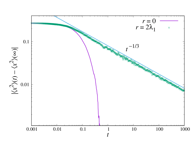
Figure 1: Simulation results of the particle with memory confined in an interval $[0,L]$ with reflecting boundary conditions. The mean square position slowly relaxes toward its asymptotic value $\langle x^{2}\rangle(t\to\infty)=L^{2}/3$ in a power-law way (symbols), while the memory-less case $r=0$ follows an exponential behaviour (purple solid line). We have set the resetting rate to $2\lambda_{1}=2D\pi^{2}/L^{2}$. The scaling law $t^{-1/3}$ predicted by Eq. (66) is displayed as a guide to the eye. We have set $L=1$, $D=1$, $x_{0}=0.25$, $dt=10^{-4}$ for the simulation time-step, and averages are performed over $10^{4}$ independent trajectories.

6 Numerical simulations

To verify and illustrate our theoretical results in the different cases, we have performed numerical simulations by incorporating resetting with memory in standard Brownian dynamics algorithms [34]. Instead of extracting the full distribution $P_{r}(x,t)$ from the simulations, we have computed the simpler mean square position of the particle $\langle x^{2}\rangle(t)$. If the position density obeys the generic form given by Eq. (4), clearly, the second moment also relaxes toward its stationary value as

$$\langle x^{2}\rangle(t)-\langle x^{2}\rangle(t\to\infty)\sim t^{-\theta_{1}}.$$ (67)

Furthermore, the single power-law decay at late time in Eq. (67) is easier to observe if the separation between $\theta_{1}$ and the exponent of the second excited mode, $\theta_{2}$, is as large as possible. In this case, the condition $t^{-\theta_{1}}\gg t^{-\theta_{2}}$ is fulfilled from shorter times in principle, and the contribution of the sub-leading terms in Eq. (39) is actually negligible.

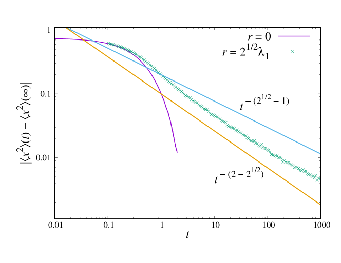
Figure 2: Relaxation of the particle with memory in a harmonic potential $U(x)=\mu x^{2}/2$. The mean square position relaxes slowly (symbols) at finite resetting rate (here $r=\sqrt{2}\lambda_{1}=\sqrt{2}\mu$). The memory-less case is shown with the purple solid line. The power-law decay of the first two leading modes, $t^{-(\sqrt{2}-1)}$ and $t^{-(2-\sqrt{2})}$, are displayed as a guide to the eye. Here, $\langle x^{2}\rangle(t\to\infty)=D/\mu$ and the stiffness is set to $\mu=1$, while $D=1$, $dt=10^{-3}$, $x_{0}=0.5$ and averages are preformed over $10^{6}$ trajectories.

For instance, for the particle confined in the box $[0,L]$, one has $\theta_{n}=\frac{D(n\pi/L)^{2}}{r+D(n\pi/L)^{2}}$ from Eq. (65) and the gap between the first two exponent reads

$$\theta_{2}-\theta_{1}=\frac{3\lambda_{1}r}{(r+4\lambda_{1})(r+\lambda_{1})}.$$ (68)

with $\lambda_{1}=D\pi^{2}/L^{2}$. Notably, fixing $\lambda_{1}$ and varying the resetting rate from 0 to $\infty$, the above quantity reaches a maximum at a value $r^{*}$ given by

$$r^{*}=2\lambda_{1},$$ (69)

while the corresponding exponents are $\theta_{1}(r^{*})=1/3$ and $\theta_{2}(r^{*})=2/3$. Simulation results are shown in Figure 1, which represents the absolute value of the difference in Eq. (67) as a function of $t$, where $\langle x^{2}\rangle(t\to\infty)=L^{2}/3$ from the uniform stationary distribution. With a resetting rate set equal to the value $r^{*}$ in Eq. (69), one indeed observes a scaling law in excellent agreement with $t^{-1/3}$ over nearly five decades, thus confirming the validity of the general expression (5). In the case $r=0$, the much faster exponential decay toward the stationary state is recovered.

For the particle confined by the harmonic potential $U(x)=\mu x^{2}/2$, the asymptotic second moment is $\langle x^{2}\rangle(t\to\infty)=D/\mu$, while $\theta_{n}=\frac{n\mu}{r+n\mu}$. The exponent gap is now given by

$$\theta_{2}-\theta_{1}=\frac{\mu r}{(r+2\mu)(r+\mu)},$$ (70)

and reaches a maximum at $r=r^{*}$ where

$$r^{*}=\sqrt{2}\mu.$$ (71)

For this value of the resetting rate, the exponents are $\theta_{1}(r^{*})=\sqrt{2}-1=0.4142...$ and $\theta_{2}(r^{*})=2-\sqrt{2}=0.5857...$ The simulation results at $r=r^{*}$ are shown in Fig. 2. Since $\theta_{1}(r^{*})$ and $\theta_{2}(r^{*})$ are closer to each other than in the box case, the agreement with the single power-law decay $t^{-\theta_{1}(r^{*})}$ is more difficult to obtain. Nevertheless, the relaxation at large $t$ is still consistent with a slow decay with an effective exponent comprised between $\theta_{1}(r^{*})$ and $\theta_{2}(r^{*})$, while the relaxation is again exponential for $r=0$.

Finally, in the case of the V-shaped potential $U(x)=F|x|$, Eq. (56) gives

$$\langle x^{2}\rangle(t)-\langle x^{2}\rangle(t\to\infty)\sim\left(\ln[(r+\lambda_{1})t]\right)^{-3/2}\,t^{-\theta_{1}},$$ (72)

and the second moment of the equilibrium distribution is $\langle x^{2}\rangle(t\to\infty)=2(D/F)^{2}$. Figure 3 displays the mean square difference in a case where $r=\lambda_{1}$, i.e., where the exponent of the leading power-law is $1/2$ according to Eq. (5). As expected, the simulation curve exhibits small deviations from a $t^{-1/2}$ law, in contrast to Fig. 1 of the box case that agrees perfectly with the predicted power-law. The logarithmic corrections in Eq. (72) are difficult to detect numerically, though; we rather measure an effective exponent of roughly $0.6$ in the last two decades.

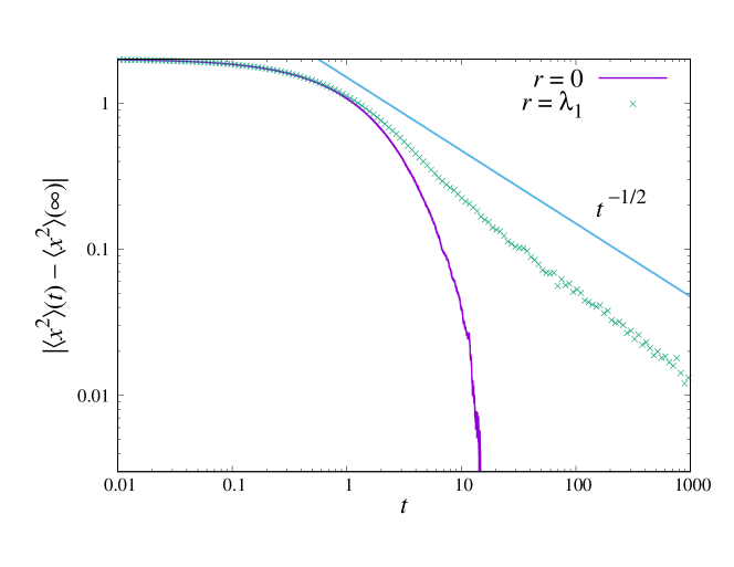
Figure 3: Relaxation of the particle with memory in the potential $U(x)=F|x|$. Symbols represent the relaxation of the mean square position for a resetting rate of $r=\lambda_{1}=F^{2}/(4D)$. The case $r=0$ is represented with the purple solid line. The power-law $t^{-1/2}$ is shown as a guide to the eye. Here, $\langle x^{2}\rangle(t\to\infty)=2(D/F)^{2}$ and the force is set to $F=1$, while $D=1$, $dt=10^{-3}$, $x_{0}=0$.

7 Summary and Conclusion

We have studied the relaxation of a Brownian particle with long range memory in confining potentials. The memory effects are introduced by stochastic resetting events, where the particle relocates to positions visited in the past, before it continues to diffuse in the potential from there. At large time, the particle’s position tends toward a steady state given by the Boltzmann-Gibbs distribution. Contrary to confined systems subject to resetting to a fixed position [23, 24, 25, 26, 27, 28, 29, 30, 31], this stationary state is in equilibrium since local detailed balance is fulfilled. Importantly, we find that the relaxation toward the steady state is not exponential in time like in standard Brownian motion but follows an inverse power-law, for any non-zero value of the resetting rate. This sluggish decay is a consequence of the preferential character of memory in the model, where more frequently visited sites are more likely to be visited again in the future. Consequently, the particle tends to stay close to its starting point and takes a very long time to visit the accessible positions.

The exponent that controls the slow relaxation can be obtained exactly and lies in the interval $(0,1)$. It depends on the resetting rate and on the longest relaxation time $1/\lambda_{1}$ of the memory-less particle, through a simple general formula given by Eq. (5). In other words, knowing the asymptotic exponential relaxation of the standard Brownian particle in a potential $U(x)$ allows us to predict the anomalous decay in the presence of memory for any value of the resetting rate. We have applied our theory to several analytically tractable potentials (box, harmonic, V-shaped), finding very good agreement with simulations. The scale-free dynamics at large $t$ is generic and can be compared to a self-organised critical state, independent of the initial position and characterised by a non-universal exponent.

Our model represents a simple description of the movements of an animal in its home range, i.e., a limited region of space that can be produced by an effective confining potential [18], but where in addition to random motion, the living organism chooses from time to time to revisit familiar places. Empirically, space use by animals is known to be highly heterogeneous even within limited areas [35, 1], a feature qualitatively captured by our finding that the exploration of a small accessible region can be very slow. It would be interesting to extend the model to situations where the external potential has a local minimum and to study the crossing of the particle over a barrier.

References

References

- [1] Boyer D and Solis-Salas C 2014 Random walks with preferential relocations to places visited in the past and their application to biology Phys. Rev. Lett. 112 240601.
- [2] Boyer D, Evans M R and Majumdar S N 2017 Long time scaling behaviour for diffusion with resetting and memory J. Stat. Mech. 023208.
- [3] Evans M R and Majumdar S N 2011 Diffusion with stochastic resetting Phys. Rev. Lett. 106 160601.
- [4] Evans M R, Majumdar S N and Schehr G 2020 Stochastic resetting and applications J. Phys. A: Math. Theor. 53 193001.
- [5] Majumdar S N, Sabhapandit S and Schehr G 2015 Dynamical transition in the temporal relaxation of stochastic processes under resetting Phys. Rev. E 91 052131.
- [6] Boyer D and Romo-Cruz J C R 2014 Solvable random walk model with memory and its relations with Markovian models of anomalous diffusion Phys. Rev. E 90 042136.
- [7] Boyer D and Pineda I 2016 Slow Lévy flights Phys. Rev. E 93 022103.
- [8] Boyer D and Majumdar S N 2024 Active particle in one dimension subjected to resetting with memory Phys. Rev. E 109 054105.
- [9] Mailler C and Uribe-Bravo G 2019 Random walks with preferential relocations and fading memory: a study through random recursive trees J. Stat. Mech. 093206.
- [10] Boci E-S and Mailler C 2023 Large deviation principle for a stochastic process with random reinforced relocations J. Stat. Mech. 083206.
- [11] Börger L, Dalziel B D and Fryxell J M 2008 Are there general mechanisms of animal home range behaviour? A review and prospects for future research Ecol. Lett. 11 637.
- [12] Fryxell J M, Hazell M, Börger L, Dalziel B D, Haydon D T, Morales J M, McIntosh T and Rosatte R C 2008 Multiple movement modes by large herbivores at multiple spatiotemporal scales Proc. Natl. Acad. Sci. 105 19114.
- [13] van Moorter B, Visscher D, Benhamou S, Börger L, Boyce M S and Gaillard J-M 2009 Memory keeps you at home: a mechanistic model for home range emergence Oikos 118 641.
- [14] Fagan W F, Lewis M A, Auger-Méthé M, Avgar T, Benhamou S, Breed G, LaDage L, Schlägel U E, Tang W-w, Papastamatiou Y P, Forester J and Mueller T 2013 Spatial memory and animal movement Ecol. Lett. 16 1316.
- [15] Merkle J, Fortin D and Morales J M 2014 A memory-based foraging tactic reveals an adaptive mechanism for restricted space use Ecol. Lett. 17 924.
- [16] Fagan W F, McBride F and Koralov L 2023 Reinforced diffusions as models of memory-mediated animal movement J. R. Soc. Interface. 20 20220700.
- [17] Falcón-Cortés A, Boyer D, Merrill E, Frair J L and Morales J M 2021 Hierarchical, memory-based movement models for translocated elk (Cervus canadensis) Front. Ecol. Evol. 9 702925.
- [18] Moorcroft P R and Lewis M A 2006 Mechanistic Home Range Analysis (Princeton University Press, Princeton).
- [19] Fagan W F, Gurarie E, Bewick S, Howard A, Cantrell R S and Cosner C 2017 Perceptual ranges, information gathering, and foraging success in dynamic landscapes Am. Nat. 189 474.
- [20] Martinez-Garcia R, Fleming C H, Seppelt R, Fagan W F and Calabrese J M 2020 How range residency and long-range perception change encounter rates J. Theor. Biol. 498 110267.
- [21] Fagan W F, Saborio C, Hoffman T D, Gurarie E, Cantrell R S and Cosner C 2022 What’s in a resource gradient? Comparing alternative cues for foraging in dynamic environments via movement, perception, and memory Theor. Ecol. 15 267.
- [22] Risken H 1996 The Fokker-Planck Rquation: Methods of Solutions and Applications (Springer-Verlag, Berlin).
- [23] Pal A 2015 Diffusion in a potential landscape with stochastic resetting Phys. Rev. E 91 012113.
- [24] Ahmad S, Nayak I, Bansal A, Nandi A and Das D 2019 First passage of a particle in a potential under stochastic resetting: A vanishing transition of optimal resetting rate Phys. Rev. E 99 022130.
- [25] Mercado-Vásquez G, Boyer D, Majumdar S N and Schehr G 2020 Intermittent resetting potentials J. Stat. Mech. 113203.
- [26] Gupta D, Plata C A, Kundu A and Pal A 2020 Stochastic resetting with stochastic returns using external trap J. Phys. A: Math. Theor. 54 025003.
- [27] Capala K, Dybiec B and Gudowska-Nowak E 2021 Dichotomous flow with thermal diffusion and stochastic resetting Chaos 31 053132.
- [28] Ray S and Reuveni S 2021 Resetting transition is governed by an interplay between thermal and potential energy J. Chem. Phys. 154 171103.
- [29] Ahmad S, Rijal K and Das D 2022 First passage in the presence of stochastic resetting and a potential barrier Phys. Rev. E 105 044134.
- [30] Ahmad S and Das D 2023 Comparing the roles of time overhead and spatial dimensions on optimal resetting rate vanishing transitions, in Brownian processes with potential bias and stochastic resetting J. Phys. A: Math. Theor. 56 104001.
- [31] Jain S, Boyer D, Pal A and Dagdug L 2023 Fick–Jacobs description and first passage dynamics for diffusion in a channel under stochastic resetting J. Chem. Phys. 158 054113.
- [32] Sabhapandit S and Majumdar S N 2020 Freezing transition in the barrier crossing rate of a diffusing particle Phys. Rev. Lett. 125 200601 and references therein.
- [33] Handbook of Mathematical Functions with Formulas, Graphs, and Mathematical Tables 1965 edited by Abramowitz M and Stegun I A (Dover, New York).
- [34] Dagdug L, Peña J and Pompa-García I 2024 Diffusion Under Confinement, a Journey Through Counterintuition (Springer, Cham).
- [35] Russo S E, Portnoy S and Augspurger C K 2006 Incorporating animal behavior into seed dispersal models: implications for seed shadows Ecology 87 3160.