GKLS Vector Field Dynamics for Gaussian States

Abstract

Abstrasct: We construct the vector field associated to the GKLS generator for systems described by Gaussian states . This vector field is defined on the dual space of the algebra of operators, restricted to operators quadratic in position and momentum. It is shown that the GKLS dynamics accepts a decomposition principle, that is, this vector field can be decomposed in three parts, a conservative Hamiltonian component, a gradient-like, and a Choi–Krauss vector field. The two last terms are considered a “perturbation” associated with dissipation. Examples are presented for a harmonic oscillator with different dissipation terms.

Keywords: Open quantum systems; Quantum dissipative dynamics; Gaussian states; Non-unitary evolution; Statistical mix states.

I Motivation and previous works

The geometric formulation of quantum mechanics makes use of structures and methods used in classical dynamics and in a lesser way of those appearing in the theory of general relativity, suggesting a powerful framework for approaching both, the conceptual and the mathematical foundations of quantum mechanics. Such a geometric approach consists in describing all the fundamental properties of the quantum theory through the use of geometric structures on an appropriate classical manifold.

This perspective of the quantum theory was formally introduced by the pioneering works of Strocchi Strocchi-1966 , Cantoni Cantoni-1978 , Kramer–Saraceno Kramer-1980 and Cirelli–Lanzavecchia–Mania Cirelli-1983 . Strocchi realized that the space of expectation values for Hamiltonian systems quadratic in position and momentum, allows to introduce a set of complex coordinates and to obtain a “classical” form of quantum mechanics, establishing a direct connection between Poisson brackets and commutators as well as between canonical transformations that preserve the Jordan product and the unitary representation of operators.

Following the idea of a “classical” form of quantum mechanics proposed by Strocchi, it was soon recognized that for Hamiltonian systems with a group structure $G$, i.e. the Hamiltonian is written in terms of a generators of a Lie algebra ${\mathfrak{D}}_{G}$, it is possible to define a dual Lie algebra ${\mathfrak{D}}_{G}^{\ast}$ of linear functions which are related to the observables associated to the operators in ${\mathfrak{D}}_{G}$; see Ref. Kramer-1980 ; Moshinsky-1971 ; Mello-1975 and references therein. The operator basis satisfies a set of commutation relations while the linear functions a set of corresponding Poisson brackets. The geometry of the dual Lie algebra ${\mathfrak{D}}^{\ast}_{G}$ is described by the symplectic structures on orbits under $G$, which are characterized as submanifolds of ${\mathfrak{D}}_{G}$ given by the quotient space $G/H_{s}$, with $H_{s}$ the stability group of the fiducial state. By considering coherent states of the Lie group $G$, one arrives at symplectic submanifolds to describe the corresponding “classical” Hamiltonian evolution, which in general is integrable.

On the other hand, the geometrical study of quantum mechanics by Cirelli–Lanzavecchia–Mania is motivated by the physically equivalent description of a quantum system by means of the Hilbert space ${\mathcal{H}}$ or by its projective Hilbert space ${\cal PH}$. Let us recall that Hilbert spaces ${\cal H}$ were introduced by Dirac as a consequence of the linear superposition principle for wave functions satisfying the interference phenomena Dirac-1981 ; however, the arbitrary global phase of the wave functions leads to the ray concept (an equivalence class of wave functions) and the definition of the projective Hilbert space ${\cal PH}$. Then, in Ref. Cirelli-1983 it was shown that, the projective space of a complex Hilbert space is a Kähler manifold and also the set of pure states of the von Neumann algebra, thus showing a link between these structures. This natural Kähler structure is defined by a symplectic form, a Riemannian metric called the Fubini-Study metric and a complex structure on the manifold of pure states.

Nowadays, there is a growing interest in the geometric description of open quantum systems and their dynamics; specifically, there has been great advances in the geometric study of the general master equation governing the Markovian dynamics of finite quantum systems Grabowski-2005 ; Aniello-2011 ; Ciaglia-2017 ; Chruscinski-2019 . From here onward, we restrict our considerations to finite dimensional Hilbert spaces. Following Ciaglia-2017 , we can establish the kinematics for the $n$-levels quantum systems. In this case, we are dealing with systems whose observables are elements of a finite $C^{\ast}$-algebra, i.e., being $\mathcal{M}_{n}({\mathbb{C}})$ the $C^{\ast}$-algebra of $(n\times n)$ complex matrices, then the observables are elements of the finite algebra ${\mathfrak{A}}_{n}=\mathcal{M}_{n}({\mathbb{C}})$, for $n\geq 2$.

Thus, the space of observables ${\mathfrak{D}}_{n}$ is identified with the subset of ${\mathfrak{A}}_{n}$ consisting of self-adjoint elements, i.e. ${\mathfrak{D}}_{n}\subset{\mathfrak{A}}_{n}$. In addition, ${\mathfrak{A}}_{n}$ possess a natural Hilbert inner product $\langle\hat{a}\,,\,\hat{b}\rangle:={\rm Tr}\{\hat{a}^{\dagger}\hat{b}\}$ and hence ${\mathfrak{A}}_{n}$ is a complex Hilbert space. If ${\mathfrak{A}}^{\ast}_{n}$ is the dual algebra of ${\mathfrak{A}}_{n}$, it is known that for every $\xi\in{\mathfrak{A}}^{\ast}_{n}$ there is a unique $\hat{\xi}\in{\mathfrak{A}}_{n}$ such that $\xi(\hat{a})=\langle\hat{\xi}\,,\,\hat{a}\rangle$ for all $\hat{a}\in{\mathfrak{A}}_{n}$; then, the space of states $\mathcal{S}$ of ${\mathfrak{A}}_{n}$ is defined as

$${\mathcal{S}}:=\{\rho\in{\mathfrak{D}}_{n}^{\ast}\subset{\mathfrak{A}}_{n}^{\ast}\,|\,\rho(\hat{a}\hat{a}^{\dagger})\geq 0,\rho(\hat{\mathbb{I}})=1\}\,,$$ (1)

where $\mathbb{I}\in{\mathfrak{A}}_{n}$ is the identity operator and ${\hat{a}}\in{\mathfrak{D}}_{n}$. Therefore, for each quantum state $\xi\equiv\rho\in{\mathfrak{A}}_{n}^{\ast}$ there is a corresponding $\hat{\rho}\in{\mathfrak{A}}_{n}$ defined as the self-adjoint semi-positive matrix such that ${\rm Tr}\{\hat{\rho}\,\hat{\mathbb{I}}\}=1$, meaning that $\hat{\rho}$ is a density operator. Furthermore, from the one-to-one correspondence between elements of ${\mathfrak{D}}_{n}^{\ast}$ and elements of ${\mathfrak{D}}_{n}$, it follows that ${\mathcal{S}}$ may be decomposed as

$${\mathcal{S}}=\bigsqcup_{r=1}^{n}{\mathcal{S}}_{r}\,,$$ (2)

with

$${\mathcal{S}}_{r}=\{\rho\in{\mathcal{S}}\,|\,\text{rank}(\rho)=r\}\,,$$ (3)

where $\text{rank}(\rho)$ denotes the rank of $\rho$ defined as the matrix rank of the density matrix $\hat{\rho}\in{\mathfrak{D}}_{n}$. Then, as has been shown in Refs. Ciaglia-2017 ; Chruscinski-2019 , ${\mathcal{S}}_{r}$ is a homegeneous space of the Lie group

$$SL({\mathfrak{A}}_{n}):=\{g\in{\mathfrak{A}}_{n}|\det(g)=1\}\,,$$ (4)

and therefore is a differential manifold, in those references, it is also proved that on each ${\mathcal{S}}_{k}$ there is an action of the compact Lie subgroup

$$SU({\mathfrak{A}}_{n}):=\{\mathbf{U}\in{\mathfrak{A}}_{n}|\mathbf{U}\mathbf{U}^{\dagger}=\mathbb{I},\det(\mathbf{U})=1\}\,,$$ (5)

where $SU({\mathfrak{A}}_{n})\subset SL({\mathfrak{A}}_{n})$ and the orbits of this action are known in quantum theory as isospectral manifolds. In particular, the manifold of pure states, i.e. $\text{rank}(\rho)=1$, turns out to be a homogeneous space for $SU({\mathfrak{A}}_{n})$ and $SL({\mathfrak{A}}_{n})$.

Once the manifold of states is characterized, relevant geometric structures can be introduced. Each isospectral manifold is endowed with a Kähler structure, thus, through the symplectic form, it is possible to define a Hamiltonian dynamics on these manifolds which corresponds to the unitary evolution, see Refs. Grabowski-2005 ; Ciaglia-2017 . In this work, we will introduce more general geometric structures on ${\mathcal{S}}$, so a more general dynamical evolution can be defined than the symplectic one. This new dynamics is defined for the entire manifold of states, hence it represents the evolution of open quantum systems. For instance, the dynamics associated with the Markovian evolution introduced in Refs. Gorini-1976 ; Lindblad-1976 by means of the Gorini–Kossakowski–Lindblad–Sudarshan (GKLS) master equation

$$L(\hat{\rho})=-\frac{{\rm i}}{\hbar}[\hat{H},\hat{\rho}]_{-}-\frac{1}{2}\sum^{3}_{j}[\hat{v}^{\dagger}_{j}\,\hat{v}_{j},\hat{\rho}]_{+}+\sum^{3}_{j}\hat{v}^{\dagger}_{j}\,\hat{\rho}\,\hat{v}_{j}\,,$$ (6)

where $\hat{\rho}$ is the density operator associated to a quantum state $\rho\in{\mathcal{S}}$, $\hat{H}\in{\mathfrak{D}}_{n}$ is the Hamiltonian operator and $\hat{v}_{j}\in{\mathfrak{A}}_{n}$ is an operator introducing dissipation to the system; here, $[\,\cdot\,,\,\cdot\,]_{-}$ and $[\,\cdot\,,\,\cdot\,]_{+}$ denote the commutator and the anti-commutator in ${\mathfrak{A}}_{n}$. The geometric description of the GKLS master equation means to describe the GKLS equation of motion through a vector field $\Gamma$ in the affine space ${\mathfrak{T}}_{n}^{1}\subset{\mathfrak{D}}^{\ast}_{n}$ defined as

$${\mathfrak{T}}_{n}^{1}=\{\xi\in{\mathfrak{D}}_{n}^{\ast}\,|\,{\rm Tr}\{\hat{\xi}\,\mathbb{I}\}=1\}\,.$$ (7)

From the Lie–Jordan algebra structure of ${\mathfrak{D}}_{n}$ it is shown in Ref. Ciaglia-2017 that the affine vector field $\Gamma$ can decomposed as

$$\Gamma=X_{H}+Y_{b}+Z_{\mathcal{K}}\,,$$ (8)

where $X_{H}$ is the Hamiltonian vector field associated with the first term of the GKLS generator in (6) and $Y_{b}+Z_{\mathcal{K}}$ are related to the dissipative part of the GKLS generator given by the second and third terms in (6). Then, the Hamiltonian vector fields are tangent to ${\mathfrak{T}}_{n}^{1}$, more precisely, they are tangent to the manifolds of quantum states with fixed rank. On the other hand, the vector field $Y_{b}+Z_{\mathcal{K}}$ generates a dynamical evolution that changes the rank and the spectrum of the density matrix, that is, it represents a dissipation term in the dynamics.

There are two types of systems in what refers to the encoding of the quantum information: i) systems with a finite spectrum, i.e. in the form of q-bits or q-dits and ii) systems with an infinite spectrum such as those given in the form of the position or momentum representations. For instance, one may consider Gaussian states that emerge naturally in Hamiltonians quadratic in the position and momentum variables Malkin-1969 ; Malkin-1973 , or those associated with Hamiltonians which are described employing algebraic structures whose states are called generalized coherent states Perelomov-1972 ; Arecchi-1972 ; Onofri-1975 . All of them, even the non-linear coherent states Manko-1997 ; Aniello-2000 ; Aniello-2009 ; Cruz-2021 , constitute examples of quantum states whose properties may be described by finite-dimensional smooth manifolds.

In particular, the generalized coherent states solutions to the Schrödinger equation for Hamiltonians quadratic in the position and momentum operators, have been extensively studied due to their broad application in quantum optics and quantum technologies. In these cases, one may express the density matrix in the position representation in the general form

$$\langle q^{\prime}|\,\hat{\rho}\,|q\rangle=\frac{1}{\sqrt{2\,\pi\,\sigma^{2}_{q}}}\exp\Bigg{\{}\frac{1}{2\,\sigma^{2}_{q}}\left[\frac{\sigma_{qp}}{\hbar}(q-q^{\prime})-\frac{{\rm i}}{2}\,(q+q^{\prime}-2\langle\hat{q}\rangle)\right]^{2}-\frac{\sigma^{2}_{p}}{2\,\hbar^{2}}(q-q^{\prime})^{2}+\frac{{\rm i}}{\hbar}\,\langle\hat{p}\rangle\,(q-q^{\prime})\Bigg{\}}\,,$$ (9)

which corresponds to a Gaussian density matrix. These normalized positive functional are parametrized by the first $(\langle\hat{q}\rangle,\langle\hat{p}\rangle)$ and second $(\sigma_{q}^{2},\sigma_{p}^{2},\sigma_{qp})$ moments. The second moments are constrained by the saturated Robertson–Schrödinger uncertainty relation, i.e., $\sigma_{q}^{2}\sigma_{p}^{2}-\sigma^{2}_{qp}=\frac{\hbar}{4}$. The first and second moments parametrize the space of states defining a finite-dimensional manifold with a quantum evolution that can be described through a symplectic evolution, for details see Ref. Cruz-2021 .

For the Gaussian density matrix given in (9) is possible to construct the GKLS dynamical vector field $\Gamma$ defined in the space of parameters, which accepts the decomposition as the vector field in (8). To see this, notice that the density matrix in (9) can describe non-pure states, as has been remarked in Ref. Ferraro-2005 , where the degree of purity is given by a parameter $r\in[1,\infty)$, such that

$${\rm Tr}\{\hat{\rho}^{2}\}=\frac{1}{r}\quad\text{and}\quad\sigma_{q}^{2}\,\sigma_{p}^{2}-\sigma^{2}_{qp}=\frac{\hbar^{2}\,r^{2}}{4}\,.$$ (10)

Consequently, for $r=1$ we have pure states and only in this case, the density operator can be factorized as $\hat{\rho}=|\alpha\rangle\langle\alpha|$, where $|\alpha\rangle$ is the so-called generalized coherent state. In this form, the GKLS dynamics acting on the Gaussian states can modify the parameter $r$ introducing a change of purity. An expression for the Gaussian state that explicitly depends on the parameter $r$ is obtained by its Wigner representation given by the quasi-distribution function

$$W_{r}(q,p)=\frac{1}{\pi\,\hbar\,r}\exp\left\{-\frac{2}{\hbar^{2}\,r^{2}}\left[\sigma_{p}^{2}q^{2}-2\sigma_{qp}qp+\sigma_{q}^{2}p^{2}\right]\right\}\,.$$ (11)

From this expression, we observe that the change in the degree of purity of the state is reflected in the form of the Wigner function, having an explicit dependence on the $r$-parameter.

In this work, we aimed to find the GKLS vector field for Gaussian states, which allows a change in the degree of purity through the variation of the $r$-parameter. Nevertheless, trying to follow the same procedure presented in Ciaglia-2017 , it is immediate to notice that the infinite representation in (9) for Gaussian states results inappropriate for such a task. In the q-bit case, it is well known that states described by $\rho$ can be mapped to points in a ball $\mathbf{B}$ of radius one. Then, the GKLS dynamics dictated by the master equation (6) for the operator $\hat{\rho}$ induces a GKLS vector field $\Gamma$ which determines the dynamical evolution of states. Therefore, one may notice that deducing the GKLS dynamics for Gaussian states following this procedure is not straightforward as such states do not possess a finite-dimensional representation. However, an interesting observation can be made: there is a one-to-one correspondence between Gaussian states in the Hilbert space and points in the finite-dimensional space of parameters. Therefore, restricting our problem to Gaussian states with vanishing first moments, the space of parameters is the solid hyperboloid

$$\mathbf{H}=\{(y^{1},y^{2},y^{3})\in{\mathbb{R}}^{3}\,|\,(y^{1})^{2}-(y^{2})^{2}-(y^{3})^{2}\geq 1\}\,,$$ (12)

where $(y^{1},y^{2},y^{3})$ are related to the second moments by

$$y^{1}=\frac{1}{\hbar}(\sigma^{2}_{p}+\sigma^{2}_{q})\,,\qquad y^{2}=\frac{2}{\hbar}\,\sigma_{qp}\,,\qquad y^{3}=\frac{1}{\hbar}(\sigma^{2}_{p}-\sigma^{2}_{q}).$$ (13)

Then, there is a clear analogy between the ball $\mathbf{B}$ for the q-bit states, and the solid hyperboloid $\mathbf{H}$ for Gaussian states, in the sense that quantum states are represented as points in these finite manifolds. Furthermore, while on $\mathbf{B}$ there is a natural action of the $SU(2)$ Lie group, in $\mathbf{H}$ there is a smooth action of the $SL(2,{\mathbb{R}})$ Lie group. This fact allows to definine the immersion of the space of $(2\times 2)$-matrices into the space of parameters $\mathbf{H}$, i.e.,

$$m:\mathcal{M}_{2}\to\mathbf{H}\qquad\text{that is}\qquad\xi\mapsto(y^{1},y^{2},y^{3}),$$ (14)

where $\xi$ is an element of the Lie algebra $sl(2,{\mathbb{R}})^{\ast}$, note that $\xi$ is not a state. Using this immersion the evolution in the space of matrices determines the dynamics in the space of parameters and consequently, for the Gaussian states. As we will show, this allows us to follow the same procedure proposed for the $n$-level systems presented in Ciaglia-2017 .

Now. to ensure that the dynamics is the one associated to the GKLS generator (6), we restrict our problem to only consider operators which are quadratic in the position and momentum operator such that they are elements of the ${\mathfrak{sl}}(2,{\mathbb{R}})$ Lie algebra. As it is well-known, ${\mathfrak{sl}}(2,{\mathbb{R}})$ accepts a $(2\times 2)$-matrix representation, an important feature for our purposes. Then, we claim that the GKLS evolution for $\hat{\xi}$ can be determined through the master equation

$$L(\hat{\xi})=-\frac{{\rm i}}{\hbar}[\hat{H},\hat{\xi}]_{-}-\frac{1}{2}\sum^{3}_{j}[\hat{v}^{\dagger}_{j}\,\hat{v}_{j},\hat{\xi}]_{+}+\sum^{3}_{j}\hat{v}^{\dagger}_{j}\,\hat{\xi}\,\hat{v}_{j}\,,$$ (15)

where $\hat{H}$ and $\hat{v}$ are elements of ${\mathfrak{sl}}(2,{\mathbb{R}})$ and, consequently, they can represent by $(2\times 2)$-matrices. Therefore, we can follow the same procedure for the q-bit system considered in Ref. Ciaglia-2017 , up to the appropriate modifications, to obtain the GKLS vector field for the Gaussian states.

The paper is organized as follows. In Section II we review the case of one q-bit systems, starting with the description of the space of quantum states as a manifold with boundary and establishing its kinematic properties, in particular, we describe its foliation in terms of two-spheres. In Subsection II.1, we describe the Hamiltonian dynamics on each isospectral submanifold through its Kähler structure. In Subsection II.2, we analyze the quantum systems from the point of view of observables and use the Lie-Jordan algebra to define the two relevant geometric structures, a skew-symmetric bivector field which defines a Poisson structure for the space of functions on the dual algebra, that is associated to the Lie product and a symmetric bivector field which defines a symmetric product, both are realizations of the algebra on the space of linear functions. In Subsection II.3, we construct the GKLS vector field and find the decomposition (8), to do so, we perform a reduction procedure and find the Choi-Kraus vector field associated to the completely positive map $\mathcal{K}$ in (6). In the last subsection, II.4, we present two examples for a damping process of a two-level system. In Section III, and its subsections, our main results are presented, where the procedure reviewed in Section II, with the appropriate tuning, is used to determine the GKLS vector field for the Gaussian states. It is worth to mention that, adapting the procedure to an infinite-dimensional state space is not straightforward, and some modifications had to be considered. Finally, in Section IV, we present our conclusions and some of the lines of research that will be presented in a set of future works.

II On the kinematics and dynamics of Dissipative one $q$-bit systems

In this section, the GKLS dynamical vector field for one $q$-bit systems is constructed in detail to exemplify the ideas that we will apply in section III for the Gaussian density matrices. It is well known that in general, the quantum space for the $q$-bit can be immersed in the space of $2\times 2$ Hermitian matrices, where the basis may be provided by the Pauli matrices

$$\sigma_{1}=\left(\begin{array}[]{c c}0&1\\ 1&0\end{array}\right)\,,\quad\sigma_{2}=\left(\begin{array}[]{c c}0&-{\rm i}\\ {\rm i}&0\end{array}\right)\,,\quad\sigma_{3}=\left(\begin{array}[]{c c}1&0\\ 0&-1\end{array}\right)\,,$$ (16)

and the identity matrix

$$\sigma_{0}=\left(\begin{array}[]{c c}1&0\\ 0&1\end{array}\right)\,.$$ (17)

Thus, an arbitrary density matrix may be expressed as

$$\rho=\frac{1}{2}(\sigma_{0}+x^{k}\sigma_{k})=\frac{1}{2}\,x^{\mu}\,\sigma_{\mu}\,,$$ (18)

where $k=1,2,3$, $\mu=0,1,2,3$ and from the normalization condition ${\rm Tr}\{\hat{\rho}\,\hat{\sigma}^{0}\}=1$ it follows that $x^{0}=1$. In this expression, and from here on, Einstein’s summation convention over repeated indices is assumed. Thus, for example, every pure quantum state is represented by a point $(x^{1},x^{2},x^{3})$ in the unit sphere, such that $x^{k}~{}=~{}{\rm Tr}\{\hat{\sigma}^{k}\hat{\rho}\}$. Here the purity condition $\rho^{2}=\rho$ defines the unit sphere

$$S^{2}=\{(x^{1},x^{2},x^{3})\in{\mathbb{R}}^{3}\,|\,(x^{1})^{2}+(x^{2})^{2}+(x^{3})^{2}=1\}\,,$$ (19)

which is known as the Bloch sphere. On the other hand, for mixed states one has that the mixture condition ${\rm Tr}\{\hat{\rho}^{2}\}<1$ defines the constraint

$$(x^{1})^{2}+(x^{2})^{2}+(x^{3})^{2}<1\,,$$ (20)

where the maximal mixed state correspond to $x^{1}=x^{2}=x^{3}=0$. Therefore, a $q$-bit state may be always represented by a point $\mathbf{x}=(x^{1},x^{2},x^{3})$ on the solid ball

$$\mathbf{B}=\{(x^{1},x^{2},x^{3})\in{\mathbb{R}}^{3}\,|\,(x^{1})^{2}+(x^{2})^{2}+(x^{3})^{2}\leq 1\}\,.$$ (21)

In the literature, the points $\mathbf{x}\in\mathbf{B}$ are called Bloch vectors or polarization vectors Scully-1999 . The space of 2-level quantum system is made up of two strata: $\mathcal{S}_{1}$ by unit sphere $S^{2}$, the space of pure states and $\mathcal{S}_{2}$ the open interior of the ball, space of mix states. Therefore, the quantum space of q-bit systems is a manifold with boundary.

As a final remark, let us notice that the manifold $\mathbf{B}$ is a foliated space, i.e.,

$$\mathbf{B}=\bigcup_{r\in[0,1]}\ell_{r}$$ (22)

where the leaves of the foliation correspond to

$$\ell_{r}=\{(x^{1},x^{2},x^{3})\in{\mathbb{R}}^{3}\,|\,(x^{1})^{2}+(x^{2})^{2}+(x^{3})^{2}=r^{2},r\leq 1\}\,.$$ (23)

A schematic picture of this foliation is displayed in Fig. 1. It is important to note that we have a singular foliation, i.e., the leaves are not all of the same dimension, having a singular point at the origin. Nevertheless, removing the origin one has a regular foliation given by the family $\{\ell_{r}\}$ of disjoint subsets, with $r\in(0,1]$ and where $\ell_{r}$ are the leaves of the foliation, on which a differential structure can be given. In general, this foliation is a consequence of the smooth action of $SU({\mathfrak{A}}_{2})$. In the literature, the leaves of this foliation are the so-called manifolds of isospectral states Ciaglia-2017 ; Chruscinski-2019 .

Figure 1: Pictorial representation of the space of quantum states for the $q$-bit systems. A quantum state is represented by a point $\mathbf{x}=(x^{1},x^{2},x^{3})$ in the ball $\mathbf{B}$. In addition, one may see that the ball is foliated by a disjoint family of spheres $\ell_{r}$.

II.1 Dynamical study of one q-bit systems from a state point of view

Once we have introduced the manifolds of isospectal states in this section, we procede to define the symplectic dynamics and the gradient vector field on these manifolds. To do that, let us note that each manifold of isospectral states is endowed with a Kähler structure, i.e., there is a symplectic form $\omega_{\tiny\mbox{FS}}$, a Riemannian metric $g_{\tiny\mbox{FS}}$, known as the Fubini–Study metric, and a complex structure $J$ all of them defined globally on each isospectral manifold Grabowski-2005 ; Ercolessi-2010 ; Cruz-2020 . Moreover, the symplectic form and the Riemannian metric define a Hamiltonian vector field $\mathbb{X}_{H}$ and a gradient vector field $\mathbb{Y}_{H}$. Given a real function $f_{\hat{H}}\in{\mathfrak{D}}^{\ast}_{2}$ defined as the expectation value of the observable $\hat{H}\in{\mathfrak{D}}_{2}$, that is,

$$f_{\hat{H}}:={\rm Tr}\{\hat{\rho}\,\hat{H}\}\,,$$ (24)

then the Hamiltonian vector field and the gradient vector field are defined intrinsically by

$$\omega_{\tiny\mbox{FS}}(\mathbb{X}_{H},\,\cdot\,)={\rm d}f_{\hat{H}}\quad\text{and}\quad g_{\tiny\mbox{FS}}(\mathbb{Y}_{H},\,\cdot\,)={\rm d}f_{\hat{H}}\,,$$ (25)

respectively, along with the property

$$J(\mathbb{X}_{H})=\mathbb{Y}_{H}\,,$$ (26)

which provides an intrinsic definition of the complex structure tensor $J$.

To give the coordinates expression for all these definitions, let us consider the coordinate charts $(U_{1},\phi_{1})$, $(U_{2},\phi_{2})$ for the foliation $\ell_{r}$, with $U_{1},U_{2}\subset\ell_{r}$ and

$$\phi_{1}:U_{1}\to{\mathbb{C}}:(x^{1},x^{2},x^{3})\mapsto z\quad,\quad\phi_{2}:U_{2}\to{\mathbb{C}}:(x^{1},x^{2},x^{3})\mapsto\zeta\,,$$ (27)

where the complex parameters $z$ and $\zeta$ are given by

$$z=\frac{x^{1}-{\rm i}x^{2}}{r-x^{3}}\,,\qquad\zeta=\frac{x^{1}+{\rm i}x^{2}}{r+x^{3}}\,.$$ (28)

In this manner, the set $\{(U_{1},\phi_{1}),(U_{2},\phi_{2})\}$ constitutes an atlas for each foliation $\ell_{r}$. These coordinates in quantum mechanics are employed in to describe atomic coherent states Arecchi-1972 or spin coherent states Radcliffe-1971 , see also Perelomov-1977 ; Zhang-1990 .

Geometrically, by considering $\{(U_{1},\phi_{1}),(U_{2},\phi_{2})\}$ corresponds to the stereographic projection from the “north pole” and the “south pole” of the sphere onto the equatorial plane, respectively. Notice that, using the Cartesian coordinates $(x^{1},x^{2},x^{3})$ we are giving an extrinsic geometric description of the system, in which case one obtains linear equations of motion. On the other hand, the stereographic projection atlas constitutes an intrinsic geometric description and, as we will see, the equations of motions are non-linear.

Now, in the coordinate chart $(U_{1},\phi_{1})$ the symplectic form and the Riemannian metric are given by

$$\omega_{\tiny\mbox{FS}}=\frac{-{\rm i}\,\hbar\,r^{2}}{(1+\bar{z}z)^{2}}{\rm d}\bar{z}\,\wedge\,{\rm d}z\,,\quad\text{and}\quad g_{\tiny\mbox{FS}}=\frac{-\hbar\,r^{2}}{(1+\bar{z}z)^{2}}{\rm d}\bar{z}\,\otimes_{\tiny\mbox{s}}\,{\rm d}z\,,$$ (29)

respectively. In these definitions one considers the wedge product ${\rm d}\bar{z}\,\wedge\,{\rm d}z={\rm d}\bar{z}\otimes{\rm d}z-{\rm d}z\otimes{\rm d}\bar{z}$ together with the symmetrical product ${\rm d}\bar{z}\,\otimes_{\tiny\mbox{s}}\,{\rm d}z={\rm d}\bar{z}\otimes{\rm d}z+{\rm d}z\otimes{\rm d}\bar{z}$, while the complex structure has the form

$$J_{\tiny\mbox{FS}}=\frac{1}{{\rm i}}\left({\rm d}z\otimes\frac{\partial}{\partial z}-{\rm d}\bar{z}\otimes\frac{\partial}{\partial\bar{z}}\right)\,.$$ (30)

To express the density matrix (18) in this coordinate system, one has to take into account the inverse of the stereographic projection to obtain the relations

$$x^{1}=r\frac{z+\bar{z}}{1+z\bar{z}}\,,\quad x^{2}=-\frac{r}{{\rm i}}\frac{z-\bar{z}}{1+z\bar{z}}\quad\text{and}\quad x^{3}=r\frac{z\bar{z}-1}{1+z\bar{z}}\,,$$ (31)

and then, by direct substitution, the density matrix has the form

$$\rho=\frac{1}{1+\bar{z}z}\left(\begin{array}[]{ccc}\frac{1}{2}(1-r)+\frac{1}{2}(1+r)\bar{z}z&r\,z\\ &\\ r\,\bar{z}&\frac{1}{2}(1+r)+\frac{1}{2}(1-r)\bar{z}z\\ \end{array}\right)\,,$$ (32)

where the dependence on the $r$-parameter is explicit. From density matrix expressed in Eq. (32), the expectation value of an arbitrary observable operator can be obtained. In general, a self-adjoint operator can be written as $\hat{H}=H_{\mu}\,\hat{\sigma}^{\mu}$; thus, its expectation value corresponds to

$$f_{\hat{H}}:={\rm Tr}\{\hat{\rho}\,\hat{H}\}=H_{0}+H_{k}x^{k}\,,$$ (33)

and taking into account the transformations in (31), it can be expressed as

$$f_{\hat{H}}=\frac{1}{1+\bar{z}z}\left[(H_{0}+r\,H_{3})z\bar{z}+r(H_{1}+{\rm i}\,H_{2})z+r(H_{1}-{\rm i}\,H_{2})\bar{z}+(H_{0}-r\,H_{3})\right]\,,$$ (34)

where $f_{\hat{H}}$ shows the explicit dependence on the parameter $r$. The expectation value $f_{\hat{H}}$, the Hamiltonian and gradient vector fields in coordinates take the form

$$\mathbb{X}_{H}=\mathbb{X}_{z}\frac{\partial}{\partial z}+\mathbb{X}_{\bar{z}}\frac{\partial}{\partial\bar{z}}\quad\text{and}\quad\mathbb{Y}_{H}=\mathbb{Y}_{z}\frac{\partial}{\partial z}+\mathbb{Y}_{\bar{z}}\frac{\partial}{\partial\bar{z}}\,,$$ (35)

where the components $\mathbb{X}_{\bar{z}}$ and $\mathbb{Y}_{\bar{z}}$ are the complex conjugated of $\mathbb{X}_{z}$ and $\mathbb{Y}_{z}$, respectively. These components may be directly computed by means of the definitions in Eq. (25) to obtain that

$$\mathbb{X}_{z}=\frac{-{\rm i}}{\hbar\,r^{2}}(1+\bar{z}z)^{2}\frac{\partial f_{\hat{H}}}{\partial\bar{z}}=\frac{{\rm i}}{\hbar\,r}\left[(H_{1}+{\rm i}H_{2})z^{2}-2H_{3}\,z-(H_{1}-{\rm i}H_{2})\right]\,,$$ (36)

and

$$\mathbb{Y}_{z}=\frac{-1}{\hbar\,r^{2}}(1+\bar{z}z)^{2}\frac{\partial f_{\hat{H}}}{\partial\bar{z}}=\frac{1}{\hbar\,r}\left[(H_{1}+{\rm i}H_{2})z^{2}-2H_{3}\,z-(H_{1}-{\rm i}H_{2})\right]\,.$$ (37)

Then, an important consequence of giving an intrinsic description of the manifolds of isospectral states is to obtain a non-linear evolution equation, in our case of interest we have obtained the non-linear Riccati equation

$$\dot{z}=\frac{{\rm i}}{r\,\hbar}\left[(H_{1}+{\rm i}H_{2})z^{2}-2H_{3}\,z-(H_{1}-{\rm i}H_{2})\right]\,,$$ (38)

as a Hamiltonian evolution for the quantum states; besides, note that this evolution is independent on $H_{0}$. On the other hand, the equations of motion in the extrinsic geometric description with coordinates $(x^{1},x^{2},x^{3})$ is given by the system of linear equations

$$\dot{x}^{1} =-\frac{2}{\hbar\,r}(x^{2}H_{3}-x^{3}H_{2})\,,$$

$$\dot{x}^{2} =-\frac{2}{\hbar\,r}(x^{3}H_{1}-x^{1}H_{3})\,,$$

$$\dot{x}^{3} =-\frac{2}{\hbar\,r}(x^{1}H_{2}-x^{2}H_{1})\,,$$ (39)

and whose solutions correspond to the integral curves of the Hamiltonian vector field

$$\mathbb{X}_{H}=-\frac{2}{\hbar\,r}\epsilon^{kj}_{l}x^{l}\,H_{k}\frac{\partial}{\partial x^{j}}\,,$$ (40)

where $\epsilon^{kj}_{l}$ is the Levi-Civita symbol.

Alternatively, the evolution of the quantum systems can be described directly by the so-called Poisson brackets and Jordan brackets on the manifolds of isospectral states Grabowski-2005 ; Ercolessi-2010 ; Cruz-2020 . Given the expectation values $f_{\hat{a}}$ and $f_{\hat{b}}$ associated to the quantum observables $\hat{a}$ and $\hat{b}$, one can define the Poisson brackets and Jordan brackets through the relations

$$\{f_{\hat{a}},f_{\hat{b}}\}_{\omega}=\omega_{\tiny\mbox{FS}}(X_{b},X_{a})\,,\qquad\langle\langle f_{\hat{a}},f_{\hat{b}}\rangle\rangle_{g}=g_{\tiny\mbox{FS}}(Y_{a},Y_{b})\,,$$ (41)

respectively, and where these brackets satisfy the relations

$$\{f_{\hat{a}},f_{\hat{b}}\}_{\omega}=-\frac{1}{r}f_{[[\hat{a},\hat{b}]]}\quad\mbox{and}\quad\langle\langle f_{\hat{a}},f_{\hat{b}}\rangle\rangle_{g}=-\,f_{\hat{a}\odot\hat{b}}+\frac{2}{\hbar\,r^{2}}\,f_{a}\,f_{b}\,,$$ (42)

with

$$[[\hat{a},\hat{b}]]=\frac{{\rm i}}{\hbar}(\hat{a}\,\hat{b}-\hat{b}\,\hat{a})\quad\text{and}\quad\hat{a}\odot\hat{b}=\frac{1}{\hbar}(\hat{a}\,\hat{b}+\hat{b}\,\hat{a})\,,$$ (43)

defining the Lie and Jordan products, respectively. Using the Poisson and the Jordan brackets means that we are describing the quantum systems from the point of view of observables $f_{\hat{a}}$ as the primary objects, hence states and dynamics are derived from it. The observables in quantum mechanics constitute a Lie–Jordan algebra $({\mathfrak{D}}_{n},\odot,[[\cdot,\cdot]])$ where the products satisfy the following compatibility conditions

$$[[\hat{a},\hat{b}\odot\hat{c}]]=[[\hat{a},\hat{b}]]\odot\hat{c}+\hat{b}\odot[[\hat{a},\hat{c}]]\,,$$ (44)

and

$$(\hat{a}\odot\hat{b})\odot\hat{c}-\hat{a}\odot(\hat{b}\odot\hat{c})=[[\hat{b},[[\hat{c},\hat{a}]]]]\,.$$ (45)

Thus, for the Lie algebra structure, observables appear as infinitesimal generators of one-parameter groups of transformations and with respect to the Jordan structure observables appear as measurable quantities with outcomes given by real numbers, more specifically, probability measures on the real line.

Included $r$ as a dynamics variable means that the differential manifold of quantum states is odd-dimensional, therefore a symplectic form cannot defined. Nevertheless, this alternative description in terms of a Poisson structure allows to extend our definition of the Hamiltonian vector field to all of $\mathbf{B}$. Furthermore, as we will see in the following section, from this perspective we have a direct route to the GKLS dynamics.

To conclude this subsection, let us introduce two important geometrical objects: the skew-symmetrical bivector $\Lambda_{\tiny\mbox{FS}}$ and the symmetrical bivector $G_{\tiny\mbox{FS}}$, which in terms of the stereographic coordinates take the form

$$\Lambda_{\tiny\mbox{FS}}=-\frac{{\rm i}}{r^{2}\,\hbar}(1+\bar{z}z)^{2}\frac{\partial}{\partial\bar{z}}\wedge\frac{\partial}{\partial z}\quad\text{and}\quad G_{\tiny\mbox{FS}}=-\frac{1}{r^{2}\,\hbar}(1+\bar{z}z)^{2}\frac{\partial}{\partial\bar{z}}\otimes_{\tiny\mbox{s}}\frac{\partial}{\partial z}\,,$$ (46)

such that the Poisson and the Jordan brackets may be defined as

$$\{f_{\hat{a}},f_{\hat{b}}\}_{\omega}=\Lambda_{\tiny\mbox{FS}}({\rm d}f_{\hat{a}},{\rm d}f_{\hat{b}})\quad\mbox{and}\quad\langle\langle f_{\hat{a}},f_{\hat{b}}\rangle\rangle_{g}=G_{\tiny\mbox{FS}}({\rm d}f_{\hat{a}},{\rm d}f_{\hat{b}})\,,$$ (47)

respectively. These geometrical objects will be relevant in the GKLS evolution.

II.2 Dynamical study of one q-bit systems from an observable point of view

The symplectic dynamics and the gradient vector field in (35) are tangent to the manifolds of isospectral states, i.e., the quantum states resulting from the evolution of states with initial conditions on $\ell_{r}$, remain on such manifolds; however, the dynamical evolution given by the GKLS master equation changes the rank and the spectrum of quantum states, i.e., the description of dissipative phenomena leads to consider an evolution that is transversal to the leaves $\{\ell_{r}\}$. It is important to mention that the dynamical evolution for any initial conditions must be constrained to the space of quantum states. The evolution of quantum state determined by the GKLS master equation is non-unitary, completely positive and trace preserving evolution of a quantum system.

As it was mentioned in the introduction, the geometrical formulation of the dynamics of open quantum systems generated by the GKLS equation is given by an affine vector field $\Gamma$, which may be decomposed as

$$\Gamma=X_{H}+Y_{b}+Z_{\mathcal{K}},$$ (48)

where $X_{H}$ is a Hamiltonian vector field on $\mathbf{B}$ which describe a conservative dynamics and the term $Y_{b}+Z_{K}$ is a perturbation term, that determines the dissipative part of the dynamics. The two latter vector fields produce different effects in the dynamical evolution of the quantum states. On the one hand, $Y_{b}$ is a gradient-like vector field whose flow changes the spectrum but preserves the rank of the density matrix $\rho$ and on the other hand, $Z_{\mathcal{K}}$ is responsable for the change of rank, that is, only through $Z_{\mathcal{K}}$ the statistical mixture of the initial state can change.

To determine the vector field $\Gamma$ we need to extend the Hamiltonian vector field to the space $\mathbf{B}$ and introduce the concept of gradient-like vector field. We will adopt the point of view of observables as the primary objects from which dynamics is obtained. As a starting point, we establish the Lie–Jordan algebra structure $({\mathfrak{D}}_{2},\odot,[[\cdot,\cdot]])$ of the space of observables from the Lie and Jordan products in ${\mathfrak{D}}_{2}$.

To introduce the vector field $\Gamma$, let us start defining the Hamiltonian vector field to all the ball and the concept of gradient-like vector field. From the observable point of view, one must start employing the Lie–Jordan algebra structure $({\mathfrak{D}}_{2},\odot,[[\cdot,\cdot]])$ of the space of observables. To every element $\hat{a}\in{\mathfrak{D}}_{2}$ correspond a linear function $\tilde{f}_{\hat{a}}$ in ${\mathfrak{D}}_{2}^{\ast}$ by

$$\tilde{f}_{\hat{a}}(\rho):={\rm Tr}\{\hat{a}\,\hat{\rho}\},$$ (49)

where $\hat{\rho}$ is the density matrix. Conversely, any linear function $\tilde{f}_{\hat{a}}\in{\mathfrak{D}}^{\ast}_{2}$ maps to an element $\hat{a}\in{\mathfrak{D}}_{2}$. Therefore, the space of linear functions on ${\mathfrak{D}}^{\ast}_{2}$ together with the products defined as

$$\{\tilde{f}_{\hat{a}},\tilde{f}_{\hat{b}}\}=\tilde{f}_{[[\hat{a},\hat{b}]]}\qquad\mbox{and}\qquad\langle\langle\tilde{f}_{\hat{a}},\tilde{f}_{\hat{b}}\rangle\rangle=\tilde{f}_{\hat{a}\odot\hat{b}}\,.$$ (50)

constitutes a realization of the Lie-Jordan algebra $({\mathfrak{D}}_{2},\odot,[[\cdot,\cdot]])$.

From this algebraic structure, it is possible to define symmetric and skew-symmetric covariant tensor fields (bivectors) on ${\mathfrak{D}}^{\ast}_{2}$. The skew-symmetric bivector $\tilde{\Lambda}$ and the symmetric bivector $\tilde{G}$ are uniquely determined by their linear action on the one-forms ${\rm d}\tilde{f}_{\hat{a}}$, which at each point in ${\mathfrak{D}}^{\ast}_{2}$ are elements of the cotangent space, i.e.,

$$\tilde{\Lambda}({\rm d}\tilde{f}_{\hat{a}},{\rm d}\tilde{f}_{\hat{b}}):=\tilde{f}_{[[\hat{a},\hat{b}]]}\qquad\text{and}\qquad\tilde{G}({\rm d}\tilde{f}_{\hat{a}},{\rm d}\tilde{f}_{\hat{b}}):=\tilde{f}_{\hat{a}\odot\hat{b}}\,.$$ (51)

Hence, Hamiltonian and gradient-like vector fields can be defined as

$$\tilde{X}_{H}=\tilde{\Lambda}({\rm d}\tilde{f}_{\hat{H}},\,\cdot\,)\qquad\text{and}\qquad\tilde{Y}_{b}=\tilde{G}({\rm d}\tilde{f}_{\hat{b}},\,\cdot\,)\,,$$ (52)

respectively. Notice that the bivectors $\tilde{\Lambda}$ and $\tilde{G}$ in (51) are different to the bivectors $\Lambda_{\tiny\mbox{FS}}$ and $G_{\tiny\mbox{FS}}$ defined in (46), the latter are defined on a single isospectral manifold with fixed $r$, while $\tilde{\Lambda}$ and $\tilde{G}$ are defined for any linear function in the dual space ${\mathfrak{D}}^{\ast}_{2}$ with $r$ variable. This procedure allows to define a Hamiltonian vector field $\tilde{X}_{H}$ by means of the Poisson bivector $\tilde{\Lambda}$ deduced from the Lie algebra structure of ${\mathfrak{D}}_{2}$, which is less restrictive and more general than the definition of Hamiltonian vector field in terms of the symplectic form. Moreover, the Jordan product allows to introduce the gradient-like vector field $\tilde{Y}_{b}$. We can introduce Cartesian coordinates $\{x^{\mu}\}$ associated to the basis $\{\hat{\sigma}^{\mu}\}$ of ${\mathfrak{D}}_{2}$ by the mapping (49), then the coordinate functions on ${\mathfrak{D}}^{\ast}_{2}$ are

$$x^{\mu}:=f_{\hat{\sigma}^{\mu}}={\rm Tr}\{\hat{\sigma}^{\mu}\hat{\rho}\}\,.$$ (53)

The tensor fields (51) in this coordinate basis are

$$\tilde{\Lambda}=c_{\eta}^{\mu\nu}x^{\eta}\frac{\partial}{\partial x^{\mu}}\wedge\frac{\partial}{\partial x^{\nu}}\qquad\text{and}\qquad\tilde{G}=d_{\eta}^{\mu\nu}x^{\eta}\frac{\partial}{\partial x^{\mu}}\otimes\frac{\partial}{\partial x^{\nu}}\,,$$ (54)

where the structure constants $c_{\eta}^{\mu\nu}$ and $d_{\eta}^{\mu\nu}$ are defined uniquely by the Lie and the Jordan products, i.e., for the Lie product we have

$$[[\hat{\sigma}^{\mu},\hat{\sigma}^{\nu}]]=c_{\eta}^{\mu\nu}\hat{\sigma}^{\eta}\quad\text{where}\quad c_{\eta}^{\mu\nu}=\begin{cases}0&\text{for}\quad c_{\eta}^{0\nu},\,\,c_{\eta}^{\mu 0},\,\,c_{0}^{\mu\nu}\,,\\ \\ -\frac{2}{\hbar}\epsilon^{kj}_{l}&\text{for}\quad k,j,l=1,2,3\,,\end{cases}$$ (55)

where $\epsilon^{kj}_{l}$ is the Levi-Civita symbol. For the Jordan product $\hat{\sigma}^{\mu}\odot\hat{\sigma}^{\nu}=d_{\eta}^{\mu\nu}\hat{\sigma}^{\eta}$ where

$$\hat{\sigma}^{\mu}\odot\hat{\sigma}^{\nu}=d_{\eta}^{\mu\nu}\hat{\sigma}^{\eta}\quad\text{with}\quad d_{\eta}^{\mu\nu}=\begin{cases}0&\text{for}\quad d_{l}^{00}\quad\text{and}\quad d_{l}^{kj}\,,\\ \\ \frac{2}{\hbar}\delta^{\mu\nu}&\text{for}\quad d_{0}^{\mu\nu}\,,\\ \\ \frac{2}{\hbar}\delta^{\mu}_{\eta}&\text{for}\quad d_{\eta}^{\mu 0}=d_{\eta}^{0\mu}\,,\end{cases}$$ (56)

where $\delta^{\mu\nu}$ and $\delta^{\mu}_{\eta}$ are Kronecker delta functions. Let us now compute the coordinate expressions for the Hamiltonian and the gradient-like vector fields using the definitions in (52), that is, considering the expectation values $\tilde{f}_{\hat{H}}=H_{\mu}\,x^{\mu}$ and $\tilde{f}_{\hat{b}}=b_{\mu}\,x^{\mu}$ we obtain

$$\tilde{X}_{H}=c_{\sigma}^{\mu\nu}H_{\mu}x^{\sigma}\frac{\partial}{\partial x^{\nu}}\qquad\text{and}\qquad\tilde{Y}_{b}=d_{\sigma}^{\mu\nu}b_{\mu}x^{\sigma}\frac{\partial}{\partial x^{\nu}}\,,$$ (57)

respectively.

Because the dynamical trajectories of quantum states under the action of $\Gamma$, in Eq. (48), must remain in the space of physical states, then, it is necessary to constraint further the manifold where the Hamiltonian $\tilde{\Lambda}$ and gradient-like $\tilde{G}$ vector fields act. Thus, we must consider the affine subspace

$${\mathfrak{T}}_{2}^{1}=\{\xi\in{\mathfrak{D}}_{2}^{\ast}\,|\,{\rm Tr}\{\hat{\xi}\,\mathbb{I}\}=1\}\,,$$ (58)

that is, all those elements in ${\mathfrak{D}}_{2}^{\ast}$ with $x^{0}=1$. This fact allows to introduce the canonical immersion $i:={\mathfrak{T}}_{2}^{1}\to{\mathfrak{D}}_{2}^{\ast}$, such that the pullback $i^{\ast}\tilde{f}_{\hat{a}}=f_{\hat{a}}=a_{0}+a_{k}x^{k}$ of a linear function $\tilde{f}_{\hat{a}}=a_{\mu}x^{\mu}$ associated to $\hat{a}\in{\mathfrak{D}}_{2}$ is an affine function on ${\mathfrak{T}}_{2}^{1}$. Consequently, we can define symmetric and skew-symmetric tensor fields $\Lambda$ and $G$ on ${\mathfrak{T}}_{2}^{1}$ through a reduction procedure for the bivectors $\tilde{\Lambda}$ and $\tilde{G}$.

Then, as has been pointed out in Ref. Ciaglia-2017 , the algebra $\mathcal{F}({\mathfrak{T}}_{2}^{1})$ of functions on the affine space ${\mathfrak{T}}_{2}^{1}$ may be identify with the quotient space $\mathcal{F}({\mathfrak{D}}_{2}^{\ast})/\mathcal{I}$, where $\mathcal{F}({\mathfrak{D}}_{2}^{\ast})$ is the algebra of smooth functions in ${\mathfrak{D}}_{2}^{\ast}$ and $\mathcal{I}$ is the closed linear subspace of smooth functions vanishing on the affine space.

The quotient space $\mathcal{F}({\mathfrak{D}}_{2}^{\ast})/\mathcal{I}\cong\mathcal{F}({\mathfrak{T}}_{2}^{1})$ inherits the vector space structure from $\mathcal{F}({\mathfrak{D}}_{2}^{\ast})$. For $\mathcal{F}({\mathfrak{T}}_{2}^{1})$ also inherit the algebra structure with respect to the relevant algebraic product, the subspace $\mathcal{I}$ must be an ideal of $\mathcal{F}({\mathfrak{D}}^{\ast})$. For the Poisson product the reduction is straightforward. Considering $\tilde{f}_{\hat{b}}=(1-x^{0})b_{k}x^{k}$ in $\mathcal{I}$, it can be shown by direct calculation that for an arbitrary $\tilde{f}_{\hat{a}}\in\mathcal{F}({\mathfrak{D}}^{\ast})$, the realization of the Poisson bracket through the bivector $\tilde{\Lambda}$ gives

$$\tilde{\Lambda}({\rm d}\tilde{f}_{\hat{a}},{\rm d}\tilde{f}_{\hat{b}})=(1-x^{0})\,c^{kl}_{j}\,x^{l}(a_{k}b_{l}-b_{k}a_{l})\ .$$ (59)

Thus, $\tilde{\Lambda}({\rm d}\tilde{f}_{\hat{a}},{\rm d}\tilde{f}_{\hat{b}})$ vanishes on ${\mathfrak{T}}_{2}^{1}$, meaning that the Poisson product defined by (50) and (51) is such that $\{\tilde{f}_{\hat{b}},\tilde{f}_{\hat{a}}\}\in\mathcal{I}$ for $\tilde{f}_{\hat{b}}\in\mathcal{I}$, therefore, $\mathcal{I}$ is an ideal of $\mathcal{F}({\mathfrak{D}}^{\ast})$. Then, reducing the bivector field $\tilde{\Lambda}$ we can find a bivector field $\Lambda$ that permits to define the Poisson product on the affine space ${\mathfrak{T}}_{1}^{2}$.

To performe the reductions we choose $x^{k}=f_{\hat{\sigma}^{k}}$ as a basis of ${\mathfrak{T}}_{2}^{1}$, then their differentials form a basis for the cotangent space at each point of ${\mathfrak{T}}_{2}^{1}$; then, through the pullback induced form the immersion $i$ we have the reduced bivector $\Lambda$ in ${\mathfrak{T}}_{2}^{1}$ given by

$$\Lambda({\rm d}f_{\hat{\sigma}^{k}},{\rm d}f_{\hat{\sigma}^{l}}):=f_{[[\hat{\sigma}^{k},\hat{\sigma}^{l}]]}=c^{kl}_{j}f_{\hat{\sigma}^{j}}\,.$$ (60)

Thus, the explicit expression of $\Lambda$ in Cartesian coordinates is

$$\Lambda=-\frac{2}{\hbar}\,\epsilon^{kj}_{l}x^{l}\frac{\partial}{\partial x^{k}}\wedge\frac{\partial}{\partial x^{j}}\,.$$ (61)

Using this Poisson bivector $\Lambda$, it is posible to define the Hamiltonian vector field associated with the linear function $f_{\hat{H}}=H_{0}+H_{k}x^{k}$ by

$$X_{H}:=\Lambda({\rm d}f_{\hat{H}},\,\cdot\,)=-\frac{2}{\hbar}\,\epsilon^{kj}_{l}H_{k}x^{l}\frac{\partial}{\partial x^{j}}\,.$$ (62)

In addition, it is direct to note that the function

$$f_{\hat{C}}=(f_{\hat{\sigma}^{1}})^{2}+(f_{\hat{\sigma}^{2}})^{2}+(f_{\hat{\sigma}^{3}})^{2}=(x^{1})^{2}+(x^{2})^{2}+(x^{3})^{2}$$ (63)

is a constant of motion as $\Lambda({\rm d}f_{\hat{H}},{\rm d}f_{\hat{C}})=0$. This implies that the Hamiltonian vector field is tangent to the spheres defined by $f_{\hat{C}}=r^{2}$. In this case, the affine space ${\mathfrak{T}}_{2}^{1}$ actually corresponds to the foliated ball $\mathbf{B}$, already defined in Eq. (21), whose center has been fixed at the origin of the Cartesian space ${\mathbb{R}}^{3}$.

The gradient-like vector field $\tilde{Y}_{b}$ defined on ${\mathfrak{D}}^{\ast}_{2}$ from the bivector $\tilde{G}$ in (52) has integral curves that do not preserve the trace of $\xi$, therefore, starting with initial conditions on ${\mathfrak{T}}_{2}^{1}$ the dynamics provided by $\tilde{Y}_{b}$ may lead to non-physical states $\mathrm{Tr}\{\hat{\xi}\,\mathbb{I}\}\neq 1$. In particular, starting on the boundary of ${\mathfrak{T}}_{2}^{1}$ (the boundary of $\mathbf{B}$) the integral curves may end up outside of $\mathbf{B}$. In order to avoid this behaviour, we proceed to perform the reduction of the symmetrical bivector $\tilde{G}$. For $\tilde{f}_{\hat{a}}=a_{\mu}x^{\mu}\in{\mathfrak{D}}^{\ast}$ and $\tilde{f}_{b}=(1-x^{0})b_{k}x^{k}\in\mathcal{I}$, it is not difficult to find that

$$\tilde{G}({\rm d}\tilde{f}_{\hat{a}},{\rm d}\tilde{f}_{\hat{b}})=\frac{2}{\hbar}(1-x^{0})(x^{0}\,a_{k}b^{k}+a_{0}\,b_{k}x^{k})-\frac{2}{\hbar}\,a_{0}x^{0}\,b_{k}x^{k}-\frac{2}{\hbar}\,a_{k}x^{k}\,b_{l}x^{l}\,,$$ (64)

which does not vanish on ${\mathfrak{T}}_{2}^{1}$, meaning that the Jordan product $\langle\langle\tilde{f}_{\hat{a}},\tilde{f}_{\hat{b}}\rangle\rangle$ defined in (50) and (51), is not an element of the ideal $\mathcal{I}$. To amend this problem we must modify $\tilde{G}$ to obtain a symmetrical bivector field whose associated product makes the affine closed subspace $\mathcal{I}$ an ideal of $\mathcal{F}({\mathfrak{D}}_{2}^{1})$. However, in doing so, we must renounce to have a Jordan product realized in the space of linear functions. Thus, the modified symmetric bivector field is given by Ciaglia-2017

$$\tilde{\mathcal{R}}=\tilde{G}-\frac{2}{\hbar}\tilde{\Delta}\otimes\tilde{\Delta}\,,$$ (65)

where $\tilde{\Delta}=x^{\mu}\frac{\partial}{\partial x^{\mu}}$ is the Euler–Liouville vector field. Then, it can be verified that

$$\tilde{\mathcal{R}}({\rm d}\tilde{f}_{\hat{a}},{\rm d}\tilde{f}_{\hat{b}})=\frac{2}{\hbar}\left(1-x^{0}\right)\left(x^{0}\,\delta^{kl}a_{k}b_{l}+(1-2x^{0})a^{0}\,b_{k}x^{k}-2\,a_{k}x^{k}\,b_{l}x^{l}\right)\in\mathcal{I}\,.$$ (66)

Hence, taking into account the pullback form the immersion map $i$, it is straightforward to obtain that the reduced symmetric tensor field $\mathcal{R}$ as

$$\mathcal{R}({\rm d}f_{\hat{\sigma}^{k}},{\rm d}f_{\hat{\sigma}^{l}}):=f_{\hat{\sigma}^{k}\odot\hat{\sigma}^{l}}-\frac{2}{\hbar}\,f_{\hat{\sigma}^{k}}\,f_{\hat{\sigma}^{l}}\,,$$ (67)

where it can be seen that $\mathcal{R}$ does not leads to a Jordan product realization in the space of linea functions $\mathcal{F}({\mathfrak{T}}_{2}^{1})$. The expression of this symmetric bivector field in Cartesian coordinates is

$$\mathcal{R}=\frac{2}{\hbar}\left(\delta^{kl}-x^{k}x^{l}\right)\frac{\partial}{\partial x^{k}}\otimes\frac{\partial}{\partial x^{l}}\,,$$ (68)

where $\Delta=x^{k}\frac{\partial}{\partial x^{k}}$ is the Euler–Liouville vector field. Now that the vector spac and the algebraic structure are compatible, the gradient-like vector field $Y_{b}$ associated with the linear function $f_{\hat{b}}=b_{0}+b_{k}x^{k}$ is defined as

$$Y_{b}:=\mathcal{R}({\rm d}f_{\hat{b}},\,\cdot\,)=\frac{2}{\hbar}\left(\delta^{kl}-x^{k}x^{l}\right)b_{k}\frac{\partial}{\partial x^{l}}\ .$$ (69)

Note that this gradient-like vector field is quadratic in the Cartesian coordinate system adapted to ${\mathfrak{T}}_{2}^{1}$.

To analize the behavior of the gradient-like vector field, one may compute the Lie derivative $\pounds$ of $r$ along the direction of the vector field $Y_{b}$, i.e. $\pounds_{Y_{b}}r=Y_{b}(r)$, to obtain that

$$\pounds_{Y_{b}}r=\frac{2}{\hbar\,r}\,\left(1-r^{2}\right)b_{k}\,x^{k}\,,$$ (70)

Then, the Lie derivative is different from zero if and only if $r\neq 1$; consequently, the gradient-like vector field is transversal to the leaves $\ell_{r}$ for $r\neq 1$ and only is tangent to the unit sphere which is the boundary of $\mathbf{B}$. This fact allows us to observe that $Y_{b}$ does not change the rank of the density matrix at the boundary, because a pure state remains pure under its evolution.

II.3 GKLS evolution on one q-bit systems

As we have seen in the previous subsection, for pure states the Hamiltonian and gradient-like vector fields give rise to a dynamical evolution that preserves the purity of the density matrix, that is, given initial conditions on the boundary of $\mathbf{B}$ the integral curves of $X_{H}$ and $Y_{b}$ remain on it. Consequently, if the system is prepared in a pure state, the Hamiltonian and gradient-like evolution take it to another pure state. Now, we want to introduce a vector field that not only is transversal to the isospectral manifolds but also with the possibility of changing the rank of the density matrix for pure states. For the finite-dimensional case, it is known that the GKLS generator $\mathbf{L}$ yields a quantum dynamical evolution described by linear equations Gorini-1976 ; Lindblad-1976 . The GKLS master equation has the general form

$$\mathbf{L}(\xi)=-\frac{{\rm i}}{\hbar}[\hat{H},\hat{\xi}]_{-}-\frac{1}{2}\sum^{3}_{j}[\hat{v}^{\dagger}_{j}\,\hat{v}_{j},\hat{\xi}]_{+}+\sum^{3}_{j}\hat{v}_{j}\,\hat{\xi}\,\hat{v}^{\dagger}_{j}\,,$$ (71)

which may be expressed in terms of the Lie and the Jordan products, see Eq. (43), as the linear operator

$$\mathbf{L}(\hat{\xi})=-[[\hat{H},\hat{\xi}]]-\frac{\hbar}{2}\,\hat{V}\odot\hat{\xi}+\hat{\mathcal{K}}(\hat{\xi})\,,$$ (72)

where $\hat{H}\in{\mathfrak{D}}_{2}$, setting $\hat{V}=\sum^{3}_{j}\hat{v}^{\dagger}_{j}\,\hat{v}_{j}$ with $\hat{v}_{j}\in{\mathfrak{A}}_{2}$ and $\mathcal{K}(\hat{\xi})$ a completely positive map given by

$$\hat{\mathcal{K}}(\hat{\xi})=\sum^{3}_{j}\hat{v}_{j}\,\hat{\xi}\,\hat{v}^{\dagger}_{j}\,.$$ (73)

$\hat{\mathcal{K}}(\hat{\xi})$ is also called Choi–Kraus map Kraus-1971 ; Choi-1972 ; Choi-1975 .

We can define the vector field associated to the GKLS generator $\mathbf{L}$ using the following result Ercolessi-2010 ; Carinena-2015 : consider the linear map $A:{\mathfrak{D}}^{\ast}_{2}\to{\mathfrak{D}}^{\ast}_{2}$ given by

$$A(\xi)=A^{\mu}_{\ \nu}\,\xi^{\nu}\,e_{\mu}\,,$$ (74)

where $A^{\mu}_{\ \nu}$ is the matrix representing the linear transformation and $\{e_{\mu}\}$ denotes an orthonomal basis for ${\mathfrak{D}}^{\ast}_{2}$. Thus, let $\{x^{\mu}\}$ be the Cartesian coordinates associated to the orthonormal basis $\{e^{\mu}\}$ of ${\mathfrak{D}}_{2}$, it is possible to associate a vector field $Z_{A}\in{\mathfrak{D}}_{2}^{\ast}$ (where ${\mathfrak{D}}_{2}^{\ast}\cong$ to a cross-section of $T{\mathfrak{D}}_{2}^{\ast}$) as

$$Z_{A}:=A^{\mu}_{\ \nu}\ x^{\nu}\frac{\partial}{\partial x^{\mu}}.$$ (75)

Moreover, from this definition is direct to check that given $\hat{A}$ and $\hat{B}$ linear maps then $Z_{{A}+{B}}=Z_{A}+Z_{B}$ and $Z_{cA}=c\,Z_{A}$, with $c\in{\mathbb{C}}$. Then, the vector field in ${\mathfrak{D}}^{\ast}_{2}$ associated to the GKLS generator $\mathbf{L}$ is Ciaglia-2017

$$\tilde{\Gamma}=\tilde{X}_{H}-\frac{\hbar}{2}\tilde{Y}_{V}+\tilde{Z}_{\mathcal{K}},$$ (76)

where $\tilde{X}_{H}$ is the Hamiltonian vector field associated to $\hat{H}$ given by $\tilde{X}_{H}=\tilde{\Lambda}({\rm d}f_{\hat{H}},\cdot)$; $\tilde{Y}_{V}$ is the gradient-like vector field associated with $\hat{V}$ by means of $\tilde{Y}_{V}=\tilde{G}({\rm d}f_{\hat{V}},\cdot)$ and $\tilde{Z}_{\mathcal{K}}$ is the linear vector field associated with the complete positive map $\hat{\mathcal{K}}$.

To find $\tilde{\Gamma}$ we start expressing the operators in the linear mapping (72) in the form of (74). Thus, given the Hamiltonian operator $\hat{H}=H_{\mu}\,\hat{\sigma}^{\mu}$ and the density operator $\hat{\xi}=\frac{1}{2}\,x_{\nu}\,\hat{\sigma}^{\nu}$ we find that the products $[[\hat{H},\hat{\xi}]]$ can be expressed as

$$[[\hat{H},\hat{\xi}]]=\frac{1}{2}\,c^{\mu\nu}_{\eta}H_{\mu}\,x_{\nu}\,\hat{\sigma}^{\eta}$$ (77)

and

$$\hat{V}\odot\hat{\xi}=\frac{1}{2}\,d^{\mu\nu}_{\eta}V_{\mu}\,x_{\nu}\,\hat{\sigma}^{\eta}\,.$$ (78)

Once defined these linear maps, we may associate the linea vector field on ${\mathfrak{D}}^{\ast}_{2}$ from the definition (75). Then, taking into account that $x^{\mu}=\delta^{\mu\nu}x_{\nu}$ and $\sigma_{\mu}=\delta_{\mu\nu}\hat{\sigma}^{\nu}$ we obtain

$$Z_{[[{H},{\xi}]]}=\delta_{\nu\sigma}\,\delta^{\eta\lambda}\,c^{\mu\nu}_{\eta}H_{\mu}\,x^{\sigma}\frac{\partial}{\partial x^{\nu}}=-\,c_{\sigma}^{\lambda\nu}H_{\lambda}\,x^{\sigma}\frac{\partial}{\partial x^{\nu}}$$ (79)

and

$$Z_{V\odot\xi}=\delta_{\nu\sigma}\,\delta^{\eta\lambda}\,d^{\mu\nu}_{\eta}V_{\mu}\,x^{\sigma}\,\frac{\partial}{\partial x^{\nu}}=d_{\sigma}^{\lambda\nu}\,V_{\lambda}\,x^{\sigma}\,\frac{\partial}{\partial x^{\nu}}\,.$$ (80)

On the other hand, to compute the complete positive map $\hat{\mathcal{K}}(\hat{\xi})$, let us note that it may be expressed in the form

$$\hat{\mathcal{K}}(\hat{\xi})=\frac{1}{2}\,\mathcal{K}_{\mu}\,\hat{\sigma}^{\mu}=\frac{1}{2}\,{\rm Tr}\{\hat{\mathcal{K}}(\hat{\xi})\,\hat{\sigma}^{\nu}\}\delta_{\nu\mu}\,\hat{\sigma}^{\mu}\,,$$ (81)

and by straightforward calculation we obtain

$${\rm Tr}\{\hat{\mathcal{K}}(\hat{\xi})\,\hat{\sigma}^{0}\}=\sum^{3}_{j}{\rm Tr}\{\hat{v}_{j}\,\hat{\xi}\,\hat{v}^{\dagger}_{j}\,\hat{\sigma}^{0}\}={\rm Tr}\left\{\sum^{3}_{j}\hat{v}^{\dagger}_{j}\,\hat{v}_{j}\,\hat{\xi}\right\}=\tilde{f}_{\hat{V}}\,,$$ (82)

with $\tilde{f}_{\hat{V}}={\rm Tr}\{\hat{\xi}\,\hat{V}\}$. Now, for the remaining components we have that

$${\rm Tr}\{\hat{\mathcal{K}}(\hat{\xi})\,\hat{\sigma}^{k}\}=\sum^{3}_{j}{\rm Tr}\{\hat{v}_{j}\,\hat{\xi}\,\hat{v}^{\dagger}_{j}\,\hat{\sigma}^{k}\}=\frac{1}{2}{\rm Tr}\{\hat{\mathcal{K}}(\hat{\sigma}^{\eta})\,\hat{\sigma}^{k}\}x_{\eta}=\frac{1}{2}\,\mathcal{K}^{\eta k}\,x_{\eta}\,.$$ (83)

where we have considered the definition $\mathcal{K}^{\eta k}={\rm Tr}\{\hat{\mathcal{K}}(\hat{\sigma}^{\eta})\,\hat{\sigma}^{k}\}$. Consequently, the complete positive map $\hat{\mathcal{K}}(\hat{\xi})$ has the form

$$\hat{\mathcal{K}}(\hat{\xi})=\frac{1}{2}\tilde{f}_{\hat{V}}\,\hat{\sigma}^{0}+\frac{1}{4}\,\mathcal{K}^{\eta k}\,x_{\eta}\,\delta_{km}\hat{\sigma}^{m}=\frac{1}{2}\tilde{f}_{\hat{V}}\,\hat{\sigma}^{0}+\frac{1}{4}\,\mathcal{K}^{\eta}_{\ m}\,x_{\eta}\,\hat{\sigma}^{m}\,.$$ (84)

Given this linear map we can now proceed to obtain the associated vector field

$$\tilde{Z}_{\mathcal{K}}=\tilde{f}_{V}\,\frac{\partial}{\partial x_{0}}+\frac{1}{2}\,\mathcal{K}^{\eta}_{\ m}\,\delta_{\eta\mu}x_{\mu}\,\delta^{mk}\frac{\partial}{\partial x^{k}}=\tilde{f}_{V}\,\frac{\partial}{\partial x_{0}}+\frac{1}{2}\mathcal{K}_{\mu}^{\ k}\,x^{\mu}\,\frac{\partial}{\partial x^{k}}\,,$$ (85)

then, the GKLS generator map $\mathbf{L}$ has associated the following linear vector field

$$\tilde{\Gamma}=-Z_{[[H,\xi]]}-\frac{\hbar}{2}\,Z_{V\odot\xi}+\tilde{Z}_{\mathcal{K}}\,.$$ (86)

Comparing with the coordinate expression of the vector field in Eq. (57) we observe that $Z_{[[H,\xi]]}=-\tilde{X}_{H}$ and $Z_{V\odot\xi}=\tilde{Y}_{V}$. Then, we have obtained an expression in terms of the coordinate basis for the vector field $\tilde{\Gamma}$ in Eq. (76) associated to the GKLS master equation.

As was done in the previous subsection, we need to find the vector field whose integral curves lies entirely in the affine space ${\mathfrak{T}}_{2}^{1}$. To do so, we only need to apply the reduction procedure to $\tilde{\Gamma}$ by taking into account the immersion $i:={\mathfrak{T}}_{2}^{1}\to{\mathfrak{D}}_{2}^{\ast}$. Before performing the reduction, let us first express $\tilde{\Gamma}$ as follows

$$\tilde{\Gamma}=\tilde{X}_{H}-\frac{\hbar}{2}\left(\tilde{Y}_{V}-\frac{2}{\hbar}\,\tilde{f}_{\hat{V}}\tilde{\Delta}\right)+\tilde{Z}_{\mathcal{K}}-\tilde{f}_{\hat{V}}\tilde{\Delta}\,.$$ (87)

Notice that the last term on the right hand side of the equation above is given in terms of the Cartesian coordinates as

$$\tilde{Z}_{\mathcal{K}}-\tilde{f}_{\hat{V}}\tilde{\Delta}=\left(1-x^{0}\right)\tilde{f}_{\hat{V}}\frac{\partial}{\partial x^{0}}+\frac{1}{2}\mathcal{K}^{k}_{\ \mu}\,x^{\mu}\,\frac{\partial}{\partial x^{k}}-\tilde{f}_{\hat{V}}\,x^{k}\frac{\partial}{\partial x^{k}}\,.$$ (88)

Now the projection of the vector field $\tilde{\Gamma}$ onto the vector field $\Gamma$ can be easily obtained just setting $x_{0}=1$. Thus, the first term in the right-hand-side of (88) vanishes in ${\mathfrak{T}}_{2}^{1}$. Therefore, $\tilde{Z}_{\hat{\mathcal{K}}}-\tilde{f}_{\hat{V}}\tilde{\Delta}$ is projected onto

$$Z_{\mathcal{K}}=\frac{1}{2}\mathcal{K}^{k}_{\ \mu}\,x^{\mu}\,\frac{\partial}{\partial x^{k}}-f_{\hat{V}}\,x^{k}\frac{\partial}{\partial x^{k}}=\frac{1}{2}\mathcal{K}^{k}_{\ \mu}\,x^{\mu}\,\frac{\partial}{\partial x^{k}}-f_{\hat{V}}\,x^{k}\frac{\partial}{\partial x^{k}}\,,$$ (89)

which will be denominated as the Choi–Kraus vector field. On the other hand, the vector field $\tilde{X}_{\hat{H}}$ is projected onto $X_{H}$ and $\tilde{Y}_{V}-\frac{2}{\hbar}\,\tilde{f}_{V}\tilde{\Delta}$ is projected onto $Y_{V}$. Then, upon the reduction we have that the quantum dynamical evolution generated by the GKLS generator $\mathbf{L}$ is described defining the GKLS vector field

$$\Gamma=X_{H}-\frac{\hbar}{2}\,Y_{V}+Z_{\mathcal{K}}\\$$ (90)

in ${\mathfrak{T}}_{2}^{1}$. Considering the Hamiltonian operator $\hat{H}=H_{\mu}\hat{\sigma}^{\mu}$ and $\hat{V}=V_{\mu}\hat{\sigma}^{\mu}$, then the GKLS vector field in Cartesian coordinates takes the following form

$$\Gamma=-\frac{2}{\hbar}\,\epsilon^{kj}_{l}H_{k}\,x^{l}\frac{\partial}{\partial x^{j}}-\delta^{kj}\,V_{k}\,\frac{\partial}{\partial x^{j}}+\frac{1}{2}\mathcal{K}^{j}_{\ \mu}\,x^{\mu}\,\frac{\partial}{\partial x^{j}}-V_{0}\,x^{k}\frac{\partial}{\partial x^{k}}\,.$$ (91)

It is interesting that the nonlinear term in $Z_{\mathcal{K}}$ and $Y_{V}$ cancel out in the sum $-\frac{\hbar}{2}\,Y_{V}+Z_{\mathcal{K}}$ and then, the vector field $\Gamma$ for a $q$-bit system in Cartesian coordinates is linear.

Therefore, the GKLS dynamics accepts a decomposition principle, i.e. the conservative part is given by the Hamiltonian part as a reference dynamics, while the sum of the gradient-like and the Choi–Kraus vector fields can be considered as a “perturbation term” associated with dissipation.

II.4 Damping phenomena in two-level atomic system

In this subsection we analyze two simple cases to illustrate the use of the GKLS vector field to determine the dynamics of a physical system. Let us consider a two-level atom with ground state $|1\rangle$ and excited state $|2\rangle$, i.e., we are considering eigenstates of the Hamiltonian $\hat{H}_{\tiny\mbox{atm}}$ with eigenvalue $E_{1}$ and $E_{2}$, respectively. This allows to define the transition operators

$$\hat{\sigma}_{ij}=|i\rangle\langle j|\,,$$ (92)

with $i,j=1,2$. Then, $\hat{H}_{\tiny\mbox{atm}}$ may be written as

$$\hat{H}_{\tiny\mbox{atm}}=\sum_{i}E_{i}\,|i\rangle\langle i|=\sum_{i}E_{i}\,\hat{\sigma}_{ii}=\frac{1}{2}(E_{1}+E_{2})\hat{\sigma}^{0}+\frac{1}{2}(E_{1}-E_{2})\hat{\sigma}^{3}\,.$$ (93)

Now, defining $\hbar\,\nu=E_{1}-E_{2}$ and for simplicity ignoring constant terms, the atomic Hamiltonian takes the form

$$\hat{H}_{\tiny\mbox{atm}}=\frac{1}{2}\,h\,\nu\,\hat{\sigma}^{3}\,,$$ (94)

with $h\nu$ the transition energy between the states. Furthermore, taking into account the Pauli matrices we can express the transition operators as

$$\hat{\sigma}_{12}=\hat{\sigma}_{+}=\frac{1}{2}(\hat{\sigma}^{1}+{\rm i}\,\hat{\sigma}^{2})\quad\text{and}\quad\hat{\sigma}_{21}=\hat{\sigma}_{-}=\frac{1}{2}(\hat{\sigma}^{1}-{\rm i}\,\hat{\sigma}^{2})\,,$$ (95)

which represent the transition between states, i.e., $\hat{\sigma}_{21}=\hat{\sigma}_{-}$ represents the transition $|1\rangle\to|2\rangle$ and $\hat{\sigma}_{12}=\hat{\sigma}_{+}$ the transition $|2\rangle\to|1\rangle$. Then, associated to the Hamiltonian $\hat{H}_{\tiny\mbox{atm}}$ we have the vector field

$$X_{\hat{H}_{\tiny\mbox{atm}}}=-\nu\,\left(x^{2}\frac{\partial}{\partial x^{1}}-x^{1}\frac{\partial}{\partial x^{2}}\right)\,.$$ (96)

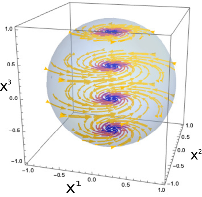
Figure 2: In these figures we have considered GKLS vector field for a 2-level atom system $\hat{H}_{\tiny\mbox{atm}}=\frac{1}{2}\,h\,\nu\,\sigma^{3}$ with a dissipative term introduced by means of the operator $\hat{v}_{1}=\sqrt{\frac{\gamma}{2}}\,\hat{\sigma}^{3}$. The GKLS vector field has been displayed in Cartesian coordinates $(x^{1},x^{2},x^{3})$, where we have considered the frequency $\nu=2$ and the damping parameter $\gamma=1$.

Let us now introduce a dissipative evolution by means of the GKLS formalism by considering the simplest case corresponding to $\hat{v}_{1}=\sqrt{\frac{\gamma}{2}}\,\hat{\sigma}^{3}$, where $\gamma$ is a constant with dimensions of frequency that modulates the dissipation, called the damping parameter. In this case, we have that $\hat{V}=\hat{v}^{\dagger}_{1}\,\hat{v}_{1}=\gamma\,\hat{\sigma}^{0}$, thus $Y_{\hat{V}}=0$; therefore, the dissipation to the Hamiltonian system is exclusively determined by the Choi–Krauss vector field.

To compute the vector field $Z_{\mathcal{K}}$ in Eq. (89), we first note that $f_{\hat{V}}=\frac{\gamma}{2}$ and $\mathcal{K}^{k}{}_{0}=0$, then

$$\frac{1}{2}\mathcal{K}^{k}{}_{j}\,x^{j}\,\frac{\partial}{\partial x^{k}}=\frac{1}{2}{\rm Tr}\{\hat{\mathcal{K}}(\sigma_{j})\,\hat{\sigma}^{k}\}x^{j}\,\frac{\partial}{\partial x^{k}}=\frac{\gamma}{4}\delta_{jl}{\rm Tr}\{\hat{\sigma}^{3}\,\hat{\sigma}^{l}\,\hat{\sigma}^{3}\,\hat{\sigma}^{k}\}x^{j}\,\frac{\partial}{\partial x^{k}}\,.$$ (97)

Taking into account the property ${\rm Tr}\{\hat{\sigma}^{i}\,\hat{\sigma}^{j}\,\hat{\sigma}^{k}\,\hat{\sigma}^{l}\}=2(\delta^{ij}\delta^{kl}-\delta^{ik}\delta^{jl}+\delta^{il}\delta^{jk})$ it is direct to show that

$$\frac{1}{2}\mathcal{K}^{k}{}_{j}\,x^{j}\,\frac{\partial}{\partial x^{k}}=\gamma\,x^{3}\frac{\partial}{\partial x^{3}}-\frac{\gamma}{2}\,x^{k}\frac{\partial}{\partial x^{k}}\,.$$ (98)

Then, the Choi–Krauss vector field in Cartesian coordinates takes the following form

$$Z_{\mathcal{K}}=-\gamma\left(x^{1}\frac{\partial}{\partial x^{1}}+x^{2}\frac{\partial}{\partial x^{2}}\right)\,.$$ (99)

Once calculated the Hamiltonian and Choi–Kraus terms, we can finally give the expression for the GKLS vector field

$$\Gamma=-(\nu\,x^{2}+\gamma\,x^{1})\frac{\partial}{\partial x^{1}}+(\nu\,x^{1}-\gamma\,x^{2})\frac{\partial}{\partial x^{2}}\,.$$ (100)

The vector field $\Gamma$ is displayed in Fig. 2, where the ball $\mathbf{B}$ is also plotted considering the Cartesian coordinates $(x^{1},x^{2},x^{3})$. We observe that the line $(0,0,x^{3})$ is singular and behaves as an attractor and then any pure state converge as a state with some statistical mix. In particular for the initial condition with $x^{3}=0$ the vector field ends to the state with maximal mix.

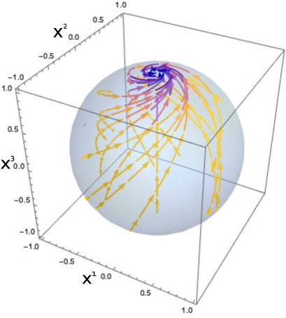
Figure 3: In this figure we plot the GKLS vector field for a 2-level atom system $\hat{H}_{\tiny\mbox{atm}}=\frac{1}{2}\,h\,\nu\,\hat{\sigma}^{3}$ with dissipative part introduced by means of the operator $\hat{v}_{1}=\sqrt{2\,\gamma}\,\hat{\sigma}_{+}$. Here we have considered the Cartesian coordinates $(x^{1},x^{2},x^{3})$ in the ball, with parameters $\nu=2$ and $\gamma=1$.

Another interesting case is to consider the transition operators to model a different dissipative dynamics. Let $v_{1}~{}=~{}\sqrt{2\,\gamma}\,\sigma_{+}$, $\hat{V}=\hat{v}^{\dagger}_{1}\,\hat{v}_{1}=\gamma\,(\hat{\sigma}^{0}-\hat{\sigma}^{3})$ and $f_{\hat{V}}=\gamma\,(1-x^{3})$. By a straightforward calculation we find that

$$-\delta^{kj}\,V_{k}\,\frac{\partial}{\partial x^{j}}=\gamma\,\frac{\partial}{\partial x^{3}}\,,\qquad-V_{0}\,\Delta=-\gamma\,x^{k}\frac{\partial}{\partial x^{k}}$$ (101)

and

$$\frac{1}{2}\mathcal{K}^{k}{}_{\mu}\,x^{\mu}\,\frac{\partial}{\partial x^{k}}=\frac{1}{2}{\rm Tr}\{\hat{\mathcal{K}}(\sigma_{0})\,\hat{\sigma}^{k}\}\,\frac{\partial}{\partial x^{k}}+\frac{1}{2}{\rm Tr}\{\hat{\mathcal{K}}(\sigma_{j})\,\hat{\sigma}^{k}\}x^{j}\,\frac{\partial}{\partial x^{k}}=\gamma\,(1-x^{3})\frac{\partial}{\partial x^{3}}\,.$$ (102)

Then, the GKLS vector field is given by

$$\Gamma=-\left(\nu\,x^{2}+\gamma\,x^{1}\right)\frac{\partial}{\partial x^{1}}+\left(\nu\,x^{1}-\gamma\,x^{2}\right)\frac{\partial}{\partial x^{2}}+2\,\gamma\,(1-x^{3})\frac{\partial}{\partial x^{3}}\,.$$ (103)

We see that the components in the $x^{1}$ and $x^{2}$ directions are the same as those of the previous case, c.f. (100); nevertheless, in the present case $\Gamma$ has a component in the $x^{3}$ direction. The integral curves corresponding to (103) are the solutions to the linear system of equations

$$\dot{x}^{1} =-\nu\,x^{2}-\gamma\,x^{1}\,,$$

$$\dot{x}^{2} =\nu\,x^{1}-\gamma\,x^{2}\,,$$

$$\dot{x}^{3} =2\,\gamma\,(1-x^{3})\,.$$ (104)

From this vector field we see that there is only one singular point in $(0,0,1)$, i.e., the “north pole” of the sphere, which is an attractor. The behaviour of this vector field is illustrated in Fig. (3). We notice that regardless of the initial condition the evolution converges to the “north pole” of the sphere.

III GKLS dynamics on Gaussian states

In this section, we are interested in obtaining the GKLS vector field for a class of systems whose quantum states are described by Gaussian states. We will follow, in general, the same steps taken for constructing the vector field for the q-bit systems and we will apply the result to describe a quantum harmonic oscillator with dissipation. Before we begin the procedure to construct the GKLS vector field, let us first review some important properties of Gaussian states.

A Gaussian state in the position space representation has the general form

$$\langle q^{\prime}|\,\hat{\rho}\,|q\rangle=\frac{1}{\sqrt{2\,\pi\,\sigma^{2}_{q}}}\exp\Bigg{\{}\frac{1}{2\,\sigma^{2}_{q}}\left[\frac{\sigma_{qp}}{\hbar}(q-q^{\prime})-\frac{{\rm i}}{2}\,(q+q^{\prime}-2\langle\hat{q}\rangle)\right]^{2}-\frac{\sigma^{2}_{p}}{2\,\hbar^{2}}(q-q^{\prime})^{2}+\frac{{\rm i}}{\hbar}\,\langle\hat{p}\rangle\,(q-q^{\prime})\Bigg{\}}\,,$$ (105)

where $q$ and $q^{\prime}$ are the coordinates in the position space for two different points. The uncertainty for each operator is defined as

$$\sigma^{2}_{q}=\langle\hat{q}^{2}\rangle-\langle\hat{q}\rangle^{2}\,\qquad\sigma^{2}_{p}=\langle\hat{p}^{2}\rangle-\langle\hat{p}\rangle^{2}\,,$$ (106)

and the correlation between the position and momentum operators is

$$\sigma_{qp}=\frac{1}{2}\langle\hat{q}\,\hat{p}+\hat{p}\,\hat{q}\rangle-\langle\hat{q}\rangle\langle\hat{p}\rangle\,.$$ (107)

For simplicity, in the following we will consider that the expectation values of position and momentum are zero, i.e. $(\langle\hat{q}\rangle,\langle\hat{p}\rangle)=(0,0)$.

A simplified expression of the Gaussian state can be obtained in the Wigner representation $W_{r}(q,p)$ of $\hat{\rho}$ by applying the Wigner-Weyl transformation Weyl-1927 to obtain the Wigner quasi-distribution function

$$W_{r}(q,p)=\frac{1}{\pi\,\hbar\,r}\exp\left\{-\frac{2}{\hbar^{2}\,r^{2}}\left[\sigma_{p}^{2}q^{2}-2\sigma_{qp}qp+\sigma_{q}^{2}p^{2}\right]\right\}\,,$$ (108)

where $(q,p)$ denote points in phase space and the parameter $r\in[1,\infty)$, related to the Robertson-Schrödringer uncertainty relation, is defined as

$$\sigma_{q}^{2}\,\sigma_{p}^{2}-\sigma^{2}_{qp}=\frac{\hbar^{2}\,r^{2}}{4}\,.$$ (109)

In addition, it can be shown by direct calculation that the degree of non-purity of a Gaussian state is given by the parameter $r$, due to

$${\rm Tr}\{\hat{\rho}^{2}\}=\frac{1}{r}\,.$$ (110)

In particular, when $r=1$ the density Gaussian matrix or the Wigner function corresponds to the generalized coherent states, see for instance Ref. Cruz-2021 ; Perelomov-1977 ; Zhang-1990 ; Cruz-2015 . Hence, in this case, the Gaussian density matrix may be factorized as $\hat{\rho}=|0\rangle\langle 0|$ where $|0\rangle$ denotes the vacuum state of the Fock states.

The normalized positive functional $\langle q^{\prime}|\,\hat{\rho}\,|q\rangle$ or equivalently its associated Wigner function $W_{r}(q,p)$ describing the quantum states is parametrized by $(\sigma_{q}^{2},\sigma_{p}^{2},\sigma_{qp})$ and these parameters are constrained by the relation (109). We are interested in defining a manifold for the entire space of states parametrized by the uncertainties and the correlation. In order to do so, we consider the immersion of a finite-dimensional manifold into the space of normalized positive functionals $\mathcal{L}^{1}$ by means of a Weyl map Ercolessi-2010 .

To introduce the Weyl map, it is important to first make some remarks of the space of parameters. To describe the immersion of the space of second momenta $(\sigma_{q}^{2},\sigma_{p}^{2},\sigma_{qp})$, one intoduces the following set of coordinates

$$y^{1}=\frac{1}{\hbar}(\sigma^{2}_{p}+\sigma^{2}_{q})\,,\qquad y^{2}=\frac{2}{\hbar}\,\sigma_{qp}\,,\qquad y^{3}=\frac{1}{\hbar}(\sigma^{2}_{p}-\sigma^{2}_{q}),$$ (111)

such that the constraint (109) defines the manifold for a fix value of $r$ as

$$h_{r}=\{(y^{1},y^{2},y^{3})\in{\mathbb{R}}^{3}\,|\,(y^{1})^{2}-(y^{2})^{2}-(y^{3})^{2}=r^{2}\}\,,$$ (112)

where $y^{1}>0$. The manifolds $h_{r}$ are consequently upper-hyperboloids in ${\mathbb{R}}^{3}$ known as pseudo-spheres, in analogy to the spheres in the q-bit case Balazs-1986 . From the expression (110), it is clear that each manifold $h_{r}$ has a different degree of statistical mixture, while the purity condition ${\rm Tr}\{\hat{\rho}^{2}\}=1$ identifies the hyperboloid

$$H^{2}=\{(y^{1},y^{2},y^{3})\in{\mathbb{R}}^{3}\,|\,(y^{1})^{2}-(y^{2})^{2}-(y^{3})^{2}=1\}\,.$$ (113)

On the other hand, the condition ${\rm Tr}\{\hat{\rho}^{2}\}<1$ identifies the non-pure states as the set defined by

$$(y^{1})^{2}-(y^{2})^{2}-(y^{3})^{2}>1\,,$$ (114)

where the maximal “impurity” is obtained for the state in the limit $r\to\infty$. Therefore, a general Gaussian state is parametrized by points $\mathbf{y}=(y^{1},y^{2},y^{3})$ in the three-dimensional differential manifold

$$\mathbf{H}=\{(y^{1},y^{2},y^{3})\in{\mathbb{R}}^{3}\,|\,(y^{1})^{2}-(y^{2})^{2}-(y^{3})^{2}\geq 1\}\,.$$ (115)

The space $\mathbf{H}$ is a differential manifold with boundary and it can be described as the foliation given by the hyperboloids (112) labeled by $r$ as

$$\mathbf{H}=\bigcup_{r\geq 1}h_{r}\,,$$ (116)

where the leaves of this foliation are defined in Eq. (112) and on each leaf a differential structure can be given. A schematic picture of this foliation is displayed in Fig. 4. The foliated space $\mathbf{H}$ can be identified with the orthochronous Lorentz group $SO(1,2)$ which acts smoothly on itself. Equivalently, one may employ the two-fold covering group $SU(1,1)$ of $SO(1,2)$ or one of its isomorphic groups $SL(2,{\mathbb{R}})$ and $Sp(2,{\mathbb{R}})$ Wolf-1986 ; Kastrup-2003 ; Balachandran-2010 .

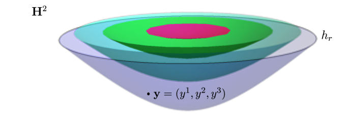
Figure 4: Pictorial representation of the space of the solid $\mathbf{H}$. A Gaussian state is represented by a point $\mathbf{y}=(y^{1},y^{2},y^{3})$ in $\mathbf{H}$. In addition, one may see that this solid is foliated by a the disjoint family of hyperboloids $h_{r}$.

There is a clear analogy between the ball $\mathbf{B}$ employed in the description of q-bit systems and the solid hyperboloid $\mathbf{H}$, in the sense that they are manifolds containing the information of the quantum states and both manifolds are foliated such that each leaf of the foliation has a fix degree of purity.

We are interested in describing the immersion of each leaf $h_{r}$ into the space of normalized positive functionals $\mathcal{L}^{1}$, then, we will require to find a set of coordinates for $h_{r}$. For instance, one may introduce hyperbolic coordinates by considering the mapping $\nu:h_{r}\to{\mathbb{C}}$, where each point $(y^{1},y^{2},y^{3})$ on $h_{r}$ is described by a point in the complex plane $\kappa_{r}=\frac{\tau}{2}\,{\rm e}^{{\rm i}\,\varphi}$ given by

$$y^{1}=r\cosh{\tau}\,,\quad y^{2}=r\sinh{\tau}\cos{\varphi}\,,\quad y^{3}=r\sinh{\tau}\sin{\varphi}\,,$$ (117)

The coordinates $(\tau,\varphi)$ are called squeezing parameters in quantum optics Scully-1999 .

Now we are in position to introduce the Weyl map from $h_{r}$ to the set of unitary operators

$$\hat{S}(\xi_{r})\equiv\exp\left[\bar{\kappa}_{r}\,\hat{K}_{-}-\kappa_{r}\,\hat{K}_{+}\right]$$ (118)

known as squeezing operators, where the operators $\hat{K}_{\pm}$ together with $\hat{K}_{0}$ are the generators of the Lie algebra ${\mathfrak{su}}(1,1)$ satisfying the commutation relations

$$[\hat{K}_{+},\hat{K}_{-}]=-2\,\hat{K}_{0}\,,\quad[\hat{K}_{0},\hat{K}_{\pm}]=\pm\,\hat{K}_{\pm}\,.$$ (119)

Therefore, we have defined the map $W:h_{r}\to\mathcal{U}({\mathcal{H}}):\kappa_{r}\mapsto\hat{S}(\kappa_{r})$, denoting $\mathcal{U}({\mathcal{H}})$ the set of unitary operators on a Hilbert space ${\mathcal{H}}$, where the unitary representation of $h_{r}$ is given by the squeezing operator $\hat{S}(\kappa_{r})$. Furthermore, the Weyl map allows to introduce the immersion

$$w:h_{r}\to\mathcal{L}^{1}\,,$$ (120)

defined in the following form, given a fiducial state $\rho_{0}\in\mathcal{L}^{1}$ we define the action of the map $w$ as

$$w:\kappa_{r}\mapsto\hat{\rho}(\kappa_{r})\equiv\hat{S}(\kappa_{r})\,\hat{\rho}_{0}\,\hat{S}^{\dagger}(\kappa_{r})\,.$$ (121)

To be more specific, let us consider as a fiducial state the Gaussian state with zero squeezing parameters $(\tau_{r},\varphi_{r})=(0,0)$, i.e., the state has zero correlation $\tilde{\sigma}_{qp}=0$, therefore, the fiducial Gaussian state in the position representation is

$$\langle q^{\prime}|\,\hat{\rho}_{0}\,|q\rangle=\frac{1}{\sqrt{2\,\pi\,\tilde{\sigma}^{2}_{q}}}\exp\Bigg{\{}-\frac{1}{8\,\tilde{\sigma}^{2}_{q}}(q+q^{\prime})^{2}-\frac{\tilde{\sigma}^{2}_{p}}{2\,\hbar^{2}}(q-q^{\prime})^{2}\Bigg{\}}\,.$$ (122)

Acting with the squeezing operator there is a translation in $h_{r}$ from $(0,0)$ to $(\tau_{r},\varphi_{r})$ which in terms of the uncertainties and the correlation is given by the map $(\tilde{\sigma}^{2}_{q},\tilde{\sigma}^{2}_{p},0)\mapsto(\sigma^{2}_{q},\sigma^{2}_{p},\sigma_{qp})$ defined by the transformation

$$\sigma^{2}_{q} =\tilde{\sigma}^{2}_{q}\left[\,\cosh{\tau_{r}}-\cos{\varphi_{r}}\,\sinh{\tau_{r}}\,\right]\,,$$

$$\sigma^{2}_{p} =\tilde{\sigma}^{2}_{p}\left[\,\cosh{\tau_{r}}+\cos{\varphi_{r}}\,\sinh{\tau_{r}}\,\right]\,,$$

$$\sigma_{qp} =-\frac{\hbar\,r}{2}\,\sin{\varphi_{r}}\,\sinh\tau_{r}\,,$$ (123)

obtaining the Gaussian density matrix

$$\langle q^{\prime}|\hat{\rho}(\kappa_{r})|q\rangle=\frac{1}{\sqrt{2\,\pi\,\sigma^{2}_{q}}}\exp\Bigg{\{}\frac{1}{2\,\sigma^{2}_{q}}\left[\frac{\sigma_{qp}}{\hbar}(q-q^{\prime})-\frac{{\rm i}}{2}\,(q+q^{\prime})\right]^{2}-\frac{\sigma^{2}_{p}}{2\,\hbar^{2}}(q-q^{\prime})^{2}\Bigg{\}}\,.$$ (124)

Let us note that because of the highly non-linearity of the squeezing parameters $(\tau_{r},\varphi_{r})$, it will result convenient to employ a set of coordinates adapted to the upper half complex plane

$$\text{HP}_{r}=\left\{{\mathcal{C}}\in{\mathbb{C}}\,|\,{\mathcal{C}}_{\tiny\mbox{I}}>0\right\}\,,$$ (125)

where ${\mathcal{C}}={\mathcal{C}}_{\tiny\mbox{R}}+{\rm i}\,{\mathcal{C}}_{\tiny\mbox{I}}$ and defined by the relations

$$y^{1}={\rm i}\,r\,\frac{1+{\mathcal{C}}\bar{{\mathcal{C}}}}{{\mathcal{C}}-\bar{{\mathcal{C}}}}\,,\qquad y^{2}={\rm i}\,r\,\frac{{\mathcal{C}}+\bar{{\mathcal{C}}}}{{\mathcal{C}}-\bar{{\mathcal{C}}}}\,,\qquad y^{3}={\rm i}\,r\frac{-1+{\mathcal{C}}\bar{{\mathcal{C}}}}{{\mathcal{C}}-\bar{{\mathcal{C}}}}\,.$$ (126)

The two-dimensional space for $r=1$ described by these coordinates is known in the literature as the Siegel upper half plane Siegel-1943 .

The infinite representations in Eqs. (105) and (108) of the Gaussian state $\hat{\rho}$ are not adequate to obtain the GKLS vector field as it was done for the q-bit case. Nevertheless, the smooth action of $SL(2,{\mathbb{R}})$ on the space of parameters $\mathbf{H}$ makes possible to define an immersion of the space of $2\times 2$ matrices into the space of parameters $(y^{1},y^{2},y^{3})$ by

$$m:\mathcal{M}_{2}\to\mathbf{H}:\hat{\xi}\mapsto(y^{1},y^{2},y^{3})\,.$$ (127)

Thus, any dynamical evolution in the space of matrices induces dynamics in the space of parameters, describing geometrically the evolution of Gaussian states. In particular, this perspective allows us to apply the same procedure as in the q-bit case to obtain the corresponding GKLS vector field. Restricting to observables quadratic in position and momentum, the set of operators ${\mathfrak{D}}$ can be identified with the subset ${\mathfrak{sl}}(2,{\mathbb{R}})$. The basis for the Lie algebra ${\mathfrak{sl}}(2,{\mathbb{R}})$ of observables $\{\hat{L}^{k}\}$ can be chosen as

$$\hat{L}^{1}=\frac{1}{4}\left(\hat{p}^{2}+\hat{q}^{2}\right)\,,\quad\hat{L}^{2}=\frac{1}{4}\left(\hat{q}\,\hat{p}+\hat{p}\,\hat{q}\right)\,,\quad\text{and}\quad\hat{L}^{3}=\frac{1}{4}\left(\hat{p}^{2}-\hat{q}^{2}\right)\,.$$ (128)

On the other hand, if ${\mathfrak{sl}}^{\ast}(2,{\mathbb{R}})$ is the dual Lie algebra, then for every $\xi\in{\mathfrak{sl}}^{\ast}(2,{\mathbb{R}})$ there is a unique $\hat{\xi}\in{\mathfrak{sl}}(2,{\mathbb{R}})$ such that

$$\langle\xi,\hat{a}\rangle:=\,{\rm Tr}\{\hat{a}\,\hat{\xi}\}\,.$$ (129)

The advantage of considering ${\mathfrak{sl}}(2,{\mathbb{R}})$ resides in that it can be given a finite matrix representation in terms of $2\times 2$ matrices

$$\hat{L}_{1}=\frac{{\rm i}\,\hbar}{2}\,\left(\begin{array}[]{c c}0&1\\ -1&0\\ \end{array}\right)\,,\quad\hat{L}_{2}=\frac{{\rm i}\,\hbar}{2}\,\left(\begin{array}[]{c c}1&0\\ 0&-1\\ \end{array}\right)\,,\quad\hat{L}_{3}=\frac{{\rm i}\,\hbar}{2}\,\left(\begin{array}[]{c c}0&1\\ 1&0\\ \end{array}\right)\,.$$ (130)

As we have seen in Section II, at some point, we will employ the Lie-Jordan algebra structure to define Hamiltonian and gradient-like dynamics for the space of parameters. Thus, it is necessary to enlarge our basis of matrices to include the element

$$\hat{L}_{0}=\frac{\hbar}{2}\,\left(\begin{array}[]{c c}1&0\\ 0&1\\ \end{array}\right)\,.$$ (131)

Then, we can define the matrix $\xi$ as

$$\xi=\frac{1}{2\,\hbar}\,y^{\mu}\,L_{\mu}\,,$$ (132)

where $\mu=0,1,2,3$, where $L_{\mu}=g_{\mu\nu}\hat{L}^{\nu}$, $y^{\mu}\equiv g^{\mu\nu}y_{\nu}$ where $g^{\mu\nu}$ are the entries of the matrix $\rm{diag}(1,1,-1,-1)$. The normalization condition ${\rm Tr}\{\hat{\xi}\}=1$ fixes $y^{0}=2$ and the components $(y^{1},y^{2},y^{3})$ can be obtained as

$$y^{k}~{}=~{}{\rm Tr}\{\hat{L}^{k}\hat{\xi}\}\,.$$ (133)

These components depend on the second moments and the correlation as can be seen from the relations (111), which can be found in this representation by

$$\sigma_{q}^{2}=\mathrm{Tr}\,\{\hat{q}^{2}\hat{\xi}\},\qquad\sigma_{p}^{2}=\mathrm{Tr}\,\{\hat{p}^{2}\hat{\xi}\}\qquad\text{and}\qquad\sigma_{qp}=\mathrm{Tr}\,\{\frac{1}{2}(\hat{q}\hat{p}+\hat{p}\hat{q})\hat{\xi}\}\,,$$ (134)

which coincide with the expectation values for the operators $\hat{q}^{2}$, $\hat{p}^{2}$ and $\frac{1}{2}(\hat{q}\hat{p}+\hat{p}\hat{q})$ obtained from the Gaussian states, as is easily verified using for instance the Wigner function to compute them. It is important to note that $\xi$ is not properly an state, because is not positive defined and its matrix representations is not self-adjoint; however, from the relation (134) one may established the map between operators and linear functions by

$$f_{\hat{a}}:=\mathrm{Tr}\{\hat{a}\,\hat{\xi}\}\,,$$ (135)

where $\hat{a}$ is an operator in ${\mathfrak{sl}}(2,{\mathbb{R}})$ and $f_{\hat{a}}$ its corresponding dual. Based on these results, we claim that the GKLS dynamics can be determined from the GKLS equation for $\xi$, making it possible to follow the procedure for finite-dimensional representations and use the Lie-Jordan algebra structure to construct the GKLS vector field on the space of parameters.

III.1 Dynamical study of Gaussian state systems from a state point of view

In quantum mechanics, under the usual probabilistic interpretation, any transformation of a state is described by a one-parameter group of unitary transformations, in particular, the time evolution of a state, i.e., the probability conservation is secured by the Schrödinger equation. The assumption of this interpretation, then requires the infinitesimal generator to be a self-adjoint operator acting on the separable complex Hilbert space ${\mathcal{H}}$ associated with the physical system. Let us describe, for the case of Gaussian states, how this unitary evolution can be cast in terms of a Hamiltonian vector field. To do so, we will make use of the Kähler structure that the upper-half-hyperboloid $h_{r}$ bears, which later will probe to be useful when we extend the dynamics adding dissipation as a perturbation term.

As we have seen in the previous subsection, the space $\mathbf{H}$ of all the quantum states described by Gaussian density matrix is foliated by leaves labeled by $r$. Each leaf $h_{r}$ is endowed with a Kähler structure $(\omega_{h_{r}},g_{h_{r}},J_{h_{r}})$, then it is possible to introduce symplectic and gradient dynamics on it by means of the definitions

$$\omega_{h_{r}}(\mathbb{X}_{H},\,\cdot\,)={\rm d}f_{\hat{H}}\,,\qquad g_{h_{r}}=(\mathbb{Y}_{H},\,\cdot\,)={\rm d}f_{\hat{H}}\,,$$ (136)

where $f_{\hat{H}}$ is a smooth functions in $h_{r}$. These functions are determined by the expectation value of a Hamiltonian operator as follows. First of all, let us restrict our study to Hamiltonian operators which are quadratic in the position and momentum operator with the general form

$$\hat{H}=\frac{1}{2}\left[H_{1}\,\hat{p}^{2}+V(\hat{q}\,\hat{p}+\hat{p}\,\hat{q})+H_{2}\,\hat{q}^{2}\right]\,,$$ (137)

where $H_{1}$, $H_{2}$ and $V$ are real constants. Therefore, the space of observables $\mathfrak{D}$ is identify with the subset of the ${\mathfrak{sl}}(2,{\mathbb{R}})$ Lie algebra consisting of self-adjoint elements. Thus, the expectation value of the Hamiltonian operator $\hat{H}$, defined as $f_{\hat{H}}:={\rm Tr}\{\hat{\rho}\,\hat{H}\}$, is given by

$$f_{\hat{H}}=\frac{1}{2}\left[H_{1}\,\langle\hat{p}^{2}\rangle+V\langle\hat{q}\,\hat{p}+\hat{p}\,\hat{q}\rangle+H_{2}\langle\hat{q}^{2}\rangle\right]\,$$ (138)

and from the definitions (106) and (107) it is not difficult to find that

$$f_{\hat{H}}=\frac{1}{2}\left[H_{1}\,\sigma^{2}_{p}+2\,V\sigma_{qp}+H_{2}\sigma_{q}^{2}\right]\,.$$ (139)

Determining the Hamiltonian and gradient dynamics boils down to obtain the vector fields $\mathbb{X}_{H}$ and $\mathbb{Y}_{H}$ as defined in (136). We can employ the coordinates adapted to the complex upper-half-plane defined in (126) for which the symplectic form and the Riemannian metric take the form

$$\omega_{h_{r}}=\frac{{\rm i}\,\hbar}{2}\frac{r^{2}}{(\bar{\mathcal{C}}-\mathcal{C})^{2}}{\rm d}\,\bar{\mathcal{C}}\wedge{\rm d}\,\mathcal{C}\qquad\text{and}\qquad g_{h_{r}}=\frac{\hbar}{2}\frac{r^{2}}{(\bar{\mathcal{C}}-\mathcal{C})^{2}}{\rm d}\,\bar{\mathcal{C}}\otimes_{\tiny\mbox{s}}{\rm d}\,\mathcal{C}\,.$$ (140)

with complex structure

$$J_{h_{r}}=\frac{1}{{\rm i}}\left({\rm d}{\mathcal{C}}\otimes\frac{\partial}{\partial{\mathcal{C}}}-{\rm d}\bar{{\mathcal{C}}}\otimes\frac{\partial}{\partial\bar{{\mathcal{C}}}}\right)\,.$$ (141)

The expectation value of the Hamiltonian operator $f_{\hat{H}}$ in (139) has the following expression in the $\mathcal{C}$ coordinate system

$$f_{\hat{H}}=\frac{{\rm i}\,\hbar}{2}\frac{r}{{\mathcal{C}}-\bar{{\mathcal{C}}}}\left[H_{1}\,{\mathcal{C}}\,\bar{{\mathcal{C}}}+V\,({\mathcal{C}}+\bar{{\mathcal{C}}})+H_{2}\right]$$ (142)

where there is a clear dependence on the parameter $r$. We may now proceed to compute the Hamiltonian and the gradient vector fields considering that they take the following generic form

$$\mathbb{X}_{H}=\mathbb{X}_{\mathcal{C}}\frac{\partial}{\partial{\mathcal{C}}}+\mathbb{X}_{\bar{{\mathcal{C}}}}\frac{\partial}{\partial\bar{{\mathcal{C}}}}\quad\text{and}\quad\mathbb{Y}_{H}=\mathbb{Y}_{\mathcal{C}}\frac{\partial}{\partial{\mathcal{C}}}+\mathbb{Y}_{\bar{{\mathcal{C}}}}\frac{\partial}{\partial\bar{{\mathcal{C}}}}\ ,$$ (143)

respectively, then employing the definition in Eq. (136) one may find that the components of these vector fields are given by

$$\mathbb{X}_{\mathcal{C}}=-\frac{2}{{\rm i}\,\hbar}\frac{({\mathcal{C}}-\bar{{\mathcal{C}}})^{2}}{r^{2}}\,\frac{\partial f_{H}}{\partial\bar{{\mathcal{C}}}}=-\frac{1}{r}\left[H_{1}\,{\mathcal{C}}^{2}+2\,V\,{\mathcal{C}}+H_{2}\right]$$ (144)

and

$$\mathbb{Y}_{\mathcal{C}}=\frac{2}{\hbar}\frac{({\mathcal{C}}-\bar{{\mathcal{C}}})^{2}}{r^{2}}\,\frac{\partial f_{H}}{\partial\bar{{\mathcal{C}}}}=\frac{{\rm i}}{r}\left[H_{1}\,{\mathcal{C}}^{2}+2\,V\,{\mathcal{C}}+H_{2}\right]\,.$$ (145)

Therefore, the symplectic evolution in these coordinates is described by the nonlinear Riccati equation

$$\dot{{\mathcal{C}}}=-\frac{1}{r}\left[H_{1}\,{\mathcal{C}}^{2}+2\,V\,{\mathcal{C}}+H_{2}\right]\,.$$ (146)

On the other hand, the equations of motion in terms of Euclidean coordinates $(y^{1},y^{2},y^{3})$ are given by the linear system of equation

$$\dot{y}^{1} =\frac{1}{r}[(H_{1}-H_{2})\,y^{2}-2\,Vy^{3}]\,,$$ (147)

$$\dot{y}^{2} =\frac{1}{r}[(H_{1}-H_{2})\,y^{3}+(H_{1}+H_{2})\,y^{1}]\,,$$ (148)

$$\dot{y}^{3} =-\frac{1}{r}[(H_{1}+H_{2})\,y^{1}+2\,Vy^{2}]\,,$$ (149)

where the solutions of this linear system of equations correspond to the integral curves of the linear system of equations obtained from the Hamiltonian vector field

$$\mathbb{X}_{H}=\frac{1}{r}(y^{2}H_{3}-y^{3}H_{2})\frac{\partial}{\partial y^{1}}+\frac{1}{r}(y^{3}H_{1}+y^{1}H_{3})\frac{\partial}{\partial y^{2}}-\frac{1}{r}(y^{1}H_{2}+y^{2}H_{1})\frac{\partial}{\partial y^{3}}\,.$$ (150)

Let us now introduce the Poisson and Jordan brackets in $h_{r}$ and establish their relation to the algebraic structures of operators in ${\mathfrak{D}}$. To this end, we start defining from $\omega_{h_{r}}$ the Poisson bracket for observables $f_{\hat{a}}$ and $f_{\hat{b}}$ associated to the operators $\hat{a}$ and $\hat{b}$, respectively. Thus, in the hyperboloid the Poisson bracket is defined by means of the symplectic form (140) defined on each leaf $h_{r}$ by

$$\{f_{\hat{a}},f_{\hat{b}}\}_{h_{r}}=\omega_{h_{r}}(\mathbb{X}_{b},\mathbb{X}_{a})\,.$$ (151)

Then, it can be shown by direct calculation that the Poisson bracket satisfies the following relation

$$\{f_{\hat{a}},f_{\hat{b}}\}_{h_{r}}=\frac{1}{r}\,f_{[[\hat{a},\hat{b}]]}\,,$$ (152)

where $[[\cdot,\cdot]]$ is the Lie-product defined in Eq. (43), where to obtain the last identity we have employed the basis $\{\hat{L}^{k}\}$ in Eq. (128) satisfying the commutation relations

$$[[\hat{L}^{1},\hat{L}^{2}]]=\hat{L}^{3}\,,\quad[[\hat{L}^{2},\hat{L}^{3}]]=-\,\hat{L}^{1}\quad\text{and}\quad[[\hat{L}^{1},\hat{L}^{3}]]=-\,\hat{L}^{2}\,.$$ (153)

On the other hand, the Jordan bracket is defined through the relation

$$\langle\langle f_{\hat{a}},f_{\hat{b}}\rangle\rangle_{h_{r}}=g_{h_{r}}(\mathbb{Y}_{a},\mathbb{Y}_{b})\,.$$ (154)

Hence, taking into account this definition, it can be shown by direct substitution that the Jordan bracket satisfies the following relation

$$\langle\langle f_{\hat{a}},f_{\hat{b}}\rangle\rangle_{h_{r}}=\frac{1}{2}\,f_{\hat{a}\odot\hat{b}}-\frac{4}{\hbar\,r^{2}}\,f_{\hat{a}}\,f_{\hat{b}}\,,$$ (155)

where $\odot$ is the Jordan-product defined in Eq. (43), which for the basis $\{\hat{L}^{k}\}$ obeys the relations

$$\hat{L}^{j}\odot\hat{L}^{k}=\frac{\hbar}{2}\,g^{jk}\,\hat{\mathbb{I}}$$ (156)

with $\hat{\mathbb{I}}$ the identity operator and $g^{jk}$ being the entries of the diagonal matrix

$$g=\left(\begin{array}[]{c c c}1&0&0\\ 0&-1&0\\ 0&0&-1\end{array}\right)\,.$$ (157)

To conclude this subsection, let us introduce a couple of bivector fields which will allow us to extend the Hamiltonian and gradient dynamics to the whole space $\mathbf{H}$. These two tensor fields will be relevant in introducing the GKLS dynamics in the following subsections. On the one hand, the skew-symmetric bivector field will permit to describe the Hamiltonian dynamics on $\mathbf{H}$ where a symplectic form cannot be defined; in this sense, this is a more general geometric field which can be used to define a Poisson bracket. On the other hand, the symmetric bivector field will serve for generalizing the gradient dynamics, although some redefinitions will be necessary to establish properly the GKLS dynamics.

The skew-symmetric bivector field in the ${\mathcal{C}}$ coordinates is given by the expression

$$\Lambda_{h_{r}}=\frac{2\,{\rm i}}{\hbar}\frac{({\mathcal{C}}-\bar{{\mathcal{C}}})^{2}}{r^{2}}\frac{\partial}{\partial\bar{{\mathcal{C}}}}\wedge\frac{\partial}{\partial{\mathcal{C}}}$$ (158)

and is such that the Poisson brackets can be defined as

$$\{f_{\hat{a}},f_{\hat{b}}\}_{h_{r}}:=\Lambda_{h_{r}}({\rm d}f_{\hat{a}},{\rm d}f_{\hat{b}})\,,$$ (159)

while the symmetric bivector field takes the form

$$G_{h_{r}}=\frac{2}{\hbar}\frac{({\mathcal{C}}-\bar{{\mathcal{C}}})^{2}}{r^{2}}\frac{\partial}{\partial\bar{{\mathcal{C}}}}\otimes_{\tiny\mbox{s}}\frac{\partial}{\partial{\mathcal{C}}}\,,$$ (160)

and the Jordan bracket is defined by the following relation

$$\langle\langle f_{\hat{a}},f_{\hat{b}}\rangle\rangle_{h_{r}}:=G_{h_{r}}({\rm d}f_{\hat{a}},{\rm d}f_{\hat{b}})\,.$$ (161)

Therefore, from the state point of view we have established the symplectic evolution and the gradient vector field which are tangent to the manifolds $h_{r}$; however, to introduce the GKLS evolution it is necessary generalize these definitions to all the manifold $\mathbf{H}$. To achieve this it is necessary to consider the observable point of view as we will see in the next section.

III.2 Dynamical study of Gaussian state systems from an observable point of view

In the previous subsections, as well as in the q-bit case, we have seen that the symplectic and gradient dynamics generated by the corresponding vector fields preserve the degree of purity on each leaf $h_{r}$, that is, the parameter $r$ remains unchanged during this type of evolution. This means non-pure states with initial conditions described by a density matrix fulfilling (110) preserve such a constraint under this dynamics. However, we aim to find a dynamical evolution for the states that does not preserve the degree of purity of the Gaussian state; in a geometric language we are looking for dynamics described by a vector field transverse to the leaves of constant $r$, that is, to the hiperboloids $\{h_{r}\}$. This evolution will take place in the manifold $\mathbf{H}$ and the change in the parameter $r$ will reflect the fact that the purity of states is changing in time.

Then, similarly to what has been done in the q-bit case, we shall establish the dynamics generated by the GKLS equation in geometrical terms, finding an affine vector field $\Gamma$ which accepts a decomposition in terms of a Hamiltonian dynamics, a gradient-like vector field and a Choi–Kraus vector field, as is expressed in Eq. (48). Thus, to do so, we will extend the definition of Hamiltonian vector field and introduce the gradient-like vector field considering a description in terms of the observables employing the Lie–Jordan structure $({\mathfrak{D}},\odot,[[\cdot,\cdot]])$ of the space of self-adjoint operators.

From the observables point of view, there is a one-to-one correspondence between each operator $\hat{a}\in{\mathfrak{D}}\subset{\mathfrak{sl}}(2,{\mathbb{R}})$ and a function $\tilde{f}_{\hat{a}}:={\rm Tr}\{\hat{a}\,\hat{\rho}\}$ in the dual space ${\mathfrak{D}}^{\ast}$; therefore, the space of functions in ${\mathfrak{D}}^{\ast}$ provides a realization of the Lie–Jordan algebra given in Eq. (50).

We may introduce a skew-symmetric and a symmetric $(2,0)$ tensor fields on ${\mathfrak{D}}^{\ast}$ by means of its Lie and Jordan algebraic structures, respectively. At each point of ${\mathfrak{D}}^{\ast}$ we have a cotangent space whose elements are the 1-forms ${\rm d}\tilde{f}_{\hat{a}}$ from the linear functions on ${\mathfrak{D}}^{\ast}$ associated to any operator $\hat{a}\in{\mathfrak{D}}$; then, we can define these bi-vector fields as

$$\tilde{\Lambda}({\rm d}\tilde{f}_{\hat{a}},{\rm d}\tilde{f}_{\hat{b}}):=\tilde{f}_{[[\hat{a},\hat{b}]]}\qquad\text{and}\qquad\tilde{G}({\rm d}\tilde{f}_{\hat{a}},{\rm d}\tilde{f}_{\hat{b}}):=\,\tilde{f}_{\hat{a}\odot\hat{b}}\,,$$ (162)

where $\tilde{f}_{\hat{a}}$ and $\tilde{f}_{\hat{b}}$ are functions in ${\mathfrak{D}}^{\ast}$. These tensor fields allow us to define a Hamiltonian vector field $\tilde{X}_{H}$ and a gradient-like vector field $\tilde{Y}_{b}$ on ${\mathfrak{D}}^{\ast}$ as follows

$$\tilde{X}_{H}=\tilde{\Lambda}({\rm d}\tilde{f}_{\hat{H}},\,\cdot\,)\qquad\text{and}\qquad\tilde{Y}_{b}=\tilde{G}({\rm d}\tilde{f}_{\hat{b}},\,\cdot\,)\,,$$ (163)

where $\tilde{X}_{H}$ and $\tilde{Y}_{b}$ are associated to the operators $\hat{H}$ and $\hat{b}$, respectively. Therefore, we obtain a Hamiltonian vector field associated to the Lie structure and a gradient like-vector field associated to the Jordan algebra structure. This Hamiltonian vector field is the infinitesimal coadjoint action of the Lie group $SL(2,{\mathbb{R}})$ on the Lie algebra, i.e. the solutions to the equations of motion are the coadjoint orbits of $SL(2,{\mathbb{R}})$.

To describe the Lie–Jordan algebraic structure a fourth element has to be added to the generators of the Lie algebra; thus, a basis of the Lie–Jordan algebra is given by $\{\hat{L}^{\mu}\}$ where $\hat{L}^{0}=\frac{\hbar}{2}\hat{\mathbb{I}}$ with $\hat{\mathbb{I}}$ is the identity element of the algebra and $\{\hat{L}^{k}\}$ are the operators defined in Eq. (128). The Lie bracket of the set of generators defines the Lie algebra through the specification of its structure constants, then, for this basis the Lie product is such that

$$[[\hat{L}^{\mu},\hat{L}^{\nu}]]=c^{\mu\nu}_{\sigma}\,\hat{L}^{\sigma}\quad\text{where}\quad c_{\sigma}^{\mu\nu}=\begin{cases}0&\text{for}\quad c_{\sigma}^{0\nu},\,\,c_{\sigma}^{\mu 0},\,\,c_{0}^{\mu\nu}\\ \\ c^{kj}_{l}&\text{given by Eq.}\,\,\eqref{sl-Lie-product}\,,\end{cases}$$ (164)

where $k$, $j$ and $l$ denotes the values $1,2,3$ of $\mu$, $\nu$ and $\sigma$, respectively, and likewise the Jordan product must fulfil

$$\hat{L}^{\mu}\odot\hat{L}^{\nu}=d_{\sigma}^{\mu\nu}\hat{L}^{\sigma}\quad\text{with}\quad d_{\sigma}^{\mu\nu}=\begin{cases}0&\text{for}\quad d_{l}^{00}\quad\text{and}\quad d_{l}^{kj}\,,\\ \\ g^{\mu\nu}&\text{for}\quad d_{0}^{\mu\nu}\,,\\ \\ \delta^{\mu}_{\sigma}&\text{for}\quad d_{\sigma}^{\mu 0}=d_{\sigma}^{0\mu}\,,\end{cases}$$ (165)

and $g^{\mu\nu}$ are the componentes of the matrix

$$g=\left(\begin{array}[]{c c c c}1&0&0&0\\ 0&1&0&0\\ 0&0&-1&0\\ 0&0&0&-1\end{array}\right)\,.$$ (166)

We want to define vector fields on ${\mathfrak{D}}^{\ast}$ to describe the dynamical evolution of systems, then, it is convenient to introduce Cartesian coordinates on ${\mathfrak{D}}^{\ast}$ associated to the basis $\{\hat{L}^{\mu}\}$ of ${\mathfrak{D}}$ by

$$f_{\hat{L}^{\mu}}={\rm Tr}\{\hat{L}^{\mu}\hat{\rho}\}=\frac{\hbar}{4}y^{\mu}\,.$$ (167)

where $\{y^{k}\}_{k=1,2,3}$ are directly connected to the second moment by the identities in (111). Hence, given the cartesian coordinate system $\{\frac{\hbar}{4}y^{\mu}\}$ we proceed to compute the coordinate expression of the tensor fields $\tilde{\Lambda}$ and $\tilde{G}$ by means of the definition (162) obtaining

$$\tilde{\Lambda}=\frac{4}{\hbar}\,c_{\sigma}^{\mu\nu}y^{\sigma}\frac{\partial}{\partial y^{\mu}}\wedge\frac{\partial}{\partial y^{\nu}}\qquad\text{and}\qquad\tilde{G}=\frac{4}{\hbar}\,d_{\sigma}^{\mu\nu}y^{\sigma}\frac{\partial}{\partial y^{\mu}}\otimes\frac{\partial}{\partial y^{\nu}}\,.$$ (168)

Given the Hamiltonian operator $\hat{H}=H_{\mu}\hat{L}^{\mu}$ and an arbitrary operator $\hat{b}=b_{\mu}\hat{L}^{\mu}$ their duals (expectation values) correspond to $\tilde{f}_{\hat{H}}=\frac{\hbar}{4}\,H_{\mu}y^{\mu}$ and $\tilde{f}_{\hat{b}}=\frac{\hbar}{4}\,b_{\mu}y^{\mu}$; then, the Hamiltonian and the gradient-like vector fields are

$$\tilde{X}_{H}=c_{\sigma}^{\mu\nu}H_{\mu}y^{\sigma}\frac{\partial}{\partial y^{\nu}}\qquad\text{and}\qquad\tilde{Y}_{b}=d_{\sigma}^{\mu\nu}b_{\mu}y^{\sigma}\frac{\partial}{\partial y^{\nu}}\,,$$ (169)

respectively.

The orbits obtained from the Hamiltonian and gradient-like vector fields must lie entirely on the space of quantum states $\mathbf{H}$ defined by the constraint $\rho(\hat{\mathbb{I}})={\rm Tr}\{\hat{\rho}\,\mathbb{I}\}=1$, that is, $\rho$ fulfills the definition of physical state. The space of quantum states is a convex subset of a closed affine subspace ${\mathfrak{T}}$ of ${\mathfrak{D}}^{\ast}$, then, in the case of systems described by a Gaussian density matrix, the dynamical trajectories that follow the quantum states are constrained to satisfy the Robertson–Schrödinger uncertainty relation

$$\sigma_{q}^{2}\,\sigma_{p}^{2}-\sigma^{2}_{qp}\geq\frac{\hbar^{2}}{4}\,.$$ (170)

Therefore, the affine subspace of quantum states is the subset of ${\mathfrak{D}}^{\ast}$ defined as

$${\mathfrak{T}}:=\{\tilde{f}_{\hat{a}}=a_{\mu}f_{\hat{L}^{\mu}}\in\mathcal{F}({\mathfrak{D}}^{\ast})\,|\,g^{kj}\tilde{f}_{{\hat{L}}^{k}}\tilde{f}_{{\hat{L}}^{j}}\geq\frac{1}{4}\,(\tilde{f}_{{\hat{L}}^{0}})^{2}\}\,,$$ (171)

which in terms of the coordinate system $\{\frac{\hbar}{4}y^{\mu}\}$ can be characterized by those points in ${\mathfrak{D}}^{\ast}$ such that $y^{0}=2$. Then, it is possible to introduce the canonical immersion $i:={\mathfrak{T}}\to{\mathfrak{D}}^{\ast}$, such that $f_{\hat{a}}=\frac{\hbar}{2}a_{0}+\frac{\hbar}{4}a_{k}y^{k}$ is the pullback of the linear function $\tilde{f}_{\hat{a}}=\frac{\hbar}{4}a_{\mu}y^{\mu}$, i.e., $f_{\hat{a}}=i^{*}\tilde{f}_{\hat{a}}$.

Consequently, we can define symmetric and skew-symmetric tensor fields $\Lambda$ and $G$ on ${\mathfrak{T}}$ by performing a reduction of the algebraic structures given in (162). Following a similar procedure as in the q-bit case, the space of functions $\mathcal{F}({\mathfrak{T}})$ can be described as the quotient space $\mathcal{F}({\mathfrak{D}}^{\ast})/\mathcal{I}$ where $\mathcal{I}\subset\mathcal{F}({\mathfrak{D}}^{\ast})$ is the closed linear subspace of functions vanishing on ${\mathfrak{T}}$. Now, in order to have an algebraic structure on $\mathcal{F}({\mathfrak{D}}^{\ast})/\mathcal{I}$ the subspace $\mathcal{I}$ must be an ideal of $\mathcal{F}({\mathfrak{D}}^{\ast})$. One may prove directly that for an element $\tilde{f}_{\hat{a}}$ in ${\mathfrak{D}}^{\ast}$ and an element $\tilde{f}_{\hat{b}}=\left(1-\frac{y^{0}}{2}\right)b_{k}y^{k}$ in $\mathcal{I}$ we have that

$$\tilde{\Lambda}({\rm d}\tilde{f}_{\hat{a}},{\rm d}\tilde{f}_{\hat{b}})=\frac{\hbar}{4}\left(1-\frac{y^{0}}{2}\right)\,c^{kl}_{m}\,y^{m}(a_{k}b_{l}-b_{k}a_{l})\,,$$ (172)

which vanishes in ${\mathfrak{T}}$, meaning that the Poisson product of $\tilde{f}_{\hat{a}}$ and $\tilde{f}_{\hat{b}}$ defined through $\tilde{\Lambda}$ is an ideal of $\mathcal{F}({\mathfrak{D}}^{\ast})$. Thus, because the differentials of the coordinate functions $\{\frac{\hbar}{4}y^{k}\}$ form a coordinate basis for the cotangent space at each point of ${\mathfrak{T}}$, then, by means of the immersion $i$ we define the Poisson bivector field on ${\mathfrak{T}}$ as

$$\Lambda({\rm d}f_{\hat{L}^{k}},{\rm d}f_{\hat{L}^{j}}):=f_{[[\hat{L}^{k},\hat{L}^{j}]]}=c^{kj}_{l}f_{\hat{L}^{l}}\,,$$ (173)

or equivalently

$$\Lambda({\rm d}y^{k},{\rm d}y^{j})=\frac{4}{\hbar}\,c^{kj}_{l}y^{l}\,,$$ (174)

hence, $\Lambda$ has the explicit form

$$\Lambda:=\frac{4}{\hbar}\,c^{kj}_{l}y^{l}\frac{\partial}{\partial y^{k}}\wedge\frac{\partial}{\partial y^{j}}=-\frac{4}{\hbar}\left(y^{1}\,\frac{\partial}{\partial y^{2}}\wedge\frac{\partial}{\partial y^{3}}+y^{2}\,\frac{\partial}{\partial y^{1}}\wedge\frac{\partial}{\partial y^{3}}-y^{3}\,\frac{\partial}{\partial y^{1}}\wedge\frac{\partial}{\partial y^{2}}\right)\;.$$ (175)

Given the reduced bivector field $\Lambda$ on ${\mathfrak{T}}$ we define the Hamiltonian vector field $X_{\hat{H}}:=\Lambda({\rm d}f_{\hat{H}},\,\cdot\,)$, whose coordinate expression can be obtained considering the linear function $i^{*}\tilde{f}_{\hat{H}}=f_{\hat{H}}=\frac{\hbar}{2}H_{0}+\frac{\hbar}{4}\,H_{k}\,y^{k}$ associated to the Hamiltonian operator, this is,

$$X_{H}=c^{kj}_{l}H_{k}\,y^{l}\frac{\partial}{\partial y^{j}}=-(y^{3}H_{2}-y^{2}H_{3})\frac{\partial}{\partial y^{1}}+(y^{1}H_{3}+y^{3}H_{1})\frac{\partial}{\partial y^{2}}-(y^{1}H_{2}+y^{2}H_{1})\frac{\partial}{\partial y^{3}}\,.$$ (176)

An additional advantage of deducing the dynamics from an observable (algebraic) point of view is that a constant of motion can be obtained from the Casimir operator, which in this case is $\hat{C}=(\hat{L}^{1})^{2}-(\hat{L}^{2})^{2}-(\hat{L}^{3})^{2}$, and whose expectation value gives the constant of motion

$$f_{\hat{C}}=(f_{L^{1}})^{2}-(f_{L^{2}})^{2}-(f_{L^{3}})^{2}=\frac{\hbar^{2}}{4^{2}}[(y^{1})^{2}-(y^{2})^{2}-(y^{3})^{2}]\,.$$ (177)

This constant of motion allows to easily verify that $\Lambda({\rm d}\,f_{H},{\rm d}\,f_{C})=0$, therefore, the Hamiltonian vector field $X_{\hat{H}}$ is tangent to the manifolds $\{h_{r}\}$. Moreover, from this result it can be seen that the affine space is actually the manifold $\mathbf{H}$ defined in Eq. (115).

In what refers to the gradient vector field $\tilde{Y}_{\hat{b}}=\tilde{G}({\rm d}\tilde{f}_{\hat{b}},\cdot\,)$, it is not difficult to show that $\tilde{Y}_{\hat{b}}(f_{\hat{C}})\neq 0$; then, it can be shown that upon reduction of $\tilde{Y}_{\hat{b}}$ we will obtain a vector field $Y_{\hat{b}}$ that generates a dynamical evolution that is not necessarily restricted to the manifold $\mathbf{H}$; in particular, we are interested in vector fields that are tangent to the space of pure states. To amend this situation, we proceed to perform a reduction procedure for the symmetrical bivector $\tilde{G}$; however, it is not difficult to show that $\mathcal{I}$ is not an ideal of $\mathcal{F}({\mathfrak{D}}^{\ast})$ under this product because of

$$\tilde{G}({\rm d}\tilde{f}_{\hat{a}},{\rm d}\tilde{f}_{\hat{b}})=\frac{\hbar}{4}\left(1-\frac{y^{0}}{2}\right)(y^{0}g^{kl}\,a_{k}b_{l}+a_{0}\,b_{k}x^{k})-\frac{\hbar}{8}\,a_{0}y^{0}\,b_{k}y^{k}-\frac{\hbar}{8}\,a_{k}y^{k}\,b_{n}y^{n}\,.$$ (178)

for $\tilde{f}_{\hat{b}}\in\mathcal{I}$ and an arbitrary $\tilde{f}_{\hat{a}}\in\mathcal{F}({\mathfrak{D}}^{\ast})$. Then, it is necessary to modify this symmetrical bivector. Following the procedure for the q-bit case and taking into account the result in (155) one may start modifying the bivector by $\tilde{G}-\frac{4}{\hbar}\tilde{\Delta}\otimes\tilde{\Delta}$ with $\tilde{\Delta}=y^{\mu}\frac{\partial}{\partial y^{\mu}}$; however, it takes a straightforward calculation to show that on the affine space

$$\tilde{G}({\rm d}\tilde{f}_{\hat{a}},{\rm d}\tilde{f}_{\hat{b}})-\frac{4}{\hbar}\tilde{\Delta}({\rm d}\tilde{f}_{\hat{a}})\tilde{\Delta}({\rm d}\tilde{f}_{\hat{b}})\neq 0,$$ (179)

hence, its associated algebraic product is not in the subset $\mathcal{I}$. Furthermore, it can be shown that there is not a linear combination of the tensor fields $\tilde{G}$ and $\tilde{\Delta}\otimes\tilde{\Delta}$ which defines a product such that $\mathcal{I}$ is an ideal. Then, it is necessary to find a fine-tuned definition for a tensor field that allows to properly accomplish the reduction process. A possibility is to slightly modify the $\tilde{G}$ and introduce a different vector field $\tilde{\Delta}$ to define the following tensor field

$$\tilde{\mathcal{R}}:=\frac{1}{2}\,\mathcal{G}-\frac{4}{\hbar}\,\tilde{\Delta}\otimes\tilde{\Delta}\,,$$ (180)

where now $\tilde{\Delta}=\frac{y^{0}}{4}\frac{\partial}{\partial y^{0}}+y^{k}\frac{\partial}{\partial y^{k}}$ and

$$\mathcal{G}=\frac{4}{\hbar}\,\tilde{d}^{\mu\nu}_{\sigma}\,y^{\sigma}\,\frac{\partial}{\partial y^{\mu}}\otimes\frac{\partial}{\partial y^{\nu}}\,,$$ (181)

with $\tilde{d}^{00}_{0}=d^{00}_{0}-\frac{3}{2y^{0}}$ and all the other constants in (165) remaining the same, i.e., $\tilde{d}^{\mu k}_{0}=d^{\mu k}_{0}$ and $\tilde{d}^{\mu\nu}_{k}=d^{\mu\nu}_{k}$. Notice that the vector field $\tilde{\Delta}$ is a modification of the Euler-Liouville vector field. This tensor field allows us to define a product for the space of functions $\mathcal{F}({\mathfrak{D}}^{\ast})$ for which $\mathcal{I}$ is an ideal with respect to it, in fact it is direct to check that

$$\tilde{\mathcal{R}}({\rm d}\tilde{f}_{\hat{a}},{\rm d}\tilde{f}_{\hat{b}})=\left(1-\frac{y^{0}}{2}\right)\left(\frac{\hbar}{8}y^{0}g^{kl}\,a_{k}b_{l}+\frac{\hbar}{8}a_{0}\,b_{k}x^{k}(1-y^{0})-\frac{5\hbar}{16}\,a_{k}y^{k}\,b_{n}x^{n}\right)+\frac{3\hbar}{32}\,b_{k}y^{k}\,\left(1-\frac{(y^{0})^{2}}{4}\right)\,,$$ (182)

which is an element of the ideal. In particular, it will prove useful to have the tensor field $\tilde{\mathcal{R}}$ expressed in terms of the bivector field $\tilde{G}$ introduced in (168) by

$$\tilde{\mathcal{R}}=\frac{1}{2}\tilde{G}-\frac{3}{\hbar}\,\frac{\partial}{\partial y^{0}}\otimes\frac{\partial}{\partial y^{0}}-\frac{4}{\hbar}\tilde{\Delta}\otimes\tilde{\Delta}\,.$$ (183)

In this manner, the gradient-like vector field associated to $\tilde{f}_{\hat{b}}=\frac{\hbar}{4}b_{\mu}y^{\mu}$ is

$$\tilde{\mathcal{R}}({\rm d}{\tilde{f}}_{\hat{b}}\,,\,\cdot\,)=\frac{1}{2}\tilde{Y}_{\hat{b}}-\frac{3}{4}b_{0}\frac{\partial}{\partial y^{0}}-\left(b_{0}\frac{y^{0}}{4}+b_{k}y^{k}\right)\tilde{\Delta}\,.$$ (184)

where the gradient-like vector field $\tilde{Y}_{\hat{b}}$ is defined in (163).

Once we have defined the symmetrical product $\tilde{\mathcal{R}}$, we may proceed to perform the reduction by means of the immersion $i^{*}\tilde{f}_{\hat{H}}=f_{\hat{H}}=\frac{\hbar}{2}H_{0}+\frac{\hbar}{4}\,H_{k}\,y^{k}$, to obtain the reduced symmetric bivector $\mathcal{R}$ defined by

$$\mathcal{R}({\rm d}f_{\hat{L}^{k}}.{\rm d}f_{\hat{L}^{j}})=\frac{1}{2}f_{\hat{L}^{k}\odot\hat{L}^{j}}-\frac{4}{\hbar}\,f_{\hat{L}^{k}}\,f_{\hat{L}^{j}}\,,$$ (185)

such that in Cartesian coordinates takes the form

$$\mathcal{R}=\frac{4}{\hbar}\left(g^{kj}-y^{k}y^{j}\right)\frac{\partial}{\partial y^{k}}\otimes\frac{\partial}{\partial y^{j}}\,,$$ (186)

where we have denoted $\Delta=y^{k}\frac{\partial}{\partial y^{k}}$. Now, by means of $\mathcal{R}$ we can define the gradient-like vector field associated to the linear function $f_{\hat{b}}=\frac{\hbar}{2}b_{0}+\frac{\hbar}{4}b_{k}y^{k}$, which results in

$$Y_{b}:=\mathcal{R}({\rm d}f_{\hat{b}},\,\cdot\,)=\left(g^{kj}-y^{k}y^{j}\right)b_{k}\,\frac{\partial}{\partial y^{j}}\,,$$ (187)

where it is important to note that the last term in this gradient-like vector field is a quadratic term with respect to the Cartesian coordinate system.

To finalize this subsection, we want to verify that the gradient-like vector field $Y_{b}$ generates a dynamic evolution that is transverse to the leaves $h_{r}$ but tangent to $H^{2}$ when $r=1$, that is, when the initial conditions are those of a pure state; this means that the states reached from a dynamic evolution dictated by $Y_{b}$, regardless of the initial conditions, are contained within $\mathbf{H}$. To do so, we compute the Lie derivative of $f_{\hat{C}}$ along the direction of the gradient-like vector field $Y_{b}$ obtaining

$$\pounds_{Y_{b}}\,f_{\hat{C}}=\frac{\hbar^{2}}{2}\left(1-r^{2}\right)b_{k}y^{k}\,.$$ (188)

Thus, we observe that the Lie derivative is different from zero if and only if $r\neq 1$; therefore, the gradient-like vector field $Y_{b}$ is transversal to the leaves $h_{r}$ and is tangent to the hyperboloid $H^{2}$. Moreover, when $r=1$, the gradient-like vector field $Y_{b}$ is identical to the gradient vector field $\mathbb{Y}_{b}$, meaning that dynamics generated by $Y_{b}$ does not change the purity of the states, because a pure state remains pure under its evolution.

III.3 GKLS dynamics for Gaussian states

In this subsection we construct a geometric description of the GKLS dynamics of physical systems described by a Gaussian states. This is done introducing a vector field which is defined from the GKLS master equation; this vector field is transverse to the foliation $\{h_{r}\}$ and can describe the evolution of a pure state into a non-pure one. To introduce the GKLS vector field we will follow the same procedure as for the q-bit system in the previous section, thus, to achieve that, it convenient to consider the immersion of the space of $(2\times 2)$-matrices into the space of parameters $(y^{1},y^{2},y^{3})$ established in Eq. (127). Let $\hat{\xi}\in sl(2,{\mathbb{R}})$ be an operator defined as

$$\hat{\xi}=\frac{1}{2\hbar}y_{\mu}\hat{L}^{\mu}\,,$$ (189)

where the coefficients $\{y_{\mu}\}$ are related to a set of coordinate functions on the dual space. Then, the map between operators and linear functions is given by the following definition: let $\hat{T}$ be an operator in $sl(2,{\mathbb{R}})$ and $\tilde{f}_{\hat{T}}$ its corresponding dual, then the relation between them is given by

$$\tilde{f}_{\hat{T}}:=\mathrm{Tr}\{\hat{T}\,\hat{\xi}\}\,.$$ (190)

This relation can also be defined as the natural pairing between elements of the algebra and its dual

$$\xi(\hat{T}):=\langle\xi,\hat{T}\rangle={\rm Tr}\{\hat{T}\,\hat{\xi}\}\,,$$ (191)

where $\xi\in sl^{\ast}(2,{\mathbb{R}})$ is the corresponding dual to $\hat{\xi}$ given by

$$\xi=\frac{1}{2\hbar}\,y^{\mu}\,L_{\mu}\,,$$ (192)

where $L_{\mu}\equiv g_{\mu\nu}\hat{L}^{\nu}$, $y^{\mu}\equiv g^{\mu\nu}y_{\nu}$ and $g_{\mu\nu}$ are the components of the matrix (166). Thus, in terms of its matrix representation, $\xi$ takes the following form

$$\xi=\frac{1}{2\hbar}\,y^{\mu}\,L_{\mu}=\frac{{\rm i}}{2\hbar}\,\left(\begin{array}[]{c c}-\sigma_{qp}-{\rm i}\,\hbar&\sigma_{q}^{2}\\ -\sigma_{p}^{2}&\sigma_{qp}-{\rm i}\,\hbar\\ \end{array}\right)\,.$$ (193)

Then, we can define a coordinate system $\{\frac{\hbar}{4}y^{\mu}\}$ for the dual space ${\mathfrak{sl}}^{\ast}(2,{\mathbb{R}})$ related to the generators $\{\hat{L}^{\mu}\}$ of the Lie-Jordan algebra through the map (190)

$$f_{\hat{L}^{\mu}}=\langle\xi,\hat{L}^{\mu}\rangle={\rm Tr}\{\hat{L}^{\mu}\,\hat{\xi}\}=\frac{\hbar}{4}y^{\mu}\,.$$ (194)

Consequently, we have that the expectation value of an arbitrary operator $\hat{a}=a_{\mu}\,\hat{L}^{\mu}\in{\mathfrak{D}}$ corresponds to $\tilde{f}_{\hat{a}}=\langle\xi,\hat{a}\rangle=\frac{\hbar}{4}a_{\mu}y^{\mu}$.

Therefore, although $\hat{\xi}$ is not a density matrix, through the constraint $\mathrm{det}\{\frac{1}{{\rm i}}(\hat{\xi}-\hat{L}^{0})\}\geq 0$ we can state the condition for having physical states and we are able to establish a one-to-one connection between operators and their expectation values which is equivalent, in the sense that it reproduces the same mapping between ${\mathfrak{D}}$ and ${\mathfrak{D}}^{\ast}$, as the density matrix would do. The reason to proceed in this manner is that using $\hat{\xi}$ instead of $\hat{\rho}$ has the advantage of a great simplification in the calculations. Then, once established a map between ${\mathfrak{D}}$ and ${\mathfrak{D}}^{\ast}$ using the matrix representation of the Jordan–Lie algebra, we may now introduce the GKLS generator $\mathbf{L}$ acting on $\hat{\xi}$

$$\mathbf{L}(\hat{\xi})=-\frac{{\rm i}}{\hbar}[\hat{H},\hat{\xi}]_{-}-\frac{1}{2}\sum^{3}_{j}[\hat{v}_{j}^{\dagger}\,\hat{v}_{j},\hat{\xi}]_{+}+\sum^{3}_{A}\hat{v}_{j}\,\hat{\xi}\,\hat{v}_{j}^{\dagger}\,,$$ (195)

where $\hat{H}\in{\mathfrak{D}}$ is the Hamiltonian operator and $\hat{v}_{A}$ an arbitrary element of ${\mathfrak{sl}}(2,{\mathbb{R}})$. This generator can be expressed in terms of the Lie and the Jordan products

$$\mathbf{L}(\hat{\xi})=-[[\hat{H},\hat{\xi}]]-\frac{\hbar}{2}\,\hat{V}\odot\hat{\xi}+\hat{\mathcal{K}}(\hat{\xi})\,,$$ (196)

where

$$\hat{V}=\sum_{j}\hat{v}_{j}^{\dagger}\hat{v}_{j}$$ (197)

and the completely positive map is

$$\hat{\mathcal{K}}(\hat{\xi})=\sum_{j}\hat{v}_{j}\,\hat{\xi}\,\hat{v}_{j}^{\dagger}\,.$$ (198)

Let us now, in analogy with the analysis performed for the q-bit system, propose that the vector field on ${\mathfrak{D}}^{\ast}$ associated with the $\mathbf{L}$ generator takes the form

$$\tilde{\Gamma}=\tilde{X}_{H}-\frac{\hbar}{2}\,\tilde{Y}_{V}+\tilde{Z}_{\mathcal{K}}\,,$$ (199)

where $\tilde{X}_{H}$ is the Hamiltonian vector field $\tilde{\Lambda}(d\tilde{f}_{\hat{H}},\cdot\ )=\tilde{X}_{H}$, $\tilde{Y}_{V}$ is the gradient-like vector field $\tilde{G}({\rm d}\tilde{f}_{\hat{V}},\cdot\ )=\tilde{Y}_{V}$ and $\tilde{Z}_{\mathcal{K}}$ is the vector field associated with the completely positive map $\hat{\mathcal{K}}$.

To find the explicit form of the GKLS vector field we consider the master equation for $\hat{\xi}$ in terms of the Lie and Jordan products and the complete positive map (196); expressing the Hamiltonian operator as $\hat{H}=H_{\mu}\,\hat{L}^{\mu}$ the Lie product of $\hat{H}$ and $\hat{\xi}$ is

$$[[\hat{H},\hat{\xi}]]=c_{\sigma}^{\mu\nu}H_{\mu}\,y_{\nu}\,\hat{L}^{\sigma}\,,$$ (200)

while the Jordan product of $\hat{V}=V_{\mu}\hat{L}^{\mu}$ and $\hat{\xi}$ is expressed as

$$\hat{V}\odot\hat{\xi}=d^{\mu\nu}_{\sigma}V_{\mu}y_{\nu}\hat{L}^{\sigma}\,.$$ (201)

Finally, we compute explicitly the completely positive map $\mathcal{K}(\hat{\xi})$ in terms of the generators of ${\mathfrak{sl}}(2,{\mathbb{R}})$. Expressing it as

$$\hat{\mathcal{K}}(\hat{\xi})=\frac{4}{\hbar}\,\mathcal{K}_{\mu}\,\hat{L}^{\mu}=\frac{4}{\hbar}\,\left\langle L_{\mu}\,,\,\hat{\mathcal{K}}(\hat{\xi})\right\rangle\,\hat{L}^{\mu}\,,$$ (202)

where the coefficients $\mathcal{K}_{\mu}$ are given by

$$\mathcal{K}_{\mu}=\left\langle L_{\mu}\,,\,\hat{\mathcal{K}}(\hat{\xi})\right\rangle=\frac{1}{2\hbar}{\rm Tr}\left\{\sum_{A}\hat{v}_{A}\hat{L}^{\nu}\hat{v}_{A}^{\dagger}\hat{L}^{\alpha}\right\}y_{\nu}g_{\alpha\mu}\,,$$ (203)

which can also be expressed as $\mathcal{K}_{\mu}=\mathcal{K}^{\nu}{}_{\mu}\,y_{\nu}$ where

$$\mathcal{K}^{\nu}{}_{\mu}=\frac{1}{2\hbar}{\rm Tr}\left\{\sum_{A}\hat{v}_{A}\hat{L}^{\nu}\hat{v}_{A}^{\dagger}\hat{L}^{\alpha}\right\}g_{\alpha\mu}\,.$$ (204)

Therefore, we finally have that

$$\hat{\mathcal{K}}(\hat{\xi})=\frac{4}{\hbar}\mathcal{K}^{\mu}{}_{\nu}\,y_{\mu}\,\hat{L}^{\nu}\,.$$ (205)

Once that all the linear maps in (196) are expressed in terms of the ${\mathfrak{sl}}(2,{\mathbb{R}})$ generators, we are in the position to associate a linear vector field on ${\mathfrak{D}}^{\ast}$ to each one of them. To do so, we recall that for a linear map $\hat{A}$ acting on $\hat{\xi}$ given by $\hat{A}(\hat{\xi})=\mathcal{A}^{\mu}{}_{\nu}y_{\mu}\hat{L}^{\nu}$ we can associate a vector field on the dual ${\mathfrak{D}}^{\ast}$ given by

$$Z_{A}=\mathcal{A}_{\mu}{}^{\nu}y^{\mu}\frac{\partial}{\partial y^{\nu}}\,,$$ (206)

where $\mathcal{A}_{\mu}{}^{\nu}\equiv g_{\alpha\mu}g^{\beta\nu}\mathcal{A}^{\alpha}{}_{\beta}$. Then, the vector field associated to the GKLS generator $\mathbf{L}$ in (196) is given by

$$\tilde{\Gamma}=-Z_{[[H,\xi]]}-\frac{\hbar}{2}\,Z_{V\odot\xi}+\tilde{Z}_{\mathcal{K}}\,,$$ (207)

where each vector field that composes $\tilde{\Gamma}$ is given by

$$Z_{[[H,\xi]]}=-\,c_{\sigma}^{\mu\nu}\,H_{\mu}\,y^{\sigma}\frac{\partial}{\partial y^{\nu}}\,,\quad Z_{V\odot\xi}=d_{\sigma}^{\mu\nu}\,V_{\mu}\,y^{\sigma}\frac{\partial}{\partial y^{\nu}}\quad\text{and}\quad\tilde{Z}_{\mathcal{K}}=\frac{4}{\hbar}\,\mathcal{K}_{\mu}{}^{\nu}\,y^{\mu}\,\frac{\partial}{\partial y^{\nu}}\,,$$ (208)

where to arrive to this result we have used that $L_{\nu}=g_{\nu\eta}\hat{L}^{\eta}$ and $y_{\nu}\equiv g_{\nu\eta}y^{\eta}$, as well as $g_{\nu\alpha}g^{\sigma\beta}c^{\mu\nu}_{\sigma}=-c^{\mu\beta}_{\alpha}$, $g_{\nu\alpha}g^{\sigma\beta}d^{\mu\nu}_{\sigma}=d^{\mu\beta}_{\alpha}$ and $\mathcal{K}_{\mu}{}^{\nu}=g_{\mu\alpha}g^{\nu\beta}\mathcal{K}^{\alpha}{}_{\beta}$. Then, comparing with the coordinate expression of the vector field in Eq. (169) it is direct that $Z_{[[H,\xi]]}=-\tilde{X}_{H}$ and $Z_{V\odot\xi}=\tilde{Y}_{V}$. Then, we have obtained an expression in terms of the coordinate basis for the vector field $\tilde{\Gamma}$ in Eq. (199) associated to the GKLS master equation.

Now, we would like to apply the reduction procedure to $\tilde{\Gamma}$ and obtain a vector field $\Gamma$ on the affine space ${\mathfrak{T}}$ which generates a dynamic evolution whose orbits lie enterely on the space of physical quantum states. To accomplish this reduction by means of the immersion $i:={\mathfrak{T}}\to{\mathfrak{D}}^{\ast}$, let us first express $\tilde{\Gamma}$ as

$$\tilde{\Gamma}=\tilde{X}_{H}-\hbar\,\left[\frac{1}{2}\tilde{Y}_{\hat{V}}-\frac{3}{4}V_{0}\frac{\partial}{\partial y^{0}}-(V_{0}\frac{y^{0}}{4}+V_{k}y^{k})\tilde{\Delta}\right]+\tilde{Z}_{\hat{\mathcal{K}}}-\frac{3\hbar}{4}V_{0}\frac{\partial}{\partial y^{0}}-\hbar\left(V_{0}\frac{y^{0}}{4}+V_{k}y^{k}\right)\tilde{\Delta}\,,$$ (209)

at this point it is convenient to substitute the vector field $\tilde{Z}_{\hat{\mathcal{K}}(\hat{\xi})}$ expressed as follows

$$\tilde{Z}_{\mathcal{K}}=2\,\tilde{f}_{\hat{V}}\,\frac{\partial}{\partial y_{0}}+\frac{4}{\hbar}\,\mathcal{K}_{\mu}{}^{k}\,y^{\mu}\,\frac{\partial}{\partial y^{k}}\,,$$ (210)

and then setting $y^{0}=2$ we obtain the reduced vector field $\Gamma$ as

$$\Gamma=X_{H}-\hbar\,Y_{V}+Z_{\mathcal{K}}\,,$$ (211)

where the Choi-Kraus vector field is identified as

$$Z_{\mathcal{K}}=\frac{4}{\hbar}\mathcal{K}_{\mu}{}^{k}y^{\mu}\frac{\partial}{\partial y^{k}}-\hbar\left(\frac{V_{0}}{2}+V_{k}y^{k}\right)\Delta\,,$$ (212)

with $\Delta=y^{k}\frac{\partial}{\partial y^{k}}$ is the Euler-Liouville vector field on ${\mathfrak{T}}$ and $Y_{V}$ is the reduced gradient-like vector field given by Eq. (187). It is convenient to have an explicit formula for the coefficients $\mathcal{K}_{\mu}{}^{\nu}$, thus, from (204) we obtain

$$\mathcal{K}_{\mu}{}^{k}=\frac{1}{2\hbar}{\rm Tr}\left\{\sum_{A}\hat{v}_{A}{\hat{L}}^{\alpha}\hat{v}_{A}^{\dagger}{\hat{L}}^{k}\right\}g_{\alpha\mu}\,.$$ (213)

We can express the GKLS vector field $\Gamma$ in Cartesian coordinates considering the expectation values $f_{\hat{H}}=\frac{\hbar}{2}H_{0}+\frac{\hbar}{4}H_{k}y^{k}$ for the Hamiltonian operator and $f_{\hat{V}}=\frac{\hbar}{2}V_{0}+\frac{\hbar}{4}V_{k}y^{k}$. Then, finally, we obtain the result we where looking for, the GKLS vector field is given by the following expression

$$\Gamma=c^{kj}_{l}H_{k}\,y^{l}\frac{\partial}{\partial y^{j}}-\hbar\,g^{kj}\,V_{k}\,\frac{\partial}{\partial y^{j}}+\frac{4}{\hbar}\,\mathcal{K}_{\mu}{}^{j}\,y^{\mu}\,\frac{\partial}{\partial y^{j}}-\frac{\hbar}{2}V_{0}\Delta\,,$$ (214)

which is a linear vector field because the nonlinear terms in $Z_{\hat{\mathcal{K}}}$ and $Y_{\hat{V}}$ cancel out in the sum.

III.4 Damping phenomena for the harmonic oscillator dynamics

In this subsection, we analyze, as an example, the GKLS dynamics considering the fiducial state described by the Gaussian density matrix (105). Let us consider as the conservative system the harmonic oscillator with its Hamiltonian operator given as

$$\hat{H}_{\rm{Osc}}=\frac{1}{2}(\hat{p}^{2}+\hat{q}^{2})=2\,\hat{L}^{1}\,,$$ (215)

where we have set all the parameters to unity, i.e., $m=1$ and $\omega=1$. Thus, from (176) the Hamiltonian vector field has the form

$$X_{H}=2\left(y^{3}\,\frac{\partial}{\partial y^{2}}-y^{2}\,\frac{\partial}{\partial y^{3}}\right)\,.$$ (216)

To introduce dissipation, let us consider first the operator $\hat{v}_{1}=\frac{\sqrt{\gamma}}{\hbar}\,{\hat{L}}^{1}$ and hence we have that $\hat{V}=\frac{\gamma}{2\,\hbar}\hat{L}^{0}$ and accordingly the gradient-like vector field definition, in Eq. (187), $Y_{V}$ vanishes. Therefore, the Choi-Kraus vector field $Z_{\mathcal{K}}$ is the only term introducing dissipation into the system. To calculate $Z_{\mathcal{K}}$ we first need to compute the coefficients $\mathcal{K}_{\mu}{}^{\nu}$ for $\hat{v}_{1}$ which can be obtained from the expression

$$\mathcal{K}_{\mu}{}^{\nu}=\frac{\gamma}{2\hbar^{3}}\,g_{\mu\alpha}\,{\rm Tr}\left\{\hat{L}^{1}\hat{L}^{\alpha}\hat{L}^{1}\hat{L}^{\nu}\right\}\,.$$ (217)

Then, from (212) we find the Choi-Kraus vector field

$$Z_{\mathcal{K}}=-\frac{\gamma}{2}\left(y^{2}\frac{\partial}{\partial y^{2}}+y^{3}\frac{\partial}{\partial y^{3}}\right)\,.$$ (218)

Finally, we obtain the GKLS vector field

$$\Gamma=X_{H}+Z_{\mathcal{K}}=-\left(\frac{\gamma}{2}y^{2}-2y^{3}\right)\frac{\partial}{\partial y^{2}}-\left(\frac{\gamma}{2}y^{3}+2y^{2}\right)\frac{\partial}{\partial y^{3}}\,.$$ (219)

Then, the system of equations of motion is

$$\dot{y}^{1} =0,$$

$$\dot{y}^{2} =-\frac{\gamma}{2}y^{2}+2y^{3},$$ (220)

$$\dot{y}^{3} =-\frac{\gamma}{2}y^{3}-2y^{2},$$

and its solution for initial conditions at $t=0$, denoted as $(y^{1}_{0},y^{2}_{0},y^{3}_{0})$, is described by harmonic functions with the damping factor modulated by $\gamma$

$$y^{1}(t) =y^{1}_{0},$$

$$y^{2}(t) =e^{-\frac{\gamma}{2}t}\left(y^{2}_{0}\cos 2t+y^{3}_{0}\sin 2t\right),$$ (221)

$$y^{3}(t) =e^{-\frac{\gamma}{2}t}\left(y^{3}_{0}\cos 2t-y^{2}_{0}\sin 2t\right)\,.$$

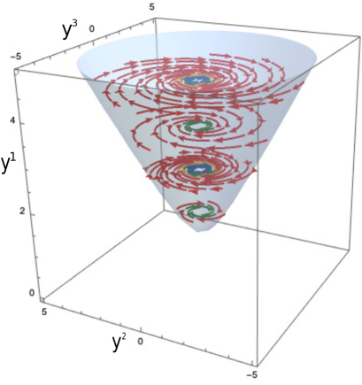
Figure 5: The GKLS vector field for a harmonic oscillator system with Hamiltonian $\hat{H}_{\tiny\mbox{Osc}}=2\,\hat{L}^{1}$ and a dissipative term introduced through the operator $v_{1}=\frac{\sqrt{\gamma}}{\hbar}\,\hat{L}^{1}$ is displayed. Here we have the frequency of oscilation $\omega=1$ and we consider the damping parameter $\gamma=1$.

The GKLS vector field is plotted in Fig. 5 where the damping parameter has been set as unity, $\gamma=1$. In this figure we observe that, regardless the initial conditions, the vector field converges asymptotically to the line $(y^{1},0,0)$, which is a singular line for $\Gamma$. Moreover, we see that the pure coherent state given by the point $(1,0,0)$ will not be affected by this dynamics.

As a second example of damping, we consider again the harmonic oscillator system in Eq. (215), but now the dissipation term is given by

$$\hat{v}_{1}=\sqrt{\gamma}\hat{K}_{+}\,,$$ (222)

where the operators $\hat{K}_{+}$ and $\hat{K}_{-}$ are given in terms of the ${\mathfrak{sl}}(2,{\mathbb{R}})$ generators as

$$\hat{K}_{+}=\frac{1}{{\rm i}\hbar}\left(\hat{L}^{3}+{\rm i}\,\hat{L}^{2}\right)\quad\text{and}\quad\hat{K}_{-}=\frac{1}{{\rm i}\hbar}\left(\hat{L}^{3}-{\rm i}\,\hat{L}^{2}\right)\,,$$ (223)

and are such that $\hat{K}_{-}=\hat{K}_{+}^{\dagger}$. Thus, by direct calculation we find that $\hat{V}=\gamma\hat{K}_{-}\,\hat{K}_{+}=\frac{\gamma}{\hbar}(\hat{L}^{0}-\hat{L}^{1})$ and then, the gradient-like vector field can be computed by means of the result in (187)

$$Y_{V}=\frac{\gamma}{\hbar}\left[({y^{1}}^{2}-1)\frac{\partial}{\partial y^{1}}+y^{1}y^{2}\frac{\partial}{\partial y^{2}}+y^{1}y^{3}\frac{\partial}{\partial y^{3}}\right]\,.$$ (224)

From (212) and (213) we find that the Choi-Kraus term is

$$Z_{\mathcal{K}}=\gamma\left({y^{1}}^{2}-y^{1}+1\right)\,\frac{\partial}{\partial y^{1}}+\gamma\,\left(y^{1}y^{2}-\frac{y^{2}}{2}\right)\,\frac{\partial}{\partial y^{2}}+\gamma\,\left(y^{1}y^{3}-\frac{y^{3}}{2}\right)\,\frac{\partial}{\partial y^{3}}\,.$$ (225)

Finally, the dynamical evolution is determined by the GKLS vector field $\Gamma=X_{H}-\hbar\,Y_{V}+Z_{\mathcal{K}}$, whose Cartesian coordinate expression is

$$\Gamma=-\gamma\left(y^{1}-2\right)\,\frac{\partial}{\partial y^{1}}-\left(\frac{\gamma}{2}\,y^{2}-2y^{3}\right)\,\frac{\partial}{\partial y^{2}}-\left(\frac{\gamma}{2}\,y^{3}+2y^{2}\right)\,\frac{\partial}{\partial y^{3}}\,.$$ (226)

Notice that the components in the direction of $y^{2}$ and $y^{3}$ are equal to those in the GKLS vector field in (219) in the previous example; however, in this case, there is a non-vanishing component in the $y^{1}$ direction. The integral curves of this vector field are solutions to the linear system of equations

$$\dot{y}^{1} =-\gamma\,(y^{1}-2)\,,$$

$$\dot{y}^{2} =-\frac{\gamma}{2}\,y^{2}+2y^{3},$$ (227)

$$\dot{y}^{3} =-\frac{\gamma}{2}\,y^{3}-2y^{2}\,,$$

and are given by

$$y^{1}(t) =(y^{1}_{0}-2)e^{-\gamma t}+2,$$

$$y^{2}(t) =e^{-\frac{\gamma}{2}t}\left(y^{2}_{0}\cos 2t+y^{3}_{0}\sin 2t\right),$$ (228)

$$y^{3}(t) =e^{-\frac{\gamma}{2}t}\left(y^{3}_{0}\cos 2t-y^{2}_{0}\sin 2t\right)\,,$$

where again $(y^{1}_{0},\,y^{2}_{0},\,y^{3}_{0})$ are initial conditions at $t=0$. The GKLS vector field for this case is displayed in Fig. 6; here we observe that there is a unique singular point at $(2,0,0)$. For any initial condition, every solution converges asymptotically to this singular point.

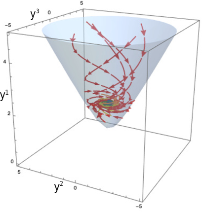
Figure 6: In this figure we plot the GKLS vector field for a Hamiltonian oscillator system $\hat{H}_{\tiny\mbox{Osc}}=2\,\hat{L}^{1}$ with dissipative part introduced through the operator $\hat{v}_{1}=\sqrt{\gamma}\,\hat{K}_{+}$. Here we have considered the Cartesian coordinates $(y^{1},y^{2},y^{3})\in\mathbf{H}$ and the damping parameter $\gamma=1$.

IV Conclusions and perspectives

In this work, we have obtained in detail the GKLS vector field for systems described by Gaussian states. In the first part, we have reviewed thoroughly the case of two-level systems, the q-bit, to introduce the concepts and procedures presented in Ciaglia-2017 , which are necessary to accomplish the same task for the dissipative dynamics of Gaussian case. Although the two cases can be worked out similarly some differences that must be taken into account. In both cases, we start by introducing the space of quantum states and recognize these as parametrized spaces, that can be described as a manifold with boundary. The purity condition $\rho^{2}=\rho$ determines the boundary of the manifold of states, while the non-pure condition ${\rm Tr}\{\rho^{2}\}<1$ its interior, that is, the boundary is the space of pure states and the open interior describes non-pure ones. As a first distinct feature, the manifold representing the quantum states for the q-bit is compact, while in the case of the Gaussian system is open, where the isospectral submanifolds are hyperboloids (112) instead of Bloch spheres.

To describe a dynamical evolution that allows a change in the degree of purity of the states, we have determined the GKLS vector field. The integral curves of this vector field are, in general, transversal to the foliation, making it possible to evolve from a pure or non-pure state to another non-pure one. This was done consistently, imposing that the orbits of this vector field were constrained to remain in the space of quantum states. To find the GKLS vector field in the Gaussian case, we followed closely the construction for the $n$-levels systems presented in Ciaglia-2017 . Thus, we considered the description of the space of quantum states from an observable point of view, which offers the advantage of endowing the space of observables with a Lie-Jordan algebra structure. In particular, for the Gaussian density matrix case, we restricted our study to operators quadratic in the position and momentum operators.

The space of observables, that is, the space of real functions on the dual of the Lie-Jordan algebra provides a realization of the Lie-Jordan algebra of operators, thus, it is possible to define geometric structures on the space of observables from these algebraic products. Namely, associated with the Lie product it is possible to define a (skew-symmetric) Poisson bivector field and to the Jordan product a corresponding symmetrical bivector. The Poisson bivector field endows the space of states with a Poisson structure and a Hamiltonian vector field can be defined for the entire space, generalizing the symplectic structure, in particular, for the case of odd-dimensional spaces. On the other hand, the symmetric bivector field defines a gradient-like vector field that is transverse to the leaves of the foliation. To constraint the orbits associated with the Hamiltonian and gradient-like vector fields to the space of quantum states, it is necessary to define such tensors in this space employing a reduction procedure. This reduction allows us to find a new symmetric bivector which yields a vector field that is transverse to the foliation, but it is tangent to the leaf of pure states.

The orbits of the vector field defined from this modified bivector defines a dynamics such that a pure state remains pure under this evolution. To amend this, a vector field associated with a completely positive map from the dual space to itself is introduced, defining in this way the GKLS vector field associated with the corresponding GKLS operator. Obviously, in the Gaussian case, the GKLS vector field is different from the one for the q-bit. It is worth mention that, to obtain the GKLS vector field for Gaussian density states we have defined a new non-Hermitian operator (189) in terms of the algebra generators to establish the mapping (190) between operators in the algebra and linear functions in its corresponding dual algebra. This operator allows to reproduce the expectation value through a simple operation; hence, it is a simpler but equivalent way of establishing the relation between an operator and its dual.

Therefore, we have shown that, in the case of states described by a Gaussian state, the GKLS dynamics also admits a decomposition principle, i.e. a conservative-Hamiltonian part as a reference dynamics, while the sum of the gradient-like and the Choi–Kraus vector fields are considered as “perturbation terms” associated with dissipation. In this sense, we have seen that the very concept of dissipation is not associated with the GKLS vector field itself, but rather, with the decomposition of this vector field in terms of the relevant geometrical structures: the Hamiltonian vector field, the like-gradient vector field and the Choi–Kraus vector field.

There are still many investigations to pursue in the study of the evolution of GKLS for Gaussian density matrices. For instance, an immediate question is whether this procedure can be generalized to address systems with more dimensions. The generalization of this procedure to $n$-levels has been already obtained in Ref. Ciaglia-2017 , while the general form of the Gaussian density matrix with a statistical mixture for $n$-dimensions is well known and has been constructed employing a generalization of the so-called covariance matrix, see Ferraro-2005 and references therein. Thus, taking into account these results one could proceed directly to construct the GKLS vector field for more degrees of freedom. This will be presented in a forthcoming work.

Another important generalization of our procedure is to consider the Gaussian states with non-vanishing first moments. This implies considering observables at most quadratic in position and momentum operators, i.e., one may include linear operators such as the creation and annihilation operators. However, including linear operators means that we are no longer dealing with the ${\mathfrak{sl}}(2,{\mathbb{R}})$ Jordan–Lie algebra, but rather with a semidirect product of algebras, specifically, the ${\mathfrak{sl}}(2,{\mathbb{R}})$ and the Heisenberg-Weyl algebra. Then, given this kind of system, one may try to obtain the GKLS vector field following the procedures in this paper. This will be studied in a future work.

Finally, in this work, we have only considered as a fiducial state the Gaussian density matrix, so a natural question is: whether different fiducial states can be chosen? In particular, it might be possible to consider the following Wigner function. Let us define

$$I(q,p,t):=\frac{4}{\hbar^{2}\,r^{2}}\left[\sigma_{p}^{2}q^{2}-2\sigma_{qp}qp+\sigma_{q}^{2}p^{2}\right]\,,$$ (229)

then, one may introduce the following family of Wigner functions

$$W_{n}(q,p)=\frac{(-1)^{n}}{\pi\,\hbar\,r}e^{-\frac{1}{2}I(q,p,t)}L_{n}[I(q,p,t)]\,,$$ (230)

where $L_{n}$ denotes the Laguerre polynomials. Then, $r=1$ corresponds to Wigner functions associated with the Fock states; however, for $r\neq 1$ these states satisfy the Robertson–Schrödinger uncertainty relation

$$\sigma_{q}^{2}\,\sigma_{p}^{2}-\sigma^{2}_{qp}=\frac{\hbar^{2}\,r^{2}}{4}\,,$$ (231)

and the purity condition

$${\rm Tr}\{\hat{\rho}^{2}\}=\frac{1}{r}\,.$$ (232)

Notice that, $n=0$, returns the Gaussian density matrix studied in this work. This set of states has the same space of parameters analyzed for the Gaussian density matrix and then our results might be applied directly, i.e., the GKLS vector field obtained in (214) could be used with fiducial states in the set $\{W_{n}(q,p)\}$. These results will be studied in future contributions.

V References

References

• (1) F. Strocchi, Rev. Mod. Phys., 38 (1) (1966).
• (2) V. Cantoni, Rendiconti del Seminario Matematico e Fisico di Milano, 48 (1978) 35–42.
• (3) P. Kramer and M. Saraceno, Geometry of the time-dependent variational principle in quantum mechanics (Springer-Verlag, Berlin Heidelberg, 1980).
• (4) R. Cirelli, P. Lanzavecchia and A. Mania, J. Phys. A: Math. Gen., 16 (16) (1983) 3826.
• (5) M. Moshinsky and C. Quesne, J. Math. Phys., 12 (8) (1971) 1772–1780.
• (6) P. A. Mello, M. Moshinsky, J. Math. Phys., 16 (10) (1975) 2017–2028.
• (7) P. A. M. Dirac, The principles of quantum mechanics (Oxford university press, 1981)
• (8) J. Grabowski, M. Kuś, and G. Marmo, J. Phys. A Math. and Theor., 38 (2005) 10217.
• (9) P. Aniello, J. Clemente-Gallardo, G Marmo, G. F. Volkert, (2011) arXiv preprint arXiv:1101.0625.
• (10) F. M. Ciaglia, F. Di Cosmo, A. Ibort, M. Laudato and G. Marmo, Open Syst. Inf. Dyn. 24 (3) (2017) 1740003.
• (11) D. Chruściński, F. M. Ciaglia, A. Ibort, G. Marmo, and F. Ventriglia, Ann. Phys, 400 (2019) 221–245.
• (12) V. Gorini, A. Kossakowski, and E. C. G. Sudarshan, J. Math. Phys., 17 (1976) 821.
• (13) G. Lindblad, Commun. Math. Phys., 48 (1976) 119.
• (14) I. A. Malkin, V. I. Man’ko and D. A. Trifonov, Phys. Lett. A, 30 (1969) 414.
• (15) I. A. Malkin, V. I. Man’ko and D. A. Trifonov, J. Math. Phys., 14 (5) (1973) 576–582.
• (16) A. M. Perelomov, Commun. Math. Phys., 26 (1972) 222.
• (17) F. T. Arecchi, E. Courtens, R. Gilmore, and H. Thomas, Phys. Rev. A, 6 (6) (1972) 2211–2237.
• (18) E. Onofri, J. Math. Phys., 16 (1975) 1087–1089.
• (19) V. I. Man’ko, G. Marmo, E. C. G. Sudarshan, and F. Zaccaria, Phys. Scripta, 55 (1997) 528.
• (20) P. Aniello, V. Man’ko, G. Marmo, S. Solimeno, and F. Zaccaria, J. Opt. B Quantum semiclass, 2 (2000) 718–725.
• (21) P. Aniello, G. Marmo, and G. F. Volkert, Int. J. Geom. Meth. Mod. Phys., 07 (2009) 369–383.
• (22) H. Cruz-Prado, G. Marmo, D. Schuch and O. Castaños, J. Math. Phys., 62 (4) 042105.
• (23) A. Ferraro, S. Olivares and M. A. G. Paris, Gaussian states in continuos variables quantum information (Napoli Series on physics and Astrophysics, Bibliopolis Naples, 2005).
• (24) M. O. Scully and M. S. Zubairy, Quantum Optics (Cambridge University Press, Cambridge, UK, 1999).
• (25) J. M. Radcliffe, J. Phys. A, 4 (1971) 313.
• (26) A. M. Perelomov, Soviet Physics Uspekhi, 9 (1977) 703.
• (27) E. Ercolessi, G. Marmo, G. Morandi, From the equations of motion to the canonical commutation relations, RIV. NUOVO CIMENTO 33 (8) (2010)
• (28) W. M. Zhang, D. H. Feng and R. Gilmore, Robert, Rev. Mod. Phys., 62 (1990) 867.
• (29) H. Cruz-Prado, G. Marmo and D. Schuch, J. Phys. Conf. Ser., 1612 (2020) 012010.
• (30) V. I. Arnol’d, Mathematical methods of classical mechanics, (Springer Science & Business Media, 2013).
• (31) K. Kraus, Ann. Phys., 64 (1971) 311.
• (32) M. D. Choi, J. Canad. Math., 24 (1972) 520.
• (33) M. D. Choi, Lin. Alg. Appl., 10 (1975) 285.
• (34) J. F. Cariñena, A. Ibort, G. Marmo and G. Morandi, Geometry from dynamics, classical and quantum. (Springer-Verlag, Berlin, Heidelberg, New York, Tokyo, 2015).
• (35) H. Weyl, The Theory of Groups and Quantum Mechanics (Dover Publications, New York, 1950).
• (36) H. Cruz, D. Schuch, O. Castaños and O. Rosas-Ortiz, Ann. Phys., 360 (2015) 44-60.
• (37) N. L. Balazs and A. Voros, Phys. Rep., 143 (3) (1986) 109-240 .
• (38) C. L. Siegel, Am. J. Math., 22 (1) (1943) 1–86.
• (39) R. Simon, E. C. G. Sudarshan, and N. Mukunda, Phys. Rev. A 36 (1987) 3868.
• (40) H. A. Kastrup, Fortschritte der Physik: Progress of Physics, 51 (10-11) (2003) 975–1134.
• (41) Lie Methods in Optics, Proceedings of the CIFMO-CIO Workshop Held at León, México, January 7-10, 1985 (Springer-Verlag, Berlin, Heidelberg, New York, Tokyo, 1986)
• (42) A. P. Balachandran, S.G. Jo and G. Marmo, Group Theory and Hopf Algebras: Lectures for Physicists (World Scientific 2010).