How planets form by pebble accretion
V. Silicate rainout delays contraction of sub-Neptunes
The characterization of Super-Earth-to-Neptune sized exoplanets relies heavily on our understanding of their formation and evolution. In this study, we link a model of planet formation by pebble accretion (Ormel et al., 2021) to the planets’ long-term observational properties by calculating the interior evolution, starting from the dissipation of the protoplanetary disk. We investigate the evolution of the interior structure in 5–20planets, accounting for silicate redistribution caused by convective mixing, rainout (condensation and settling), and mass loss. Specifically, we have followed the fate of the hot silicate vapor that remained in the planet’s envelope after planet formation, as the planet cools. We find that disk dissipation is followed by a rapid contraction of the envelope from the Hill/Bondi radius to about one-tenth of that size within 10 Myr. Subsequent cooling leads to substantial growth of the planetary core through silicate rainout, accompanied by inflated radii, in comparison to the standard models of planets that formed with core-envelope structure. We examine the dependence of rainout on the planet’s envelope mass, distance from its host star, its silicate mass, and the atmospheric opacity. We find that the population of planets formed with polluted envelopes can be roughly divided in three groups, based on the mass of their gas envelopes: bare rocky cores that have shed their envelopes, super-Earth planets with a core-envelope structure, and Neptune-like planets with diluted cores that undergo gradual rainout. For polluted planets formed with envelope masses below 0.4, we anticipate that the inflation of the planet’s radius caused by rainout will enhance mass loss by a factor of 2–8 compared to planets with non-polluted envelopes. Our model provides an explanation for bridging the gap between the predicted composition gradients in massive planets and the core-envelope structure in smaller planets.
Key Words.:
Planets and satellites: formation – Planets and satellites: interiors – Planets and satellites: composition –1 Introduction
The mass-radius relation of exoplanets (i.e., bulk density) depends on their composition, but also on composition distribution in the interior. Here, mixtures of elements are usually more compact than separate composition layers (e.g., Baraffe et al., 2008; Fortney et al., 2013; Dorn & Lichtenberg, 2021). In particular, the mass-radius relation of silicate-dominated planets with only a few percent of gas are more sensitive to the thermal evolution of the metal-rich interior (Lopez & Fortney, 2014; Vazan et al., 2018a, b) and to the mean molecular weight (pollution) of the gas envelope.
Observations from online and upcoming facilities as JWST (Greene et al., 2016), PLATO (Rauer et al., 2014) and ARIEL (Tinetti et al., 2018) space telescopes are expected to provide high quality data as well as improved statistics for stellar ages (PLATO) and atmospheric compositions (ARIEL, JWST). One way to shed light on the nature of these planets is by studying the sequence of planet formation and long term thermal evolution. While planet formation sets the initial mass and composition of the planet, the long term evolution connects it to the observed properties.
Planet formation models that follow the solid deposition in the interior show that most of the accreted metals are distributed in the gas envelope once the planet exceeds about 2, due to solid-gas interaction in the growing envelope (Bodenheimer et al., 2018; Brouwers et al., 2018; Valletta & Helled, 2019; Brouwers & Ormel, 2020; Ormel et al., 2021; Steinmeyer et al., 2023). Thus, formation-evolution of 5-20rocky planets involve the evolution of polluted envelopes, usually with non-uniform distribution of metals in it.
A question that arises is whether such a non-uniform structure is stable on timescales where these planets are observed – i.e., several Gyr – or whether the internal state has been re-arranged into a standard core-envelope structure (”standard” refers to how these planets are typically perceived) or something in between (i.e., compositional layers). Processes in the interior like mixing or settling redistribute matter along with the thermal evolution of the planet. If convection is vigorous convective-mixing can erode the initial metal distribution and homogenize it (Vazan et al., 2015). Alternatively, progressive cooling can lead to over-saturation in the polluted envelope and rainout (condensation and settling) of silicate droplets to deeper hotter layers (Brouwers & Ormel, 2020). Thus, the planetary structure directly after formation is not necessarily the structure at the present-day111Compositional diffusion might also change the planetary structure, but is found to be negligible in comparison to convective-mixing and rainout, as is shown in section 2.4..
Evolution models usually use arbitrary initial conditions. While this is a fair assumption for interior models of 2-3 homogeneous composition layers, it cannot hold for evolution of planets with non-uniform composition distribution. When composition in planets after their formation is not uniformly distributed, evolution is not adiabatic (Ledoux, 1947; Rosenblum et al., 2011), and hence thermal evolution is sensitive to initial conditions (i.e., formation outcomes).
In Ormel et al. (2021) we found that rocky 5-20planet formed by pebble accretion have a typical structure of a small rocky core surrounded by a silicate vapor composition gradient and a vapor-rich (¿40%) convective envelope on top of it. In that work Phase IV was defined as the phase where the protoplanetary disk dissipates, the outer layers of the atmosphere may evaporate, and where progressive cooling may cause the vapor to rain out. Here we aim to model this phase.
In a recent Letter (Vazan & Ormel, 2023) we show that condensation and settling (rainout) of silicates in the envelope of sub-Neptune planets have a noticeable effect on their observed radii. In this paper we generalize this study to a wider range of planetary masses and conditions, and denote the trends in evolution of polluted envelopes. We calculate the long term properties of 5-20rocky planets composed of silicate, hydrogen and helium, that formed via pebble accretion. The model contains: (1) initial interior structure from planet formation model, (2) thermal evolution including relevant heat transport mechanisms and energy sources, (3) structural evolution (material transports) by convective-mixing and settling, (4) gas mass loss from young atmospheres.
2 Method
2.1 Formation-Evolution interface
Our initial models are the resulting interior models of Ormel et al. (2021) for planet formation by rocky pebble accretion. At the end of the formation phase the young planet is embedded in the disk, and its radius is of the order of hundred Earth radii (Bondi radius / Hill radius). The interior of the young planet is typically structured in four stable layers: a small rocky core (1-2), a silicate vapor composition gradient, a uniform silicate-rich convective envelope, and a thin silicate-poor saturated atmosphere.
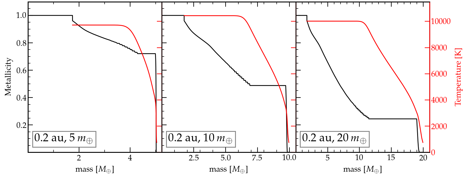
In Figure 1 we present the silicate distribution (Z) and temperature profile of planets at the end of their formation phase. The formation models in the figure are calculated for accretion of 1 mm rocky () pebbles, at a solid accretion rate of yr-1, where opacity in the formation phase is of gas and pebbles. In section 3.6 we discuss how varying these parameters affects the results. The parameters from the formation model that we use in the evolution calculation are interior profile of temperature, density, luminosity, entropy, and composition (species mass fraction).
In our simulation the transition from disk phase to post-disk long term evolution is sharp, as the formation outcome model is the input of the evolution model. Specifically, the pressure at the outer boundary is now given by the photospheric conditions, which is significantly lower than the disk pressure. The temperature at the outer boundary is determined by the distance from the (sun-like) star, which is unchanged between formation and evolution.
For consistency of the thermal evolution model with the planet formation model we use the same set of equations of state for hydrogen and helium (Saumon et al., 1995), and rock (Faik et al., 2018). Irradiation by the parent star is for the same location as in the disk phase (i.e., no migration). We evolve formation models of planets at distances of 0.2 AU and 1 AU from a sun-like star222Planets at larger distances are expected to contain significant amount of volatiles and thus are beyond the scope of this work.. The number of mass grid points is reduced by interpolation to 500, which is optimal for the thermal evolution code runs.
2.2 Thermal evolution model
The interior thermal evolution code is a Henyey-like333An iterative implicit integration method for boundary value problems, in which the structure equations are solved together with the evolution equations (Henyey et al., 1964). code that solves the set of structure-evolution equations simultaneously on an adaptive grid of mass from center to surface (Kovetz et al., 2009). Thus, the thermal state of the deep silicate core, including its compression and cooling is integral part of the evolution scheme. At each mass grid-point we obtain a solution for the equations of continuity (1), hydrostatic equilibrium (2), energy transport via convection, radiation, and conduction (3), energy balance (5), and composition flux (5):
| (1) |
| (2) |
| (3a) | |||
| where the symbols are the radius, mass, density, pressure and temperature respectively. is the temperature gradient determined by the heat transport mechanism according to the Ledoux convection criterion (Ledoux, 1947): | |||
| (3b) |
is the adiabatic gradient,
| (3c) |
is the composition dependent gradient,
| (3d) |
where is mass fraction of the th species.
is the radiative (and/or conductive) temperature gradient,
| (3e) |
is the radiation pressure, luminosity, is the harmonic mean of radiative () and conductive () opacities:
| (3f) |
Grains or pebbles are not expected to remain in the upper envelope after the formation phase (Brouwers et al., 2021; Movshovitz et al., 2010; Ormel, 2014; Mordasini, 2014), and therefore we use the radiative opacity of Freedman et al. (2014) for grain-free atmospheres. The opacity in each layer is calculated for the layer’s given pressure-temperature-metallicity values. However, since in practice atmospheric metallicity composed of various elements, and not solely of silicate vapor that we consider in this work, we apply the condition
| (4) |
as the metallicity for which the Freedman opacities are calculated. Here, we take equal to the solar metallicity by default. Note that while is fixed throughout the simulation, is calculated based on the L-V curve (eq. 9). Thus, in layers where the silicate vapor fraction drops below solar the solar metallicity is adopted for the calculation of the opacity. Conduction is governed by the silicate component, as molecular hydrogen is poor conductor (French et al., 2012) and pressure-temperature in interiors of super-Earths are below the metallic hydrogen level. Conductive opacity is obtained by extrapolation of Earth rock parameters to high pressure and temperature as described in appendix B.
is the temperature gradient calculated by the Mixing Length Recipe (MLR) (Mihalas, 1978; Kippenhahn et al., 2013), where turbulent Rayleigh-Bénard convection is simulated in 1D. We take the size of a convective cell to be half the local scale height444See Vazan et al. (2015) for more details on the MLR model and on the effect of its parameters on results..
The energy balance in the interior is according to
| (5) |
where specific energy (), contraction, and contribution of radiogenic heating in the rock (), are considered.
| Material transport by convective mixing is calculated as a diffusive-convective flux of particles (Kippenhahn et al., 2013): | |||
| (6a) | |||
| where is the number fraction of the th element, namely the mass fractions divided by the atomic mass of the element, and is the particle flux of the th element: | |||
| (6b) |
| (6c) |
The particle flux is determined by a diffusive coefficient , which depends on the convection velocity and mixing length .
At every mass layer and timestep the equation of state for a mixture of the three materials - hydrogen, helium (H, He) and silicate () - is calculated according to the additive volume law
| (7) |
where is the density of the th species, obtained from the equation of state (H,He from Saumon et al. (1995) and from Faik et al. (2018)). The other thermodynamic properties of the mixture are calculated as described in Vazan et al. (2013).
2.2.1 Rainout model
As the planet cools the vapor in the envelope become oversaturated, and part of it condensates and settles down to deeper hotter (undersaturated) layers. The processes sweeps the silicate from the outer layers downwards and gives rise to late core growth. The rainout phase terminates when all silicates have settled into a silicate core surrounded by a metal-poor hydrogen-helium envelope555We ignore residuals of less than 2% in mass that may stay in the envelope.. Once the core-envelope structure has been established, the structure is static and further cooling doesn’t affect the composition distribution. We define the rainout timescale as the time from disk dissipation until all silicates have settled and a core-envelope structure has been established.
Settling from an supersaturated layer into a deeper undersaturated layer is assumed to be instantaneous, since the settling timescale of a silicate droplet is orders of magnitude smaller than the evolution timescale (see Section 2.4 below). For the same reason we exclude the possibility of supersaturation. We model rainout numerically by removing the excess of silicate (the amount above the saturation metallicity) from a layer to the layer below it . Between timestep and , whenever the pressure-temperature in the layer () are such that we take:
| (8a) | |||
| and the excess amount of silicate is moved from the layer to the layer below it, enhancing its metallicity: | |||
| (8b) | |||
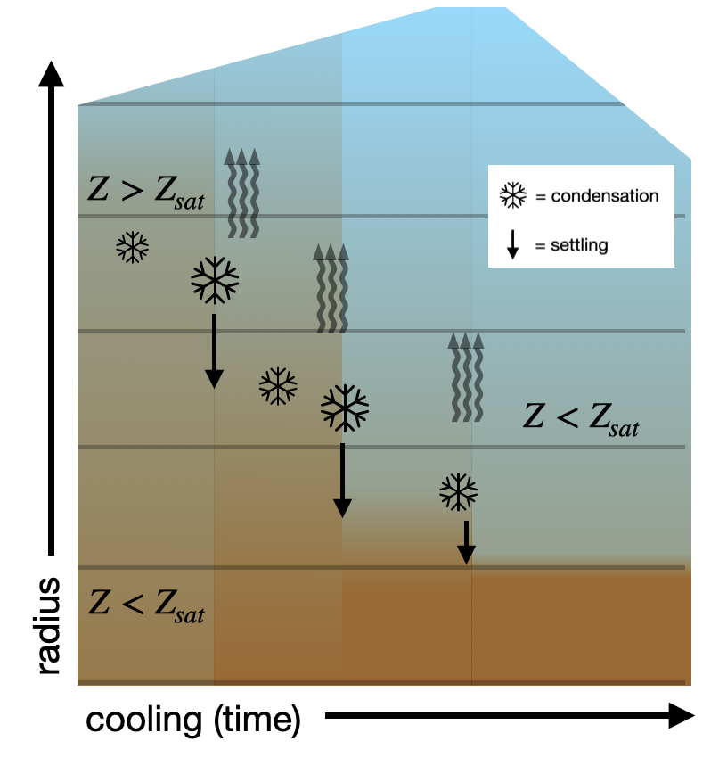
The rainout of silicate releases energy – latent heat of condensation and gravitational energy of settling. An additional energy source is the late release of the heat from formation that is liberated after the compositional gradient has been erased. This energy is more difficult to estimate as it varies with formation conditions. The energy change by rainout is included in our equation scheme: the energy of condensation (latent heat) is part of the equation of state, the energy of settling (gravitational energy) is obtained by the structure equations, and the release of heat from formation is calculated self-consistently by the evolution model. A schematic sketch of the rainout process and its energetic contribution to the thermal evolution appear in figure 2.
The saturation criterion is defined by silicate liquid-vapor (L-V) curve (e.g. Podolak et al., 1988; Bodenheimer et al., 2018; Stevenson et al., 2022). For consistency with our formation model (Ormel et al., 2021) we use the fit of L-V curve (lower branch) of Kraus et al. (2012):
| (9) |
in cgs units, where , K, , and K.
2.2.2 Atmosphere model and mass loss estimate
The atmosphere in our model is gray and plane-parallel, and the temperature distribution is calculated for a vertical (maximal) irradiation flux, with no angle dependency of the incident flux (e.g., Guillot, 2010). The temperature in the atmosphere follows:
| (10) |
where is optical depth, the outgoing energy flux, (Kaniel & Kovetz, 1967), and is Stefan-Boltzmann’s constant.
The atmospheric boundary is the planetary photosphere, with optical depth . The net outward luminosity from the surface of the planet is
| (11) |
The irradiation temperature as a function of the distance from the star is
| (12) |
where is the stellar luminosity, here taken to be solar, is the planet-star orbital separation, and is the bond albedo.
Mass loss is simulated as material escape from the outermost layer in a given rate. The outermost layer is poor in silicate vapor, due to efficient rainout and atmospheric temperatures well below silicate evaporation (). Therefore the mass loss (removal) is assumed to be of hydrogen-helium.
2.3 Analytical estimate for the rainout timescale
Brouwers & Ormel (2020) analytically estimated rainout timescales for super-Earth planets. Their calculation assumes an ideal gas equation of state, constant opacity and luminosity, and adiabatic cooling. It is calculated for a three layers structure of a constant density core, an intermediate uniform polluted envelope, and an outer hydrogen envelope.
Here, we adopt a slightly modified form of the estimate of Brouwers & Ormel (2020) for the sedimentation timescale. We estimate the energy available for rainout as
| (13) |
where and are the core mass and total heavily element mass, respectively, and and are the radii corresponding to these masses and is the latent heat per unit mass of silicate (SiO2) condensation. In Brouwers et al. (2018) and Ormel et al. (2021) it has been shown that is an appropriate choice for the (solid) core mass after formation; the heavy element mass above this point () will be vaporized. In Eq. (13) the two cases correspond to the limits where is small, in which case the gravitational potential is determined by the , and where is large, respectively. The sedimentation luminosity follows Brouwers & Ormel (2020):
| (14) |
where is the radiative-convective boundary (RCB) temperature, set to be the evaporation temperature , is the radiative opacity at the radiative atmosphere, is the core density, and is the gas (H,He) mass. is the modified Bondi radius
| (15) |
where and are the gas adiabatic index and mean molecular weight respectively, and is Boltzmann’s constant.
From this we can calculate a rainout time
| (16) |
The values of the model parameters appear in Table 1.
| parameter | symbol | value |
|---|---|---|
| gas adiabatic index | 1.45 | |
| mean molecular weight | 2.35 | |
| silicate evaporation temperature | Tvap | 2500 K |
| radiative opacity | 0.1 cm2/g | |
| latent heat | ulat | 1.5erg/g |
| core density | 5 g/cm3 | |
| initial core mass | 2 |
2.4 Timescales of interior evolution
To give intuition on the thermal evolution of non-uniform polluted envelopes, we provide order of magnitude estimates of relevant timescales:
Settling: For silicate vapor condensation we assume rain droplets sizes of , which provides, based on Movshovitz & Podolak (2008) sedimentation velocity of , resulting in sedimentation time () of up to 200 yr, orders of magnitude below the Kelvin-Helmholtz times in the evolution model. Thus, taking settling to be an instantaneous process in our simulation is reasonable.
Mass loss: Average mass loss rate by XUV radiation from planets at 0.2 AU is about Myr-1, using standard photoevaporation model (e.g., Owen & Wu, 2013). Estimated mass loss timescale of results in timescale of yr, indicating that polluted planets in the lower mass range can lose their entire envelopes.
Conduction: Suppression of convection in the deep interior can form thermal boundaries in which heat is transported by conduction / layered-convection, where conductive transport is slower and therefore the lower bound for heat transport. The timescale for conduction in layer of thickness , density , and thermal conductivity is approximately . For heat capacity and values for density and thermal conductivity from our simulations we get . Thus, an effective thermal boundary (i.e., ) has a conductive layer of about 300 km in order to keep most of the heat from formation in the deep interior in Gyr time.
Material diffusion: Diffusion in composition boundaries can be approximate by a Brownian motion with timescale , where the length scale of the change in particle position, and diffusivity. Estimate of diffusivity by Stokes-Einstein equation , for temperature , viscosity of , and silicate () molecular size of , provides . Hence, diffusion can transport particles within Gyr to about 0.5 km. Since this upper bound of diffusion length-scale is smaller than the conductive boundary, diffusion is expected to be negligible in the interior evolution of rock dominated planets. Higher viscosity (than 1 Pas) and/or larger particles (than m) result in even slower diffusion.
3 Results
3.1 From formation to evolution
The evolution calculation starts at disk dissipation. We find that the decrease in pressure of the outermost envelope at disk dissipation does not lead to mass loss by Roche lobe overflow, unless atmospheric metallicity (opacity) is unrealistically high. If the upper atmosphere maintains a high opacity for some reason this would lead to envelope expansion and to mass loss (Ginzburg et al., 2016). However, the efficient grain settling expected in planetary atmospheres (Brouwers et al., 2021; Movshovitz & Podolak, 2008; Ormel, 2014; Mordasini, 2014) leads to grain-free atmospheres, thus low atmospheric metallicity. Using the grain-free opacity tables of Freedman et al. (2014) results in efficient cooling and no mass loss at the disk dissipation stage (see also appendix A.2 in Vazan et al., 2018b). This finding holds for all models we have tested in this work.
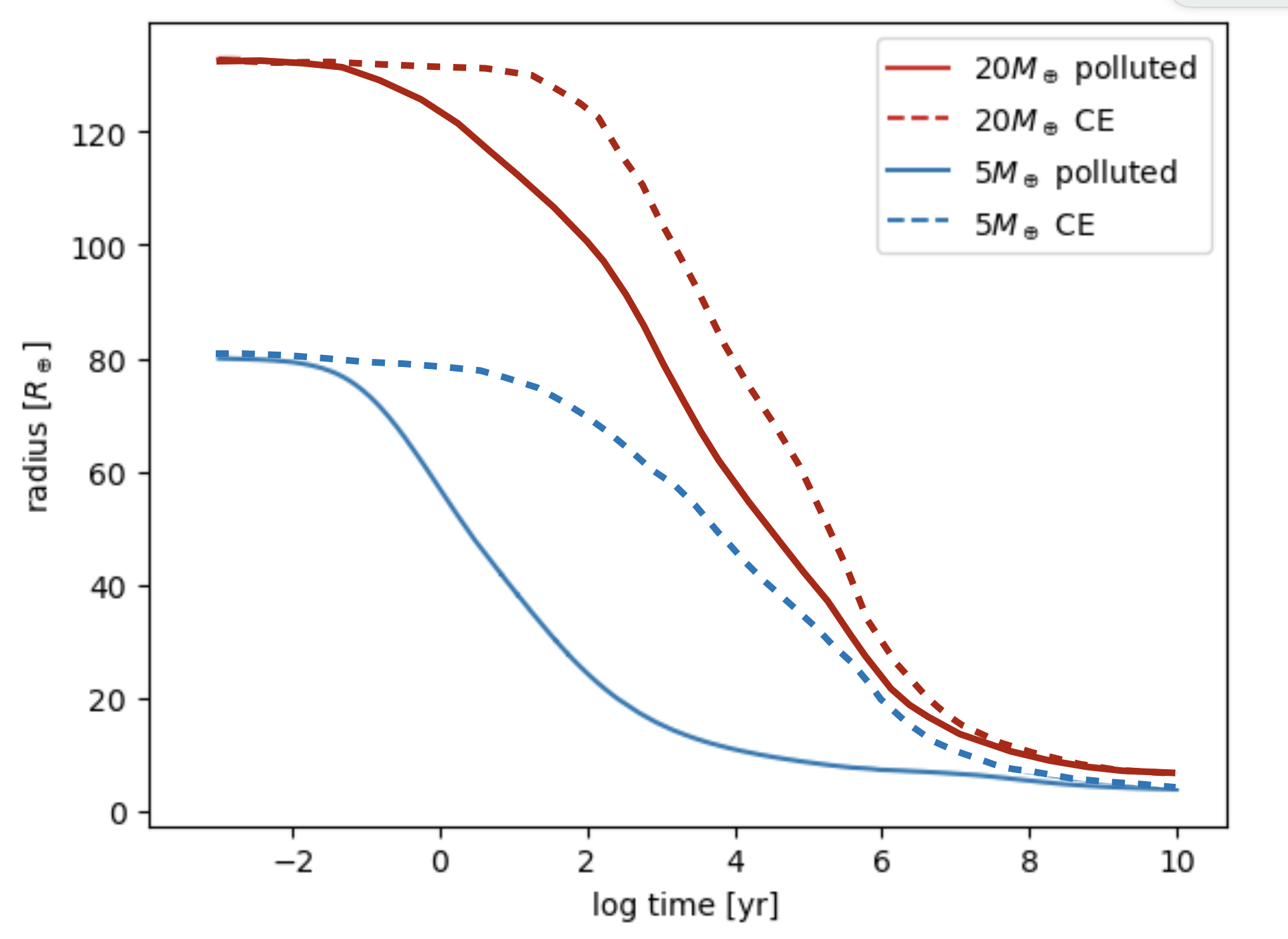
After the disk dissipates the young planet enters a phase of rapid contraction of the outer diluted envelope, in which the formed planet contracts from its Bondi / Hill radius to about a tenth of it. In figure 3 we show the radius contraction of the planets from figure 1 at 0.2 AU. For comparison, we show planets with the same composition that formed with core-envelope structure. The initial models for the core-envelope cases are of isentropic core and envelope, with same central temperature as in our formation models. Evolution time is shown in log scale to emphasis the early evolution right after planet formation ends. In general, the early rapid contraction of planets with polluted envelopes is faster than that of similar planets with core-envelope structure. The higher mean molecular weight of the polluted envelope and the slower heat transport due to the deep composition gradient (convection suppression) lead to accelerated early contraction of the polluted envelopes666This finding is for static interior structure. When silicate rainout takes place the radii of planets with polluted envelopes exceed that of planets with core-envelope structure, as will be discussed in the next sections., where the difference is greater for smaller, more-polluted, planets. Timescale for the contraction from formation radius to about tenth of it varies from a few years for the 5planets to a few years for 20planets. Higher opacity could potentially prolong the contraction time, but we find the required opacity increase unrealistically high.
3.2 Thermal and structural evolution
After the rapid contraction that heats-up the outer envelope, the planet starts to cool. The cooling of the uniform metal-rich envelope is governed by large scale convection, while the heat transport from the deeper interior - where the composition gradient acts as a thermal boundary - is less efficient. Consequently, the temperatures in the metal-rich envelope decreases to below the saturation level and silicate condensate and settle (rainout) to deeper undersaturated layer (see figure 2). The process of rainout is a top-to-bottom process, in which a complete rainout leads to a core-envelope structure.
Core erosion and mixing upwards of the silicates by convection (convective-mixing) are found to be negligible in all the planets we explored in this work, for two reasons; first, the deep composition gradients from formation are relatively steep in metal-dominated planets, and therefore are stable against convection (Vazan et al., 2022); and second, inhibition of convection by composition gradients along the saturation pressure-temperature profile suppresses redistribution of elements in saturated layers (Guillot, 1995; Markham et al., 2022).
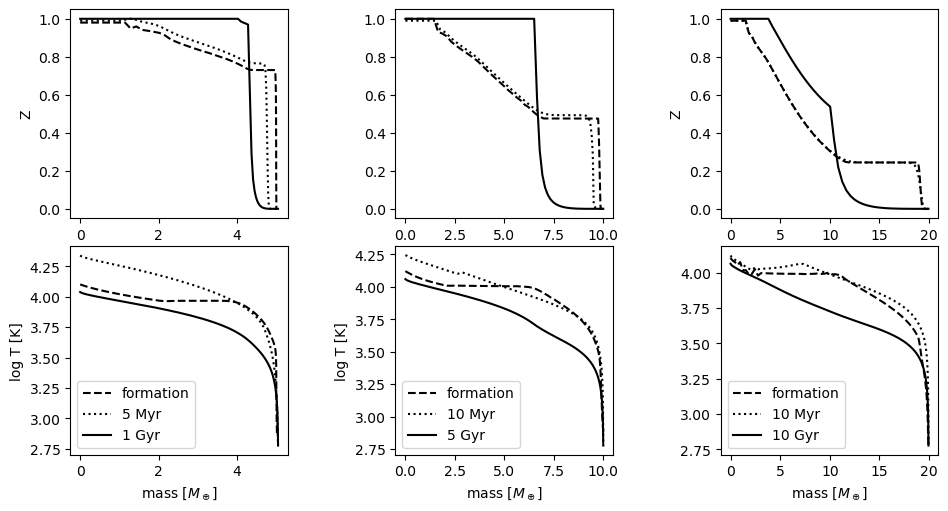
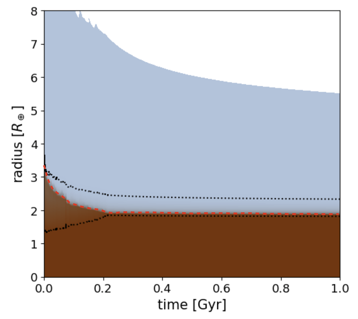
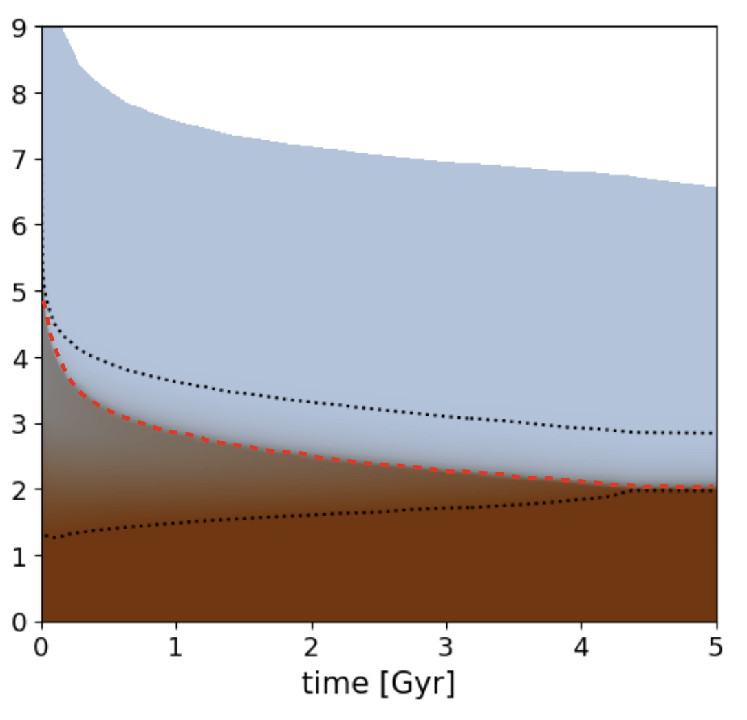
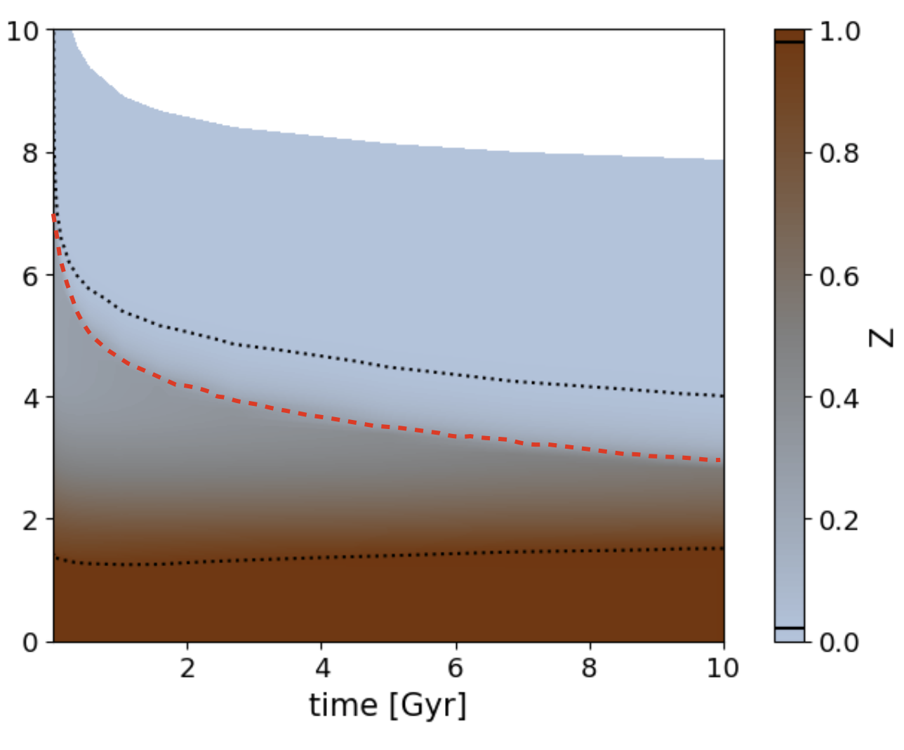
In figure 4 we show silicate mass fraction (Z) profile and temperature profile of 5(left), 10(middle), and 20(right) planets located at 0.2 AU. It shows that the early rapid contraction phase has only a small effect on the composition distribution (dotted). Despite the large change in radius, the deep interior (composition gradient and below) stays almost unchanged in this early evolution phase. In the long term cooling phase the composition distribution significantly changes by rainout. Rainout in the 10and 5planets results in a core-envelope structure before 5 Gyr and 1 Gyr, respectively. In the more massive and gas-rich 20planet rainout depletes the outer layers from silicates but yet a significant composition gradient is maintained in the deep interior after even 10 Gyr.
The structure evolution (redistribution of silicate in time) by the rainout is shown in figure 5. Rainout of silicate in the 5planet starts almost immediately after disk dissipation and ends (the planet reaches core-envelope structure) after 0.38 Gyr. The process is much slower in the gas-rich 20planet, where silicate rainout starts after 10 Myr, and is still ongoing after 10 Gyr. The 10planet is an intermediate case, in which core-envelope structure is reached after 4.25 Gyr.
3.3 Rainout dependency on envelope mass and metal mass
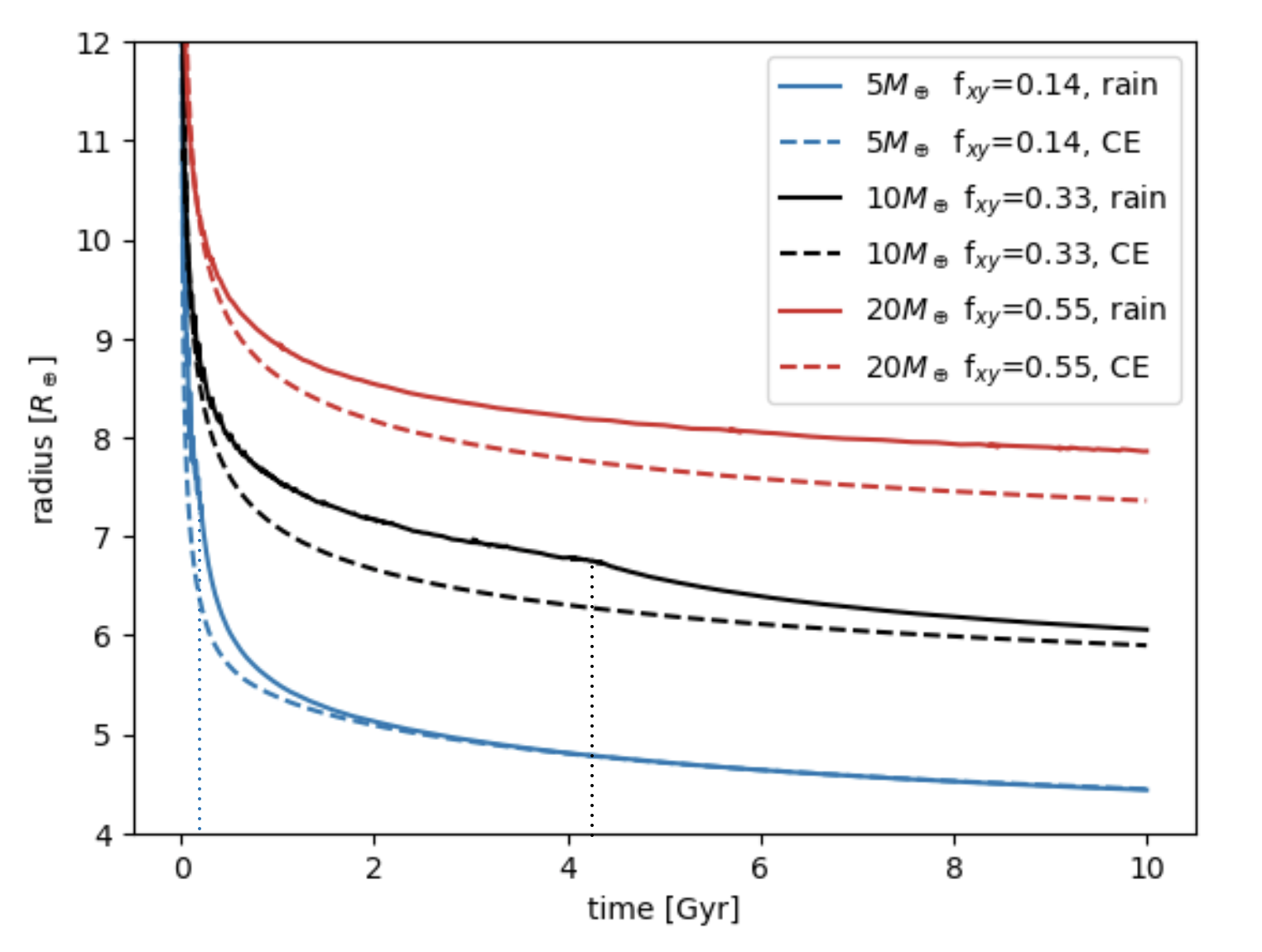
Planets with different envelope masses experience rainout at different time and strength (Vazan & Ormel, 2023). Consequently, the strength and duration of radius inflation, caused by the rainout energy release, varies; when rainout is faster, the energy release is on a shorter timescale and therefore radius expansion is larger. Rainout is faster and earlier in smaller planets, due to their lower envelope mass, larger envelope metallicity, and lower gravity. In figure 6 we show the radius evolution corresponding to the 5, 10and 20planets shown in figure 5. For comparison we also plot the radius evolution of planets of the same composition but that start off with a core-envelope structure from the outset. As can be seen, the 5planet has an early and large radius inflation by rainout, after which it becomes identical to its core-envelope twin. The 10and 20keep a moderate radius inflation in comparison to their core-envelope analogue, due to post-rainout heat release (10) and ongoing rainout (20).
Misener & Schlichting (2022) calculated structure model for planets with polluted envelopes and found that silicate vapor layer decreases the planet’s total radius compared to a similar planet with pure H,He envelope. While mean molecular weight and composition gradient (suppression of convection) arguments indeed lead to smaller radius as suggested by these authors, including the structure evolution and specifically the rainout process in thermal evolution can result in larger radius, caused by the release of rainout energy: latent heat, gravitational energy, and late release of locked formation energy.
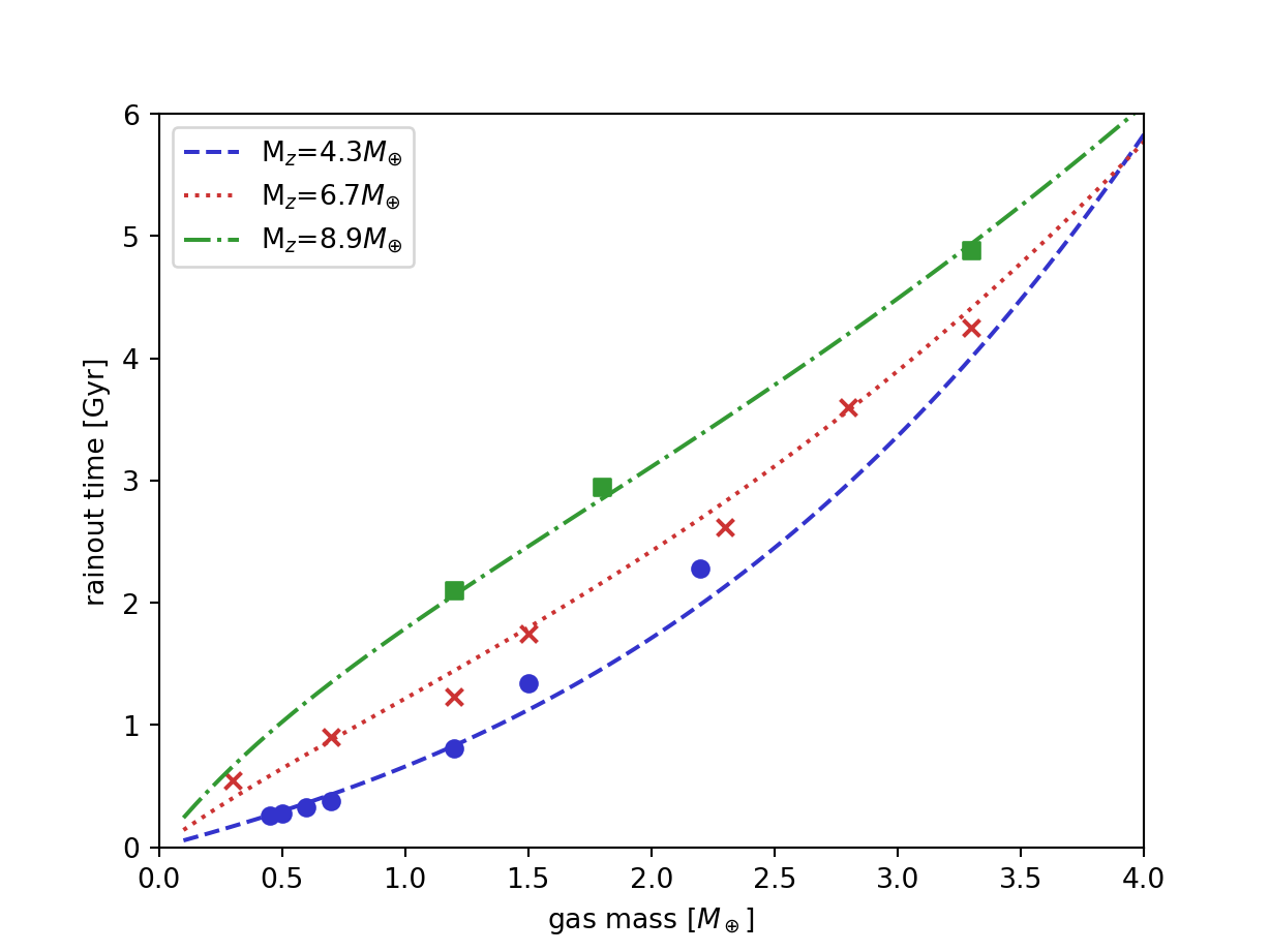
The envelope mass, more specifically the pressure-temperature at the bottom of the envelope, plays a key role for the rainout time. Planets with light envelopes experience shorter and earlier rainout than planets with massive envelopes. In Vazan & Ormel (2023) we found that an envelope mass of approximately 0.75to be an upper limit for sub-Neptunes to reach the core-envelope structure within 1 Gyr. This result was found for planets with 6.7of silicates. Here we repeat this calculation for planets with different silicate masses.
In figure 7 we show simulation results (points) of rainout timescale with gas (H,He) mass for three different cases of total silicate mass (): 4.3(blue), 6.7(red), 8.9(green). The lines are for analytical fits and will be discussed in the next section. We find that the rainout timescale increases with the total silicate mass (for same envelope mass), thus rainout takes longer in more massive planets with the same gas mass. Simulations results indicate that the change in rainout time with silicate mass is especially noticeable in planets with small gas to silicate ratio. For example, rainout in a gas envelope of 1.2H,He takes 0.81 Gyr in 5.5planet, 1.23 Gyr in 8planet, and 2.1 Gyr in 10planet. The reason is that stronger gravity in more massive planet leads to denser and hotter deep envelopes, in which silicate are undersaturated for longer. However, when gas mass is comparable to the metal mass the differences between cases diminishes, probably the result of the larger heat capacity of hydrogen and helium in comparison to rock.
3.4 Comparison to analytical calculation
We next use our detailed simulation to examine the validity of the analytical results of Brouwers & Ormel (2020) on the rainout timescale. As described in section 2.3 the analytical model contains assumptions on the structure (three layer model) and its properties (ideal gas, constant parameters), and is obtained by assuming low mass envelopes (to neglect gas gravity). The free parameter values were set as in Brouwers & Ormel (2020), and appear in table 1. The fit of the analytical calculation (equation 16) to the simulation results is found to be poor for planets with a significant gas fraction. The poor fit may be the result of neglect of envelope gravity, oversimplification of gas compression (ideal gas), and constants such as opacity, core density, and evaporation temperature. However, we obtain a much better fit to the simulation data when we take:
| (17) |
The improved fit of equation 17 to the simulations is achieved by the additional term of gas to silicate mass ratio, which leads to a steeper dependency of rainout timescale in envelope mass , in comparison to the old calculation (equation 16). The inverse dependency in silicate mass is less significant than the envelope mass, because appears also in the numerator of equation 16. Thus, the rainout timescale increases steeply with envelope mass, and only moderately with metal mass, as found in the simulations. In figure 7 we also show the rainout time vs. planet’s gas mass calculated by the analytical approximation in equation 17 (curves) for the three cases of silicate mass from the numerical simulations.
Important source of the difference between the simulation and the analytical calculation is the use of ideal gas in the analytical calculation, an approximation that suffers from overestimated compressibility and constant heat capacity. In appendix A we present a comparison between ideal and non-ideal (tabular) H,He EoS in formation-evolution models.
Next, we derived an empirical approximate, based on our simulations, for a relation between the rainout time (the time from formation it takes to reach a core-envelope structure) and the radius inflation at the end of rainout time, which is the maximal radius inflation. We define the radius inflation as the excess radius a planet undergoing rainout has compared to a planet of similar mass, composition, age formed with a classical core-envelope structure. We find that a maximum radius inflation is approximately proportional to the inverse square-root of the rainout timescale:
| (18) |
For planets with silicate mass of 4.3a proportion factor of fits the simulation results.
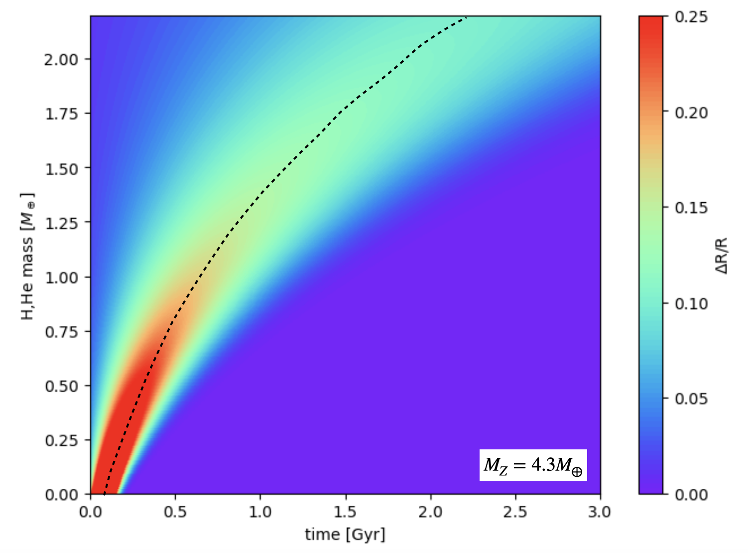
We then use equations 17 and 18 to obtain the maximum normalized radius inflation as a function of envelope mass in time (age). The radius inflation difference between a raining-out planet (R) and a core-envelope planet (RCE) with same composition () is time dependent. For the time dependency we fit the simulation results with a Gaussian, in which the standard deviation is the inverse of maximum radius inflation, and the mean is the rainout timescale. The results (/R) for planets with 4.3of silicates are presented in figure 8. As is shown, radius inflation is larger and earlier for planets with lighter envelopes.
3.5 Gas escape enhancement by rainout: Sedimentation-powered mass loss
In the case of a static (non-evolving) interior, the polluted envelopes may diminish mass loss by photoevaporation, due to higher envelope density and smaller radius. However, in an evolving interior the energy release by the rainout processes enhances mass loss, due to radius inflation. Mass-loss by photoevaporation is usually modeled by the energy-limited approach (e.g. Lammer et al., 2003; Owen & Wu, 2013; Lopez & Fortney, 2013), where planetary evaporation depends on the radius to the third power. From Rogers & Owen (2021):
| (19) |
where is efficiency coefficient, depending on the the escape velocity (), and XUV luminosity from a Sun-like star is
| (20) |
According to the equations above, larger radius, as a result of radius inflation by rainout, is expected to significantly increase mass loss rate, especially when the inflation takes place early on. But the other way around also holds: the loss of hydrogen from the surface of planets with polluted envelopes accelerates rainout via two channels - it raises the silicate to gas ratio in the outer envelope thus increasing oversaturation, and it removes part of the gas ”blanket” thus hasten the cooling. Therefore, if rainout timescale overlaps with the period of strong stellar XUV radiation the mass loss by photoevaporation, which is proportional to radius cube (eq. 19) grows significantly, boosting more radius inflation, which in turn enhances mass loss. Consequently, close-in and less massive planets with polluted envelopes are more vulnerable to enhanced mass loss by photoevaporation.
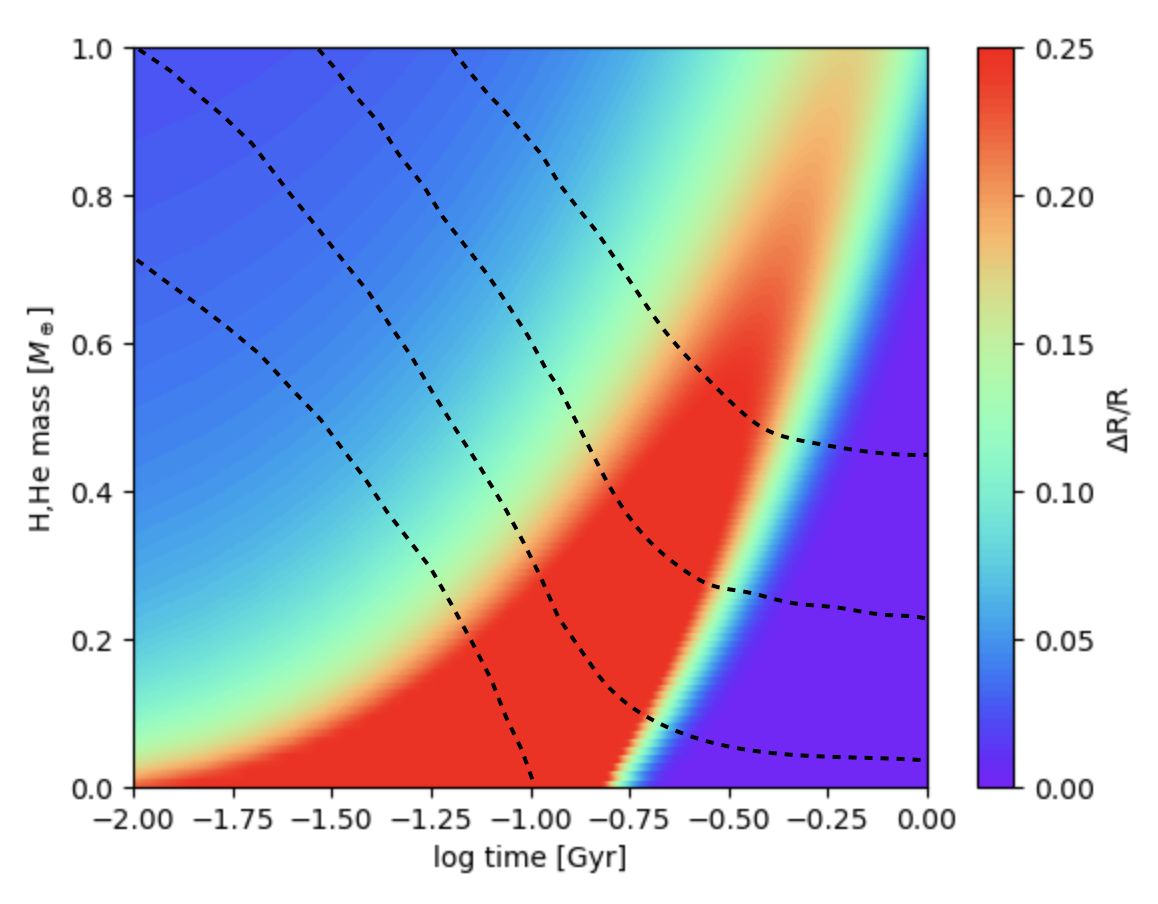
Figure 9 is a zoom-in of the first 1 Gyr of figure 8 in log time (x-axis). As can be seen, super-Earth planets with envelope masses below 0.4experience a major envelope expansion by rainout during the first hundreds of Myrs. This is when XUV-driven photoevaporation rates peak, then enhanced by ”sedimentation-powered” mass loss. Radius inflation of raining polluted envelopes that is larger by 0.25 () doubles the mass loss rate, and larger radius inflation of is translated to eight times more mass loss in comparison to a similar planet with initial core-envelope structure. The enhanced ”sedimentation-powered” mass loss, caused by the mutual effects of mass loss and rainout, may end in a complete strip of the gas envelope in planets that were born with polluted low-mass envelopes. A further investigation would require coupling the two processes to examine the mutual effect in detail.
3.6 Model parameter dependency
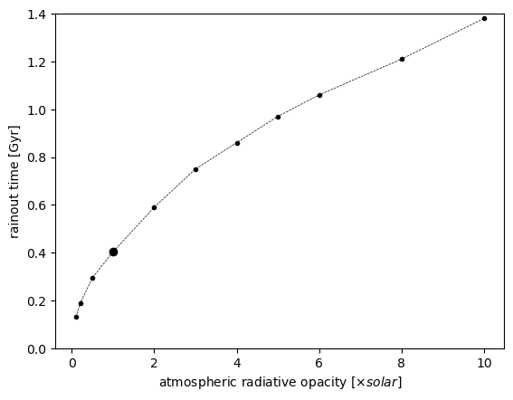
Atmospheric metallicity has a major role in cooling of gaseous envelopes, by changing the radiative opacity in the outer envelope, acting as the bottleneck for the planet cooling. Consequently, it influences the silicate rainout timescale. The higher the atmospheric opacity the longer the rainout time. Opacity can be affected by atmospheric phenomena like cloud formation or haze formation (Ormel & Min, 2019; Poser & Redmer, 2024). To explore the dependence of the atmospheric opacity on our results, we modify the outer atmospheric radiative metallicity. Specifically, we obtain the radiative opacity change by adjusting the parameter in equation 4 to values between 0.1-10 times solar. As is shown in figure 10, changing the atmosphere metallicity by two orders of magnitude (between 0.1-10 times solar) changes the rainout time by an order of magnitude. We remark that, although we have formulated the opacity in terms of a metallicity , adjusting the opacity by changing the value of has no bearing on the actual metallicity (composition) and overall equation of state. In this way, adjusting will directly inform us how the opacity affects the rainout timescale.
The effect of distance from the star on the results is not very strong and varies with mass. In massive planets and/or massive envelopes the distance from the parent star has negligible effect on an interior evolution and on the rainout process, as compressed gas density is determined mainly by gravity. In planets with light envelopes the irradiation effect can be noticeable. We find that the 5planet shown in figure 5 experiences 10% shorter rainout phase at 1 AU than at 0.2 AU. This comparison is for the same planetary mass and composition. Indirect effect of irradiation via mass loss is ignored in this comparison (see section 3.5 for mass loss effects).
We next examine the effect of planet formation conditions, such as pebble accretion rate and pebble size on the results. Planet formation conditions shape the initial temperature profile and metal distribution, yet varying the formation parameters within the range of Ormel et al. (2021) model has only small effect on the long term evolution. The reason is that planet formation parameters, unlike opacity and distance from the star, don’t influence the long-term cooling rate very much.
3.7 Overview and implications on observation interpretation
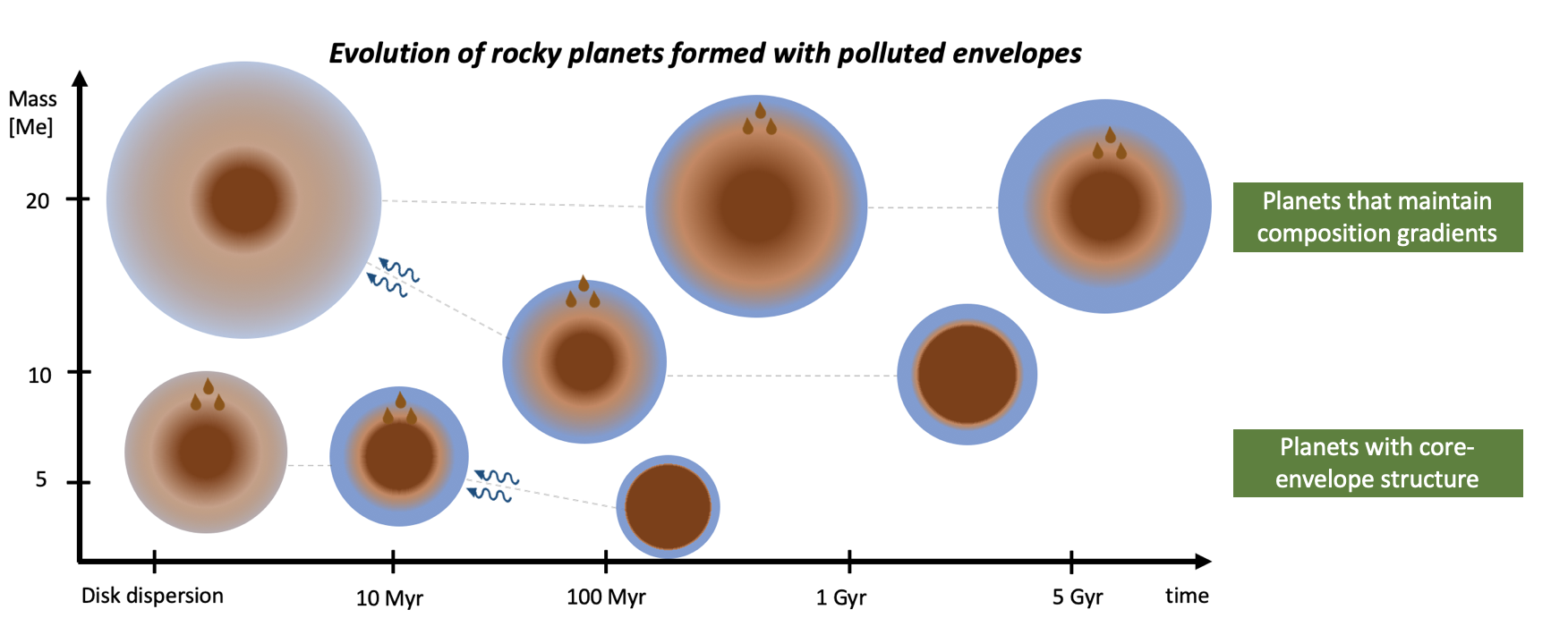
Our results indicate that rocky super-Earth-to-Neptune mass exoplanets can be classified into three groups regarding their interior structures, depending mainly on their mass and in particular their gas (H,He) mass:
-
1.
Planets that have lost their H,He envelope due to ”sedimentation-powered” mass loss and/or other mass loss mechanisms;
-
2.
Planets that retain a few percent of gas (by mass) after the mass-loss stage, whose interiors have since evolved to a core-envelope structure;
-
3.
Planets with thick envelopes that still have their interiors characterized by a composition gradient(s).
In figure 11 we show a schematic picture of the thermal and structural evolution of the planets that retain (part of) their primordial envelopes. The time and mass axes are for our standard set of parameters, and can vary with parameters as described in section 3.6.
The evolution of planets with polluted envelopes and the subsequent radius inflation by the rainout provides an alternative for the interpretation of planets’ radius-mass relation. The observed mass-radius relation if the planet is raining-out is overestimated in the standard model (see Vazan & Ormel 2023 for exoplanet examples). The main parameter to determine whether rainout takes place in an observed planet is its age. Although currently many of the observed planets don’t have good age estimates, in a few years a much larger and precise database of stellar ages will be available due to the PLATO mission (Rauer et al., 2014), which will allow us to examine the temporal dimension of the mass-radius relationship.
The heat flux generated by the interior of a planet experiencing rainout is significantly larger than in the standard (non-polluted) case, due to the release of rainout energy (potential energy, latent heat and formation energy). Certain chemical abundances, like the C/H ratio in the visible atmosphere of a planet may provide clues about the cooling history of the planet and its effective temperature (Fortney et al., 2020). Observations by JWST (Greene et al., 2016) and ARIEL (Tinetti et al., 2018) are expected to obtain spectra of a wide range of planetary atmospheres, and will help us identify those planets that formed with polluted envelopes.
The radius inflation caused by the rainout from polluted envelopes can explain, under certain conditions, the puffiness of observed close-in young planets, like the 0.5 Gyr old Kepler-51 system (Masuda, 2014; Libby-Roberts et al., 2020). In this scenario, mass loss and rainout mutual effect result in significant radius inflation that peaks at the observed age. The conditions to preform such evolutionary tracks require relatively high atmospheric metallicity and significant initial gas content. Moreover, if rainout is the dominant mechanism for puffing close-in young planets, then the current estimate of the gas content of these planets is an overestimate.
4 Discussion
The formation models of Ormel et al. (2021) stop at crossover mass, before the planet enters the runaway gas accretion phase. We show here that planets with massive envelopes (i.e., slow rainout) preserve their formation composition gradient. Massive (runaway) gas accretion on top of the planets we explore here would keep the deep interior undersaturated on timescales. This result is consistent with the indications of diluted core in Jupiter and Saturn (Vazan et al., 2016; Wahl et al., 2017; Debras & Chabrier, 2019; Mankovich & Fuller, 2021), and implies the Z-gradient may arise perhaps from formation, although other mechanisms can also redistribute the metals in the interior777In giant planets other processes such as miscibility of rock in metallic hydrogen (Wilson & Militzer, 2012; Soubiran et al., 2017, e.g.), and/or convective-mixing (Vazan et al., 2015; Müller et al., 2020) can change the long term interior structure..
We find that the envelope mass is the key factor that determines the timing and duration of the silicate rainout. However, initial envelope mass is an uncertain parameter, which varies with planet formation model assumptions. The initial envelope masses found in Ormel et al. (2021) are broadly within the range of other planet formation works (e.g., Mordasini, 2020; Lee & Chiang, 2015), but can vary with additional processes that potentially slow or halt gas accretion, like envelope recycling (Ormel et al., 2015; Kuwahara et al., 2019; Moldenhauer et al., 2021) that are not included in our formation model. Moreover, atmospheric boil-off (Owen & Wu, 2016; Rogers et al., 2023) can remove significant part of the envelope at very early evolution stage. We therefore vary the envelope masses resulting from the planet formation model, mainly to lower values than in the original model.
Although the work presented here assumes planets are formed by pebble accretion, some of the findings may also hold for planets formed by planetesimal accretion. Bodenheimer et al. (2018) and Valletta & Helled (2020) showed that formation of sub-Neptune planets by planetesimal accretion also terminates with a composition gradients, although steeper than in the pebble accretion case (Ormel et al., 2021). A further investigation is required to explore the silicate rainout processes in these planets.
4.1 Model limitations
The envelope metallicity follows the saturation L-V curve, in which silicate content increases with pressure and temperature, forming a composition gradient along the saturated envelope. For simplicity, we ignore the effect of this saturated outer composition gradient on the thermal evolution. Nevertheless, this additional composition gradient is expected to lead to convection inhibition and slow the cooling of the planet in this region (Guillot et al., 1995; Leconte et al., 2017). Markham et al. (2022) suggest this mechanism to lower the heat flux from deep interiors of sub-Neptunes, keeping the core in a high entropy supercritical state for billions of years, and permitting the dissolution of large quantities of hydrogen into the core. We anticipate this process to elongate the rainout timescales we find here, hence in this context our result provide a lower bound for the rainout timescale.
We use the liquid-vapor curve as a sole criterion for silicate redistribution, as in Podolak et al. (1988); Bodenheimer et al. (2018); Stevenson et al. (2022). We ignore in this work any chemical interaction between the silicates and the hydrogen. However, chemical interaction between species is expected to produce elements, like water and silane, that are not included in our study (Schaefer & Fegley, 2009; Misener et al., 2023; Horn et al., 2023). Dissociation of molecules in the deep interior, at temperature of about 5000 K and above (Melosh, 2007) is another mechanism that influence our results. Hydrogen dissolution in the rocky deep interior and out-gassing of the hydrogen as the planet cools (Chachan & Stevenson, 2018; Kite et al., 2019) may affect planets with low gas content.
We use the Freedman et al. (2014) radiative opacities as a function of pressure-temperature-metallicity. The original tables are valid in the range of up to 0.03 GPa in pressure, 4000 K in temperature, and 50X solar in metallicity. For higher values we extrapolated the radiative opacity, based on the analytical expressions provided in Freedman et al. (2014), as a function of pressure, temperature, and metallicity. The higher opacity obtained by the extrapolation leads to more convection in the outer composition gradient and upper envelope, thus, not necessarily slower cooling. Moreover, the radiative opacity effect is limited as the clean atmosphere (on top of the rainout boundary) is mainly convective, while the heat transport in the extrapolated high pressure layers (0.1 GPa), e.g., in the deep composition gradient is mainly conductive. We also note that the Freedman et al. (2014) opacity is calculated for solar ratio composition, in which contribution of species to the opacity is related to their solar abundances. Atmospheric metallicity that is based on L-V curves and cloud model (Poser & Redmer, 2024; Ormel & Min, 2019; Min et al., 2020) requires opacity calculation for other ratios, that may affect the rainout timescales we find here.
The planets we study in this work are rocky (dry) planets. Our results cannot be directly applied to planets containing large fraction of volatiles (wet planets) from two main reasons. First, volatile evaporate at the outer atmosphere and not in the deep interior, affecting the outer envelope properties and thus the planet formation and evolution process (Hori & Ikoma, 2011; Venturini et al., 2016; Kurosaki & Ikoma, 2017; Venturini et al., 2020). Second, perhaps more fundamentally to our work, miscibility of rock in water at high pressure (Nisr et al., 2020; Kim et al., 2021) may prohibit the silicate settling, leaving the rock mixed with the water on Gyr timescale (Vazan et al., 2022; Dorn & Lichtenberg, 2021). We therefore expect rainout and its consequent effects to be less remarkable in wet planets.
The thermodynamic properties of H,He are derived from the equation of state (EoS) of Saumon et al. (1995), for consistency with the planet formation calculation (Ormel et al., 2021). A newer EoS for hydrogen and helium mixture (Chabrier et al., 2019) indicate higher compressibility than Saumon et al. (1995) for density above 0.1 g/. Based on the results of Chabrier et al. (2019) we estimate a difference of up to 15% in envelope density-pressures relation for the planets in this work. Consequently, thermal evolution and rainout timescale are expected to be similar for the super-Earth planets in our sample, but longer for the more massive Neptune-like planets. Together with the convective-inhibition described above, the rainout timescales presented in this work are a lower bound.
5 Conclusions
By linking planet formation model to a non-adiabatic structure-evolution model, we have calculated the post-formation structure and thermal evolution of rocky planets formed by pebble accretion. Specifically, we have followed, for the first time, the fate of the hot silicate vapor that remained in the planet’s envelope after pebbles sublimated, as the planet cools. The model includes heat transport by radiation, convection and conduction, and mass redistribution by rainout (condensation and settling) and by convective-mixing. We find that the interior structure of silicate-rich planets that formed with polluted envelopes can be roughly divided in three groups, based on their envelope (H,He) mass: bare rocky cores that have lost their envelopes, super-Earth planets with core-envelope structure, and Neptune-like planets with diluted cores that are slowly raining-out. Our findings bridge the gap between the indications for composition gradients in massive planets (e.g., solar system gas giants) and core-envelope structure in small planets. Below are our main conclusions:
-
1.
Formation of sub-Neptune planets by pebble accretion (and to a lesser extent, planetesimal accretion) result in a strong composition gradient within the envelope, due to the thermal ablation of the pebbles (planetesimals). This composition gradient cannot be overturned by convection, but its metals can be redistributed due to rainout.
-
2.
Cooling of polluted envelopes leads to silicate rainout and late core growth. The interior structure of rocky sub-Neptunes is therefore determined by the time over which rainout proceeds (), which depends mainly on the envelope mass, but also on planet mass and atmospheric opacity. Specific formation conditions (e.g., the pebble size or the pebble accretion rate) are insignificant to the rainout process.
-
3.
The energy release that accompanies rainout – gravitational (settling) and to a lesser extent latent heat (condensation), as well as stored formation energy – act to inflate the planet radius, in comparison to a core-envelope analogue. Radius inflation is inversely proportional to the rainout timescale. Lower-mass planets have shorter rainout time and larger radius inflation. We provide an analytical estimate for the rainout timescale and radius inflation (section 2.3). Accurately age determinations are therefore key in order to properly interpret mass-radius relationships for planets with significant gas content.
-
4.
Young planets with envelopes lighter than 0.4experience their maximum radius inflation by rainout in the first hundreds of Myrs, during which they are prone to mass loss by photoevaporation. The mutually enforcing processes of radius inflation and mass loss in this period result in enhanced (sedimentation-powered) loss of envelopes for these planets.
-
5.
Planets with massive envelopes preserve their primordial composition gradients due to the blanketing effect of the envelope. Thus, Gyr old Neptune-like planets are expected to have gradual distribution of metals in their interiors.
Acknowledgments
We thank the referee for their constructive comments. We thank Tristan Guillot, Steve Markham, Masahiro Ikoma, Jonathan Fortney, and Re’em Sari for useful discussions. A.V. acknowledges support by ISF grants 770/21 and 773/21. C.W.O. acknowledge support by the National Natural Science Foundation of China (grant no. 12250610189 and no. 12233004). Figures were plotted using Matplotlib (Hunter, 2007).
Appendix A A comparison between ideal and non-ideal gas equations of state
A very common approximation in planet formation and evolution studies is that the gas is ideal. Its deviation from the more realistic EoS is usually not considered. One of the differences between our simulations and the analytical model in section 3.4 is the use of a tabular EoS in the simulations, while in the analytical calculation the gas is assumed ideal. To explore the difference we compare the ideal gas EoS against the tabular pressure-temperature-density relation of a H,He mixture. The ideal gas we used for the comparison is calculated for hydrogen and helium mass fraction of 0.7 and 0.3, respectively. The mean molecular weight of the H,He mixture is 2.35, the adiabatic index is 1.45 and the adiabatic gradient is 0.31, as in Ormel et al. (2021).
In figure 12 we plot the properties of the H,He mixture as a function of density and temperature, from the tabular EoS of Saumon et al. (1995). The H,He mixture is calculated according to the additive volume law, as in Vazan et al. (2013). Shown are the pressure normalized to the ideal gas pressure (top), and the related adiabatic temperature gradients (bottom). The upper panel of figure 12 indicates that gas density-pressure fairly agrees with ideal gas up to density of about 0.1 g/. The ideal gas pre-factor of 1/(2.35) is shown in red curve. At higher density the real gas diverges from the ideal gas, and is significantly less compressible than the ideal gas. Pressure-temperature profiles of the planets we modelled here indicate that most of the gas is at higher than 0.1 g/ density for most of the evolution time. In general, sub-Neptune planets with more than a few percent of gas have large fraction of their gas at high density, in which ideal gas assumption doesn’t hold. Consequently, modeling planets that have more than a few percent of gas by using ideal gas lead to unrealistically hotter envelopes and smaller radii.
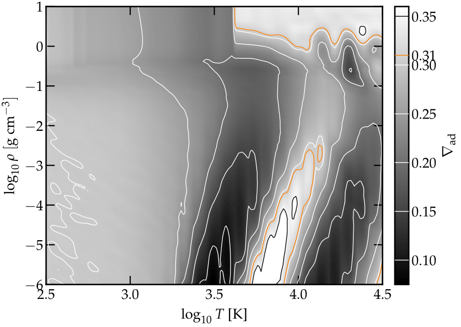
Another phenomenon that is ignored in ideal gas calculation is the ionization and dissociation of molecules, which affects the heat capacity and thus the temperature profile and evolution. In the bottom panel of figure 12 gray-scale represents the adiabatic temperature gradient (nabla) parameter, where ideal gas value is shown in orange curve. The ideal gas value of 0.31 (2/7 for H and 2/5 for He) is higher than of the real gas, for gas density above 0.1 g/, leading to too sharp temperature-pressure slope in models that are using ideal gas.
Appendix B Harmonic mean of radiative and conductive opacity
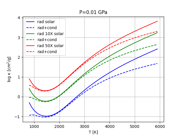
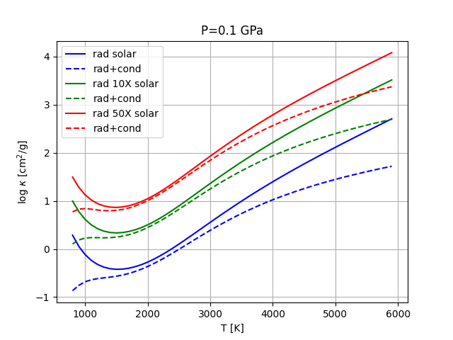
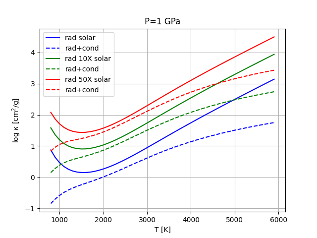
Conductive opacities are calculated from the thermal conductivity of silicate, as hydrogen-helium conductivity is negligible in the pressure-temperature range of interest (French et al., 2012). We take the thermal conductivity of Earth, (Stevenson et al., 1983) to be our reference values, and scale it with pressure and temperature according to Stamenković et al. (2011). Then, the harmonic mean of radiative and conductive opacities is calculated according to equation 3f. In figure 13 we present values of the radiative opacity (solid) and the harmonic mean of the radiative and conductive opacity (dashed) as a function of temperature, for three metallicity values (color) in three pressures (panels). Conduction scales linearly with the silicate mass fraction in a given layer. As can be seen, conduction dominates the heat transport as temperature and pressure increase.
References
- Baraffe et al. (2008) Baraffe, I., Chabrier, G., & Barman, T. 2008, A&A, 482, 315
- Bodenheimer et al. (2018) Bodenheimer, P., Stevenson, D. J., Lissauer, J. J., & D’Angelo, G. 2018, ApJ, 868, 138
- Brouwers & Ormel (2020) Brouwers, M. G. & Ormel, C. W. 2020, A&A, 634, A15
- Brouwers et al. (2021) Brouwers, M. G., Ormel, C. W., Bonsor, A., & Vazan, A. 2021, A&A, 653, A103
- Brouwers et al. (2018) Brouwers, M. G., Vazan, A., & Ormel, C. W. 2018, A&A, 611, A65
- Chabrier et al. (2019) Chabrier, G., Mazevet, S., & Soubiran, F. 2019, ApJ, 872, 51
- Chachan & Stevenson (2018) Chachan, Y. & Stevenson, D. J. 2018, ApJ, 854, 21
- Debras & Chabrier (2019) Debras, F. & Chabrier, G. 2019, ApJ, 872, 100
- Dorn & Lichtenberg (2021) Dorn, C. & Lichtenberg, T. 2021, ApJ, 922, L4
- Faik et al. (2018) Faik, S., Tauschwitz, A., & Iosilevskiy, I. 2018, Computer Physics Communications, 227, 117
- Fortney et al. (2013) Fortney, J. J., Mordasini, C., Nettelmann, N., et al. 2013, ApJ, 775, 80
- Fortney et al. (2020) Fortney, J. J., Visscher, C., Marley, M. S., et al. 2020, AJ, 160, 288
- Freedman et al. (2014) Freedman, R. S., Lustig-Yaeger, J., Fortney, J. J., et al. 2014, ApJS, 214, 25
- French et al. (2012) French, M., Becker, A., Lorenzen, W., et al. 2012, ApJS, 202, 5
- Ginzburg et al. (2016) Ginzburg, S., Schlichting, H. E., & Sari, R. 2016, ApJ, 825, 29
- Greene et al. (2016) Greene, T. P., Line, M. R., Montero, C., et al. 2016, ApJ, 817, 17
- Guillot (1995) Guillot, T. 1995, Science, 269, 1697
- Guillot (2010) Guillot, T. 2010, A&A, 520, A27
- Guillot et al. (1995) Guillot, T., Chabrier, G., Gautier, D., & Morel, P. 1995, ApJ, 450, 463
- Henyey et al. (1964) Henyey, L. G., Forbes, J. E., & Gould, N. L. 1964, ApJ, 139, 306
- Hori & Ikoma (2011) Hori, Y. & Ikoma, M. 2011, MNRAS, 416, 1419
- Horn et al. (2023) Horn, H. W., Prakapenka, V., Chariton, S., Speziale, S., & Shim, S. H. 2023, \psj, 4, 30
- Hunter (2007) Hunter, J. D. 2007, Computing in Science & Engineering, 9, 90
- Kaniel & Kovetz (1967) Kaniel, S. & Kovetz, A. 1967, Physics of Fluids, 10, 1186
- Kim et al. (2021) Kim, T., Chariton, S., Prakapenka, V., et al. 2021, Nature Astronomy, 5, 815
- Kippenhahn et al. (2013) Kippenhahn, R., Weigert, A., & Weiss, A. 2013, Stellar Structure and Evolution
- Kite et al. (2019) Kite, E. S., Fegley, Bruce, J., Schaefer, L., & Ford, E. B. 2019, ApJ, 887, L33
- Kovetz et al. (2009) Kovetz, A., Yaron, O., & Prialnik, D. 2009, MNRAS, 395, 1857
- Kraus et al. (2012) Kraus, R. G., Stewart, S. T., Swift, D. C., et al. 2012, Journal of Geophysical Research (Planets), 117, E09009
- Kurosaki & Ikoma (2017) Kurosaki, K. & Ikoma, M. 2017, AJ, 153, 260
- Kuwahara et al. (2019) Kuwahara, A., Kurokawa, H., & Ida, S. 2019, A&A, 623, A179
- Lammer et al. (2003) Lammer, H., Selsis, F., Ribas, I., et al. 2003, ApJ, 598, L121
- Leconte et al. (2017) Leconte, J., Selsis, F., Hersant, F., & Guillot, T. 2017, A&A, 598, A98
- Ledoux (1947) Ledoux, P. 1947, ApJ, 105, 305
- Lee & Chiang (2015) Lee, E. J. & Chiang, E. 2015, ApJ, 811, 41
- Libby-Roberts et al. (2020) Libby-Roberts, J. E., Berta-Thompson, Z. K., Désert, J.-M., et al. 2020, AJ, 159, 57
- Lopez & Fortney (2013) Lopez, E. D. & Fortney, J. J. 2013, ApJ, 776, 2
- Lopez & Fortney (2014) Lopez, E. D. & Fortney, J. J. 2014, ApJ, 792, 1
- Mankovich & Fuller (2021) Mankovich, C. R. & Fuller, J. 2021, Nature Astronomy, 5, 1103
- Markham et al. (2022) Markham, S., Guillot, T., & Stevenson, D. 2022, A&A, 665, A12
- Masuda (2014) Masuda, K. 2014, ApJ, 783, 53
- Melosh (2007) Melosh, H. J. 2007, Meteoritics and Planetary Science, 42, 2079
- Mihalas (1978) Mihalas, D. 1978, Stellar atmospheres, 2nd edition (W. H. Freeman and Co. San Francisco)
- Min et al. (2020) Min, M., Ormel, C. W., Chubb, K., Helling, C., & Kawashima, Y. 2020, A&A, 642, A28
- Misener & Schlichting (2022) Misener, W. & Schlichting, H. E. 2022, MNRAS, 514, 6025
- Misener et al. (2023) Misener, W., Schlichting, H. E., & Young, E. D. 2023, MNRAS[arXiv:2303.09653]
- Moldenhauer et al. (2021) Moldenhauer, T. W., Kuiper, R., Kley, W., & Ormel, C. W. 2021, A&A, 646, L11
- Mordasini (2014) Mordasini, C. 2014, A&A, 572, A118
- Mordasini (2020) Mordasini, C. 2020, A&A, 638, A52
- Movshovitz et al. (2010) Movshovitz, N., Bodenheimer, P., Podolak, M., & Lissauer, J. J. 2010, Icarus, 209, 616
- Movshovitz & Podolak (2008) Movshovitz, N. & Podolak, M. 2008, Icarus, 194, 368
- Müller et al. (2020) Müller, S., Helled, R., & Cumming, A. 2020, A&A, 638, A121
- Nisr et al. (2020) Nisr, C., Chen, H., Leinenweber, K., et al. 2020, Proceedings of the National Academy of Science, 117, 9747
- Ormel (2014) Ormel, C. W. 2014, ApJ, 789, L18
- Ormel & Min (2019) Ormel, C. W. & Min, M. 2019, A&A, 622, A121
- Ormel et al. (2015) Ormel, C. W., Shi, J.-M., & Kuiper, R. 2015, MNRAS, 447, 3512
- Ormel et al. (2021) Ormel, C. W., Vazan, A., & Brouwers, M. G. 2021, A&A, 647, A175
- Owen & Wu (2013) Owen, J. E. & Wu, Y. 2013, ApJ, 775, 105
- Owen & Wu (2016) Owen, J. E. & Wu, Y. 2016, ApJ, 817, 107
- Podolak et al. (1988) Podolak, M., Pollack, J. B., & Reynolds, R. T. 1988, Icarus, 73, 163
- Poser & Redmer (2024) Poser, A. J. & Redmer, R. 2024, MNRAS[arXiv:2402.19466]
- Rauer et al. (2014) Rauer, H., Catala, C., Aerts, C., et al. 2014, Experimental Astronomy, 38, 249
- Rogers & Owen (2021) Rogers, J. G. & Owen, J. E. 2021, MNRAS, 503, 1526
- Rogers et al. (2023) Rogers, J. G., Owen, J. E., & Schlichting, H. E. 2023, arXiv e-prints, arXiv:2311.12295
- Rosenblum et al. (2011) Rosenblum, E., Garaud, P., Traxler, A., & Stellmach, S. 2011, ApJ, 731, 66
- Saumon et al. (1995) Saumon, D., Chabrier, G., & van Horn, H. M. 1995, ApJS, 99, 713
- Schaefer & Fegley (2009) Schaefer, L. & Fegley, B. 2009, ApJ, 703, L113
- Soubiran et al. (2017) Soubiran, F., Militzer, B., Driver, K. P., & Zhang, S. 2017, Physics of Plasmas, 24, 041401
- Stamenković et al. (2011) Stamenković, V., Breuer, D., & Spohn, T. 2011, Icarus, 216, 572
- Steinmeyer et al. (2023) Steinmeyer, M.-L., Woitke, P., & Johansen, A. 2023, A&A, 677, A181
- Stevenson et al. (2022) Stevenson, D. J., Bodenheimer, P., Lissauer, J. J., & D’Angelo, G. 2022, \psj, 3, 74
- Stevenson et al. (1983) Stevenson, D. J., Spohn, T., & Schubert, G. 1983, Icarus, 54, 466
- Tinetti et al. (2018) Tinetti, G., Drossart, P., Eccleston, P., et al. 2018, Experimental Astronomy, 46, 135
- Valletta & Helled (2019) Valletta, C. & Helled, R. 2019, ApJ, 871, 127
- Valletta & Helled (2020) Valletta, C. & Helled, R. 2020, ApJ, 900, 133
- Vazan et al. (2015) Vazan, A., Helled, R., Kovetz, A., & Podolak, M. 2015, ApJ, 803, 32
- Vazan et al. (2016) Vazan, A., Helled, R., Podolak, M., & Kovetz, A. 2016, ApJ, 829, 118
- Vazan et al. (2013) Vazan, A., Kovetz, A., Podolak, M., & Helled, R. 2013, MNRAS, 434, 3283
- Vazan & Ormel (2023) Vazan, A. & Ormel, C. W. 2023, A&A, 676, L8
- Vazan et al. (2018a) Vazan, A., Ormel, C. W., & Dominik, C. 2018a, A&A, 610, L1
- Vazan et al. (2018b) Vazan, A., Ormel, C. W., Noack, L., & Dominik, C. 2018b, ApJ, 869, 163
- Vazan et al. (2022) Vazan, A., Sari, R., & Kessel, R. 2022, ApJ, 926, 150
- Venturini et al. (2016) Venturini, J., Alibert, Y., & Benz, W. 2016, A&A, 596, A90
- Venturini et al. (2020) Venturini, J., Guilera, O. M., Haldemann, J., Ronco, M. P., & Mordasini, C. 2020, A&A, 643, L1
- Wahl et al. (2017) Wahl, S. M., Hubbard, W. B., Militzer, B., et al. 2017, Geochim. Res. Lett., 44, 4649
- Wilson & Militzer (2012) Wilson, H. F. & Militzer, B. 2012, Physical Review Letters, 108, 111101