Quantum Metrology with Higher-order Exceptional Points in Atom-cavity Magnonics
Minwei Shi1Guzhi Bao1,2guzhibao@sjtu.edu.cnJinxian Guo1,2jxguo@sjtu.edu.cnWeiping Zhang1,2,3,4wpz@sjtu.edu.cn1 School of Physics and Astronomy, and Tsung-Dao Lee Institute, Shanghai Jiao Tong University, Shanghai, 200240, China
2 Shanghai Research Center for Quantum Sciences, Shanghai, 201315, China
3 Shanghai Branch, Hefei National Laboratory, Shanghai, 201315, China
4 Collaborative Innovation Center of Extreme Optics, Shanxi University, Taiyuan, 030006, China
Abstract
Exceptional points (EPs), early arising from non-Hermitian physics, significantly amplify the system’s response to minor perturbations,
and act as a useful concept to enhance measurement in metrology. In particular, such a metrological enhancement grows dramatically with the EP’s order.
However, the Langevin noises intrinsically existing in the non-Hermitian systems diminish this enhancement.
In this study, we propose a protocol for quantum metrology with the construction of higher-order EPs (HOEPs) in atom-cavity system through Hermitian magnon-photon interaction.
The construction of HOEPs utilizes the atom-cavity non-Hermitian-like dynamical behavior but avoids the external Langevin noises via the Hermitian interaction.
A general analysis is exhibited for the construction of arbitrary -th order EP (EPn).
As a demonstration of the superiority of these HOEPs in quantum metrology, we work out an EP3/4-based atomic sensor with sensitivity being orders of magnitude higher than that achievable in an EP2-based one.
We further unveil the mechanism behind the sensitivity enhancement from HOEPs.
The experimental establishment for this proposal is suggested with potential candidates.
This EP-based atomic sensor, taking advantage of the atom-light interface, offers new insight into quantum metrology with HOEPs.
††preprint: APS/123-QED
Introduction.–
In the past decades, new approaches for precision measurement have been proposed based on exceptional points (EPs), where the -th order EP (EPn) indicates the coalescence of the system’s () eigenvalues and their corresponding eigenstates Miri and Alu (2019); Heiss (2012); Özdemir et al. (2019); Peng et al. (2016); Liang et al. (2023).
The system exhibits a nonlinear response to external perturbations near EPn, with the response scaling as for Chen et al. (2017); Wiersig (2016, 2020); Zhang et al. (2019); Wiersig (2014); Hokmabadi et al. (2019); Mao et al. (2023); Zhong et al. (2020); Mandal and Bergholtz (2021); Sayyad and Kunst (2022).
This power-law behavior, increasing dramatically with EPs’ order , highlights the system’s advantage as sensors based on higher-order EPs (HOEPs) in metrology Hodaei et al. (2017); Zeng et al. (2019); Wu et al. (2021); Xiao et al. (2019).
Despite the promise of EPs, the presence of intrinsic Langevin noise in non-Hermitian systems poses an obstacle to the sensitivity enhancements Wang et al. (2020); Langbein (2018); Chen et al. (2019); Duggan et al. (2022); Anderson et al. (2023); Ding et al. (2023).
To solve this issue, several strategies have been proposed, including the use of post-selection techniques to discard quantum noise Naghiloo et al. (2019), and Hamiltonian dilation by integrating the non-Hermitian system and the reservoir as a large Hermitian system Wu et al. (2019); Sergeev et al. (2023).
Recent demonstrations have shown that EPs can also be constructed within Hermitian systems that include nonlinear coupling Wang and Clerk (2019); Jiang et al. (2019); Luo et al. (2022).
In such systems, the EPs delineate the dynamical phase transition between parametric oscillation and parametric amplification.
For a quadratic bosonic system with Hamiltonian:
(1)
EPs appear at the parametric amplification threshold of the system where the bilinear coupling strengths reach a certain equilibrium with the detunings and the linear coupling strengths .
These EPs emerge solely from the system’s non-Hermitian-like behaviors, rather than from losses and gains, and are therefore not subject to Langevin noise limitations.
In this paper, we propose a novel cavity-mediated atomic sensor that utilizes HOEPs with nonlinear responses to external perturbations while immunizing Langevin noise.
The cavity mode interacts with the collective spin-wave excitations (magnons) though either SU(1,1)- or SU(2)-type Raman interaction Chen et al. (2009); Hammerer et al. (2010); Chen et al. (2010, 2015); Guo et al. (2019); Wen et al. (2019), and establishes couplings among multiple atomic ensembles to form HOEPs.
The HOEPs enhance the sensing capability of atoms, resulting in an outstanding performance for sensitivity of probing various fields in demand, such as electric fields Khadjavi et al. (1968), magnetic fields Budker and Romalis (2007), optical fields Delone and Krainov (1999), and even exotic fields Pustelny et al. (2013).
The main aspects of our work include:
(i) Despite the Hermiticity of magnon-photon interaction in our model, the system’s dynamical matrix exhibits non-Hermiticity, and satisfies both pseudo-Hermiticity (psH) Mostafazadeh (2010); Mostafazadeh and Batal (2004); Mostafazadeh (2002) and particle-hole symmetry (PHS) Delplace et al. (2021); Sayyad and Kunst (2022); Okugawa and Yokoyama (2019).
By tuning the interaction strengths and detunings, we identify the emergence of HOEPs from spontaneous breaking of these symmetries.
(ii)
We further provide the necessary condition for the system to attain EP with highest order allowed in the system: the entire atom-cavity system must be irreducible. The system’s irreducibility can be determined by the Casimir invariants of the SU(1,1) and SU(2) transformations Yurke et al. (1986); Ban (1993).
(iii)
As an illustration, we devise an EP3-based atomic sensor employing homodyne detection, showing sensitivity orders of magnitude superior to EP2-based one. This sensitivity enhancement is solely arising from HOEPs instead of quantum squeezing.
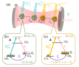
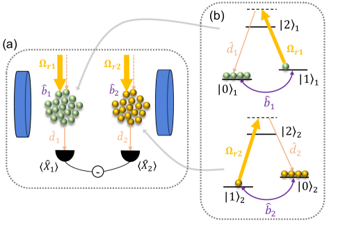
Figure 1: (a) Atom-cavity system to realize EPn. atomic ensembles are placed inside a cavity, where () ensembles interact with the cavity mode through SU(1,1)-type Raman interactions (b), and the remaining ensembles interact with the cavity mode through SU(2)-type Raman interactions (c). (b) and (c) depict the atomic energy levels and mechanisms of the SU(1,1)- and SU(2)-type atom-light interactions, respectively.
The Model.– The proposed atom-cavity system is illustrated in Fig. 1 (a-c).
Each atomic ensemble consists of atoms with a pair of lower metastable states and , as well as an excited state .
Here labels a particular atomic ensemble. Coherence between the states and can be established and represented by the atomic spin wave .
Using the Holstein-Primakoff transformation Holstein and Primakoff (1940) and assuming that the mean number of atoms transferred to the state is much smaller than , we can view the collective spin-wave excitations in the atomic ensembles as quasiparticles known as magnons and express it in terms of bosonic annihilation operator , i.e. .
Our system exploits two types of Raman interactions between the cavity field and the magnon fields: SU(1,1)- and SU(2)-type Chen et al. (2009); Hammerer et al. (2010); Chen et al. (2010, 2015); Guo et al. (2019); Wen et al. (2019).
For convenience, we assume that the first atomic ensembles interact with the cavity mode via SU(1,1)-type Raman interactions.
They are initially prepared though optical pumping in state with , as shown in Fig. 1 (b).
Pump light couples the state and the excited state with a large single-photon detuning to simultaneously generate correlated magnon field and cavity field .
By adiabatically eliminating the excited state , we have the Hamiltonian that obeys the Lie algebra of SU(1,1).
The remaining atomic ensembles experience the SU(2)-type Raman interactions.
They are initially prepared though optical pumping in another metastable state, here for convenience, relabelled as with in our theoretical treatment, as shown in Fig. 1 (c).
The magnon field interchanges with the cavity field via pump light detuned by . By performing adiabatically elimination of , we end at Hamiltonian that obeys the Lie algebra of SU(2).
The Hamiltonian of the whole system is then given by:
(2)
Here , is the two-photon detuning and represents the external perturbation acting on the particular magnon mode . and are the effective coupling coefficients of SU(1,1)- and SU(2)-type Raman interaction, respectively. and represent the atomic transition coefficients.
We utilize such an atom-cavity system as a quantum sensor to detect the external perturbations .
In the following context, we set all atomic ensembles to experience the same perturbation on the detuning , The result of is shown in [SuppMatt S1 and S3].
Emergence of higher-order exceptional point.–
Despite the Hermiticity of the system’s Hamiltonian, non-conservative SU(1,1) terms lead to a non-Hermitian-like dynamics of system.
We can formulate the system’s dynamics based on the Heisenberg equation:
(3)
Here is the field vector and is the non-Hermitian dynamical matrix of our system.
inherently follows the PHS, i.e. with ; as well as the psH, i.e. with . Here, is the identity matrix and are the Pauli matrices. The spontaneous breaking of these symmetries induces a dynamical phase transition, leading to the emergence of EPs of at least order two.
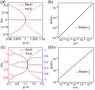
Figure 2: EP3 and EP4 realized in Hermitian atom-cavity system. (a) The eigenvalues of . Red solid (blue dashed) lines represent the real (imaginary) parts. Parameters used are . (b) Logarithmic scale plot of the absolute eigenvalue splitting at EP3 () as a function of perturbation with slope=1/3, showing the cubic-root response. (c) The eigenvalues of . Parameters used are , , and . (d) Logarithmic scale plot of the absolute eigenvalue splitting at EP4 () as a function of perturbation with slope=1/4, showing the biquadratic-root response.
Achieving the highest-order EPn in our system necessitates that the dynamical matrix be irreducible, indicating that the system cannot be decomposed into independent subsystems under linear transformations.
This can be identified through the Casimir invariants of SU(2) and SU(1,1) transformations.
For subsystems composed of two magnon modes ( and ) engaging in different types of interactions with the cavity mode, the system’s irreducibility requires that their free-field Hamiltonian not be proportional to the SU(1,1) invariant , i.e., .
Otherwise, for , the whole system is reducible: there exists a suitable SU(1,1) transformation to reduce the number of effective magnon modes interacting with the cavity mode.
On the other hand, for subsystems composed of two magnon modes engaging in the same type of interactions, we require its free-field Hamiltonian not be proportional to the SU(2) invariant , i.e., .
Similar to the above case, if this condition is not satisfied, the system can be reduced by performing a suitable SU(2) transformation.
Generally, to achieve an EPn in a system with atomic ensembles, the two-photon detunings adhere to the condition where .
To better understand the necessary conditions provided above, we present a counterexample in a system with two atomic ensembles. The two magnon modes interact with the cavity field through SU(1,1) and SU(2) interactions, respectively.
The dynamical matrix is as follows:
(4)
In principle, this system can achieve EP3 which is the highest order of EP allowed in the system with two atomic ensembles.
However, if (), we can perform an SU(1,1) transformation to introduce two new effective magnon modes:
(5)
that guarantees the particle number difference being invariant.
With these new modes, the Hamiltonian of the interaction reduces to with only one effective magnon mode interacting with the cavity field.
The eigenvalues of the system then become , which only exhibits EP2.
For and which satisfies the necessary condition of system’s irreducibility, system exhibits EP3, as shown in Fig. 2 (a-b).
At this EP3, the system’s eigenvalues exhibit cubic-root responses to perturbations in two-photon detuning [SuppMatt S1].
Further extending this system by adding an atomic ensemble undergoing an SU(1,1)-type interaction with the cavity mode elevates the order of EP to four.
As shown in Fig. 2 (c-d), EP4 is achieved in this system when .
At this EP4, the system’s eigenvalues exhibit biquadratic-root responses to the perturbations in two-photon detuning.
EP3-based sensor.–
The higher-order response of the eigenvalues at the HOEP suggests dramatic changes in systemic dynamics, indicating enhanced performance of the HOEP-based sensor.
To clearly demonstrate the contribution of HOEPs in Hermitian system to the sensitivity of sensors, we develop and evaluate an atomic sensor based on EP3 in the system described by Eq. 4.
The system’s dynamics on both sides of EP3 exhibits different behaviors: parametric oscillation when and parametric amplification when .
For the parametric-amplification phase, atomic excitation grows exponentially with time, and induces extra higher-order nonlinear effects (such as ). These nonlinear effects become significant and can no longer be neglected in Eq. 2 for long-time scenario, destroying the non-Hermitian symmetry of the dynamical matrix.
Therefore, we focus on the EP3-based sensor in the parametric-oscillation phase to build a stable sensing system.
For a perfect optical cavity, the time evolution of the magnons can be obtained from Eq. 3 and Eq. 4:
(6)
(7)
Here, are the propagation coefficients depending on which determine the evolution of magnons, as given explicitly in the [SuppMatt S2 and S3] (including both the exact solutions and the first order perturbation approximations).
We can observe the changes of the system caused by external perturbations though performing homodyne measurements on magnon modes, thereby estimating the perturbations.
This measurement strategy is implemented by leveraging another SU(2)-type Raman interaction to read out the magnon modes. This interaction fully converts magnon modes into photons, which is then detected by standard homodyne measurements [SuppMatt S4].
We consider a coherent initial state for magnon modes .
Without loss of generality, we set with a real and in the following context.
We select the observable (see details in [SuppMatt S3] ) to reflect the system’s change.
Here, is the quadrature operator of the particular magnon mode .
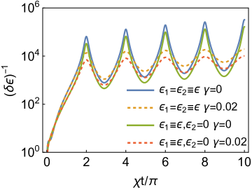
This change is quantified by the susceptibility , which is maximized near , as shown in Fig. 3 (a).
From the first order perturbation theory [SuppMatt S3], we have the susceptibility at :
(8)
where and .
The local maxima can be reached at the working point with , see Fig. 3 (b-c).
Near EP3 (), the susceptibility exhibits a divergent feature, induced by EP and representing EP-enhanced response to perturbations.
The noise of this sensor can be expressed as the variance of the observable .
As shown by the red curves in Fig. 3 (b), the local minima of noise is reached at the time . In such a case, the system evolves back to its initial coherent state.
Thus at the working point , the optimal sensitivity of the system is .
During the evolution, the number of atomic excitations is and the time for reaching the working point is .
Therefore, the optimal sensitivity scales at Heisenberg limit .
Notice that, entanglement can be achieved between two atomic ensembles Parkins et al. (2006); Dalla Torre et al. (2013) which contributes the anti-squeezing feature of the observable .
In particular, for , the noise reaches its maximum and the sensitivity reaches worst as .
The only reason for the Heisenberg scaling sensitivity of our sensor is from the HOEP enhancement instead of quantum entanglement/squeezing.
Figure 3: (a) The mean value of observable varying with perturbation at different working points. The shaded areas represent the measurement variance. (b) The variance (red) and susceptibility (blue) of observable as a function of evolution time when . (c) The reciprocal of sensitivity as a function of evolution time when . The solid blue (orange dot-dashed) curve shows the result of numerical simulation (first-order perturbation theory). In (b) and (c), the dashed curves represent the imperfect cavity case (). In all plots, we set , , and .
The impact of cavity loss (denoted by cavity decay rate ) is also examined [SuppMatt S3], as shown by the dashed lines in Fig. 3 (b-c).
The cavity’s loss causes the system to undergo damped oscillation in both susceptibility and noise .
In the long-time limit , the SU(1,1)-type Raman interaction in the system amplifies the vacuum noise introduced by cavity imperfection, leading to a constant noise that diminishes the EP-induced enhancement.
For the lossy cavity, the first working point becomes a better choice.
Higher-order EP enhancement.–
For comparison, we consider a quantum sensor based on Langevin noise-free EP2 Luo et al. (2022), with its optimal sensitivity scales at . This is evidently lower than that of our EP3-based sensor (scales at ), though both of them scale at Heisenberg limit .
We further notice that for an EPn-based atomic sensor operating in the parametric-oscillation phase, there exists a general scaling law for its sensitivity similar to .
This is attributed to the higher amplification rate of atomic (bosonic) excitations near HOEP, enhancing the sensitivity [SuppMatt S5].
Experimental realization.–
For an experimental setup with achievable parameters, we consider atoms with the states and corresponding to , and corresponding to . An external field is applied to lift the degeneracy of the states and enable distinct Raman transition channels between these states. The transitions to are coupled using circularly polarized pump and cavity fields, respectively.
To implement SU(1,1)- and SU(2)-type interactions, the atomic ensembles are initially prepared in different states via separate optical pumping.
We assume the initial magnon modes are prepared in coherent states with .
We select atomic transition coefficients and detuning . With pump beams of approximately and waists around , the resulting Rabi frequencies are .
This setup yields magnon-photon interaction strengths of .
Focusing on the EP3-based sensor, we can fine-tune and by adjusting the intensity of the pump light. Within the allowed precision of adjustment, is achievable, corresponding to .
Given these parameters, this atom-based sensor is capable of detecting perturbations , with sensitivity , corresponding to, e.g., a sensitivity for magnetic field measurement at the working point .
Conclusion.–
In summary, we develop an atom-cavity sensor that allows Langevin noise-free HOEPs to achieve high sensitivity.
Notably, this sensor demonstrates a sensitivity far surpassing that of EP2-based sensors.
Due to the versatility of atoms, the external perturbation can be induced by different interactions of atoms with various measured fields, including the Stark effect from electric fields Khadjavi et al. (1968), the Zeeman effect from magnetic fields Budker and Romalis (2007), the AC Stark effect from optical fields Delone and Krainov (1999), and even exotic interactions from axion-like particles Pustelny et al. (2013).
The crucial contribution of Langevin noise-free HOEPs in enhancing the atom-cavity system’s response to various measured fields represents a significant advance in precision measurement, indicating a new direction in sensing with quantum technology.
This work is supported by the Innovation Program for Quantum Science and Technology (2021ZD03032001); the National Natural Science Foundation of China (12234014, 11654005, 12204303, 11904227, 12374331); the Shanghai Municipal Science and Technology Major Project (2019SHZDZX01); the National Key Research and Development Program of China (Grant No. 2016YFA0302001); W. Z. also acknowledges additional support from the Shanghai talent program.
Hodaei et al. (2017)H. Hodaei, A. U. Hassan,
S. Wittek, H. Garcia-Gracia, R. El-Ganainy, D. N. Christodoulides, and M. Khajavikhan, Nature 548, 187 (2017).
Pustelny et al. (2013)S. Pustelny, D. F. Jackson Kimball, C. Pankow, M. P. Ledbetter, P. Wlodarczyk, P. Wcislo,
M. Pospelov, J. R. Smith, J. Read, W. Gawlik, et al., Annalen der Physik 525, 659 (2013).
In this supplementary material, we provide detailed descriptions of the system’s eigenvalues, evolution, first order perturbation approximation, the magnon modes read-out process, and the sensitivity scaling of EPn-based sensor, to support the results presented in the main text.
Appendix A S1. Third and fourth-order exceptional point
In order to solve the eigenvalues of the system’s dynamical matrix and systemic dynamics, we only need to consider half of the field operators in the field operator vector in the main text, as the other half are the Hermitian conjugates of this half.
We choose the field operator () for the atomic ensembles undergoing SU(1,1)-type interaction, () for the atomic ensembles undergoing SU(2)-type interaction, and the cavity field operator to form the shortened -dimensional field vector .
The Heisenberg equation of motion derived from this shortened field vector can fully describe the dynamical behavior of the system.
The corresponding simplified dynamical matrix is then given by
(S1)
with .
In the following context, we use this shortened field vector and simplified dynamical matrix to calculate the eigenvalues and the system’s dynamics for convenience.
A.1 A. EP3 in 3-mode system for one SU(1,1) and one SU(2) case
In this subsection, we calculate the solution of eigenvalues of a 3-mode system that is comprised of two atomic ensembles and one cavity mode. The cavity mode interacts with one of these two atomic ensembles through SU(1,1)-type Raman interaction, while interacting with the other one through SU(2)-type Raman interaction.
The corresponding simplified dynamical matrix for this system is:
(S2)
Here, we set and for convenience.
The diagonalization of can be done by the Cardano’s method kurosh1972higher. Its characteristic equation is given by:
(S3)
The solution is:
(S4)
(S5)
(S6)
where with
(S7)
(S8)
The expression is called the discriminant of the eigenvalue equation. If , then one of eigenvalues is real and other two are complex conjugate . In this case, the system is unstable and goes divergent in long time limit. If , then all eigenvalues are real and unequal, and the system is dynamically stable. The exceptional points (EPs) appear when , in which case, at least two eigenvalues are equal. In particular, when , all three eigenvalues coalesce with each other to form a third-order EP (EP3).
We focus on finding EP3 in the absence of external perturbation ().
When and , EP3 is achieved with degenerated eigenvalues and coalesced eigenvectors .
Next, we examine the splitting of eigenvalues at this EP3 under the external perturbations. We consider two cases: the same perturbation for both ensembles () and different perturbations for each ensemble ().
The same perturbations for both atomic ensembles :
In this case, we set . The equation S3 then reduces to
(S9)
which can be perturbatively expanded using Newton–Puiseux series Hodaei et al. (2017). For , we consider the first two terms only: , with the coefficients and being complex constants. Then equation S9 becomes
(S10)
Forcing the coefficients of first two terms to be zero, we obtain: and . Therefore we have the perturbed eigenvalues:
(S11)
(S12)
(S13)
Different perturbations for each atomic ensemble :
In order to exhibit the cubic-root response of EP3 in this case, we set for convenience. Again using Newton–Puiseux series, we have:
(S14)
Forcing the coefficients of first two terms to be zero, we obtain the solution: and . The corresponding eigenvalues are:
(S15)
(S16)
(S17)
It is obvious that in both situations, the eigenvalues response nonlinearly and scales at . When , there is a higher response with a factor of . This is attributed to the double signal acquisition in this case, while only one atomic ensemble senses the signal from external perturbation.
It is worth mention that in this case, if , equation S3 at EP3 becomes:
(S18)
which makes only linearly responds to the perturbation .
The reason is presented in the main text: the free-field Hamiltonian of magnon modes and is proportional to the Casimir invariant of the SU(1,1)-type interaction, i.e., .
A.2 B. EP4 in 4-mode system for two SU(1,1) and one SU(2) case
In this subsection, we derive the eigenvalues of a 4-mode system that is comprised with three atomic ensembles and one cavity mode. The cavity mode interacts with first two atomic ensembles through SU(1,1)-type Raman interaction, while interacting with the other one through SU(2)-type Raman interaction. The corresponding simplified dynamical matrix for this system is expressed by:
(S19)
Here, we set , and for convenience.
We focus on finding EP4 in this system in the absence of external perturbation ().
Then, the corresponding characteristic equation is:
(S20)
By converting the equation S20 into biquadratic form, we obtain the conditions for the system to have an EP4:
(S21)
(S22)
(S23)
with .
The eigenvalues are then expressed by:
(S24)
It is readily to find that EP4 is achieved when . At this EP4, and the system has only one coalesced eigenvector .
Similarly, the eigenvalues’ biquadratic-root response at EP4 can be examined by the Newton-Puiseux series.
This will not be reiterated here.
Appendix B S2. System evolution
In this section, we provide the solution of system’s dynamics in terms of the evolution matrix .
B.1 A. General solution of -mode system
By diagonalizing (equation S1), we obtain a series of eigenvectors () that is expressed by their corresponding eigenvalues :
(S25)
With these unnormalized eigenvectors , we can derive the evolution matrix , where is the unnormalized eigenvector matrix.
The matrix elements of represent the propagation coefficients of the system:
(S26)
(S27)
(S28)
where is the -th order polynomial for with .
B.2 B. Evolution matrix for 3-mode system described by
In this subsection, we derive the evolution matrix for a 3-mode system that is described by (equation S2).
In the main text, we approach the EP3 by adjusting , and observe the system’s response to external perturbations .
Therefore, we set , and formulate the evolution matrix as a function of and .
With the diagonalization of , we obtain the evolution matrix of the equation through its eigenvalues and eigenvectors, which is given by:
(S29)
Here, is the unnormalized eigenvector matrix:
(S30)
Solving equation S29 directly is difficult.
Fortunately, from the structure of equations S3-S6, we derive the following relationships between eigenvalues:
(S31)
Using these relations, we solve the evolution matrix:
(S32)
with propagation coefficients
(S33)
(S34)
(S35)
(S36)
(S37)
(S38)
Here, is the normalization factor and .
Appendix C S3. First order perturbation theory for EP3-based sensor
Differentiating the propagation coefficients in equation S33-S38 directly with respect to or is extremely difficult, preventing us from intuitively understanding the result. Therefore, in this section, we use first order perturbation theory to obtain an approximate solution for the systemic dynamics li2023speeding.
In non-Hermitian systems, the orthogonality of eigenvectors is disrupted, especially at the EPs, where two or more eigenvectors coalesce, leading to a reduction in the dimension of the Hilbert space . To address this issue, it is necessary to establish a biorthogonal eigenbasis on the dual Hilbert space . The results help us in performing the first order perturbation approximation.
To perform first order perturbation approximation near EP3, we firstly set and then construct the unperturbed biorthogonal eigenbasis as a function of .
In the following, we focus on the stable side of the system dynamics (). The reason is presented in the main text.
For convenience, we set .
C.1 A. Biorthogonal eigenbasis of unperturbed
In the absence of perturbation () but with the consideration of imperfect cavity (), the dynamical matrix reads
(S39)
with eigenvalues
(S40)
where . Their corresponding normalized right eigenvectors (i.e., ) are
(S41)
Note that in the case when and , three eigenvalues and eigenvectors coalesces with each other () which is the feature of EP3. These eigenvectors are not orthogonal:
(S42)
This is originated from the non-Hermiticity of .
We thus extend our eigenbasis to the state in the dual space , i.e., .
The corresponding normalized left eigenvectors are:
(S43)
Similarly, the left eigenvectors are also not orthogonal:
(S44)
Indeed, the right and left eigenvectors are non-orthogonal in their respective Hilbert spaces ( and ). They however form a biorthogonal eigenbasis in the Liouville space ():
(S45)
Therefore, we obtain the normalized biorthogonal eigenbasis and :
(S46)
and
(S47)
This biorthogonal eigenbasis also satisfies the normalization and completeness relations:
(S48)
C.2 B. First order perturbation approximation
In this section, we consider the case of existing small external perturbation (), and perform first order perturbation approximation to solve the perturbed system’s dynamics.
Given the perturbation Hamiltonian , we have the perturbation part of dynamical matrix
(S49)
The perturbation matrix in the space formed by right- and left-eigenvectors ( and ) is then expressed by:
(S50)
The perturbed eigenvalues are given by the diagonal terms in equation S50:
(S51)
(S52)
The corresponding perturbed right eigenvectors are given by
(S53)
(S54)
and the perturbed left eigenvectors are given by:
(S55)
(S56)
For the case of , we have
(S57)
(S58)
(S59)
Hence, these perturbed eigenvectors still satisfy the orthogonality, normalization, and completeness conditions.
C.3 C. State evolution
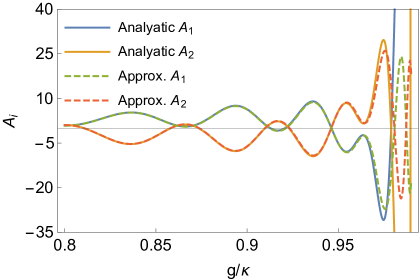
Figure S1: Propargating coefficients and versus for fixed time . The solid lines shows the numerical simulations of analytic results (equation S33-S38), and the dashed lines represent the results from first order perturbation theory (equation S61-S66). In this plot, we set the perturbation strength and .
Similar to equations S29 and S30, we define the perturbed system evolution matrix based on the perturbed biorthogonal eigenvectors
(S60)
For a perfect cavity (), we have the matrix elements as the propagation coefficients:
(S61)
(S62)
(S63)
(S64)
(S65)
(S66)
As shown in figure S1 and figure 3 in main text, as long as , the results of the first order approximation (equation S61-S66) agree well with the analytic results (equation S33-S38).
C.4 D. The selection of observable
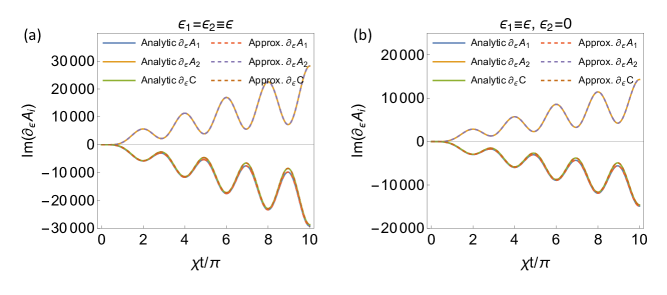
Figure S2: The time evolution of the derivative of propagation coefficents with respect to perturbation strength for (a) case and (b) case. The solid and dashed curves represent the results from the analytic solution and first order perturbation theory, respectively. In both plots, we set and .
In our EP3-based sensor, we initially prepare the magnon modes in atomic coherent states. At the working point, we perform the homodyne measurement on the read-out magnon modes. As can be seen from equation 6 and 7 in the main text, the measurement signal is proportional to the derivative of the propagation coefficient (i.e. and ) which can be calculated from equation S61-S66.
The same perturbations for both atomic ensembles (): The derivatives of and with respect to are given by:
(S67)
(S68)
(S69)
As shown in figure S2 (a), the derivative of has a different sign compared to the derivatives of and . Therefore, for the initial states where with real , we choose as the observable to maximize the susceptibility
(S70)
which scales at as given explicitly in equation 8 of the main text. The properties of noise and the sensitivity are elucidated in the main text.
Figure S3: The time evolution of the reciprocal of sensitivity for observable for (a) case and (b) case. The solid and dashed curves represent the results of perfect cavity () and imperfect cavity (), respectively. Here, we set and .
Different perturbations for each atomic ensemble (): In this case, the derivatives of and with respect to are given by:
(S71)
(S72)
(S73)
As shown in figure S2 (b) and figure S3, the results under this mode are very similar to those obtained with the case, and thus will not be elaborated upon here.
The difference lies in the smaller susceptibility and sensitivity.
The reason for this inferior performance is that only one atomic ensemble senses the signal of external perturbation in this case.
Appendix D S4. Magnon read-out process with SU(2)-type magnon-photon interaction
In this section, we use the EP3-based sensor as an example to demonstrate how magnons is converted into photons through SU(2)-type magnon-photon interaction.
At the working point , the interaction for sensing is stopped.
We can expand the state of two magnon modes and at the work point under the Fock basis:
(S74)
Here, means trace over mode and is the 3-mode magnon-photon hybrid state of the time.
Figure S4: (a) The schematic diagram of magnon read-out process and the homodyne detection on the read-out light mode. (b) The energy level of SU(2)-type Raman interaction for each atomic ensemble.
The reading process is achieved through the SU(2)-type Raman interaction, whose Hamiltonian is given by:
(S75)
where are the light modes for homodyne detections and initially prepared in vacuum states.
is the effective coupling coefficient. Here for convenience, we assume .
The evolution operator of this process is therefore .
After interaction time , the output state of two magnon and output light modes is given by:
(S76)
When , the state becomes
(S77)
Here, and which means both magnon modes are converted into photons and back to their vacuum states. Therefore, the homodyne measurements performed on the read-out light modes can fully extract the information carried by the atomic ensembles.
Appendix E S5. The scaling of sensitivity near -th order EP
In this section, we briefly analyze the scaling factor of the sensitivity with the perturbation (and the corresponding ) for our proposed EPn-based atom-cavity sensor.
Similar to the EP3-based sensor, we can obtain perturbation information by performing homodyne detection on the read-out magnon modes.
We consider the coherent initial state for the magnon modes. The susceptibility is then given by the derivative of the propagation coefficients with respect to :
When the system is at EPn () and exhibits an -th order response to the perturbation , the splitting corresponding to each eigenvalue is:
(S79)
with .
The denominator of is then .
We note that when , the polynomial can be regarded as a quantity independent of . When , since , the polynomial remains a quantity independent of .
We therefore assert that is scales at and the susceptibility is .
As we approach the system’s EPn from the stable side (where all eigenvalues are real), the system exhibits dynamically stable Rabi-like oscillations. Similar to the case in the EP3-based sensor, we choose the time as the working point.
At , the system evolves back to its initial state.
The noise is then at the shot noise level .
Considering the performance of both signal and noise, we therefore achieve the optimal sensitivity of the system at the working point :
(S80)
In the main text, we provide the scaling of the sensitivity with respect to , where determines the time required for the system to evolve back to its initial state.
To better align the analysis of the the sensitivity presented above with the results in main text, we next discuss the connection between and in the neighborhood of the EPs.
When the system is sufficiently close to the EPs, the difference between the eigenvalues is primarily contributed by the perturbation and proportional to .
Since the propagation coefficients of the system are composed of a summuation of distinct frequency components, the system’s Rabi-like oscillations will undergo collapses and revivals.
At , the system is in its initial state. Subsequently, the magnon modes and the optical field in the cavity undergo parametric oscillations under the SU(1,1)- and SU(2)-type interactions, with the oscillation period determined by . However, due to the -fold splitting of eigenvalues caused by , the system cannot return to its initial state within the period of . Conversely, the system requires multiple oscillation periods of to return to its initial state. Initially, due to the incoherence between different eigenvalue components, the amplitude of oscillation gradually decreases, preventing the system from returning to its initial state. As time accumulates, coherence is re-established, causing the amplitude to increase again and making the system return to its initial state.
The period of this cycle of collapse and revival is determined by , which is:
(S81)
Therefore, we have and obtain the scaling of the sensitivity with respect to
:
(S82)
which agrees with the results of EP2 Luo et al. (2022) and EP3 cases.