Mixed-Integer Linear Optimization for Cardinality-Constrained Random Forests

Abstract.

Random forests are among the most famous algorithms for solving classification problems, in particular for large-scale data sets. Considering a set of labeled points and several decision trees, the method takes the majority vote to classify a new given point. In some scenarios, however, labels are only accessible for a proper subset of the given points. Moreover, this subset can be non-representative, e.g., due to collection bias. Semi-supervised learning considers the setting of labeled and unlabeled data and often improves the reliability of the results. In addition, it can be possible to obtain additional information about class sizes from undisclosed sources. We propose a mixed-integer linear optimization model for computing a semi-supervised random forest that covers the setting of labeled and unlabeled data points as well as the overall number of points in each class for a binary classification. Since the solution time rapidly grows as the number of variables increases, we present some problem-tailored preprocessing techniques and an intuitive branching rule. Our numerical results show that our approach leads to a better accuracy and a better Matthews correlation coefficient for biased samples compared to random forests by majority vote, even if only few labeled points are available.

1. Introduction

Random forests are one of the most famous approaches in supervised learning [3]. It has been applied to various fields such as the prediction of diseases [23, 12], 3D object recognition [25] and Fraude and accident detection [27, 10]. The main reasons why random forests are popular are that they prevent over-fitting [13], that they have only a few parameters to tune, and that they can be used directly for high-dimensional problems [9, 2]. The core idea is, given labeled data, to combine the prediction of different trees, in general, using the majority vote to classify new points.

Nevertheless, acquiring labels for every unit of interest can be costly—in particular when classic surveys are used to obtain the labels. In this situation, it would be beneficial to train the random forest with only partly labeled data. This yields a semi-supervised learning setting [30]. Algorithms for semi-supervised learning have already been proposed for neural networks [16, 21, 20], logistic regression [1, 7], support vector machines [8, 19], and decision trees [15, 29, 14].

In the case of random forests, [17] propose an iterative and deterministic annealing-like training algorithm that maximizes the multi-class margin of labeled and unlabeled samples. Furthermore, [18] extend the co-training paradigm to random forests, determining how certain the model is about its predictions for unlabeled data. Moreover, [28] combine active learning and semi-supervised learning to improve the final classification performance of random forests by utilizing supervised clustering to categorize the unlabeled data.

However, in many applications, it is possible to know the total amount of elements in each class within a population, e.g., when external sources provide this information. For instance, a company might only know the overall number of successful transactions, but might not be able to identify which specific customer’s transactions were successful. An intuitive example is an online retailer that may track the total number of good customer reviews but does not have access to individual ratings due to anonymity practices. Another example is from healthcare, where it is possible to know how many patients have a disease but, due to data privacy reasons, one does not know which specific person is affected or not. [4] propose aggregating this extra information for logistic regression. They develop a cardinality-constrained multinomial logit model. For support vector machines, [6] present a mixed-integer quadratic optimization model and iterative clustering techniques to tackle cardinality constraints for each class. Moreover, for the case of decision trees, [5] propose a mixed-integer linear optimization model for computing semi-supervised optimal classification trees that serve the same purpose.

Our contribution here is to propose a random forest model that imposes a cardinality constraint on the classification of the unlabeled data. We develop a big-$M$-based mixed-integer linear programming (MILP) model to solve the cardinality-constrained random forest (C²RF) problem that includes the cardinality constraint for the unlabeled data. The cardinality constraint helps to account for biased samples since the number of predictions in each class on the population is bounded by the constraint. In particular, our numerical results show that our approach leads to a better accuracy and a better Matthews correlation coefficient for biased samples compared to random forests by majority vote, even if only few labeled points are available. The computation time for this MILP grows with the number of variables—especially for an increasing number of integer variables. To account for this, we present theoretical results that lead to preprocessing techniques that significantly reduce the computation time.

This paper is organized as follows. In Section 2 we present the optimization model and prove the correctness of the used big-$M$ parameter. Afterward, the preprocessing techniques are discussed in Section 3 and an intuitive branching rule is presented in Section 4. There, we also present our algorithm that combines the mentioned techniques and the MILP formulation. In Section 5 we report and discuss numerical results. Finally, we conclude in Section 6.

2. An MILP Formulation for Cardinality-Constrained Random Forests

Let $X\in{p\times N}=[X_{u},X_{l}]$ be the data matrix with unlabeled data $X_{u}=[x^{1},\dotsc,x^{m}]$ and labeled data $X_{l}=[x^{m+1},\dotsc,x^{N}]$. Hence, we are given points $x^{i}\in p$ for all $i\leavevmode\nobreak\ \in\leavevmode\nobreak\ [1,N]\mathrel{{\mathop{:}}{=}}\{1,\dots,N\}$. We set $n\mathrel{{\mathop{:}}{=}}N-m$ and $y\in\{-1,1\}^{n}$ as the vector of class labels for the labeled data. Let $t$ be the number of given decision trees and let $A^{j}\in{p\times d}$ be a subset of the labeled data with size $d$ for $j\in[1,t]$. For each $j\in[1,t]$, based on each column of $A^{j}$ and its label, the $j$th tree generates a vector $r^{j}\in\{-1,1\}^{m}$ that classifies the unlabeled data $X_{u}$. Thus, for each unlabeled point $x^{i}$ we observe a vector of classification $r_{i}=[r^{1}_{i},\dots,r^{t}_{i}]\in\{-1,1\}^{t}$. Hence, $R=[r_{1},\dotsc,r_{m}]\in\{-1,1\}^{t\times m}$ and $r_{i}^{j}$ is the classification of $x^{i}\in X_{u}$ given by the tree $j$. In a random forest, the prediction for a point $x^{i}\in X_{u}$ is the dominant class chosen by the individual $t$ trees, i.e., the majority vote.

In many applications, aggregated information on the labels is available, e.g., from census data. For what follows, we assume to know the total number $\lambda\in ofunlabeledpointsthatbelongtothepositiveclassandproposeamodelsuchthatwecanusealinearcombinationofthetreeclassificationsaswellas$λ$asanadditionalinformation.Ourgoalistofindoptimalparameters$α^* ∈t,η^* ∈, and $z^{*}\in\{0,1\}^{m}$ that solve the optimization problem

$$\min_{\alpha,\eta,z}\quad \eta$$ (0a)

s.t. $$\alpha^{\top}r_{i}\leq-1+z_{i}M,\quad i\in[1,m],$$ (0b)

$$\alpha^{\top}r_{i}\geq 1-(1-z_{i})M,\quad i\in[1,m],$$ (0c)

$$\lambda-\eta\leq\sum_{i=1}^{m}z_{i}\leq\lambda+\eta,$$ (0d)

$$\ell\leq\alpha_{j}\leq u,\quad j\in[1,t],$$ (0e)

$$0\leq\eta\leq\bar{\eta},$$ (0f)

$$z_{i}\in\{0,1\},\quad i\in[1,m],$$ (0g)

where $M$ needs to be chosen sufficiently large, $u>\ell>0$ holds, and we set

$$\bar{\eta}\mathrel{{\mathop{:}}{=}}\max\left\{\lambda,m-\lambda\right\}.$$ (1)

Note that the objective function in (0a) minimizes the classification error for the unlabeled data. As $z_{i}$ is binary, Constraints (0b) and (0c) lead to

$$\alpha^{\top}r_{i}\geq 1\implies z_{i}=1,\quad i\in[1,m],$$

$$\alpha^{\top}r_{i}\leq-1\implies z_{i}=0,\quad i\in[1,m].$$

Constraint (0d) ensures that the number of unlabeled data points classified as positive is as close to $\lambda$ as possible. Constraint (0e) bounds the weight of each tree’s decision for the final classification. This means that for $j\in[1,t]$, as $\alpha_{j}$ gets closer to $u$, the $j$th tree gets greater influence on the final classification, and as $\alpha_{j}$ gets closer to $\ell$, the $j$th tree has less influence on the final classification. Observe that since $\alpha_{j}\geq\ell>0$ holds for all $j\in[1,t]$, all trees contribute to the final classification. Moreover, if $\alpha_{j}$ has the same value for all $j\in[1,t]$, all trees contribute equally to the final classification and we are in the standard random forest setup with majority vote. Note that the upper bound $u$ is not necessary for the correctness of the model but will serve as a big-$M$-type parameter as can be seen in Proposition 1 below. The upper bound $\bar{\eta}$ in Constraint (0f) is also not necessary for the correctness of Model (2). Nevertheless, as can be seen in Proposition 2, this upper bound does not cut off any solution. Hence, we include it in our implementation because we expect that the solution process benefits from tight bounds. Problem (2) is an MILP. We refer to this problem as C²RF (Cardinality-Constrained Random Forest). As usual for big-$M$ formulations, the choice of $M$ is crucial. If $M$ is too small, the problem can become infeasible or optimal solutions could be cut off. If $M$ is chosen too large, the respective continuous relaxations usually lead to bad lower bounds and solvers may encounter numerical troubles. The choice of $M$ is discussed in the following proposition.

Proposition 1.

A valid big-$M$ for Problem (2) is given by $M=ut+1$, i.e., $M$ is linear in the number of trees in the forest.

Proof.

For all $i\in[1,m]$ we have $r_{i}\in\{-1,1\}^{t}$. Moreover, Constraint (0e) ensures that $\alpha_{j}\leq u$ holds for all $j\in[1,t]$. Hence,

$$\alpha^{\top}r_{i}\leq\sum_{j=1}^{t}\alpha_{j}\leq ut$$

and

$$\alpha^{\top}r_{i}\geq-\sum_{j=1}^{t}\alpha_{j}\geq-ut$$

hold for all $i\in[1,m]$ and $M=ut+1$ does not cut any feasible solution. ∎

The following proposition makes a statement about the upper bound $\bar{\eta}$ in Constraint (0f).

Proposition 2.

Consider Problem (2) in which Constraint (0f) is replaced by $\eta\geq 0$. Then, for every $\eta^{*}$ as being part of an optimal solution, it holds $\eta^{*}\leq\bar{\eta}$ for $\bar{\eta}$ as defined in (1).

Proof.

Observe that since $z_{i}\in\{0,1\}$ for all $i\in[1,m]$,

$$0\leq\sum_{i=1}^{m}z_{i}\leq m$$

holds. Moreover, the maximum value occurs if all points are classified as positive. If this happens, from Constraint (0d) we obtain

$$\eta\geq\sum_{i=1}^{m}z_{i}-\lambda=m-\lambda.$$

On the other hand, the minimum value of $\sum_{i=1}^{m}z_{i}$ occurs if all points are classified as negative. If this happens, from Constraint (0d) we obtain

$$\eta\geq\sum_{i=1}^{m}z_{i}+\lambda=\lambda.$$

Since Problem (2) is a minimization Problem, $\eta\leq\bar{\eta}$ holds. Thus, the upper bound $\bar{\eta}$ in Constraint (0f) does not cut off any optimal point. ∎

3. Preprocessing

In this section, we present different preprocessing techniques for Problem (2) that can be used to reduce the number of binary as well as the number of continuous variables.

The first insight is that, if all trees have the same classification for some unlabeled points, these points must have the same final classification and, therefore, the respective binary variables always have the same values.

Proposition 3.

Let $k\in[1,m]$ and consider $\mathcal{K}\mathrel{{\mathop{:}}{=}}\{i\in[1,m]\colon r_{i}=r_{k}\}$. Then, $(\alpha,\eta,z)$ is a feasible point of Problem (2) if and only if there exists a vector $\bar{z}\in\{0,1\}^{m+1-|\mathcal{K}|}$ such that $(\alpha,\eta,\bar{z})$ is a feasible point of the problem

$$\min_{\alpha,\eta,z}\quad \eta$$ (1a)

s.t. $$\alpha^{\top}r_{i}\leq-1+z_{i}M,\quad i\in\{k\}\cup[1,m]\setminus\mathcal{K},$$ (1b)

$$\alpha^{\top}r_{i}\geq 1-(1-z_{i})M,\quad i\in\{k\}\cup[1,m]\setminus\mathcal{K},$$ (1c)

$$\lambda-\eta\leq\sum_{i\in[1,m]\setminus\mathcal{K}}z_{i}+|\mathcal{K}|z_{k}\leq\lambda+\eta,$$ (1d)

$$\eqref{eq:alpha},\eqref{eq:eta2}$$ (1e)

$$z_{i}\in\{0,1\},\quad i\in\{k\}\cup[1,m]\setminus\mathcal{K}.$$ (1f)

Proof.

Consider $(\alpha,\eta,z)$ a feasible point of (2) and

$$\bar{z}_{i}=z_{i},\quad i\in\{k\}\cup[1,m]\setminus\mathcal{K}.$$

We now prove that $(\alpha,\eta,\bar{z})$ is a feasible point of (3). Because (0b), (0c), and (0g) hold, (1b), (1c), and (1f) are satisfied. Moreover, since for all $i\in\mathcal{K}$ it holds $r_{i}=r_{k}$, we obtain that $\alpha^{\top}r_{k}=\alpha^{\top}r_{i}$ holds for all $i\in\mathcal{K}$. Hence, by Constraint (0b) and (0c), we obtain that $z_{i}=z_{k}$ also holds for all $i\in\mathcal{K}$. This together with $\bar{z}_{k}=z_{k}$ implies that $\lvert\mathcal{K}\rvert\bar{z}_{k}=\sum_{i\in\mathcal{K}}z_{i}$ is satisfied. Hence,

$$\sum_{i\in[1,m]\setminus\mathcal{K}}\bar{z}_{i}+|\mathcal{K}|\bar{z}_{k}=\sum_{i\in[1,m]\setminus\mathcal{K}}z_{i}+\sum_{i\in\mathcal{K}}z_{i}=\sum_{i=1}^{m}z_{i}$$ (2)

is also satisfied, and, by Constraint (0d), we obtain that Constraint (1d) holds. Therefore, $(\alpha,\eta,\bar{z})$ is a feasible point of Problem (3).

On the other hand, let $(\alpha,\eta,\bar{z})$ be a feasible point of Problem (3) and set

$$z_{i}=\begin{cases}\bar{z}_{i},\text{ if }i\notin\mathcal{K},\\ \bar{z}_{k},\text{ otherwise}.\end{cases}$$ (3)

Since (1b), (1c) and (1f) are satisfied, (0b) and (0c) hold for each $i\notin\mathcal{K}$ and (0g) holds for all $i\in[1,m]$. Further, because each $i\in\mathcal{K}$ satisfies $r_{i}=r_{k}$, $\alpha^{\top}r_{i}=\alpha^{\top}r_{k}$ holds for all $i\in\mathcal{K}$. Hence, by Constraints (1b) and (1c) we obtain that

$$1-(1-z_{i})M=1-(1-\bar{z}_{k})M\leq\alpha^{\top}r_{i}\leq-1+\bar{z}_{k}M=-1+z_{i}M$$

is satisfied for all $i\in\mathcal{K}$. Besides that, Expression (3) implies that $|\mathcal{K}|\bar{z}_{k}=\sum_{i\in\mathcal{K}}z_{i}$ and, therefore, Expression (2) also holds. Hence, by Constraint (1d), we obtain that Constraint (0d) is satisfied. Therefore, $(\alpha,\eta,z)$ is a feasible point of Problem (2). ∎

The following proposition shows that if one or more trees classify all points exactly as another tree, some continuous variables of Problem (2) can be eliminated.

Proposition 4.

Given $g\in[1,t]$, consider $\mathcal{G}\mathrel{{\mathop{:}}{=}}\{j\in[1,t]\colon r^{g}=r^{j}\}$. Then, $(\alpha^{*},\eta^{*},z^{*})$ is a solution to Problem (2) if and only if there exists a vector $\bar{\alpha}\in\mathbb{R}^{t+1-|\mathcal{G}|}$ such that $(\bar{\alpha},\eta^{*},z^{*})$ is a solution to the problem

$$\min_{\alpha,\eta,z}\quad \eta\$$ (3a)

s.t. $$\sum_{j\in[1,t]\setminus\mathcal{G}}\alpha_{j}r_{i}^{j}+|\mathcal{G}|\alpha_{g}r_{i}^{g}\leq-1+z_{i}M,\quad i\in[1,m],$$ (3b)

$$\sum_{j\in[1,t]\setminus\mathcal{G}}\alpha_{j}r_{i}^{j}+|\mathcal{G}|\alpha_{g}r_{i}^{g}\geq 1-(1-z_{i})M,\quad i\in[1,m],$$ (3c)

$$\eqref{unlabeled part2},$$ (3d)

$$\ell\leq\alpha_{j}\leq u,\quad j\in\{g\}\cup[1,t]\setminus\mathcal{G},$$ (3e)

$$\eqref{eq:eta2},\eqref{eq:binaryz}.$$ (3f)

Proof.

Let $(\alpha^{*},\eta^{*},z^{*})$ be a solution to Problem (2) and

$$\bar{\alpha}_{j}=\begin{cases}\alpha_{j}^{*},&\text{if }j\notin\mathcal{G},\\ \sum_{j\in\mathcal{G}}\alpha_{j}^{*}/|\mathcal{G}|,&\text{otherwise.}\end{cases}$$

Since $\ell\leq\alpha_{j}^{*}\leq u$ holds for all $j\in[1,t]$, we obtain

$$\ell=\frac{\ell}{|\mathcal{G}|}(|\mathcal{G}|)\leq\bar{\alpha}_{g}\leq\frac{u}{|\mathcal{G}|}(|\mathcal{G}|)=u.$$

Moreover, because $r^{g}=r^{j}$ is satisfied for all $j\in\mathcal{G}$,

$$\sum_{j\in\mathcal{G}}\alpha_{j}^{*}r_{i}^{j}=r_{i}^{g}\sum_{j\in\mathcal{G}}\alpha_{j}^{*}=|\mathcal{G}|\bar{\alpha}_{g}r_{i}^{g}$$ (4)

holds for all $i\in[1,m]$. Hence, for all $i\in[1,m]$,

$$\sum_{j=[1,t]\setminus\mathcal{G}}\bar{\alpha}_{j}r_{i}^{j}+|\mathcal{G}|\bar{\alpha}_{g}r_{i}^{g}=\sum_{j=[1,t]\setminus\mathcal{G}}\alpha_{j}^{*}r_{i}^{j}+\sum_{j\in\mathcal{G}}\alpha_{j}^{*}r_{i}^{j}=(\alpha^{*})^{\top}r_{i}$$ (5)

is satisfied and, consequently,

$$1-(1-z_{i}^{*})M\leq\sum_{j=[1,t]\setminus\mathcal{G}}\bar{\alpha}_{j}r_{i}^{j}+|\mathcal{G}|\bar{\alpha}_{g}r_{i}^{g}\leq-1+z_{i}^{*}M$$

holds for $i\in[1,m]$. Therefore, $(\bar{\alpha},\eta^{*},z^{*})$ is a solution to Problem (4).

On the other hand, let $(\bar{\alpha},\eta^{*},z^{*})$ be a solution to Problem (4) and set

$$\alpha^{*}_{j}=\begin{cases}\bar{\alpha}_{j},&\text{if }j\notin\mathcal{G},\\ \bar{\alpha}_{g},&\text{otherwise}.\end{cases}$$

Since (3e) holds, (0e) is satisfied for all $j\in[1,t]$. Besides that, since $r^{g}=r^{j}$ is satisfied for all $j\in\mathcal{G}$, (4) and (5) also hold for all $i\in[1,m]$. Hence, for all $i\in[1,m]$, we have

$$1-(1-z_{i}^{*})M\leq(\alpha^{*})^{\top}r_{i}\leq-1+z_{i}^{*}M$$

and $(\alpha^{*},\eta^{*},z^{*})$ is a solution to Problem (2). ∎

Finally, the following proposition allows to fix some binary variables $z_{i}$ of Problem (2).

Proposition 5.

For each $i\in[1,m]$, consider $\mathcal{A}_{i}=\{j\in[1,t]\colon r_{i}^{j}=-1\}$ and $\mathcal{B}_{i}=\{j\in[1,t]:r_{i}^{j}=1\}$. If for some $i\in[1,m]$,

$$\varphi_{i}\mathrel{{\mathop{:}}{=}}-u\lvert\mathcal{A}_{i}\rvert+\ell\lvert\mathcal{B}_{i}\rvert\geq 1$$ (6)

holds, then every feasible point $(\alpha,\eta,z)$ of Problem (2) satisfies $z_{i}=1$. If, on the other hand,

$$\phi_{i}\mathrel{{\mathop{:}}{=}}-\ell\lvert\mathcal{A}_{i}\rvert+u\lvert\mathcal{B}_{i}\rvert\leq-1$$ (7)

is satisfied for some $i\in[1,m],$ then any feasible point $(\alpha,\eta,z)$ of Problem (2) satisfies $z_{i}=0$.

Proof.

Since $\ell\leq\alpha_{j}\leq u$ is satisfied for all $j\in[1,t]$, if for some $i\in[1,m]$,

$$-u|\mathcal{A}_{i}|+\ell|\mathcal{B}_{i}|\geq 1$$

holds, we obtain

$$\alpha^{\top}r_{i}=-\sum_{j\in\mathcal{A}_{i}}\alpha_{j}+\sum_{j\in\mathcal{B}_{i}}\alpha_{j}\geq-u|\mathcal{A}_{i}|+\ell|\mathcal{B}_{i}|\geq 1,$$

and by Constraint (0b), $z_{i}=1$. On the other hand, if for some $i\in[1,m]$, it holds

$$-\ell|\mathcal{A}_{i}|+u|\mathcal{B}_{i}|\leq-1,$$

we get

$$\alpha^{\top}r_{i}=-\sum_{j\in\mathcal{A}_{i}}\alpha_{j}+\sum_{j\in\mathcal{B}_{i}}\alpha_{j}\leq-\ell|\mathcal{A}_{i}|+u|\mathcal{B}_{i}|\leq-1,$$

and by Constraint (0c), $z_{i}=0$. ∎

Consider now

$$\mathcal{P}\mathrel{{\mathop{:}}{=}}\left\{i\in[1,m]\colon\varphi_{i}\geq 1\right\}\quad\text{and}\quad\mathcal{N}\mathrel{{\mathop{:}}{=}}\left\{i\in[1,m]\colon\phi_{i}\leq-1\right\}.$$

Then, $\lvert\mathcal{P}\rvert+\lvert\mathcal{N}\rvert$ binary variables can be fixed. Moreover, $\lvert\mathcal{P}\rvert$ points then are already classified as positive. If $|{\mathcal{P}}|\geq\lambda$, due to cardinality constraint, all remaining points $x^{i}\in X_{u}\setminus(\mathcal{P}\cup\mathcal{N})$ must be classified as negative, and $\lambda$ can be set to $0$. On the other hand, if $\lvert\mathcal{P}\rvert<\lambda$, only $\lambda-\lvert\mathcal{P}\rvert$ points in $X_{u}\setminus(\mathcal{P}\cup\mathcal{N})$ must be classified as positive. This update is present in Step 1 in Algorithm 1 below.

4. Branching Priorities

One aspect that can significantly affect the performance of MILP solvers is the applied branching rule. In this brief section, we present a problem-tailored rule for helping the MILP code to solve Problem (2). To this end, let us consider binary variables $z_{i},z_{k}\in\{0,1\}$, $i,k\in[1,m]$, and positive integer values $\xi_{i}$ and $\xi_{k}$ so that $\xi_{i}>\xi_{k}$ implies that the solver should branch on $z_{i}$ before $z_{k}$. In our context, a point for which the percentage of trees that classify the point as positive (or negative) is larger than for another point seems to be “easier” to classify. Hence, we want to branch on the respective binary variable first. Based on that, we establish a criterion for a branching strategy. We set $\theta_{i}=\lvert\text{mean}(r_{i})\rvert$ for each $x^{i}\in X_{u}\setminus(\mathcal{P}\cup\mathcal{N})$. Observe that the higher the value of $\theta_{i}$, the more trees classify the point $x^{i}$ in one specific class. Hence, we consider $\xi_{i}$ the position of $\theta_{i}$ in the vector of the increasingly sorted values of $\theta$. Thus, the higher the value of $\theta_{i}$, the higher the value of $\xi_{i}$, and hence, the higher the branching priority for the binary variable $z_{i}$.

Motivated by the preprocessing techniques presented in Section 3 and the branching priority discussed in this section, we obtain Algorithm 1 to solve Problem (2).

Input : $R\in\{-1,1\}^{t\times m},u>\ell>0,$ $\lambda\in\mathbb{N}$, $\mathcal{K}=\emptyset$, $\beta=0$, and $\gamma=0$.

1 Compute $M=ut+1$ and $\bar{R}=[\bar{r}_{1},\dotsc,\bar{r}_{h}]\in\{-1,1\}^{t\times h}$ being the set of all different $r_{i}\in R.$

2 for $k\in\{1,\dotsc,h\}$  do

3      Compute $w_{k}=\left|\{i\in[1,m]:r_{i}=\bar{r}_{k}\}\right|$, $\varphi_{k}$ as described in (6), and $\phi_{k}$ as described in (7).

4       if $\varphi_{k}\geq 1$ then

5            Set $\mathcal{K}\leftarrow\mathcal{K}\cup\{k\}$ and $\beta\leftarrow\beta+w_{k}$.

6       else if $\phi_{k}\leq-1$ then

7            Set $\mathcal{K}\leftarrow\mathcal{K}\cup\{k\}$ and $\gamma\leftarrow\gamma+w_{k}$.

8       end if

9      

10 end for

11Compute $S=[s^{1},\dotsc,s^{q}]^{\top}\in\{-1,1\}^{q\times h}$ being the set of all different $\bar{r}^{j}\in\bar{R}$.

12 for $g\in\{1,\dotsc,q\}$ do

13      Compute $v_{g}=\left|\{j\in[1,t]:r^{j}=\bar{r}^{g}\}\right|$ and set $s^{g}\leftarrow v_{g}s^{g}$.

14 end for

15for $i\in\{1,\dotsc,h\}\backslash\mathcal{K}$ do

16      Compute $\theta_{i}=|\text{mean}(s_{i})|$.

17 end for

18for $i\in\{1,\dotsc,h\}\backslash\mathcal{K}$ do

19      Compute $\xi_{i}$, i.e., the position of $\theta_{i}$ in the vector of the increasingly sorted values of $\theta$.

20 end for

Compute $\bar{\lambda}=\min\{0,\lambda-\beta\}$ and $\bar{\eta}=\max\{\bar{\lambda},m-\beta-\gamma-\bar{\lambda}\}$ and solve

$$\min_{\alpha,\eta,z}\quad \eta$$

s.t. $$\alpha^{\top}s_{i}\leq-1+z_{i}M,\quad i\in[1,h]\setminus\mathcal{K},$$

$$\alpha^{\top}s_{i}\geq 1-(1-z_{i})M,\quad i\in[1,h]\setminus\mathcal{K},$$

$$\bar{\lambda}-\eta\leq\sum_{i\in[1,h]\setminus\mathcal{K}}w_{i}z_{i}\leq\bar{\lambda}+\eta,$$

$$\ell\leq\alpha_{j}\leq u,\quad j\in[1,q],$$

$$0\leq\eta\leq\bar{\eta},$$

$$z_{i}\in\{0,1\},\quad i\in[1,h]\setminus\mathcal{K}.$$

with branching priorities $\xi$ to compute $\alpha^{*},\eta^{*},z^{*}$.

Algorithm 1 p-C²RF: Preprocessing and Solving C²RF

5. Numerical Results

In this section, we present and discuss our computational results that demonstrate the impact of considering the total amount of points in each class and of using the preprocessing techniques as well as the branching rule to speed up the solution process.

We illustrate this on different test sets from the literature. The test sets are discussed in Section 5.1, while the computational setup is described in Section 5.2. The evaluation criteria are depicted in Section 5.3. Finally, the numerical results are discussed in Section 5.4 and 5.5.

5.1. Test Sets

For the computational analysis of the proposed approaches, we consider the subset of instances presented by [22] that are suitable for classification problems and that have at most three classes and at least 5000 points. Repeated instances are removed and instances with missing information are reduced to the observations without missing information. If three classes are given in an instance, we transform them into two classes such that the class with label 1 represents the positive class and the other two classes represent the negative class. This results in a final test set of 13 instances, as listed in Table 1. To avoid numerical instabilities, all data sets are scaled as follows. For each coordinate $j\in[1,p]$, we compute

$$l_{j}=\min_{i\in[1,N]}\left\{x^{i}_{j}\right\},\quad u_{j}=\max_{i\in[1,N]}\left\{x^{i}_{j}\right\},\quad m_{j}=0.5\left(l_{j}+u_{j}\right)$$

and shift each coordinate $j$ of all data points $x^{i}$ via $\bar{x}^{i}_{j}=x^{i}_{j}-m_{j}$. Furthermore, if a coordinate $j$ of the re-scaled points is still large, i.e., if $\tilde{l}_{j}=l_{j}-m_{j}<-10^{2}$ or $\tilde{u}_{j}=u_{j}-m_{j}>10^{2}$ holds, it is re-scaled via

$$\tilde{x}^{i}_{j}=(\bar{v}-\underline{v})\frac{\bar{x}^{i}_{j}-\tilde{l}_{j}}{\tilde{u}_{j}-\tilde{l}_{j}}+\bar{v}$$

with $\bar{v}=10^{2}$ and $\underline{v}=-10^{2}$. The corresponding 4 instances that we re-scale are marked with an asterisk in Table 1.

Table 1. The entire test set with the number of points ($N$) and the dimension ($p$)

ID	Instance	$N$	$p$
1	phoneme	5349	5
2	magic	18 905	10
$3^{*}$	adult	48 790	14
$4^{*}$	churn	5000	20
$5^{*}$	ring	7400	20
6	twonorm	7400	20
7	waveform_21	5000	21
8	ann_thyroid	7129	21
9	agaricus_lepiota	8124	22
10	waveform_40	5000	40
11	connect_4	67 557	42
12	coil2000	8380	85
$13^{*}$	clean2	6598	168

In our computational study, we focus on emphasizing the statistical importance of cardinality constraints—mainly in the case of non-representative biased samples. Biased samples are highly recurrent in non-probability surveys, which are surveys with an inclusion process that is not tracked and, hence, the inclusion probabilities are unknown. This means that correction methods such as inverse inclusion probability weighting cannot be applicable. For a primer on inverse inclusion probability weighting, we refer to [26] and the references therein.

To reproduce such a scenario, we create 5 biased samples with $1\text{\,}\mathrm{\char 37\relax}$ of the data being labeled for each instance. Differently from a simple random sample, where each point has an equal probability of being chosen as labeled data, in these biased samples the labeled data is chosen with probability $85\text{\,}\mathrm{\char 37\relax}$ for belonging to the positive class. Moreover, we consider $t=20$ trees and for each $j\in[1,t]$, the size of the training subset $A^{j}$ is $20\text{\,}\mathrm{\char 37\relax}$ of the labeled data. For each training subset we use the Decision Tree package [24] to generate $r^{j}$.

In addition, in Appendix A, we provide the results under simple random sampling, which produces unbiased samples. In this scenario, the results of the proposed methods are similar to the random forest. Hence, there is no downside to using the proposed method in case of an unknown sampling process.

5.2. Computational Setup

For each one of the 65 instances described in Section 5.1, we compare the following approaches.

1. RF: Random Forest by majority vote.

2. C²RF as given in Problem (2) with $\bar{\eta}$ as defined in (1) and $M$ from Proposition 1.

3. p-C²RF as described in Algorithm 1.

4. only PP: Algorithm 1 without the branching rule described in Step 1.

5. only BR: C²RF as given in Problem (2) with the branching rule as described in Section 4 but without our problem-tailored preprocessing.

Our comparison has been implemented in Julia 1.8.5 and we use Gurobi 11.5 and JuMP [11] to solve C²RF as well as the MILP in Algorithm 1. All computations were executed on the high-performance cluster “Elwetritsch”, which is part of the “Alliance of High-Performance Computing Rheinland-Pfalz” (AHRP). We use a single Intel XEON SP 6126 core with $2.6\text{\,}\mathrm{GHz}$ and $64\text{\,}\mathrm{GB}$ RAM as well as a time limit of $7200\text{\,}\mathrm{s}$.

Based on our preliminary experiments, for C²RF and p-C²RF we set the bounds to $\ell=1$ and $u=100$. Moreover, we set the MIPFocus parameter of Gurobi to 3.

5.3. Evaluation Criteria

The first evaluation criterion is the run time of the different methods. To compare run times, we use empirical cumulative distribution functions (ECDFs). Specifically, for $S$ being a set of solvers (or approaches as above) and for $P$ being a set of problems, we denote by $t_{p,s}\geq 0$ the run time of the approach $s\in S$ applied to the problem $p\in P$ in seconds. If $t_{p,s}>7200$, we consider problem $p$ as not being solved by approach $s$. With these notations, the performance profile of approach $s$ is the graph of the function $\gamma_{s}:[0,\infty)\to[0,1]$ given by

$$\gamma_{s}(\sigma)=\frac{1}{|P|}\lvert\left\{p\in P\colon t_{p,s}\leq\sigma\right\}\rvert.$$

Moreover, knowing the true label of all points, we categorize them into four distinct categories: true positive (TP) or true negative (TN) if the point is classified correctly in the positive or negative class, respectively, as well as false positive (FP) if the point is misclassified in the positive class and as false negative (FN) if the point is misclassified in the negative class. Motivated by this, we compute two classification metrics, for which a higher value indicates a better classification. The first one is accuracy (AC). It measures the proportion of correctly classified points and is given by

$$\text{AC}\mathrel{{\mathop{:}}{=}}\frac{\text{TP}+\text{TN}}{\text{TP}+\text{TN}+\text{FP}+\text{FN}}\in[0,1].$$ (8)

The second metric is Matthews correlation coefficient (MCC). It measures the correlation coefficient between the observed and predicted classifications and is computed by

$$\text{MCC}\mathrel{{\mathop{:}}{=}}\frac{\text{TP}\times\text{TN}-\text{FP}\times\text{FN}}{\sqrt{(\text{TP}+\text{FP})(\text{TP}+\text{FN})(\text{TN}+\text{FP})(\text{TN}+\text{FN})}}\in[-1,1].$$ (9)

The main statistical question is the following: For a specific instance, does using the cardinality constraint as additional information increase the accuracy and the MCC? Since C²RF p-C²RF, only PP and only BR solve the same problem, we only compare the difference of the accuracy and MCC according to

$$\overline{\text{AC}}\mathrel{{\mathop{:}}{=}}\text{AC}_{\textsf{p-C${}^{2}$RF}}-\text{AC}_{\textsf{RF}},\quad\overline{\text{MCC}}\mathrel{{\mathop{:}}{=}}\text{MCC}_{\textsf{p-C${}^{2}$RF}}-\text{MCC}_{{\textsf{RF}}},$$ (10)

where $\text{AC}_{\textsf{RF}}$ and $\text{AC}_{\textsf{p-C${}^{2}$RF}}$ are computed as in (8), and $\text{MCC}_{\textsf{RF}}$ and $\text{MCC}_{\textsf{p-C${}^{2}$RF}}$ as in (9).

5.4. Discussion of Run Times

Figure 1 shows the ECDFs for the measured run times. As expected, RF is the fastest algorithm because it does not include any binary variable related to the unlabeled points as the newly proposed models do. It can be seen that p-C²RF significantly outperforms C²RF. C²RF solves only $58\text{\,}\mathrm{\char 37\relax}$ of the instances within the time limit, while p-C²RF solves $94\text{\,}\mathrm{\char 37\relax}$. This shows that the preprocessing techniques and the branching rule significantly decrease the run times. However, by comparing the two lines for “only PP” and “only BR”, we see that most of the speed-up is obtained by the preprocessing techniques while the branching rule only helps to improve the performance for a small amount of instances. Since the branching rule is not harming and sometimes helps, we decide to include it in what follows.

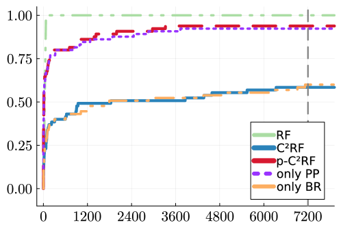
Figure 1. ECDFs for run times (in seconds)

Table 2. Median of run times (in seconds)

ID	RF	C2RF	p-C2RF	only PP	only BR
1	0.042	3859.72	2.939	3.000	1249.15
2	0.261	—	109.603	127.63	—
3	0.513	—	2.865	2.865	—
4	0.107	68.255	12.304	12.495	76.813
5	0.074	—	999.798	1018.56	—
6	0.069	—	—	—	—
7	0.172	1834.94	4.054	4.149	—
8	0.058	3.791	0.168	0.191	3.585
9	0.087	899.891	1.599	1.568	1018.80
10	0.066	883.18	144.127	182.252	—
11	1.129	—	204.337	147.684	—
12	0.194	70.102	14.443	12.619	75.937
13	0.229	0.986	0.275	0.367	1.124

In Table 2 we present the median run times of the 5 biased samples for each instance. A “—” means that the approach did not solve at least $3$ of the samples of the instance within the time limit. Once can see that RF almost always takes less than $1\text{\,}\mathrm{s}$ to solve the problem. When comparing the two novel approaches and only the instances that C²RF solves at least one sample, Table 2 shows that our techniques decrease the time computation by $89\text{\,}\mathrm{\char 37\relax}$ on average.

5.5. Discussion of Accuracy and MCC

Observe that for both metrics $\overline{\text{AC}}$ and $\overline{\text{MCC}}$, a value greater than zero indicates that p-C²RF had a better result than RF. Besides that, the box in the boxplot depicts the range of the medium $50\text{\,}\mathrm{\char 37\relax}$ of the values; $25\text{\,}\mathrm{\char 37\relax}$ of the values are below and $25\text{\,}\mathrm{\char 37\relax}$ are above the box. Figure 2 shows that the $\overline{\text{AC}}$ values are greater than zero in $75\text{\,}\mathrm{\char 37\relax}$ of the results (left plot). Hence, our proposed method has better accuracy than the conventional random forest. It can also be seen in Figure 2 that the $\overline{\text{MCC}}$ values are greater than zero in most cases (right plot). Therefore, our method has a better MCC than RF.

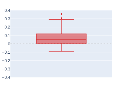
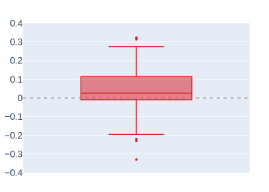
Figure 2. Comparison of $\overline{\text{AC}}$ (left) and $\overline{\text{MCC}}$ (right); see (10)

Table 3. Median of AC and MCC (in percentage)

ID	Accuracy		MCC
	RF	p-C2RF	RF	p-C2RF
1	62.16	72.51	69.28	69.20
2	65.14	75.03	70.35	73.13
3	76.28	77.78	55.66	67.16
4	61.98	79.64	55.17	57.09
5	50.80	60.20	54.20	61.45
6	58.90	66.93	65.76	67.05
7	75.88	78.59	78.55	76.47
8	98.58	98.74	84.03	84.73
9	81.30	87.59	83.95	87.57
10	61.35	71.13	71.14	70.00
11	24.79	56.69	52.19	55.98
12	89.10	88.72	54.61	53.57
13	99.43	100	98.89	100

When comparing each instance, Table 3 shows the median of AC and MCC of the 5 biased samples for RF and p-C²RF. It can be seen that, in the majority of instances, our approach has a greater value of accuracy and MCC than RF. Especially in terms of accuracy, we obtained a better median value in 12 of the 13 instances. Regarding MCC, our approach has a better median value than RF in 8 of the 13 instances. When RF has better MCC than p-C²RF, it is never better than $2.5\text{\,}\mathrm{\char 37\relax}$.

Figure 2 and Table 3 show that using the cardinality constraint of each class as additional information allows to correctly classify the points with higher accuracy and better MCC than with the RF by majority vote.

6. Conclusion

For several classification problems, it can be expensive to acquire labels for the entire population of interest. Nevertheless, external sources can, in some cases, offer additional information on how many points are in each class. For the case of binary classification, we proposed a semi-supervised random forest that can be modeled using a big-$M$-based MILP formulation. We also presented problem-tailored preprocessing techniques and a branching rule to reduce the computational cost of solving the MILP model.

Under the condition of simple random sampling, our proposed semi-supervised method has very similar accuracy and MCC as a standard random forest. In many applications, however, the available data come from non-probability samples. In this case, the data collection mechanism is largely unknown and there is the risk of obtaining biased samples. Our numerical results show that our model has better accuracy and MCC than the conventional random forest even with a small number of labeled points and biased samples.

Appendix A Numerical Results for Simple random samples

In Section 5 we present a computational study on non-representative biased samples. To complement our numerical results, we also present the results for simple random sampling. For simple random sampling, each element in the data set has the same probability $(n/N)$ to be included in the sample of labeled data of size $n$. The instances are the same as described in Section 5.1. The computational setup follows the description in Section 5.2. As before, the used evaluation criteria are $\overline{\text{AC}}$ and $\overline{\text{MCC}}$ as in (10).

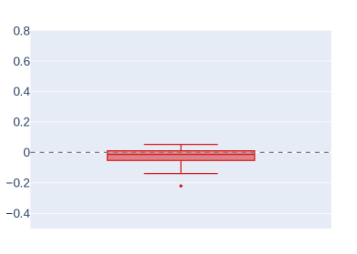
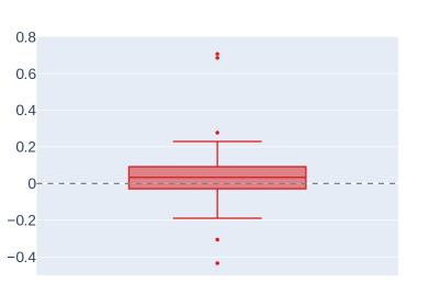
Figure 3. Comparison of $\overline{\text{AC}}$ (left) and $\overline{\text{MCC}}$ (right); see (10)

It can be seen in Figure 3 that $75\text{\,}\mathrm{\char 37\relax}$ of the values of $\overline{\text{AC}}$ are between $-0.05$ and $0.05$ (left plot). Figure 3 (right plot) also shows that $\overline{\text{MCC}}$ has a value greater than 0 and lower than 0 in $50\text{\,}\mathrm{\char 37\relax}$ of the cases.

Table 4 shows the median of AC and MCC for each instance for p-C²RF and RF. In the majority of instances, our approach has a better or a very similar accuracy and MCC compared to the conventional random forest. Especially in terms of MCC, this is the case for all 13 instances. From Figure 3 and Table 4 we can conclude that the accuracy and MCC of our proposed method p-C²RF and the standard random forest are very similar in the context of simple random sampling. This is expected because the cardinality constraint aims to balance the class distribution and since the sample is not biased, this constraint does not introduce additional meaningful information to the problem.

Table 4. Median of AC and MCC (in percentage)

ID	Accuracy		MCC
	RF	p-C2RF	RF	p-C2RF
1	76.68	76.32	71.73	71.34
2	78.28	78.14	75.82	75.86
3	81.32	80.85	70.79	73.70
4	85.86	76.57	50.0	51.63
5	71.81	67.35	72.61	67.35
6	84.32	85.09	85.32	85.10
7	76.75	77.10	71.97	74.10
8	97.68	98.61	50.0	84.43
9	88.15	87.17	88.17	87.15
10	78.57	79.84	75.13	77.23
11	75.36	67.71	50.0	55.89
12	93.23	87.01	50.0	52.62
13	97.64	100	95.37	100

References

- [1] Massih-Reza Amini and Patrick Gallinari “Semi-Supervised Logistic Regression” In Proceedings of the 15th European Conference on Artificial Intelligence, ECAI’02 Lyon, France: IOS Press, 2002, pp. 390–394
- [2] Gérard Biau and Erwan Scornet “A random forest guided tour” In TEST: An Official Journal of the Spanish Society of Statistics and Operations Research 25.2, 2016, pp. 197–227 DOI: 0.1007/s11749-016-0481-7
- [3] Leo Breiman “Random Forests” In Machine Learning 45.1 Kluwer Academic Publishers, 2001, pp. 5–32 DOI: 10.1023/A:1010933404324
- [4] Jan Pablo Burgard, Joscha Krause and Simon Schmaus “Estimation of regional transition probabilities for spatial dynamic microsimulations from survey data lacking in regional detail” In Computational Statistics & Data Analysis 154, 2021, pp. 107048 DOI: 10.1016/j.csda.2020.107048
- [5] Jan Pablo Burgard, Maria Eduarda Pinheiro and Martin Schmidt “Mixed-Integer Linear Optimization for Semi-Supervised Optimal Classification Trees”, 2024 arXiv:2401.09848 [math.OC]
- [6] Jan Pablo Burgard, Maria Eduarda Pinheiro and Martin Schmidt “Mixed-integer quadratic optimization and iterative clustering techniques for semi-supervised support vector machines” To appear In TOP, 2024 DOI: 10.1007/s11750-024-00668-w
- [7] Danilo Bzdok et al. “Semi-Supervised Factored Logistic Regression for High-Dimensional Neuroimaging Data” In Advances in Neural Information Processing Systems 28 Cambridge, MA, USA: MIT Press, 2015, pp. 3348–3356
- [8] Olivier Chapelle, Mingmin Chi and Alexander Zien “A Continuation Method for Semi-Supervised SVMs” In Proceedings of the 23rd International Conference on Machine Learning, ICML ’06 New York, NY, USA: Association for Computing Machinery, 2006, pp. 185–192 DOI: 10.1145/1143844.1143868
- [9] Adele Cutler, D. Richard Cutler and John R. Stevens “Random Forests” In Ensemble Machine Learning: Methods and Applications New York, NY: Springer New York, 2012, pp. 157–175 DOI: 10.1007/978-1-4419-9326-7_5
- [10] Nejdet Dogru and Abdulhamit Subasi “Traffic accident detection using random forest classifier” In 2018 15th learning and technology conference (L&T), 2018, pp. 40–45 IEEE DOI: 10.1109/LT.2018.8368509
- [11] Iain Dunning, Joey Huchette and Miles Lubin “JuMP: A Modeling Language for Mathematical Optimization” In SIAM Review 59.2, 2017, pp. 295–320 DOI: 10.1137/15M1020575
- [12] Vishan Kumar Gupta, Avdhesh Gupta, Dinesh Kumar and Anjali Sardana “Prediction of COVID-19 confirmed, death, and cured cases in India using random forest model” In Big Data Mining and Analytics 4.2, 2021, pp. 116–123 DOI: 10.26599/BDMA.2020.9020016
- [13] Trevor Hastie, Robert Tibshirani and Jerome Friedman “The elements of statistical learning: data mining, inference and prediction” Springer, 2009 DOI: 10.1007/978-0-387-84858-7
- [14] Kyoungok Kim “A hybrid classification algorithm by subspace partitioning through semi-supervised decision tree” In Pattern Recognition 60, 2016, pp. 157–163 DOI: 10.1016/j.patcog.2016.04.016
- [15] Michelangelo Cćeci Dragi Kocev, Jurica Levatić and Sašo Džeroski “Semi-supervised classification trees” In Journal of Intelligent Information Systems 49, 2017, pp. 461–486 DOI: 10.1007/s10844-017-0457-4
- [16] Dong-Hyun Lee “Pseudo-Label : The Simple and Efficient Semi-Supervised Learning Method for Deep Neural Networks” In ICML 2013 Workshop : Challenges in Representation Learning (WREPL), 2013
- [17] Christian Leistner, Amir Saffari, Jakob Santner and Horst Bischof “Semi-Supervised Random Forests” In 2009 IEEE 12th International Conference on Computer Vision, 2009, pp. 506–513 DOI: 10.1109/ICCV.2009.5459198
- [18] Ming Li and Zhi-Hua Zhou “Improve Computer-Aided Diagnosis With Machine Learning Techniques Using Undiagnosed Samples” In IEEE Transactions on Systems, Man, and Cybernetics - Part A: Systems and Humans 37.6, 2007, pp. 1088–1098 DOI: 10.1109/TSMCA.2007.904745
- [19] Stefano Melacci and Mikhail Belkin “Laplacian Support Vector Machines Trained in the Primal” In Journal of Machine Learning Research 12, 2009 DOI: 10.48550/ARXIV.0909.5422
- [20] Thao N. N. Nguyen, Bharadwaj Veeravalli and Xuanyao Fong “A Semi-Supervised Learning Method for Spiking Neural Networks Based on Pseudo-Labeling” In 2023 International Joint Conference on Neural Networks (IJCNN), 2023, pp. 1–7 DOI: 10.1109/IJCNN54540.2023.10191317
- [21] Avital Oliver et al. “Realistic Evaluation of Deep Semi-Supervised Learning Algorithms” In Advances in Neural Information Processing Systems 31 Curran Associates, Inc., 2018 DOI: 10.48550/arXiv.1804.09170
- [22] Randal S. Olson et al. “PMLB: a large benchmark suite for machine learning evaluation and comparison” In BioData Mining 10.36, 2017, pp. 1–13 DOI: 10.1186/s13040-017-0154-4
- [23] Madhumita Pal and Smita Parija “Prediction of Heart Diseases using Random Forest” In Journal of Physics: Conference Series 1817.1 IOP Publishing, 2021, pp. 012009 DOI: 10.1088/1742-6596/1817/1/012009
- [24] Ben Sadeghi et al. “DecisionTree.jl - A Julia implementation of the CART Decision Tree and Random Forest algorithms” Zenodo, 2022 DOI: 10.5281/zenodo.7359268
- [25] Jamie Shotton et al. “Real-time human pose recognition in parts from single depth images” In CVPR 2011, 2011, pp. 1297–1304 DOI: 10.1109/CVPR.2011.5995316
- [26] C. J. Skinner and D’arrigo “Inverse probability weighting for clustered nonresponse” In Biometrika 98.4, 2011, pp. 953–966 DOI: 10.1093/biomet/asr058
- [27] Shiyang Xuan et al. “Random forest for credit card fraud detection” In 2018 IEEE 15th International Conference on Networking, Sensing and Control (ICNSC), 2018, pp. 1–6 DOI: 10.1109/ICNSC.2018.8361343
- [28] Youqiang Zhang et al. “Active Semi-Supervised Random Forest for Hyperspectral Image Classification” In Remote Sensing 11.24, 2019 DOI: 10.3390/rs11242974
- [29] Arman Zharmagambetov and Miguel A. Carreira-Perpinan “Semi-Supervised Learning with Decision Trees: Graph Laplacian Tree Alternating Optimization” In Advances in Neural Information Processing Systems 35, 2022, pp. 2392–2405
- [30] Xiaojin Zhu and Andrew B. Goldberg “Introduction to Semi-Supervised Learning” In Introduction to Semi-Supervised Learning, Synthesis Lectures on Artificial Intelligence and Machine Learning Morgan & Claypool Publishers, 2009 DOI: 10.2200/S00196ED1V01Y200906AIM006