Nearly Minimax Optimal Regret for Multinomial Logistic Bandit

Abstract

In this paper, we study the contextual multinomial logit (MNL) bandit problem in which a learning agent sequentially selects an assortment based on contextual information, and user feedback follows an MNL choice model. There has been a significant discrepancy between lower and upper regret bounds, particularly regarding the feature dimension $d$ and the maximum assortment size $K$. Additionally, the variation in reward structures between these bounds complicates the quest for optimality. Under uniform rewards, where all items have the same expected reward, we establish a regret lower bound of $\Omega(d\sqrt{\smash[b]{T/K}})$ and propose a constant-time algorithm, OFU-MNL+, that achieves a matching upper bound of $\tilde{\mathcal{O}}(d\sqrt{\smash[b]{T/K}})$. Under non-uniform rewards, we prove a lower bound of $\Omega(d\sqrt{T})$ and an upper bound of $\tilde{\mathcal{O}}(d\sqrt{T})$, also achievable by OFU-MNL+. Our empirical studies support these theoretical findings. To the best of our knowledge, this is the first work in the contextual MNL bandit literature to prove minimax optimality — for either uniform or non-uniform reward setting — and to propose a computationally efficient algorithm that achieves this optimality up to logarithmic factors.

1 Introduction

The multinomial logistic (MNL) bandit framework [42, 43, 6, 7, 35, 36, 39, 4, 47] describes sequential assortment selection problems in which an agent offer a sequence of assortments of at most $K$ item from a set of $N$ possible items and receives feedback only for the chosen decisions. The choice probability of each outcome is characterized by an MNL model [32]. This framework allows modeling of various real-world situations such as recommender systems and online retails, where selections of assortments are evaluated based on the user-choice feedback among offered multiple options.

In this paper, we study the contextual MNL bandit problem [7, 6, 38, 13, 35, 36, 39, 4], where the features of items and possibly contextual information about a user at each round are available. Despite many recent advances, [13, 35, 36, 39, 4], however, no previous studies have proven the minimax optimality of contextual MNL bandits. Chen et al. [13] proposed a regret lower bound of $\Omega(d\sqrt{T}/K)$, where $d$ is the number of features, $T$ is the total number of rounds, and $K$ is the maximum size of assortments, assuming the uniform rewards, i.e., rewards are all same for each of the total $N$ items. Furthermore, Chen and Wang [12] established a regret lower bound of $\Omega(\sqrt{NT})$ in the non-contextual setting (hence, dependence on $N$ appears instead of $d$), which is tighter in terms of $K$. It is important to note the difference in the assumptions for the utility of the outside option $v_{0}$. Chen and Wang [12] assumed for the utility for the outside option to be $v_{0}=K$, whereas Chen et al. [13] assumed $v_{0}=1$. Therefore, it remains an open question whether and how the value of $v_{0}$ affects both lower and upper bounds of regret.

Regarding regret upper bounds, Chen et al. [13] proposed an exponential runtime algorithm that achieves a regret of $\tilde{\mathcal{O}}(d\sqrt{T})$ in the setting with stochastic contexts and the non-uniform rewards. Under the same setting, Oh and Iyengar [36] and Oh and Iyengar [35] introduced polynomial-time algorithms that attain regrets of $\tilde{\mathcal{O}}(d\sqrt{T}/\kappa)$ and $\tilde{\mathcal{O}}(d^{3/2}\sqrt{T}/\kappa)$ respectively, where $1/\kappa=\mathcal{O}(K^{2})$ is a problem-dependent constant. Recently, Perivier and Goyal [39] improved the dependency on $\kappa$ in the adversarial context setting, achieving a regret of $\tilde{\mathcal{O}}(dK\sqrt{\kappa^{\prime}T})$, where $\kappa^{\prime}=\mathcal{O}(1/K)$. However, their approach focuses solely on the setting with uniform rewards, which is a special case of non-uniform rewards, and currently, there is no tractable method to implement the algorithm.

As summarized in Table 1, there has been a gap between the upper and lower bounds in the existing works of contextual MNL bandits. No previous studies have confirmed whether lower or upper bounds are tight, obscuring what the optimal regret should be. This ambiguity is further exacerbated because many studies introduce their methods under varying conditions such as different reward structures and values of $v_{0}$, without explicitly explaining how these factors impact regret. Additionally, there is currently no computationally efficient algorithm whose regret does not scale with $1/\kappa=\mathcal{O}(K^{2})$ or directly with $K$. Intuitively, increasing $K$ provides more information at least in the uniform reward setting, potentially leading to a more statistically efficient learning process. However, no previous results have reflected such intuition. Hence, the following research questions arise:

• What is the optimal regret lower bound in contextual MNL bandits?

• Can we design a computationally efficient, nearly minimax optimal algorithm under the adversarial context setting?

Table 1: Comparisons of lower and upper regret bounds in related works on MNL bandits with $T$ rounds, $N$ items, the maximum size of assortments $K$, $d$-dimensional feature vectors, and problem-dependent constants $1/\kappa=\mathcal{O}(K^{2})$ and $\kappa^{\prime}=\mathcal{O}(1/K)$. $\tilde{\mathcal{O}}$ represents big-$\mathcal{O}$ notation up to logarithmic factors. For the computational cost (abbreviated as “Comput.”), we consider only the dependence on the number of rounds $t$. “Intractable” means a non-polynomial runtime. The notation “$-$” denotes not applicable. The starred (^∗) papers only consider the non-contextual setting.

		Regret	Contexts	Rewards	$v_{0}$	Comput. per Round
Lower Bound	Chen et al. [13]	$\Omega(d\sqrt{T}/K)$	$-$	Uniform	$\Theta(1)$	$-$
	Agrawal et al. [7]∗	$\Omega(\sqrt{NT/K})$	$-$	Uniform	$\Theta(K)$	$-$
	Chen and Wang [12]∗	$\Omega(\sqrt{NT})$	$-$	Uniform	$\Theta(K)$	$-$
	This work (Theorem 1)	$\Omega(\frac{\sqrt{v_{0}K}}{v_{0}+K}d\sqrt{T})$	$-$	Uniform	Any value	$-$
	This work (Theorem 3)	$\Omega(d\sqrt{T})$	$-$	Non-uniform	$\Theta(1)$	$-$
Upper Bound	Chen et al. [13]	$\tilde{\mathcal{O}}(d\sqrt{T})$	Stochastic	Non-uniform	$\Theta(1)$	Intractable
	Oh and Iyengar [36]	$\tilde{\mathcal{O}}(d\sqrt{T}/\kappa)$	Stochastic	Non-uniform	$\Theta(1)$	$\mathcal{O}(t)$
	Oh and Iyengar [35]	$\tilde{\mathcal{O}}(d^{3/2}\sqrt{T}/\kappa)$	Adversarial	Non-uniform	$\Theta(1)$	$\mathcal{O}(t)$
	Perivier and Goyal [39]	$\tilde{\mathcal{O}}(dK\sqrt{\kappa^{\prime}T})$	Adversarial	Uniform	$\Theta(1)$	Intractable
	This work (Theorem 2)	$\tilde{\mathcal{O}}\left(\frac{\sqrt{v_{0}K}}{v_{0}+K}d\sqrt{T}\right)$	Adversarial	Uniform	Any value	$\mathcal{O}(1)$
	This work (Theorem 4)	$\tilde{\mathcal{O}}(d\sqrt{T})$	Adversarial	Non-uniform	$\Theta(1)$	$\mathcal{O}(1)$

In this paper, we affirmatively answer the questions by first tackling the contextual MNL bandit problem separately based on the structure of rewards—uniform and non-uniform—and the value of the outside option $v_{0}$. In the setting of uniform rewards, we establish the tightest regret lower bound, explicitly demonstrating the dependence of regret on $v_{0}$. Specifically, we prove a regret lower bound of $\Omega(d\sqrt{\smash[b]{T/K}})$ when $v_{0}=\Theta(1)$, a common assumption in contextual settings [42, 5, 15, 38, 7, 35, 36, 8, 39, 4, 47, 29] (see Appendix C.1 for more details), and a lower bound of $\Omega(d\sqrt{T})$ when $v_{0}=\Theta(K)$. Furthermore, in the adversarial context setting, we introduce a computationally efficient and provably optimal (up to logarithmic factors) algorithm, OFU-MNL+. We prove that our proposed algorithm achieves a regret of $\tilde{\mathcal{O}}(d\sqrt{T/K})$ when $v_{0}=\Theta(1)$ and $\tilde{\mathcal{O}}(d\sqrt{T})$ when $v_{0}=\Theta(K)$, each of which matches the respective lower bounds that we establish up to logarithmic factors. Furthermore, in the non-uniform reward setting, we provide the optimal lower bound of $\Omega(d\sqrt{T})$ assuming $v_{0}=\Theta(1)$. In the same setting, our proposed algorithm also attains a matching upper bound of $\tilde{\mathcal{O}}(d\sqrt{T})$ up to logarithmic factors. Our main contributions are summarized as follows:

• Under uniform rewards, we establish a regret lower bound of $\Omega(\sqrt{v_{0}K}/(v_{0}+K)d\sqrt{T})$, which is the tightest known lower bound in contextual MNL bandits. We propose, for the first time, a computationally efficient and provably optimal algorithm, OFU-MNL+, achieving a matching upper bound of $\mathcal{O}(\sqrt{v_{0}K}/(v_{0}+K)d\sqrt{T})$ up to logarithmic factors, while requiring only a constant computation cost per round. The results indicate that the regret improves as the assortment size $K$ increases, unless $v_{0}=\Theta(K)$. To the best of our knowledge, this is the first study to demonstrate the dependence of regret on the utility for the outside option $v_{0}$ and to highlight the advantages of a larger assortment size $K$ which aligns with intuition. That is, this is the first work to show that a regret upper bound (in either contextual or non-contextual setting) decreases as $K$ increases.

• Under non-uniform rewards, with setting $v_{0}=\Theta(1)$ following the convention in contextual MNL bandits [42, 5, 15, 38, 7, 35, 36, 8, 39, 4, 47, 29], we establish a regret lower bound of $\Omega(d\sqrt{T})$. To the best of our knowledge, this is the first and tightest lower bound established under non-uniform rewards. Moreover, OFU-MNL+ also achieves a matching upper bound (up to logarithmic factors) of $\tilde{\mathcal{O}}(d\sqrt{T})$ in this setting.

• We also conduct numerical experiments and show that our algorithm consistently outperforms the existing MNL bandit algorithms while maintaining a constant computation cost per round. Furthermore, the empirical results corroborate our theoretical findings regarding the dependence of regret on the reward structure, $v_{0}$ and $K$.

Overall, our paper addresses the long-standing open problem of closing the gap between upper and lower bounds for contextual MNL bandits. Our proposed algorithm is the first to achieve both provably optimality (up to logarithmic factors) and practicality with improved computation.

2 Related Work

Lower bounds of MNL bandits. In contextual MNL bandits, to the best of our knowledge, only Chen et al. [13] proved a lower bound of $\Omega(d\sqrt{T}/K)$ with the utility for the outside option set at $v_{0}=1$. However, in the non-contextual setting, there exist improved lower bounds in terms of $K$.  Agrawal et al. [7] demonstrated a lower bound of $\Omega(\sqrt{NT/K})$, and Chen and Wang [12] established a lower bound of $\Omega(\sqrt{NT})$. By setting $d=N$, one can derive equivalent lower bounds for the contextual setting, specifically $\Omega(\sqrt{dT/K})$ and $\Omega(\sqrt{dT})$, respectively. However, Agrawal et al. [7] and Chen and Wang [12] assumed $v_{0}=K$ when establishing their lower bounds, which differs from the setting used by Chen et al. [13], where $v_{0}=1$. Moreover, to the best of our knowledge, all existing works Chen et al. [13], Agrawal et al. [7], Chen and Wang [12] have established the lower bounds under uniform rewards. Consequently, it remains unclear what the optimal regret is, depending on the value of $v_{0}$ and the reward structure.

Upper bounds of contextual MNL bandits. Ou et al. [38] formulated a linear utility model and achieved $\tilde{\mathcal{O}}(dK\sqrt{T})$ regret; however, they assumed that utilities are fixed over time. Chen et al. [13] considered contextual MNL bandits with changing and stochastic contexts, establishing a regret of $\tilde{\mathcal{O}}(d\sqrt{T}+d^{2}K^{2})$. However, they encountered computational issues due to the need to enumerate all possible ($N$ choose $K$) assortments. To address this, Oh and Iyengar [36] proposed a polynomial-time assortment optimization algorithm, which maintains the confidence bounds in the parameter space and then calculates the upper confidence bounds of utility for each items, achieving a regret of $\tilde{\mathcal{O}}(d\sqrt{T}/\kappa)$, where $1/\kappa=\mathcal{O}(K^{2})$ is a problem-dependent constant. Perivier and Goyal [39] considered the adversarial context and uniform reward setting and improved the dependency on $\kappa$ to $\tilde{\mathcal{O}}(dK\sqrt{\kappa^{\prime}T}+d^{2}K^{4}/\kappa)$, where $\kappa^{\prime}=\mathcal{O}(1/K)$. However, their algorithm is intractable. Recently, Zhang and Sugiyama [47] utilized an online parameter update to construct a constant time algorithm. However, they consider a multiple-parameter choice model in which the learner estimates $K$ parameters and shares the contextual information $x_{t}$ across the items in the assortment. This model differs from ours; we use a single-parameter choice model with varying the context for each item in the assortment. Additionally, they make a stronger assumption regarding the reward than we do (see Assumption 1). Moreover, while they fix the assortment size at $K$, we allow it to be smaller than or equal to $K$. To the best of our knowledge, all existing methods fail to show that the regret upper bound can improve as the assortment size $K$ increases.

3 Existing Gap between Upper and Lower Bounds in MNL Bandits

The primary objective of this paper is to bridge the existing gap between the upper and lower bounds and to establish minimax regrets in contextual MNL bandits. To explore the optimality of regret, we analyze how it depends on the utility of the outside option $v_{0}$, the maximum assortment size $K$, and the structure of rewards.

Dependence on $v_{0}$. Currently, the established lower bounds are $\Omega(d\sqrt{T}/K)$ by Chen et al. [13], $\Omega(\sqrt{\smash[b]{dT/K}})$ by the contextual version of Agrawal et al. [7], and $\Omega(\sqrt{dT})$, which is the tightest in terms of $K$, by the contextual version of Chen and Wang [12]. These results can be misleading, as many subsequent studies [36, 34, 14, 46] have claimed that a $K$-independent regret is achievable, without clearly addressing the influence of the value of $v_{0}$. In fact, the improved regret bounds (in terms of $K$) obtained by Agrawal et al. [7] and Chen and Wang [12] were possible when $v_{0}=K$. However, in the contextual setting, it is more common to set $v_{0}=\Theta(1)$. This is because, given the context for the outside option $x_{t0}$, it is straightforward to construct an equivalent choice model where $v_{0}=\Theta(1)$ (refer Appendix C.1). In this paper, under uniform rewards ($r_{ti}=1$), we rigorously show the regret dependency on the value of $v_{0}$. In Theorem 1, we establish a regret lower bound of $\Omega\left(\sqrt{v_{0}K}/(v_{0}+K)d\sqrt{T}\right)$, which implies that the value of $v_{0}$, indeed, affects the regret. Then, in Theorem 2, we show that our proposed computationally efficient algorithm, OFU-MNL+ achieves a regret of $\tilde{\mathcal{O}}\left(\sqrt{v_{0}K}/(v_{0}+K)d\sqrt{T}\right)$, which is minimax optimal up to logarithmic factors in terms of all $d,T,K$ and even $v_{0}$.

Dependence on $K$ & Uniform/Non-uniform rewards. To the best of our knowledge, the regret bound in all existing works in contextual MNL bandits does not decrease as the assortment size $K$ increases [13, 35, 36, 39]. However, intuitively, as the assortment size increases, we can gain more information because we receive more feedback. Therefore, it makes sense that regret could be reduced as $K$ increases, at least in the uniform reward setting. Under uniform rewards, the expected revenue (to be specified later) increases as more items are added in the assortment. Consequently, both the optimistically chosen assortment and the optimal assortment always have a size of $K$. Thus, the agent obtain information about exactly $K$ items in each round. This phenomenon is also demonstrated empirically in Figure 1. In the uniform reward setting, as $K$ increases, the cumulative regrets of not only our proposed algorithm but also other baseline algorithms decrease. This indicates that the existing regret bounds are not tight enough in terms of $K$. Conversely, in the non-uniform reward setting, the sizes of both the optimistically chosen assortment and the optimal assortment can be less than $K$, so performance improvement is not guaranteed. In this paper, we show that the regret dependence on $K$ varies by case: uniform and non-uniform rewards. When $v_{0}=\Theta(1)$, we obtain a regret lower bound of $\Omega(d\sqrt{\smash[b]{T/K}})$ (Theorem 1) and a regret upper bound of $\tilde{\mathcal{O}}(d\sqrt{\smash[b]{T/K}})$ (Theorem 2) under uniform rewards. Additionally, we achieve a regret lower bound of (Theorem 3) and a regret upper bound of $\tilde{\mathcal{O}}(d\sqrt{T})$ (Theorem 4) under non-uniform rewards.

4 Problem Setting

Notations. For a positive integer, $n$, we denote $[n]:=\{1,2,\ldots,n\}$. For a real-valued matrix $A$, we denotes $\|A\|_{2}:=\sup_{x:\|x\|_{2}=1}\|Ax\|_{2}$ as the maximum singular value of $A$. For two symmetric matrices, $V$ and $W$ of the same dimensions, $V\succeq W$ means that $V-W$ is positive semi-definite. Finally, we define $\mathcal{S}$ to be the set of candidate assortment with size constraint at most $K$, i.e., $\mathcal{S}=\{S\subset[N]:|S|\leq K\}$. While, for simplicity, we consider both $\mathcal{S}$ and the set of items $[N]$ to be stationary in this paper, it is important to note that both $\mathcal{S}$ and $[N]$ can vary over time.

Contextual MNL bandits. We consider a sequential assortment selection problem which is defined as follows. At each round $t$, the agent observes feature vectors $x_{ti}\in\mathbb{R}^{d}$ for every item $i\in[N]$. Based on this contextual information, the agent presents an assortment $S_{t}=\{i_{1},\dots,i_{l}\}\in\mathcal{S}$, where $l\leq K$, and then observes the user purchase decision $c_{t}\in S_{t}\cup\{0\}$, where $\{0\}$ represents the “outside option” which indicates that the user did not select any of the items in $S_{t}$. The distribution of these selections follows a multinomial logit (MNL) choice model [32], where the probability of choosing any item $i_{k}\in S_{t}$ (or the outside option) is defined as:

$$p_{t}(i_{k}|S_{t},\mathbf{w}^{\star}):=\frac{\exp(x_{ti_{k}}^{\top}\mathbf{w}^{\star})}{v_{0}\!+\!\sum_{j\in S_{t}}\exp(x_{tj}^{\top}\mathbf{w}^{\star})},\quad p_{t}(0|S_{t},\mathbf{w}^{\star}):=\frac{v_{0}}{v_{0}\!+\!\sum_{j\in S_{t}}\exp(x_{tj}^{\top}\mathbf{w}^{\star})},$$ (1)

where $v_{0}$ is a known utility for the outside option and $\mathbf{w}^{\star}\in\mathbb{R}^{d}$ is an unknown parameter.

Remark 1.

In the existing literature on MNL bandits, it is commonly assumed that $v_{0}=1$ [35, 36, 39, 4, 47]. On the other hand, Chen and Wang [12], Agrawal et al. [7] assume that $v_{0}=K$  to induce a tighter lower bound in terms of $K$. Later, we will explore how these differing assumptions create fundamentally different problems, leading to different regret lower bounds (Subsection 5.1).

The choice response for each item $i\in S_{t}\cup\{0\}$ is defined as $y_{ti}:=\mathbbm{1}(c_{t}=i)\in\{0,1\}$. Hence, the choice feedback variable $\mathbf{y}_{t}:=(y_{t0},y_{ti_{1}},\dots y_{ti_{l}})$ is sampled from the following multinomial (MNL) distribution: $\mathbf{y}_{t}\sim\operatorname{MNL}\{1,(p_{t}(0|S_{t},\mathbf{w}^{\star}),\dots,p_{t}(i_{l}|S_{t},\mathbf{w}^{\star}))\}$, where the parameter 1 indicates that $\mathbf{y}_{t}$ is a single-trial sample, i.e., $y_{t0}+\sum_{k=1}^{l}y_{ti_{k}}=1$. For each $i\in S_{t}\cup\{0\}$, we define the noise $\epsilon_{ti}:=y_{ti}-p_{t}(i|S_{t},\mathbf{w}^{\star})$. Since each $\epsilon_{ti}$ is a bounded random variable in $[0,1]$, $\epsilon_{ti}$ is $1/4$-sub-Gaussian. At every round $t$, the reward $r_{ti}$ for each item $i$ is also given. Then, we define the expected revenue of the assortment $S$ as

$$R_{t}(S,\mathbf{w}^{\star}):=\sum_{i\in S}p_{t}(i|S,\mathbf{w}^{\star})r_{ti}=\frac{\sum_{i\in S}\exp(x_{ti}^{\top}\mathbf{w}^{\star})r_{ti}}{v_{0}\!+\!\sum_{j\in S}\exp(x_{tj}^{\top}\mathbf{w}^{\star})}$$

and define $S_{t}^{\star}$ as the offline optimal assortment at time $t$ when $\mathbf{w}^{\star}$ is known a prior, i.e., $S_{t}^{\star}=\mathop{\mathrm{argmax}}_{S\in\mathcal{S}}\sum_{i\in S}R_{t}(S,\mathbf{w}^{\star})$. Our objective is to minimize the cumulative regret over the $T$ periods:

$$\textup{{Reg}}_{T}(\mathbf{w}^{\star})=\sum_{t=1}^{T}R_{t}(S_{t}^{\star},\mathbf{w}^{\star})-R_{t}(S_{t},\mathbf{w}^{\star}).$$

When $K=1$, $r_{t1}=1$, and $v_{0}=1$, the MNL bandit recovers the binary logistic bandit with $R_{t}(S=\{x\},\mathbf{w}^{\star})=\sigma\left(x^{\top}\mathbf{w}^{\star}\right)=1/(1+\exp(-x^{\top}\mathbf{w}^{\star}))$, where $\sigma(\cdot)$ is the sigmoid function.

Consistent with previous works on MNL bandits [36, 39, 4, 47], we make the following assumptions:

Assumption 1 (Bounded assumption).

We assume that $\|\mathbf{w}^{\star}\|_{2}\leq 1$, and for all $t\geq 1$, $i\in[N]$, $\|x_{ti}\|_{2}\leq 1$ and $r_{ti}\in[0,1]$.

Assumption 2 (Problem-dependent constant).

There exist $\kappa>0$ such that for every item $i\in S$ and any $S\in\mathcal{S}$, and all round $t$, $\min_{\mathbf{w}\in\mathcal{W}}p_{t}(i|S,\mathbf{w})p_{t}(0|S,\mathbf{w})\geq\kappa$, where $\mathcal{W}=\{\mathbf{w}\in\mathbb{R}^{d}\mid\|\mathbf{w}\|_{2}\leq 1\}$.

In Assumption 1, we assume that the reward for each item $i$ is bounded by a constant, allowing the norm of the reward vector to depend on $K$, e.g., $\|\bm{\rho}_{t}\|_{2}\leq\sqrt{K}$. In contrast, Zhang and Sugiyama [47] assume that the norm of the reward vector $\bm{\rho}_{t}=[r_{t1},\dots r_{t|S_{t}|}]^{\top}\in\mathbb{R}^{|S_{t}|}$ is bounded by a constant, independent of $K$, e.g., $\|\bm{\rho}_{t}\|_{2}\leq 1$. Thus, our assumption regarding rewards is weaker than theirs.

Assumption 2 is common in contextual MNL bandits [13, 36, 39, 47]. Note that $1/\kappa$ depends on the maximum size of the assortment $K$, i.e., $1/\kappa=\mathcal{O}(K^{2})$. One of the primary goals of this paper is to show that as the assortment size $K$ increases, we can achieve an improved (or at least not worsened) regret bound. To this end, we design a dynamic assortment policy that enjoys improved dependence on $\kappa$. Note that our algorithm does not need to know $\kappa$ a priori, whereas Oh and Iyengar [35, 36] do.

5 Algorithms and Main Results

In this section, we begin by proving the tightest regret lower bound under uniform rewards (Subsection 5.1), explicitly showing the dependence on the utility for the outside option $v_{0}$. We then introduce OFU-MNL+, an algorithm that achieves minimax optimality, up to logarithmic factors under uniform rewards (Subsection 5.2). Notably, OFU-MNL+ is designed for efficiency, requiring only an $\mathcal{O}(Kd^{3})$ computation cost per iteration and an $\mathcal{O}(d^{2})$ storage cost. Finally, we establish the tightest regret lower bound and a matching minimax optimal regret upper bound (up to logarithmic factors) under non-uniform rewards (Subsection 5.3).

5.1 Regret Lower Bound under Uniform Rewards

In this subsection, we present a lower bound for the worst-case expected regret in the uniform reward setting ($r_{ti}=1$). This covers all applications where the objective is to maximize the appropriate “click-through rate” by offering the assortment.

Theorem 1 (Regret lower bound, Uniform rewards).

Let $d$ be divisible by $4$ and let Assumption 1 hold true. Suppose $T\geq C\cdot d^{4}(v_{0}+K)/K$ for some constant $C>0$. Then, in the uniform reward setting, for any policy $\pi$, there exists a worst-case problem instance with $N=\Theta(K\cdot 2^{d})$ items such that the worst-case expected regret of $\pi$ is lower bounded as follows:

$$\sup_{\mathbf{w}}\mathbb{E}^{\pi}_{\mathbf{w}}\left[\textup{{Reg}}_{T}(\mathbf{w})\right]=\Omega\left(\frac{\sqrt{v_{0}K}}{v_{0}+K}\cdot d\sqrt{T}\right).$$

Discussion of Theorem 1. If $v_{0}=\Theta(1)$, Theorem 1 demonstrates a regret lower bound of $\Omega(d\sqrt{\smash[b]{T/K}})$. This indicates that, under uniform rewards, increasing the assortment size $K$ leads to an improvement in regret. Compared to the lower bound $\Omega(d\sqrt{T}/K)$ proposed by Chen et al. [13], our lower bound is improved by a factor of $\sqrt{K}$. This improvement is mainly due to the establishment of a tighter upper bound for the KL divergence (Lemma D.2). Notably, Chen et al. [13] also considered uniform rewards with $v_{0}=\Theta(1)$. On the other hand, Chen and Wang [12] and Agrawal et al. [7] established regret lower bounds of $\Omega(\sqrt{NT})$ and $\Omega(\sqrt{NT/K})$, respectively, in non-contextual MNL bandits with uniform rewards, by setting $v_{0}=K$ to achieve these regrets. Theorem 1 shows that if $v_{0}=\Theta(K)$, we can obtain a regret lower bound of $\Omega(d\sqrt{T})$, which is consistent with the $K$-independent regret in Chen and Wang [12]. To the best of our knowledge, this result is the first to explicitly show the dependency of regret on the utility for the outside option $v_{0}$.

5.2 Minimax Optimal Regret Upper Bound under Uniform Rewards

In this subsection, we propose a new algorithm OFU-MNL+, which enjoys minimax optimal regret up to logarithmic factors in the case of uniform rewards. Note that, since the revenue is an increasing function when rewards are uniform, maximizing the expected revenue $R_{t}(S,\mathbf{w})$ over all $S\in\mathcal{S}$ always yields exactly $K$ items, i.e., $|S_{t}|=|S_{t}^{\star}|=K$.

Our first step involves constructing the confidence set for the online parameter.

Online parameter estimation. Instead of performing MLE as in previous works works [13, 36, 39], inspired by Zhang and Sugiyama [47], we use the mirror descent algorithm to estimate parameter. We first define the multinomial logistic loss function at round $t$ as:

$$\ell_{t}(\mathbf{w}):=-\sum_{i\in S_{t}}y_{ti}\log p_{t}(i|S_{t},\mathbf{w}).$$ (2)

In Proposition C.1, we will show that the loss function has the constant parameter self-concordant-like property. We estimate the true parameter $\mathbf{w}^{\star}$ as follows:

$$\mathbf{w}_{t+1}=\mathop{\mathrm{argmin}}_{\mathbf{w}\in\mathcal{W}}\langle\nabla\ell_{t}(\mathbf{w}_{t}),\mathbf{w}\rangle+\frac{1}{2\eta}\|\mathbf{w}-\mathbf{w}_{t}\|_{\tilde{H}_{t}}^{2}\,,\quad\forall t\geq 1$$ (3)

where $\eta>0$ is the step-size parameter to be specified later, and $\tilde{H}_{t}:=H_{t}+\eta\mathcal{G}_{t}(\mathbf{w}_{t})$, where

$$\mathcal{G}_{t}(\mathbf{w}):=\sum_{i\in S_{t}}p_{t}(i|S_{t},\mathbf{w})x_{ti}x_{ti}^{\top}-\sum_{i\in S_{t}}\sum_{j\in S_{t}}p_{t}(i|S_{t},\mathbf{w})p_{t}(j|S_{t},\mathbf{w})x_{ti}x_{tj}^{\top},$$

and $H_{t}:=\lambda\mathbf{I}_{d}+\sum_{s=1}^{t-1}\mathcal{G}_{s}(\mathbf{w}_{s+1})$. Note that $\mathcal{G}_{t}(\mathbf{w})=\nabla^{2}\ell_{t}(\mathbf{w})$. This online estimator is efficient in terms of both computation and storage. By a standard online mirror descent formulation [37], (3) can be solved using a single projected gradient step through the following equivalent formula:

$$\mathbf{w}^{\prime}_{t+1}=\mathbf{w}_{t}-\eta\tilde{H}_{t}^{-1}\nabla\ell_{t}(\mathbf{w}_{t}),\quad\text{and}\quad\mathbf{w}_{t+1}=\mathop{\mathrm{argmin}}_{\mathbf{w}\in\mathcal{W}}\|\mathbf{w}-\mathbf{w}^{\prime}_{t+1}\|_{\tilde{H}_{t}},$$ (4)

which enjoys a computational cost of only $\mathcal{O}(Kd^{3})$, completely independent of $t$ [33, 47]. Regarding storage costs, the estimator does not need to store all historical data because both $\tilde{H}_{t}$ and $H_{t}$ can be updated incrementally, requiring only $\mathcal{O}(d^{2})$ storage.

Furthermore, the estimator allows for a $\kappa$-independent confidence set, leading to an improved regret.

Lemma 1 (Online parameter confidence set).

Let $\delta\in(0,1]$. Under Assumption 1, with $\eta=\frac{1}{2}\log(K+1)+2$ and $\lambda=84\sqrt{2}d\eta$, we define the following confidence set

$$\mathcal{C}_{t}(\delta):=\{\mathbf{w}\in\mathcal{W}\mid\|\mathbf{w}_{t}-\mathbf{w}\|_{H_{t}}\leq\beta_{t}(\delta)\},$$

where $\beta_{t}(\delta)=\mathcal{O}\left(\sqrt{d}\log t\log K\right)$. Then, we have $\textup{Pr}[\forall t\geq 1,\mathbf{w}^{\star}\in\mathcal{C}_{t}(\delta)]\geq 1-\delta$.

Armed with the online estimator, we construct the computationally efficient optimistic revenue.

Algorithm 1 OFU-MNL+

1:Inputs: regularization parameter $\lambda$, probability $\delta$, confidence radius $\beta_{t}(\delta)$ ,step size $\eta$.

2:Initialize: $H_{1}=\lambda\mathbf{I}_{d}$ and $\mathbf{w}_{1}$ as any point in $\mathcal{W}$,

3:for episode $t=1,2,\cdots,T$ do

4:     Compute $\alpha_{ti}=x_{ti}^{\top}\mathbf{w}_{t}+\beta_{t}(\delta)\|x_{ti}\|_{H_{t}^{-1}}$ for all $i\in[N]$.

5:     Offer $S_{t}=\mathop{\mathrm{argmax}}_{S\in\mathcal{S}}\tilde{R}_{t}(S)$ and observe $\mathbf{y}_{t}$.

6:     Update $\tilde{H}_{t}=H_{t}+\eta\mathcal{G}_{t}(\mathbf{w}_{t})$, and update the estimator $\mathbf{w}_{t+1}$ by (3).

7:     Update $H_{t+1}=H_{t}+\mathcal{G}_{t}(\mathbf{w}_{t+1})$.

8:end for

Computationally efficient optimistic expected revenue. To balance the exploration and exploitation trade-off, we use the upper confidence bounds (UCB) technique, which have been widely studied in many bandit problems, including $K$-arm bandits [9, 36] and linear bandits [1, 16].

At each time $t$, given the confidence set in Lemma 1, we first calculate the optimistic utility $\alpha_{ti}$ for each item as follows:

$$\alpha_{ti}:=x_{ti}^{\top}\mathbf{w}_{t}+\beta_{t}(\delta)\|x_{ti}\|_{H_{t}^{-1}}.$$ (5)

The optimistic utility $\alpha_{ti}$ is composed of two parts: the mean utility estimate $x_{ti}^{\top}\mathbf{w}_{t}$ and the standard deviation $\beta_{t}(\delta)\|x_{ti}\|_{H_{t}^{-1}}$. In the proof of the regret upper bound, we show that $\alpha_{ti}$ serves as an upper bound for $x_{ti}^{\top}\mathbf{w}^{\star}$, assuming that the true parameter $\mathbf{w}^{\star}$ falls within the confidence set $\mathcal{C}_{t}(\delta)$. Based on $\alpha_{ti}$, we construct the optimistic expected revenue for the assortment $S$, defined as follows:

$$\tilde{R}_{t}(S):=\frac{\sum_{i\in S}\exp(\alpha_{ti})r_{ti}}{v_{0}+\sum_{j\in S}\exp(\alpha_{ti})},$$ (6)

where $r_{ti}=1$. Then, we offer the set $S_{t}$ that maximizes the optimistic expected revenue, $S_{t}=\mathop{\mathrm{argmax}}_{S\in\mathcal{S}}\tilde{R}_{t}(S)$. Given our assumption that all rewards are of unit value, the optimization problem is equivalent to selecting the $K$ items with the highest optimistic utility $\alpha_{ti}$. Consequently, solving the optimization problem incurs a constant computational cost of $\mathcal{O}(N)$.

Remark 2 (Comparison to Zhang and Sugiyama [47]).

In Zhang and Sugiyama [47], the MNL choice model is outlined with a shared context $x_{t}$ and distinct parameters $\mathbf{w}_{1}^{\star},\dots,\mathbf{w}_{K}^{\star}$ for each choice. Conversely, our model employs a single parameter $\mathbf{w}^{\star}$ across all choices and has varying contexts for each item in the assortment $S$, $x_{t1},\dots x_{ti_{|S|}}$. Due to this discrepancy in the choice model, directly applying Proposition 1 from Zhang and Sugiyama [47], which constructs the optimistic revenue by adding bonus terms to the estimated revenue, incurs an exponential computational cost in our problem setting. This complexity arises because the optimistic revenue must be calculated for every possible assortment $S\in\mathcal{S}$; therefore, it is necessary to enumerate all potential assortments ($N$ choose $K$) to identify the one that maximizes the optimistic revenue As a result, extending the approach in Zhang and Sugiyama [47] to our setting is non-trivial, requiring a different analysis.

We now present the regret upper bound of OFU-MNL+ in the uniform reward setting.

Theorem 2 (Regret upper bound of OFU-MNL+, Uniform rewards).

Let $\delta\in(0,1]$ and Assumptions 1 and 2 hold. In the uniform reward setting, by setting $\eta=\frac{1}{2}\log(K+1)+2$ and $\lambda=84\sqrt{2}d\eta$, with probability at least $1-\delta$, the cumulative regret of OFU-MNL+ is upper-bounded by

$$\textup{{Reg}}_{T}(\mathbf{w}^{\star})=\tilde{\mathcal{O}}\left(\frac{\sqrt{v_{0}K}}{v_{0}+K}\cdot d\sqrt{T}+\frac{1}{\kappa}d^{2}\right).$$

Discussion of Theorem 2. If $T\geq\mathcal{O}(d^{2}(v_{0}+K)^{2}/(\kappa^{2}v_{0}K))$, Theorem 2 shows that our algorithm OFU-MNL+ achieves minimax optimal regret (up to logarithmic factor) in terms of all $d$, $T$, $K$, and even $v_{0}$. To the best of our knowledge, ignoring logarithmic factors, our proposed algorithm is the first computationally efficient, minimax optimal algorithm in (adversarial) contextual MNL bandits. When $v_{0}=\Theta(1)$, which is the convention in existing MNL bandit literature [35, 36, 39, 4, 47], OFU-MNL+ obtains $\tilde{\mathcal{O}}(d\sqrt{T/K})$ regret. This represents an improvement over the previous upper bound of Perivier and Goyal [39] , which is $\tilde{\mathcal{O}}(dK\sqrt{\kappa^{\prime}T}+d^{2}K^{4}/\kappa)$, where $\kappa^{\prime}=\mathcal{O}(1/K)$, by a factor of $K$. This improvement can be attributed to two key factors: an improved, constant, self-concordant-like property of the loss function (Proposition C.1) and a $K$-free elliptical potential (Lemma E.2). Furthermore, by employing an improved bound for the second derivative of the revenue (Lemma E.3), we achieve an enhancement in the regret for the second term, $d^{2}/\kappa$, by a factor of $K^{4}$, in comparison to Perivier and Goyal [39]. Unless $v_{0}=\Theta(K)$, Theorem 2 indicates that the regret decreases as the assortment size $K$ increases. To the best of our knowledge, this is the first algorithm in MNL bandits to show that increasing $K$ results in a reduction in regret. Moreover, when reduced to the logistic bandit, i.e., $K=1$, $r_{t1}=1$, and $v_{0}=1$, our algorithm can also achieve a regret of $\tilde{\mathcal{O}}(d\sqrt{\kappa T})$ by Corollary 1 in Zhang and Sugiyama [47], which is consistent with the results in Abeille et al. [3], Faury et al. [19].

Remark 3 (Efficiency of OFU-MNL+).

The proposed algorithm is computationally efficient in both parameter updates and assortment selections. Since we employ online parameter estimation, akin to Zhang and Sugiyama [47], our algorithm demonstrates computational efficiency in parameter estimation, incurring only incurring $\mathcal{O}(Kd^{3})$ computation cost and $\mathcal{O}(d^{2})$ storage cost, which are completely independent of $t$. Furthermore, a naive approach to selecting the optimistic assortment requires enumerating all possible ($N$ choose $K$) assortments, resulting in exponential computational cost [13]. However, by constructing the optimistic expected revenue according to (6) (inspired by Oh and Iyengar [36]), our algorithm needs only $\mathcal{O}(N)$ computational cost.

5.3 Regret Upper & Lower Bounds under Non-Uniform Rewards

In this subsection, we propose regret upper and lower bounds in the non-uniform reward setting. In this scenario, the sizes of both the chosen assortment $S_{t}$, and the optimal assortment, $S_{t}^{\star}$ are not fixed at $K$. Therefore, we cannot guarantee an improvement in regret even as $K$ increases.

We first prove the regret lower bound in the non-uniform reward setting.

Theorem 3 (Regret lower bound, Non-uniform rewards).

Under the same conditions as Theorem 1, let the rewards be non-uniform and $v_{0}=\Theta(1)$. Then, for any policy $\pi$, there exists a worst-case problem instance such that the worst-case expected regret of $\pi$ is lower bounded as follows:

$$\sup_{\mathbf{w}}\mathbb{E}^{\pi}_{\mathbf{w}}\left[\textup{{Reg}}_{T}(\mathbf{w})\right]=\Omega\left(d\sqrt{T}\right).$$

Discussion of Theorem 3. In contrast to Theorem 1, which considers uniform rewards, the regret lower bound is independent of the assortment size $K$. Note that Theorem 3 does not claim that non-uniform rewards inherently make the problem more difficult. Rather, it implies that there exists an instance with adversarial non-uniform rewards, where regret does not improve even with an increase in $K$. Moreover, the assumption that $v_{0}=\Theta(1)$ is common in the existing literature on contextual MNL bandits [35, 36, 39, 4, 47] (refer Appendix C.1). To the best of our knowledge, this is the first established lower bound for non-uniform rewards in MNL bandits.

We also prove a matching upper bound up to logarithmic factors. The algorithm OFU-MNL+ is also applicable in the case of non-uniform rewards. However, because the optimistic expected revenue $\tilde{R}_{t}(S)$ is no longer an increasing function of $\alpha_{ti}$, optimizing for $S_{t}=\mathop{\mathrm{argmax}}_{S\in\mathcal{S}}\tilde{R}_{t}(S)$ no longer equates to simply selecting the top $K$ items with the highest optimistic utility. Instead, we employ assortment optimization methods introduced in Rusmevichientong et al. [42], Davis et al. [17], which are efficient polynomial-time (independent of $t$)  algorithms available for solving this optimization problem. Therefore, our algorithm is also computationally efficient under non-uniform rewards.

Theorem 4 (Regret upper bound of OFU-MNL+, Non-uniform rewards).

Under the same assumptions and parameter settings as Theorem 2, if the rewards are non-uniform and $v_{0}=\Theta(1)$, then with a probability of at least $1-\delta$, the cumulative regret of OFU-MNL+ is upper-bounded by

$$\textup{{Reg}}_{T}(\mathbf{w}^{\star}) =\tilde{\mathcal{O}}\left(d\sqrt{T}+\frac{1}{\kappa}d^{2}\right).$$

Discussion of Theorem 4. If $T\geq\mathcal{O}(d^{2}/\kappa^{2})$, our algorithm achieves a regret of $\tilde{\mathcal{O}}(d\sqrt{T})$ when the reward for each item is non-uniform, demonstrating that OFU-MNL+ is minimax optimal up to a logarithmic factor. Recall that we relax the bounded assumption on the reward compared to Zhang and Sugiyama [47] (refer Assumption 1); thus, we allow the sum of the squared rewards in the assortment to scale with $K$. Consequently, we need a novel approach to achieve the regret that does not scale with $K$. To this end, we centralize the features and propose a novel elliptical potential lemma for them, as detailed in Lemma H.2. Note that our algorithm is capable of achieving $1/\kappa$-free regret (in the leading term) under both uniform and non-uniform rewards. In contrast, the algorithm in Perivier and Goyal [39] is limited to achieving this only in the uniform reward setting.

6 Numerical Experiments

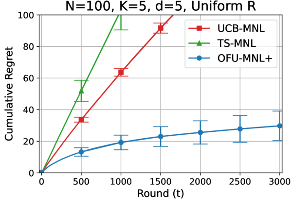
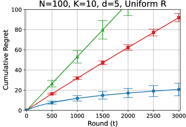
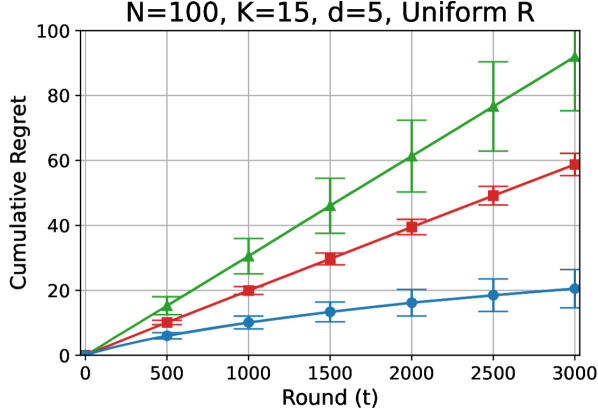
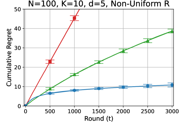
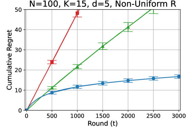
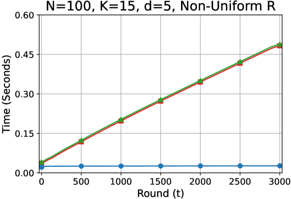
Figure 1: Cumulative regret (left three, $K=5,10,15$) and runtime per round (rightmost one, $K=15$) under uniform rewards (first row) and non-uniform rewards (second row) with $v_{0}=1$.

In this section, we empirically evaluate the performance of our algorithm OFU-MNL+. We measure cumulative regret over $T=3000$ rounds. For each experimental setup, we run the algorithms across $20$ independent instances and report the average performance. In each instance, the underlying parameter $\mathbf{w}^{\star}$ is randomly sampled from a $d$-dimensional uniform distribution, where each element of $\mathbf{w}^{\star}$ lies within the range $[-1/\sqrt{d},1/\sqrt{d}]$ and is not known to the algorithms. Additionally, the context features $x_{ti}$ are drawn from a $d$-dimensional multivariate Gaussian distribution, with each element of $x_{ti}$ clipped to the range $[-1/\sqrt{d},1/\sqrt{d}]$. This setup ensures compliance with Assumption 1. In the uniform reward setting (first row of Figure 1), the combinatorial optimization step to choose the assortment reduces to sorting items by their utility estimate. In the non-uniform reward setting (second row of Figure 1), the rewards are sampled from a uniform distribution in each round, i.e., $r_{ti}\sim\operatorname{Unif}(0,1)$. Refer Appendix I for more details.

We compare the performance of OFU-MNL+ with those of the practical and state-of-the-art algorithms: the Upper Confidence Bound-based algorithm, UCB-MNL [35], and the Thompson Sampling-based algorithm, TS-MNL [35]. Figure 1 demonstrates that our algorithm significantly outperforms other baseline algorithms. In the uniform reward setting, as $K$ increases, the cumulative regrets of all algorithms tend to decrease. In contrast, this trend is not observed in the non-uniform reward setting. Furthermore, the results also show that our algorithm maintains a constant computation cost per round, while the other algorithms exhibit a linear dependence on $t$. In Appendix I, we present the additional runtime curves (Figure I.1) as well as the regret curves of the other configuration where $v_{0}=\Theta(K)$ (Figure I.2). All of these empirical results align with our theoretical results.

7 Conclusion

In this paper, we propose minimax optimal lower and upper bounds for both uniform and non-uniform reward settings. We propose a computationally efficient algorithm, OFU-MNL+, that achieves a regret of $\tilde{\mathcal{O}}(d\sqrt{\smash[b]{T/K}})$ under uniform rewards and $\tilde{\mathcal{O}}(d\sqrt{T})$ under non-uniform rewards. We also prove matching lower bounds of $\Omega(d\sqrt{\smash[b]{T/K}})$ and $\Omega(d\sqrt{T})$ for each setting, respectively. Moreover, our empirical results support our theoretical findings, demonstrating that OFU-MNL+ is not only provably but also experimentally efficient.

Part Appendix

Appendix A Further Related Work

In this section, we discuss additional related works that complement Section 2. For simplicity, we consider only the dependence on the number of rounds $t$ for a computation cost in big-$\mathcal{O}$ notation.

Logistic Bandits. The logistic bandit model [20, 18, 3, 19] focuses on environments with binary rewards and explores the impact of non-linearity on the exploration-exploitation trade-off for parametrized bandits. The main research interest has been the algorithms’ dependence on the degree of non-linearity $\kappa$, which can grow exponentially in terms of the diameter of the decision domain $\mathcal{W}$. Zhang et al. [45] introduced the first efficient algorithm for binary logistic bandits with a $\mathcal{O}(1)$ computation cost, achieving a regret of $\tilde{\mathcal{O}}(d\sqrt{T}/\kappa)$. Faury et al. [18] enhanced the regret to $\tilde{\mathcal{O}}(d\sqrt{\smash[b]{T/\kappa}})$ with a $\mathcal{O}(t)$ computation cost. However, their regret bounds still suffered from a harmful dependence on $1/\kappa$. Abeille et al. [3] addressed this by achieving the tightest regret upper bound of $\tilde{\mathcal{O}}(d\sqrt{\kappa T})$ with a $\mathcal{O}(t)$ computation cost, while Faury et al. [19] achieved the same regret with an improved computation cost of $\mathcal{O}(\log t)$. More recently, Zhang and Sugiyama [47] proposed a jointly efficient algorithm that achieves the optimal regret with a constant $\mathcal{O}(1)$ computation cost. Note that the logistic bandit is a special case of the multinomial logistic (MNL) bandit. When the maximum assortment size is one ($K=1$), rewards are uniform ($r_{t1}=1$), and the utility for the outside option is one $v_{0}=1$, the MNL bandit reduces to the logistic bandit. In this logistic bandit setting, our proposed algorithm, OFU-MNL+, can achieve a regret upper bound of $\tilde{\mathcal{O}}(d\sqrt{\kappa T})$ with a constant $\mathcal{O}(1)$ computation cost, consistent with the result in Zhang and Sugiyama [47].

Multinomial Logistic (MNL) Bandits. There are two main approaches to multinomial logistic (MNL) bandits: the multiple-parameter choice model and the single-parameter choice model. In the multiple-parameter choice model, the learner estimates parameters for each choice in the assortment ($\mathbf{w}_{1}^{\star},\dots,\mathbf{w}_{K}^{\star}$) with a shared context $x_{t}$. In this setting, Amani and Thrampoulidis [8] proposed a feasible algorithm that achieves a regret upper bound of $\tilde{\mathcal{O}}(dK\sqrt{\kappa T})$ with a $\mathcal{O}(t)$ computation cost. They also proposed an intractable algorithm that achieves an improved regret of $\tilde{\mathcal{O}}(dK^{3/2}\sqrt{T})$. Zhang and Sugiyama [47] introduced a computationally and statistically efficient algorithm that obtains a regret of $\tilde{\mathcal{O}}(dK\sqrt{T})$. Recently, Lee et al. [29] further improved the regret by a factor of $\sqrt{K}$, achieving $\tilde{\mathcal{O}}(d\sqrt{KT})$ regret. In the multiple-parameter case, the regret’s dependence on $K$ is unavoidable since the number of unknown parameters depends on $K$.

On the other hand, the single-parameter choice model, closely related to ours, shares the parameter $\mathbf{w}^{\star}$ cross the choices, with varying contexts for each choice. The learner offers a set of items $S_{t}$, with $|S_{t}|\leq K$ at each round. This setting involves a combinatorial optimization to choose the assortment $S_{t}$, making it more challenging to devise a tractable algorithm. As extensively discussed in Section 2, no previous studies have definitively confirmed whether the existing lower or upper bounds are tight. As shown in Table 1, many studies have presented their results in inconsistent settings with varying reward structures and values of $v_{0}$, adding to the ambiguity about the bounds’ optimality. In this paper, we address these issues by bridging the gap between the lower and upper bounds of regret through a careful categorization of the settings. We propose an algorithm that is both provably optimal, up to logarithmic factors, and computationally efficient, significantly enhancing the theoretical and practical understanding of MNL bandits.

Generalized Linear Bandits. In generalized linear bandits [20, 23, 30, 2, 27, 24, 25], the expected rewards are modeled using a generalized linear model. These problems generalize logistic bandits by incorporating a general exponential family link function instead of the logistic link function. The algorithms proposed for generalized linear bandits also exhibit a dependence on the nonlinear term $\kappa$. However, our problem setting (single-parameter MNL bandits) considers a more complex state space where multiple arms are pulled simultaneously.

Combinatorial Bandits. Another related stream of literature is combinatorial bandits [11, 40, 26, 48, 41, 31], particularly top-$k$ combinatorial bandits [41]. In top-$k$ combinatorial bandits, the decision set includes all subsets of size $k$ out of $n$ arms, and the reward for each action is the sum of the rewards of the $k$ selected arms. In this framework, the rewards are assumed to be independent of the entire set of arms played in round $t$. In contrast, in our setting, the reward for each individual arm depends on the whole set of arms played.

Appendix B Notation

We denote $T$ as the total number of rounds and $t\in[T]$ as the current round. We denote $N$ as the total number of items, $K$ as the maximum size of assortments, and $d$ as the dimension of feature vectors.

For notational simplicity, we define the loss function in two different forms throughout the proof:

$$\ell_{t}(\mathbf{w}) =-\sum_{i\in S_{t}}y_{ti}\log p_{t}(i|S_{t},\mathbf{w})=-\sum_{i\in S_{t}}y_{ti}\log\left(\frac{\exp(x_{ti}^{\top}\mathbf{w})}{v_{0}\!+\!\sum_{j\in S_{t}}\exp(x_{tj}^{\top}\mathbf{w})}\right),$$

$$\ell(\mathbf{z}_{t},\mathbf{y}_{t}) =-\sum_{i\in S_{t}}y_{ti}\log\left(\frac{\exp(z_{ti})}{v_{0}\!+\!\sum_{j\in S_{t}}\exp(z_{tj})}\right),$$

where $z_{ti}=x_{ti}^{\top}\mathbf{w}$, $\mathbf{z}_{t}=(z_{ti})_{i\in S_{t}}\in\mathbb{R}^{|S_{t}|}$, and $\mathbf{y}_{t}=(y_{ti})_{i\in S_{t}}\in\mathbb{R}^{|S_{t}|}$. Thus, $\ell_{t}(\mathbf{w})=\ell(\mathbf{z}_{t},\mathbf{y}_{t})$.

We offer a Table B.1 for convenient reference.

Table B.1: Symbols

$x_{ti}$	feature vector for item $i$ given at round $t$
$r_{ti}$	reward for item $i$ given at round $t$
$S_{t}$	assortment chosen by an algorithm at round $t$
$0$	outside option
$y_{ti}$	choice response for each item $i\in S_{t}\cup\{0\}$ at round $t$
$R_{t}(S,\mathbf{w}^{\star})$	$:=\sum_{i\in S}p_{t}(i|S,\mathbf{w}^{\star})r_{ti}$, expected revenue of the assortment $S$ at round $t$
$\ell_{t}(\mathbf{w})$	$:=-\sum_{i\in S_{t}}y_{ti}\log\left(\frac{\exp(x_{ti}^{\top}\mathbf{w})}{v_{0}\!+\!\sum_{j\in S_{t}}\exp(x_{tj}^{\top}\mathbf{w})}\right)$, loss function at round $t$
$\ell(\mathbf{z}_{t},\mathbf{y}_{t})$	$:=-\sum_{i\in S_{t}}y_{ti}\log\left(\frac{\exp(z_{ti})}{v_{0}\!+\!\sum_{j\in S_{t}}\exp(z_{tj})}\right)$, loss function at round $t$, $z_{ti}=x_{ti}^{\top}\mathbf{w}$
$\lambda$	regularization parameter
$\mathcal{G}_{t}(\mathbf{w})$	$:=\sum_{i\in S_{t}}p_{t}(i|S_{t},\mathbf{w})x_{ti}x_{ti}^{\top}-\sum_{i\in S_{t}}\sum_{j\in S_{t}}p_{t}(i|S_{t},\mathbf{w})p_{t}(j|S_{t},\mathbf{w})x_{ti}x_{tj}^{\top}$
$H_{t}$	$:=\lambda\mathbf{I}_{d}+\sum_{s=1}^{t-1}\mathcal{G}_{s}(\mathbf{w}_{s+1})$
$\tilde{H}_{t}$	$:=H_{t}+\eta\mathcal{G}_{t}(\mathbf{w}_{t})$
$\alpha_{ti}$	$:=x_{ti}^{\top}\mathbf{w}_{t}+\beta_{t}(\delta)\|x_{ti}\|_{H_{t}^{-1}}$, optimistic utility for item $i$ at round $t$
$\beta_{t}(\delta)$	$:=\mathcal{O}\left(\sqrt{d}\log t\log K\right)$, confidence radius at round $t$
$\tilde{R}_{t}(S)$	$:=\frac{\sum_{i\in S}\exp(\alpha_{ti})r_{ti}}{v_{0}+\sum_{j\in S}\exp(\alpha_{ti})}$, optimistic expected revenue for the assortment $S$ at round $t$

Appendix C Properties of MNL function

In this section, we present key properties of the MNL function and its associated loss, which are used throughout the paper.

C.1 Utility for Outside Option: $v_{0}=\Theta(1)$ is Common in Contextual MNL Bandits

In this subsection, we explain why the assumption that $v_{0}=\Theta(1)$ is made without loss of generality. Let the original feature vectors be $x^{\prime}_{ti}\in\mathbb{R}^{d}$ for every item $i\in[N]$. Suppose that a context for the outside option $x_{t0}^{\prime}$ is given and the probability of choosing any item $i\in S_{t}\cup\{0\}$ is defined as

$$p_{t}(i|S_{t},\mathbf{w}^{\star})=\frac{\exp((x^{\prime}_{ti})^{\top}\mathbf{w}^{\star})}{\sum_{j\in S_{t}\cup\{0\}}\exp((x^{\prime}_{tj})^{\top}\mathbf{w}^{\star})}.$$

Then, by dividing the denominator and numerator by $\exp\left((x^{\prime}_{t0})^{\top}\mathbf{w}^{\star}\right)$, and defining $x_{ti}:=x^{\prime}_{ti}-x^{\prime}_{t0}$, we obtain the MNL probability in the form presented in (1) with $v_{0}=\exp(0)=1$. Note that this division does not change the probability. Therefore, $v_{0}=\Theta(1)$ is natural and common in contextual MNL bandit literature.

C.2 Self-concordant-like Function

Definition C.1 (Self-concordant-like function, Tran-Dinh et al. 44).

A convex function $f\in\mathcal{C}^{3}(\mathbb{R}^{m})$ is $M$-self-concordant-like function with constant $M$ if:

$$|\phi^{\prime\prime\prime}(s)|\leq M\|\mathbf{b}\|_{2}\phi^{\prime\prime}(s).$$

for $s\in\mathbb{R}$ and $M>0$, where $\phi(s):=f(\mathbf{a}+s\mathbf{b})$ for any $\mathbf{a},\mathbf{b}\in\mathbb{R}^{m}$.

Then, the MNL loss defined in (2) is $3\sqrt{2}$-self-concordant-like function.

Proposition C.1.

For any $t\in[T]$, the multinomial logistic loss $\ell_{t}(\mathbf{w})$, defined in (2), is $3\sqrt{2}$-self-concordant-like.

Proof.

Consider the function $\phi(s):=\log\left(\sum_{i=0}^{n}e^{a_{i}s+b_{i}}\right)$, where $\mathbf{a}=[a_{0},\dots,a_{n}]^{\top}\in\mathbb{R}^{n+1}$ and $\mathbf{b}=[b_{0},\dots,b_{n}]^{\top}\in\mathbb{R}^{n+1}$. Then, by simple calculus, we have

$$\phi^{\prime\prime}(s)=\frac{\sum_{i<j}(a_{i}-a_{j})^{2}e^{a_{i}s+b_{i}}e^{a_{j}s+b_{j}}}{\left(\sum_{i=0}^{n}e^{a_{i}s+b_{i}}\right)^{2}}\geq 0,$$

and

$$\phi^{\prime\prime\prime}(s)=\frac{\sum_{i<j}(a_{i}-a_{j})^{2}e^{a_{i}s+b_{i}}e^{a_{j}s+b_{j}}\left[\sum_{k=0}^{n}(a_{i}+a_{j}-2a_{k})e^{a_{k}s+b_{k}}\right]}{\left(\sum_{i=0}^{n}e^{a_{i}s+b_{i}}\right)^{3}}.$$ (C.1)

Note that for all $i,j,k=0,\dots,n$,

$$|a_{i}+a_{j}-2a_{k}|\leq\sqrt{6}\sqrt{a_{i}^{2}+a_{j}^{2}+a_{k}^{2}}\leq 3\sqrt{2}\max_{i=0,\dots,n}|a_{i}|.$$ (C.2)

Therefore, we have

$$\left|\sum_{k=0}^{n}(a_{i}+a_{j}-2a_{k})e^{a_{k}s+b_{k}}\right|\leq\sum_{k=0}^{n}\left|a_{i}+a_{j}-2a_{k}\right|e^{a_{k}s+b_{k}}\leq 3\sqrt{2}\max_{i=0,\dots,n}|a_{i}|\sum_{k=0}^{n}e^{a_{k}s+b_{k}}.$$ (C.3)

Plugging in (C.3) into (C.1), we obtain

$$\phi^{\prime\prime\prime}(s)\leq 3\sqrt{2}\max_{i=0,\dots,n}|a_{i}|\phi^{\prime\prime}(s).$$ (C.4)

Now, we are ready to prove the proposition. For any $t\in[T]$, let $n=|S_{t}|$ and $c_{1}=x_{ti_{1}},c_{2}=x_{ti_{2}},\dots,c_{n}=x_{ti_{n}}$. Define a function $f\in\mathcal{C}^{3}:\mathbb{R}^{d}\rightarrow\ \mathbb{R}$ as $f(\bm{\theta}):=\log\left(v_{0}+\sum_{i=1}^{n}e^{c_{i}^{\top}\bm{\theta}}\right)$. Let $\bm{\delta}\in\mathbb{R}^{d}$ and let $f(\bm{\theta}+s\bm{\delta})=\log\left(v_{0}+\sum_{i=1}^{n}e^{c_{i}^{\top}\bm{\theta}+sc_{i}^{\top}\bm{\delta}}\right)=\log\left(\sum_{i=0}^{n}e^{a_{i}s+b_{i}}\right)=\phi(s)$, where $a_{i}=c_{i}^{\top}\bm{\delta}$, $b_{i}=c_{i}^{\top}\bm{\theta}$ for $i=1,\dots,n$, and $a_{i}=0$ and $b_{i}=\log v_{0}$ for $i=0$. Then, by (C.4), we get

$$|\phi^{\prime\prime\prime}(s)| \leq 3\sqrt{2}\max_{i=0,\dots,n}|a_{i}|\phi^{\prime\prime}(s)=3\sqrt{2}\max_{i=1,\dots,n}|c_{i}^{\top}\bm{\delta}|\phi^{\prime\prime}(s)$$

$$\leq 3\sqrt{2}\max_{i=1,\dots,n}\|c_{i}\|_{2}\|\bm{\delta}\|_{2}\phi^{\prime\prime}(s)\leq 3\sqrt{2}\|\bm{\delta}\|_{2}\phi^{\prime\prime}(s),$$

where the last inequality holds due to Assumption  1 that $\|c_{i}\|_{2}=\|x_{tj_{i}}\|_{2}\leq 1$. Then, by Definition C.1, $f$ is $3\sqrt{2}$-self-concordant-like. Since $\ell_{t}$ is the sum of $f$ and a linear operator, which has third derivatives equal to zero, it follows that $\ell_{t}$ is also $3\sqrt{2}$-self-concordant-like function. ∎

Remark C.1.

Contrary to the findings of Perivier and Goyal [39], which suggest that the MNL loss function $\sqrt{6K}$-self-concordant-like, our loss function is $3\sqrt{2}$-self-concordant-like. This yields an improved regret bound on the order of $\mathcal{O}(\sqrt{K})$. The improvement arises due to a $K$-independent self-concordant-like property of $\ell_{t}$, as shown in Proposition C.1. In Perivier and Goyal [39], Lemma 4 from  Tran-Dinh et al. [44] is used, which describes a $\sqrt{6}\|\mathbf{a}\|_{2}$ self-concordant-like property. However, in the analysis of C.2, we show that their analysis is not tight because they bound the term $\sqrt{\smash[b]{a_{i}^{2}+a_{j}^{2}+a_{k}^{2}}}$ by $\|\mathbf{a}\|_{2}=\sqrt{\sum_{i=0}^{n}a_{i}^{2}}$, thus making its upper bound dependent on $K$, i.e., $n=|S_{t}|\leq K$. In contrast, we bound the same term by a constant, $\max_{i=1,\dots,n}\|a_{i}\|_{2}$, which allows our loss function to exhibit a constant $3\sqrt{2}$-self-concordant-like property. This key difference accounts for the $\sqrt{K}$-improved regret.

Lemma C.1 (Theorem 3 of Tran-Dinh et al. 44).

A convex function $\ell\in\mathcal{C}^{3}:\mathbb{R}^{d}\rightarrow\mathbb{R}$ is $M$-self-concordant-like if and only if for any $\mathbf{v},\mathbf{u}_{1},\mathbf{u}_{2},\mathbf{u}_{3}\in\mathbb{R}^{d}$, we have

$$|\langle D^{3}\ell(\mathbf{v})[\mathbf{u}_{1}]\mathbf{u}_{2},\mathbf{u}_{3}\rangle|\leq M\|\mathbf{u}_{1}\|_{2}\|\mathbf{u}_{2}\|_{\nabla^{2}\ell(\mathbf{v})}\|\mathbf{u}_{3}\|_{\nabla^{2}\ell(\mathbf{v})}.$$

Appendix D Proof of Theorem 1

In this section, we provide the proof of Theorem 1. The proof structure is similar to the one presented in Chen et al. [13]. However, unlike their approach, we explicitly derive a bound that includes $v_{0}$. Furthermore, by establishing a tighter upper bound for the KL divergence (Lemma D.2), we derive a bound that is tighter than the one provided by Chen et al. [13].

D.1 Adversarial Construction and Bayes Risk

Let $\epsilon\in(0,1/d\sqrt{d})$ be a small positive parameter to be specified later. For every subset $V\subseteq[d]$, we define the corresponding parameter $\mathbf{w}_{V}\in\mathbb{R}^{d}$ as $[\mathbf{w}_{V}]_{j}=\epsilon$ for all $j\in V$, and $[\mathbf{w}_{V}]_{j}=0$ for all $j\notin V$. Then, we consider the following parameter set

$$\mathbf{w}\in\mathcal{W}:=\{\mathbf{w}_{V}:V\in\mathcal{V}_{d/4}\}:=\{\mathbf{w}_{V}:V\subseteq[d],|V|=d/4\},$$

where $\mathcal{V}_{k}$ denotes the class of all subsets of $[d]$ whose size is $k$. Moreover, note that $d/4$ is a positive integer, as $d$ is divisible by $4$ by construction.

The context vectors $\{x_{ti}\}$ are constructed to be invariant across rounds $t$. For each $t$ and $U\in\mathcal{V}_{d/4}$, $K$ identical context vectors  $x_{U}$ are constructed as follows:

$$[x_{U}]_{j}=1/\sqrt{d}\quad\text{for}\,\,j\in U;\quad[x_{U}]_{j}=0\quad\text{for}\,\,j\notin U.$$

For all $V,U\in\mathcal{V}_{d/4}$, it can be verified that $\mathbf{w}_{V}$ and $x_{U}$ satisfy the requirements of a bounded assumption 1 as follows:

$$\|\mathbf{w}_{V}\|_{2}\leq\sqrt{d\epsilon^{2}}\leq 1,\quad\|x_{U}\|_{2}\leq\sqrt{d\cdot 1/d}=1.$$

Therefore, the worst-case expected regret of any policy $\pi$ can be lower bounded by the worst-case expected regret of parameters belonging to $\mathcal{W}$, which can be further lower bounded by the “average” regret over a uniform prior over $\mathcal{W}$ as follows:

$$\sup_{\mathbf{w}}\mathbb{E}_{\mathbf{w}}^{\pi}\left[\textup{{Reg}}_{T}(\mathbf{w})\right] =\sup_{\mathbf{w}}\mathbb{E}_{\mathbf{w}}^{\pi}\sum_{t=1}^{T}R(S^{\star},\mathbf{w})-R(S_{t},\mathbf{w})$$

$$\geq\max_{\mathbf{w}_{V}\in\mathcal{W}}\mathbb{E}_{\mathbf{w}_{V}}^{\pi}\sum_{t=1}^{T}R(S^{\star},\mathbf{w}_{V})-R(S_{t},\mathbf{w}_{V})$$

$$\geq\frac{1}{|\mathcal{V}_{d/4}|}\sum_{V\in\mathcal{V}_{d/4}}\mathbb{E}_{\mathbf{w}_{V}}^{\pi}\sum_{t=1}^{T}R(S^{\star},\mathbf{w}_{V})-R(S_{t},\mathbf{w}_{V})$$

$$=\frac{1}{|\mathcal{V}_{d/4}|}\sum_{V\in\mathcal{V}_{d/4}}\mathbb{E}_{\mathbf{w}_{V}}^{\pi}\sum_{t=1}^{T}\left[\sum_{i\in S^{\star}}p(i|S^{\star},\mathbf{w}_{V})-\sum_{i\in S_{t}}p(i|S_{t},\mathbf{w}_{V})\right].$$ (D.1)

This reduces the task of lower bounding the worst-case regret of any policy to the task of lower bounding the Bayes risk of the constructed parameter set.

D.2 Main Proof of Theorem 1

Proof of Theorem 1.

For any sequence of assortments $\{S_{t}\}_{t=1}^{T}$ produced by policy $\pi$, we denote an alternative sequence $\{\tilde{S}_{t}\}_{t=1}^{T}$ that provably enjoys less regret under parameterization $\mathbf{w}_{V}$.

Let $x_{U_{1}},\dots,x_{U_{L}}$ be the distinct feature vectors contained in assortments $S_{t}$ (if $S_{t}=\emptyset$, then one may choose an arbitrary feature $x_{U}$) with $U_{1},\dots,U_{L}\in\mathcal{V}_{d/4}$. Let $U^{\star}$ be the subset among $U_{1},\dots,U_{L}$ that maximizes $x_{U}^{\top}\mathbf{w}_{V}$, i.e., $U^{\star}\in\mathop{\mathrm{argmax}}_{U\in\{U_{1},\dots,U_{L}\}}x_{U}^{\top}\mathbf{w}_{V}$, where $\mathbf{w}_{V}$ is the underlying parameter. Then, we define $\tilde{S}_{t}$ as the assortment consisting of all $K$ items corresponding to feature $x_{U^{\star}}$, i.e., $\tilde{S}_{t}=\{\underbrace{x_{U^{\star}},\dots,x_{U^{\star}}}_{K}\}$.

Since the expected revenue is an increasing function, we have the following observation:

Proposition D.1 (Proposition 1 in Chen et al. 13).

$$\sum_{i\in S_{t}}p(i|S_{t},\mathbf{w}_{V})\leq\sum_{i\in\tilde{S}_{t}}p(i|\tilde{S}_{t},\mathbf{w}_{V}).$$

Proposition D.1 implies that $\sum_{i\in S^{\star}}p(i|S^{\star},\mathbf{w}_{V})-\sum_{i\in S_{t}}p(i|S_{t},\mathbf{w}_{V})\geq\sum_{i\in S^{\star}}p(i|S^{\star},\mathbf{w}_{V})-\sum_{i\in\tilde{S}_{t}}p(i|\tilde{S}_{t},\mathbf{w}_{V})$. Hence, it is sufficient to bound $\sum_{i\in S^{\star}}p(i|S^{\star},\mathbf{w}_{V})-\sum_{i\in\tilde{S}_{t}}p(i|\tilde{S}_{t},\mathbf{w}_{V})$ instead of $\sum_{i\in S^{\star}}p(i|S^{\star},\mathbf{w}_{V})-\sum_{i\in S_{t}}p(i|S_{t},\mathbf{w}_{V})$.

To simplify notation, we denote $\tilde{U}_{t}$ as the unique $U^{\star}\in\mathcal{V}_{d/4}$ in $\tilde{S}_{t}$. We also use $\mathbb{E}_{V}$ and $\mathbb{P}_{V}$ to denote the expected value and probability, respectively, as governed by the law parameterized by $\mathbf{w}_{V}$ and under policy $\pi$. Then, we can establish a lower bound for $\sum_{i\in S^{\star}}p(i|S^{\star},\mathbf{w}_{V})-\sum_{i\in\tilde{S}_{t}}p(i|\tilde{S}_{t},\mathbf{w}_{V})$ as follows:

Lemma D.1.

Suppose $\epsilon\in(0,1/d\sqrt{d})$ and define $\delta:=d/4-|\tilde{U}_{t}\cap V|$. Then, we have

$$\sum_{i\in S^{\star}}p(i|S^{\star},\mathbf{w}_{V})-\sum_{i\in\tilde{S}_{t}}p(i|\tilde{S}_{t},\mathbf{w}_{V})\geq\frac{v_{0}K}{(v_{0}+Ke)^{2}}\cdot\frac{\delta\epsilon}{2\sqrt{d}}.$$

For any $j\in V$, define random variables $\tilde{M}_{j}:=\sum_{t=1}^{T}\mathbf{1}\{j\in\tilde{U}_{t}\}$. Then, by Lemma D.1, for all $V\in\mathcal{V}_{d/4}$, we have

$$\mathbb{E}_{V}\sum_{i\in S^{\star}}p(i|S^{\star},\mathbf{w}_{V})-\sum_{i\in\tilde{S}_{t}}p(i|\tilde{S}_{t},\mathbf{w}_{V})\geq\frac{v_{0}K}{(v_{0}+Ke)^{2}}\cdot\frac{\epsilon}{2\sqrt{d}}\left(\frac{dT}{4}-\sum_{j\in V}\mathbb{E}_{V}[\tilde{M}_{j}]\right).$$ (D.2)

Furthermore, we define $\mathcal{V}_{d/4}^{(j)}:=\{V\in\mathcal{V}_{d/4}:j\in V\}$ and $\mathcal{V}_{d/4-1}:=\{V\subseteq[d]:|V|=d/4-1\}$. By taking the average of both sides of Equation (D.2) with respect to all $V\in\mathcal{V}_{d/4}$, we obtain

$$\frac{1}{\left|\mathcal{V}_{d/4}\right|}\sum_{V\in\mathcal{V}_{d/4}}\mathbb{E}_{V}\sum_{i\in S^{\star}}p(i|S^{\star},\mathbf{w}_{V})-\sum_{i\in\tilde{S}_{t}}p(i|\tilde{S}_{t},\mathbf{w}_{V})$$

$$\geq\frac{v_{0}K}{(v_{0}+Ke)^{2}}\cdot\frac{\epsilon}{2\sqrt{d}}\cdot\frac{1}{\left|\mathcal{V}_{d/4}\right|}\sum_{V\in\mathcal{V}_{d/4}}\left(\frac{dT}{4}-\sum_{j\in V}\mathbb{E}_{V}[\tilde{M}_{j}]\right)$$

$$=\frac{v_{0}K}{(v_{0}+Ke)^{2}}\cdot\frac{\epsilon}{2\sqrt{d}}\left(\frac{dT}{4}-\frac{1}{\left|\mathcal{V}_{d/4}\right|}\sum_{j=1}^{d}\sum_{V\in\mathcal{V}_{d/4}^{(j)}}\mathbb{E}_{V}[\tilde{M}_{j}]\right)$$

$$=\frac{v_{0}K}{(v_{0}+Ke)^{2}}\cdot\frac{\epsilon}{2\sqrt{d}}\left(\frac{dT}{4}-\frac{1}{\left|\mathcal{V}_{d/4}\right|}\sum_{V\in\mathcal{V}_{d/4-1}}\sum_{j\notin V}\mathbb{E}_{V\cup\{j\}}[\tilde{M}_{j}]\right)$$

$$\geq\frac{v_{0}K}{(v_{0}+Ke)^{2}}\cdot\frac{\epsilon}{2\sqrt{d}}\left(\frac{dT}{4}-\frac{\left|\mathcal{V}_{d/4-1}\right|}{\left|\mathcal{V}_{d/4}\right|}\max_{V\in\mathcal{V}_{d/4-1}}\sum_{j\notin V}\mathbb{E}_{V\cup\{j\}}[\tilde{M}_{j}]\right)$$

$$=\frac{v_{0}K}{(v_{0}+Ke)^{2}}\cdot\frac{\epsilon}{2\sqrt{d}}\left(\frac{dT}{4}-\frac{\left|\mathcal{V}_{d/4-1}\right|}{\left|\mathcal{V}_{d/4}\right|}\max_{V\in\mathcal{V}_{d/4-1}}\sum_{j\notin V}\mathbb{E}_{V}[\tilde{M}_{j}]+\mathbb{E}_{V\cup\{j\}}[\tilde{M}_{j}]-\mathbb{E}_{V}[\tilde{M}_{j}]\right).$$

For any fixed $V$, we get $\sum_{j\notin V}\mathbb{E}_{V}[\tilde{M}_{j}]\leq\sum_{j=1}^{d}\mathbb{E}_{V}[\tilde{M}_{j}]\leq dT/4$. Also, we have $\frac{\left|\mathcal{V}_{d/4-1}\right|}{\left|\mathcal{V}_{d/4}\right|}=\binom{d}{d/4-1}/\binom{d}{d/4}=\frac{d/4}{3d/4+1}\leq\frac{1}{3}$. Consequently, we derive that

$$\frac{1}{\left|\mathcal{V}_{d/4}\right|} \sum_{V\in\mathcal{V}_{d/4}}\mathbb{E}_{V}\sum_{i\in S^{\star}}p(i|S^{\star},\mathbf{w}_{V})-\sum_{i\in\tilde{S}_{t}}p(i|\tilde{S}_{t},\mathbf{w}_{V})$$

$$\geq\frac{v_{0}K}{(v_{0}+Ke)^{2}}\cdot\frac{\epsilon}{2\sqrt{d}}\left(\frac{dT}{6}-\max_{V\in\mathcal{V}_{d/4-1}}\sum_{j\notin V}\left|\mathbb{E}_{V\cup\{j\}}[\tilde{M}_{j}]-\mathbb{E}_{V}[\tilde{M}_{j}]\right|\right).$$ (D.3)

Now we bound the term $\left|\mathbb{E}_{V\cup\{j\}}[\tilde{M}_{j}]-\mathbb{E}_{V}[\tilde{M}_{j}]\right|$ in (D.3) for any $V\in\mathcal{V}_{d/4-1}$. For simplicity, let $P=\mathbb{P}_{V}$ and $Q=\mathbb{P}_{V\cup\{j\}}$ denote the laws under $\mathbf{w}_{V}$ and $\mathbf{w}_{V\cup j}$, respectively. Then, we have

$$\left|\mathbb{E}_{P}[\tilde{M}_{j}]-\mathbb{E}_{Q}[\tilde{M}_{j}\right]| \leq\sum_{t=0}^{T}t\cdot\left|P[\tilde{M}_{j}=t]-Q[\tilde{M}_{j}=t]\right|$$

$$\leq T\cdot\sum_{t=0}^{T}\left|P[\tilde{M}_{j}=t]-Q[\tilde{M}_{j}=t]\right|$$

$$\leq T\cdot\|P-Q\|_{\operatorname{TV}}\leq T\cdot\sqrt{\frac{1}{2}\operatorname{KL}(P\|Q)},$$ (D.4)

where $\|P-Q\|_{\operatorname{TV}}=\sup_{A}|P(A)-Q(A)|$ | is the total variation distance between $P$ and $Q$, $\operatorname{KL}(P\|Q)=\int(\log\mathrm{d}P/\mathrm{d}Q)\mathrm{d}P$ is s the Kullback-Leibler (KL) divergence between $P$ and $Q$, and the last inequality holds by Pinsker’s inequality. Now, we bound the KL divergence term using the following Lemma.

Lemma D.2.

For any $V\in\mathcal{V}_{d/4-1}$ and $j\in[d]$, there exists a positive constant $C_{\operatorname{KL}}>0$ such that

$$\operatorname{KL}(P_{V}\|Q_{V\cup\{j\}})\leq C_{\operatorname{KL}}\cdot\frac{v_{0}K}{(v_{0}+K)^{2}}\cdot\frac{\mathbb{E}_{V}[\tilde{M}_{j}]\epsilon^{2}}{d}.$$

Therefore, combining (D.3), (D.4), and Lemma D.2, we have

$$\frac{1}{\left|\mathcal{V}_{d/4}\right|} \sum_{V\in\mathcal{V}_{d/4}}\mathbb{E}_{V}\sum_{i\in S^{\star}}p(i|S^{\star},\mathbf{w}_{V})-\sum_{i\in\tilde{S}_{t}}p(i|\tilde{S}_{t},\mathbf{w}_{V})$$

$$\geq\frac{v_{0}K}{(v_{0}+Ke)^{2}}\cdot\frac{\epsilon}{2\sqrt{d}}\left(\frac{dT}{6}-T\sum_{j=1}^{d}\sqrt{C_{\operatorname{KL}}\cdot\frac{v_{0}K}{(v_{0}+K)^{2}}\cdot\frac{\mathbb{E}_{V}[\tilde{M}_{j}]\epsilon^{2}}{d}}\right)$$

$$\geq\frac{v_{0}K}{(v_{0}+Ke)^{2}}\cdot\frac{\epsilon}{2\sqrt{d}}\left(\frac{dT}{6}-T\sqrt{d}\cdot\sqrt{\sum_{j=1}^{d}C_{\operatorname{KL}}\cdot\frac{v_{0}K}{(v_{0}+K)^{2}}\cdot\frac{\mathbb{E}_{V}[\tilde{M}_{j}]\epsilon^{2}}{d}}\right)$$

$$\geq\frac{v_{0}K}{(v_{0}+Ke)^{2}}\cdot\frac{\epsilon}{2\sqrt{d}}\left(\frac{dT}{6}-T\sqrt{d}\cdot\sqrt{\frac{C_{\operatorname{KL}}}{4}\cdot\frac{v_{0}K}{(v_{0}+K)^{2}}\cdot T\epsilon^{2}}\right),$$

where the second inequality is due to the Cauchy-Schwartz inequality and the last inequality holds because $\sum_{j=1}^{d}\mathbb{E}_{V}[\tilde{M}_{j}]\leq dT/4$. Let $C_{\operatorname{KL}}^{\prime}=C_{\operatorname{KL}}/4$.

By setting $\epsilon=\sqrt{\frac{d}{144C_{\operatorname{KL}}^{\prime}T}\cdot\frac{(v_{0}+K)^{2}}{v_{0}K}}$, we have

$$\sup_{\mathbf{w}}\mathbb{E}_{\mathbf{w}}^{\pi}\left[\textup{{Reg}}_{T}(\mathbf{w})\right] \geq\frac{v_{0}K}{(v_{0}+Ke)^{2}}\cdot\frac{\epsilon}{2\sqrt{d}}\left(\frac{dT}{6}-\sqrt{C_{\operatorname{KL}}^{\prime}\cdot\frac{v_{0}K}{(v_{0}+K)^{2}}dT\epsilon^{2}}\right)$$

$$=\frac{v_{0}K}{(v_{0}+Ke)^{2}}\cdot\sqrt{\frac{(v_{0}+K)^{2}}{v_{0}K}}\cdot\frac{1}{288\sqrt{C_{\operatorname{KL}}^{\prime}}}d\sqrt{T}$$

$$=\Omega\left(\frac{\sqrt{v_{0}K}}{v_{0}+K}\cdot d\sqrt{T}\right).$$

This concludes the proof of Theorem 1. ∎

D.3 Proofs of Lemmas for Theorem 1

D.3.1 Proof of Lemma D.1

Proof of Lemma D.1.

Let $x=x_{V}$ and $\hat{x}=x_{\tilde{U}_{t}}$ be the corresponding context vectors. Then, we have

$$\sum_{i\in S^{\star}}p(i|S^{\star},\mathbf{w}_{V})-\sum_{i\in\tilde{S}_{t}}p(i|\tilde{S}_{t},\mathbf{w}_{V}) =\frac{K\exp\left(x^{\top}\mathbf{w}_{V}\right)}{v_{0}+K\exp\left(x^{\top}\mathbf{w}_{V}\right)}-\frac{K\exp\left(\hat{x}^{\top}\mathbf{w}_{V}\right)}{v_{0}+K\exp\left(\hat{x}^{\top}\mathbf{w}_{V}\right)}$$

$$=\frac{v_{0}K\left(\exp\left(x^{\top}\mathbf{w}_{V}\right)-\exp\left(\hat{x}^{\top}\mathbf{w}_{V}\right)\right)}{\left(v_{0}+K\exp\left(x^{\top}\mathbf{w}_{V}\right)\right)\left(v_{0}+\exp\left(\hat{x}^{\top}\mathbf{w}_{V}\right)\right)}$$

$$\geq\frac{v_{0}K\left(\exp\left(x^{\top}\mathbf{w}_{V}\right)-\exp\left(\hat{x}^{\top}\mathbf{w}_{V}\right)\right)}{(v_{0}+Ke)^{2}},$$ (D.5)

where the inequality holds since $\max\left\{\exp\left(x^{\top}\mathbf{w}_{V}\right),\exp\left(\hat{x}^{\top}\mathbf{w}_{V}\right)\right\}\leq e$. To further bound the right-hand side of  (D.5), we use the fact that $1+a\leq e^{a}\leq 1+a+a^{2}/2$ for all $a\in[0,1]$, which can be easily shown by Taylor expansion. Thus, we get

$$\sum_{i\in S^{\star}}p(i|S^{\star},\mathbf{w}_{V})-\sum_{i\in\tilde{S}_{t}}p(i|\tilde{S}_{t},\mathbf{w}_{V}) \geq\frac{v_{0}K\left((x-\hat{x})^{\top}\mathbf{w}_{V}-(\hat{x}^{\top}\mathbf{w}_{V})^{2}/2\right)}{(v_{0}+Ke)^{2}}$$

$$\geq\frac{v_{0}K\left(\delta\epsilon/\sqrt{d}-(\sqrt{d}\epsilon)^{2}/2\right)}{(v_{0}+Ke)^{2}}$$

$$\geq\frac{v_{0}K\delta\epsilon}{2\sqrt{d}(v_{0}+Ke)^{2}},$$

where the last inequality holds because $(\sqrt{d}\epsilon)^{2}\leq\delta\epsilon/\sqrt{d}$ when $\epsilon\in(0,1/d\sqrt{d})$. This concludes the proof. ∎

D.3.2 Proof of Lemma D.2

Proof of Lemma D.2.

Fix a round $t$, an assortment $\tilde{S}_{t}$, and $\tilde{U}_{t}$. Let $U=\tilde{U}_{t}$. Define $m_{j}(\tilde{S}_{t}):=\sum_{x_{U}\in\tilde{S}_{t}}\mathbf{1}\{j\in U\}/K$. Let $\{p_{i}\}_{i\in\tilde{S}_{t}\cup\{0\}}$ and $\{q_{i}\}_{i\in\tilde{S}_{t}\cup\{0\}}$ be the probabilities of choosing item $i$ under parameterization $\mathbf{w}_{V}$ and $\mathbf{w}_{V\cup\{j\}}$, respectively. Then, we have

$$\operatorname{KL}\left(P_{V}(\cdot|\tilde{S}_{t})\|P_{V\cup\{j\}}(\cdot|\tilde{S}_{t})\right)=\sum_{i\in\tilde{S}_{t}\cup\{0\}}p_{i}\log\frac{p_{i}}{q_{i}}\leq\sum_{i\in\tilde{S}_{t}\cup\{0\}}p_{i}\frac{p_{i}-q_{i}}{q_{i}}\leq\sum_{i\in\tilde{S}_{t}\cup\{0\}}\frac{(p_{i}-q_{i})^{2}}{q_{i}},$$

where the first inequality holds because $\log(1+x)\leq x$ for all $x>-1$.

Let $\hat{x}=x_{U}$. Now, we separately upper bound $(p_{i}-q_{i})^{2}/q_{i}$, by analyzing the following three cases:

Case 1. The outside option, $i=0$.

For $i=0$, $q_{i}\geq\frac{v_{0}}{v_{0}+Ke}$. Thus, we have

$$|p_{i}-q_{i}| =\left|\frac{v_{0}}{v_{0}+\sum_{i\in\tilde{S}_{t}}\exp\left(x_{i}^{\top}\mathbf{w}_{V}\right)}-\frac{v_{0}}{v_{0}+\sum_{i\in\tilde{S}_{t}}\exp\left(x_{i}^{\top}\mathbf{w}_{V\cup\{j\}}\right)}\right|$$

$$=\left|\frac{v_{0}}{v_{0}+K\exp\left(\hat{x}^{\top}\mathbf{w}_{V}\right)}-\frac{v_{0}}{v_{0}+K\exp\left(\hat{x}^{\top}\mathbf{w}_{V\cup\{j\}}\right)}\right|$$

$$\leq\frac{v_{0}K}{(v_{0}+K/e)^{2}}\left|\exp\left(\hat{x}^{\top}\mathbf{w}_{V}\right)-\exp\left(\hat{x}^{\top}\mathbf{w}_{V\cup\{j\}}\right)\right|$$

$$=\frac{v_{0}K}{(v_{0}+K/e)^{2}}\left|e^{\bar{c}_{1}}(\hat{x}^{\top}\mathbf{w}_{V}-\hat{x}^{\top}\mathbf{w}_{V\cup\{j\}})\right|$$

$$\leq\frac{v_{0}Ke}{(v_{0}+K/e)^{2}}\left|\hat{x}^{\top}\left(\mathbf{w}_{V}-\mathbf{w}_{V\cup\{j\}}\right)\right|\leq\frac{v_{0}Ke}{(v_{0}+K/e)^{2}}\cdot\frac{m_{j}(\tilde{S}_{t})\epsilon}{\sqrt{d}},$$

where the third equality holds by applying the mean value theorem for the exponential function, with $\bar{c}_{1}:=(1-u)(\hat{x}^{\top}\mathbf{w}_{V})+u(\hat{x}^{\top}\mathbf{w}_{V\cup\{j\}})$ for some $u\in(0,1)$. Then, there exist an absolute constant $C_{0}$ such that

$$\frac{(p_{0}-q_{0})^{2}}{q_{0}} \leq\frac{v_{0}^{2}K^{2}e^{2}}{(v_{0}+K/e)^{4}}\cdot\frac{\left(m_{j}(\tilde{S}_{t})\right)^{2}\epsilon^{2}}{d}\cdot\frac{v_{0}+Ke}{v_{0}}$$

$$\leq C_{0}\cdot\frac{v_{0}K^{2}}{(v_{0}+K)^{3}}\cdot\frac{m_{j}(\tilde{S}_{t})\epsilon^{2}}{d},$$ (D.6)

where the last inequality holds since $m_{j}(\tilde{S}_{t})\leq 1$.

Case 2. $i\in\tilde{S}_{t}$ and $j\notin U$.

Then, for any $i\in\tilde{S}_{t}$ corresponding to $x_{i}=\hat{x}$ and $j\notin U$, we have

$$|p_{i}-q_{i}| =\left|\frac{\exp\left(\hat{x}^{\top}\mathbf{w}_{V}\right)}{v_{0}+K\exp\left(\hat{x}^{\top}\mathbf{w}_{V}\right)}-\frac{\exp\left(\hat{x}^{\top}\mathbf{w}_{V\cup\{j\}}\right)}{v_{0}+K\exp\left(\hat{x}^{\top}\mathbf{w}_{V\cup\{j\}}\right)}\right|=0,$$

where the last equality holds because $\exp\left(\hat{x}^{\top}\mathbf{w}_{V}\right)=\exp\left(\hat{x}^{\top}\mathbf{w}_{V\cup\{j\}}\right)$, given that $j\notin U$. Thus, we get

$$\sum_{i\in\tilde{S}_{t},j\notin U}\frac{(p_{i}-q_{i})^{2}}{q_{i}}=0,$$ (D.7)

Case 3. $i\in\tilde{S}_{t}$ and $j\in U$.

Recall that for any $i\in\tilde{S}_{t}$, $q_{i}\geq\frac{e^{-1}}{v_{0}+Ke}$. Then, for any $i\in\tilde{S}_{t}$ corresponding to $x_{i}=\hat{x}$ and $j\in U$, we have

$$|p_{i}-q_{i}| =\left|\frac{\exp\left(\hat{x}^{\top}\mathbf{w}_{V}\right)}{v_{0}+K\exp\left(\hat{x}^{\top}\mathbf{w}_{V}\right)}-\frac{\exp\left(\hat{x}^{\top}\mathbf{w}_{V\cup\{j\}}\right)}{v_{0}+K\exp\left(\hat{x}^{\top}\mathbf{w}_{V\cup\{j\}}\right)}\right|$$

$$=\left|\frac{\exp\left(\bar{c}_{2}\right)}{v_{0}+K\exp\left(\bar{c}_{2}\right)}\cdot\hat{x}^{\top}\left(\mathbf{w}_{V}-\mathbf{w}_{V\cup\{j\}}\right)-\frac{K\exp\left(2\bar{c}_{2}\right)}{\left(v_{0}+K\exp\left(\bar{c}_{2}\right)\right)^{2}}\cdot\hat{x}^{\top}\left(\mathbf{w}_{V}-\mathbf{w}_{V\cup\{j\}}\right)\right|$$

$$=\frac{\exp\left(\bar{c}_{2}\right)v_{0}}{\left(v_{0}+K\exp\left(\bar{c}_{2}\right)\right)^{2}}\left|\hat{x}^{\top}\left(\mathbf{w}_{V}-\mathbf{w}_{V\cup\{j\}}\right)\right|$$

$$\leq\frac{v_{0}e}{(v_{0}+K/e)^{2}}\left|\hat{x}^{\top}\left(\mathbf{w}_{V}-\mathbf{w}_{V\cup\{j\}}\right)\right|\leq\frac{v_{0}e}{(v_{0}+K/e)^{2}}\cdot\frac{m_{j}(\tilde{S}_{t})\epsilon}{\sqrt{d}},$$

the second equality holds by applying the mean value theorem, with $\bar{c}_{2}:=(1-u)(\hat{x}^{\top}\mathbf{w}_{V})+u(\hat{x}^{\top}\mathbf{w}_{V\cup\{j\}})$ for some $u\in(0,1)$. Then, there exist an absolute constant $C_{1}$ such that

$$\sum_{i\in\tilde{S}_{t},j\in U}\frac{(p_{i}-q_{i})^{2}}{q_{i}} \leq Km_{j}(\tilde{S}_{t})\cdot\frac{v_{0}^{2}e^{2}}{(v_{0}+K/e)^{4}}\cdot\frac{\left(m_{j}(\tilde{S}_{t})\right)^{2}\epsilon^{2}}{d}\cdot\frac{v_{0}+Ke}{e^{-1}}$$

$$\leq C_{1}\cdot\frac{v_{0}^{2}K}{(v_{0}+K)^{3}}\cdot\frac{m_{j}(\tilde{S}_{t})\epsilon^{2}}{d},$$ (D.8)

where the last inequality holds since $m_{j}(\tilde{S}_{t})\leq 1$.

Combining (D.6), (D.7), and (D.8), we derive that

$$\sum_{i\in\tilde{S}_{t}\cup\{0\}}\frac{(p_{i}-q_{i})^{2}}{q_{i}} \leq\left(C_{0}\cdot\frac{v_{0}K^{2}}{(v_{0}+K)^{3}}+C_{1}\cdot\frac{v_{0}^{2}K}{(v_{0}+K)^{3}}\right)\cdot\frac{m_{j}(\tilde{S}_{t})\epsilon^{2}}{d}$$

$$\leq\max\{C_{0},C_{1}\}\cdot\frac{v_{0}K}{(v_{0}+K)^{2}}\cdot\frac{m_{j}(\tilde{S}_{t})\epsilon^{2}}{d}$$

$$=C_{\operatorname{KL}}\cdot\frac{v_{0}K}{(v_{0}+K)^{2}}\cdot\frac{m_{j}(\tilde{S}_{t})\epsilon^{2}}{d},$$

where $C_{\operatorname{KL}}=\max\{C_{0},C_{1}\}$. Since $\tilde{M}_{j}=\sum_{t=1}^{T}m_{j}(\tilde{S}_{t})$ by definition, and subsequently summing over all $t=1$ to $T$, we have

$$\operatorname{KL}\left(P_{V}\|Q_{V\cup\{j\}}\right) =\sum_{t=1}^{T}\mathbb{E}_{V}\left[\operatorname{KL}\left(P_{V}(\cdot|\tilde{S}_{t})\|P_{V\cup\{j\}}(\cdot|\tilde{S}_{t})\right)\right]$$

$$\leq C_{\operatorname{KL}}\cdot\frac{v_{0}K}{(v_{0}+K)^{2}}\cdot\frac{\mathbb{E}_{V}[\tilde{M}_{j}]\epsilon^{2}}{d},$$

where the equality holds by the chain rule of relative entropy (cf. Exercise 14.11 of Lattimore and Szepesvári [28]). This concludes the proof. ∎

Appendix E Proof of Theorem 2

In this section, we present the proof of Theorem 2. Note that when the rewards are uniform, the revenue increases as a function of the assortment size. Therefore, maximizing the expected revenue $R_{t}(S,\mathbf{w})$ across all possible assortments $S\in\mathcal{S}$ always contains exactly $K$ items. In other words, the size of the chosen assortment $S_{t}$ and the size of the optimal assortment $S_{t}^{\star}$ both equal to $K$.

E.1 Main Proof of Theorem 2

Before presenting the proof, we introduce useful lemmas, whose proof can be found in Appendix E.2. Lemma E.1 shows the optimistic utility for the context vectors.

Lemma E.1.

Let $\alpha_{ti}=x_{ti}^{\top}\mathbf{w}_{t}+\beta_{t}\|x_{ti}\|_{H_{t}^{-1}}$. If $\mathbf{w}^{\star}\in\mathcal{C}_{t}(\delta)$, then we have

$$0\leq\alpha_{ti}-x_{ti}^{\top}\mathbf{w}^{\star}\leq 2\beta_{t}(\delta)\|x_{ti}\|_{H_{t}^{-1}}.$$

Lemma E.3 is a $K$-free elliptical potential lemma that improves upon the one presented in Lemma 10 of Perivier and Goyal [39] in terms of $K$. Lemma 10 of Perivier and Goyal [39] states: $\sum_{s=1}^{t}\sum_{i\in S_{s}}p_{s}(i|S_{s},\mathbf{w}^{\star})p_{s}(0|S_{s},\mathbf{w}^{\star})\|x_{si}\|_{H_{s}(\mathbf{w}^{\star})^{-1}}^{2}\leq 2dK\log\left(\lambda_{t+1}+\frac{2tK}{d}\right)$ and $\sum_{s=1}^{t}\max_{i\in S_{s}}\|x_{si}\|_{H_{s}(\mathbf{w}^{\star})^{-1}}^{2}\leq 2d\left(K+\frac{1}{\kappa}\right)\log\left(\lambda_{t+1}+\frac{2tK}{d}\right)$, where $H_{t}(\mathbf{w})=\sum_{s=1}^{t-1}\mathcal{G}_{s}(\mathbf{w})+\lambda_{t}\mathbf{I}_{d}$.

Lemma E.2.

Let $H_{t}=\lambda\mathbf{I}_{d}+\sum_{s=1}^{t-1}\mathcal{G}_{s}(\mathbf{w}_{s+1})$, where $\mathcal{G}_{s}(\mathbf{w})=\sum_{i\in S_{s}}p_{s}(i|S_{s},\mathbf{w})x_{si}x_{si}^{\top}-\sum_{i\in S_{s}}\sum_{j\in S_{s}}p_{s}(i|S_{s},\mathbf{w})p_{s}(j|S_{s},\mathbf{w})x_{si}x_{sj}^{\top}$. Suppose $\lambda\geq 1$. Then the following statements hold true:

1. $\sum_{s=1}^{t}\sum_{i\in S_{s}}p_{s}(i|S_{s},\mathbf{w}_{s+1})p_{s}(0|S_{s},\mathbf{w}_{s+1})\|x_{si}\|_{H_{s}^{-1}}^{2}\leq 2d\log\left(1+\frac{t}{d\lambda}\right)$,

2. $\sum_{s=1}^{t}\max_{i\in S_{s}}\|x_{si}\|_{H_{s}^{-1}}^{2}\leq\frac{2}{\kappa}d\log\left(1+\frac{t}{d\lambda}\right)$.

Moreover, we provide a tighter bound for the second derivative of the expected revenue than that presented in Lemma 12 of Perivier and Goyal [39]. Lemma 12 of Perivier and Goyal [39] states: $\left|\frac{\partial^{2}Q}{\partial i\partial j}\right|\leq 5$.

Lemma E.3.

Define $Q:\mathbb{R}^{K}\rightarrow\mathbb{R}$, such that for any $\mathbf{u}=(u_{1},\dots,u_{K})\in\mathbb{R}^{K}$, $Q(\mathbf{u})=\sum_{i=1}^{K}\frac{\exp(u_{i})}{v_{0}+\sum_{k=1}^{K}\exp(u_{k})}$. Let $p_{i}(\mathbf{u})=\frac{\exp(u_{i})}{v_{0}+\sum_{k=1}^{K}\exp(u_{k})}$. Then, for all $i\in[K]$, we have

$$\left|\frac{\partial^{2}Q}{\partial i\partial j}\right|\leq\begin{cases}3p_{i}(\mathbf{u})&\text{if}\,\,\,i=j,\\ 2p_{i}(\mathbf{u})p_{j}(\mathbf{u})&\text{if}\,\,\,i\neq j.\end{cases}$$

Now, we are ready to prove Theorem 2.

Proof of Theorem 2.

First, we bound the regret as follows:

$$\textup{{Reg}}_{T}(\mathbf{w}^{\star}) =\sum_{t=1}^{T}R_{t}(S_{t}^{\star},\mathbf{w}^{\star})-R_{t}(S_{t},\mathbf{w}^{\star})=\sum_{t=1}^{T}\left[\sum_{i\in S_{t}^{\star}}p_{t}(i|S_{t}^{\star},\mathbf{w}^{\star})-\sum_{i\in S_{t}}p_{t}(i|S_{t},\mathbf{w}^{\star})\right]$$

$$=\sum_{t=1}^{T}\left[\frac{\sum_{i\in S_{t}^{\star}}\exp(x_{ti}^{\top}\mathbf{w}^{\star})}{v_{0}+\sum_{j\in S_{t}^{\star}}\exp(x_{tj}^{\top}\mathbf{w}^{\star})}-\frac{\sum_{i\in S_{t}}\exp(x_{ti}^{\top}\mathbf{w}^{\star})}{v_{0}+\sum_{j\in S_{t}}\exp(x_{tj}^{\top}\mathbf{w}^{\star})}\right]$$

$$\leq\sum_{t=1}^{T}\left[\frac{\sum_{i\in S_{t}^{\star}}\exp(\alpha_{ti})}{v_{0}+\sum_{j\in S_{t}^{\star}}\exp(\alpha_{tj})}-\frac{\sum_{i\in S_{t}}\exp(x_{ti}^{\top}\mathbf{w}^{\star})}{v_{0}+\sum_{j\in S_{t}}\exp(x_{tj}^{\top}\mathbf{w}^{\star})}\right]$$

$$\leq\sum_{t=1}^{T}\left[\frac{\sum_{i\in S_{t}}\exp(\alpha_{ti})}{v_{0}+\sum_{j\in S_{t}}\exp(\alpha_{tj})}-\frac{\sum_{i\in S_{t}}\exp(x_{ti}^{\top}\mathbf{w}^{\star})}{v_{0}+\sum_{j\in S_{t}}\exp(x_{tj}^{\top}\mathbf{w}^{\star})}\right]$$

$$=\sum_{t=1}^{T}\tilde{R}_{t}(S_{t})-R_{t}(S_{t},\mathbf{w}^{\star}),$$

where the first inequality holds by Lemma E.1, and the last inequality holds by the assortment selection of Algorithm 1.

Now, we define $Q:\mathbb{R}^{K}\rightarrow\mathbb{R}$, such that for all $\mathbf{u}=(u_{1},\dots,u_{K})\in\mathbb{R}^{K}$, $Q(\mathbf{u})=\sum_{i=1}^{K}\frac{\exp(u_{i})}{v_{0}+\sum_{j=1}^{K}\exp(u_{j})}$. Noting that $S_{t}$ always contains $K$ elements since the expected revenue is an increasing function in the uniform reward setting, we can write $S_{t}=\{i_{1},\dots,i_{K}\}$. Moreover, for all $t\geq 1$, let $\mathbf{u}_{t}=(u_{ti_{1}},\dots u_{ti_{K}})^{\top}=(\alpha_{ti_{1}},\dots,\alpha_{ti_{K}})^{\top}$ and $\mathbf{u}^{\star}_{t}=(u_{ti_{1}}^{\star},\dots u_{ti_{K}}^{\star})^{\top}=(x_{ti_{1}}^{\top}\mathbf{w}^{\star},\dots,x_{ti_{K}}^{\top}\mathbf{w}^{\star})^{\top}$. Then, by a second order Taylor expansion, we have

$$\sum_{t=1}^{T}\tilde{R}_{t}(S_{t})-R_{t}(S_{t},\mathbf{w}^{\star}) =\sum_{t=1}^{T}Q(\mathbf{u}_{t})-Q(\mathbf{u}^{\star}_{t})$$

$$=\underbrace{\sum_{t=1}^{T}\nabla Q(\mathbf{u}_{t}^{\star})^{\top}(\mathbf{u}_{t}-\mathbf{u}^{\star}_{t})}_{\texttt{(A)}}+\underbrace{\frac{1}{2}\sum_{t=1}^{T}(\mathbf{u}_{t}-\mathbf{u}^{\star}_{t})^{\top}\nabla^{2}Q(\bar{\mathbf{u}}_{t})(\mathbf{u}_{t}-\mathbf{u}^{\star}_{t})}_{\texttt{(B)}},$$

where $\bar{\mathbf{u}}_{t}=(\bar{u}_{ti_{1}},\dots,\bar{u}_{ti_{K}})^{\top}\in\mathbb{R}^{K}$ is the convex combination of $\mathbf{u}_{t}$ and $\mathbf{u}^{\star}_{t}$.

First, we bound the term (A).

$$\sum_{t=1}^{T}\nabla Q(\mathbf{u}_{t}^{\star})^{\top}(\mathbf{u}_{t}-\mathbf{u}^{\star}_{t})$$

$$=\sum_{t=1}^{T}\sum_{i\in S_{t}}\frac{\exp(x_{ti}^{\top}\mathbf{w}^{\star})}{v_{0}+\sum_{k\in S_{t}}\exp(x_{tk}^{\top}\mathbf{w}^{\star})}(u_{ti}-u_{ti}^{\star})-\sum_{i\in S_{t}}\sum_{j\in S_{t}}\frac{\exp(x_{ti}^{\top}\mathbf{w}^{\star})\exp(x_{tj}^{\top}\mathbf{w}^{\star})}{(v_{0}+\sum_{k\in S_{t}}\exp(x_{tk}^{\top}\mathbf{w}^{\star}))^{2}}(u_{ti}-u_{ti}^{\star})$$

$$=\sum_{t=1}^{T}\sum_{i\in S_{t}}p_{t}(i|S_{t},\mathbf{w}^{\star})(u_{ti}-u_{ti}^{\star})-\sum_{i\in S_{t}}\sum_{j\in S_{t}}p_{t}(i|S_{t},\mathbf{w}^{\star})p_{t}(j|S_{t},\mathbf{w}^{\star})(u_{ti}-u_{ti}^{\star})$$

$$=\sum_{t=1}^{T}\sum_{i\in S_{t}}p_{t}(i|S_{t},\mathbf{w}^{\star})\left(1-\sum_{j\in S_{t}}p_{t}(j|S_{t},\mathbf{w}^{\star})\right)(u_{ti}-u_{ti}^{\star})$$

$$=\sum_{t=1}^{T}\sum_{t=1}^{T}\sum_{i\in S_{t}}p_{t}(i|S_{t},\mathbf{w}^{\star})p_{t}(0|S_{t},\mathbf{w}^{\star})(u_{ti}-u_{ti}^{\star})$$

$$\leq\sum_{t=1}^{T}\sum_{i\in S_{t}}p_{t}(i|S_{t},\mathbf{w}^{\star})p_{t}(0|S_{t},\mathbf{w}^{\star})2\beta_{t}(\delta)\|x_{ti}\|_{H_{t}^{-1}}$$

$$\leq 2\beta_{T}(\delta)\sum_{t=1}^{T}\sum_{i\in S_{t}}p_{t}(i|S_{t},\mathbf{w}^{\star})p_{t}(0|S_{t},\mathbf{w}^{\star})\|x_{ti}\|_{H_{t}^{-1}},$$

where the first inequality holds by Lemma E.1, and the last inequality holds because $\beta_{t}$ is increasing for $t\in[T]$.

Now we bound the term (B). Let $p_{i}(\bar{\mathbf{u}}_{t})=\frac{\exp(\bar{u}_{ti})}{v_{0}+\sum_{k=1}^{K}\exp(\bar{u}_{tk})}$. Then, we have

$$\frac{1}{2}\sum_{t=1}^{T}(\mathbf{u}_{t}-\mathbf{u}^{\star}_{t})^{\top}\nabla^{2}Q(\bar{\mathbf{u}}_{t})(\mathbf{u}_{t}-\mathbf{u}^{\star}_{t})$$

$$=\frac{1}{2}\sum_{t=1}^{T}\sum_{i\in S_{t}}\sum_{j\in S_{t}}(u_{ti}-u_{ti}^{\star})\frac{\partial^{2}Q}{\partial i\partial j}(u_{tj}-u_{tj}^{\star})$$

$$=\frac{1}{2}\sum_{t=1}^{T}\sum_{i\in S_{t}}\sum_{j\in S_{t},j\neq i}(u_{ti}-u_{ti}^{\star})\frac{\partial^{2}Q}{\partial i\partial j}(u_{tj}-u_{tj}^{\star})+\frac{1}{2}\sum_{t=1}^{T}\sum_{i\in S_{t}}(u_{ti}-u_{ti}^{\star})\frac{\partial^{2}Q}{\partial i\partial i}(u_{ti}-u_{ti}^{\star})$$

$$\leq\sum_{t=1}^{T}\sum_{i\in S_{t}}\sum_{j\in S_{t},j\neq i}|u_{ti}-u_{ti}^{\star}|p_{i}(\bar{\mathbf{u}}_{t})p_{j}(\bar{\mathbf{u}}_{t})|u_{tj}-u_{tj}^{\star}|+\frac{3}{2}\sum_{t=1}^{T}\sum_{i\in S_{t}}(u_{ti}-u_{ti}^{\star})^{2}p_{i}(\bar{\mathbf{u}}_{t}),$$ (E.1)

where the inequality is by Lemma E.3. To bound the first term in (E.1), by applying the AM-GM inequality, we get

$$\sum_{t=1}^{T} \sum_{i\in S_{t}}\sum_{j\in S_{t},j\neq i}|u_{ti}-u_{ti}^{\star}|p_{i}(\bar{\mathbf{u}}_{t})p_{j}(\bar{\mathbf{u}}_{t})|u_{tj}-u_{tj}^{\star}|$$

$$\leq\sum_{t=1}^{T}\sum_{i\in S_{t}}\sum_{j\in S_{t}}|u_{ti}-u_{ti}^{\star}|p_{i}(\bar{\mathbf{u}}_{t})p_{j}(\bar{\mathbf{u}}_{t})|u_{tj}-u_{tj}^{\star}|$$

$$\leq\frac{1}{2}\sum_{t=1}^{T}\sum_{i\in S_{t}}\sum_{j\in S_{t}}(u_{ti}-u_{ti}^{\star})^{2}p_{i}(\bar{\mathbf{u}}_{t})p_{j}(\bar{\mathbf{u}}_{t})+\frac{1}{2}\sum_{i\in S_{t}}\sum_{j\in S_{t}}(u_{tj}-u_{tj}^{\star})^{2}p_{i}(\bar{\mathbf{u}}_{t})p_{j}(\bar{\mathbf{u}}_{t})$$

$$\leq\sum_{t=1}^{T}\sum_{i\in S_{t}}(u_{ti}-u_{ti}^{\star})^{2}p_{i}(\bar{\mathbf{u}}_{t}).$$ (E.2)

By plugging (E.2) into (E.1), we have

$$\frac{1}{2}\sum_{t=1}^{T}(\mathbf{u}_{t}-\mathbf{u}^{\star}_{t})^{\top}\nabla^{2}Q(\bar{\mathbf{u}}_{t})(\mathbf{u}_{t}-\mathbf{u}^{\star}_{t}) \leq\frac{5}{2}\sum_{t=1}^{T}\sum_{i\in S_{t}}(u_{ti}-u_{ti}^{\star})^{2}p_{i}(\bar{\mathbf{u}}_{t})$$

$$\leq 10\sum_{t=1}^{T}\sum_{i\in S_{t}}p_{i}(\bar{\mathbf{u}}_{t})\beta_{t}(\delta)^{2}\|x_{ti}\|_{H_{t}^{-1}}^{2}$$

$$\leq 10\sum_{t=1}^{T}\max_{i\in S_{t}}\beta_{t}(\delta)^{2}\|x_{ti}\|_{H_{t}^{-1}}^{2}$$

$$\leq 10\beta_{T}(\delta)^{2}\sum_{t=1}^{T}\max_{i\in S_{t}}\|x_{ti}\|_{H_{t}^{-1}}^{2},$$

where the second inequality holds by Lemma E.1. Combining the upper bound for the terms (A) and (B), with probability at least $1-\delta$, we have

$$\sum_{t=1}^{T}\tilde{R}_{t}(S_{t})-R_{t}(S_{t},\mathbf{w}^{\star}) \leq 2\beta_{T}(\delta)\sum_{t=1}^{T}\sum_{i\in S_{t}}p_{t}(i|S_{t},\mathbf{w}^{\star})p_{t}(0|S_{t},\mathbf{w}^{\star})\|x_{ti}\|_{H_{t}^{-1}}$$

$$+10\beta_{T}(\delta)^{2}\sum_{t=1}^{T}\max_{i\in S_{t}}\|x_{ti}\|_{H_{t}^{-1}}^{2}.$$ (E.3)

Now, we bound each term of (E.3) respectively. For the first term, we decompose it as follows:

$$\sum_{t=1}^{T}\sum_{i\in S_{t}} p_{t}(i|S_{t},\mathbf{w}^{\star})p_{t}(0|S_{t},\mathbf{w}^{\star})\|x_{ti}\|_{H_{t}^{-1}}$$

$$=\sum_{t=1}^{T}\sum_{i\in S_{t}}p_{t}(i|S_{t},\mathbf{w}_{t+1})p_{t}(0|S_{t},\mathbf{w}_{t+1})\|x_{ti}\|_{H_{t}^{-1}}$$

$$+\sum_{t=1}^{T}\sum_{i\in S_{t}}\left(p_{t}(i|S_{t},\mathbf{w}^{\star})-p_{t}(i|S_{t},\mathbf{w}_{t+1})\right)p_{t}(0|S_{t},\mathbf{w}_{t+1})\|x_{ti}\|_{H_{t}^{-1}}$$

$$+\sum_{t=1}^{T}\sum_{i\in S_{t}}p_{t}(i|S_{t},\mathbf{w}^{\star})\left(p_{t}(0|S_{t},\mathbf{w}^{\star})-p_{t}(0|S_{t},\mathbf{w}_{t+1})\right)\|x_{ti}\|_{H_{t}^{-1}}.$$ (E.4)

To bound the first term on the right-hand side of (E.4), we apply the Cauchy-Schwarz inequality.

$$\sum_{t=1}^{T}\sum_{i\in S_{t}}p_{t}(i|S_{t},\mathbf{w}_{t+1})p_{t}(0|S_{t},\mathbf{w}_{t+1})\|x_{ti}\|_{H_{t}^{-1}}$$

$$\leq\sqrt{\sum_{t=1}^{T}\sum_{i\in S_{t}}p_{t}(i|S_{t},\mathbf{w}_{t+1})p_{t}(0|S_{t},\mathbf{w}_{t+1})}\sqrt{\sum_{t=1}^{T}\sum_{i\in S_{t}}p_{t}(i|S_{t},\mathbf{w}_{t+1})p_{t}(0|S_{t},\mathbf{w}_{t+1})\|x_{ti}\|_{H_{t}^{-1}}^{2}}$$

$$\leq\frac{\sqrt{v_{0}K}}{(v_{0}+Ke^{-1})}\sqrt{T}\sqrt{\sum_{t=1}^{T}\sum_{i\in S_{t}}p_{t}(i|S_{t},\mathbf{w}_{t+1})p_{t}(0|S_{t},\mathbf{w}_{t+1})\|x_{ti}\|_{H_{t}^{-1}}^{2}}$$

$$\leq\frac{\sqrt{v_{0}K}}{(v_{0}+Ke^{-1})}\sqrt{T\cdot 2d\log\left(1+\frac{T}{d\lambda}\right)},$$ (E.5)

where the last inequality holds by Lemma E.2.

Now, we bound the second term on the right-hand side of (E.4). Let the virtual context for the outside option be $x_{t0}=\mathbf{0}$. Then, by the mean value theorem, there exists $\bm{\xi}_{t}=(1-c)\mathbf{w}^{\star}+c\mathbf{w}_{t+1}$ for some $c\in(0,1)$ such that

$$\sum_{i\in S_{t}}\left(p_{t}(i|S_{t},\mathbf{w}^{\star})-p_{t}(i|S_{t},\mathbf{w}_{t+1})\right)p_{t}(0|S_{t},\mathbf{w}_{t+1})\|x_{ti}\|_{H_{t}^{-1}}$$

$$=\sum_{i\in S_{t}}\nabla p_{t}(i|S_{t},\bm{\xi}_{t})^{\top}(\mathbf{w}^{\star}-\mathbf{w}_{t+1})p_{t}(0|S_{t},\mathbf{w}_{t+1})\|x_{ti}\|_{H_{t}^{-1}}$$

$$=\sum_{i\in S_{t}}\left(p_{t}(i|S_{t},\bm{\xi}_{t})x_{ti}-p_{t}(i|S_{t},\bm{\xi}_{t})\sum_{j\in S_{t}}p_{t}(j|S_{t},\bm{\xi}_{t})x_{tj}\right)^{\top}\!\!(\mathbf{w}^{\star}-\mathbf{w}_{t+1})p_{t}(0|S_{t},\mathbf{w}_{t+1})\|x_{ti}\|_{H_{t}^{-1}}$$

$$\leq\sum_{i\in S_{t}}p_{t}(i|S_{t},\bm{\xi}_{t})\left|x_{ti}^{\top}(\mathbf{w}^{\star}-\mathbf{w}_{t+1})\right|p_{t}(0|S_{t},\mathbf{w}_{t+1})\|x_{ti}\|_{H_{t}^{-1}}$$

$$+\sum_{i\in S_{t}}p_{t}(i|S_{t},\bm{\xi}_{t})\|x_{ti}\|_{H_{t}^{-1}}\sum_{j\in S_{t}}p_{t}(j|S_{t},\bm{\xi}_{t})\left|x_{tj}^{\top}(\mathbf{w}^{\star}-\mathbf{w}_{t+1})\right|p_{t}(0|S_{t},\mathbf{w}_{t+1})$$

$$\leq\sum_{i\in S_{t}}p_{t}(i|S_{t},\bm{\xi}_{t})\|x_{ti}\|_{H_{t}^{-1}}^{2}\|\mathbf{w}^{\star}-\mathbf{w}_{t+1}\|_{H_{t}}+\left(\sum_{i\in S_{t}}p_{t}(i|S_{t},\bm{\xi}_{t})\|x_{ti}\|_{H_{t}^{-1}}\right)^{2}\|\mathbf{w}^{\star}-\mathbf{w}_{t+1}\|_{H_{t}}.$$

Then, since $x_{t0}=\mathbf{0}$, we can further bound the right-hand side as:

$$\sum_{i\in S_{t}}p_{t}(i|S_{t},\bm{\xi}_{t})\|x_{ti}\|_{H_{t}^{-1}}^{2}\|\mathbf{w}^{\star}-\mathbf{w}_{t+1}\|_{H_{t}}+\left(\sum_{i\in S_{t}}p_{t}(i|S_{t},\bm{\xi}_{t})\|x_{ti}\|_{H_{t}^{-1}}\right)^{2}\|\mathbf{w}^{\star}-\mathbf{w}_{t+1}\|_{H_{t}}$$

$$=\sum_{i\in S_{t}}p_{t}(i|S_{t},\bm{\xi}_{t})\|x_{ti}\|_{H_{t}^{-1}}^{2}\|\mathbf{w}^{\star}-\mathbf{w}_{t+1}\|_{H_{t}}+\left(\sum_{i\in S_{t}\cup\{0\}}p_{t}(i|S_{t},\bm{\xi}_{t})\|x_{ti}\|_{H_{t}^{-1}}\right)^{2}\|\mathbf{w}^{\star}-\mathbf{w}_{t+1}\|_{H_{t}}$$

$$\leq\sum_{i\in S_{t}}p_{t}(i|S_{t},\bm{\xi}_{t})\|x_{ti}\|_{H_{t}^{-1}}^{2}\|\mathbf{w}^{\star}-\mathbf{w}_{t+1}\|_{H_{t}}+\sum_{i\in S_{t}}p_{t}(i|S_{t},\bm{\xi}_{t})\|x_{ti}\|_{H_{t}^{-1}}^{2}\|\mathbf{w}^{\star}-\mathbf{w}_{t+1}\|_{H_{t}}$$

$$\leq 2\sum_{i\in S_{t}}p_{t}(i|S_{t},\bm{\xi}_{t})\|x_{ti}\|_{H_{t}^{-1}}^{2}\|\mathbf{w}^{\star}-\mathbf{w}_{t+1}\|_{H_{t}}$$

$$\leq 2\beta_{t}(\delta)\sum_{i\in S_{t}}p_{t}(i|S_{t},\bm{\xi}_{t})\|x_{ti}\|_{H_{t}^{-1}}^{2}\leq 2\beta_{t}(\delta)\max_{i\in S_{t}}\|x_{ti}\|_{H_{t}^{-1}}^{2},$$

where the first inequality holds due to Jensen’s inequality and the second-to-last inequality holds by Lemma 1. Hence, we get

$$\sum_{t=1}^{T}\sum_{i\in S_{t}}\left(p_{t}(i|S_{t},\mathbf{w}^{\star})-p_{t}(i|S_{t},\mathbf{w}_{t+1})\right)p_{t}(0|S_{t},\mathbf{w}_{t+1})\|x_{ti}\|_{H_{t}^{-1}} \leq 2\beta_{T}(\delta)\sum_{t=1}^{T}\max_{i\in S_{t}}\|x_{ti}\|_{H_{t}^{-1}}^{2}$$

$$\leq\frac{4d}{\kappa}\beta_{T}(\delta)\log\left(1+\frac{T}{d\lambda}\right)$$ (E.6)

where the last inequality holds by Lemma E.2.

Finally, we bound the third term on the right-hand side of (E.4). By the mean value theorem, there exists $\bm{\xi}^{\prime}_{t}=(1-c^{\prime})\mathbf{w}^{\star}+c^{\prime}\mathbf{w}_{t+1}$ for some $c^{\prime}\in(0,1)$ such that

$$\sum_{i\in S_{t}}p_{t}(i|S_{t},\mathbf{w}^{\star})\left(p_{t}(0|S_{t},\mathbf{w}^{\star})-p_{t}(0|S_{t},\mathbf{w}_{t+1})\right)\|x_{ti}\|_{H_{t}^{-1}}$$

$$=\sum_{i\in S_{t}}p_{t}(i|S_{t},\mathbf{w}^{\star})\nabla p_{t}(0|S_{t},\bm{\xi}^{\prime}_{t})^{\top}(\mathbf{w}^{\star}-\mathbf{w}_{t+1})\|x_{ti}\|_{H_{t}^{-1}}$$

$$=-\sum_{i\in S_{t}}p_{t}(i|S_{t},\mathbf{w}^{\star})p_{t}(0|S_{t},\bm{\xi}^{\prime}_{t})\sum_{j\in S_{t}}p_{t}(j|S_{t},\bm{\xi}^{\prime}_{t})x_{tj}^{\top}(\mathbf{w}^{\star}-\mathbf{w}_{t+1})\|x_{ti}\|_{H_{t}^{-1}}$$

$$\leq\sum_{i\in S_{t}}p_{t}(i|S_{t},\mathbf{w}^{\star})\|x_{ti}\|_{H_{t}^{-1}}p_{t}(0|S_{t},\bm{\xi}^{\prime}_{t})\sum_{j\in S_{t}}p_{t}(j|S_{t},\bm{\xi}^{\prime}_{t})\|x_{tj}\|_{H_{t}^{-1}}\|\mathbf{w}^{\star}-\mathbf{w}_{t+1}\|_{H_{t}}$$

$$\leq\sum_{i\in S_{t}}p_{t}(i|S_{t},\mathbf{w}^{\star})\|x_{ti}\|_{H_{t}^{-1}}\sum_{j\in S_{t}}p_{t}(j|S_{t},\bm{\xi}^{\prime}_{t})\|x_{tj}\|_{H_{t}^{-1}}\|\mathbf{w}^{\star}-\mathbf{w}_{t+1}\|_{H_{t}}$$

$$\leq\beta_{t}(\delta)\sum_{i\in S_{t}}p_{t}(i|S_{t},\mathbf{w}^{\star})\|x_{ti}\|_{H_{t}^{-1}}\sum_{j\in S_{t}}p_{t}(j|S_{t},\bm{\xi}^{\prime}_{t})\|x_{tj}\|_{H_{t}^{-1}}$$

$$\leq\beta_{t}(\delta)\left(\max_{i\in S_{t}}\|x_{ti}\|_{H_{t}^{-1}}\right)^{2}=\beta_{t}(\delta)\max_{i\in S_{t}}\|x_{ti}\|_{H_{t}^{-1}}^{2},$$

where the third inequality holds by Lemma 1, and the last inequality holds since $(\max_{i}a_{i})^{2}=\max_{i}a_{i}^{2}$ for any $a_{i}\geq 0$. Therefore, we have

$$\sum_{t=1}^{T}\sum_{i\in S_{t}}p_{t}(i|S_{t},\mathbf{w}^{\star})\left(p_{t}(0|S_{t},\mathbf{w}^{\star})-p_{t}(0|S_{t},\mathbf{w}_{t+1})\right)\|x_{ti}\|_{H_{t}^{-1}} \leq\beta_{T}(\delta)\sum_{t=1}^{T}\max_{i\in S_{t}}\|x_{ti}\|_{H_{t}^{-1}}^{2}$$

$$\leq\frac{2d}{\kappa}\beta_{T}(\delta)\log\left(1+\frac{T}{d\lambda}\right),$$ (E.7)

where the last inequality holds by Lemma E.2. By plugging (E.5), (E.6), and (E.7) into (E.4) and multiplying $2\beta_{T}(\delta)$, we get

$$2\beta_{T}(\delta) \sum_{t=1}^{T}\sum_{i\in S_{t}}p_{t}(i|S_{t},\mathbf{w}^{\star})p_{t}(0|S_{t},\mathbf{w}^{\star})\|x_{ti}\|_{H_{t}^{-1}}$$

$$\leq 2\sqrt{2}\frac{\sqrt{v_{0}K}}{(v_{0}+Ke^{-1})}\beta_{T}(\delta)\sqrt{dT}\sqrt{\log\left(1+\frac{T}{d\lambda}\right)}+\frac{12d}{\kappa}\beta_{T}(\delta)^{2}\log\left(1+\frac{T}{d\lambda}\right).$$ (E.8)

Moreover, by applying Lemma E.2, we can directly bound the second term of (E.3).

$$10\beta_{T}(\delta)^{2}\sum_{t=1}^{T}\max_{i\in S_{t}}\|x_{ti}\|_{H_{t}^{-1}}^{2}\leq 10\beta_{T}(\delta)^{2}\cdot\frac{2}{\kappa}d\log\left(1+\frac{T}{d\lambda}\right).$$ (E.9)

Finally, plugging (E.8) and (E.9) into (E.3), we obtain

$$\textup{{Reg}}_{T}(\mathbf{w}^{\star}) \leq 2\sqrt{2}\frac{\sqrt{v_{0}K}}{(v_{0}+Ke^{-1})}\beta_{T}(\delta)\sqrt{dT}\sqrt{\log\left(1+\frac{T}{d\lambda}\right)}+\frac{32d}{\kappa}\beta_{T}(\delta)^{2}\log\left(1+\frac{T}{d\lambda}\right)$$

$$=\tilde{\mathcal{O}}\left(\frac{\sqrt{v_{0}K}}{v_{0}+K}d\sqrt{T}+\frac{1}{\kappa}d^{2}\right),$$

where $\beta_{T}(\delta)=\mathcal{O}\left(\sqrt{d}\log T\log K\right)$. This concludes the proof of Theorem 2. ∎

E.2 Useful Lemmas for Theorem 2

E.2.1 Proof of Lemma E.1

Proof of Lemma E.1.

Under the condition $\mathbf{w}^{\star}\in\mathcal{C}_{t}(\delta)$, we have

$$\left|x_{ti}^{\top}\mathbf{w}_{t}-x_{ti}^{\top}\mathbf{w}^{\star}\right|\leq\|x_{ti}\|_{H_{t}^{-1}}\|\mathbf{w}_{t}-\mathbf{w}^{\star}\|_{H_{2}}\leq\beta_{t}(\delta)\|x_{ti}\|_{H_{t}^{-1}},$$

where the first inequality is by Hölder’s inequality, and the last inequality holds by Lemma 1. Hence, it follows that

$$\alpha_{ti}-x_{ti}^{\top}\mathbf{w}^{\star}=x_{ti}^{\top}\mathbf{w}_{t}-x_{ti}^{\top}\mathbf{w}^{\star}+\beta_{t}(\delta)\|x_{ti}\|_{H_{t}^{-1}}\leq 2\beta_{t}(\delta)\|x_{ti}\|_{H_{t}^{-1}}.$$

Moreover, from $x_{ti}^{\top}\mathbf{w}_{t}-x_{ti}^{\top}\mathbf{w}^{\star}\geq-\beta_{t}(\delta)\|x_{ti}\|_{H_{t}^{-1}}$, we also have

$$\alpha_{ti}-x_{ti}^{\top}\mathbf{w}^{\star}=x_{ti}^{\top}\mathbf{w}_{t}-x_{ti}^{\top}\mathbf{w}^{\star}+\beta_{t}(\delta)\|x_{ti}\|_{H_{t}^{-1}}\geq 0.$$

This concludes the proof. ∎

E.2.2 Proof of Lemma E.2

Proof of Lemma E.2.

Since $xx^{\top}+yy^{\top}\succeq xy^{\top}+yx^{\top}$ for any $x,y\in\mathbb{R}^{d}$, it follows that

$$\mathcal{G}_{s}(\mathbf{w}_{s+1})$$

$$=\sum_{i\in S_{s}}p_{s}(i|S_{s},\mathbf{w}_{s+1})x_{si}x_{si}^{\top}-\sum_{i\in S_{s}}\sum_{j\in S_{s}}p_{s}(i|S_{s},\mathbf{w}_{s+1})p_{s}(j|S_{s},\mathbf{w}_{s+1})x_{si}x_{sj}^{\top}$$

$$=\sum_{i\in S_{s}}p_{s}(i|S_{s},\mathbf{w}_{s+1})x_{si}x_{si}^{\top}-\frac{1}{2}\sum_{i\in S_{s}}\sum_{j\in S_{s}}p_{s}(i|S_{s},\mathbf{w}_{s+1})p_{s}(j|S_{s},\mathbf{w}_{s+1})(x_{si}x_{sj}^{\top}+x_{sj}x_{si}^{\top})$$

$$\succeq\sum_{i\in S_{s}}p_{s}(i|S_{s},\mathbf{w}_{s+1})x_{si}x_{si}^{\top}-\frac{1}{2}\sum_{i\in S_{s}}\sum_{j\in S_{s}}p_{s}(i|S_{s},\mathbf{w}_{s+1})p_{s}(j|S_{s},\mathbf{w}_{s+1})(x_{si}x_{si}^{\top}+x_{sj}x_{sj}^{\top})$$

$$=\sum_{i\in S_{s}}p_{s}(i|S_{s},\mathbf{w}_{s+1})x_{si}x_{si}^{\top}-\sum_{i\in S_{s}}\sum_{j\in S_{s}}p_{s}(i|S_{s},\mathbf{w}_{s+1})p_{s}(j|S_{s},\mathbf{w}_{s+1})x_{si}x_{si}^{\top}.$$

Hence, we have

$$\mathcal{G}_{s}(\mathbf{w}_{s+1}) \succeq\sum_{i\in S_{s}}p_{s}(i|S_{s},\mathbf{w}_{s+1})\left(1-\sum_{j\in S_{s}}p_{s}(j|S_{s},\mathbf{w}_{s+1})\right)x_{si}x_{si}^{\top}$$

$$=\sum_{i\in S_{s}}p_{s}(i|S_{s},\mathbf{w}_{s+1})p_{s}(0|S_{s},\mathbf{w}_{s+1})x_{si}x_{si}^{\top},$$ (E.10)

which implies that

$$H_{t+1}\succeq H_{t}+\sum_{i\in S_{t}}p_{t}(i|S_{t},\mathbf{w}_{t+1})p_{t}(0|S_{t},\mathbf{w}_{t+1})x_{ti}x_{ti}^{\top}.$$

Then, we get

$$\det\left(H_{t+1}\right)\geq\det\left(H_{t}\right)\left(1+\sum_{i\in S_{t}}p_{t}(i|S_{t},\mathbf{w}_{t+1})p_{0}(i|S_{t},\mathbf{w}_{t+1})\|x_{ti}\|_{H_{t}^{-1}}^{2}\right).$$

Since $\lambda\geq 1$, for all $t\geq 1$, we have $\sum_{i\in S_{t}}p_{t}(i|S_{t},\mathbf{w}_{t+1})p_{0}(i|S_{t},\mathbf{w}_{t+1})\|x_{ti}\|_{H_{t}^{-1}}^{2}\leq 1$. Then, using the fact that $z\leq 2\log(1+z)$ for any $z\in[0,1]$, we get

$$\sum_{s=1}^{t}\sum_{i\in S_{s}} p_{s}(i|S_{s},\mathbf{w}_{s+1})p_{s}(0|S_{s},\mathbf{w}_{s+1})\|x_{si}\|_{H_{s}^{-1}}^{2}$$

$$\leq 2\sum_{s=1}^{t}\log\left(1+p_{s}(i|S_{s},\mathbf{w}_{s+1})p_{s}(0|S_{s},\mathbf{w}_{s+1})\|x_{si}\|_{H_{s}^{-1}}^{2}\right)$$

$$\leq 2\sum_{s=1}^{t}\log\left(\frac{\det(H_{s+1})}{\det(H_{s})}\right)$$

$$\leq 2d\log\left(\frac{\operatorname{tr}(H_{t+1})}{d\lambda}\right)\leq 2d\log\left(1+\frac{t}{d\lambda}\right).$$

This proves the first inequality.

To establish the proof for the second inequality, we return to (E.10):

$$\mathcal{G}_{s}(\mathbf{w}_{s+1}) \succeq\sum_{i\in S_{s}}p_{s}(i|S_{s},\mathbf{w}_{s+1})p_{s}(0|S_{s},\mathbf{w}_{s+1})x_{si}x_{si}^{\top}\succeq\kappa\sum_{i\in S_{s}}x_{si}x_{si}^{\top},$$

which implies that

$$H_{t+1}=H_{t}+\mathcal{G}_{t}(\mathbf{w}_{t+1})\succeq H_{t}+\kappa\sum_{i\in S_{t}}x_{ti}x_{ti}^{\top}.$$

Since $\lambda\geq 1$, for all $t\geq 1$, we have $\kappa\max_{i\in S_{t}}\|x_{ti}\|_{H_{t}^{-1}}^{2}\leq\kappa$. We then conclude on the same way:

$$\sum_{s=1}^{t}\max_{i\in S_{s}}\|x_{si}\|_{H_{s}^{-1}}^{2} \leq\frac{2}{\kappa}\sum_{s=1}^{t}\log\left(1+\kappa\max_{i\in S_{s}}\|x_{si}\|_{H_{s}^{-1}}^{2}\right)$$

$$\leq\frac{2}{\kappa}\sum_{s=1}^{t}\log\left(\frac{\det(H_{s+1})}{\det(H_{s})}\right)$$

$$\leq\frac{2}{\kappa}d\log\left(1+\frac{t}{d\lambda}\right),$$

which proves the second inequality. ∎

E.2.3 Proof of Lemma E.3

Proof of Lemma E.3.

Let $i,j\in[K]$. We first have

$$\frac{\partial Q}{\partial i}=\frac{e^{u_{i}}}{v_{0}+\sum_{k=1}^{K}e^{u_{k}}}-\frac{e^{u_{i}}\left(\sum_{k=1}^{K}e^{u_{k}}\right)}{(v_{0}+\sum_{k=1}^{K}e^{u_{k}})^{2}}$$

Then, we get

$$\frac{\partial^{2}Q}{\partial i\partial j}$$

$$=\frac{\mathbbm{1}_{i=j}e^{u_{i}}}{v_{0}+\sum_{k=1}^{K}e^{u_{k}}}-\frac{e^{u_{i}}e^{u_{j}}}{(v_{0}+\sum_{k=1}^{K}e^{u_{k}})^{2}}-\frac{\mathbbm{1}_{i=j}e^{u_{i}}\left(\sum_{k=1}^{K}e^{u_{k}}\right)+e^{u_{i}}e^{u_{j}}}{(v_{0}+\sum_{k=1}^{K}e^{u_{k}})^{2}}$$

$$+\frac{e^{u_{i}}\left(\sum_{k=1}^{K}e^{u_{k}}\right)2e^{u_{j}}\left(v_{0}+\sum_{k=1}^{K}e^{u_{k}}\right)}{(v_{0}+\sum_{k=1}^{K}e^{u_{k}})^{4}}$$

$$=\frac{\mathbbm{1}_{i=j}e^{u_{i}}}{v_{0}+\sum_{k=1}^{K}e^{u_{k}}}-\frac{e^{u_{i}}e^{u_{j}}}{(v_{0}+\sum_{k=1}^{K}e^{u_{k}})^{2}}-\frac{\mathbbm{1}_{i=j}e^{u_{i}}\left(\sum_{k=1}^{K}e^{u_{k}}\right)\!+\!e^{u_{i}}e^{u_{j}}}{(v_{0}+\sum_{k=1}^{K}e^{u_{k}})^{2}}+\frac{e^{u_{i}}\left(\sum_{k=1}^{K}e^{u_{k}}\right)2e^{u_{j}}}{(v_{0}+\sum_{k=1}^{K}e^{u_{k}})^{3}}.$$

Let $p_{i}(\mathbf{u})=\frac{e^{u_{i}}}{v_{0}+\sum_{k=1}^{K}e^{u_{k}}}$ and $p_{0}(\mathbf{u})=\frac{v_{0}}{v_{0}+\sum_{k=1}^{K}e^{u_{k}}}$ . For $i=j$, we have

$$\left|\frac{\partial^{2}Q}{\partial i\partial j}\right| =\bigg{|}p_{i}(\mathbf{u})-p_{i}(\mathbf{u})p_{j}(\mathbf{u})-p_{i}(\mathbf{u})\frac{\sum_{k=1}^{K}e^{u_{k}}}{v_{0}+\sum_{k=1}^{K}e^{u_{k}}}-p_{i}(\mathbf{u})p_{j}(\mathbf{u})$$

$$+2p_{i}(\mathbf{u})p_{j}(\mathbf{u})\frac{\sum_{k=1}^{K}e^{u_{k}}}{v_{0}+\sum_{k=1}^{K}e^{u_{k}}}\bigg{|}$$

$$=\bigg{|}p_{i}(\mathbf{u})p_{0}(\mathbf{u})-2p_{i}(\mathbf{u})p_{j}(\mathbf{u})+2p_{i}(\mathbf{u})p_{j}(\mathbf{u})\frac{\sum_{k=1}^{K}e^{u_{k}}}{v_{0}+\sum_{k=1}^{K}e^{u_{k}}}\bigg{|}$$

$$=\bigg{|}p_{i}(\mathbf{u})p_{0}(\mathbf{u})-2p_{i}(\mathbf{u})p_{j}(\mathbf{u})p_{0}(\mathbf{u})\bigg{|}$$

$$\leq 3p_{i}(\mathbf{u})$$

For $i\neq j$, we have

$$\left|\frac{\partial^{2}Q}{\partial i\partial j}\right| =\bigg{|}-p_{i}(\mathbf{u})p_{j}(\mathbf{u})-p_{i}(\mathbf{u})p_{j}(\mathbf{u})+2p_{i}(\mathbf{u})p_{j}(\mathbf{u})\frac{\sum_{k=1}^{K}e^{u_{k}}}{v_{0}+\sum_{k=1}^{K}e^{u_{k}}}\bigg{|}$$

$$=\bigg{|}-2p_{i}(\mathbf{u})p_{j}(\mathbf{u})p_{0}(\mathbf{u})\bigg{|}$$

$$\leq 2p_{i}(\mathbf{u})p_{j}(\mathbf{u}).$$

This concludes the proof. ∎

Appendix F Proof of Lemma 1

In this section, we provide the proof of Lemma 1. First, we present the main proof of Lemma 1, followed by the proof of the technical lemma utilized within the main proof.

F.1 Main Proof of Lemma 1

Proof of Lemma 1.

The proof is similar to the analysis presented in Zhang and Sugiyama [47]. However, their MNL choice model is constructed using a shared context $x_{t}$ and varying parameters across the choices $\mathbf{w}_{1}^{\star},\dots,\mathbf{w}_{K}^{\star}$, whereas our approach considers an MNL choice model that shares the parameter $\mathbf{w}^{\star}$ across the choices and has varying contexts for each item in the assortment $S$, $x_{t1},\dots x_{ti_{|S|}}$. Moreover, Zhang and Sugiyama [47] only consider a fixed assortment size, whereas we consider a more general setting where the assortment size can vary in each round $t$. We denote $K_{t}=|S_{t}|$ in the proof of Lemma 1. Note that $K_{t}\leq K$ for all $t\geq 1$.

Lemma F.1.

Let the update rule be

$$\mathbf{w}_{t+1}=\mathop{\mathrm{argmin}}_{\mathbf{w}\in\mathcal{W}}\tilde{\ell}_{t}(\mathbf{w})+\frac{1}{2\eta}\|\mathbf{w}-\mathbf{w}_{t}\|_{H_{t}}^{2},$$

where $\tilde{\ell}_{t}(\mathbf{w})=\ell_{t}(\mathbf{w}_{t})+\langle\mathbf{w}-\mathbf{w}_{t},\nabla\ell_{t}(\mathbf{w}_{t})\rangle+\frac{1}{2}\|\mathbf{w}-\mathbf{w}_{t}\|_{\nabla^{2}\ell_{t}(\mathbf{w}_{t})}$ and $H_{t}=\lambda\mathbf{I}_{d}+\sum_{s=1}^{t-1}\mathcal{G}_{s}(\mathbf{w}_{s+1})$. Let $\eta=\frac{1}{2}\log(K+1)+2$ and $\lambda>0$. Then, we have

$$\|\mathbf{w}_{t+1}-\mathbf{w}^{\star}\|_{H_{t+1}}^{2} \leq 2\eta\left(\sum_{s=1}^{t}\ell_{s}(\mathbf{w}^{\star})-\sum_{s=1}^{t}\ell_{s}(\mathbf{w}_{s+1})\right)+4\lambda+12\sqrt{2}\eta\sum_{s=1}^{t}\left\|\mathbf{w}_{s+1}-\mathbf{w}_{s}\right\|_{2}^{2}$$

$$-\sum_{i=1}^{t}\left\|\mathbf{w}_{s+1}-\mathbf{w}_{s}\right\|_{H_{s}}^{2}.$$ (F.1)

We first bound the first term in (F.1). For simplicity, we define the softmax function at round $t$ $\bm{\sigma}_{t}(\mathbf{z}):\mathbb{R}^{K_{t}}\rightarrow\mathbb{R}^{K_{t}}$ as follows:

$$[\bm{\sigma}_{t}(\mathbf{z})]_{i}=\frac{\exp([\mathbf{z}]_{i})}{v_{0}+\sum_{k=1}^{K_{t}}\exp([\mathbf{z}]_{k})},\quad\forall i\in[K_{t}],$$ (F.2)

where $[\cdot]_{i}$ denotes $i$’th element of the the input vector. We denote the probability of choosing the outside option as $[\bm{\sigma}_{t}(\mathbf{z})]_{0}=\frac{v_{0}}{v_{0}+\sum_{k=1}^{K_{t}}\exp([\mathbf{z}]_{k})}$. Although $[\bm{\sigma}_{t}(\mathbf{z})]_{0}$ is not the output of the softmax function $\bm{\sigma}_{t}(\mathbf{z})$, we represent it in a form similar to that in (F.2) for simplicity. Then, the user choice model in (1) can be equivalently expressed as $p_{t}(i|S_{t},\mathbf{w})=\left[\bm{\sigma}_{t}\left((x_{tj}^{\top}\mathbf{w})_{j\in S_{t}}\right)\right]_{i}$ for all $i\in[K_{t}]$ and $p_{t}(0|S_{t},\mathbf{w})=\left[\bm{\sigma}_{t}\left((x_{tj}^{\top}\mathbf{w})_{j\in S_{t}}\right)\right]_{0}$. Furthermore, the loss function (2) can also be written as $\ell(\mathbf{z}_{t},\mathbf{y}_{t})=\sum_{k=0}^{K_{t}}\mathbf{1}\left\{y_{ti}=1\right\}\cdot\log\left(\frac{1}{[\bm{\sigma}_{t}(\mathbf{z}_{t})]_{k}}\right)$.

Define a pseudo-inverse function of $\bm{\sigma}_{t}(\cdot)$ as $\bm{\sigma}_{t}^{+}:\mathbb{R}^{K_{t}}\rightarrow\mathbb{R}^{K_{t}}$, where $[\bm{\sigma}_{t}^{+}(\mathbf{q})]_{i}=\log\left(q_{i}/(1-\|\mathbf{q}\|_{1})\right)$ for any $\mathbf{q}\in\{\mathbf{p}\in[0,1]^{K_{t}}\mid\|\mathbf{p}\|_{1}<1\}$. Then, inspired by the previous studies on binary logistic bandit [19], we decompose the regret into two terms by introducing an intermediate term.

$$\sum_{s=1}^{t}\ell_{s}(\mathbf{w}^{\star})-\sum_{s=1}^{t}\ell_{s}(\mathbf{w}_{s+1})=\underbrace{\sum_{s=1}^{t}\ell_{s}(\mathbf{w}^{\star})-\sum_{s=1}^{t}\ell(\tilde{\mathbf{z}}_{s},\mathbf{y}_{s})}_{(a)}+\underbrace{\sum_{s=1}^{t}\ell(\tilde{\mathbf{z}}_{s},\mathbf{y}_{s})-\sum_{s=1}^{t}\ell_{s}(\mathbf{w}_{s+1})}_{(b)},$$ (F.3)

where $\tilde{\mathbf{z}}_{s}:=\bm{\sigma}_{s}^{+}\left(\mathbb{E}_{\mathbf{w}\sim P_{s}}\left[\bm{\sigma}_{s}\left((x_{sj}^{\top}\mathbf{w})_{j\in S_{s}}\right)\right]\right)$, and $P_{s}:=\mathcal{N}(\mathbf{w}_{s},(1+cH_{s}^{-1}))$ is the Gaussian distribution with mean $\mathbf{w}_{s}$ and covariance matrix $cH_{s}^{-1}$, where $c>0$ is a positive constant to be specified later. We first show that the term $(a)$ is bounded by $\mathcal{O}\left(\log K\log t\right)$ with high probability.

Lemma F.2.

Let $\delta\in(0,1]$ and $\lambda\geq 1$. Under Assumptions 1, for all $t\in[T]$, with probability at least $1-\delta$, we have

$$\sum_{s=1}^{t}\ell_{s}(\mathbf{w}^{\star})-\sum_{s=1}^{t}\ell(\tilde{\mathbf{z}}_{s},\mathbf{y}_{s})$$

$$\leq\left(3\log(1+(K+1)t)+3\right)\left(\frac{17}{16}\lambda+2\sqrt{\lambda}\log\left(\frac{2\sqrt{1+2t}}{\delta}\right)+16\left(\log\left(\frac{2\sqrt{1+2t}}{\delta}\right)\right)^{2}\right)+2.$$

Furthermore, we can bound the term $(b)$ by the following lemma.

Lemma F.3.

For any $c>0$, let $\lambda\geq\max\{2,72cd\}$. Then, under Assumption 1, for all $t\geq 1$, we have

$$\sum_{s=1}^{t}\left(\ell(\tilde{\mathbf{z}}_{s},\mathbf{y}_{s})-\ell_{s}(\mathbf{w}_{s+1})\right)\leq\frac{1}{2c}\sum_{s=1}^{t}\|\mathbf{w}_{s}-\mathbf{w}_{s+1}\|_{H_{s}}^{2}+\sqrt{6}cd\log\left(1+\frac{t+1}{2\lambda}\right).$$

Now, we are ready to prove the Lemma 1. By combining Lemma F.1, Lemma F.2, and Lemma F.3, we derive that

$$\|\mathbf{w}_{t+1}-\mathbf{w}^{\star}\|_{H_{t+1}}^{2}$$

$$\leq 2\eta\Bigg{[}\!\left(3\log(1+(K+1)t)+3\right)\left(\frac{17}{16}\lambda+2\sqrt{\lambda}\log\left(\frac{2\sqrt{1+2t}}{\delta}\right)+16\left(\log\left(\frac{2\sqrt{1+2t}}{\delta}\right)\right)^{2}\right)$$

$$+2+\sqrt{6}cd\log\left(1+\frac{t+1}{2\lambda}\right)\!\Bigg{]}+\!4\lambda\!+12\sqrt{2}\eta\sum_{s=1}^{t}\!\left\|\mathbf{w}_{s+1}-\mathbf{w}_{s}\right\|_{2}^{2}+\left(\frac{\eta}{c}\!-\!1\right)\sum_{i=1}^{t}\left\|\mathbf{w}_{s+1}-\mathbf{w}_{s}\right\|_{H_{s}}^{2}$$

$$\leq 2\eta\Bigg{[}\!\left(3\log(1+(K+1)t)+3\right)\left(\frac{17}{16}\lambda+2\sqrt{\lambda}\log\left(\frac{2\sqrt{1+2t}}{\delta}\right)+16\left(\log\left(\frac{2\sqrt{1+2t}}{\delta}\right)\right)^{2}\right)$$

$$+2+\sqrt{6}cd\log\left(1+\frac{t+1}{2\lambda}\right)\!\Bigg{]}+\!4\lambda=:\beta_{t+1}(\delta)^{2},$$

where the second inequality holds because by setting $c=7\eta/6$ and $\lambda\geq\max\{84\sqrt{2}\eta,84d\eta\}$, we obtain:

$$12\sqrt{2}\eta\sum_{s=1}^{t} \!\left\|\mathbf{w}_{s+1}-\mathbf{w}_{s}\right\|_{2}^{2}+\left(\frac{\eta}{c}\!-\!1\right)\sum_{i=1}^{t}\left\|\mathbf{w}_{s+1}-\mathbf{w}_{s}\right\|_{H_{s}}^{2}$$

$$=12\sqrt{2}\eta\sum_{s=1}^{t}\!\left\|\mathbf{w}_{s+1}-\mathbf{w}_{s}\right\|_{2}^{2}-\frac{1}{7}\sum_{i=1}^{t}\left\|\mathbf{w}_{s+1}-\mathbf{w}_{s}\right\|_{H_{s}}^{2}$$

$$\leq\left(12\sqrt{2}\eta-\frac{\lambda}{7}\right)\sum_{s=1}^{t}\!\left\|\mathbf{w}_{s+1}-\mathbf{w}_{s}\right\|_{2}^{2}\leq 0,$$

where the first inequality holds since $H_{s}\succeq\lambda\mathbf{I}_{d}$. By setting $\eta=\frac{1}{2}\log(K+1)+2$ and $\lambda=84\sqrt{2}d\eta$, we derive that

$$\|\mathbf{w}_{t}-\mathbf{w}^{\star}\|_{H_{t}}\leq\beta_{t}(\delta)=\mathcal{O}\left(\sqrt{d}\log t\log K\right),$$

which conclude the proof of Lemma 1.

∎

F.2 Proofs of Lemmas for Lemma 1

F.2.1 Proof of Lemma F.1

Proof of Lemma F.1.

Let $\tilde{\ell}_{s}(\mathbf{w})=\ell_{s}(\mathbf{w}_{s})+\langle\mathbf{w}-\mathbf{w}_{s},\nabla\ell_{s}(\mathbf{w}_{s})\rangle+\frac{1}{2}\|\mathbf{w}-\mathbf{w}_{s}\|_{\nabla^{2}\ell_{s}(\mathbf{w}_{s})}$ be a second-order approximation of the original function $\ell_{s}(\mathbf{w})$ at the point $\mathbf{w}_{s}$. The update rule (3) can also be expressed as

$$\mathbf{w}_{s+1}=\mathop{\mathrm{argmin}}_{\mathbf{w}\in\mathcal{W}}\tilde{\ell}_{s}(\mathbf{w})+\frac{1}{2\eta}\|\mathbf{w}-\mathbf{w}_{s}\|_{H_{s}}^{2}.$$

Then, by Lemma F.4, we have

$$\langle\nabla\tilde{\ell}_{s}(\mathbf{w}_{s+1}),\mathbf{w}_{s+1}-\mathbf{w}^{\star}\rangle\leq\frac{1}{2\eta}\left(\|\mathbf{w}_{s}-\mathbf{w}^{\star}\|_{H_{s}}^{2}-\|\mathbf{w}_{s+1}-\mathbf{w}^{\star}\|_{H_{s}}^{2}-\|\mathbf{w}_{s+1}-\mathbf{w}_{s}\|_{H_{s}}^{2}\right).$$ (F.4)

To utilize Lemma F.6, we can rewrite the loss function as $\ell\left((x_{si}^{\top}\mathbf{w})_{i\in S_{s}},\mathbf{y}_{s}\right)=\ell_{s}(\mathbf{w})$. Consequently, according to Lemma F.6, it follows that

$$\ell_{s}(\mathbf{w}_{s+1})-\ell_{s}(\mathbf{w}^{\star})\leq\langle\nabla\ell_{s}(\mathbf{w}_{s+1}),\mathbf{w}_{s+1}-\mathbf{w}^{\star}\rangle-\frac{1}{\zeta}\|\mathbf{w}_{s+1}-\mathbf{w}^{\star}\|_{\nabla^{2}\ell_{s}(\mathbf{w}_{s+1})},$$ (F.5)

where $\zeta=\log(K+1)+4$. Then, by combining (F.4) and (F.5), we have

$$\ell_{s}(\mathbf{w}_{s+1})-\ell_{s}(\mathbf{w}^{\star}) \leq\langle\nabla\ell_{s}(\mathbf{w}_{s+1})-\nabla\tilde{\ell}_{s}(\mathbf{w}_{s+1}),\mathbf{w}_{s+1}-\mathbf{w}^{\star}\rangle$$

$$+\frac{1}{\zeta}\left(\|\mathbf{w}_{s}-\mathbf{w}^{\star}\|_{H_{s}}^{2}-\|\mathbf{w}_{s+1}-\mathbf{w}^{\star}\|_{H_{s+1}}^{2}-\|\mathbf{w}_{s+1}-\mathbf{w}_{s}\|_{H_{s}}^{2}\right).$$

In above, we can further bound the first term of the right-hand side as:

$$\langle\nabla\ell_{s}(\mathbf{w}_{s+1})- \nabla\tilde{\ell}_{s}(\mathbf{w}_{s+1}),\mathbf{w}_{s+1}-\mathbf{w}^{\star}\rangle$$

$$=\langle\nabla\ell_{s}(\mathbf{w}_{s+1})-\nabla\ell_{s}(\mathbf{w}_{s})-\nabla^{2}\ell_{s}(\mathbf{w}_{s})(\mathbf{w}_{s+1}-\mathbf{w}_{s}),\mathbf{w}_{s+1}-\mathbf{w}^{\star}\rangle$$

$$=\langle D^{3}\ell_{s}(\bm{\xi}_{s+1})[\mathbf{w}_{s+1}-\mathbf{w}_{s}](\mathbf{w}_{s+1}-\mathbf{w}_{s}),\mathbf{w}_{s+1}-\mathbf{w}^{\star}\rangle$$

$$\leq 3\sqrt{2}\|\mathbf{w}_{s+1}-\mathbf{w}^{\star}\|_{2}\|\mathbf{w}_{s+1}-\mathbf{w}_{s}\|_{\nabla^{2}\ell_{s}(\bm{\xi}_{s+1})}^{2}$$

$$\leq 6\sqrt{2}\|\mathbf{w}_{s+1}-\mathbf{w}_{s}\|_{\nabla^{2}\ell_{s}(\bm{\xi}_{s+1})}^{2}$$

$$\leq 6\sqrt{2}\|\mathbf{w}_{s+1}-\mathbf{w}_{s}\|_{2}^{2}$$

where in the second equality, we apply the Taylor expansion by introducing $\bm{\xi}_{s+1}$, a convex combination of $\mathbf{w}_{s+1}$ and $\mathbf{w}_{s}$. The first inequality follows from Lemma C.1 and Proposition C.1, the second inequality holds by Assumption 1, and the last inequality holds because

$$\nabla^{2}\ell_{s}(\bm{\xi}_{s+1}) =\mathcal{G}_{s}(\bm{\xi}_{s+1})$$

$$=\sum_{i\in S_{s}}p_{s}(i|S_{s},\bm{\xi}_{s+1})x_{si}x_{si}^{\top}-\sum_{i\in S_{s}}\sum_{j\in S_{s}}p_{s}(i|S_{s},\bm{\xi}_{s+1})p_{s}(j|S_{s},\bm{\xi}_{s+1})x_{si}x_{sj}^{\top}$$

$$=\!\!\sum_{i\in S_{s}\!\cup\{0\}}p_{s}(i|S_{s},\bm{\xi}_{s+1})x_{si}x_{si}^{\top}-\!\!\sum_{i\in S_{s}\!\cup\{0\}}\sum_{j\in S_{s}\!\cup\{0\}}p_{s}(i|S_{s},\bm{\xi}_{s+1})p_{s}(j|S_{s},\bm{\xi}_{s+1})x_{si}x_{sj}^{\top}$$

$$=\mathbb{E}_{i\sim p_{s}(\cdot|S_{,}\bm{\xi}_{s+1})}\left[x_{si}x_{si}^{\top}\right]-\mathbb{E}_{i\sim p_{s}(\cdot|S_{s},\bm{\xi}_{s+1})}\left[x_{si}\right]\left(\mathbb{E}_{i\sim p_{s}(\cdot|S_{s},\bm{\xi}_{s+1})}\left[x_{si}\right]\right)^{\top}$$

$$\preceq\mathbb{E}_{i\sim p_{s}(\cdot|S_{s},\bm{\xi}_{s+1})}\left[x_{si}x_{si}^{\top}\right]\preceq\mathbf{I}_{d},$$

where the third equality holds by setting $x_{s0}=\mathbf{0}$ for all $s\geq 1$.

Now, by taking the summation over $s$ and rearranging the terms, we obtain

$$\|\mathbf{w}_{t+1}-\mathbf{w}^{\star}\|_{H_{t+1}}^{2}$$

$$\leq\zeta\left(\sum_{s=1}^{t}\ell_{s}(\mathbf{w}^{\star})-\sum_{s=1}^{t}\ell_{s}(\mathbf{w}_{s+1})\right)+\|\mathbf{w}_{1}-\mathbf{w}^{\star}\|_{H_{1}}^{2}+6\sqrt{2}\zeta\sum_{s=1}^{t}\left\|\mathbf{w}_{s+1}-\mathbf{w}_{s}\right\|_{2}^{2}$$

$$-\sum_{s=1}^{t}\left\|\mathbf{w}_{s+1}-\mathbf{w}_{s}\right\|_{H_{s}}^{2}$$

$$\leq\zeta\left(\sum_{s=1}^{t}\ell_{s}(\mathbf{w}^{\star})-\sum_{s=1}^{t}\ell_{s}(\mathbf{w}_{s+1})\right)+4\lambda+6\sqrt{2}\zeta\sum_{s=1}^{t}\left\|\mathbf{w}_{s+1}-\mathbf{w}_{s}\right\|_{2}^{2}-\sum_{i=1}^{t}\left\|\mathbf{w}_{s+1}-\mathbf{w}_{s}\right\|_{H_{s}}^{2},$$

where the last inequality holds since $\|\mathbf{w}_{1}-\mathbf{w}^{\star}\|_{H_{1}}^{2}\leq\lambda\|\mathbf{w}_{1}-\mathbf{w}^{\star}\|_{2}^{2}\leq 4\lambda$. Plugging in $\zeta=2\eta$, we conclude the proof. ∎

F.2.2 Proof of Lemma F.2

Proof of Lemma F.2.

Since the norm of $\tilde{\mathbf{z}}_{s}=\bm{\sigma}_{s}^{+}\left(\mathbb{E}_{\mathbf{w}\sim P_{s}}\left[\bm{\sigma}_{s}\left((x_{sj}^{\top}\mathbf{w})_{j\in S_{s}}\right)\right]\right)$ is unbounded in general, as suggested by Foster et al. [21], we use the smoothed version $\tilde{\mathbf{z}}^{\mu}_{s}=\bm{\sigma}_{s}^{+}\left(\operatorname{smooth}^{\mu}_{s}\mathbb{E}_{\mathbf{w}\sim P_{s}}\left[\bm{\sigma}_{s}\left((x_{sj}^{\top}\mathbf{w})_{j\in S_{s}}\right)\right]\right)$ as an intermediate-term, where the smooth function is defined by $\operatorname{smooth}^{\mu}_{s}(\mathbf{q})=(1-\mu)\mathbf{q}+\mu\mathbf{1}/(K_{s}+1)$, where $\mathbf{1}\in\mathbb{R}^{K_{s}}$ is an all one vector.

Note that $\tilde{\mathbf{z}}_{s}^{\mu}=\bm{\sigma}_{s}^{+}(\operatorname{smooth}^{\mu}_{s}(\bm{\sigma}_{s}(\tilde{\mathbf{z}}_{s})))$ by the definition of the pseudo inverse function $\bm{\sigma}_{s}^{+}$ such that $\bm{\sigma}_{s}^{+}(\bm{\sigma}_{s}(\mathbf{q}))=\mathbf{q}$ for any $\mathbf{q}\in\{\mathbf{p}\in[0,1]^{K_{s}}\mid\|\mathbf{p}\|_{1}<1\}$. Then, by Lemma F.7, we have

$$\sum_{s=1}^{t}\ell(\tilde{\mathbf{z}}_{s}^{\mu},\mathbf{y}_{s})-\sum_{s=1}^{t}\ell(\tilde{\mathbf{z}}_{s},\mathbf{y}_{s})\leq 2\mu t,\quad\text{and}\quad\|\tilde{\mathbf{z}}_{s}^{\mu}\|_{\infty}\leq\log(1+(K+1)/\mu).$$ (F.6)

Hence, to prove the lemma, we need only to bound the gap between the loss of $\mathbf{w}^{\star}$ and $\tilde{\mathbf{z}}_{s}^{\mu}$. To enhance clarity in our presentation, let $\ell(\mathbf{z}_{s}^{\star},\mathbf{y}_{s})=\ell_{s}(\mathbf{w}^{\star})$, where $\mathbf{z}_{s}^{\star}=\left(x_{sj}^{\top}\mathbf{w}^{\star}\right)_{j\in S_{s}}\in\mathbb{R}^{K_{s}}$. Then, we have

$$\sum_{s=1}^{t}\ell_{s}(\mathbf{w}^{\star})-\sum_{s=1}^{t}\ell(\tilde{\mathbf{z}}_{s}^{\mu},\mathbf{y}_{s}) =\sum_{s=1}^{t}\ell(\mathbf{z}_{s}^{\star},\mathbf{y}_{s})-\sum_{s=1}^{t}\ell(\tilde{\mathbf{z}}_{s}^{\mu},\mathbf{y}_{s})$$

$$\leq\sum_{s=1}^{t}\langle\nabla_{z}\ell(\mathbf{z}_{s}^{\star},\mathbf{y}_{s}),\mathbf{z}_{s}^{\star}-\tilde{\mathbf{z}}_{s}^{\mu}\rangle-\sum_{s=1}^{t}\frac{1}{c_{\mu}}\|\mathbf{z}_{s}^{\star}-\tilde{\mathbf{z}}_{s}^{\mu}\|_{\nabla_{z}^{2}\ell(\mathbf{z}_{s}^{\star},\mathbf{y}_{s})}^{2}$$

$$=\sum_{s=1}^{t}\langle\bm{\sigma}_{s}(\mathbf{z}_{s}^{\star})-\mathbf{y}_{s},\mathbf{z}_{s}^{\star}-\tilde{\mathbf{z}}_{s}^{\mu}\rangle-\sum_{s=1}^{t}\frac{1}{c_{\mu}}\|\mathbf{z}_{s}^{\star}-\tilde{\mathbf{z}}_{s}^{\mu}\|_{\nabla\bm{\sigma}_{s}(\mathbf{z}_{s}^{\star})}^{2},$$ (F.7)

where $c_{\mu}=\log(K+1)+2\log(1+(K+1)/\mu)+2$, the inequality holds by Lemma F.6, and the last equality holds by a direct calculation of the first order and Hessian of the logistic loss as follows:

$$\nabla_{z}\ell(\mathbf{z}_{s},\mathbf{y}_{s})=\bm{\sigma}_{s}(\mathbf{z}_{s})-\mathbf{y}_{s},\quad\nabla_{z}^{2}\ell(\mathbf{z}_{s},\mathbf{y}_{s})=\operatorname{diag}(\bm{\sigma}_{s}(\mathbf{z}_{s}))-\bm{\sigma}_{s}(\mathbf{z}_{s})\bm{\sigma}_{s}(\mathbf{z}_{s})^{\top}.$$

We first bound the first term of the right-hand side. Define $\mathbf{d}_{s}=(\mathbf{z}_{s}^{\star}-\tilde{\mathbf{z}}_{s}^{\mu})/(c_{\mu}+1)$. Let $\mathbf{d}^{\prime}_{s}$ be $\mathbf{d}_{s}$ extended with zero padding. Specifically, we define $\mathbf{d}^{\prime}_{s}=[\mathbf{d}_{s}^{\top},0,\dots,0]^{\top}\in\mathbb{R}^{K}$, where the zeros are appended to increase the dimension of $\mathbf{d}_{s}$ to $K$. Similarly, we also extend $\bm{\sigma}_{s}(\mathbf{z}_{s}^{\star})-\mathbf{y}_{s}$ with zero padding and define $\bm{\varepsilon}_{s}=[(\bm{\sigma}_{s}(\mathbf{z}_{s}^{\star})-\mathbf{y}_{s})^{\top},0,\dots,0]^{\top}\in\mathbb{R}^{K}$.

Then, one can easily verify that $\|\mathbf{d}^{\prime}_{s}\|_{\infty}\leq 1$ since $\|\mathbf{z}_{s}^{\star}\|_{\infty}\leq\max_{i\in S_{s}}\|x_{xi}\|_{2}\|\mathbf{w}^{\star}\|_{2}\leq 1$ and $\|\tilde{\mathbf{z}}_{s}^{\mu}\|_{\infty}\leq\log(1+(K+1)/\mu)$. On the other hand, $\mathbf{d}_{s}^{\prime}$ is $\mathcal{F}_{s}$-measurable since $\mathbf{z}_{s}^{\star}$ and $\tilde{\mathbf{z}}_{s}^{\mu}$ are independent of $\mathbf{y}_{s}$. Moreover, we have $\|\mathbf{d}^{\prime}_{s}\|^{2}_{\mathbb{E}[\bm{\varepsilon}_{s}\bm{\varepsilon}_{s}^{\top}\mid\mathcal{F}_{s}]}=\|\mathbf{d}_{s}\|^{2}_{\mathbb{E}\left[(\bm{\sigma}_{s}(\mathbf{z}_{s}^{\star})-\mathbf{y}_{s})(\bm{\sigma}_{s}(\mathbf{z}_{s}^{\star})-\mathbf{y}_{s})^{\top}\mid\mathcal{F}_{s}\right]}=\|\mathbf{d}_{s}\|^{2}_{\nabla\bm{\sigma}_{s}(\mathbf{z}_{s}^{\star})}$ and $\|\bm{\sigma}_{s}(\mathbf{z}_{s}^{\star})-\mathbf{y}_{s}\|_{1}\leq 2$. Thus, by Lemma F.5, with probability at least $1-\delta$, for any $t\geq 1$, we have

$$\sum_{s=1}^{t}\langle\bm{\sigma}_{s}(\mathbf{z}_{s}^{\star})-\mathbf{y}_{s},\mathbf{z}_{s}^{\star}-\tilde{\mathbf{z}}_{s}^{\mu}\rangle=(c_{\mu}+1)\sum_{s=1}^{t}\langle\bm{\sigma}_{s}(\mathbf{z}_{s}^{\star})-\mathbf{y}_{s},\mathbf{d}_{s}\rangle$$

$$=(c_{\mu}+1)\sum_{s=1}^{t}\langle\bm{\varepsilon}_{s},\mathbf{d}^{\prime}_{s}\rangle$$

$$\leq(c_{\mu}+1)\sqrt{\lambda+\sum_{s=1}^{t}\|\mathbf{d}_{s}\|_{\nabla\bm{\sigma}_{s}(\mathbf{z}_{s}^{\star})}^{2}}\left(\frac{\sqrt{\lambda}}{4}+\frac{4}{\sqrt{\lambda}}\log\cdot\left(\frac{2\sqrt{1+\frac{1}{\lambda}\sum_{s=1}^{t}\|\mathbf{d}_{s}\|_{\nabla\bm{\sigma}_{s}(\mathbf{z}_{s}^{\star})}^{2}}}{\delta}\right)\right)$$

$$\leq(c_{\mu}+1)\sqrt{\lambda+\sum_{s=1}^{t}\|\mathbf{d}_{s}\|_{\nabla\bm{\sigma}_{s}(\mathbf{z}_{s}^{\star})}^{2}}\cdot\left(\frac{\sqrt{\lambda}}{4}+4\log\left(\frac{2\sqrt{1+2t}}{\delta}\right)\right),$$ (F.8)

where the second inequality holds because $\|\mathbf{d}_{s}\|_{\nabla\bm{\sigma}_{s}(\mathbf{z}_{s}^{\star})}^{2}=\mathbf{d}_{s}^{\top}\nabla\bm{\sigma}_{s}(\mathbf{z}_{s}^{\star})\mathbf{d}_{s}\leq 2$ and $\lambda\geq 1$. Then, combining (F.8) and (F.7), and rearranging the terms, we obtain

$$\sum_{s=1}^{t} \ell_{s}(\mathbf{w}^{\star})-\sum_{s=1}^{t}\ell(\tilde{\mathbf{z}}_{s}^{\mu},\mathbf{y}_{s})$$

$$\leq(c_{\mu}+1)\sqrt{\lambda+\sum_{s=1}^{t}\|\mathbf{d}_{s}\|_{\nabla\bm{\sigma}_{s}(\mathbf{z}_{s}^{\star})}^{2}}\cdot\left(\frac{\sqrt{\lambda}}{4}+4\log\left(\frac{2\sqrt{1+2t}}{\delta}\right)\right)-\sum_{s=1}^{t}\frac{1}{c_{\mu}}\|\mathbf{z}_{s}^{\star}-\tilde{\mathbf{z}}_{s}^{\mu}\|_{\nabla\bm{\sigma}_{s}(\mathbf{z}_{s}^{\star})}^{2}$$

$$\leq(c_{\mu}+1)\sqrt{\lambda+\sum_{s=1}^{t}\|\mathbf{d}_{s}\|_{\nabla\bm{\sigma}_{s}(\mathbf{z}_{s}^{\star})}^{2}}\cdot\left(\frac{\sqrt{\lambda}}{4}+4\log\left(\frac{2\sqrt{1+2t}}{\delta}\right)\right)-(c_{\mu}+1)\sum_{s=1}^{t}\|\mathbf{d}_{s}\|_{\nabla\bm{\sigma}_{s}(\mathbf{z}_{s}^{\star})}^{2}$$

$$\leq(c_{\mu}+1)\left(\lambda+\sum_{s=1}^{t}\|\mathbf{d}_{s}\|_{\nabla\bm{\sigma}_{s}(\mathbf{z}_{s}^{\star})}^{2}\right)+(c_{\mu}+1)\left(\frac{\sqrt{\lambda}}{4}+4\log\left(\frac{2\sqrt{1+2t}}{\delta}\right)\right)^{2}$$

$$-(c_{\mu}+1)\sum_{s=1}^{t}\|\mathbf{d}_{s}\|_{\nabla\bm{\sigma}_{s}(\mathbf{z}_{s}^{\star})}^{2}$$

$$=(c_{\mu}+1)\left(\frac{17}{16}\lambda+2\sqrt{\lambda}\log\left(\frac{2\sqrt{1+2t}}{\delta}\right)+16\left(\log\left(\frac{2\sqrt{1+2t}}{\delta}\right)\right)^{2}\right),$$ (F.9)

where the third inequality holds due to the AM-GM inequality. Finally, combining (F.6) and (F.9), by setting $\mu=1/t$, we have

$$\sum_{s=1}^{t}\left(\ell_{s}(\mathbf{w}^{\star})-\ell(\tilde{\mathbf{z}}_{s},\mathbf{y}_{s})\right)$$

$$\leq(c_{\mu}+1)\left(\frac{17}{16}\lambda+2\sqrt{\lambda}\log\left(\frac{2\sqrt{1+2t}}{\delta}\right)+16\left(\log\left(\frac{2\sqrt{1+2t}}{\delta}\right)\right)^{2}\right)+2\mu t$$

$$\leq\left(3\log(1+(K+1)t)+3\right)\left(\frac{17}{16}\lambda+2\sqrt{\lambda}\log\left(\frac{2\sqrt{1+2t}}{\delta}\right)+16\left(\log\left(\frac{2\sqrt{1+2t}}{\delta}\right)\right)^{2}\right)+2$$

where the last inequality holds by the definition of $c_{\mu}=\log(K+1)+2\log(1+(K+1)/\mu)+2$. This concludes the proof. ∎

F.2.3 Proof of Lemma F.3

Proof of Lemma F.3.

The proof with an observation from Proposition 2 in Foster et al. [21], which notes that $\tilde{\mathbf{z}}_{s}$ is an aggregation forecaster for the logistic function. Hence, it satisfies

$$\ell(\tilde{\mathbf{z}}_{s},\mathbf{y}_{s})\leq-\log\left(\mathbb{E}_{\mathbf{w}\sim P_{s}}\left[e^{-\ell_{s}(\mathbf{w})}\right]\right)=-\log\left(\frac{1}{Z_{s}}\int_{\mathbb{R}^{d}}e^{-L_{s}(\mathbf{w})}\mathrm{d}\mathbf{w}\right),$$ (F.10)

where $L_{s}(\mathbf{w}):=\ell_{s}(\mathbf{w})+\frac{1}{2c}\|\mathbf{w}-\mathbf{w}_{s}\|_{H_{s}}^{2}$ and $Z_{s}:=\sqrt{(2\pi)^{d}c|H_{s}^{-1}|}$.

Then, by the quadratic approximation, we get

$$\tilde{L}_{s}(\mathbf{w})=L_{s}(\mathbf{w}_{s+1})+\langle\nabla L_{s}(\mathbf{w}_{s+1}),\mathbf{w}-\mathbf{w}_{s+1}\rangle+\frac{1}{2c}\|\mathbf{w}-\mathbf{w}_{s+1}\|_{H_{s}}^{2}.$$ (F.11)

Applying Lemma F.8 and considering the fact that $\ell_{s}$ is $3\sqrt{2}$-self-concordant-like function by Proposition C.1, we have

$$L_{s}(\mathbf{w})\leq\tilde{L}_{s}(\mathbf{w})+e^{18\|\mathbf{w}-\mathbf{w}_{s+1}\|_{2}^{2}}\|\mathbf{w}-\mathbf{w}_{s+1}\|_{\nabla\ell_{s}(\mathbf{w}_{s+1})}^{2}.$$ (F.12)

We define the function $\tilde{f}_{s}:\mathcal{W}\rightarrow\mathbb{R}$ as

$$\tilde{f}_{s+1}(\mathbf{w})=\exp\left(-\frac{1}{2c}\|\mathbf{w}-\mathbf{w}_{s+1}\|_{H_{s}}^{2}-e^{18\|\mathbf{w}-\mathbf{w}_{s+1}\|_{2}^{2}}\|\mathbf{w}-\mathbf{w}_{s+1}\|_{\nabla^{2}\ell_{s}(\mathbf{w}_{s+1})}^{2}\right).$$

Then, we can establish a lower bound for the expectation in (F.10) as follows:

$$\mathbb{E}_{\mathbf{w}\sim P_{s}}\left[e^{-\ell_{s}(\mathbf{w})}\right] =\frac{1}{Z_{s}}\int_{\mathbb{R}^{d}}\exp(-L_{s}(\mathbf{w}))\mathrm{d}\mathbf{w}$$

$$\geq\frac{1}{Z_{s}}\int_{\mathbb{R}^{d}}\exp(-\tilde{L}_{s}(\mathbf{w})-e^{18\|\mathbf{w}-\mathbf{w}_{s+1}\|_{2}^{2}}\|\mathbf{w}-\mathbf{w}_{s+1}\|_{\nabla\ell_{s}(\mathbf{w}_{s+1})}^{2})\mathrm{d}\mathbf{w}$$

$$=\frac{\exp(-L_{s}(\mathbf{w}_{s+1}))}{Z_{s}}\int_{\mathbb{R}^{d}}\tilde{f}_{s+1}(\mathbf{w})\cdot\exp(-\langle\nabla L_{s}(\mathbf{w}_{s+1}),\mathbf{w}-\mathbf{w}_{s+1}\rangle)\mathrm{d}\mathbf{w},$$ (F.13)

where the first inequality holds by (F.12) and the last equality holds by (F.11). We define $\tilde{Z}_{s+1}=\int_{\mathbb{R}^{d}}\tilde{f}_{s+1}(\mathbf{w})\mathrm{d}\mathbf{w}\leq+\infty$. Moreover, we denote the distribution whose density function is $\tilde{f}_{s+1}(\mathbf{w})/\tilde{Z}_{s+1}$ as $\tilde{P}_{s+1}$. Then, we can rewrite the equation (F.13) as follows:

$$\mathbb{E}_{\mathbf{w}\sim P_{s}}\left[e^{-\ell_{s}(\mathbf{w})}\right] \geq\frac{\exp(-L_{s}(\mathbf{w}_{s+1}))\tilde{Z}_{s+1}}{Z_{s}}\mathbb{E}_{\mathbf{w}\sim\tilde{P}_{s+1}}\left[\exp(-\langle\nabla L_{s}(\mathbf{w}_{s+1}),\mathbf{w}-\mathbf{w}_{s+1}\rangle)\right]$$

$$\geq\frac{\exp(-L_{s}(\mathbf{w}_{s+1}))\tilde{Z}_{s+1}}{Z_{s}}\exp\left(-\mathbb{E}_{\mathbf{w}\sim\tilde{P}_{s+1}}\left[\langle\nabla L_{s}(\mathbf{w}_{s+1}),\mathbf{w}-\mathbf{w}_{s+1}\rangle\right]\right)$$

$$=\frac{\exp(-L_{s}(\mathbf{w}_{s+1}))\tilde{Z}_{s+1}}{Z_{s}},$$ (F.14)

where the second inequality follows from Jensen’s inequality, and the equality holds because $\tilde{P}_{s+1}$ is symmetric around $\mathbf{w}_{s+1}$, thus $\mathbb{E}_{\mathbf{w}\sim\tilde{P}_{s+1}}\left[\langle\nabla L_{s}(\mathbf{w}_{s+1}),\mathbf{w}-\mathbf{w}_{s+1}\rangle\right]=0$.

By plugging (F.14) into (F.10), we have

$$\ell(\tilde{\mathbf{z}}_{s},\mathbf{y}_{s})\leq L_{s}(\mathbf{w}_{s+1})+\log Z_{s}-\log\tilde{Z}_{s+1}.$$ (F.15)

In the above, we can bound the last term, $-\log\tilde{Z}_{s+1}$, by

$$-\log\tilde{Z}_{s+1} =-\log\left(\int_{\mathbb{R}^{d}}\exp\left(-\frac{1}{2c}\|\mathbf{w}-\mathbf{w}_{s+1}\|_{H_{s}}^{2}-e^{18\|\mathbf{w}-\mathbf{w}_{s+1}\|_{2}^{2}}\|\mathbf{w}-\mathbf{w}_{s+1}\|_{\nabla^{2}\ell_{s}(\mathbf{w}_{s+1})}^{2}\right)\mathrm{d}\mathbf{w}\right)$$

$$=-\log\left(\widehat{Z}_{s+1}\cdot\mathbb{E}_{\mathbf{w}\sim\widehat{P}_{s+1}}\left[\exp\left(-e^{18\|\mathbf{w}-\mathbf{w}_{s+1}\|_{2}^{2}}\|\mathbf{w}-\mathbf{w}_{s+1}\|_{\nabla^{2}\ell_{s}(\mathbf{w}_{s+1})}^{2}\right)\right]\right)$$

$$\leq-\log\widehat{Z}_{s+1}+\mathbb{E}_{\mathbf{w}\sim\widehat{P}_{s+1}}\left[e^{18\|\mathbf{w}-\mathbf{w}_{s+1}\|_{2}^{2}}\|\mathbf{w}-\mathbf{w}_{s+1}\|_{\nabla^{2}\ell_{s}(\mathbf{w}_{s+1})}^{2}\right]$$

$$=-\log Z_{s}+\mathbb{E}_{\mathbf{w}\sim\widehat{P}_{s+1}}\left[e^{18\|\mathbf{w}-\mathbf{w}_{s+1}\|_{2}^{2}}\|\mathbf{w}-\mathbf{w}_{s+1}\|_{\nabla^{2}\ell_{s}(\mathbf{w}_{s+1})}^{2}\right],$$ (F.16)

where $\widehat{P}_{s+1}=\mathcal{N}(\mathbf{w}_{s+1},cH_{s}^{-1})$ and $\widehat{Z}_{s+1}=\int_{\mathbb{R}^{d}}\exp\left(-\frac{1}{2c}\|\mathbf{w}-\mathbf{w}_{s+1}\|_{H_{s}}^{2}\right)\mathrm{d}\mathbf{w}$. In (F.16), the inequality holds due to Jensen’s inequality, and the last inequality is by the fact that $\widehat{Z}_{s+1}=\int_{\mathbb{R}^{d}}\exp\left(-\frac{1}{2c}\|\mathbf{w}-\mathbf{w}_{s+1}\|_{H_{s}}^{2}\right)\mathrm{d}\mathbf{w}=\sqrt{(2\pi)^{d}c|H_{s}^{-1}|}=Z_{s}$.

By applying the Cauchy-Schwarz inequality, we can further bound the second term on the right-hand side of (F.16) by

$$\mathbb{E}_{\mathbf{w}\sim\widehat{P}_{s+1}} \left[e^{18\|\mathbf{w}-\mathbf{w}_{s+1}\|_{2}^{2}}\|\mathbf{w}-\mathbf{w}_{s+1}\|_{\nabla^{2}\ell_{s}(\mathbf{w}_{s+1})}^{2}\right]$$

$$\leq\underbrace{\sqrt{\mathbb{E}_{\mathbf{w}\sim\widehat{P}_{s+1}}\left[e^{36\|\mathbf{w}-\mathbf{w}_{s+1}\|_{2}^{2}}\right]}}_{\texttt{(a)-1}}\underbrace{\sqrt{\mathbb{E}_{\mathbf{w}\sim\widehat{P}_{s+1}}\left[\|\mathbf{w}-\mathbf{w}_{s+1}\|_{\nabla^{2}\ell_{s}(\mathbf{w}_{s+1})}^{4}\right]}}_{\texttt{(a)-2}}.$$ (F.17)

Note that, since $\widehat{P}_{s+1}=\mathcal{N}(\mathbf{w}_{s+1},cH_{s}^{-1})$, there exist orthogonal bases $\mathbf{e}_{1},\dots,\mathbf{e}_{d}\in\mathbb{R}^{d}$ such that $\mathbf{w}-\mathbf{w}_{s+1}$ follows the same distribution as

$$\sum_{j=1}^{d}\sqrt{c\lambda_{j}\left(H_{s}^{-1}\right)}X_{j}\mathbf{e}_{j},\quad\text{where }X_{j}\stackrel{{\scriptstyle i.i.d.}}{{\sim}}\mathcal{N}(0,1),\forall j\in[d],$$ (F.18)

and $\lambda_{j}\left(H_{s}^{-1}\right)$ denotes the $j$-th largest eigenvalue of $H_{s}^{-1}$. Then, we can bound the term (a)-1 in (F.17) as follows:

$$\sqrt{\mathbb{E}_{\mathbf{w}\sim\widehat{P}_{s+1}}\left[e^{36\|\mathbf{w}-\mathbf{w}_{s+1}\|_{2}^{2}}\right]} =\sqrt{\mathbb{E}_{X_{j}}\left[\prod_{j=1}^{d}e^{36c\lambda_{j}\left(H_{s}^{-1}\right)X_{j}^{2}}\right]}\leq\sqrt{\prod_{j=1}^{d}\mathbb{E}_{X_{j}}\left[e^{\frac{36c}{\lambda}X_{j}^{2}}\right]}$$

$$=\left(\mathbb{E}_{X\sim\chi^{2}}\left[e^{\frac{36c}{\lambda}X}\right]\right)^{\frac{d}{2}}\leq\mathbb{E}_{X\sim\chi^{2}}\left[e^{\frac{18cd}{\lambda}X}\right],$$

where the first inequality holds since $\lambda_{j}\left(H_{s}^{-1}\right)\leq\frac{1}{\lambda}$. In the second equality, $\chi^{2}$ denotes the chi-square distribution, and the last inequality is due to Jensen’s inequality. By setting $\lambda\geq 72cd$, we get

$$\sqrt{\mathbb{E}_{\mathbf{w}\sim\widehat{P}_{s+1}}\left[e^{36\|\mathbf{w}-\mathbf{w}_{s+1}\|_{2}^{2}}\right]}\leq\mathbb{E}_{X\sim\chi^{2}}\left[e^{\frac{X}{4}}\right]\leq\sqrt{2},$$ (F.19)

where the last inequality holds due to the fact that the moment-generating function for $\chi^{2}$-distribution is bounded by $\mathbb{E}_{X\sim\chi^{2}}[e^{tX}]\leq 1/\sqrt{1-2t}$ for all $t\leq 1/2$.

Now, we bound the term (a)-2 in (F.17).

$$\sqrt{\mathbb{E}_{\mathbf{w}\sim\widehat{P}_{s+1}}\left[\|\mathbf{w}-\mathbf{w}_{s+1}\|_{\nabla^{2}\ell_{s}(\mathbf{w}_{s+1})}^{4}\right]} =\sqrt{\mathbb{E}_{\mathbf{w}\sim\mathcal{N}(0,cH_{s}^{-1})}\left[\|\mathbf{w}\|_{\nabla^{2}\ell_{s}(\mathbf{w}_{s+1})}^{4}\right]}$$

$$=\sqrt{\mathbb{E}_{\mathbf{w}\sim\mathcal{N}(0,c\bar{H}_{s}^{-1})}\left[\|\mathbf{w}\|_{2}^{4}\right]},$$

where $\bar{H}_{s}=(\nabla^{2}\ell_{s}(\mathbf{w}_{s+1}))^{-1/2}H_{s}(\nabla^{2}\ell_{s}(\mathbf{w}_{s+1}))^{-1/2}$. Let $\bar{\lambda}_{j}=\lambda_{j}\left(c\bar{H}_{s}^{-1}\right)$ be the $j$-th largest eigenvalue of the matrix $c\bar{H}_{s}^{-1}$. Then, conducting an analysis similar to that in equation (F.18) yields that

$$\sqrt{\mathbb{E}_{\mathbf{w}\sim\mathcal{N}(0,c\bar{H}_{s}^{-1})}\left[\|\mathbf{w}\|_{2}^{4}\right]} =\sqrt{\mathbb{E}_{X_{j}\sim\mathcal{N}(0,1)}\left[\left\|\sum_{j=1}^{d}\sqrt{\bar{\lambda}_{j}}X_{j}\mathbf{e}_{j}\right\|_{2}^{4}\right]}$$

$$=\sqrt{\mathbb{E}_{X_{j}\sim\mathcal{N}(0,1)}\left[\left(\sum_{j=1}^{d}\bar{\lambda}_{j}X_{j}^{2}\right)^{2}\right]}$$

$$=\sqrt{\sum_{j=1}^{d}\sum_{j^{\prime}=1}^{d}\bar{\lambda}_{j}\bar{\lambda}_{j^{\prime}}\mathbb{E}_{X_{j},X_{j^{\prime}}\sim\mathcal{N}(0,1)}\left[X_{j}^{2}X_{j^{\prime}}^{2}\right]}$$

$$\leq\sqrt{3\sum_{j=1}^{d}\sum_{j^{\prime}=1}^{d}\bar{\lambda}_{j}\bar{\lambda}_{j^{\prime}}}=\sqrt{3}c\operatorname{Tr}\left(\bar{H}_{s}^{-1}\right),$$

where the inequality holds due to $\mathbb{E}_{X_{j},X_{j^{\prime}}\sim\mathcal{N}(0,1)}[X_{j}^{2}X_{j^{\prime}}^{2}]\leq 3$ for all $j,j^{\prime}\in[d]$, and the last equality holds because $\sum_{j}^{d}\bar{\lambda}_{j}=\operatorname{Tr}\left(c\bar{H}_{s}^{-1}\right)$. Here, $\operatorname{Tr}(A)$ denotes the trace of the matrix $A$.

We define the matrix $M_{s+1}:=\lambda\mathbf{I}_{d}/2+\sum_{\tau=1}^{s}\nabla^{2}\ell_{\tau}(\mathbf{w}_{\tau+1})$. Under the condition $\lambda\geq 2$, for any $s\in[T]$ and $\mathbf{w}\in\mathcal{W}$, we have $\nabla^{2}\ell_{s}(\mathbf{w})\preceq\mathbf{I}_{d}\leq\frac{\lambda}{2}\mathbf{I}_{d}$. Thus, we have $H_{s}\succeq M_{s+1}$. Then, we can bound the trace as follows:

$$\operatorname{Tr}\left(\bar{H}_{s}^{-1}\right) =\operatorname{Tr}\left(H_{s}^{-1}\nabla^{2}\ell_{s}(\mathbf{w}_{s+1})\right)\leq\operatorname{Tr}\left(M_{s+1}^{-1}\nabla^{2}\ell_{s}(\mathbf{w}_{s+1})\right)$$

$$=\operatorname{Tr}\left(M_{s+1}^{-1}(M_{s+1}-M_{s})\right)\leq\log\frac{\operatorname{det}(M_{s+1})}{\operatorname{det}(M_{s})},$$

where the last inequality holds by Lemma 4.5 of Hazan et al. [22]. Therefore we can bound the term (a)-2 as

$$\sqrt{\mathbb{E}_{\mathbf{w}\sim\widehat{P}_{s+1}}\left[\|\mathbf{w}-\mathbf{w}_{s+1}\|_{\nabla^{2}\ell_{s}(\mathbf{w}_{s+1})}^{4}\right]}\leq\sqrt{3}c\log\frac{\operatorname{det}(M_{s+1})}{\operatorname{det}(M_{s})}.$$ (F.20)

By plugging (F.19) and (F.20) into (F.17), we have

$$\mathbb{E}_{\mathbf{w}\sim\widehat{P}_{s+1}}\left[e^{18\|\mathbf{w}-\mathbf{w}_{s+1}\|_{2}^{2}}\|\mathbf{w}-\mathbf{w}_{s+1}\|_{\nabla^{2}\ell_{s}(\mathbf{w}_{s+1})}^{2}\right]\leq\sqrt{6}c\log\frac{\operatorname{det}(M_{s+1})}{\operatorname{det}(M_{s})}.$$ (F.21)

Combining (F.15), (F.16), and (F.21), and taking summation over $s$, we derive that

$$\sum_{s=1}^{t}\ell(\tilde{\mathbf{z}}_{s},\mathbf{y}_{s}) \leq\sum_{s=1}^{t}L_{s}(\mathbf{w}_{s+1})+\sqrt{6}c\sum_{s=1}^{t}\log\frac{\operatorname{det}(M_{s+1})}{\operatorname{det}(M_{s})}$$

$$=\sum_{s=1}^{t}\ell_{s}(\mathbf{w}_{s+1})+\frac{1}{2c}\sum_{s=1}^{t}\|\mathbf{w}_{s}-\mathbf{w}_{s+1}\|_{H_{s}}^{2}+\sqrt{6}c\sum_{s=1}^{t}\log\frac{\operatorname{det}(M_{s+1})}{\operatorname{det}(M_{s})}$$

$$=\sum_{s=1}^{t}\ell_{s}(\mathbf{w}_{s+1})+\frac{1}{2c}\sum_{s=1}^{t}\|\mathbf{w}_{s}-\mathbf{w}_{s+1}\|_{H_{s}}^{2}+\sqrt{6}c\log\left(\frac{\operatorname{det}(M_{t+1,h})}{\operatorname{det}\left(\frac{\lambda}{2}\mathbf{I}_{d}\right)}\right)$$

$$\leq\sum_{s=1}^{t}\ell_{s}(\mathbf{w}_{s+1})+\frac{1}{2c}\sum_{s=1}^{t}\|\mathbf{w}_{s}-\mathbf{w}_{s+1}\|_{H_{s}}^{2}+\sqrt{6}c\cdot d\log\left(1+\frac{t+1}{2\lambda}\right),$$

By rearranging the terms, we conclude the proof. ∎

F.3 Technical Lemmas for Lemma 1

Lemma F.4 (Proposition 4.1 of Campolongo and Orabona 10).

Let the $\mathbf{w}_{t+1}$ be the solution of the update rule

$$\mathbf{w}_{t+1}=\arg\min_{\mathbf{w}\in\mathcal{V}}\eta\ell_{t}(\mathbf{w})+D_{\psi}(\mathbf{w},\mathbf{w}_{t}),$$

where $\mathcal{V}\subseteq\mathcal{W}\subseteq\mathbb{R}^{d}$ is a non-empty convex set and $D_{\psi}(\mathbf{w}_{1},\mathbf{w}_{2})=\psi(\mathbf{w}_{1})-\psi(\mathbf{w}_{2})-\langle\nabla\psi(\mathbf{w}_{2}),\mathbf{w}_{1}-\mathbf{w}_{2}\rangle$ is the Bregman Divergence w.r.t. a strictly convex and continuously differentiable function $\psi:\mathcal{W}\rightarrow\mathbb{R}$. Further supposing $\psi(\mathbf{w})$ is $1$-strongly convex w.r.t. a certain norm $\|\cdot\|$ in $\mathcal{W}$, then there exists a $\mathbf{g}^{\prime}_{t}\in\partial\ell_{t}(\mathbf{w}_{t+1})$ such that

$$\langle\eta_{t}\mathbf{g}^{\prime}_{t},\mathbf{w}_{t+1}-\mathbf{u}\rangle\leq\langle\nabla\psi(\mathbf{w}_{t})-\nabla\psi(\mathbf{w}_{t+1}),\mathbf{w}_{t+1}-\mathbf{u}\rangle$$

for any $\mathbf{u}\in\mathcal{W}$.

Lemma F.5 (Lemma 15 of Zhang and Sugiyama 47).

Let $\{\mathcal{F}_{t}\}_{t=1}^{\infty}$ be a filtration. Let $\{\mathbf{z}_{t}\}_{t=1}^{\infty}$ be a stochastic process in $\mathcal{B}_{2}(K)=\{\mathbf{z}\in\mathbb{R}^{K}\mid\|\mathbf{z}\|_{\infty}\leq 1\}$ such that $\mathbf{z}_{t}$ is $\mathcal{F}_{t}$ measurable. Let $\{\bm{\bm{\varepsilon}}_{t}\}_{t=1}^{\infty}$ be a martingale difference sequence such that $\bm{\varepsilon}_{t}\in\mathbb{R}^{K}$ is $\mathcal{F}_{t+1}$ measurable. Furthermore, assume that, conditional on $\mathcal{F}_{t}$, we have $\|\bm{\varepsilon}_{t}\|_{1}\leq 2$ almost surely. Let $\Sigma_{t}=\mathbb{E}[\bm{\varepsilon}_{t}\bm{\varepsilon}_{t}^{\top}|\mathcal{F}_{t}]$. and $\lambda>0$. Then, for any $t\geq 1$ define

$$U_{t}=\sum_{s=1}^{t-1}\langle\bm{\varepsilon}_{s},\mathbf{z}_{s}\rangle\quad\text{and}\quad H_{t}=\lambda+\sum_{s=1}^{t-1}\|\mathbf{z}_{s}\|_{\Sigma_{s}}^{2},$$

Then, for any $\delta\in(0,1]$, we have

$$\Pr\left[\exists t\geq 1,U_{t}\geq\sqrt{H_{t}}\left(\frac{\sqrt{\lambda}}{4}+\frac{4}{\sqrt{\lambda}}\log\left(\sqrt{\frac{H_{t}}{\lambda}}\right)+\frac{4}{\sqrt{\lambda}}\log\left(\frac{2}{\delta}\right)\right)\right]\leq\delta.$$

Lemma F.6 (Lemma 1 of Zhang and Sugiyama 47).

Let $C>0$, $\mathbf{a}\in[-C,C]^{K}$, $\mathbf{y}\in\mathbb{R}^{K+1}$ be a one-hot vector and $\mathbf{b}\in\mathbb{R}^{K}$. Then, we have

$$\ell(\mathbf{a},\mathbf{y})\geq\ell(\mathbf{b},\mathbf{y})+\nabla\ell(\mathbf{b},\mathbf{y})^{\top}(\mathbf{a}-\mathbf{b})+\frac{1}{\log(K+1)+2(C+1)}(\mathbf{a}-\mathbf{b})^{\top}\nabla^{2}\ell(\mathbf{b},\mathbf{y})(\mathbf{a}-\mathbf{b}).$$

Lemma F.7 (Lemma 17 of Zhang and Sugiyama 47).

Let $\mathbf{z}\in\mathbb{R}^{K}$ be a $K$-dimensional vector. Let $\ell(\mathbf{z},\mathbf{y})=\sum_{k=0}^{K}\mathbf{1}\{y_{i}=1\}\cdot\log\left(\frac{1}{[\bm{\sigma}(\mathbf{z})]_{k}}\right)$, where $\mathbf{y}=[y_{0},\dots,y_{K}]^{\top}\in\mathbb{R}^{K+1}$, and the softmax function $\bm{\sigma}(\mathbf{z}):\mathbb{R}^{K}\rightarrow\mathbb{R}^{K}$ is defined as $[\bm{\sigma}(\mathbf{z})]_{i}=\frac{\exp([\mathbf{z}]_{i})}{v_{0}+\sum_{k=1}^{K}\exp([\mathbf{z}]_{k})}$ for all $i\in[K]$, and $[\bm{\sigma}(\mathbf{z})]_{0}=\frac{v_{0}}{v_{0}+\sum_{k=1}^{K}\exp([\mathbf{z}]_{k})}$. Define $\mathbf{z}^{\mu}:=\bm{\sigma}^{+}\left(\operatorname{smooth}_{\mu}(\bm{\sigma}(\mathbf{z}))\right)$, where $\operatorname{smooth}_{\mu}(\mathbf{q})=(1-\mu)\mathbf{q}+\mu\mathbf{1}/(K+1)$. Then, for $\mu\in[0,1/2]$, we have

$$\ell(\mathbf{z}^{\mu},\mathbf{y})-\ell(\mathbf{z},\mathbf{y})\leq 2\mu$$

We also have $\|\mathbf{z}^{\mu}\|_{\infty}\leq\log(1+(K+1)/\mu)$.

Lemma F.8 (Lemma 18 of Zhang and Sugiyama 47).

Let $L_{t}(\mathbf{w})=\ell_{t}(\mathbf{w})+\frac{1}{2c}\|\mathbf{w}-\mathbf{w}_{t}\|_{H_{t}}^{2}$. Assume that $\ell_{t}$ is a $M$-self-concordant-like function. Then, for any $\mathbf{w},\mathbf{w}_{t}\in\mathcal{W}$, the quadratic approximation $\tilde{L}_{t}(\mathbf{w})=L_{t}(\mathbf{w}_{t+1})+\langle\nabla L_{t}(\mathbf{w}_{t+1}),\mathbf{w}-\mathbf{w}_{t+1}\rangle+\frac{1}{2c}\|\mathbf{w}-\mathbf{w}_{t+1}\|_{H_{t}}^{2}$ satisfies

$$L_{t}(\mathbf{w})\leq\tilde{L}_{t}(\mathbf{w})+e^{M^{2}\|\mathbf{w}-\mathbf{w}_{t+1}\|_{2}^{2}}\|\mathbf{w}-\mathbf{w}_{t+1}\|_{\nabla\ell_{t}(\mathbf{w}_{t+1})}^{2}.$$

Appendix G Proofs of Theorem 3

In this section, we provide the proof of Theorem 3. In addition to the adversarial construction presented in Section D.1, we construct the adversarial non-uniform rewards.

G.1 Adversarial Rewards Construction

Under the adversarial construction in Section D.1, we observe that there are $K$ identical context vectors, invariant across rounds $t$. Therefore, in total, there are $N=K\cdot\binom{d}{d/4}$ items. Let the rewards be also time-invariant. Given $\mathbf{w}_{V}$, we define a unique item $i^{\star}\in[N]$ as an item that maximizes $x_{i}^{\top}\mathbf{w}_{V}$, i.e., $x_{i^{\star}}=x_{V}$, and has a reward of $1$, i.e., $r_{i^{\star}}=1$. Then, we construct the non-uniform rewards as follows:

$$r_{i}=\begin{cases}1,&\text{for }i=i^{\star}\\ \gamma,&\text{for }i\neq i^{\star},\end{cases}$$ (G.1)

where we define $\gamma$ as

$$\gamma=\min_{S\in\mathcal{S}}\frac{\min_{i\in S}\exp(x_{i}^{\top}\mathbf{w}_{V})}{v_{0}+\min_{i\in S}\exp(x_{i}^{\top}\mathbf{w}_{V})}=\frac{1}{v_{0}+1}.$$

Note that $\gamma<1$.

G.2 Main Proof of Theorem 3

Proof of Theorem 3.

Given the rewards construction as (G.1), any reward in the optimal assortment $S_{t}^{\star}$ is larger than the expected revenues.

Lemma G.1.

Let $R(S^{\star},\mathbf{w}_{V})=\frac{\sum_{i\in S^{\star}}\exp(x_{i}^{\top}\mathbf{w}_{V})r_{i}}{v_{0}+\sum_{j\in S^{\star}}\exp(x_{i}^{\top}\mathbf{w}_{V})}$. Then, we have

$$r_{i}\geq R(S^{\star},\mathbf{w}_{V}),\quad\forall i\in S^{\star}.$$

Lemma G.1 implies that $S^{\star}$ contains only one item $i^{\star}$. This is because if $S^{\star}=\{x_{i^{\star}}\}$, adding any item $i\neq i^{\star}$ to the assortment results in lower expected revenue, since $r_{i}=\gamma\leq R(S^{\star}=\{x_{i^{\star}}\},\mathbf{w}_{v})$.

Furthermore, we can bound the expected revenue for any assortment as follows:

Lemma G.2.

Under the same parameters and context vectors as those in Section D, if the rewards are constructed according to Equation (G.1), for any $S\in\mathcal{S}$, we have

$$R(S,\mathbf{w}_{V})\leq\frac{\max_{i\in S}\exp(x_{i}^{\top}\mathbf{w}_{V})}{v_{0}+\max_{i\in S}\exp(x_{i}^{\top}\mathbf{w}_{V})}.$$

Let $x_{U_{1}},\dots,x_{U_{L}}$ be the distinct feature vectors contained in assortments $S_{t}$ with $U_{1},\dots,U_{L}\in\mathcal{V}_{d/4}$. Let $U^{\star}$ be the subset among $U_{1},\dots,U_{L}$ that maximizes $x_{U}^{\top}\mathbf{w}_{V}$, i.e., $U^{\star}\in\mathop{\mathrm{argmax}}_{U\in\{U_{1},\dots,U_{L}\}}x_{U}^{\top}\mathbf{w}_{V}$, where $\mathbf{w}_{V}$ is the underlying parameter. For simplicity, we denote $\tilde{U}_{t}$ as the unique $U^{\star}\in\mathcal{V}_{d/4}$ in $S_{t}$. Then, we have

$$\sum_{t=1}^{T}R(S^{\star},\mathbf{w}_{V})-R(S_{t},\mathbf{w}_{V}) =\sum_{t=1}^{T}\frac{\exp(x_{V}^{\top}\mathbf{w}_{V})}{v_{0}+\exp(x_{V}^{\top}\mathbf{w}_{V})}-R(S_{t},\mathbf{w}_{V})$$

$$\geq\sum_{t=1}^{T}\frac{\exp(x_{V}^{\top}\mathbf{w}_{V})}{v_{0}+\exp(x_{V}^{\top}\mathbf{w}_{V})}-\frac{\max_{i\in S_{t}}\exp(x_{i}^{\top}\mathbf{w}_{V})}{v_{0}+\max_{i\in S_{t}}\exp(x_{i}^{\top}\mathbf{w}_{V})}$$

$$=\sum_{t=1}^{T}\frac{\exp(x_{V}^{\top}\mathbf{w}_{V})}{v_{0}+\exp(x_{V}^{\top}\mathbf{w}_{V})}-\frac{\exp(x_{\tilde{U}_{t}}^{\top}\mathbf{w}_{V})}{v_{0}+\exp(x_{\tilde{U}_{t}}^{\top}\mathbf{w}_{V})},$$

where the first equality holds becauset $S^{\star}$ contains only one item $i^{\star}$ by Lemma G.1 (and recall that $x_{i^{\star}}=x_{V}$), and the inequality holds by Lemma G.2. Hence, the problem is not easier than solving the MNL bandit problems with the assortment size $1$, i.e., $K=1$. By putting $K=1$ and $v_{0}=\Theta(1)$ in Theorem 1, we derive that

$$\sup_{\mathbf{w}}\mathbb{E}_{\mathbf{w}}^{\pi}\left[\textup{{Reg}}_{T}(\mathbf{w})\right] \geq\frac{1}{|\mathcal{V}_{d/4}|}\sum_{V\in\mathcal{V}_{d/4}}\mathbb{E}_{\mathbf{w}_{V}}^{\pi}\sum_{t=1}^{T}R(S^{\star},\mathbf{w}_{V})-R(S_{t},\mathbf{w}_{V})$$

$$\geq\frac{1}{|\mathcal{V}_{d/4}|}\sum_{V\in\mathcal{V}_{d/4}}\mathbb{E}_{\mathbf{w}_{V}}^{\pi}\sum_{t=1}^{T}\frac{\exp(x_{V}^{\top}\mathbf{w}_{V})}{v_{0}+\exp(x_{V}^{\top}\mathbf{w}_{V})}-\frac{\exp(x_{\tilde{U}_{t}}^{\top}\mathbf{w}_{V})}{v_{0}+\exp(x_{\tilde{U}_{t}}^{\top}\mathbf{w}_{V})}$$

$$=\Omega\left(d\sqrt{T}\right).$$

This concludes the proof of Theorem 3. ∎

G.3 Proofs of Lemmas for Theorem 3

G.3.1 Proof of Lemma G.1

Proof of Lemma G.1.

We prove by contradiction. Assume that there exists $i\in S^{\star}$ such that $r_{i}<R(S^{\star},\mathbf{w}_{V})$. Then, removing the item $i$ from assortment $S^{\star}$ yields higher expected revenue. This contradicts the optimality of $S^{\star}$. Thus, we have

$$r_{i}\geq R(S^{\star},\mathbf{w}_{V}),\quad\forall i\in S^{\star}.$$

This concludes the proof. ∎

G.3.2 Proof of Lemma G.2

Proof of Lemma G.2.

We provide a proof by considering the following cases:

Case 1. $i^{\star}\in S_{t}$.

Recall that, by the construction of rewards, we have

$$\gamma=\min_{S\in\mathcal{S}}\frac{\min_{i\in S}\exp(x_{i}^{\top}\mathbf{w}_{V})}{v_{0}+\min_{i\in S}\exp(x_{i}^{\top}\mathbf{w}_{V})}\leq\frac{\min_{i\in S}\exp(x_{i}^{\top}\mathbf{w}_{V})}{v_{0}+\min_{i\in S}\exp(x_{i}^{\top}\mathbf{w}_{V})}\leq\frac{\exp(x_{i^{\star}}^{\top}\mathbf{w}_{V})}{v_{0}+\exp(x_{i^{\star}}^{\top}\mathbf{w}_{V})}.$$ (G.2)

This implies that

$$\left\{\sum_{i\in S\setminus\{i^{\star}\}}\exp(x_{i}^{\top}\mathbf{w}_{V})\right\}\gamma\left(v_{0}+\exp(x_{i^{\star}}^{\top}\mathbf{w}_{V})\right)\leq\left\{\sum_{i\in S\setminus\{i^{\star}\}}\exp(x_{i}^{\top}\mathbf{w}_{V})\right\}\exp(x_{i^{\star}}^{\top}\mathbf{w}_{V})$$

$$\Leftrightarrow\left(\exp(x_{i^{\star}}^{\top}\mathbf{w}_{V})+\sum_{i\in S\setminus\{i^{\star}\}}\exp(x_{i}^{\top}\mathbf{w}_{V})\gamma\right)\left(v_{0}+\exp(x_{i^{\star}}^{\top}\mathbf{w}_{V})\right)$$

$$\leq\exp(x_{i^{\star}}^{\top}\mathbf{w}_{V})\left(v_{0}+\exp(x_{i^{\star}}^{\top}\mathbf{w}_{V})+\sum_{i\in S\setminus\{i^{\star}\}}\exp(x_{i}^{\top}\mathbf{w}_{V})\right)$$

$$\Leftrightarrow\frac{\exp(x_{i^{\star}}^{\top}\mathbf{w}_{V})+\sum_{i\in S\setminus\{i^{\star}\}}\exp(x_{i}^{\top}\mathbf{w}_{V})\gamma}{v_{0}+\sum_{i\in S}\exp(x_{i}^{\top}\mathbf{w}_{V})}\leq\frac{\exp(x_{i^{\star}}^{\top}\mathbf{w}_{V})}{v_{0}+\exp(x_{i^{\star}}^{\top}\mathbf{w}_{V})}.$$ (G.3)

Therefore, for all $S\in\mathcal{S}$, we have

$$R(S,\mathbf{w}_{V}) =\frac{\sum_{i\in S}\exp(x_{i}^{\top}\mathbf{w}_{V})r_{i}}{v_{0}+\sum_{i\in S}\exp(x_{i}^{\top}\mathbf{w}_{V})}=\frac{\exp(x_{i^{\star}}^{\top}\mathbf{w}_{V})+\sum_{i\in S\setminus\{i^{\star}\}}\exp(x_{i}^{\top}\mathbf{w}_{V})\gamma}{v_{0}+\sum_{i\in S}\exp(x_{i}^{\top}\mathbf{w}_{V})}$$

$$\leq\frac{\exp(x_{i^{\star}}^{\top}\mathbf{w}_{V})}{v_{0}+\exp(x_{i^{\star}}^{\top}\mathbf{w}_{V})}\leq\frac{\max_{i\in S}\exp(x_{i}^{\top}\mathbf{w}_{V})}{v_{0}+\max_{i\in S}\exp(x_{i}^{\top}\mathbf{w}_{V})},$$

where the first inequality holds by (G.3), and the last inequality holds since $f(x)=\frac{x}{v_{0}+x}$ is an increasing function.

Case 2. $i^{\star}\notin S_{t}$.

Let us return to (G.2). Since $\frac{v_{0}+\sum_{i\in S}\exp(x_{i}^{\top}\mathbf{w}_{V})}{\sum_{i\in S}\exp(x_{i}^{\top}\mathbf{w}_{V})}\geq 1$ for any $S\in\mathcal{S}$, we have

$$\gamma\leq\frac{\min_{i\in S}\exp(x_{i}^{\top}\mathbf{w}_{V})}{v_{0}+\min_{i\in S}\exp(x_{i}^{\top}\mathbf{w}_{V})}\leq\frac{\min_{i\in S}\exp(x_{i}^{\top}\mathbf{w}_{V})}{v_{0}+\min_{i\in S}\exp(x_{i}^{\top}\mathbf{w}_{V})}\cdot\frac{v_{0}+\sum_{i\in S}\exp(x_{i}^{\top}\mathbf{w}_{V})}{\sum_{i\in S}\exp(x_{i}^{\top}\mathbf{w}_{V})},$$

which is equivalent to

$$\frac{\sum_{i\in S}\exp(x_{i}^{\top}\mathbf{w}_{V})\gamma}{v_{0}+\sum_{i\in S}\exp(x_{i}^{\top}\mathbf{w}_{V})}\leq\frac{\min_{i\in S}\exp(x_{i}^{\top}\mathbf{w}_{V})}{v_{0}+\min_{i\in S}\exp(x_{i}^{\top}\mathbf{w}_{V})}.$$

Hence, for all $S\in\mathcal{S}$, we get

$$R(S,\mathbf{w}_{V})=\frac{\sum_{i\in S}\exp(x_{i}^{\top}\mathbf{w}_{V})\gamma}{v_{0}+\sum_{i\in S}\exp(x_{i}^{\top}\mathbf{w}_{V})}\leq\frac{\min_{i\in S}\exp(x_{i}^{\top}\mathbf{w}_{V})}{v_{0}+\min_{i\in S}\exp(x_{i}^{\top}\mathbf{w}_{V})}\leq\frac{\max_{i\in S}\exp(x_{i}^{\top}\mathbf{w}_{V})}{v_{0}+\max_{i\in S}\exp(x_{i}^{\top}\mathbf{w}_{V})}.$$

This concludes the proof. ∎

Appendix H Proofs of Theorem 4

In this section, we provide the proof of Theorem 4. Since we now consider the case of non-uniform rewards, the sizes of both the chosen assortment $S_{t}$, and the optimal assortment, $S_{t}^{\star}$ are no longer fixed at $K$.

We begin the proof by introducing additional useful lemmas. Lemma H.1 shows that $\tilde{R}_{t}(S_{t})$, defined in (6), is an upper bound of the true expected revenue of the optimal assortment, $R_{t}(S_{t}^{\star},\mathbf{w}^{\star})$.

Lemma H.1 (Lemma 4 in Oh and Iyengar 36).

Let $\tilde{R}_{t}(S)=\frac{\sum_{i\in S}\exp(\alpha_{ti})r_{ti}}{v_{0}+\sum_{j\in S}\exp(\alpha_{ti})}$. And suppose $S_{t}=\mathop{\mathrm{argmax}}_{S\in\mathcal{S}}\tilde{R}_{t}(S)$. If for every item $i\in S_{t}^{\star}$, $\alpha_{ti}\geq x_{ti}^{\top}\mathbf{w}^{\star}$, then for all $t\geq 1$, the following inequalities hold:

$$R_{t}(S_{t}^{\star},\mathbf{w}^{\star})\leq\tilde{R}_{t}(S_{t}^{\star})\leq\tilde{R}_{t}(S_{t}).$$

Note that Lemma H.1 does not claim that the expected revenue is a monotone function in general. Instead, it specifically states that the value of the expected revenue, when associated with the optimal assortment, increases with an increase in the MNL parameters [7, 36].

Furthermore, we provide a novel elliptical potential Lemma H.2 for the centralized context vectors $\tilde{x}_{ti}$.

Lemma H.2.

Let $H_{t}=\lambda\mathbf{I}_{d}+\sum_{s=1}^{t-1}\mathcal{G}_{s}(\mathbf{w}_{s+1})$, where $\mathcal{G}_{s}(\mathbf{w})=\sum_{i\in S_{s}}p_{s}(i|S_{s},\mathbf{w})x_{si}x_{si}^{\top}-\sum_{i\in S_{s}}\sum_{j\in S_{s}}p_{s}(i|S_{s},\mathbf{w})p_{s}(j|S_{s},\mathbf{w})x_{si}x_{sj}^{\top}$. Define $\tilde{x}_{si}=x_{si}-\mathbb{E}_{j\sim p_{t}(\cdot|S_{t},\mathbf{w}_{s+1})}[x_{sj}]$. Suppose $\lambda\geq 1$. Then the following statements hold true:

1. $\sum_{s=1}^{t}\sum_{i\in S_{s}}p_{s}(i|S_{s},\mathbf{w}_{s+1})\|\tilde{x}_{si}\|_{H_{s}^{-1}}^{2}\leq 2d\log\left(1+\frac{t}{d\lambda}\right)$,

2. $\sum_{s=1}^{t}\max_{i\in S_{s}}\|\tilde{x}_{si}\|_{H_{s}^{-1}}^{2}\leq\frac{2}{\kappa}d\log\left(1+\frac{t}{d\lambda}\right)$.

Now, we prove the Theorem 4.

H.1 Proof of Theorem 4

Proof of Theorem 4.

By Lemma H.1, we can bound the regret as follows:

$$\sum_{t=1}^{T}R_{t}(S_{t}^{\star},\mathbf{w}^{\star})-R_{t}(S_{t},\mathbf{w}^{\star})\leq\sum_{t=1}^{T}\tilde{R}_{t}(S_{t})-R_{t}(S_{t},\mathbf{w}^{\star})$$

Now, we define $\tilde{Q}:\mathbb{R}^{|S_{t}|}\rightarrow\mathbb{R}$, such that for all $\mathbf{u}=(u_{1},\dots,u_{|S_{t}|})\in\mathbb{R}^{|S_{t}|}$, $\tilde{Q}(\mathbf{u})=\sum_{i=1}^{|S_{t}|}\frac{\exp(u_{i})r_{ti}}{v_{0}+\sum_{j=1}^{|S_{t}|}\exp(u_{j})}$. Let $S_{t}=\{i_{1},\dots,i_{|S_{t}|}\}$. Moreover, for all $t\geq 1$, let $\mathbf{u}_{t}=(u_{ti_{1}},\dots u_{ti_{|S_{t}|}})^{\top}=(\alpha_{ti_{1}},\dots,\alpha_{ti_{{|S_{t}|}}})^{\top}$ and $\mathbf{u}^{\star}_{t}=(u_{ti_{1}}^{\star},\dots u_{ti_{|S_{t}|}}^{\star})^{\top}=(x_{ti_{1}}^{\top}\mathbf{w}^{\star},\dots,x_{ti_{{|S_{t}|}}}^{\top}\mathbf{w}^{\star})^{\top}$. Then, by applying a second order Taylor expansion, we obtain

$$\sum_{t=1}^{T}\tilde{R}_{t}(S_{t})-R_{t}(S_{t},\mathbf{w}^{\star}) =\sum_{t=1}^{T}\tilde{Q}(\mathbf{u}_{t})-\tilde{Q}(\mathbf{u}^{\star}_{t})$$

$$=\underbrace{\sum_{t=1}^{T}\nabla\tilde{Q}(\mathbf{u}_{t}^{\star})^{\top}(\mathbf{u}_{t}-\mathbf{u}^{\star}_{t})}_{\texttt{(C)}}+\underbrace{\frac{1}{2}\sum_{t=1}^{T}(\mathbf{u}_{t}-\mathbf{u}^{\star}_{t})^{\top}\nabla^{2}\tilde{Q}(\bar{\mathbf{u}}_{t})(\mathbf{u}_{t}-\mathbf{u}^{\star}_{t})}_{\texttt{(D)}},$$

where $\bar{\mathbf{u}}_{t}=(\bar{u}_{ti_{1}},\dots,\bar{u}_{ti_{|S_{t}|}})^{\top}\in\mathbb{R}^{|S_{t}|}$ is the convex combination of $\mathbf{u}_{t}$ and $\mathbf{u}^{\star}_{t}$.

We first bound the term (C).

$$\sum_{t=1}^{T}\nabla\tilde{Q}(\mathbf{u}_{t}^{\star})^{\top}(\mathbf{u}_{t}-\mathbf{u}^{\star}_{t})$$

$$=\sum_{t=1}^{T}\sum_{i\in S_{t}}\frac{\exp(x_{ti}^{\top}\mathbf{w}^{\star})r_{ti}}{v_{0}+\sum_{k\in S_{t}}\exp(x_{tk}^{\top}\mathbf{w}^{\star})}(u_{ti}-u_{ti}^{\star})-\sum_{j\in S_{t}}\frac{\exp(x_{tj}^{\top}\mathbf{w}^{\star})r_{tj}\sum_{i\in S_{t}}\exp(x_{tj}^{\top}\mathbf{w}^{\star})}{(v_{0}+\sum_{k\in S_{t}}\exp(x_{tk}^{\top}\mathbf{w}^{\star}))^{2}}(u_{ti}-u_{ti}^{\star})$$

$$=\sum_{t=1}^{T}\sum_{i\in S_{t}}p_{t}(i|S_{t},\mathbf{w}^{\star})r_{ti}(u_{ti}-u_{ti}^{\star})-\sum_{i\in S_{t}}\sum_{j\in S_{t}}p_{t}(i|S_{t},\mathbf{w}^{\star})r_{ti}p_{t}(j|S_{t},\mathbf{w}^{\star})(u_{tj}-u_{tj}^{\star})$$

$$=\sum_{t=1}^{T}\sum_{i\in S_{t}}p_{t}(i|S_{t},\mathbf{w}^{\star})r_{ti}\left((u_{ti}-u_{ti}^{\star})-\sum_{j\in S_{t}}p_{t}(j|S_{t},\mathbf{w}^{\star})(u_{tj}-u_{tj}^{\star})\right)$$

$$\leq\sum_{t=1}^{T}\sum_{i\in S_{t}^{+}}p_{t}(i|S_{t},\mathbf{w}^{\star})r_{ti}\left((u_{ti}-u_{ti}^{\star})-\sum_{j\in S_{t}}p_{t}(j|S_{t},\mathbf{w}^{\star})(u_{tj}-u_{tj}^{\star})\right)$$

$$\leq\sum_{t=1}^{T}\sum_{i\in S_{t}^{+}}p_{t}(i|S_{t},\mathbf{w}^{\star})\left((u_{ti}-u_{ti}^{\star})-\sum_{j\in S_{t}}p_{t}(j|S_{t},\mathbf{w}^{\star})(u_{tj}-u_{tj}^{\star})\right),$$

where in the first inequality, we denote $S_{t}^{+}$ as the subset of items in $S_{t}$ such that the term $(u_{ti}-u_{ti}^{\star})-\sum_{j\in S_{t}}p_{t}(j|S_{t},\mathbf{w}^{\star})(u_{tj}-u_{tj}^{\star})$ greater than or equal to zero, and the last inequality holds since $r_{ti}\leq 1$. Let $x_{t0}=\mathbf{0}$. Then, we can further bound the right-hand side as follows:

$$\sum_{t=1}^{T}\sum_{i\in S_{t}^{+}}p_{t}(i|S_{t},\mathbf{w}^{\star})\left((u_{ti}-u_{ti}^{\star})-\sum_{j\in S_{t}}p_{t}(j|S_{t},\mathbf{w}^{\star})(u_{tj}-u_{tj}^{\star})\right)$$

$$\leq 2\beta_{T}(\delta)\sum_{t=1}^{T}\sum_{i\in S_{t}^{+}}p_{t}(i|S_{t},\mathbf{w}^{\star})\left(\|x_{ti}\|_{H_{t}^{-1}}-\sum_{j\in S_{t}}p_{t}(j|S_{t},\mathbf{w}^{\star})\|x_{tj}\|_{H_{t}^{-1}}\right)$$

$$=2\beta_{T}(\delta)\sum_{t=1}^{T}\sum_{i\in S_{t}^{+}}p_{t}(i|S_{t},\mathbf{w}^{\star})\left(\|x_{ti}\|_{H_{t}^{-1}}-\sum_{j\in S_{t}\cup\{0\}}p_{t}(j|S_{t},\mathbf{w}^{\star})\|x_{tj}\|_{H_{t}^{-1}}\right)$$

$$=2\beta_{T}(\delta)\sum_{t=1}^{T}\sum_{i\in S_{t}^{+}}p_{t}(i|S_{t},\mathbf{w}^{\star})\left(\|x_{ti}\|_{H_{t}^{-1}}-\mathbb{E}_{j\sim p_{t}(\cdot|S_{t},\mathbf{w}^{\star})}\left[\|x_{tj}\|_{H_{t}^{-1}}\right]\right)$$

$$\leq 2\beta_{T}(\delta)\sum_{t=1}^{T}\sum_{i\in S_{t}^{+}}p_{t}(i|S_{t},\mathbf{w}^{\star})\left(\|x_{ti}\|_{H_{t}^{-1}}-\left\|\mathbb{E}_{j\sim p_{t}(\cdot|S_{t},\mathbf{w}^{\star})}\left[x_{tj}\right]\right\|_{H_{t}^{-1}}\right)$$

$$\leq 2\beta_{T}(\delta)\sum_{t=1}^{T}\sum_{i\in S_{t}^{+}}p_{t}(i|S_{t},\mathbf{w}^{\star})\|x_{ti}-\mathbb{E}_{j\sim p_{t}(\cdot|S_{t},\mathbf{w}^{\star})}\left[x_{tj}\right]\|_{H_{t}^{-1}}$$

$$\leq 2\beta_{T}(\delta)\sum_{t=1}^{T}\sum_{i\in S_{t}}p_{t}(i|S_{t},\mathbf{w}^{\star})\left\|x_{ti}-\mathbb{E}_{j\sim p_{t}(\cdot|S_{t},\mathbf{w}^{\star})}\left[x_{tj}\right]\right\|_{H_{t}^{-1}},$$

where the first inequality holds by Lemma E.1, the second inequality due to Jensen’s inequality, and the second-to-last inequality holds due to the fact that $\|\mathbf{a}\|=\|\mathbf{a}-\mathbf{b}+\mathbf{b}\|\leq\|\mathbf{a}-\mathbf{b}\|+\|\mathbf{b}\|$ for any vectors $\mathbf{a},\mathbf{b}\in\mathbb{R}^{d}$.

For simplicity, we denote $\mathbb{E}_{\mathbf{w}}[x_{tj}]=\mathbb{E}_{j\sim p_{t}(\cdot|S_{t},\mathbf{w})}[x_{tj}]$. Let $\bar{x}_{ti}=x_{ti}-\mathbb{E}_{\mathbf{w}^{\star}}[x_{tj}]$ and $\tilde{x}_{ti}=x_{ti}-\mathbb{E}_{\mathbf{w}_{t+1}}[x_{tj}]$. Then, we have

$$\sum_{t=1}^{T}\sum_{i\in S_{t}}p_{t}(i|S_{t},\mathbf{w}^{\star})\|x_{ti}-\mathbb{E}_{j\sim p_{t}(\cdot|S_{t},\mathbf{w}^{\star})}\left[x_{tj}\right]\|_{H_{t}^{-1}}=\sum_{t=1}^{T}\sum_{i\in S_{t}}p_{t}(i|S_{t},\mathbf{w}^{\star})\|\bar{x}_{ti}\|_{H_{t}^{-1}}$$

$$\leq\sum_{t=1}^{T}\sum_{i\in S_{t}}p_{t}(i|S_{t},\mathbf{w}^{\star})\|\bar{x}_{ti}-\tilde{x}_{ti}\|_{H_{t}^{-1}}+\sum_{t=1}^{T}\sum_{i\in S_{t}}p_{t}(i|S_{t},\mathbf{w}^{\star})\|\tilde{x}_{ti}\|_{H_{t}^{-1}}$$

$$=\sum_{t=1}^{T}\sum_{i\in S_{t}}p_{t}(i|S_{t},\mathbf{w}^{\star})\|\bar{x}_{ti}-\tilde{x}_{ti}\|_{H_{t}^{-1}}+\sum_{t=1}^{T}\sum_{i\in S_{t}}\left(p_{t}(i|S_{t},\mathbf{w}^{\star})-p_{t}(i|S_{t},\mathbf{w}_{t+1})\right)\|\tilde{x}_{ti}\|_{H_{t}^{-1}}$$

$$+\sum_{t=1}^{T}\sum_{i\in S_{t}}p_{t}(i|S_{t},\mathbf{w}_{t+1})\|\tilde{x}_{ti}\|_{H_{t}^{-1}},$$ (H.1)

where the inequality holds by the triangle inequality. Now, we bound the terms on the right-hand side of (H.1) individually. For the first term, we have

$$\sum_{t=1}^{T} \sum_{i\in S_{t}}p_{t}(i|S_{t},\mathbf{w}^{\star})\|\bar{x}_{ti}-\tilde{x}_{ti}\|_{H_{t}^{-1}}$$

$$=\sum_{t=1}^{T}\sum_{i\in S_{t}}p_{t}(i|S_{t},\mathbf{w}^{\star})\left\|\mathbb{E}_{\mathbf{w}_{t+1}}[x_{tj}]-\mathbb{E}_{\mathbf{w}^{\star}}[x_{tj}]\right\|_{H_{t}^{-1}}$$

$$=\sum_{t=1}^{T}\sum_{i\in S_{t}}p_{t}(i|S_{t},\mathbf{w}^{\star})\left\|\sum_{j\in S_{t}}\left(p_{t}(j|S_{t},\mathbf{w}_{t+1})-p_{t}(j|S_{t},\mathbf{w}^{\star})\right)x_{tj}\right\|_{H_{t}^{-1}},$$

where the last equality holds due to the setting of $x_{t0}=\mathbf{0}$. By the mean value theorem, there exists $\bm{\xi}_{t}=(1-c)\mathbf{w}^{\star}+c\mathbf{w}_{t+1}$ for some $c\in(0,1)$ such that

$$\left\|\sum_{j\in S_{t}}\left(p_{t}(j|S_{t},\mathbf{w}_{t+1})-p_{t}(j|S_{t},\mathbf{w}^{\star})\right)x_{tj}\right\|_{H_{t}^{-1}}=\left\|\sum_{j\in S_{t}}\nabla p_{t}(j|S_{t},\bm{\xi}_{t})^{\top}(\mathbf{w}_{t+1}-\mathbf{w}^{\star})x_{tj}\right\|_{H_{t}^{-1}}$$

$$\leq\sum_{j\in S_{t}}\left|\nabla p_{t}(j|S_{t},\bm{\xi}_{t})^{\top}(\mathbf{w}_{t+1}-\mathbf{w}^{\star})\right|\left\|x_{tj}\right\|_{H_{t}^{-1}}$$

$$=\sum_{j\in S_{t}}\left|\left(p_{t}(j|S_{t},\bm{\xi}_{t})x_{tj}-p_{t}(j|S_{t},\bm{\xi}_{t})\sum_{k\in S_{t}}p_{t}(k|S_{t},\bm{\xi}_{t})x_{tk}\right)^{\top}(\mathbf{w}_{t+1}-\mathbf{w}^{\star})\right|\left\|x_{tj}\right\|_{H_{t}^{-1}}$$

$$\leq\sum_{j\in S_{t}}p_{t}(j|S_{t},\bm{\xi}_{t})\left|x_{tj}^{\top}(\mathbf{w}_{t+1}-\mathbf{w}^{\star})\right|\left\|x_{tj}\right\|_{H_{t}^{-1}}$$

$$+\sum_{j\in S_{t}}p_{t}(j|S_{t},\bm{\xi}_{t})\left\|x_{tj}\right\|_{H_{t}^{-1}}\sum_{k\in S_{t}}p_{t}(k|S_{t},\bm{\xi}_{t})\left|x_{tk}^{\top}(\mathbf{w}_{t+1}-\mathbf{w}^{\star})\right|$$

$$\leq\sum_{j\in S_{t}}p_{t}(j|S_{t},\bm{\xi}_{t})\|\mathbf{w}_{t+1}-\mathbf{w}^{\star}\|_{H_{t}}\left\|x_{tj}\right\|_{H_{t}^{-1}}^{2}$$

$$+\sum_{j\in S_{t}}p_{t}(j|S_{t},\bm{\xi}_{t})\left\|x_{tj}\right\|_{H_{t}^{-1}}\sum_{k\in S_{t}}p_{t}(k|S_{t},\bm{\xi}_{t})\|x_{tk}\|_{H_{t}^{-1}}\|\mathbf{w}_{t+1}-\mathbf{w}^{\star}\|_{H_{t}}$$

$$\leq\beta_{t+1}(\delta)\sum_{j\in S_{t}}p_{t}(j|S_{t},\bm{\xi}_{t})\left\|x_{tj}\right\|_{H_{t}^{-1}}^{2}+\beta_{t+1}(\delta)\left(\sum_{j\in S_{t}}p_{t}(j|S_{t},\bm{\xi}_{t})\left\|x_{tj}\right\|_{H_{t}^{-1}}\right)^{2}$$

$$\leq 2\beta_{t+1}(\delta)\sum_{j\in S_{t}}p_{t}(j|S_{t},\bm{\xi}_{t})\left\|x_{tj}\right\|_{H_{t}^{-1}}^{2}$$

$$\leq 2\beta_{t+1}(\delta)\max_{j\in S_{t}}\left\|x_{tj}\right\|_{H_{t}^{-1}}^{2},$$

where the fourth inequality holds by Lemma 1 and the second-to-last inequality holds due to Jensen’s inequality. Hence, we have

$$\sum_{t=1}^{T}\sum_{i\in S_{t}}p_{t}(i|S_{t},\mathbf{w}^{\star})\|\bar{x}_{ti}-\tilde{x}_{ti}\|_{H_{t}^{-1}} \leq 2\sum_{t=1}^{T}\beta_{t+1}(\delta)\sum_{i\in S_{t}}p_{t}(i|S_{t},\mathbf{w}^{\star})\max_{j\in S_{t}}\left\|x_{tj}\right\|_{H_{t}^{-1}}^{2}$$

$$\leq 2\beta_{T+1}(\delta)\sum_{t=1}^{T}\max_{i\in S_{t}}\left\|x_{ti}\right\|_{H_{t}^{-1}}^{2}$$

$$\leq\frac{4}{\kappa}\beta_{T+1}(\delta)d\log\left(1+\frac{T}{d\lambda}\right),$$ (H.2)

where the last inequality holds by Lemma E.2. Using similar reasoning, we can bound the second term of (H.1). By the mean value theorem, there exists $\bm{\xi}^{\prime}_{t}=(1-c^{\prime})\mathbf{w}^{\star}+c^{\prime}\mathbf{w}_{t+1}$ for some $c^{\prime}\in(0,1)$ such that

$$\sum_{i\in S_{t}}\left(p_{t}(i|S_{t},\mathbf{w}^{\star})-p_{t}(i|S_{t},\mathbf{w}_{t+1})\right)\|\tilde{x}_{ti}\|_{H_{t}^{-1}}=\sum_{i\in S_{t}}\nabla p_{t}(i|S_{t},\bm{\xi}^{\prime}_{t})^{\top}(\mathbf{w}^{\star}-\mathbf{w}_{t+1})\|\tilde{x}_{ti}\|_{H_{t}^{-1}}$$

$$=\sum_{i\in S_{t}}\left(p_{t}(i|S_{t},\bm{\xi}^{\prime}_{t})x_{ti}-p_{t}(i|S_{t},\bm{\xi}^{\prime}_{t})\sum_{k\in S_{t}}p_{t}(k|S_{t},\bm{\xi}^{\prime}_{t})x_{tk}\right)^{\top}(\mathbf{w}^{\star}-\mathbf{w}_{t+1})\|\tilde{x}_{ti}\|_{H_{t}^{-1}}$$

$$\leq\beta_{t+1}(\delta)\sum_{i\in S_{t}}p_{t}(i|S_{t},\bm{\xi}^{\prime}_{t})\|x_{ti}\|_{H_{t}^{-1}}\|\tilde{x}_{ti}\|_{H_{t}^{-1}}$$

$$+\beta_{t+1}(\delta)\sum_{i\in S_{t}}p_{t}(i|S_{t},\bm{\xi}^{\prime}_{t})\|\tilde{x}_{ti}\|_{H_{t}^{-1}}\sum_{k\in S_{t}}p_{t}(k|S_{t},\bm{\xi}^{\prime}_{t})\|x_{tk}\|_{H_{t}^{-1}}$$

$$\leq\beta_{t+1}(\delta)\max_{i\in S_{t}}\|x_{ti}\|_{H_{t}^{-1}}\|\tilde{x}_{ti}\|_{H_{t}^{-1}}+\beta_{t+1}(\delta)\max_{i\in S_{t}}\|\tilde{x}_{ti}\|_{H_{t}^{-1}}\max_{k\in S_{t}}\|x_{tk}\|_{H_{t}^{-1}}.$$

Then, by applying the AM-GM inequality to each term, we obtain

$$\beta_{t+1}(\delta)\max_{i\in S_{t}}\|x_{ti}\|_{H_{t}^{-1}}\|\tilde{x}_{ti}\|_{H_{t}^{-1}}+\beta_{t+1}(\delta)\max_{i\in S_{t}}\|\tilde{x}_{ti}\|_{H_{t}^{-1}}\max_{k\in S_{t}}\|x_{tk}\|_{H_{t}^{-1}}$$

$$\leq\beta_{t+1}(\delta)\max_{i\in S_{t}}\frac{\|x_{ti}\|_{H_{t}^{-1}}^{2}+\|\tilde{x}_{ti}\|_{H_{t}^{-1}}^{2}}{2}+\beta_{t+1}(\delta)\frac{\left(\max_{i\in S_{t}}\|\tilde{x}_{ti}\|_{H_{t}^{-1}}\right)^{2}+\left(\max_{k\in S_{t}}\|x_{tk}\|_{H_{t}^{-1}}\right)^{2}}{2}$$

$$=\beta_{t+1}(\delta)\max_{i\in S_{t}}\frac{\|x_{ti}\|_{H_{t}^{-1}}^{2}+\|\tilde{x}_{ti}\|_{H_{t}^{-1}}^{2}}{2}+\beta_{t+1}(\delta)\frac{\max_{i\in S_{t}}\|\tilde{x}_{ti}\|_{H_{t}^{-1}}^{2}+\max_{k\in S_{t}}\|x_{tk}\|_{H_{t}^{-1}}^{2}}{2}$$

$$\leq 2\beta_{t+1}(\delta)\max\left\{\max_{i\in S_{t}}\|x_{ti}\|_{H_{t}^{-1}}^{2},\max_{i\in S_{t}}\|\tilde{x}_{ti}\|_{H_{t}^{-1}}^{2}\right\}$$

where the equality holds since $(\max_{i}a_{i})^{2}=\max_{i}a_{i}^{2}$ for any $a_{i}\geq 0$. Thus, by Lemma H.2 (or Lemma E.2), we get

$$\sum_{t=1}^{T} \sum_{i\in S_{t}}\left(p_{t}(i|S_{t},\mathbf{w}^{\star})-p_{t}(i|S_{t},\mathbf{w}_{t+1})\right)\|\tilde{x}_{ti}\|_{H_{t}^{-1}}$$

$$\leq 2\beta_{t+1}(\delta)\max\left\{\max_{i\in S_{t}}\|x_{ti}\|_{H_{t}^{-1}}^{2},\max_{i\in S_{t}}\|\tilde{x}_{ti}\|_{H_{t}^{-1}}^{2}\right\}\leq\frac{4}{\kappa}\beta_{T+1}(\delta)d\log\left(1+\frac{T}{d\lambda}\right),,$$ (H.3)

Finally, we can bound the third term of (H.1). By the Cauchy-Schwarz inequality, we have

$$\sum_{t=1}^{T}\sum_{i\in S_{t}}p_{t}(i|S_{t},\mathbf{w}_{t+1})\|\tilde{x}_{ti}\|_{H_{t}^{-1}} \leq\sqrt{\sum_{t=1}^{T}\sum_{i\in S_{t}}p_{t}(i|S_{t},\mathbf{w}_{t+1})}\sqrt{\sum_{t=1}^{T}\sum_{i\in S_{t}}p_{t}(i|S_{t},\mathbf{w}_{t+1})\|\tilde{x}_{ti}\|_{H_{t}^{-1}}^{2}}$$

$$\leq\sqrt{T}\sqrt{2d\log\left(1+\frac{T}{d\lambda}\right)},$$ (H.4)

where the last inequality holds by Lemma H.2. Plugging (H.2), (H.3), and (H.4) into (H.1), we get

$$\sum_{t=1}^{T}\sum_{i\in S_{t}} p_{t}(i|S_{t},\mathbf{w}^{\star})\|x_{ti}-\mathbb{E}_{j\sim p_{t}(\cdot|S_{t},\mathbf{w}^{\star})}\left[x_{tj}\right]\|_{H_{t}^{-1}}$$

$$\leq\sqrt{T}\sqrt{2d\log\left(1+\frac{T}{d\lambda}\right)}+\frac{8}{\kappa}\beta_{T+1}(\delta)d\log\left(1+\frac{T}{d\lambda}\right)$$

Thus, we can bound the term (c) as follows:

$$\sum_{t=1}^{T}\nabla\tilde{Q}(\mathbf{u}_{t}^{\star})^{\top}(\mathbf{u}_{t}-\mathbf{u}^{\star}_{t})\leq 2\beta_{T}(\delta)\sqrt{T}\sqrt{2d\log\left(1+\frac{T}{d\lambda}\right)}+\frac{16}{\kappa}\beta_{T}(\delta)\beta_{T+1}(\delta)d\log\left(1+\frac{T}{d\lambda}\right),$$ (H.5)

Now, we bound the term (D). Define $Q:\mathbb{R}^{|S_{t}|}\rightarrow\mathbb{R}$, such that for all $\mathbf{u}=(u_{1},\dots,u_{|S_{t}|})\in\mathbb{R}^{|S_{t}|}$, $Q(\mathbf{u})=\sum_{i=1}^{|S_{t}|}\frac{\exp(u_{i})}{v_{0}+\sum_{j=1}^{|S_{t}|}\exp(u_{j})}$. Let $p_{i}(\bar{\mathbf{u}}_{t})=\frac{\exp(\bar{u}_{ti})}{v_{0}+\sum_{k=1}^{K}\exp(\bar{u}_{tk})}$. Then, we have $\left|\frac{\partial^{2}\tilde{Q}}{\partial i\partial j}\right|\leq\left|\frac{\partial^{2}Q}{\partial i\partial j}\right|$ since $r_{ti}\in[0,1]$. By following the reasoning presented in Section E.1, we have

$$\frac{1}{2}\sum_{t=1}^{T}(\mathbf{u}_{t}-\mathbf{u}^{\star}_{t})^{\top}\nabla^{2}\tilde{Q}(\bar{\mathbf{u}}_{t})(\mathbf{u}_{t}-\mathbf{u}^{\star}_{t}) =\frac{1}{2}\sum_{t=1}^{T}\sum_{i\in S_{t}}\sum_{j\in S_{t}}(u_{ti}-u_{ti}^{\star})\frac{\partial^{2}\tilde{Q}}{\partial i\partial j}(u_{tj}-u_{tj}^{\star})$$

$$\leq\frac{1}{2}\sum_{t=1}^{T}\sum_{i\in S_{t}}\sum_{j\in S_{t}}|u_{ti}-u_{ti}^{\star}|\left|\frac{\partial^{2}Q}{\partial i\partial j}\right||u_{tj}-u_{tj}^{\star}|$$

$$\leq 10\beta_{T}(\delta)^{2}\sum_{t=1}^{T}\max_{i\in S_{t}}\|x_{ti}\|_{H_{t}^{-1}}^{2}.$$ (H.6)

where the first inequality holds because $\left|\frac{\partial^{2}\tilde{Q}}{\partial i\partial j}\right|\leq\left|\frac{\partial^{2}Q}{\partial i\partial j}\right|$. Combining (H.5) and  (H.6), we derive that

$$\textup{{Reg}}_{T}(\mathbf{w}^{\star}) \leq 2\beta_{T}(\delta)\sqrt{T}\sqrt{2d\log\left(1+\frac{T}{d\lambda}\right)}+\frac{16}{\kappa}\beta_{T}(\delta)\beta_{T+1}(\delta)d\log\left(1+\frac{T}{d\lambda}\right)$$

$$+10\beta_{T}(\delta)^{2}\sum_{t=1}^{T}\max_{i\in S_{t}}\|x_{ti}\|_{H_{t}^{-1}}^{2}$$

$$=\tilde{\mathcal{O}}\left(d\sqrt{T}+\frac{1}{\kappa}d^{2}\right),$$

where $\beta_{T}(\delta)=\mathcal{O}\left(\sqrt{d}\log T\log K\right)$. This concludes the proof of Theorem 4. ∎

H.2 Useful Lemmas for Theorem 4

H.2.1 Proof of Lemma H.2

Proof of Lemma H.2.

For notational simplicity, let $\mathbb{E}_{\mathbf{w}}[x_{tj}]=\mathbb{E}_{j\sim p_{t}(\cdot|S_{t},\mathbf{w})}[x_{tj}]$. Let $x_{t0}=\mathbf{0}$. We can rewrite $\mathcal{G}_{s}(\mathbf{w})$ in the following way:

$$\mathcal{G}_{s}(\mathbf{w}_{s+1})$$

$$=\sum_{i\in S_{s}}p_{s}(i|S_{s},\mathbf{w}_{s+1})x_{si}x_{si}^{\top}-\sum_{i\in S_{s}}\sum_{j\in S_{s}}p_{s}(i|S_{s},\mathbf{w}_{s+1})p_{s}(j|S_{s},\mathbf{w}_{s+1})x_{si}x_{sj}^{\top}$$ (H.7)

$$=\sum_{i\in S_{s}\cup\{0\}}p_{s}(i|S_{s},\mathbf{w}_{s+1})x_{si}x_{si}^{\top}-\sum_{i\in S_{s}\cup\{0\}}\sum_{j\in S_{s}\cup\{0\}}p_{s}(i|S_{s},\mathbf{w}_{s+1})p_{s}(j|S_{s},\mathbf{w}_{s+1})x_{si}x_{sj}^{\top}$$

$$=\mathbb{E}_{\mathbf{w}_{s+1}}[x_{si}x_{si}^{\top}]-\mathbb{E}_{\mathbf{w}_{s+1}}[x_{si}]\left(\mathbb{E}_{\mathbf{w}_{s+1}}[x_{si}]\right)^{\top}$$

$$=\mathbb{E}_{\mathbf{w}_{s+1}}\left[(x_{si}-\mathbb{E}_{\mathbf{w}_{s+1}}[x_{sm}])(x_{si}-\mathbb{E}_{\mathbf{w}_{s+1}}[x_{sm}])^{\top}\right]$$

$$=\mathbb{E}_{\mathbf{w}_{s+1}}[\tilde{x}_{si}\tilde{x}_{si}^{\top}]=\sum_{i\in S_{s}\cup\{0\}}p_{s}(i|S_{s},\mathbf{w}_{s+1})\tilde{x}_{si}\tilde{x}_{si}^{\top}\succeq\sum_{i\in S_{s}}p_{s}(i|S_{s},\mathbf{w}_{s+1})\tilde{x}_{si}\tilde{x}_{si}^{\top}.$$

This means that

$$H_{t+1}=H_{t}+\mathcal{G}_{t}(\mathbf{w}_{t+1})\succeq H_{t}+\sum_{i\in S_{t}}p_{t}(i|S_{t},\mathbf{w}_{t+1})\tilde{x}_{ti}\tilde{x}_{ti}^{\top}.$$ (H.8)

Hence, we can derive that

$$\det\left(H_{t+1}\right)\geq\det\left(H_{t}\right)\left(1+\sum_{i\in S_{t}}p_{t}(i|S_{t},\mathbf{w}_{t+1})\|\tilde{x}_{ti}\|_{H_{t}^{-1}}^{2}\right).$$

Since $\lambda\geq 1$, for all $t\geq 1$ we have $\sum_{i\in S_{t}}p_{t}(i|S_{t},\mathbf{w}_{t+1})\|\tilde{x}_{ti}\|_{H_{t}^{-1}}^{2}\leq\frac{1}{\lambda}\max_{i\in S_{t}}\|\tilde{x}_{ti}\|_{2}\leq 1$. Then, using the fact that $z\leq 2\log(1+z)$ for any $z\in[0,1]$, we get

$$\sum_{s=1}^{t}\sum_{i\in S_{s}}p_{s}(i|S_{s},\mathbf{w}_{s+1})\|\tilde{x}_{si}\|_{H_{s}^{-1}}^{2} \leq 2\sum_{s=1}^{t}\log\left(1+p_{s}(i|S_{s},\mathbf{w}_{s+1})\|\tilde{x}_{si}\|_{H_{s}^{-1}}^{2}\right)$$

$$\leq 2\sum_{s=1}^{t}\log\left(\frac{\det(H_{s+1})}{\det(H_{s})}\right)$$

$$=2\log\left(\frac{\det(H_{t+1})}{\det(H_{1})}\right)$$

$$\leq 2d\log\left(\frac{\mathop{\mathrm{tr}}(H_{t+1})}{d\lambda}\right)\leq 2d\log\left(1+\frac{t}{d\lambda}\right).$$

This proves the first inequality.

To show the second inequality, we come back to equation (H.8). By the definition of $\kappa$, we get

$$H_{t+1} =H_{t}+\mathcal{G}_{t}(\mathbf{w}_{t+1})=H_{t}+\sum_{i\in S_{t}}p_{t}(i|S_{t},\mathbf{w}_{t+1})\tilde{x}_{ti}\tilde{x}_{ti}^{\top}$$

$$\succeq H_{t}+\kappa\sum_{i\in S_{t}}\tilde{x}_{ti}\tilde{x}_{ti}^{\top}.$$

Thus, we obtain that

$$\det\left(H_{t+1}\right)\geq\det\left(H_{t}\right)\left(1+\kappa\sum_{i\in S_{t}}\|\tilde{x}_{ti}\|_{H_{t}^{-1}}^{2}\right)\geq\det\left(H_{t}\right)\left(1+\kappa\max_{i\in S_{t}}\|\tilde{x}_{ti}\|_{H_{t}^{-1}}^{2}\right).$$

Since $\lambda\geq 1$, for all $t\geq 1$ we have $\kappa\max_{i\in S_{t}}\|\tilde{x}_{ti}\|_{H_{t}^{-1}}^{2}\leq\frac{\kappa}{\lambda}\|\tilde{x}_{ti}\|_{2}\leq\kappa$. We then reach the conclusion in the same manner:

$$\sum_{s=1}^{t}\max_{i\in S_{s}}\|\tilde{x}_{si}\|_{H_{s}^{-1}}^{2} \leq\frac{2}{\kappa}\sum_{s=1}^{t}\log\left(1+\kappa\max_{i\in S_{s}}\|\tilde{x}_{si}\|_{H_{s}^{-1}}^{2}\right)$$

$$\leq\frac{2}{\kappa}\sum_{s=1}^{t}\log\left(\frac{\det(H_{s+1})}{\det(H_{s})}\right)$$

$$=\frac{2}{\kappa}\log\left(\frac{\det(H_{t+1})}{\det(H_{1})}\right)$$

$$\leq\frac{2}{\kappa}d\log\left(\frac{\mathop{\mathrm{tr}}(H_{t+1})}{d\lambda}\right)\leq\frac{2}{\kappa}d\log\left(1+\frac{t}{d\lambda}\right).$$

This proves the second inequality. ∎

Appendix I Experiment Details and Additional Results

For each instance, we sample the true parameter $\mathbf{w}^{\star}$ from a uniform distribution in $[-1/\sqrt{d},1/\sqrt{d}]^{d}$. For the context features $x_{ti}$, we sample each $x_{ti}$ independently and identically distributed (i.i.d.) from a multivariate Gaussian distribution $\mathcal{N}(\mathbf{0}_{d},\mathbf{I}_{d})$ and clip it to range $[-1/\sqrt{d},1/\sqrt{d}]^{d}$. Therefore, we ensure that $\|\mathbf{w}^{\star}\|_{2}\leq 1$ and $\|x_{ti}\|_{2}\leq 1$, satisfying Assumption 1. For each experimental configuration, we conducted $20$ independent runs for each instance and reported the average cumulative regret (Figure 1) and runtime per round (Figure I.1) for each algorithm. The error bars in Figure 1 and I.2 represent the standard deviations (1-sigma error). We have omitted the error bars in Figure I.1 because they are minimal.

In the uniform reward setting where $r_{ti}=1$, the combinatorial optimization step to select the assortment simply involves sorting items by their utility estimate. In contrast, in the non-uniform reward setting, rewards are sampled from a uniform distribution in each round, i.e., $r_{ti}\sim\operatorname{Unif}(0,1)$. For combinatorial optimization in this setting, we solve an equivalent linear programming (LP) problem that is solvable in polynomial-time [42, 17]. The experiments are run on Xeon(R) Gold 6226R CPU @ 2.90GHz (16 cores).

Figure I.1 presents additional empirical results on the runtime per round. Our algorithm OFU-MNL+ demonstrates a constant computation cost for each round, while the other algorithms exhibit a linear dependence on $t$. It is also noteworthy that the runtime for uniform rewards is approximately $10$ times faster than that for non-uniform rewards. This difference arises because we use linear programming (LP) optimization for assortment selection in the non-uniform reward setting, which is more computationally intensive.

Furthermore, Figure I.2 illustrates the cumulative regrets of the proposed algorithm compared to other baseline algorithms under uniform rewards with $v_{0}=K/5$. Since $v_{0}$ is proportional to $K$, an increase in $K$ does not improve the regret. This observation is also consistent with our theoretical results.

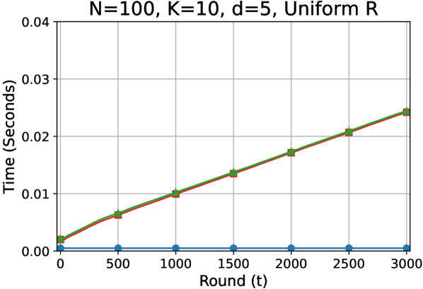
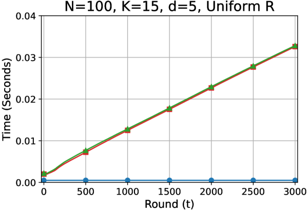
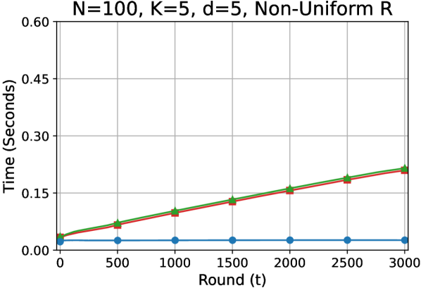
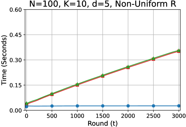
Figure I.1: Runtime per round under uniform rewards (first row) and non-uniform rewards (second row).

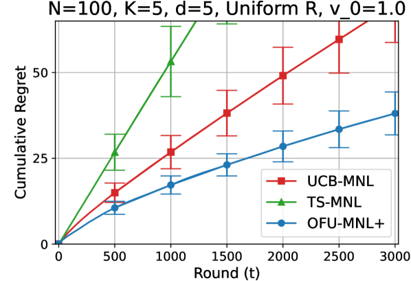
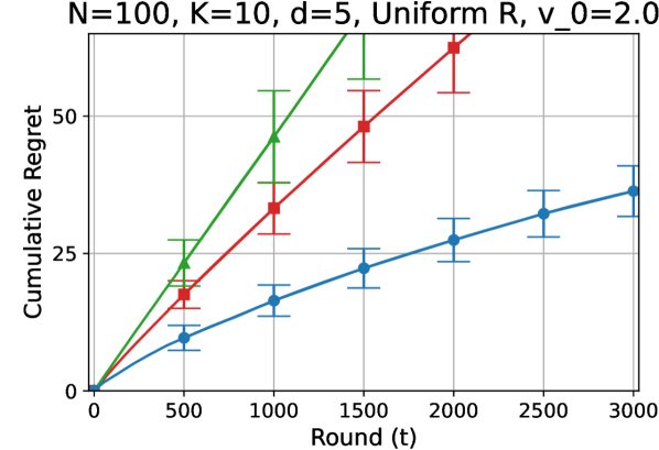
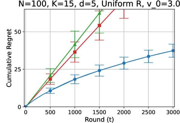
Figure I.2: Cumulative regret under uniform rewards with $v_{0}=\Theta(K)$.

References

- Abbasi-Yadkori et al. [2011] Yasin Abbasi-Yadkori, Dávid Pál, and Csaba Szepesvári. Improved algorithms for linear stochastic bandits. Advances in neural information processing systems, 24:2312–2320, 2011.
- Abeille and Lazaric [2017] Marc Abeille and Alessandro Lazaric. Linear Thompson Sampling Revisited. In Aarti Singh and Jerry Zhu, editors, Proceedings of the 20th International Conference on Artificial Intelligence and Statistics, volume 54 of Proceedings of Machine Learning Research, pages 176–184. PMLR, 20–22 Apr 2017.
- Abeille et al. [2021] Marc Abeille, Louis Faury, and Clément Calauzènes. Instance-wise minimax-optimal algorithms for logistic bandits. In International Conference on Artificial Intelligence and Statistics, pages 3691–3699. PMLR, 2021.
- Agrawal et al. [2023] Priyank Agrawal, Theja Tulabandhula, and Vashist Avadhanula. A tractable online learning algorithm for the multinomial logit contextual bandit. European Journal of Operational Research, 310(2):737–750, 2023.
- Agrawal and Goyal [2013] Shipra Agrawal and Navin Goyal. Thompson sampling for contextual bandits with linear payoffs. In International Conference on Machine Learning, pages 127–135. PMLR, 2013.
- Agrawal et al. [2017] Shipra Agrawal, Vashist Avadhanula, Vineet Goyal, and Assaf Zeevi. Thompson sampling for the mnl-bandit. In Conference on learning theory, pages 76–78. PMLR, 2017.
- Agrawal et al. [2019] Shipra Agrawal, Vashist Avadhanula, Vineet Goyal, and Assaf Zeevi. Mnl-bandit: A dynamic learning approach to assortment selection. Operations Research, 67(5):1453–1485, 2019.
- Amani and Thrampoulidis [2021] Sanae Amani and Christos Thrampoulidis. Ucb-based algorithms for multinomial logistic regression bandits. Advances in Neural Information Processing Systems, 34:2913–2924, 2021.
- Auer et al. [2002] Peter Auer, Nicolo Cesa-Bianchi, and Paul Fischer. Finite-time analysis of the multiarmed bandit problem. Machine learning, 47(2):235–256, 2002.
- Campolongo and Orabona [2020] Nicolo Campolongo and Francesco Orabona. Temporal variability in implicit online learning. Advances in neural information processing systems, 33:12377–12387, 2020.
- Chen et al. [2013] Wei Chen, Yajun Wang, and Yang Yuan. Combinatorial multi-armed bandit: General framework and applications. In International conference on machine learning, pages 151–159. PMLR, 2013.
- Chen and Wang [2018] Xi Chen and Yining Wang. A note on a tight lower bound for capacitated mnl-bandit assortment selection models. Operations Research Letters, 46(5):534–537, 2018.
- Chen et al. [2020] Xi Chen, Yining Wang, and Yuan Zhou. Dynamic assortment optimization with changing contextual information. The Journal of Machine Learning Research, 21(1):8918–8961, 2020.
- Chen et al. [2021] Xi Chen, Yining Wang, and Yuan Zhou. Optimal policy for dynamic assortment planning under multinomial logit models. Mathematics of Operations Research, 46(4):1639–1657, 2021.
- Cheung and Simchi-Levi [2017] Wang Chi Cheung and David Simchi-Levi. Thompson sampling for online personalized assortment optimization problems with multinomial logit choice models. Available at SSRN 3075658, 2017.
- Chu et al. [2011] Wei Chu, Lihong Li, Lev Reyzin, and Robert Schapire. Contextual bandits with linear payoff functions. In Proceedings of the Fourteenth International Conference on Artificial Intelligence and Statistics, pages 208–214. JMLR Workshop and Conference Proceedings, 2011.
- Davis et al. [2014] James M Davis, Guillermo Gallego, and Huseyin Topaloglu. Assortment optimization under variants of the nested logit model. Operations Research, 62(2):250–273, 2014.
- Faury et al. [2020] Louis Faury, Marc Abeille, Clément Calauzènes, and Olivier Fercoq. Improved optimistic algorithms for logistic bandits. In International Conference on Machine Learning, pages 3052–3060. PMLR, 2020.
- Faury et al. [2022] Louis Faury, Marc Abeille, Kwang-Sung Jun, and Clément Calauzènes. Jointly efficient and optimal algorithms for logistic bandits. In International Conference on Artificial Intelligence and Statistics, pages 546–580. PMLR, 2022.
- Filippi et al. [2010] Sarah Filippi, Olivier Cappé, Aurélien Garivier, and Csaba Szepesvári. Parametric bandits: The generalized linear case. In Proceedings of the 23rd International Conference on Neural Information Processing Systems - Volume 1, NIPS’10, page 586–594, Red Hook, NY, USA, 2010. Curran Associates Inc.
- Foster et al. [2018] Dylan J Foster, Satyen Kale, Haipeng Luo, Mehryar Mohri, and Karthik Sridharan. Logistic regression: The importance of being improper. In Conference on learning theory, pages 167–208. PMLR, 2018.
- Hazan et al. [2016] Elad Hazan et al. Introduction to online convex optimization. Foundations and Trends® in Optimization, 2(3-4):157–325, 2016.
- Jun et al. [2017] Kwang-Sung Jun, Aniruddha Bhargava, Robert Nowak, and Rebecca Willett. Scalable generalized linear bandits: Online computation and hashing. Advances in Neural Information Processing Systems, 30, 2017.
- Kazerouni and Wein [2021] Abbas Kazerouni and Lawrence M Wein. Best arm identification in generalized linear bandits. Operations Research Letters, 49(3):365–371, 2021.
- Kim et al. [2023] Wonyoung Kim, Kyungbok Lee, and Myunghee Cho Paik. Double doubly robust thompson sampling for generalized linear contextual bandits. In Proceedings of the AAAI Conference on Artificial Intelligence, volume 37, pages 8300–8307, 2023.
- Kveton et al. [2015] Branislav Kveton, Zheng Wen, Azin Ashkan, and Csaba Szepesvari. Tight regret bounds for stochastic combinatorial semi-bandits. In Artificial Intelligence and Statistics, pages 535–543. PMLR, 2015.
- Kveton et al. [2020] Branislav Kveton, Manzil Zaheer, Csaba Szepesvari, Lihong Li, Mohammad Ghavamzadeh, and Craig Boutilier. Randomized exploration in generalized linear bandits. In International Conference on Artificial Intelligence and Statistics, pages 2066–2076. PMLR, 2020.
- Lattimore and Szepesvári [2020] Tor Lattimore and Csaba Szepesvári. Bandit algorithms. Cambridge University Press, 2020.
- Lee et al. [2024] Junghyun Lee, Se-Young Yun, and Kwang-Sung Jun. Improved regret bounds of (multinomial) logistic bandits via regret-to-confidence-set conversion. In International Conference on Artificial Intelligence and Statistics, pages 4474–4482. PMLR, 2024.
- Li et al. [2017] Lihong Li, Yu Lu, and Dengyong Zhou. Provably optimal algorithms for generalized linear contextual bandits. In International Conference on Machine Learning, pages 2071–2080. PMLR, 2017.
- Liu et al. [2023] Xutong Liu, Jinhang Zuo, Siwei Wang, John CS Lui, Mohammad Hajiesmaili, Adam Wierman, and Wei Chen. Contextual combinatorial bandits with probabilistically triggered arms. In International Conference on Machine Learning, pages 22559–22593. PMLR, 2023.
- McFadden [1977] Daniel McFadden. Modelling the choice of residential location. 1977.
- Mhammedi et al. [2019] Zakaria Mhammedi, Wouter M Koolen, and Tim Van Erven. Lipschitz adaptivity with multiple learning rates in online learning. In Conference on Learning Theory, pages 2490–2511. PMLR, 2019.
- Miao and Chao [2021] Sentao Miao and Xiuli Chao. Dynamic joint assortment and pricing optimization with demand learning. Manufacturing & Service Operations Management, 23(2):525–545, 2021.
- Oh and Iyengar [2019] Min-hwan Oh and Garud Iyengar. Thompson sampling for multinomial logit contextual bandits. Advances in Neural Information Processing Systems, 32, 2019.
- Oh and Iyengar [2021] Min-hwan Oh and Garud Iyengar. Multinomial logit contextual bandits: Provable optimality and practicality. In Proceedings of the AAAI Conference on Artificial Intelligence, volume 35, pages 9205–9213, 2021.
- Orabona [2019] Francesco Orabona. A modern introduction to online learning. arXiv preprint arXiv:1912.13213, 2019.
- Ou et al. [2018] Mingdong Ou, Nan Li, Shenghuo Zhu, and Rong Jin. Multinomial logit bandit with linear utility functions. In Proceedings of the Twenty-Seventh International Joint Conference on Artificial Intelligence, IJCAI-18, pages 2602–2608. International Joint Conferences on Artificial Intelligence Organization, 2018.
- Perivier and Goyal [2022] Noemie Perivier and Vineet Goyal. Dynamic pricing and assortment under a contextual mnl demand. Advances in Neural Information Processing Systems, 35:3461–3474, 2022.
- Qin et al. [2014] Lijing Qin, Shouyuan Chen, and Xiaoyan Zhu. Contextual combinatorial bandit and its application on diversified online recommendation. In Proceedings of the 2014 SIAM International Conference on Data Mining, pages 461–469. SIAM, 2014.
- Rejwan and Mansour [2020] Idan Rejwan and Yishay Mansour. Top- combinatorial bandits with full-bandit feedback. In Aryeh Kontorovich and Gergely Neu, editors, Proceedings of the 31st International Conference on Algorithmic Learning Theory, volume 117 of Proceedings of Machine Learning Research, pages 752–776. PMLR, 08 Feb–11 Feb 2020.
- Rusmevichientong et al. [2010] Paat Rusmevichientong, Zuo-Jun Max Shen, and David B Shmoys. Dynamic assortment optimization with a multinomial logit choice model and capacity constraint. Operations research, 58(6):1666–1680, 2010.
- Sauré and Zeevi [2013] Denis Sauré and Assaf Zeevi. Optimal dynamic assortment planning with demand learning. Manufacturing & Service Operations Management, 15(3):387–404, 2013.
- Tran-Dinh et al. [2015] Quoc Tran-Dinh, Yen-Huan Li, and Volkan Cevher. Composite convex minimization involving self-concordant-like cost functions. In Modelling, Computation and Optimization in Information Systems and Management Sciences: Proceedings of the 3rd International Conference on Modelling, Computation and Optimization in Information Systems and Management Sciences-MCO 2015-Part I, pages 155–168. Springer, 2015.
- Zhang et al. [2016] Lijun Zhang, Tianbao Yang, Rong Jin, Yichi Xiao, and Zhi-Hua Zhou. Online stochastic linear optimization under one-bit feedback. In International Conference on Machine Learning, pages 392–401. PMLR, 2016.
- Zhang and Luo [2024] Mengxiao Zhang and Haipeng Luo. Contextual multinomial logit bandits with general value functions. arXiv preprint arXiv:2402.08126, 2024.
- Zhang and Sugiyama [2024] Yu-Jie Zhang and Masashi Sugiyama. Online (multinomial) logistic bandit: Improved regret and constant computation cost. Advances in Neural Information Processing Systems, 36, 2024.
- Zong et al. [2016] Shi Zong, Hao Ni, Kenny Sung, Nan Rosemary Ke, Zheng Wen, and Branislav Kveton. Cascading bandits for large-scale recommendation problems. In Proceedings of the Thirty-Second Conference on Uncertainty in Artificial Intelligence, page 835–844. AUAI Press, 2016.