Phase Retrieval from the Hong-Ou-Mandel Dip to Characterize the Phase Spectrum of Independent Pulses at the Single-Photon Level
Abstract
Measuring the phase spectrum at the single-photon level is essential for the full characterization of the temporal-spectral mode of quantum sources. We present a phase retrieval algorithm-based method to recover the phase spectrum difference between two independent pulses from their Hong-Ou-Mandel interference pattern and intensity spectra. Our confirmatory experiment with coherent state pulses confirms the accuracy of the recovered phase spectrum difference to within ±0.1 rad. The method we employ is readily generalizable to the measurement of single-photon wave packets and even correlated photon pairs.
1 Introduction
The characterization of the temporal-spectral mode of quantum sources plays an important role in the research of quantum information protocols using the temporal mode for encoding [1, 2]. While the majority of protocols necessitate only a technique for distinguishing orthogonal modes, the full characterization of the temporal-spectral mode still helps the field of study [3, 4, 5] . At the single-photon level, the measurement of the optical intensity spectrum can be achieved by replacing the detectors utilized in classical schemes with single-photon detectors[6, 7]. However, the nonlinear-based techniques for the temporal-spectral mode characterization, such as Frequency-Resolved Optical Gating (FROG)[8], can not be extended to the single-photon regime directly as the nonlinear effects are weak[9]. The characterization of the phase spectrum, or the full characterization of the temporal-spectral mode is an ongoing research area with new methods continually emerging [10, 11, 9, 12, 13, 14, 15].
The Hong-Ou-Mandel (HOM) interference can be used to analyze temporal-spectral properties of incident fields. HOM interference is the bunching effect when identical fields incident a beam splitter (BS) from different directions and is depicted by the reduction of coincidence rate[16]. The change of coincidence rate with respect to relative delay between incident photons is called the HOM interference pattern or HOM dip. The visibility of interference pattern is affected by the photon statistic feature and indistinguishability between incident photons[17], including their polarization, frequency, intensity, etc. For HOM interference between two independent pulses, the shape of the interference pattern is determined by the mode matching degree[18], which is quantified by the square magnitude of the cross-correlation function between their temporal-spectral mode. While many studies have investigated how the temporal-spectral mode affects the interference pattern, especially when dispersion is introduced into incident fields across various quantum states, such as the thermal state, single-photon state, and coherent state[19, 20, 21], fewer addressed the extraction of mode information from the pattern, such as linear chirp[22] and pulse width of the incident fields[21, 23]. This disparity signifies a considerable research opportunity.
To enrich the temporal-spectral information gleaned from the HOM interference pattern, we present a phase retrieval algorithm-based method to recover the phase spectrum difference (PSD) between independent incident fields from their HOM interference pattern and intensity spectra. Our theoretical and experimental frameworks are constructed around a specific unbalanced Mach-Zehnder interferometer setup[23, 18], where HOM interference between coherent pulses happens. In this condition, the PSD is entirely introduced by the dispersion medium on the interferometer arms, which is realized by a programmable filter (PF) in the experiment. By comparing the reconstructed PSD with the phase function input to the PF, we can gauge the accuracy of our method. Furthermore, our method is easy to generalize to the characterization of the phase spectrum of a single-photon wave packet, and even to the joint spectrum phase (JSP) of frequency-correlated photon pairs, a field that has seen few relevant studies in recent years[24, 25, 26, 27].
2 Theory
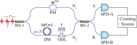
The schematic of the UBMZI is shown in Fig. 1, where represent pulses incidenting the BS-2 from different directions, as the optical path is not equivalent in a UBMZI, pulses meeting at the BS-2 are not from the same pulse of the source. The field function at is:
| (1) |
| (2) |
where represents the magnitude of pulses. is the normalized function of temporal mode. All the are random variables, where is the global phase of the pulses and is the phase introduced by a phase modulator (PM). are not independent of each other but independent of . The PM is used to introduce a random phase for each incident pulse, leading . In the Heisenberg picture, the equation of field operators on each side of a BS can be written as:
| (3) |
In the scenario where the reaction time of the SPD is much slower than the pulse duration, according to Glauber’s theory[28], the probabilities of detecting a photon in channel A, in channel B, and in both channels simultaneously can be respectively expressed as follows:
| (4) |
| (5) | ||||
| (6) |
where is the coefficient of the detector. For coherent states, the probability remains dependent on the global phase of each pulse. To accurately represent the real-world measurements, we still need to employ the ensemble average. So the normalized coincidence rate of delay is:
| (7) |
where , the mode matching degree is the square modulus of the cross-correlation function between the temporal mode function defined by:
| (8) |
Eq.(5) depicts the interference pattern and it is similar to the HOM interference between independent single-photon wave packet, where . Based on this similarity, many researches investigating the HOM interference of phase-independent sources used Mach-Zehnder Interferometer [26, 29, 30] or Michelson Interferometer [22, 31] with a PM introducing random phase and coherent pulsed source instead of a single photon source to simplify the experiment process.
As the source is a periodic pulse train in coherent state with temporal mode function , the temporal mode on the two interference arms is:
| (9) |
| (10) |
where is the PSD introduced by the dispersion medium. According to the generalized Wiener-Khintchine theorem, can be expressed as integration in the frequency domain:
| (11) |
where is the normalized spectrum of the incident beam which can be characterized by measuring the intensity spectrum, and is the PSD introduced by the dispersion medium. From Eq. (9), is the square modulus of Fourier transform of , while is the square modulus of it, similar to the relationship among the intensity functions on the Fraunhofer diffraction plane, the imaging plane, and the complex wave function, in a classical one-dimensional phase retrieval problem[32].
To reconstruct the PSD from intensity spectrum and mode matching degree, we adapted the Gerchberg-Saxton (G-S) algorithm, which has a mathmatical proof of convergence and has been realized and examined in other research domains before, for example, image recovery [33] and FROG [34].
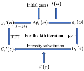
The G-S algorithm can be logically depicted in Fig. 2. is the current guess of , and is the current guess of the V. This iteration procedure only requires doing a Fourier transformation on the guess functions between two domains, concurrently substituting their magnitude with and . Equations at the th iteration can be expressed as:
| (12) |
where is generated from . According to the binomial distribution feature of the measured counting rate, the signal-to-noise ratio is low at the edge of the interference pattern. Therefore, in the final iterations, the second line of Eq. (10) should be modified to:
| (13) |
where is smaller than a certain value to mitigate the contribution of data points with a low signal-to-noise ratio to the overall result.
3 experiment
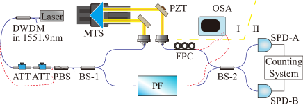
Fig. 3. illustrates our experimental setup, where a mode-locked fiber laser generates coherent pulses. These pulses are filtered by a Dense Wavelength Division Multiplexer (DWDM) to produce a 1.2 nm-wide spectrum. Passing through two ATTs, the pulses’ intensity is attenuated for photon-counting detection, ensuring a direct proportionality between the counting rate and intensity. A Polarization Beam Splitter (PBS) then polarizes the pulses. On the signal arm, a Finisar 4000A WaveShaper is functioning as the programmable filter (PF) to impose an arbitrary phase function , which corresponds to the PSD. On the reference arm, an electronic translation stage with a right-angle prism serves as the ODL. This setup allows for precise and programmable control over the relative delay. Additionally, a Piezoelectric Transducer (PZT) is positioned as a PM. The PZT is driven by a periodic triangular voltage signal, resulting in a phase modulation with an amplitude corresponding to a phase shift, to ensure that over a long period of counting time so that the pulses meeting at BS-2 are effectively phase-independent.
The optical path difference between the two arms is m, corresponding to twice the pulse interval of the optic source. This design allows the length difference of the single-mode fiber in the two arms to be minimized to m, reducing the impact of dispersion on the interference pattern to a level much smaller than that of the counting noise. With an incident pulse spectrum of 1.2 nm width, the width of is about 20 to 35 ps. In this research, the step size of the motorized translation stage is either 0.1 mm or 0.15 mm, corresponding to 2/3 ps or 1 ps, respectively. Consequently, the system would not be sensitive to optical path length instability.
The measurement is divided into two steps: In Step I, with the ATTs not engaged in the optical path, the spectrum of the pulses on both arms is measured. This step is crucial because the WaveShaper introduces a significant insertion loss spectrum, particularly when the slope of is steep, resulting in a difference in the spectra on the two arms. An equivalent spectrum for use in experiments is characterized by the expression , which is the square modulus of the cross-spectrum intensity. In Step II, pairs of pulses at the single-photon level incident on BS-2, which is connected to two SPDs, where counting rates will be recorded at different relative delay and a normalized coincidence rate will be calculated to derive the mode matching degree .
The ways to raise the accuracy of measured patterns are enhancing the counting rate and sampling duration. If the counting rate is too high, the nonlinear relationship between the counting rate and intensity will be obvious, resulting in a reduced expected value for the single-channel counting rate and an increased expected value for the normalized coincidence rate. In order to ensure the accuracy and efficiency of the measurement, in our experiment, the counting rate of SPD is about M/s, while the repetition rate of the optic source is about 36.88 MHz, and dead time is about ns on average. It takes to measure the coincidence rate at each sampling point for the first experiment and 90 s for the second one.
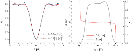
Fig. 4 shows the HOM dip and recovered phase function when . From Fig. 4(b),it can be observed that the reconstructed phase function is a smooth curve near zero for frequencies with strong intensity. As the intensity spectrum drops for higher or lower frequency components, the phase function increasingly resembles a random value. This randomness is due to the minimal contribution of the weaker intensity frequency components to the interference pattern, leading to less accurate reconstruction of the phase at corresponding frequency.
Unmatched polarization and intensity differences between the incident photons will reduce the contrast ratio of the interference pattern alerting the shape, which means that the overall amplitude of the measured function . However, as our algorithm is an iterative Fourier transform method, the overall amplitude wouldn’t affect the . Reversely, The iteration outcomes can be used to correct the measured interference pattern. We plot the corrected interference pattern in Fig. 4, where is equal to 1.1027 in this experiment. The lowest point of the recovered HOM dip is 0.505, which is close to 0.5, indicating that the dispersion effects due to the length difference in fibers and other elements are negligible. Furthermore, we manually aligned the lowest point of the HOM dip with . This manual calibration serves as a reference for the relative delay, assisting in the detrending of the recovered phase function. This deliberate calibration helps to reduce the need for further manual manipulation when making comparisons, allowing for a more scientific and less subjective comparison between and .
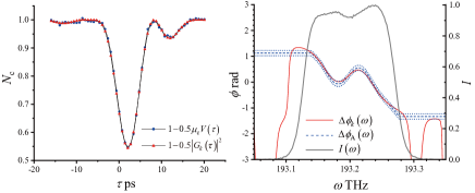
Fig. 5 shows the HOM dip and recovered phase function when introducing an "inverted N-shaped" function . Prior to the experiment, we simulated the effects of counting noise by incorporating the binomial distribution characteristic of single-channel counting. Our simulations revealed that the majority of the recovered fall within the interval rad between 193.13 193.25 THz. As the recovered function in Fig. 5.(b) is in this confidence interval, the noise from the counting distribution dominates the error, proving that our method can successfully recover the PSD between the two incident pulses.
In both simulation and experiment, we found that the specific phase retrieval problem we processed presents a double solution problem: the reconstructed may converge to , which is centrally symmetric to , this phenomenon is particularly evident when the spectrum is symmetric or the noise is high. However, the mode matching degree corresponding to the incorrect convergence results will show a greater difference compared to the correct convergence results when compared to the actual mode matching degree . Therefore, we run the algorithm with varied initial values and compare the results to address the double solution issue.
The scenario in our last experiment can be likened to measuring the phase spectrum of an unknown pulse from its intensity spectrum and HOM dip with a known reference pulse in a coherent state. Notably, the presence of an insertion loss spectrum in the PF, which already caused a distinct dip in the spectrum in Fig. 5.(b), doesn’t hinder our method, proving that our method works even when the two incident fields have differing intensity spectra. Ideally, reference pulse spectrum should be marginally wider than unknown pulse spectrum to fully reconstruct phase spectrum.
4 Summary
In this paper, we present a method for reconstructing the PSD between two phase-independent pulses in a coherent state from their HOM interference patterns and intensity spectra, employing an adapted Gerchberg-Saxton (G-S) algorithm. To evaluate the effectiveness of our method, we performed experiments using a UBMZI. The experiment outcomes indicate that the reconstructed PSD approximated the actual PSD introduced by the PF, with a discrepancy of ±0.1 radians.
Through our method, the phase spectrum of a single-photon wave packet can be characterized by measuring the interference pattern with a well-defined wave packet in a coherent state. This approach can be extended to fully characterize the Joint Spectrum Amplitude (JSA) of frequency-correlated photon pairs, with two proposed methods for measurement. The first method involves combining our approach with heralded single-photon source technology, akin to the technique referenced in [35]. The second method entails reconstructing the JSA from both the Joint Spectrum Intensity (JSI) and Joint Temporal Intensity (JTI). They are all measurable experimentally now, as demonstrated in [6, 36, 7] and [37, 38], and happen to be intensity function of JSA on the original domain and the Fourier trans form domain, presenting a classic two-dimensional phase retrieval problem.
Our study affirms the practical application relationship between HOM interference and the nonlinear harmonic generation process. The Chripled Pulsed Interferometer is seen as the time-reversal version of the HOM interference [39], where the HOM dip-like interference pattern comes from a Sum-frequency generation. Conversely, pulse width measurement via HOM interference relies on the correlation function within the interference pattern[22], akin to the autocorrelation technique that utilizes second-order harmonic generation[40]. Advancing from autocorrelators, FROG enabled the full characterization of ultra-short pulse with the phase retrieval algorithm[8], with which we successfully reconstructed the PSD from the HOM interference pattern.
Acknowledgments We would like to acknowledge Professor Z.Y. Jeff Ou for constructive discussions.
References
- [1] A. I. Lvovsky and M. G. Raymer, \JournalTitleReviews of modern physics 81, 299 (2009).
- [2] J. L. O’brien, A. Furusawa, and J. Vučković, \JournalTitleNature photonics 3, 687 (2009).
- [3] W. Tittel and G. Weihs, \JournalTitleQuantum Inf. Comput. 1, 3 (2001).
- [4] C. H. Bennett, P. W. Shor, J. A. Smolin, and A. V. Thapliyal, \JournalTitlePhysical Review Letters 83, 3081 (1999).
- [5] M. G. Raymer, A. H. Marcus, J. R. Widom, and D. L. P. Vitullo, \JournalTitleThe journal of physical chemistry. B 117 49, 15559 (2013).
- [6] B. J. Smith, P. Mahou, O. Cohen, et al., \JournalTitleOptics express 17 26, 23589 (2009).
- [7] A. O. Davis, P. M. Saulnier, M. Karpiński, and B. J. Smith, \JournalTitleOptics Express 25, 12804 (2017).
- [8] R. Trebino and D. J. Kane, \JournalTitleJournal of The Optical Society of America A-optics Image Science and Vision 10, 1101 (1993).
- [9] A. O. C. Davis, V. Thiel, M. Karpiński, and B. J. Smith, \JournalTitlePhys. Rev. Lett. 121, 083602 (2018).
- [10] Z. Qin, A. S. Prasad, T. Brannan, et al., \JournalTitleLight: Science & Applications 4, e298 (2015).
- [11] C. Polycarpou, K. Cassemiro, G. Venturi, et al., \JournalTitlePhysical review letters 109, 053602 (2012).
- [12] V. Ansari, J. M. Donohue, M. Allgaier, et al., \JournalTitlePhysical review letters 120, 213601 (2018).
- [13] N. Huo, Y. Liu, J. Li, et al., \JournalTitlePhys. Rev. Lett. 124, 213603 (2020).
- [14] V. Thiel, A. O. C. Davis, K. Sun, et al., “Single-photon characterization by spectrally-resolved hong-ou-mandel interference,” in Rochester Conference on Coherence and Quantum Optics (CQO-11), (Optica Publishing Group, 2019), p. M5A.21.
- [15] W. Wasilewski, P. Kolenderski, and R. Frankowski, \JournalTitlePhysical review letters 99, 123601 (2007).
- [16] C. Hong, Z. Ou, and L. Mandel, \JournalTitlePhysical review letters 59, 2044—2046 (1987).
- [17] A. J. Menssen, A. E. Jones, B. J. Metcalf, et al., \JournalTitlePhysical Review Letters. 118, 153603 (2017).
- [18] Z. Y. Ou and X. Li, \JournalTitlePhys. Rev. Res. 4, 023125 (2022).
- [19] Xiaoxin, Ma, Liang, et al., \JournalTitleJournal of the Optical Society of America B 32, 946 (2015).
- [20] X. Ma, X. Li, L. Cui, et al., \JournalTitlePhysical Review A 84, 023829 (2011).
- [21] Y.-R. Fan, C.-Z. Yuan, R.-M. Zhang, et al., \JournalTitlePhotonics Research 9, 1134 (2021).
- [22] Y, Miyamoto, T, et al., \JournalTitleOptics Letters (1993).
- [23] W. Zhao, N. Huo, L. Cui, et al., \JournalTitleOpt. Express 30, 447 (2022).
- [24] I. Jizan, B. Bell, L. G. Helt, et al., \JournalTitleOptics Letters 41, 4803 (2016).
- [25] A. O. C. Davis, V. Thiel, and B. J. Smith, “Measuring the temporal-spectral state of two photons,” in Conference on Coherence and Quantum Optics, (2019).
- [26] G. S. Thekkadath, B. A. Bell, R. B. Patel, et al., \JournalTitlePhys. Rev. Lett. 128, 023601 (2022).
- [27] K. Zielnicki, K. Garay-Palmett, D. Cruz-Delgado, et al., \JournalTitleJournal of Modern Optics 65, 1141 (2018).
- [28] R. J. Glauber, \JournalTitlePhysical Review 130, 2529 (1963).
- [29] Y.-S. Kim, O. Slattery, P. S. Kuo, and X. Tang, \JournalTitlePhys. Rev. A 87, 063843 (2013).
- [30] Y.-R. Fan, C.-Z. Yuan, R.-M. Zhang, et al., \JournalTitlePhoton. Res. 9, 1134 (2021).
- [31] H. Kim, O. Kwon, and H. S. Moon, \JournalTitleScientific Reports 11, 20555 (2021).
- [32] J, R, and Fienup, \JournalTitleApplied Optics (1982).
- [33] R. W. Gerchberg, \JournalTitleOptik 35, 237 (1972).
- [34] J. Paye, M. Ramaswamy, J. G. Fujimoto, and E. P. Ippen, \JournalTitleOptics letters 18, 1946 (1993).
- [35] G. S. Thekkadath, B. A. Bell, R. B. Patel, et al., \JournalTitlePhys. Rev. Lett. 128, 023601 (2022).
- [36] B. Fang, O. Cohen, M. Liscidini, et al., \JournalTitleOptica 1, 281 (2014).
- [37] J.-P. W. Maclean, J. M. Donohue, and K. J. Resch, \JournalTitlePhysical review letters 120 5, 053601 (2017).
- [38] R.-B. Jin, T. Saito, and R. Shimizu, \JournalTitlePhysical Review Applied 10, 034011 (2018).
- [39] R. Kaltenbaek, J. Lavoie, D. N. Biggerstaff, and K. J. Resch, \JournalTitleNature Physics 4, 864 (2008).
- [40] H. Pike and M. Hercher, \JournalTitleJournal of Applied Physics 41, 4562 (1970).