Three-body forces and Efimov physics in nuclei and atoms

Abstract

This review article presents historical developments and recent advances in our understanding on the three-body forces and Efimov physics, from an interdisciplinary viewpoint encompassing nuclear physics and cold atoms. Theoretical attempts to elucidate the three-body force with the chiral effective field theory are explained, followed by an overview of experiments aimed at observing signatures of the nuclear three-body force. Some recent experimental and theoretical works in the field of cold atoms devoted to measuring and engineering three-body forces among atoms are also presented. As a phenomenon arising from the three-body effect, Efimov physics in both cold atoms and nuclear systems is reviewed.

1 Introduction

All visible matter in the universe is organized into resolution-dependent hierarchical structures. A precise description of the interactions at each hierarchical level starting from elementary quarks to composite systems like hadrons, nuclei, atoms and molecules may help to improve our understanding of the structure and dynamics of strongly interacting matter. Generally, effective interactions at all hierarchical levels are dominated by pairwise forces acting between two constituent particles. Meanwhile, recent advances in computational, theoretical and experimental techniques allow one to go beyond the two-body-force level and to quantitatively probe three-body interactions, which are known to figure importantly in atomic and nuclear systems Hammer:2012id .

Historically, the most well known three-body force model was proposed by Fujita and Miyazawa in 1957 10.1143/PTP.17.360 to describe nuclear systems using protons and neutrons, jointly called nucleons, as constituent particles. The Fujita-Miyazawa type three-nucleon force ($3N$F), visualized by the Feynmann diagram in Fig. 1, is driven by virtual pion-nucleon scattering with an intermediate excitation of the nucleon into the $\Delta(1232)$ resonance. Three-nucleon forces are thus intimately related to the inner structures of the nucleons and their short-distance virtual excitations.

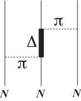
Figure 1: Feynmann diagram of Fujita-Miyazawa type three-nucleon force.

Following the idea of Fujita and Miyazawa, one may expect three-body forces to play an important role in quantum systems other than atomic nuclei. With their high controllability, cold atoms have recently emerged as an excellent platform to explore quantum systems of interests. It is possible to realize cold-atom systems where the three-body forces among atoms appear from similar exchanges of virtual excitations, thereby quantum-simulating the Fujita-Miyazawa mechanism. It is even possible to engineer the strength of the three-body force and thereby realize a system where the three-body force has significant effects on few- and many-body properties, in stark contrast to conventional systems where the two-body force dominates over the three-body force.

The emergence of a three-body force from exchange processes can lead to an even more exotic phenomenon, the Efimov effect. When three particles scatter with each other via resonant two-body interactions, a long-range three-body force emerges via multiple scatterings. The three-body force is attractive and forms a series of weakly bound three-body states, known as the Efimov states. The Efimov states have not only been observed in cold-atom experiments, but they appear universally in various physical systems. Thanks to its universal properties, Efimov physics provides a unified description of various classes of three-body phenomena in cold atoms and nuclear physics.

In this review article, we discuss three-body forces in nuclear systems and in cold atomic gases as a key aspect for bridging different hierarchies. We present an overview of the three-body force in nuclear systems in Sec. 2. After briefly presenting historical developments of the three-body forces in Sec. 2.1, we show in Sec. 2.2 the effective field theory (EFT) description of the three-body force in nuclei, followed by a review of the experimental studies in Sec. 2.3. In Sec. 3, we present recent studies in the field of cold atoms to realize and simulate the three-body forces. In Sec. 4, we show the recent developments of Efimov physics in cold atoms and nuclear systems.

2 Three-body forces in nuclei

2.1 Three-nucleon force and its importance in nuclear phenomena

Since Yukawa’s meson theory proposed in 1935 Yukawa193548 , the nuclear force has been modeled in terms of meson exchange interactions between nucleons. Beside the dominant two-nucleon forces, the three nucleon forces ($3N$Fs) have attracted an increasing attention in the last two decades. The development of high-precision two-nucleon potentials in the 90s of the last century, coupled with advances in ab initio few-body calculations based on these interactions, have confirmed the important role played by $3N$Fs in various nuclear phenomena. Following the seminal work by Fujita and Miyazawa, a number of the $3N$F models utilizing the longest-range $2\pi$-exchange mechanism have been developed such as, e.g., the Tucson-Melbourne 99 tm99 , the Urbana IX PhysRevC.56.1720 $3N$F models. A new impetus to study $3N$Fs has come from chiral perturbation theory, the low-energy effective field theory of QCD Weinberg:1990rz ; kolk1994 ; Epelbaum:2002vt .

Historically, the first indication for a missing $3N$F came from the three-nucleon bound states ${}^{3}\rm H$ and ${}^{3}\rm He$ PhysRevC.33.1740 ; FewBodySys.1.3 . The binding energies of these nuclei were found to be not reproduced by an exact solution of the three-nucleon Faddeev equation using high-precision phenomenological $NN$ forces including the Argonne $V_{18}$ (AV18) AV18 , CD Bonn cdb as well as Nijmegen I and II nijm potentials. The underbinding of ³H and ³He could be explained by adding a $2\pi$-exchange-type $3N$F PhysRevC.33.1740 ; FewBodySys.1.3 ; PhysRevC.65.054003 . The importance of $3N$Fs has also been noted in other instances. In particular, microscopic calculations of light and medium-mass nuclei carried out using ab initio methods such as, e.g., quantum Monte Carlo PhysRevC.66.044310 ; Piarulli:2017dwd , no-core shell model PhysRevC.68.034305 , coupled cluster theory Hagen:2012sh , self-consistent Green’s function method Cipollone:2014hfa and nuclear lattice simulations Lahde:2019npb highlight the important role of $3N$Fs in explaining the corresponding binding energies. Furthermore, short-range repulsive $3N$Fs are considered key elements in describing the nuclear equation of state and two-solar-mass neutron star properties PhysRevC.58.1804 ; Gandolfi:2013baa ; PhysRevLett.116.062501 . In the past two decades, low-energy nucleon-deuteron scattering, binding energies of light and medium-mass nuclei as well as the equation of state of nuclear matter have also been extensively studied in the framework of the chiral effective field theory epelbaum2009 ; Kalantar-Nayestanaki_2012 ; Hammer:2012id ; PhysRep21Hebeler . In all these investigations, it became evident that $3N$Fs are key elements to understand various nuclear phenomena.

Discussions of three-body forces in nuclei currently extend to strange baryonic systems, e.g. $NN\Lambda$ interactions, especially for the neutron star properties Haidenbauer:2016vfq , which are needed to establish a universal understanding of the forces acting in nuclear phenomena. Also, it is notable that discussions of $3N$Fs stimulate the investigation of three-body forces in different hierarchies. As described in Sec. 3, study of three-body forces in the cold-atom systems are in progress not only from the theoretical but also from the experimental point of view.

2.2 Three-nucleon forces in chiral effective field theory

2.2.1 Chiral perturbation theory

The interactions and dynamics of pions can be described using the most general effective Lagrangian $\mathcal{L}_{\pi}$ that features the approximate chiral symmetry of QCD. It includes all possible terms allowed by symmetry, multiplied with coefficients that are commonly referred to as low-energy constants (LECs). These LECs are not fixed by symmetry and carry information about short-range QCD dynamics. It is convenient to classify terms in the effective Lagrangian according to the number of derivatives and/or insertions of the pion mass $M_{\pi}$: $\mathcal{L}_{\pi}=\mathcal{L}_{\pi}^{(2)}+\mathcal{L}_{\pi}^{(4)}+\ldots$. Multi-pion scattering amplitudes for the physically intersting case of $p\sim M_{\pi}\neq 0$ can be calculated from the effective Lagrangian using chiral perturbation theory (ChPT) Weinberg:1978kz ; Gasser:1983yg , i.e. via a perturbative expansion in $Q\in\{p/\Lambda_{b},\,M_{\pi}/\Lambda_{b}\}$, where $\Lambda_{b}$ is the breakdown scale of ChPT, which may be estimated by the masses of lowest-lying resonances in the $\pi\pi$ system.

The perturbative approach outlined above can be straightforwardly generalized to processes involving a single non-Goldstone-boson particle such as, e.g., the nucleon. The most general pion-nucleon effective Lagrangian $\mathcal{L}_{\pi N}=\mathcal{L}_{\pi N}^{(1)}+\mathcal{L}_{\pi N}^{(2)}+\mathcal{L}_{\pi N}^{(3)}+\ldots$ can be constructed using the methods described in Refs. Weinberg:1968de ; Coleman:1969sm ; Callan:1969sn . The explicit form of $\mathcal{L}_{\pi N}^{(1)}$ and $\mathcal{L}_{\pi N}^{(2)}$ can be found, e.g., in Ref. Bernard:1995dp , while the Lagrangians $\mathcal{L}_{\pi N}^{(3)}$ and $\mathcal{L}_{\pi N}^{(4)}$ are given in Refs. Fettes:1998ud and Fettes:2000gb , respectively. Compared to the Goldstone-boson sector, special care is required for processes involving a nucleon to ensure that the hard scale set by the nucleon mass $m_{N}$ does not spoil the chiral power counting when computing loop diagrams. The simplest way to achieve this is to perform a non-relativistic expansion of the effective Lagrangian $\mathcal{L}_{\pi N}$ Jenkins:1990jv ; Bernard:1992qa . This ensures that $m_{N}$ appears in $\mathcal{L}_{\pi N}$ only in the form of $1/m_{N}^{n}$-corrections with $n>0$, and the corresponding framework is referred to as the heavy-baryon ChPT. It is also possible to perform calculations in a manifestly Lorentz-invariant way by choosing the appropriate renormalization conditions Becher:1999he ; Gegelia:1999gf ; Fuchs:2003qc .

2.2.2 Chiral EFT for nuclear systems

Clearly, a direct application of ChPT to systems involving two and more nucleons is not possible due to the non-perturbative nature of the nuclear interactions, as reflected in the existence of shallow bound states such as ²H, ³H, ³He, ⁴He, etc. These bound states manifest themselves as subthreshold poles of the corresponding scattering amplitudes and signal the breakdown of the perturbative expansion.

In the early 1990s, Weinberg came up with an approach that is based on the effective Lagrangian and allows one to analyze low-energy few- and many-nucleon systems in a model-independent and systematic fashion Weinberg:1990rz ; Weinberg:1991um , which is nowadays commonly referred to as chiral effective field theory (ChEFT). He has attributed the failure of perturbation theory in the few-nucleon sector to the appearance of enhanced few-nucleon-reducible ladder-type diagrams and argued that they need to be resummed non-perturbatively. He also noticed that a resummation of ladder-type diagrams is performed automatically by solving the corresponding Lippmann-Schwinger-type integral equations for the scattering amplitude. Thus, Weinberg’s ChEFT approach to few-nucleon systems technically reduces to the conventional A-body problem,

$$\bigg{[}\bigg{(}\sum_{i=1}^{A}\frac{-\vec{\nabla}_{i}^{2}}{2m_{N}}+\mathcal{O}(m_{N}^{-3})\bigg{)}+V_{NN}+V_{3N}+\ldots\bigg{]}\big{|}\Psi\big{\rangle}=E\big{|}\Psi\big{\rangle},$$ (1)

but it opens the possibility to derive nuclear interactions $V_{NN}$, $V_{3N}$, $V_{4N}$, $\ldots$, via a systematically improvable ChPT expansion in harmony with the symmetries of QCD. Here, nuclear potentials are defined by means of all possible few-nucleon-irreducible contributions to the scattering amplitude, which are not affected by the above-mentioned enhancement and can be derived in the framework of ChPT using a variety of methods. Following Weinberg’s original work Weinberg:1990rz ; Weinberg:1991um , time-ordered perturbation theory was employed in Refs. Ordonez:1995rz ; Pastore:2008ui ; Pastore:2009is ; Pastore:2011ip ; Baroni:2015uza to derive nuclear forces and electroweak currents. Another approach, the so-called method of unitary transformation (MUT), makes use of a unitary transformation of the pion-nucleon Hamiltonian to decouple the purely nucleonic subspace of the Fock space from the rest. The MUT was applied to derive few-nucleon forces as well as electroweak and scalar nuclear currents in Refs. Epelbaum:1998ka ; Epelbaum:1999dj ; Epelbaum:2002gb ; Epelbaum:2005fd ; Epelbaum:2005bjv ; Epelbaum:2007us ; Bernard:2007sp ; Bernard:2011zr ; Krebs:2012yv ; Krebs:2013kha ; Kolling:2009iq ; Kolling:2011mt ; Krebs:2016rqz ; Krebs:2019aka ; Krebs:2020plh . Yet another method to derive the $NN$ two- and three-pion exchange potentials from matching to the scattering amplitude was applied in Refs. Kaiser:1997mw ; Kaiser:1998wa ; Kaiser:1999ff ; Kaiser:1999jg ; Kaiser:2001dm ; Kaiser:2001pc ; Kaiser:2001at ; Entem:2015xwa . For a detailed discussion of these techniques and applications the reader is referred to the review articles Epelbaum:2005pn ; epelbaum2009 ; Machleidt:2011zz ; Epelbaum:2019kcf ; Krebs:2020pii ; deVries:2020iea .

Non-perturbative resummations of reducible diagrams in ChEFT pose complications as compared with ChPT in the Goldstone-boson or single-nucleon sectors. Consider the longest-range $NN$ force due to the one-pion exchange

$$V_{NN}^{1\pi}(\vec{q}\,)=-\frac{g_{A}^{2}}{4F_{\pi}^{2}}\frac{\vec{\sigma}_{1}\cdot\vec{q}\vec{\sigma}_{2}\cdot\vec{q}}{q^{2}+M_{\pi}^{2}}\mbox{\boldmath$\tau$}_{1}\cdot\mbox{\boldmath$\tau$}_{2}\,,$$ (2)

where $g_{A}$ and $F_{\pi}$ are the nucleon axial vector coupling and the pion decay constant, respectively. Further, $\vec{\sigma}_{i}$ ($\mbox{\boldmath$\tau$}_{i}$) denote the spin (isospin) Pauli matrices of nucleon $i$, while $\vec{q}=\vec{p}\,^{\prime}-\vec{p}$, with $\vec{p}$ ($\vec{p}\,^{\prime}$) being the nucleon center-of-mass (CM) momentum in the initial (final) state, is the nucleon momentum transfer. The one-pion exchange potential (OPEP) contributes to the leading-order (i.e., order-$Q^{0}$) nuclear force and thus needs to be resummed non-perturbatively. However, the $1/r^{3}$ singularity in the tensor part of the OPEP implies the appearance of ultraviolet divergences in all spin-triplet channels upon performing iterations of the Lippmann-Schwinger (LS) equation. That is, removing ultraviolet divergences from the iterative solution of the LS equation requires the introduction of an infinite number of counter terms from the Lagrangians $\mathcal{L}_{NN}^{(0)}$, $\mathcal{L}_{NN}^{(2)}$, $\mathcal{L}_{NN}^{(4)}$, $\ldots$. This is in strong contrast to ChPT, where a finite number of counter terms are required to remove ultraviolet divergences at any given order.

Clearly, the singular short-distance nature of $V_{NN}^{1\pi}(\vec{q}\,)$ is unphysical and represents an artifact of using the low-momentum approximation in Eq. (2) beyond its validity range (i.e., at short distances or large values of the momentum transfer). Renormalization of the Schrödinger equation in EFTs with singular interactions like $V_{NN}^{1\pi}(\vec{q}\,)$ can be achieved in the way compatible with the weak-interaction limit by introducing a finite cutoff $\Lambda$ of the order of the pertinent hard scale, $\Lambda\sim\Lambda_{b}$ Lepage:1997cs . At each order of ChEFT and for every value of $\Lambda$, renormalization is carried out implicitly by expressing bare LECs from $\mathcal{L}_{NN}$, $\mathcal{L}_{NNN}$, $\ldots$, in terms of measurable quantities. In practice, this is achieved by tuning few-nucleon contact interactions to experimental data. The residual dependence of the renormalized results on the cutoff $\Lambda$ serves as a measure of the neglected contributions of terms beyond the EFT truncation level. It is expected to decrease with the chiral order and provides an a posteriori consistency check. In Refs. Gasparyan:2021edy ; Gasparyan:2023rtj , the finite-$\Lambda$ formulation of ChEFT was formally proven to be renormalizable (in the EFT sense) up to next-to-leading order $Q^{2}$ (NLO). Here and in what follows, we restrict ourselves to the finite-cutoff formulation of ChEFT as described in detail in Ref. Epelbaum:2019kcf . A pedagogical introduction into the considered framework can be found in Sec. 6.3 of Ref. Gross2022hyw , while a discretized (lattice) formulation is described in Ref. Lahde:2019npb .

2.2.3 Current status of the $NN$ potentials

Presently, the $NN$ force has been worked out completely up through fifth order $Q^{5}$ (i.e., N⁴LO) including isospin-breaking corrections due to $m_{u}\neq m_{d}$ and QED effects. It involves the one- two- and three-pion exchange potentials, supplemented by short-range NN interactions from $\mathcal{L}_{NN}^{(0)}$, $\mathcal{L}_{NN}^{(2)}$, and $\mathcal{L}_{NN}^{(4)}$, which depend on $2$, $7$ and $15$ LECs, respectively, that need to be tuned to $NN$ data. Notice that $3$ out of $15$ contact interactions at N⁴LO contribute only to the off-shell part of the $NN$ potential and thus cannot be determined from two-nucleon scattering data.

While semi-quantitative ChEFT potentials have a long history that goes back to the beginning of 2000s, see Refs. Epelbaum:2004fk ; Entem:2003ft for the first-generation order-$Q^{4}$ (i.e., N³LO) $NN$ potentials constructed using non-local regulators, the field has received new impetus in the last decade by developing a local regularization scheme for pion-exchange contributions that preserves the long-range behavior of the nuclear force, which allowed to significantly improve the predictive power of ChEFT Epelbaum:2014efa ; Epelbaum:2014sza . The state-of-the-art $NN$ N⁴LO⁺ potential of Ref. Reinert:2017usi employs a local momentum-space regulator for the OPEP and two-pion exchange potential (TPEP) via

$$V_{NN}^{1\pi}(\vec{q}\,) \to V_{NN}^{1\pi}(\vec{q}\,)\,e^{-\frac{q^{2}+M_{\pi}^{2}}{\Lambda^{2}}}+\ldots\,,$$ (3)

$$V_{NN}^{2\pi}(q\,) \to \frac{2}{\pi}\int_{2M_{\pi}}^{\infty}d\mu\mu\frac{\rho_{2\pi}(\mu)}{q^{2}+\mu^{2}}\,e^{-\frac{q^{2}+\mu^{2}}{2\Lambda^{2}}}+\ldots\,,$$ (4)

where the ellipses denote subtractions in the form of $NN$ contact interactions, chosen in such a way that the corresponding $r$-space potentials vanish at the origin. In the second equation, we have used a dispersive representation of the TPEP Kaiser:1997mw , where the spectral function $\rho_{2\pi}(\mu)$ is obtained from an analytic continuation of the unregularized potential $V_{NN}^{2\pi}(q)$ to imaginary values of $q$ via $\rho_{2\pi}(\mu):=\Im\big{[}V_{NN}^{2\pi}(0^{+}-i\mu)\big{]}$. Equations (3) and (4) show that all finite-$\Lambda$ artifacts stemming from the $1/\Lambda$-expansion of the regularized OPEP and TPEP have the form of short-range contact interactions. The latter are regularized in Ref. Reinert:2017usi using a Gaussian non-local regulator $\exp[-(p^{2}+p^{\prime 2})/\Lambda^{2}]$. The resulting semi-local momentum-space regularized (SMS) $NN$ potentials are available at orders LO through N⁴LO and cutoff values of $\Lambda=400$, $450$, $500$ and $550$ MeV. The N⁴LO⁺ potentials lead to a statistically perfect description of the Granada-2013 database of mutually consistent neutron-proton and proton-proton scattering data below pion production threshold NavarroPerez:2013usk and show, as expected, a very weak residual $\Lambda$-dependence. In Ref. Reinert:2020mcu , the SMS $NN$ potential of Ref. Reinert:2017usi was updated to include all relevant isospin-breaking contributions up through N⁴LO, and it was used for a precision determination of the $\pi N$ coupling constants from $NN$ scattering and to perform a full fledged partial wave analysis of $NN$ data (including a selection of mutually compatible data), see Ref. Epelbaum:2022cyo for details and Fig. 2 for representative examples

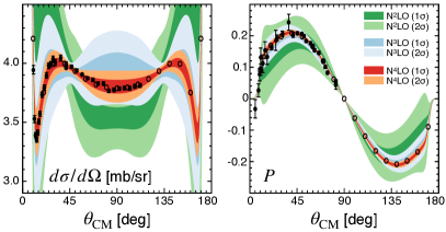
Figure 2: Proton-proton differential cross section at $E_{\rm lab}=144.1$ MeV (left panel) and the analyzing power $P$ at $E_{\rm lab}=142$ MeV (right panel) at N²LO (green bands), N³LO (blue bands) and N⁴LO⁺ (red bands) in ChEFT. Dark- and light-shaded bands show $1\sigma$ and $2\sigma$ confidence levels at the corresponding order, respectively, estimated using the Bayesian model $\bar{\rm C}^{650}_{0.5-10}$ from Ref. Epelbaum:2019zqc . Experimental data are shown by filled symbols and taken from Refs. Cox:1968jxz ; Jarvis:1971fla ; TAYLOR1960320 . Open circles are the results of the Nijmegen partial wave analysis Stoks:1993tb . See Ref. Epelbaum:2019kcf for more details.

These new developments allowed one to test the predictive power of ChEFT by quantitatively addressing the impact of the TPEP. In Refs. Epelbaum:2014efa ; Epelbaum:2014sza ; Reinert:2017usi , a clear evidence of the parameter-free contributions of the TPEP was observed at orders $Q^{3}$ (N²LO) and $Q^{5}$ (N⁴LO), where no additional $NN$ contact interactions appear. A significantly smaller number of adjustable parameters in the SMS potential of Refs. Epelbaum:2014sza ; Reinert:2017usi as compared to the phenomenological high-precision potential models provides yet another indication of the importance of the TPEP and demonstrates the predictive power of ChEFT. For related earlier studies along this line see Refs. Rentmeester:1999vw ; Birse:2003nz .

Other notable recent additions to the ChEFT $NN$ potentials involve the nonlocal N⁴LO⁺ potentials by the Idaho group Entem:2017gor as well as the (nearly) local N³LO potentials of Refs. Piarulli:2014bda ; Somasundaram2023sup ; Saha:2022oep .

2.2.4 Chiral expansion of the $3N$F

We now turn to the main subject of this article and review the applications of ChEFT to the $3N$F. It is instructive to first discuss the most general structure of a $3N$F. In the static limit of infinitely heavy nucleons, the potentials mediated by the exchange of one or multiple pions take a local form, i.e. they depend only on the momentum transfers $\vec{q}_{i}$ and not on the individual momenta $\vec{p}_{i}$, $\vec{p}_{i}^{\,\prime}$ of the nucleons. Assuming parity, time-reversal invariance and isospin symmetry, the most general local $3N$F can be written as Phillips:2013rsa ; Epelbaum:2014sea

$$V_{3N}=\sum_{\alpha=1}^{20}\hat{O}_{\alpha}\,f_{\alpha}(q_{1},q_{2},q_{3})\text{ + permutations}\,,$$ (5)

where $q_{i}\equiv|\vec{q}_{i}\,|$, $\hat{O}_{\alpha}$, are rotationally and isospin-invariant Hermitian operators constructed out of $\vec{\sigma}_{i}$, $\mbox{\boldmath$\tau$}_{i}$ and $\vec{q}_{i}$, while $f_{\alpha}$ are the corresponding scalar functions. Upon performing the permutations, the $20$ operators $\hat{O}_{\alpha}$ give rise to $80$ different spin-isospin-momentum structures. When relaxing the locality constraint, the structure of the $3N$F becomes more involved, comprising $320$ spin-isospin-momentum operators Topolnicki:2017rnt . This enormous complexity of three-nucleon interactions, along with the significant computational effort needed to solve the three-body Faddeev equations, make the development of high-precision $3N$F models a challenging task that requires a guidance from theory to constrain the structure and identify the dominant contributions. ChEFT is well suited to tackle the $3N$F challenge by predicting its long-distance behavior in a parameter-free and model independent way and offering a systematic scheme for classifying short-range $3N$ interactions according to their importance. Based on the effective Lagrangian for pions, nucleons and external sources, ChEFT also naturally allows one to maintain off-shell consistency between $NN$ potentials, $3N$Fs and the corresponding current operators as discussed in Sec. 2.2.2.

Up-to-and-including N⁴LO, the $3N$F is given by tree-level and one-loop diagrams, which can be grouped into six distinct topologies depicted in the left column of Fig. 3.

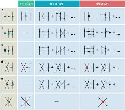
Figure 3: Chiral expansion of the $3N$F. Solid and dashed lines refer to nucleons and pions, respectively. Diagrams in the leftmost column visualize the two-pion exchange (a), two-pion-one-pion exchange (b), ring (c), one-pion-contact (d), two-pion-contact (e) and purely contact (f) $3N$F topologies. Cyan circles and ellipses in these diagrams represent scattering amplitudes of the corresponding sub-processes. The second, third and fourth columns show examples of diagrams, which contribute to the individual $3N$F topologies at increasing orders of the ChEFT expansion. Here, solid dots, filled circles and filled squares denote vertices from the effective Lagrangian of increasing chiral dimension $\Delta$ as explained in the text. Vertices shown in red involve LECs that need to be determined from three- or more-nucleon data.

In this figure, solid dots, filled circles and filled squares denote vertices from the effective Lagrangians of the dimension $\Delta=0$, $\Delta=1$ and $\Delta=2$, respectively, defined as $\Delta=d+\frac{1}{2}n-2$ with $d$ being the number of derivatives or $M_{\pi}$-insertions and $n$ the number of nucleon fields Weinberg:1990rz .

The leading $3N$F contributions arise at N²LO from tree-level diagrams contributing to the topologies (a), (d) and (f), which are made out of the $\Delta=0$-vertices and a single insertion of a $\Delta=1$ interaction Weinberg:1992yk ; kolk1994 . The short-range topologies (d) and (f) depend on the LECs $c_{D}$ and $c_{E}$, respectively, which cannot be fixed in the $NN$ system.

The first corrections to the leading $3N$F are generated by one-loop graphs made out of the lowest-order vertices with $\Delta=0$, see the third column in Fig. 3 for representative examples. Here, the shown diagrams represent sets of irreducible time-ordered-like graphs, whose precise meaning (and the corresponding algebraic expressions) depend on the employed choice for the off-shell part of the $NN$ and $3N$ potentials. For example, the $3N$F from the first of the two three-pion exchange diagrams of type (c) depends on the (ambiguous) choice made for the $1/m_{N}^{2}$-correction to the OPE $NN$ potential and the $1/m_{N}$-corrections to the tree-level two-pion exchange $3N$F of type (a), which appear at the same order.

The N³LO contribution to the longest-range topology (a) was derived in Ref. Ishikawa:2007zz based on the order-$Q^{3}$ $\pi N$ amplitude. These results were confirmed using the MUT in Ref. Bernard:2007sp , where also the expressions for the topologies (b) and (c) were derived. The shorter-range $3N$Fs of type (d) and (e), along with the $1/m_{N}$-corrections to the topologies (c) and (d), are worked out in Ref. Bernard:2011zr . All results mentioned above are obtained using dimensional regularization (DimReg) to evaluate divergent loop integrals and are parameter-free. Finally, it is worth mentioning that one can also draw tree-level $3N$ diagrams constructed from the leading $\Delta=0$-vertices and a single insertion of a $\Delta=2$-interaction from $\mathcal{L}_{\pi N}^{(3)}$ that could potentially contribute to the $3N$F at N³LO. However, all irreducible contributions generated by such diagrams either contribute to renormalization of the $\pi N$ coupling constant or vanish.

Subleading corrections to the $3N$F at N⁴LO are visualized in the last column of Fig. 3 and comprise one-loop diagrams made out of the leading $\Delta=0$-vertices and a single insertion of a $\Delta=1$-interaction from $\mathcal{L}_{\pi N}^{(2)}$, as well as tree-level graphs from the lowest-order interactions and a single insertion of a $\Delta=3$-vertex. The longest-range two-pion exchange $3N$F and the intermediate-range N⁴LO contributions of types (b), (c) are derived using the MUT in Refs. Krebs:2012yv and Krebs:2013kha , respectively. The corresponding potentials do not involve any unknown LECs. Short-range $3N$F terms of type (f) are considered in Ref. Girlanda:2011fh and depend on $13$ unknown LECs. Finally, one-loop contributions to the topologies (d) and (e) at N⁴LO are still to be worked out (and involve further unknown LECs).

In addition to the isospin-invariant $3N$F contributions discussed above and depicted in Fig. 3, one also has to account for isospin-breaking corrections stemming from different masses of the up and down quarks and QED effects. The expressions for isospin-violating $3N$F up through N⁴LO are worked out using the MUT in Ref. Epelbaum:2004xf , see also Ref. Friar:2004ca for a related work. Charge-dependent $3N$Fs involving virtual photon exchange are considered in Refs. Yang:1979zz ; Yang:1983pd and found to be rather weak. Parity- and time-reversal-violating $3N$Fs have also been studied, see the review article deVries:2020iea and references therein.

To demonstrate the predictive power of ChEFT we consider below the chiral expansion of the longest-range two-pion exchange $3N$F topology (a) as a representative example. We restrict ourselves to isospin-invariant contributions in the static limit, whose most general structure is given by

$$V^{(a)}_{3N} = \frac{\vec{\sigma}_{1}\cdot\vec{q}_{1}\,\vec{\sigma}_{3}\cdot\vec{q}_{3}}{(q_{1}^{2}+M_{\pi}^{2})\,(q_{3}^{2}+M_{\pi}^{2})}$$ (6)

$$\times \Big{[}\mbox{\boldmath$\tau$}_{1}\cdot\mbox{\boldmath$\tau$}_{3}\,{\cal A}(q_{2})+\mbox{\boldmath$\tau$}_{1}\times\mbox{\boldmath$\tau$}_{3}\cdot\mbox{\boldmath$\tau$}_{2}\,\vec{q}_{1}\times\vec{q}_{3}\cdot\vec{\sigma}_{2}\,{\cal B}(q_{2})\Big{]}$$

$$+ \text{ short-range terms}\;+\;\text{permutations}\,,$$

where the functions ${\cal A}$ and ${\cal B}$ depend on the momentum transfer $q_{2}\equiv|\vec{q}_{2}|$ of the second nucleon. These functions govern the long-distance behavior of the $3N$F and are to be determined by means of the chiral expansion

$${\cal A}(q_{2}) = {\cal A}_{[Q^{3}]}(q_{2})+{\cal A}_{[Q^{4}]}(q_{2})+{\cal A}_{[Q^{5}]}(q_{2})+\ldots,$$

$${\cal B}(q_{2}) = {\cal B}_{[Q^{3}]}(q_{2})+{\cal B}_{[Q^{4}]}(q_{2})+{\cal B}_{[Q^{5}]}(q_{2})+\ldots.$$ (7)

The dominant contributions to ${\cal A}(q_{2})$ and ${\cal B}(q_{2})$ at N²LO, stemming from the tree diagram in the second column of Fig. 3, have the form Epelbaum:2002vt ; kolk1994

$${\cal A}_{[Q^{3}]} = \frac{g_{A}^{2}}{8F_{\pi}^{4}}\Big{[}(2c_{3}-4c_{1})M_{\pi}^{2}+c_{3}q_{2}^{2}\Big{]},$$

$${\cal B}_{[Q^{3}]} = \frac{g_{A}^{2}c_{4}}{8F_{\pi}^{4}},$$ (8)

where $c_{i}$ denote the $\pi N$ LECs from the subleading Lagrangian $\mathcal{L}_{\pi N}^{(2)}$.

The leading corrections to Eq. (2.2.4) are generated at N³LO by one-loop diagrams shown in the first line and third column of Fig. 3. Using DimReg, one obtains Bernard:2007sp ; Ishikawa:2007zz

$${\cal A}_{[Q^{4}]} = \frac{g_{A}^{4}}{256\pi F_{\pi}^{6}}\Big{[}\left(4g_{A}^{2}+1\right)M_{\pi}^{3}+2\left(g_{A}^{2}+1\right)M_{\pi}q_{2}^{2}$$ (9)

$$+ A(q_{2})\left(2M_{\pi}^{4}+5M_{\pi}^{2}q_{2}^{2}+2q_{2}^{4}\right)\Big{]},$$

$${\cal B}_{[Q^{4}]} = -\frac{g_{A}^{4}}{256\pi F_{\pi}^{6}}\big{[}A(q_{2})\left(4M_{\pi}^{2}+q_{2}^{2}\right)+(2g_{A}^{2}+1)M_{\pi}\big{]},$$

where we have introduced the loop function

$$A(q_{2})=\frac{1}{2q_{2}}\arctan\frac{q_{2}}{2M_{\pi}}.$$ (10)

The loop function $A(q_{2})$ possesses a left-hand cut with the branch point at $q_{2}^{2}=-(2M_{\pi})^{2}$, which corresponds to the kinematics when both pions inside the loop of, e.g., the first N³LO diagram can become on-shell. On the other hand, contributions from diagrams like the second N³LO graph do not have left-hand cuts and are polynomial in $q_{2}^{2}$. Notice further that loop integrals at N³LO involve only linear divergences, which vanish in DimReg (and would have been absorbed into the LEC $c_{D}$ when using momentum-dependent regularization schemes). This is consistent with the already mentioned absence of tree-level $3N$F contributions involving a single insertion from $\mathcal{L}_{\pi N}^{(3)}$.

Finally, the N⁴LO result for the functions ${\cal A}(q_{2})$ and ${\cal B}(q_{2})$, obtained using DimReg, has the form Krebs:2012yv

$${\cal A}_{[Q^{5}]} = \frac{g_{A}^{2}\bar{e}_{14}}{2F_{\pi}^{4}}\big{(}2M_{\pi}^{2}+q_{2}^{2}\big{)}^{2}+\frac{g_{A}^{2}\big{(}M_{\pi}^{2}+2q_{2}^{2}\big{)}}{4608\pi^{2}F_{\pi}^{6}}$$

$$\times \Big{\{}\big{[}6c_{1}-2c_{2}-3c_{3}-2(6c_{1}-c_{2}-3c_{3})L(q_{2})\big{]}$$

$$\times 12M_{\pi}^{2}-q_{2}^{2}\big{[}5c_{2}+18c_{3}-6L(q_{2})(c_{2}+6c_{3})\big{]}\Big{\}},$$

$${\cal B}_{[Q^{5}]} = \frac{g_{A}^{2}\bar{e}_{17}}{2F_{\pi}^{4}}\big{(}2M_{\pi}^{2}+q_{2}^{2}\big{)}\;-\;\frac{g_{A}^{2}c_{4}}{2304\pi^{2}F_{\pi}^{6}}$$

$$\times \Big{\{}q_{2}^{2}\big{[}5-6L(q_{2})\big{]}+12M_{\pi}^{2}\big{[}2+9g_{A}^{2}-2L(q_{2})\big{]}\Big{\}},$$

where $\bar{e}_{14}$ and $\bar{e}_{17}$ are renormalized LECs from $\mathcal{L}_{\pi N}^{(4)}$, evaluated in the $\overline{\rm MS}$ scheme with the renormalization scale $\mu$ set to $\mu=M_{\pi}$. Further, the loop function $L(q_{2})$ is given by

$$L(q_{2})=\frac{\sqrt{q_{2}^{2}+4M_{\pi}^{2}}}{q_{2}}\log\frac{\sqrt{q_{2}^{2}+4M_{\pi}^{2}}+q_{2}}{2M_{\pi}},$$ (12)

and it also possesses a left-hand cut that starts at $q_{2}^{2}=-(2M_{\pi})^{2}$. Notice that in Eq. (2.2.4), we have applied the shifts of the LECs $c_{i}$ specified in Eq. (16) of Ref. Siemens:2016hdi to eliminate certain redundant linear combinations of LECs.

Given that all LECs entering Eqs. (2.2.4)-(2.2.4) are known from $\pi N$ scattering, which serves as a sub-process for the $3N$F topology (a), the above expressions for ${\cal A}(q_{2})$ and ${\cal B}(q_{2})$ are to be regarded as parameter-free predictions of ChEFT. To assess the convergence of the chiral expansion for the longest-range $3N$F, we employ the numerical values for the pion mass and decay constant of $M_{\pi}=138.03$ MeV and $F_{\pi}=92.2$ MeV. The nucleon axial coupling $g_{A}$ is set to the effective value of $g_{A}=1.289$ that accounts for the Goldberger-Treiman discrepancy. The most reliable values of the higher-order $\pi N$ LECs are obtained from matching ChPT with the solution of the dispersive Roy-Steiner equations for $\pi N$ scattering at the subthreshold kinematical point, see Refs. Siemens:2016jwj ; Hoferichter:2015tha for details. In the following, we employ the central values from the order-$Q^{4}$ heavy-baryon-NN fit of Ref. Siemens:2016jwj : $c_{1}=-1.11$, $c_{2}=3.61$, $c_{3}=-5.60$, $c_{4}=4.26$, $\bar{e}_{14}=1.16$ and $\bar{e}_{17}=-0.17$. Here, the values of $c_{i}$ and $\bar{e}_{i}$ are given in units of GeV^-1 and GeV^-3, respectively.

In Fig. 4, we show the predicted behavior of the functions ${\cal A}(q_{2})$ and ${\cal B}(q_{2})$ at different orders in ChEFT.

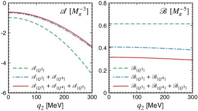
Figure 4: ChEFT predictions for the functions ${\cal{A}}(q_{2})$ and ${\cal{B}}(q_{2})$ that parametrize the longest-range behavior of the $3N$F according to Eq. (6). Green dashed, blue dashed-dotted and red solid lines show the results at N²LO, N³LO and N⁴LO, respectively.

In both cases, the order-$Q^{4}$ corrections to the dominant order-$Q^{3}$ contributions amount to about $30\%$. The order-$Q^{5}$ correction is very small for ${\cal{A}}(q_{2})$ and amounts to less than $15\%$ of the N²LO result for the function ${\cal{B}}(q_{2})$. The observed convergence pattern for ${\cal{A}}(q_{2})$ and ${\cal{B}}(q_{2})$ fits well with expectations based on the power counting with the expansion parameter $Q\sim{\rm max}(M_{\pi},q_{2})/\Lambda_{b}$, see also the discussion in Sec. 2.2.3, and shows that the low-momentum structure of the $3N$F can be described in ChEFT in a controlled and systematically improvable fashion. Notice that in addition to the static contributions considered above, the $3N$F of type (a) at N³LO receives non-local $1/m_{N}$ corrections of relativistic origin Bernard:2011zr . These have a much richer operator structure than the static terms and also do not involve unknown LECs.

Parameter-free predictions for the one-pion-two-pion exchange and ring $3N$F topologies corresponding to diagrams (b) and (c) in Fig. 3 can be found in Refs. Bernard:2007sp ; Krebs:2013kha and follow a qualitatively similar pattern. We also emphasize that while the static two-pion exchange $3N$F has a rather restricted form described by just two functions, the long-and intermediate-range topologies (a), (b) and (c) contribute to all $20$ operators $\hat{O}_{\alpha}$ that appear in the parametrization of the $3N$F according to Eq. (5). Interestingly, the results for the corresponding functions $f_{\alpha}$ appear to be qualitatively in line with estimations based on the large-$N_{c}$ expansion in QCD Phillips:2013rsa ; Epelbaum:2014sea .

As pointed out in the introduction, an intermediate excitation of the nucleon into the $\Delta(1232)$ resonance was historically recognized as one of the most important $3N$F mechanisms and is at the heart of the celebrated Fujita-Miyazawa $3N$F model 10.1143/PTP.17.360 as depicted in Fig. 1. How can this important phenomenological insight be reconciled with the framework of ChEFT? All results discussed in this section are obtained using the ChEFT formulation with pions and nucleons as the only explicit degrees of freedom in the effective Lagrangian. In such a framework, the information about the $\Delta$ resonance is included implicitly through its contributions to various LECs. In particular, the LECs $c_{i}$ are largely governed by the $\Delta$ resonance Bernard:1996gq :

$$c_{2}^{\Delta}=-c_{3}^{\Delta}=2c_{4}^{\Delta}=\frac{4h_{A}^{2}}{9(m_{\Delta}-m_{N})}\simeq 2.7\;\text{GeV}^{-1}\,,$$ (13)

where $m_{\Delta}$ refers to the mass of the $\Delta$ resonance while $h_{A}\sim 1.34$ is the $N\Delta$ axial coupling constant. Thus, the $\Delta$ largely saturates the LECs $c_{2}$ and $c_{4}$, and provides about a half of the $c_{3}$-value, thereby offering an explanation of the somewhat large numerical values of these LECs as compared with their expected size $|c_{i}|\sim\Lambda_{b}^{-1}$. This confirms that the intermediate $\Delta$ excitation indeed provides the dominant mechanism of the two-pion exchange $3N$F through Eqs. (2.2.4) and (13).

Given the strong coupling of the $\Delta$ isobar to the $\pi N$ system and the smallness of the mass difference $m_{\Delta}-m_{N}$, which is numerically of the order of $2M_{\pi}$, it may be advantageous to include the $\Delta$ isobar as an explicit degree of freedom in the effective Lagrangian instead of integrating it out assuming $m_{\Delta}-m_{N}\sim\Lambda_{b}$, as done in the standard formulation of ChEFT. In the $\Delta$-full formulation of ChPT of Ref. Hemmert:1997ye , the mass difference $m_{\Delta}-m_{N}$ is treated as an additional soft scale $m_{\Delta}-m_{N}\sim M_{\pi}$ (in spite of the fact that this quantity does not vanish in the chiral limit). Accordingly, the $\Delta$ isobar is treated explicitly in the effective Lagrangian, and the new expansion parameter is denoted as $\epsilon\in\{p/\Lambda_{b},M_{\pi}/\Lambda_{b},(m_{\Delta}-m_{N})/\Lambda_{b}\}$. Extensive studies in the single-nucleon sector using manifestly covariant formulations of ChPT have revealed that the explicit treatment of the $\Delta$ isobar indeed often leads to an improved convergence of the EFT expansion, see e.g. Refs. Siemens:2016hdi ; Yao:2016vbz ; HillerBlin:2014diw ; Thurmann:2020mog , albeit at the cost of more involved calculations and a larger number of LECs. Similar conclusions have been reached for the $NN$ force using the heavy-baryon formulation of $\Delta$-full ChEFT, for which the expressions are presently available up through N²LO $\epsilon^{3}$ Ordonez:1995rz ; Kaiser:1998wa ; Krebs:2007rh . Isospin-breaking contributions to the $NN$ potential have also been considered within the $\epsilon$-expansion scheme Epelbaum:2008td .

The explicit treatment of the $\Delta$ isobar also has implications for the $3N$F. In particular, the dominant Fujita-Miyazawa-type contribution is shifted from N²LO to NLO in the $\Delta$-full scheme, since the diagram in Fig. 1 counts as of order $\epsilon^{2}$. Interestingly, this is the only contribution of the $\Delta$ to the $3N$F up-to-and-including the order N²LO (i.e., $\epsilon^{3}$) Epelbaum:2007sq . Recently, the longest-range $3N$F of type (a) in Fig. 3 has been worked out at order $\epsilon^{4}$ Krebs:2018jkc . The resulting parameter-free predictions were found to agree well with the order-$Q^{5}$ results of Ref. Krebs:2012yv , which shows that the effects of the $\Delta$ are well captured by resonance saturation of the $\pi N$ LECs in the $\Delta$-less ChEFT framework and suggests that convergence might have been reached for this topology. The corresponding results for the intermediate-range $3N$F of types (b) and (c) within the $\epsilon$-expansion are not yet available. Notice that in the $\Delta$-less scheme, the first information about the $\Delta$ isobar for these topologies appears only at N⁴LO, since the N³LO expressions depend solely on the LO LECs, see e.g. Eq. (9), which contain no information about the $\Delta$ isobar. The explicit inclusion of the $\Delta$ might, therefore, be advantageous to achieve convergence for these topologies.

So far we have left open the question of regularization of the $3N$F. As already pointed out in Sec. 2.2.2, ChEFT allows one to derive low-momentum approximations of the nuclear forces, but the method looses its validity for large momenta $|\vec{p}\,|\gtrsim\Lambda_{b}$. For example, the ChEFT predictions for the function ${\cal{A}}(q_{2})$ in Eqs. (2.2.4), (9) and (2.2.4) behave at large $q_{2}$-values as ${\cal{A}}_{[Q^{3}]}(q_{2})\sim q_{2}^{2}$, ${\cal{A}}_{[Q^{4}]}(q_{2})\sim q_{2}^{3}$ and ${\cal{A}}_{[Q^{5}]}(q_{2})\sim q_{2}^{4}\,\log(q_{2})$, respectively. While the expansion for ${\cal{A}}(q_{2})$ appears to converge well within the applicability range of ChEFT, with the order-$Q^{5}$ result providing a tiny correction as shown in the left panel of Fig. 4, the N⁴LO contribution starts exceeding the N³LO correction at $q_{2}\sim 780$ MeV, signalling the breakdown of the expansion at large momenta. As explained in Sec. 2.2.2, the expressions for nuclear forces derived in ChEFT have to be regularized by introducing a finite cutoff $\Lambda\sim\Lambda_{b}$ to remove their uncontrolled behavior at large momenta and make the $A$-body Schrödinger equation well defined. In the $NN$ sector, this can be achieved, e.g., by simply multiplying the unregularized potentials with some regulator functions. Unfortunately, following this same strategy for the $3N$F was found in Refs. Epelbaum:2019kcf ; Epelbaum:2019jbv ; Epelbaum:2022cyo to violate the chiral symmetry. The problem can be best illustrated with the $3N$F of type (b) stemming from the first of the two diagrams shown in the second line and third column of Fig. 3. When calculating the scattering amplitude, the irreducible $3N$F is supplemented with the corresponding reducible contributions stemming from the iteration of the Faddeev equation. This reducible contribution involves a linearly divergent piece $\propto\Lambda$, whose structure violates the chiral symmetry. Accordingly, the amplitude cannot be renormalized by re-adjusting the LEC $c_{D}$, and the whole ChEFT expansion for $3N$ scattering breaks down. As explained in Refs. Epelbaum:2019kcf ; Epelbaum:2019jbv ; Epelbaum:2022cyo , the problem is caused by mixing of two different regularization schemes, namely DimReg when deriving the $3N$F and cutoff regularization in the Schrödinger equation. The same issue affects loop contributions to the nuclear current operators Krebs:2019ddp ; Krebs:2020pii . This shows that a consistent regularization of the $3N$F and nuclear currents cannot be achieved by simply multiplying the corresponding potentials derived using DimReg with some cutoff functions. Rather, $3N$Fs, 4NFs and nuclear currents starting from N³LO need to be re-derived using a cutoff instead of DimReg.

The above conceptual issues have been the main obstacle for the applications of ChEFT to three- and more-nucleon systems beyond N²LO. In contrast to DimReg, maintaining the chiral and gauge symmetries in cutoff regularization represents a non-trivial task, and the calculations become considerably more involved due to the appearance of an additional mass scale $\Lambda$. Recently, it was shown that the symmetry-preserving gradient flow method, which has been successfully applied to Yang-Mills theories Luscher:2011bx ; Luscher:2013cpa and is nowadays widely employed in lattice-QCD simulations Luscher:2013vga , can be merged with ChEFT Krebs:2023gge and applied to obtain consistently regularized nuclear forces and currents Krebs:2023ljo . This is achieved by generalizing the pion fields to the (artificial) fifth dimension, usually referred to as the flow “time” $\tau$. The flow-time evolution of the pion fields is governed by the chirally covariant version of the gradient flow equation and amounts to smothening of the pion field, i.e., a non-zero flow time $\tau$ acts as a regulator. Moreover, when applied to the OPEP, the gradient flow method reduces to the SMS regulator of Ref. Reinert:2017usi specified in Eq. (3). The new developments in Refs. Krebs:2023gge ; Krebs:2023ljo lay down the foundation for deriving consistently regularized $3N$F and nuclear currents beyond N²LO. Work along these lines is in progress.

2.2.5 Selected applications of the lading $3N$F

We now turn to applications of the chiral nuclear forces to the 3N and heavier systems, focusing especially on the role of $3N$Fs. Given the lack of consistently regularized $3N$Fs at N³LO and N⁴LO as described in the previous section, the accuracy level of the applications reviewed below is limited to N²LO.

Nucleon-deuteron ($Nd$) elastic scattering and breakup observables can be calculated, starting from a given nuclear Hamiltonian, by solving the Faddeev equations in the partial wave basis as described in detail in the review article Gloeckle:1995jg . $Nd$ scattering calculations described below are carried out without explicit inclusion of the Coulomb interaction and neglecting relativistic effects, which are known to be small al low and intermediate energies Witala:2004pv ; Witala:2011yq . We also restrict ourselves to studies based on the second-generation of chiral $NN$ potentials introduced in Refs. Epelbaum:2014efa ; Epelbaum:2014sza ; Reinert:2017usi , see Refs. epelbaum2009 ; Epelbaum:2005pn ; Kalantar-Nayestanaki_2012 ; Epelbaum:2012vx ; Hammer:2012id and references therein for earlier studies along this line. The novel semi-local regularization method employed in these NN potentials allows one to avoid the appearance of noticeable artifacts in elastic $Nd$ scattering at large energies reported in Ref. Witala:2013ioa for the first-generation of N³LO chiral $NN$ potentials of Refs. Epelbaum:2004fk ; Entem:2003ft , which can be traced back to the artifacts in the deuteron wave function. The novel semi-local potentials thus provide a very good starting ground for systematic studies of $Nd$ scattering in ChEFT.

In a series of papers by the LENPIC Collaboration, the semi-local coordinate-space regularized (SCS) $NN$ potentials of Refs. Epelbaum:2014efa ; Epelbaum:2014sza at all available orders from LO to N⁴LO were employed to calculate $Nd$ scattering observables and properties of selected nuclei up to ⁴⁸Ca LENPIC:2015qsz ; Maris:2016wrd ; LENPIC:2018lzt . While these calculations did not include the $3N$F and thus should be regarded as incomplete starting from N²LO, they have yielded a number of interesting observations. In particular, calculations beyond the last complete order NLO were found to differ from experimental data well outside the estimated truncation uncertainties, thus providing unambiguous evidence for missing $3N$Fs. Moreover, the amount of deviations between theory and experimental data was found to be consistent with estimations based on the power counting.

In Ref. LENPIC:2018ewt , these studies have been extended to include the N²LO $3N$F, regularized in coordinate space consistently with the SCS $NN$ potentials. The need to perform regularization of the $3N$F in coordinate space was found to introduce significant computational overhead for its numerical implementation, which was one of the motivations to reformulate the SCS regularization scheme to momentum space Reinert:2017usi . Notice that partial wave decomposition of a general $3N$F can be carried out in an automated way by numerically performing the required angular integrations as described in Refs. Golak:2009ri ; Hebeler:2015wxa , see also Ref. PhysRep21Hebeler .

As detailed in Sec. 2.2.4, the $3N$F at N²LO depends on the LECs $c_{D}$ and $c_{E}$ that need to be determined from few-nucleon data. It is customary to fix the linear combination of these LECs to reproduce the ³H binding energy, which determines $c_{E}$ as a function of $c_{D}$. To fix the second LECs, different observables have been proposed in the literature including the Nd doublet scattering length Epelbaum:2002vt ; Piarulli:2017dwd , ³H beta decay Gazit:2008ma , ⁴He binding energy Nogga:2005hp , charge radii of the $A=3,4$ nuclei and properties of few- and many-nucleon systems Navratil:2007we ; Ekstrom:2015rta ; Lynn:2017fxg . Clearly, to allow for the most stringent test of the nuclear Hamiltonian, the LECs should ideally be fixed from $A\leq 3$ observables. In Ref. LENPIC:2018ewt , a variety of observables including the Nd doublet scattering length as well as the Nd total and differential cross sections at the energies of $E_{\rm lab}=70$, $108$ and $135$ MeV have been considered. Taking into account both the experimental errors and the EFT truncation uncertainty, the strongest constraint on $c_{D}$ was found to result from the requirement to reproduce the proton-deuteron (pd) differential cross section minimum using the data from Ref. sekiguchi2002 . The resulting Hamiltonian was then used to calculate $Nd$ elastic scattering observables, ground state energies and selected excitation energies of $p$-shell nuclei up to ¹²C. For almost all considered nuclei, adding the $3N$F was found to significantly improve the description of experimental data. A detailed analysis of elastic $Nd$ scattering and breakup using the same Hamiltonian is presented in Ref. Witala:2019ffj .

These studies were further refined in Ref. Maris:2020qne by employing the high-precision SMS $NN$ interactions of Ref. Reinert:2017usi along with the consistently regularized N²LO $3N$Fs, utilizing Bayesian methods for quantifying EFT truncation errors and extending the range of considered observables.

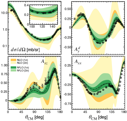
Figure 5: ChEFT predictions for the differential cross section, deuteron vector analyzing power $A_{y}^{d}$ and deuteron tensor analyzing powers $A_{xz}$ and $A_{xx}$ in elastic neutron-deuteron scattering at $E_{\rm lab}=135$ MeV. Dark-shaded orange and green bands show the NLO and N²LO results at the $1\sigma$ confidence level, respectively, while the corresponding light-shaded bands show the $2\sigma$-intervals. Experimental data are pd elastic scattering data from Ref. sekiguchi2002 . Dashed lines in the middle of green bands are the actual N²LO predictions. Dotted lines are obtained using the NN interaction at the highest available order N⁴LO⁺, supplemented with the N²LO $3N$F (with the appropriately re-adjusted LECs $c_{D}$ and $c_{E}$). In all calculations, the cutoff is chosen to be $\Lambda=450$ MeV.

In Fig. 5, we show selected results for $Nd$ elastic scattering observables at $E_{\rm lab}=135$ MeV, which may serve as representative examples. Given that the LECs $c_{D}$ and $c_{E}$ are fixed from the ³H binding energy and the differential cross section minimum at $E_{\rm lab}=70$ MeV, the shown results are to be regarded as predictions. The experimental data from Ref. sekiguchi2002 are mostly in agreement with the calculations (within errors), but the N²LO truncation uncertainty at this moderate energy appears to be rather large. The description of $Nd$ data at N²LO is qualitatively similar to the one for proton-proton scattering as a comparable energy, shown in Fig. 2. Based on the results in the $NN$ system, it is expected that taking into account the $3N$F up through N⁴LO would allow one to achieve a precise description of $Nd$ scattering data, comparable to that of the neutron-proton and proton-proton data reported in Refs. Reinert:2017usi ; Reinert:2020mcu .

It is interesting to explore the impact of corrections to the $NN$ force beyond N²LO. To this aim, a set of calculations based on the SMS NN potentials up through N⁴LO⁺, supplemented with the N²LO $3N$F, has been performed in Ref. LENPIC:2022cyu . In all cases, the LECs $c_{D}$ and $c_{E}$ have been fixed following the standard LENPIC fitting protocol described above. For the considered $Nd$ scattering observables, the inclusion of corrections to the NN force beyond N²LO changes the central N²LO predictions, shown by the dashed lines in Fig. 5, to the dotted lines. The results visualized by the dashed and dotted lines differ by N³LO terms, and it is comforting to see that the differences between these lines are within the estimated N²LO truncation errors. While the higher-order corrections to the $NN$ force do appear to noticeably improve the description of the tensor analyzing powers $A_{xz}$ and $A_{xx}$ in the angular range of $\theta_{\rm CM}\in[45^{\circ},100^{\circ}]$, they still leave room for improvement that should come from higher-order contributions to the $3N$F.

Further, we mention a comprehensive study of the symmetric space-star deuteron breakup configuration in Ref. Witala:2021zmb . This particular configuration is known to exhibit large discrepancies between theory and data at energies below $E_{\rm lab}\sim 25$ MeV that could so far not be resolved. Moreover, the calculated cross section appears to be largely insensitive to the types of $3N$F considered so far. It would be interesting to study the impact of $3N$F contributions beyond N²LO on this observable. Finally, a detailed investigation of the deuteron breakup reaction at $E_{\rm lab}\sim 130$ and $200$ MeV using the chiral SMS $NN$ and $3N$-forces and covering the whole kinematically allowed phase space has been carried out in Ref. Skibinski:2023nnn .

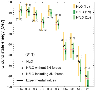
Figure 6: ChEFT predictions for the ground state energies of light nuclei calculated using the No-Core Configuration Interaction (NCCI) method Barrett:2013nh . Crosses, circles and diamonds show the NLO results, incomplete N²LO predictions using the $NN$ interactions only and the complete results at N²LO using both the $NN$ force and $3N$F. Orange, green dark-shaded and green light-shaded error bars show the NLO $(1\sigma)$, N²LO $(1\sigma)$ and N²LO $(2\sigma)$ ChEFT truncation errors, respectively, while black error bars give the numerical uncertainty of the NCCI method. All theoretical predictions are obtained using the cutoff value of $\Lambda=450$ MeV. Horizontal lines depict the experimental values for the binding energies. See Ref. Maris:2020qne for details.

In Fig. 6, we show the NLO and N²LO predictions for the ground-state energies of light $p$-shell nuclei from Ref. Maris:2020qne . For all nuclei, the predicted binding energies at both NLO and N²LO agree with experimental values within truncation errors. To facilitate the quantification of $3N$F effects, we also show the results based on the N²LO $NN$ potential without inclusion of the $3N$F. For light nuclei up to ¹⁰B, the inclusion of the $3N$F leads to a significant improvement. However, for both considered $A=12$-nuclei, the $3N$F effects appear to be too large leading to overbinding. This overbinding was shown in Ref. LENPIC:2022cyu to be resolved by taking into account the corrections to the $NN$ force beyond N²LO.

Last but not least, N⁴LO short-range contributions to the $3N$F have been considered in the exploratory studies of $Nd$ scattering reported in Refs. Girlanda:2018xrw ; Epelbaum:2019zqc ; Witala:2022rzl . While incomplete, these studies demonstrate that the N⁴LO contact interactions of natural size have the potential to both resolve the long-standing $A_{y}$-puzzle in low-energy elastic Nd scattering and strongly improve the description of scattering observables at high energies.

2.3 Experimental studies of three-nucleon forces

To uncover the structure of $3N$Fs one must utilize systems with more than two nucleons ($A>3$). Few-nucleon scattering offers a unique opportunity to probe dynamical aspects of $3N$Fs, which are momentum, spin and isospin dependent, since it provides not only the cross sections but also a variety of spin observables at different incident nucleon energies. A direct comparison between experimental data and rigorous numerical calculations using the Faddeev theory and based on the realistic nuclear potentials provides detailed information on the structure of $3N$Fs.

The importance of $3N$Fs in the continuum spectrum was shown, for the first time, in nucleon–deuteron ($Nd$) elastic scattering at the end of the 1990s wit98 . $3N$Fs were found to lead to pronounced effects around the cross-section minimum occurring at the values of the c.m. scattering angle of $\theta_{c.m.}\approx 120^{\circ}$ for incident energies above $60~{}\rm MeV/nucleon$. Since then, proton-deuteron($pd$) and neutron-deuteron($nd$) scattering experiments at 60–300 MeV/nucleon have been performed at the facilities, e.g. RIKEN, RCNP, KVI, IUCF, TSL, and LANSCE, providing precise data of the cross sections as well as various types of spin observables Kalantar-Nayestanaki_2012 .

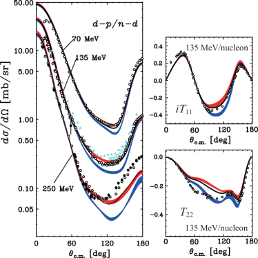
Figure 7: Differential cross section and deuteron analyzing powers $iT_{11}$, $T_{22}$ for elastic nucleon-deuteron scattering. See text for descriptions for the theoretical calculations.

Figure 7 shows some representative experimental results reported in Refs. sekiguchi2002 ; PhysRevLett.95.162301 ; PhysRevC.76.014004 ; PhysRevC.89.064007 ($dp$ or $pd$ in black open circles, $nd$ in black solid circles). Data shown in blue are from Refs. PhysRevC.68.051001 ; PhysRevC.78.014006 . The experimental data are compared with the Faddeev calculations with and w/o $3N$Fs. The red (blue) bands are the calculations with (without) Tucson-Melbourne 99 $3N$F based on the modern $NN$ potentials, i.e. CD Bonn, AV18, Nijmegen I and II. The solid lines are the calculations based on the AV18 potential with including the Urbana IX $3N$F. The $3N$Fs considered here are 2$\pi$–exchange types. For most of the observables shown in the figure, large differences are found at the backward angles between the data and the calculations based on $NN$ forces only. These discrepancies become larger with an increasing incident energy. For the cross section, the $3N$Fs remove the discrepancies at lower energies. At higher energies, however, the differences still remain even including the $3N$F potentials at the angles $\theta_{\rm c.m.}\gtrsim 120^{\circ}$, which extent to the very backward angles $\theta_{\rm c.m.}\sim 180^{\circ}$ at 250 MeV/nucleon. For the vector analyzing power $iT_{11}$, the description of the experimental data by the theoretical calculations is similar to that of the cross section. However, for the tensor analyzing power $T_{22}$ a different pattern is observed as the calculations including the $3N$Fs do not explain the data at the lower two energies.

A direct comparison between the data and the Faddeev calculations in elastic $Nd$ scattering led to the following conclusions so far: (1) the $3N$F is definitely needed in elastic $dp$ scattering; (2) the $3N$F effects are clearly seen at the angles where the cross section takes its minimum, and their effects become larger with an increasing incident energy; (3) spin dependent parts of the current $3N$F models are deficient; (4) the short-range components of the $3N$F are probably required for high-momentum transfer region (at the very backward angles). These results of comparison between the data and the calculations based on the above phenomenological nuclear potentials have been pushing into more detailed study of three-nucleon scattering based on the $\chi$EFT nuclear potential as described in Sec. 2.2.

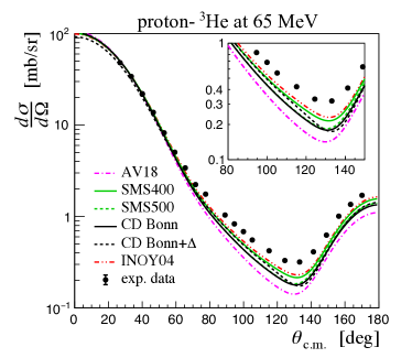
Figure 8: Experimental data (solid circles) and the calculations from the solutions of exact AGS equations of the differential cross section $d\sigma/d\Omega$ at 65 MeV for $p$-${}^{3}\rm He$ elastic scattering PhysRevC.103.044001 . Calculations based on the $NN$ potentials are shown with magenta dash-dotted (AV18), black solid (CD Bonn), red dot-dot-dashed (INOY04), green solid (SMS400), and green dashed (SMS500) lines. Black dashed lines are calculations based on the CD Bonn+potential.

It is important to keep in mind that the $Nd$ system is dominated by the isospin $T=1/2$ states. Thus, one needs other probes to constrain the properties of the $3N$Fs with total isospin $T=3/2$, whose importance is strongly suggested in the description of asymmetric nuclear matter, e.g. neutron-rich nuclei and pure neutron matter. Such aspects could be studied in four-nucleon systems like proton-$\rm{}^{3}He$. In recent years, remarkable theoretical progress in solving the 4N scattering problem using realistic Hamiltonians has been reported Deltuva_PRC76 ; lazauskas2009 ; viviani_PRL111 even above the 4N breakup threshold deltuva_prc87 ; fonseca_FBS2017 , opening new possibilities for nuclear force study in the 4N system at intermediate energies. In Fig. 8 the recent results of $p$-${}^{3}\rm He$ scattering at intermediate energy are presented PhysRevC.103.044001 . The cross section data at 65 MeV/nucleon are compared with the calculations from the solutions of the exact AGS equations as given in Refs. deltuva_prc87 ; fonseca_FBS2017 using a variety of $NN$ potentials: the AV18, the CD Bonn, and the INOY04 INOY04 , and the chiral N4LO $NN$ potentials with the cutoff parameters $\Lambda$ = 400 ${\rm MeV}/c$ (SMS400) and $\Lambda=500{\rm MeV}/c$ (SMS500)  SMS . The calculations based on the CD Bonn+$\Delta$ model CDBD , which allows an excitation of a nucleon to an isobar, thereby providing effective $3N$Fs and $4N$Fs, are also presented. Large contributions of the effective $3N$ and $4N$ forces have been found to be largely canceled by the dispersive isobar effect, leading to rather small total contributions from the $\Delta$-isobar. The results are in contrast to those in $dp$ scattering, where the cancellation is less pronounced Nemoto1999 . The obtained results indicate that $p$-${}^{3}\rm He$ elastic scattering at intermediate energies is an excellent tool to explore nuclear interactions including $3N$Fs, which cannot be accessed in $3N$ scattering. It would be interesting to see how the predictions with such $3N$Fs explain the data for the $p$-${}^{3}\rm He$ elastic scattering, which will enable us to perform detailed discussions of the effects of $3N$Fs including the $T=3/2$ isospin channels.

3 Three-body forces in atoms

Cold atoms are systems of dilute atomic gases cooled down to nano-Kelvin temperatures. While the interactions among atoms are dominated by two-body forces and their intrinsic three-body forces are negligible, one can engineer and realize cold atoms with an effective three-body force as strong as or even stronger than the two-body force, capitalizing on the high controllability of cold-atom experiments gross2017quantum ; schafer2020tools . In this section, we overview recent experimental and theoretical attempts to observe, control, and utilize three-body forces in cold atoms.

3.1 Experimental observations of three-body forces for cold atoms in an optical lattice

A system of cold atoms such as a Bose-Einstein condensate (BEC) or a Fermi-degenerate gas loaded into an optical lattice is known to be an ideal experimental platform for the quantum simulation of strongly-correlated quantum many-body systems bloch_many-body_2008 , such as the Hubbard model, owing to the high controllability of its parameters like hopping energy and on-site interaction, and so on. When cold atoms are trapped in a sufficiently deep optical lattice potential, the hopping between neighboring lattice sites is negligible. This gives us a novel possibility to simultaneously realize various well-defined few-body systems with definite atom numbers. Under these conditions, the trapping potential for the atoms in each lattice site is well approximated by a harmonic potential. Therefore, a system of cold atoms in an optical lattice is also a useful platform for studying few-body physics in a trap.

Various spectroscopic techniques have been developed in cold atoms, which are quite useful to probe the energy of these few-body systems. The first occupancy-resolved high-resolution spectroscopy was reported for a radio-frequency spectroscopy of the ground hyperfine states of rubidium atoms Campbell2006 . The observed almost equi-distance between the neighboring resonance frequencies is explained by the pairwise interactions alone. However, slight deviation of the equi-distance between the neighboring resonance frequencies was also observed, indicating that the simple pairwise interaction is insufficient. The qualitative explanation in the microscopic description of the system was given as the broadening of the Wannier function due to the two-body interaction. Similar observations of the slight deviation from the prediction based on the pairwise interaction were reported in the experiments using various methods like matter-wave collapse and revival measurement Will2010 , resonant lattice modulation PhysRevLett.107.175301 , and laser spectroscopy Franchi_2017 ; Goban2018 . This deviation is successfully explained by introducing an effective three-body force between the trapped atoms within perturbative treatments Johnson_2009 ; Johnson_2012 . Interestingly, the microscopic origin of the effective three-body force, where one of the three atoms in the lowest vibrational state is excited to the higher vibrational state due to the inter-atomic interaction with the second atom and then is returned to the lowest state via the inter-atomic interaction with the third atom, has close analogy with the Fujita-Miyazawa type nuclear three-body force discussed in Sec. 1 10.1143/PTP.17.360 (compare Fig. 1 with Fig. 9 in the next subsection).

Here, we stress that the three-body forces in the nuclear and trapped-atom systems share the same grounds in that they are the effective forces which are considered in low-energy effective descriptions of the systems. The cold-atom system can be a useful testbed to explore the three-body forces, firstly because of its high controllability, and secondly because the intrinsic three-body force between atoms is so small that we can directly investigate the physical mechanism for the emergence of the effective three-body forces.

Following this line of research direction, an occupancy-resolved high-resolution laser spectroscopy has been performed in recent experiments to investigate a new regime of three-body force honda2024evidence . In particular, by working with the ultra-narrow optical transition between the ground ${}^{1}S_{0}$ and metastable ${}^{3}P_{2}$ states of ytterbium (Yb) atoms PhysRevLett.110.173201 , one can utilize both the high resolution in the determination of the binding energy of the few-body atomic system and the high controllability of the two-body interaction through an inter-orbital anisotropy-induced Feshbach resonance Chin2010 . This enables us to study a new regime of three-body force beyond the perturbative treatment in the weakly-interacting regime. While the data at small scattering lengths far from the Feshbach resonance are well explained by perturbative calculations, as in the previous works, the results obtained around the Feshbach resonance show significantly different behaviors from the equi-distance between the neighboring resonance frequencies, indicating a strongly-interacting regime of three-body forces, owing to the resonant control of the two-body interaction honda2024evidence . These results obtained by a cold-atom quantum simulator with tunable interactions can be a useful benchmark for developing the theory of the three-body forces beyond the perturbative regime, and will give insights into the nuclear three-body forces where the non-pertubative treatments are generally difficult.

3.2 Three-body forces in low dimensions

As demonstrated experimentally, three-body forces naturally appear in physics of cold atoms when they are confined into low dimensions in spite of their interaction being purely pairwise in free space. While three-body forces are discussed in the previous subsection for quasi-zero-dimensional systems created by three-dimensional optical lattices, they are also possible under two- or one-dimensional optical lattices where atoms have freedom to move in one or two directions. Here we provide some theoretical accounts of three-body forces in such low dimensions and their physical consequences. We set $\hbar=k_{B}=1$ in this and next subsections.

As an illustrative example, let us consider weakly-interacting bosons subjected to a two-dimensional optical lattice that confines them into quasi-one-dimension. Such a system is described by

$$\hat{H}_{\mathrm{3D}} =\int\!d^{3}\bm{r}\,\biggl{[}\hat{\Phi}^{\dagger}(\bm{r})\left\{-\frac{\nabla^{2}}{2m}+\frac{m\omega_{\perp}^{2}(y^{2}+z^{2})}{2}\right\}\hat{\Phi}(\bm{r})$$

$$\quad{}+\frac{g_{\mathrm{3D}}}{2}\hat{\Phi}^{\dagger}(\bm{r})\hat{\Phi}^{\dagger}(\bm{r})\hat{\Phi}(\bm{r})\hat{\Phi}(\bm{r})\biggr{]},$$ (14)

where $\hat{\Phi}(\bm{r})$ is the annihilation operator of bosons and the two-body coupling is related to the scattering length via $g_{\mathrm{3D}}=4\pi a_{\mathrm{3D}}/m$. Due to the transverse confinement, the motion of bosons in $y$ and $z$ directions is quantized by the excitation energy of $\omega_{\perp}$. Therefore, as far as low-energy physics relative to $\omega_{\perp}$ is concerned, the transverse motion cannot be excited so that the motion of bosons is restricted to the $x$ direction only. Accordingly, such low-energy physics of the system should be described by an effective one-dimensional Hamiltonian in the form of

$$\hat{H}_{\mathrm{1D}} =\int\!dx\,\biggl{[}-\hat{\phi}^{\dagger}(x)\frac{\partial_{x}^{2}}{2m}\hat{\phi}(x)+\frac{g_{2}}{2}\hat{\phi}^{\dagger}(x)\hat{\phi}^{\dagger}(x)\hat{\phi}(x)\hat{\phi}(x)$$

$$\quad{}+\frac{g_{3}}{6}\hat{\phi}^{\dagger}(x)\hat{\phi}^{\dagger}(x)\hat{\phi}^{\dagger}(x)\hat{\phi}(x)\hat{\phi}(x)\hat{\phi}(x)+\cdots\biggr{]}.$$ (15)

Here $\hat{\phi}(x)$ is the annihilation operator of bosons in the transverse ground state and is related to $\hat{\Phi}(\bm{r})$ via its expansion of

$$\hat{\Phi}(\bm{r})=\sum_{\ell\in\mathbb{Z}}\sum_{n\geq 0}\hat{\phi}_{\ell n}(x)\varphi_{\ell n}(y,z),$$ (16)

where $\hat{\phi}(x)=\hat{\phi}_{00}(x)$ and $\varphi_{\ell n}(y,z)$ is the normalized eigenfunction of a two-dimensional harmonic potential with energy $E_{\ell n}=(1+|\ell|+2n)\,\omega_{\perp}$.

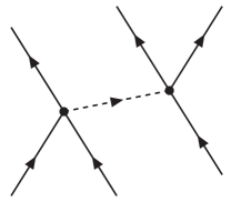
Figure 9: Three-body scattering process inducing an effective three-body coupling in low dimensions. Solid and dashed lines represent bosons in transverse ground and excited states, respectively.

Because the original three-dimensional Hamiltonian in Eq. (3.2) has a two-body coupling, the resulting Eq. (3.2) also has a two-body coupling provided by

$$g_{2}=g_{\mathrm{3D}}\int\!dydz\,[\varphi_{00}(y,z)]^{4}=\frac{2a_{\mathrm{3D}}}{ml_{\perp}^{2}}$$ (17)

to the lowest order in $a_{\mathrm{3D}}$ with $l_{\perp}=1/\sqrt{m\omega_{\perp}}$. Furthermore, Eq. (3.2) has effective three-body and higher-body couplings induced by virtual excitation of bosons to transverse excited states PhysRevLett.89.110401 ; PhysRevLett.96.030406 ; PhysRevLett.100.210403 . In particular, the three-body coupling to the lowest order in $a_{\mathrm{3D}}$ is induced by the three-body scattering process depicted in Fig. 9 and provided by

$$g_{3} =6\sum_{n=1}^{\infty}\frac{[g_{\mathrm{3D}}\int\!dydz\,\{\varphi_{00}(y,z)\}^{3}\varphi_{0n}(y,z)]^{2}}{E_{00}-E_{0n}}$$

$$=-12\ln\!\left(\frac{4}{3}\right)\frac{a_{\mathrm{3D}}^{2}}{ml_{\perp}^{2}},$$ (18)

where $\varphi_{0n}(y,z)=e^{-(\rho/l_{\perp})^{2}/2}L_{n}[(\rho/l_{\perp})^{2}]/(\sqrt{\pi}\,l_{\perp})$ with $\rho=\sqrt{y^{2}+z^{2}}$ is employed. We note that $g_{3}$ presented in Refs. PhysRevLett.96.030406 ; PhysRevLett.100.210403 was four times larger than Eq. (18) but was later corrected in Refs. PhysRevLett.105.090404 ; Mazets_2010 . Dots in Eq. (3.2) include higher-body couplings as well as couplings involving derivatives such as effective-range corrections.

The two-body coupling in Eq. (17) is linear in $a_{\mathrm{3D}}$ and can be repulsive or attractive depending on the positive or negative sign of $a_{\mathrm{3D}}$. On the other hand, the three-body coupling in Eq. (18) appears at the quadratic order in perturbation, so that it is always attractive. Because the former dominates over the latter for weakly-interacting bosons, it is generally expected that physics is essentially determined by the two-body coupling and the three-body coupling only provides quantitative corrections that may be negligible without spoiling essential physics. However, this is not the case in one dimension because the two-body and three-body couplings have distinct characters: while the two-body coupling preserves the integrability, it is broken by the three-body coupling PhysRevLett.89.110401 ; PhysRevLett.96.030406 ; PhysRevLett.100.210403 . Therefore, even if the three-body coupling is quantitatively small, it is the leading perturbation to break the integrability and may have some qualitatively significant consequences in one dimension.

In particular, because two-body scatterings in one dimension do not change the momentum distribution, it is three-body scatterings that cause thermalization of a quasi-one-dimensional Bose gas. The thermalization rate due to the effective three-body coupling was estimated in Refs. PhysRevLett.100.210403 ; Mazets_2010 and was found to be consistent with the time needed for evaporative cooling of a ⁸⁷Rb gas Hofferberth2007 ; Hofferberth2008 . Similarly, the thermal conductivity of a weakly-interacting Bose gas in quasi-one-dimension was shown to be dominated by the three-body coupling rather than the two-body coupling PhysRevE.106.064104 . Its expression was obtained as

$$\kappa=\frac{\mathcal{N}}{m^{3}g_{3}^{2}}\tilde{\kappa}\!\left(\frac{mT}{\mathcal{N}^{2}}\right),$$ (19)

where $T$ is the temperature, $\mathcal{N}$ is the number density, and $\tilde{\kappa}(*)$ is a dimensionless function determined numerically in Ref. PhysRevE.106.064104 (see Fig. 6 therein).

The three-body coupling also has significant consequences on few-body physics in one dimension. When the two-body coupling is attractive, $N$ bosons in the absence of three-body coupling are known to form a single bound state 10.1063/1.1704156 , whose binding energy is provided by

$$E_{N}^{\mathrm{(MG)}}=-\frac{N(N^{2}-1)}{24}mg_{2}^{2}.$$ (20)

Such an $N$-body cluster has no interaction (reflection probability) with an extra boson, being another manifestation of the integrability PhysRevLett.96.163201 ; PhysRevA.85.062711 . Therefore, their interaction in quasi-one-dimension is dominated by the effective three-body coupling as the leading perturbation to break the integrability. The scattering length between one boson and the $(N{-}1)$-body cluster now in the presence of three-body coupling was computed in Ref. PhysRevA.97.061603 and was found to be repulsive for $4\leq N\leq 38$ but interestingly turn attractive for $N=3$ (see also Refs. PhysRevA.97.061604 ; PhysRevA.97.061605 ) and $N\geq 39$. Because infinitesimal pairwise attraction immediately leads to a bound state in one dimension, the latter case exibits new $N$-body cluster formation induced by none other than the three-body coupling. Its binding energy measured from the dissociation threshold was predicted as

$$\Delta E_{N}^{*}=-\frac{N\beta_{1,N-1}^{2}}{8(N-1)}m^{3}g_{2}^{2}g_{3}^{2},$$ (21)

where $\beta_{1,N-1}$ is an $N$-dependent number associated with the boson-cluster scattering length PhysRevA.97.061603 (see Fig. 2 and Table I therein).

3.3 Artificial control of three-body forces

Three-body forces not only naturally appear in low dimensions, but they can also be controlled artificially with cold atoms. Accordingly, it is even possible to make three-body forces dominate over two-body forces. While several such schemes have been proposed theoretically PhysRevA.89.053619 ; PhysRevLett.112.103201 ; PhysRevA.90.021601 ; PhysRevA.93.043616 , we here introduce the simple and versatile one proposed in Ref. PhysRevA.90.021601 , which employs two hyperfine spin components of bosons in an optical lattice. When the two components are coupled by a nearly resonant field, the system in the tight-binding approximation is described by

$$\hat{H}=-t\sum_{\sigma=\uparrow,\downarrow}\sum_{\langle i,j\rangle}\hat{b}_{\sigma i}^{\dagger}\hat{b}_{\sigma j}+\sum_{i}\hat{\mathcal{H}}_{i}$$ (22)

with

$$\hat{\mathcal{H}}_{i} =-\frac{\Omega}{2}(\hat{b}_{\uparrow i}^{\dagger}\hat{b}_{\downarrow i}+\hat{b}_{\downarrow i}^{\dagger}\hat{b}_{\uparrow i})-\frac{\Delta}{2}(\hat{b}_{\uparrow i}^{\dagger}\hat{b}_{\uparrow i}-\hat{b}_{\downarrow i}^{\dagger}\hat{b}_{\downarrow i})$$

$$\quad+\sum_{\sigma,\sigma^{\prime}}\frac{u_{\sigma\sigma^{\prime}}}{2}\hat{b}_{\sigma i}^{\dagger}\hat{b}_{\sigma^{\prime}i}^{\dagger}\hat{b}_{\sigma^{\prime}i}\hat{b}_{\sigma i}.$$ (23)

Here $t$ is the inter-site tunneling amplitude, $\Omega$ is the Rabi frequency, $\Delta$ is the detuning, and $u_{\sigma\sigma^{\prime}}$ are the on-site interaction energies. Due to the Rabi coupling, the eigenstates of the spin part of Hamiltonian (first line) in Eq. (3.3) are not $\uparrow$ and $\downarrow$ bosons but their superpositions and their energies are separated by the spin gap of $\sqrt{\Omega^{2}+\Delta^{2}}$. Therefore, as far as low-energy physics relative to the spin gap is concerned, the higher-energy state cannot be excited so that bosons only occupy the lower-energy state. Accordingly, such low-energy physics of the system should be described by an effective single-component Hamiltonian in the form of

$$\hat{H}_{\mathrm{eff}}=-t\sum_{\langle i,j\rangle}\hat{b}_{i}^{\dagger}\hat{b}_{j}+\sum_{i}\sum_{n=1}^{\infty}\frac{U_{n}}{n!}\hat{b}_{i}^{\dagger n}\hat{b}_{i}^{n},$$ (24)

where $U_{n}$ is an effective $n$-body interaction energy induced by virtual excitation of bosons to the higher-energy state.

When one site is occupied by $N$ bosons, their on-site energy resulting from the second term of Eq. (24) reads

$$\sum_{n=1}^{N}\frac{N!}{n!(N-n)!}U_{n}.$$ (25)

In order for the effective Hamiltonian in Eq. (24) to be the correct low-energy description of the original Hamiltonian in Eq. (22), Eq. (25) should match the lowest on-site energy of $N$ bosons resulting from Eq. (3.3), whose matrix elements are provided by

$$\langle n|\hat{\mathcal{H}}_{i}|n^{\prime}\rangle=\begin{cases}\,\frac{N-2n}{2}\Delta+\frac{n(n-1)}{2}u_{\uparrow\uparrow}+\frac{(N-n)(N-n-1)}{2}u_{\downarrow\downarrow}\\ \quad{}+n(N-n)u_{\uparrow\downarrow}\qquad(n^{\prime}=n)\\[4.0pt] \,-\frac{\sqrt{n(N-n+1)}}{2}\Omega\qquad(n^{\prime}=n-1)\\[4.0pt] \,-\frac{\sqrt{(n+1)(N-n)}}{2}\Omega\qquad(n^{\prime}=n+1)\\[4.0pt] \ 0\qquad(\mathrm{otherwise})\end{cases}$$ (26)

with $|n\rangle=[1/\sqrt{n!(N-n)!\,}]\,\hat{b}_{\uparrow i}^{\dagger n}\,\hat{b}_{\downarrow i}^{\dagger N-n}|\mathrm{vac}\rangle$ and $n=0,1,\dots,N$. Equating its lowest eigenvalue with Eq. (25) determines $U_{N}$ for $N=1,2,\dots$ non-perturbatively as a function of $\Omega$, $\Delta$, and $u_{\sigma\sigma^{\prime}}$. Because these parameters are tunable in cold-atom experiments, independent control of $U_{N}$ is possible at least for several lowest $N$.

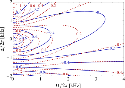
Figure 10: Contour plots of $U_{2}/2\pi$ [kHz] (blue solid curves) and $U_{3}/2\pi$ [kHz] (red dashed curves) in the $\Omega$-$\Delta$ plane. The black dot marks a point for $U_{2}=U_{3}=0$.

As a concrete application, Ref. PhysRevA.90.021601 considered ³⁹K atoms subjected to a magnetic field $\approx 58$ G in an optical lattice, where the on-site interaction energies in the harmonic approximation were estimated as $u_{\uparrow\uparrow}\approx 2\pi\times 0.55$ kHz, $u_{\downarrow\downarrow}\approx 2\pi\times 3.05$ kHz, and $u_{\uparrow\downarrow}\approx-2\pi\times 0.91$ kHz for hyperfine spin components of $F=1$, $m_{F}=-1$ ($\sigma=\ \uparrow$) and $F=1$, $m_{F}=0$ ($\sigma=\ \downarrow$) D'Errico_2007 ; PhysRevA.81.032702 . The resulting $U_{2}$ and $U_{3}$ as functions of $\Omega$ and $\Delta$ are presented in Fig. 10, where $U_{3}$ is found to be tunable in both magnitude and sign along the curve corresponding to $U_{2}=0$. In particular, $U_{2}$ and $U_{3}$ simultaneously vanish at $(\Omega,\Delta)\approx 2\pi\times(1.70,1.38)$ kHz so that $U_{4}\approx 2\pi\times 0.18$ kHz becomes the leading interaction energy PhysRevA.90.021601 . Accordingly, it is possible to realize exotic systems without two-body coupling but with a tunable three-body coupling, and even more exotic systems without two-body nor three-body couplings but with a four-body coupling in any dimensions.

Such exotic systems are expected to exhibit unique physics. Let us first consider identical bosons in two dimensions without two-body but with a three-body coupling. When the three-body attraction is tuned to a resonance where a three-body bound state just appears, four such bosons were shown to form an infinite tower of bound states with the universal scaling law of

$$E_{n}\propto e^{-2(\pi n)^{2}/27}\qquad(n\gg 1)$$ (27)

in the binding energy of $n$-th excited state PhysRevLett.118.230601 . This newly discovered few-body phenomenon is a unique consequence of the three-body coupling, which was termed the semisuper Efimov effect by analogy with the Efimov effect efimov1970energy ; efimov1973energy and the super Efimov effect PhysRevLett.110.235301 ; PhysRevA.90.063631 . This trio of effects constitutes universal classes of quantum halos whose spatial extensions can be arbitrarily large compared to the range of interaction potentials (see Sec. 4 for more details on the Efimov effect).

Turning to one dimension again, we note that a three-body coupling therein is special not only because it breaks the integrability but also because it is marginally relevant in the sense of the renormalization group if it is attractive PhysRevA.97.011602 ; PhysRevLett.120.243002 . Because the latter character is analogous to that of a two-body coupling in two dimension, similar physics is expected to emerge. In particular, Ref. PhysRevA.97.011602 showed that one-dimensional bosons without two-body but with weak three-body attraction form a many-body cluster stabilized by the quantum mechanical effect, resembling that of two-dimensional bosons PhysRevLett.93.250408 ; Bazak_2018 . Its ground-state energy normalized by that of three bosons is universal, as long as the system remains dilute, and was predicted to grow exponentially as

$$\frac{E_{N}}{E_{3}}\to\exp\!\left(\frac{8N^{2}}{\sqrt{3}\,\pi}\right)$$ (28)

with increasing number of bosons $N\gg 1$ PhysRevA.97.011602 .

Furthermore, a four-body coupling in one dimension is analogous to a two-body coupling in three dimensions in the sense that both of them are irrelevant but have a fixed point at finite attraction corresponding to a resonance where a bound state just appears PhysRevLett.101.170401 ; nishida2011liberating . As discussed in Sec. 4, three-dimensional bosons at a two-body resonance are known to exhibit the Efimov effect efimov1970energy ; efimov1973energy . Similarly, one-dimensional bosons without two-body and three-body couplings but at a four-body resonance were shown to exhibit the Efimov effect, where five such bosons form an infinite tower of bound states with the universal scaling law of

$$E_{n}\propto(12.4)^{-2n}\qquad(n\gg 1)$$ (29)

in the binding energy of $n$-th excited state PhysRevA.82.043606 . The resulting Efimov effect in one dimension is a unique consequence of the four-body coupling since the Efimov effect induced by the two-body coupling is possible only in three dimensions nielsen2001three .

Table 1: Ground-state energies of universal $N$-boson clusters for $N\gg 1$ with few-body attraction (columns) in various dimensions (rows). The (semisuper) Efimov effect indicates the universality not in the ground state but only in higher excited states. The other systems marked by dashes are considered to be non-universal.

Dim.\Att.	Two-body	Three-body	Four-body
1D	$N^{3}$ 10.1063/1.1704156	$e^{8N^{2}/\sqrt{3}\pi}$ PhysRevA.97.011602	Efimov PhysRevA.82.043606
2D	$e^{2.15N}$ PhysRevLett.93.250408	semisuper PhysRevLett.118.230601	—
3D	Efimov efimov1970energy	—	—

Our perspective developed so far on the fates of bosons with two-body, three-body, or four-body attraction in various dimensions is summarized in Table 1, which may be useful to develop further insight into the universality in quantum few-body and many-body physics.

4 Efimov physics in nuclei and atoms

4.1 Overview of the Efimov effect

Among the quantum clusters of few particles, a certain class is remarkable: those which are very close to dissociation into smaller clusters or even all the constituent particles. In quantum systems with short-range interactions, there is indeed a minimum strength of the particles’ attraction that is required for the particles to remain bound to each other. These clusters are thus realised when the attraction strength is just above such critical point, and are therefore relatively weakly bound. What is remarkable about these loosely bound clusters is that they can be very large, much larger than the range of the interactions, thanks to the ability of quantum systems to explore classically forbidden regions. One often speaks of “quantum halos” Jensen2004 when referring to these states, to emphasise their large extent and diluteness. Since a dominant part of their wave function is delocalised outside the region of interaction, it depends upon the interactions only through a few effective parameters. As a result, these states are said to be universal in the sense that only these few parameters are enough to characterise the wave function to good level of approximation, as well as many other properties such as their energy. In other words, different systems with very different interactions can nonetheless lead to the same universal states if their effective interaction parameters are the same.

Among these universal quantum halo states, a more specific class is particularly remarkable and has been a centre of attention of physicists for many years: the so-called “Efimov states”, discovered by V. Efimov in the 1970s Efimov1970a . These three-body clusters occur for inter-particle interactions that are close to the dissociation point of two particles. This means that they can exist either when their two-body subsystems themselves form loosely bound two-body halos ($1/a>0$ side of Fig. 11), or even when any of their two-body subsystems is unbound ($1/a<0$ side of Fig. 11). In the latter case, these three-body clusters are said to be “Borromean”, a fairly common property of quantum halos. But the unique feature of Efimov states is that they are bound by an effective long-range three-body force called the “Efimov attraction” arising from the short-range two-body forces between the particles. As a result of this long-range attraction, an infinite number of three-body bound states exist before any pair of particles can bind. Moreover, the Efimov attraction is scale invariant, since it decays as $1/R^{2}$, where $R$ is the size of the three-particle system. As a result, the infinity of three-body bound states near the two-body dissociation point is invariant by scaling transformations with scaling factors that are multiples of a certain number $\lambda_{0}$. This property is called “discrete scale invariance” and is depicted in Fig. 11. The figure shows in particular that the energy $E_{n}$ of the $n$th excited state at the two-body dissociation point is related to that of the next one by $E_{n}=\lambda_{0}^{2}E_{n+1}$, which gives the scaling law for the excited states:

$$E_{n}\propto\lambda_{0}^{-2n}\ \ (n\gg 1).$$ (30)

Since each three-body bound state is related to the next one by a fixed scaling transformation, it is enough to specify the energy of one particular three-body bound state to determine the energies of all other bound states. This single energy scale fixing the whole spectrum is referred to as the “three-body parameter” and is conventionally defined to be the limit of $E_{n}\lambda_{0}^{2n}$ for large $n$.

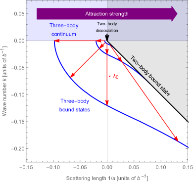
Figure 11: Efimov plot: schematic plot of three-particle energy $E$ as a function of the inverse of the scattering length $a$ between particles, which is measure of the particles’ attraction strength indicated by the wide purple arrow. The energy $E$ is rescaled into a wave number $k=\text{sign}(E)\sqrt{m|E|}/\hbar$ (where $m$ is the mass of the particles and $\hbar$ the reduced Planck constant) so that both coordinates are homogeneous to an inverse length, and can be expressed in units of the inverse of the range $b$ of the particles’ interactions. As the attraction strength is increased, the cluster of two particles (black line) appears from the point $1/a=0$ indicated by the black arrow. Conversely, this point can also be regarded as the two-body dissociation point when the attraction strength is decreased. There is an infinite number of three-particle clusters appearing before that point. Their energies form a discrete-scale invariant pattern, whereby any point on these energy curves can be mapped to another point by scaling the coordinates ($k,1/a$) by a factor $\lambda_{0}$, as indicated by the red arrows.

The occurrence of discrete-scale invariance in systems of particles with short-range interactions is called the “Efimov effect”. There are certain conditions for the Efimov effect to occur. First of all, the quantum statistics and spin of the particles play an important role, because the Pauli exclusion directly competes with the Efimov attraction efimov1973energy ; PhysRevA.67.010703 ; kartavtsev2007low ; PhysRevLett.103.153202 ; PhysRevA.86.062703 ; endo2011universal . While identical bosons are always subject to the Efimov effect whenever they are close to their two-body dissociation point, identical fermions with spin 1/2 or less (polarised fermions) cannot exhibit the Efimov effect due to the Pauli exclusion. Generally, for the Efimov effect to occur, at least two pairs of particles must be able to interact in the $s$-wave, close to their dissociation point. This means that their corresponding $s$-wave scattering lengths must be, in absolute value, much larger (typically 10 times PhysRevLett.107.120401 ; PhysRevLett.108.263001 ; pascaleno3BP1 ; pascaleno3BP2 ; johansen2017testing ; PhysRevLett.111.053202 ) than the range of their interactions. This is a rather stringent requirement, since most systems have scattering lengths of the order of the interaction range, and therefore do not exhibit the Efimov effect.

In systems where the Efimov effect occurs, the value of the scaling factor $\lambda_{0}$ depends on the quantum statistics and masses of the particles. For identical bosons, its value is $\lambda_{0}\approx 22.7$, which makes successive states very different in size and energy. For systems of particles with mass imbalance, the scaling factor can differ significantly and even approach 1 in the case of a very light particle interacting with two heavy particles efimov1973energy ; nielsen2001three ; naidon2017efimov . In this case, the energy spectrum is denser than that of identical bosons and more easily observable Pires2014 ; Tung2014 ; PhysRevLett.115.043201 .

The term “Efimov physics” naidon2017efimov has been coined to loosely designate the study of any physical situation where the Efimov effect plays a role, or an Efimov-like effect occurs. For instance, the energy spectrum of a larger number of particles, such as four bosons, may also exhibit a discrete-scale invariant pattern with the same scale factor $\lambda_{0}$ as in the three-particle spectrum, due to the influence of the 3-body Efimov effect PhysRevD.7.2517 ; hammer2007universalEPJ ; von2009signatures ; PhysRevA.70.052101 ; yamashita2006four ; PhysRevLett.107.135304 ; deltuva2011shallow ; deltuva2013properties ; PhysRevLett.108.073201 ; PhysRevLett.113.213201 . Generalisations of the Efimov effect for systems in mixed dimensions also exhibit discrete-scale invariance PhysRevLett.101.170401 ; nishida2011liberating ; PhysRevA.79.060701 ; PhysRevA.82.011605 ; PhysRevA.84.052727 . Other systems, such as particles close to dissociation in the $p$-wave, either in 3D PhysRevLett.97.023201 ; PhysRevA.86.012711 ; PhysRevA.86.012710 ; PhysRevA.77.043611 ; PhysRevLett.96.050401 ; PhysRevLett.99.210402 ; PhysRevA.106.023304 ; PhysRevA.107.033329 or 2D PhysRevLett.110.235301 ; Volosniev_2014 ; PhysRevA.92.020504 ; PhysRevA.78.063616 ; Gridnev_2014 ; PhysRevA.90.063631 , are not scale invariant but exhibit an effective long-range attraction similar to the Efimov attraction.

4.2 Geometry of Efimov states

Although the main feature of the Efimov states is the discrete scaling invariance around the two-body dissociation point, they are also characterised by universal geometric properties. For instance, at the two-body dissociation point, the three-body bound states close to zero energy (a.k.a Efimov trimers) have the same probabilistic distribution of triangular configurations, up to a global scaling by the universal factor $\lambda_{0}$. This distribution favours elongated configurations where one particle remains away from the other two. Quite counterintuitively, these typical configurations get more and more elongated as the attraction between particles gets stronger, until the three-body bound state dissociates into a two-body bound state and a free particle, as shown by the merging of the blue curves with the black curve in Fig. 11. On the opposite side (Borromean region), where the attraction between particles is weaker, the configurations become more equilateral. Interestingly, near the three-body dissociation, they conform to another universal pattern known as “halo universality” Fedorov1994a ; Jensen2004 ; naidon2023universal . Halo universality is a generic feature of few-body systems close to their full dissociation threshold and is independent of the Efimov effect itself. Unlike Efimov universality, which is characterised by a scaling factor between consecutive states (and thus difficult to demonstrate), halo universality is characterised by a universal geometry: all distances in the three-body system diverge when the binding energy approaches zero, thereby turning the system into a halo, but their ratios have well defined values. Remarkably, this universal halo geometry generally applies to states close to their three-body dissociation point, including the ground state, in sharp contrast with the Efimov universality which is accurate only for excited states.

In the case of three identical bosons, the universal halo geometry close to the three-body threshold is characterised by an equiprobability of all the triangular configurations of the three bosons. In the case of two identical particles and another particle, the universal halo geometry depends on the scattering length $a\gg b$ between the two identical particles and the binding energy $\kappa=\sqrt{m|E|}/\hbar\ll b$ of the system: when $\kappa a\ll 1$, it is the same universal halo geometry as that of three bosons, but when $\kappa a\gg 1$ it goes to a different geometry. These universal geometric properties can be derived analytically as a function of $\kappa a$ PhysRevLett.128.212501 ; naidon2023universal .

4.3 Efimov states in nuclear physics

The major requirement for the conventional Efimov effect to occur is having pairs of particles with scattering lengths much larger than the range of their interactions. It turns out that the scattering lengths for nucleons are relatively large, with both the triplet scattering length $a_{t}\approx 5$ fm and the singlet scattering length $a_{s}\approx-20$ fm being larger than the range of nuclear forces, which is of the order of 1 fm. However, the Coulomb repulsion between protons, which is a long-range force and introduces an additional scale, can easily spoil the Efimov effect; for example, the Hoyle state hoyle1954nuclear ; efimov1970energy , the excited state of ¹²C nuclei, argued to be analogous to the Efimov state of three $\alpha$ particles, is significantly affected by the Coulomb interaction and cannot be described by the universal Efimov theory hammer2008model ; PhysRevC.91.014004 ; otsuka2022alpha . Therefore, the Efimov states investigated so far in nuclear physics mostly involve two neutrons interacting with a nucleus.

Triton.

The simplest example is the triton, the system composed of two neutrons and one proton efimov1970energy ; naidon2017efimov . This system fits qualitatively into the Efimov plot of Fig. 11, but for a positive scattering length $a=a_{t}$ that is not so large compared to the interaction range $b$, thus on the right-hand side of Fig. 11 where only one three-body bound state exists. Indeed, there is no excited bound state of the triton. It is thus impossible to check the discrete-scale invariance, which is a hallmark of the Efimov effect. Yet, the universal features of the Efimov effect can readily explain some theoretical properties of the triton, such as the Phillips line phillips1968consistency ; efimov1985explanation ; efimov1988correlation , which is a correlation between the triton energy and the neutron-deuteron spin-doublet scattering length.

Halo nuclei.

Systems of two neutrons interacting with a nucleus are more promising candidates for Efimov states. Although a single neutron tends to be absorbed by a nucleus due to the strong force, the situation changes when the number of neutrons becomes large and approaches the neutron dripline where neutrons is no longer tighty bound around the nucleus. Around this dripline, it may happen for certain nuclides that they could almost but not quite bind an extra neutron. If one regards the nucleus and the neutron as two distinct particles, this situation corresponds to the two-body dissociation point discussed earlier, around which the Efimov effect can occur. It is thus expected that, in the presence of two neutrons, such a nucleus could form a three-body Efimov state, where the two neutrons would remain at large distance forming a halo around the nucleus. Indeed, nuclei with two-neutron halo structures have been studied both experimentally and theoretically since the 1980s, such as ⁶He, ¹¹Li, ¹²Be, ¹⁷B, ¹⁹B, ²⁰C, ²²C, ⁶²Ca, and ⁷²Ca tanihata1985measurements ; AlKhalili2004 ; Tanihata2013 ; Fedorov1994 ; Amorim1997 ; AnnRev_HamPlatt ; naidon2017efimov ; FREDERICO2012939 ; Canham2008 ; Hammer_2017 ; ACHARYA2013196 ; PhysRevLett.111.132501 ; PhysRevC.105.024310 ; PhysRevLett.120.052502 . Compared to the triton, these systems stand as better candidates for Efimov states Fedorov1994 ; Amorim1997 ; Canham2008 because some of them would correspond to the Borromean regime (left-hand side of Fig. 11) where the universal description in terms of Efimov state is more effective. It is indeed widely believed that these two-neutron halo nuclei are examples of Efimov states. Three-body models of some nuclei seem to reproduce observations and confirm this view.

However, the Efimov scenario as shown in Fig. 11 is difficult to evidence in two-neutron halo nuclei because of several factors. First, the $s$-wave scattering length between the core nucleus and a neutron may not be large enough. Typical values for the neutron-rich nuclei are 5-10 fm. This limits the number of Efimov states as $\dfrac{1}{\pi}\mathrm{ln}\left(\frac{|a|}{b}\right)\lesssim 1$, which precludes the possibility of observing two adjacent trimers and testing the discrete scale invariance. As the synthesis of the neutron-rich nuclei is currently limited to light nuclei, the good candidates to see the excited Efimov state with current experimental techniques are likely be ¹⁹B and ²²C. In particular, a large $s$-wave scattering length is reported in ¹⁷B-n as $\gtrsim 100$ fm SPYROU2010129 ; carbonell2020low ; PhysRevLett.121.262502 , which may currently be the best candidate to see the elusive excited Efimov state in neutron-rich nuclei PhysRevC.100.011603 . Second, the size of the trimer is not large enough and the core may not be regarded as a featureless inert point particle. Rather, the size and internal structure of the core nucleus may play a significant role. In such cases, the collective excitations of the core may couple with the halo neutrons. The halo neutrons may also have significant correlations with the neutrons inside the core nucleus, in which case the two neutrons are better described as forming a BCS-like pair induced by the Fermi sea of the nuclei, rather than the three-body Efimov picture. Even when the three-body picture is valid, contributions from higher partial waves may play a significant role, as in ⁶He, ¹¹Li PhysRevC.50.R550 ; PhysRevC.90.044004 . Finally, the effective range (i.e. finite radius of the nucleus) may not be negligible, so that finite-range corrections to the zero-range universal Efimov theory must be taken into account. Further experimental observations and comparison with three-body models are thus necessary to confirm whether two-neutron halo nuclei do indeed conform to the geometry of Efimov states.

Interestingly, the geometry of Efimov states near three-body dissociation tends to the universal halo geometry mentioned in Sec. 4.2. Thus, if two-neutron halo nuclei are indeed Borromean Efimov states, they should approach this halo universality. However, the neutron-neutron scattering length is somewhat too small with respect to $b$ to fully reach the universal halo regime, so that they only constitute approximations of such halos. Among the known two-neutron halo nuclei, ¹⁹B and ²²C are good candidates to exhibit the halo universality naidon2023universal . This could be experimentally confirmed by improving the measurements of their various mean square radii and binding energies.

Excited nuclei.

Recently, stable nuclei excited around their neutron breakup thresholds have been proposed as novel nuclear candidates exhibiting an enormous $s$-wave scattering length and the Efimov states endotanaka2023 . While the stable nuclei well inside the valley of stability of the nuclear chart do not show any halo structure in their ground states, they may form an $s$-wave halo of a core nucleus and a neutron if they are excited in the vicinity of the one-neutron separation threshold, around which the neutron may be barely bound by the core nucleus. From the thermal neutron capture cross section data shusterman2019surprisingly , it has been argued that ${}^{88}\mathrm{Zr}$ and ${}^{157}\mathrm{Gd}$ should have very large $s$-wave halo, and hence large $s$-wave scattering lengths $|a|\gtrsim 10^{4}$ fm, which is 1-2 orders of magnitude larger than those in the neutron-rich nuclei. It is predicted that there are at least one and possibly two Efimov trimers made of the core plus two neutrons in ${}^{90}\mathrm{Zr}$ and ${}^{159}\mathrm{Gd}$, which appear as sub-threshold excited state around the two-neutron separation threshold. It has also been conjectured that the $s$-wave halo and the Efimov states may universally appear in the stripe regions of the nuclear chart when the new excitation energy axis is added above the nuclear chart, presenting a global picture to encompass the Efimov physics in the neutron-rich nuclei and the Efimov physics in the excited nuclei around the neutron separation threshold. This new perspective needs to be confirmed by further theoretical and experimental studies.

4.4 Efimov states in atomic physics

4.4.1 Helium-4

Atomic physics has been more favourable for the demonstration of the Efimov effect. Soon after its prediction, it was realised that helium-4 atoms are good candidates for the observation of Efimov states, since they are bosonic and their $s$-wave scattering length happens to be about 20 times larger than their interaction range. This allows the existence of two trimer states, a ground state and an excited state Lim1977 . There was a long experimental effort to observe these states, which involved diffracting beams of helium clusters through a grating, selecting the deflecting beam corresponding to trimers and analysing their geometry. Although the ground state was observed from the 1990s Schoellkopf1994 ; Bruehl2005 , it does not fully conform to the Efimov zero-range theory. Observation of the excited state was finally reported in 2015 Kunitski2015 , thanks to the Coulomb explosion imaging technique. It revealed that its geometry excellently conform to the Efimov theory, although the universal scaling ratio $\lambda_{0}$ could not be directly confirmed.

4.4.2 Cold atoms

Although helium-4 was for a long time the only candidate for the observation of Efimov states, it turned out that the atomic species used in cold-atom experiments are even better for this purpose. Although their natural scattering lengths are usually not large enough to expect the existence of Efimov states in these atomic systems, it is possible to alter the scattering length at will by applying a magnetic field onto these atoms, thanks to the so-called magnetic Feshbach resonances Tiesinga1993 ; Chin2010 . This allows to experimentally probe the Efimov plot of Fig. 11, not only at a single scattering length value as in the case of helium-4 or halo nuclei, but over a whole range of scattering lengths.

Observing Efimov states via three-body loss.

The simplest way to reveal the presence of Efimov states in this range is to monitor the losses occurring among atoms through three-body collisions and recombinations into deeply bound dimers PhysRevLett.83.1751 ; PhysRevLett.85.908 . Indeed, nearby the scattering lengths at which an Efimov state appears at the three-body zero-energy threshold, these losses are significantly enhanced by the three-body resonances above threshold associated to these Efimov states Kraemer2006 ; PhysRevLett.103.163202 ; zaccanti2009observation ; pollack2009universality . Since these scattering lengths are related to each other by a scaling with the universal scaling ratio $\lambda_{0}$, it makes possible the experimental determination of this ratio. The discrete scale invariance was thus confirmed in both systems of identical bosons Huang2014 and systems of heavy bosons interacting with a lighter boson Tung2014 ; Pires2014 . The measured scaling ratios were found to be consistent with the universal predictions, within the experimental uncertainties and corrections due to the finite-range of interactions. To minimize the effects of finite temperatures, trap size, and other aspects deteriorating Efimov signatures, there is an on-going attempt to observe Efimov states in the microgravity environment aboard the International Space Station (ISS) elliott2018nasa ; oudrhiri2023nasa ; frye2021bose .

Direct association of Efimov states.

In addition to observing the Efimov states through losses, there has also been efforts to directly probe the Efimov states LompeScience11 ; PhysRevLett.106.143201 ; PhysRevLett.108.210406 . This can be done by shining a radio-frequency (RF) pulse to a mixture of atoms and Feshbach dimers. The atoms are initially prepared in a hyperfine state $|0\rangle$, while the dimers composed of two atoms in the $|1\rangle$ and $|2\rangle$ hyperfine states. A certain frequency of the RF pulse can drive the atoms in hyperfine state $|0\rangle$ to a hyperfine state $|3\rangle$. If that state has a simultaneous Feshbach resonant interaction with the atoms remaining in states $|1\rangle$ and $|2\rangle$, there are Efimov states composed of atoms in $|1\rangle$, $|2\rangle$, and $|3\rangle$ states just below this threshold. It is thus possible to form these Efimov states from the initial mixture by shining a slightly reduced RF frequency. By measuring the frequency difference, one can directly obtain the binding energies of the trimers. Such a system can be prepared with ⁶Li atoms, for which there is a magnetic field region where the $s$-wave scattering length between the three hyperfine states can be simultaneously large. In Refs. LompeScience11 ; PhysRevLett.106.143201 , such a direct photo-association of an Efimov trimer has been performed, and its binding energy has been directly measured. This RF association can also be performed without the Feshbach dimer; in Ref. PhysRevLett.108.210406 , the RF association of an Efimov trimer has been successfully performed with ⁷Li atoms from an initial state where all atoms are unbound. This method, while not requiring three resonant hyperfine states nor Feshbach dimers, relies on a large spatial overlap between the initial three-atom state and the final Efimov state and therefore can only be performed around the dissociation point of the Efimov trimer. More recently, Efimov trimers have also been created from a low-temperature Bose-Einstein condensate of atoms by rapidly sweeping a magnetic field, hence varying the $s$-wave scattering length from small positive values to large positive values for which Efimov trimers exist PhysRevLett.119.143401 .

Coherent association of Efimov states.

While the above methods can directly create and probe Efimov trimers, the associated trimers undergo a three-body recombination and soon get lost from the trap. Recently, the group of Lev Khaykovich has observed coherent signatures of Efimov trimers in a manner insensitive to their recombination loss PhysRevLett.122.200402 ; yudkin2023reshape ; they initially prepare cold ⁷Li atoms on the positive $a>0$ side of the Feshbach resonance, and shine a short RF pulse which is tuned to induce a transition into a superposition of an Efimov trimer state and a Feshbach dimer + atom state. The superposition state undergoes a time evolution with a phase factor which differs by $E_{t}-E_{d}$ where $E_{t}$ and $E_{d}$ are the energies of the Efimov trimer and Feshbach dimer. After a hold time $T$, the second short RF pulse turns the states back into the initial three-atom states. The final atom number count shows an oscillation $\cos[(E_{t}-E_{d})T]$ from which the binding energy of the Efimov trimer relative to the dimer energy can be obtained PhysRevLett.122.200402 . The oscillation is coherent and insensitive to the loss of Efimov states as long as the hold time $T$ is smaller than the lifetime of the Efimov states. With this technique, the binding energy of an Efimov trimer can be measured as a function of the $s$-wave scattering length yudkin2023reshape . While this technique has the advantage of enabling coherent control of the Efimov trimer, currently it can only access the $a>0$ region in the vicinity of the dimer+atom breakup threshold of the Efimov state, because the width of the RF pulse must cover both the Efimov state and the dimer+atom state to create their superposition.

Fermionic Efimov states.

While the Efimov states for bosonic atoms have been successfully observed for various atomic species, there have been ongoing efforts to observe the Efimov states with fermions. For the fermionic ⁶Li atoms, the Efimov states have been observed for atoms in three different hyperfine states PhysRevLett.103.130404 ; PhysRevA.80.040702 ; PhysRevLett.106.143201 ; PhysRevLett.108.210406 . Three atoms in different internal states can be regarded as distinguishable particles, so that the Pauli exclusion principle does not play any role and the properties of the Efimov states are essentially the same as those for bosons. In order to realize Efimov states affected by the Pauli exclusion principle, one needs to prepare fermionic atoms in the same hyperfine state. Since a resonantly large $s$-wave interaction is necessary, the simplest setup is a system of two fermionic atoms in the same hyperfine state interacting with another distinguishable atom via a large $s$-wave scattering length. According to the theoretical arguments efimov1973energy ; PhysRevA.67.010703 ; kartavtsev2007low ; PhysRevLett.103.153202 ; PhysRevA.86.062703 ; endo2011universal , such a system can form Efimov trimers if the mass ratio is above the critical value of $13.6$. Notably, the predicted Efimov trimers of fermions are characterized by a total orbital angular momentum of $\ell=1$, which is a new feature compared with the bosonic Efimov states with $\ell=0$. Therefore, they are expected to manifest different universal properties than the bosonic ones zhao2023effects ; SciPostPhys.12.6.185 ; OiEndo2024

To realize such a cold-atom system with a large mass ratio, we need a fermionic atomic species with a large enough mass. A mixture of fermionic Yb and Li atoms has been successfully cooled down to their Fermi degeneracy PhysRevLett.106.205304 . While the mass ratio is large enough to support the Efimov states, Yb-Li mixture is found to have no useful magnetic Feshbach resonances in an easily accessible range of the experiments PhysRevLett.108.043201 ; chen2015anisotropy ; PhysRevX.10.031037 ; PhysRevA.96.032711 , owing to closed-shell electronic structure of Yb atom.

More recently, an ultracold mixture of Er and Li atoms has been realized PhysRevA.107.L031306 . The Er and Li atoms are cooled down by a sympathetic cooling method utilizing the Yb atoms as a coolant, which is so powerful that a new kind of quantum degenerate gases of dual BECs of highly-magnetic atoms of Er and totally-nonmagnetic atoms of Yb can also successfully be created. The Er-Li system (mass ratio $\approx 28$) is deemed as a major candidate to realize the fermionic Efimov states. As both Er and Li atoms have open-shell atomic structures, they may have magnetic Feshbach resonances broad enough to accurately control the scattering length PhysRevA.92.022708 . Recently, systematic measurements of Er-Li Feshbach resonances for various isotope mixtures have been performed in a magnetic field range below 1 kG, and succeeded in observing many Feshbach resonances schafer_feshbach_2022 ; 167Er6Li2023 . While the observed Feshbach resonances are mostly narrow, possibly induced by the anisotropic electrostatic interactions or dipolar interactions chen2015anisotropy , several broad Feshbach resonances were also found

The observed broad Feshbach resonances in Er-Li is an important step toward observing the fermionic Efimov trimers. The Efimov trimers are expected to be observed from the loss measurement. In particular, the loss process involving the Er-Er-Li channel, namely two Er accompanied by one Li atoms should be predominantly enhanced. In Ref 167Er6Li2023 , the atom loss behavior around the Feshbach resonance at $455$ G is observed in detail for the ¹⁶⁷Er and ⁶Li mixture. The atom loss is found to be predominantly induced through the Er-Er-Li channel, namely two Er accompanied by one Li, which is consistent with the formation of the fermionic Efimov trimers. It is also shown that the shape of the observed resonance is asymmetric, which is also consistent with the previous observations of multiple losses originated from the formation of several Efimov trimers Pires2014 ; Tung2014 . More detailed measurements, including the determination of the inter-species scattering lengths, will reveal the behaviors of these resonant losses induced by the fermionic Efimov trimers in this mass-imbalanced Er-Li mixture. Due to the strong magnetic dipole interaction between Er atoms, an interplay of the van der Waals and dipole interaction is predicted to lead to novel universal behaviors of the Efimov states OiEndo2024 . We also note that the Er-Li mixture is also a fascinating candidate for realizing a novel $p$-wave superfluid of fermions of Er through the induced attraction via a BEC of light Li atoms PhysRevA.61.053601 ; PhysRevLett.117.245302 ; gurarie2007resonantly ; yamaguchi2017novel , which is also interesting from the viewpoint of the effect of the many-body background of the novel Efimov trimers.

5 Summary

We have reviewed three-body forces and related phenomena from an interdisciplinary perspective across nuclei and atoms. The three-body forces have been a key element in accurate accounts of nuclear properties, and we have reviewed recent theoretical and experimental progress on the nuclear three-body forces. We have also reviewed some recent attempts to observe, control, and quantum-simulate three-body and higher-body forces in cold atoms. We have also shown how the Efimov states appear universally across nuclear and atomic systems, and overviewed the recent developments in their observation and understanding. The three-body forces and three-body phenomena have thus been an active area of research, not only as a specific field of research or methodology, but involving various disciplines of physics and scales. With further developments in experimental technologies and theoretical methods, it is expected that three-body forces will be determined with ever more accuracy, and new quantum phenomena will be uncovered by further exploring the implications of three-body physics.

- (1) H.W. Hammer, A. Nogga, A. Schwenk, Rev. Mod. Phys. 85, 197 (2013)
- (2) J. Fujita, H. Miyazawa, Progress of Theoretical Physics 17(3), 360 (1957)
- (3) H. Yukawa, Proc. Phys. Math. Soc. Japan 17, 48 (1935)
- (4) S. Coon, H. Han, Few-Body Syst. 30, 131 (2001)
- (5) B.S. Pudliner, V.R. Pandharipande, J. Carlson, S.C. Pieper, R.B. Wiringa, Phys. Rev. C 56, 1720 (1997)
- (6) S. Weinberg, Phys. Lett. B 251, 288 (1990)
- (7) U. van Kolck, Phys. Rev. C 49, 2932 (1994)
- (8) E. Epelbaum, A. Nogga, W. Glöckle, H. Kamada, U.G. Meißner, H. Witala, Phys. Rev. C 66, 064001 (2002)
- (9) C.R. Chen, G.L. Payne, J.L. Friar, B.F. Gibson, Phys. Rev. C 33, 1740 (1986)
- (10) T. Sasakawa, S. Ishikawa, Few-Body Syst. 1(1), 3 (1986)
- (11) R.B. Wiringa, V.G.J. Stoks, R. Schiavilla, Phys. Rev. C 51, 38 (1995)
- (12) R. Machleidt, Phys. Rev. C 63, 024001 (2001)
- (13) V.G.J. Stoks, R.A.M. Klomp, C.P.F. Terheggen, J.J. de Swart, Phys. Rev. C 49, 2950 (1994)
- (14) A. Nogga, H. Kamada, W. Glöckle, B.R. Barrett, Phys. Rev. C 65, 054003 (2002)
- (15) S.C. Pieper, K. Varga, R.B. Wiringa, Phys. Rev. C 66, 044310 (2002)
- (16) M. Piarulli, et al., Phys. Rev. Lett. 120(5), 052503 (2018)
- (17) P. Navrátil, W.E. Ormand, Phys. Rev. C 68, 034305 (2003)
- (18) G. Hagen, M. Hjorth-Jensen, G.R. Jansen, R. Machleidt, T. Papenbrock, Phys. Rev. Lett. 108, 242501 (2012)
- (19) A. Cipollone, C. Barbieri, P. Navrátil, Phys. Rev. C 92(1), 014306 (2015)
- (20) T.A. Lähde, U.G. Meißner, Nuclear Lattice Effective Field Theory: An introduction (Springer, 2019)
- (21) A. Akmal, V.R. Pandharipande, D.G. Ravenhall, Phys. Rev. C 58, 1804 (1998)
- (22) S. Gandolfi, J. Carlson, S. Reddy, A.W. Steiner, R.B. Wiringa, Eur. Phys. J. A 50, 10 (2014)
- (23) J.E. Lynn, I. Tews, J. Carlson, S. Gandolfi, A. Gezerlis, K.E. Schmidt, A. Schwenk, Phys. Rev. Lett. 116, 062501 (2016)
- (24) E. Epelbaum, H.W. Hammer, U.G. Meißner, Rev. Mod. Phys. 81, 1773 (2009)
- (25) N. Kalantar-Nayestanaki, E. Epelbaum, J.G. Messchendorp, A. Nogga, Rep. Prog. Phys. 75(1), 016301 (2011)
- (26) K. Hebeler, Phys. Rep. 890, 1 (2021)
- (27) J. Haidenbauer, U.G. Meißner, N. Kaiser, W. Weise, Eur. Phys. J. A 53(6), 121 (2017)
- (28) S. Weinberg, Physica A 96(1-2), 327 (1979)
- (29) J. Gasser, H. Leutwyler, Ann. Phys. 158, 142 (1984)
- (30) S. Weinberg, Phys. Rev. 166, 1568 (1968)
- (31) S.R. Coleman, J. Wess, B. Zumino, Phys. Rev. 177, 2239 (1969)
- (32) C.G. Callan, Jr., S.R. Coleman, J. Wess, B. Zumino, Phys. Rev. 177, 2247 (1969)
- (33) V. Bernard, N. Kaiser, U.G. Meißner, Int. J. Mod. Phys. E 4, 193 (1995)
- (34) N. Fettes, U.G. Meißner, S. Steininger, Nucl. Phys. A 640, 199 (1998)
- (35) N. Fettes, U.G. Meißner, M. Mojzis, S. Steininger, Ann. Phys. 283, 273 (2000). [Erratum: Annals Phys. 288, 249–250 (2001)]
- (36) E.E. Jenkins, A.V. Manohar, Phys. Lett. B 255, 558 (1991)
- (37) V. Bernard, N. Kaiser, J. Kambor, U.G. Meißner, Nucl. Phys. B 388, 315 (1992)
- (38) T. Becher, H. Leutwyler, Eur. Phys. J. C 9, 643 (1999)
- (39) J. Gegelia, G. Japaridze, Phys. Rev. D 60, 114038 (1999)
- (40) T. Fuchs, J. Gegelia, G. Japaridze, S. Scherer, Phys. Rev. D 68, 056005 (2003)
- (41) S. Weinberg, Nucl. Phys. B 363, 3 (1991)
- (42) C. Ordonez, L. Ray, U. van Kolck, Phys. Rev. C 53, 2086 (1996)
- (43) S. Pastore, R. Schiavilla, J.L. Goity, Phys. Rev. C 78, 064002 (2008)
- (44) S. Pastore, L. Girlanda, R. Schiavilla, M. Viviani, R.B. Wiringa, Phys. Rev. C 80, 034004 (2009)
- (45) S. Pastore, L. Girlanda, R. Schiavilla, M. Viviani, Phys. Rev. C 84, 024001 (2011)
- (46) A. Baroni, L. Girlanda, S. Pastore, R. Schiavilla, M. Viviani, Phys. Rev. C 93(1), 015501 (2016). [Erratum: Phys.Rev.C 93, 049902 (2016), Erratum: Phys.Rev.C 95, 059901 (2017)]
- (47) E. Epelbaum, W. Glöckle, U.G. Meißner, Nucl. Phys. A 637, 107 (1998)
- (48) E. Epelbaum, W. Glöckle, U.G. Meißner, Nucl. Phys. A 671, 295 (2000)
- (49) E. Epelbaum, U.G. Meißner, W. Glöckle, Nucl. Phys. A 714, 535 (2003)
- (50) E. Epelbaum, U.G. Meißner, Phys. Rev. C 72, 044001 (2005)
- (51) E. Epelbaum, Phys. Lett. B 639, 456 (2006)
- (52) E. Epelbaum, Eur. Phys. J. A 34, 197 (2007)
- (53) V. Bernard, E. Epelbaum, H. Krebs, U.G. Meißner, Phys. Rev. C 77, 064004 (2008)
- (54) V. Bernard, E. Epelbaum, H. Krebs, U.G. Meißner, Phys. Rev. C 84, 054001 (2011)
- (55) H. Krebs, A. Gasparyan, E. Epelbaum, Phys. Rev. C 85, 054006 (2012)
- (56) H. Krebs, A. Gasparyan, E. Epelbaum, Phys. Rev. C 87(5), 054007 (2013)
- (57) S. Kolling, E. Epelbaum, H. Krebs, U.G. Meißner, Phys. Rev. C 80, 045502 (2009)
- (58) Kolling, S. and Epelbaum, E. and Krebs, H. and Meißner, U.-G., Phys. Rev. C 84, 054008 (2011)
- (59) H. Krebs, E. Epelbaum, U.G. Meißner, Ann. Phys. 378, 317 (2017)
- (60) H. Krebs, E. Epelbaum, U.G. Meißner, Few-Body Syst. 60(2), 31 (2019)
- (61) H. Krebs, E. Epelbaum, U.G. Meißner, Eur. Phys. J. A 56(9), 240 (2020)
- (62) N. Kaiser, R. Brockmann, W. Weise, Nucl. Phys. A 625, 758 (1997)
- (63) N. Kaiser, S. Gerstendorfer, W. Weise, Nucl. Phys. A 637, 395 (1998)
- (64) N. Kaiser, Phys. Rev. C 61, 014003 (2000)
- (65) N. Kaiser, Phys. Rev. C 62, 024001 (2000)
- (66) N. Kaiser, Phys. Rev. C 63, 044010 (2001)
- (67) N. Kaiser, Phys. Rev. C 64, 057001 (2001)
- (68) N. Kaiser, Phys. Rev. C 65, 017001 (2002)
- (69) D.R. Entem, N. Kaiser, R. Machleidt, Y. Nosyk, Phys. Rev. C 92(6), 064001 (2015)
- (70) E. Epelbaum, Prog. Part. Nucl. Phys. 57, 654 (2006)
- (71) R. Machleidt, D.R. Entem, Phys. Rep. 503, 1 (2011)
- (72) E. Epelbaum, H. Krebs, P. Reinert, Front. Phys. 8, 98 (2020)
- (73) H. Krebs, Eur. Phys. J. A 56(9), 234 (2020)
- (74) J. de Vries, E. Epelbaum, L. Girlanda, A. Gnech, E. Mereghetti, M. Viviani, Front. Phys. 8, 218 (2020)
- (75) G.P. Lepage, Lecture note of 8th Jorge Andre Swieca Summer School on Nuclear Physics pp. 135–180 (1997)
- (76) A.M. Gasparyan, E. Epelbaum, Phys. Rev. C 105(2), 024001 (2022)
- (77) A.M. Gasparyan, E. Epelbaum, Phys. Rev. C 107(4), 044002 (2023)
- (78) F. Gross, et al., Eur. Phy. J. C 83(12), 1125 (2023)
- (79) E. Epelbaum, W. Glöckle, U.G. Meißner, Nucl. Phys. A 747, 362 (2005)
- (80) D.R. Entem, R. Machleidt, Phys. Rev. C 68, 041001 (2003)
- (81) E. Epelbaum, H. Krebs, U.G. Meißner, Eur. Phys. J. A 51(5), 53 (2015)
- (82) E. Epelbaum, H. Krebs, U.G. Meißner, Phys. Rev. Lett. 115(12), 122301 (2015)
- (83) P. Reinert, H. Krebs, E. Epelbaum, Eur. Phys. J. A 54(5), 86 (2018)
- (84) R. Navarro Pérez, J.E. Amaro, E. Ruiz Arriola, Phys. Rev. C 88, 024002 (2013). [Erratum: Phys.Rev.C 88, 069902 (2013)]
- (85) P. Reinert, H. Krebs, E. Epelbaum, Phys. Rev. Lett. 126(9), 092501 (2021)
- (86) E. Epelbaum, H. Krebs, P. Reinert, Handbook of Nuclear Physics pp. 1–25 (2022)
- (87) E. Epelbaum, et al., Eur. Phys. J. A 56(3), 92 (2020)
- (88) G.F. Cox, G.H. Eaton, C.P. Van Zyl, O.N. Jarvis, B. Rose, Nucl. Phys. B 4, 353 (1968)
- (89) O.N. Jarvis, C. Whitehead, M. Shah, Phys. Lett. B 36(4), 409 (1971)
- (90) A. Taylor, E. Wood, L. Bird, Nuclear Physics 16(2), 320 (1960)
- (91) V.G.J. Stoks, R.A.M. Klomp, M.C.M. Rentmeester, J.J. de Swart, Phys. Rev. C 48, 792 (1993)
- (92) M.C.M. Rentmeester, R.G.E. Timmermans, J.L. Friar, J.J. de Swart, Phys. Rev. Lett. 82, 4992 (1999)
- (93) M.C. Birse, J.A. McGovern, Phys. Rev. C 70, 054002 (2004)
- (94) D.R. Entem, R. Machleidt, Y. Nosyk, Phys. Rev. C 96(2), 024004 (2017)
- (95) M. Piarulli, L. Girlanda, R. Schiavilla, R. Navarro Pérez, J.E. Amaro, E. Ruiz Arriola, Phys. Rev. C 91(2), 024003 (2015)
- (96) R. Somasundaram, J.E. Lynn, L. Huth, A. Schwenk, I. Tews, Phys. Rev. C 109, 034005 (2024)
- (97) S.K. Saha, D.R. Entem, R. Machleidt, Y. Nosyk, Phys. Rev. C 107(3), 034002 (2023)
- (98) D.R. Phillips, C. Schat, Phys. Rev. C 88(3), 034002 (2013)
- (99) E. Epelbaum, A.M. Gasparyan, H. Krebs, C. Schat, Eur. Phys. J. A 51(3), 26 (2015)
- (100) K. Topolnicki, Eur. Phys. J. A 53(9), 181 (2017)
- (101) S. Weinberg, Phys. Lett. B 295, 114 (1992)
- (102) S. Ishikawa, M.R. Robilotta, Phys. Rev. C 76, 014006 (2007)
- (103) L. Girlanda, A. Kievsky, L.E. Marcucci, M. Viviani, Phys. Rev. C 102, 064003 (2020)
- (104) L. Girlanda, E. Filandri, A. Kievsky, L.E. Marcucci, M. Viviani, Phys. Rev. C 107(6), L061001 (2023)
- (105) L. Girlanda, A. Kievsky, M. Viviani, Phys. Rev. C 84(1), 014001 (2011). [Erratum: Phys.Rev.C 102, 019903 (2020)]
- (106) E. Epelbaum, U.G. Meißner, J.E. Palomar, Phys. Rev. C 71, 024001 (2005)
- (107) J.L. Friar, U. van Kolck, M.C.M. Rentmeester, R.G.E. Timmermans, Phys. Rev. C 70, 044001 (2004)
- (108) S.N. Yang, Phys. Rev. C 19, 1114 (1979)
- (109) S.N. Yang, J. Phys. G 9, L115 (1983)
- (110) D. Siemens, V. Bernard, E. Epelbaum, A. Gasparyan, H. Krebs, U.G. Meißner, Phys. Rev. C 94(1), 014620 (2016)
- (111) D. Siemens, J. Ruiz de Elvira, E. Epelbaum, M. Hoferichter, H. Krebs, B. Kubis, U.G. Meißner, Phys. Lett. B 770, 27 (2017)
- (112) M. Hoferichter, J. Ruiz de Elvira, B. Kubis, U.G. Meißner, Phys. Rev. Lett. 115(19), 192301 (2015)
- (113) V. Bernard, N. Kaiser, U.G. Meißner, Nucl. Phys. A 615, 483 (1997)
- (114) T.R. Hemmert, B.R. Holstein, J. Kambor, J. Phys. G 24, 1831 (1998)
- (115) V. Pascalutsa, D.R. Phillips, Phys. Rev. C 67, 055202 (2003)
- (116) D.L. Yao, D. Siemens, V. Bernard, E. Epelbaum, A.M. Gasparyan, J. Gegelia, H. Krebs, U.G. Meißner, JHEP 05, 038 (2016)
- (117) A.N. Hiller Blin, T. Ledwig, M.J. Vicente Vacas, Phys. Lett. B 747, 217 (2015)
- (118) M. Thürmann, E. Epelbaum, A.M. Gasparyan, H. Krebs, Phys. Rev. C 103(3), 035201 (2021)
- (119) H. Krebs, E. Epelbaum, U.G. Meißner, Eur. Phys. J. A 32, 127 (2007)
- (120) E. Epelbaum, H. Krebs, U.G. Meißner, Phys. Rev. C 77, 034006 (2008)
- (121) E. Epelbaum, H. Krebs, U.G. Meißner, Nucl. Phys. A 806, 65 (2008)
- (122) H. Krebs, A.M. Gasparyan, E. Epelbaum, Phys. Rev. C 98(1), 014003 (2018)
- (123) E. Epelbaum, Proceedings of 6th International Conference Nuclear Theory in Supercomputing Era (2019)
- (124) H. Krebs, PoS CD2018, 031 (2019)
- (125) M. Luscher, P. Weisz, JHEP 02, 051 (2011)
- (126) M. Luscher, JHEP 04, 123 (2013)
- (127) M. Lüscher, PoS LATTICE2013, 016 (2014)
- (128) H. Krebs, E. Epelbaum, arXiv preprint arXiv:2312.13932 (2023)
- (129) H. Krebs, E. Epelbaum, arXiv preprint arXiv:2311.10893 (2023)
- (130) W. Glöckle, H. Witała, D. Huber, H. Kamada, J. Golak, Phys. Rep. 274, 107 (1996)
- (131) H. Witała, J. Golak, W. Glöckle, H. Kamada, Phys. Rev. C 71, 054001 (2005)
- (132) H. Witała, J. Golak, R. Skibiński, W. Glöckle, H. Kamada, W.N. Polyzou, Phys. Rev. C 83, 044001 (2011). [Erratum: Phys.Rev.C 88, 069904 (2013)]
- (133) E. Epelbaum, U.G. Meißner, Ann. Rev. Nucl. Part. Sci. 62, 159 (2012)
- (134) H. Witała, J. Golak, R. Skibiński, K. Topolnicki, J. Phys. G 41, 094011 (2014)
- (135) S. Binder, et al., Phys. Rev. C 93(4), 044002 (2016)
- (136) P. Maris, et al., EPJ Web Conf. 113, 04015 (2016)
- (137) S. Binder, et al., Phys. Rev. C 98(1), 014002 (2018)
- (138) E. Epelbaum, et al., Phys. Rev. C 99(2), 024313 (2019)
- (139) J. Golak, et al., Eur. Phys. J. A 43, 241 (2010)
- (140) K. Hebeler, H. Krebs, E. Epelbaum, J. Golak, R. Skibiński, Phys. Rev. C 91(4), 044001 (2015)
- (141) D. Gazit, S. Quaglioni, P. Navratil, Phys. Rev. Lett. 103, 102502 (2009). [Erratum: Phys.Rev.Lett. 122, 029901 (2019)]
- (142) A. Nogga, P. Navratil, B.R. Barrett, J.P. Vary, Phys. Rev. C 73, 064002 (2006)
- (143) P. Navratil, V.G. Gueorguiev, J.P. Vary, W.E. Ormand, A. Nogga, Phys. Rev. Lett. 99, 042501 (2007)
- (144) A. Ekström, G.R. Jansen, K.A. Wendt, G. Hagen, T. Papenbrock, B.D. Carlsson, C. Forssén, M. Hjorth-Jensen, P. Navrátil, W. Nazarewicz, Phys. Rev. C 91(5), 051301 (2015)
- (145) J.E. Lynn, I. Tews, J. Carlson, S. Gandolfi, A. Gezerlis, K.E. Schmidt, A. Schwenk, Phys. Rev. C 96(5), 054007 (2017)
- (146) K. Sekiguchi, H. Sakai, H. Witała, W. Glöckle, J. Golak, M. Hatano, H. Kamada, H. Kato, Y. Maeda, J. Nishikawa, A. Nogga, T. Ohnishi, H. Okamura, N. Sakamoto, S. Sakoda, Y. Satou, K. Suda, A. Tamii, T. Uesaka, T. Wakasa, K. Yako, Phys. Rev. C 65, 034003 (2002)
- (147) H. Witała, J. Golak, R. Skibiński, K. Topolnicki, E. Epelbaum, K. Hebeler, H. Kamada, H. Krebs, U.G. Meißner, A. Nogga, Few-Body Syst. 60(1), 19 (2019)
- (148) P. Maris, et al., Phys. Rev. C 103(5), 054001 (2021)
- (149) P. Maris, et al., Phys. Rev. C 106(6), 064002 (2022)
- (150) H. Witała, J. Golak, R. Skibiński, K. Topolnicki, E. Epelbaum, H. Krebs, P. Reinert, Phys. Rev. C 104(1), 014002 (2021)
- (151) R. Skibiński, J. Golak, H. Witała, V. Chahar, E. Epelbaum, A. Nogga, V. Soloviov, Front. Phys. 11, 1084040 (2023)
- (152) B.R. Barrett, P. Navratil, J.P. Vary, Prog. Part. Nucl. Phys. 69, 131 (2013)
- (153) L. Girlanda, A. Kievsky, M. Viviani, L.E. Marcucci, Phys. Rev. C 99(5), 054003 (2019)
- (154) H. Witała, J. Golak, R. Skibiński, Phys. Rev. C 105(5), 054004 (2022)
- (155) H. Witała, W. Glöckle, D. Huber, J. Golak, H. Kamada, Phys. Rev. Lett. 81, 1183 (1998)
- (156) K. Sekiguchi, H. Sakai, H. Witała, W. Glöckle, J. Golak, K. Hatanaka, M. Hatano, K. Itoh, H. Kamada, H. Kuboki, Y. Maeda, A. Nogga, H. Okamura, T. Saito, N. Sakamoto, Y. Sakemi, M. Sasano, Y. Shimizu, K. Suda, A. Tamii, T. Uesaka, T. Wakasa, K. Yako, Phys. Rev. Lett. 95, 162301 (2005)
- (157) Y. Maeda, H. Sakai, K. Fujita, M.B. Greenfield, K. Hatanaka, M. Hatano, J. Kamiya, T. Kawabata, H. Kuboki, H. Okamura, J. Rapaport, T. Saito, Y. Sakemi, M. Sasano, K. Sekiguchi, Y. Shimizu, K. Suda, Y. Tameshige, A. Tamii, T. Wakasa, K. Yako, J. Blomgren, P. Mermod, A. Öhrn, M. Österlund, H. Witała, A. Deltuva, A.C. Fonseca, P.U. Sauer, W. Glöckle, J. Golak, H. Kamada, A. Nogga, R. Skibiński, Phys. Rev. C 76, 014004 (2007)
- (158) K. Sekiguchi, Y. Wada, J. Miyazaki, H. Witała, M. Dozono, U. Gebauer, J. Golak, H. Kamada, S. Kawase, Y. Kubota, C.S. Lee, Y. Maeda, T. Mashiko, K. Miki, A. Nogga, H. Okamura, T. Saito, H. Sakai, S. Sakaguchi, N. Sakamoto, M. Sasano, Y. Shimizu, R. Skibiński, H. Suzuki, T. Taguchi, K. Takahashi, T.L. Tang, T. Uesaka, T. Wakasa, K. Yako, Phys. Rev. C 89, 064007 (2014)
- (159) K. Ermisch, H.R. Amir-Ahmadi, A.M. van den Berg, R. Castelijns, B. Davids, E. Epelbaum, E. van Garderen, W. Glöckle, J. Golak, M.N. Harakeh, M. Hunyadi, M.A. de Huu, N. Kalantar-Nayestanaki, H. Kamada, M. Kis, M. Mahjour-Shafiei, A. Nogga, R. Skibiński, H. Witała, H.J. Wörtche, Phys. Rev. C 68, 051001 (2003)
- (160) A. Ramazani-Moghaddam-Arani, H.R. Amir-Ahmadi, A.D. Bacher, C.D. Bailey, A. Biegun, M. Eslami-Kalantari, I. Gašparić, L. Joulaeizadeh, N. Kalantar-Nayestanaki, S. Kistryn, A. Kozela, H. Mardanpour, J.G. Messchendorp, A.M. Micherdzinska, H. Moeini, S.V. Shende, E. Stephan, E.J. Stephenson, R. Sworst, Phys. Rev. C 78, 014006 (2008)
- (161) A. Watanabe, S. Nakai, Y. Wada, K. Sekiguchi, A. Deltuva, T. Akieda, D. Etoh, M. Inoue, Y. Inoue, K. Kawahara, H. Kon, K. Miki, T. Mukai, D. Sakai, S. Shibuya, Y. Shiokawa, T. Taguchi, H. Umetsu, Y. Utsuki, M. Watanabe, S. Goto, K. Hatanaka, Y. Hirai, T. Ino, D. Inomoto, A. Inoue, S. Ishikawa, M. Itoh, H. Kanda, H. Kasahara, N. Kobayashi, Y. Maeda, S. Mitsumoto, S. Nakamura, K. Nonaka, H.J. Ong, H. Oshiro, Y. Otake, H. Sakai, A. Taketani, A. Tamii, D.T. Tran, T. Wakasa, Y. Wakabayashi, T. Wakui, Phys. Rev. C 103, 044001 (2021)
- (162) A. Deltuva, A.C. Fonseca, Phys. Rev. C 76, 021001 (2007)
- (163) R. Lazauskas, Phys. Rev. C 79, 054007 (2009)
- (164) M. Viviani, L. Girlanda, A. Kievsky, L.E. Marcucci, Phys. Rev. Lett. 111, 172302 (2013)
- (165) A. Deltuva, A.C. Fonseca, Phys. Rev. C 87, 054002 (2013)
- (166) A.C. Fonseca, A. Deltuva, Few-Body Syst. 58(2), 46 (2017)
- (167) P. Doleschall, Phys. Rev. C 69, 054001 (2004)
- (168) P. Reinert, H. Krebs, E. Epelbaum, Eur. Phys. J. A 54(5), 86 (2018)
- (169) A. Deltuva, R. Machleidt, P.U. Sauer, Phys. Rev. C 68, 024005 (2003)
- (170) S. Nemoto, Elastic nucleon-deuteron scattering with -isobar excitation. Ph.D. thesis, Hannover University (1999)
- (171) C. Gross, I. Bloch, Science 357(6355), 995 (2017)
- (172) F. Schäfer, T. Fukuhara, S. Sugawa, Y. Takasu, Y. Takahashi, Nature Reviews Physics 2(8), 411 (2020)
- (173) I. Bloch, J. Dalibard, W. Zwerger, Rev. Mod. Phys. 80(3), 885 (2008)
- (174) G.K. Campbell, J. Mun, M. Boyd, P. Medley, A.E. Leanhardt, L.G. Marcassa, D.E. Pritchard, W. Ketterle, Science 313(5787), 649 (2006)
- (175) S. Will, T. Best, U. Schneider, L. Hackermüller, D.S. Lühmann, I. Bloch, Nature 465(7295), 197 (2010)
- (176) M.J. Mark, E. Haller, K. Lauber, J.G. Danzl, A.J. Daley, H.C. Nägerl, Phys. Rev. Lett. 107, 175301 (2011)
- (177) L. Franchi, L.F. Livi, G. Cappellini, G. Binella, M. Inguscio, J. Catani, L. Fallani, New J. Phys. 19(10), 103037 (2017)
- (178) A. Goban, R.B. Hutson, G.E. Marti, S.L. Campbell, M.A. Perlin, P.S. Julienne, J.P. D’Incao, A.M. Rey, J. Ye, Nature 563(7731), 369 (2018)
- (179) P.R. Johnson, E. Tiesinga, J.V. Porto, C.J. Williams, New J. Phys. 11(9), 093022 (2009)
- (180) P.R. Johnson, D. Blume, X.Y. Yin, W.F. Flynn, E. Tiesinga, New J. Phys. 14(5), 053037 (2012)
- (181) K. Honda, Y. Takasu, Y. Haruna, Y. Nishida, Y. Takahashi, arXiv preprint arXiv:2402.16254 (2024)
- (182) S. Kato, S. Sugawa, K. Shibata, R. Yamamoto, Y. Takahashi, Phys. Rev. Lett. 110, 173201 (2013)
- (183) C. Chin, R. Grimm, P. Julienne, E. Tiesinga, Rev. Mod. Phys. 82, 1225 (2010)
- (184) A. Muryshev, G.V. Shlyapnikov, W. Ertmer, K. Sengstock, M. Lewenstein, Phys. Rev. Lett. 89, 110401 (2002)
- (185) S. Sinha, A.Y. Cherny, D. Kovrizhin, J. Brand, Phys. Rev. Lett. 96, 030406 (2006)
- (186) I.E. Mazets, T. Schumm, J. Schmiedmayer, Phys. Rev. Lett. 100, 210403 (2008)
- (187) S. Tan, M. Pustilnik, L.I. Glazman, Phys. Rev. Lett. 105, 090404 (2010)
- (188) I.E. Mazets, J. Schmiedmayer, New J. Phys. 12(5), 055023 (2010)
- (189) S. Hofferberth, I. Lesanovsky, B. Fischer, T. Schumm, J. Schmiedmayer, Nature 449(7160), 324 (2007)
- (190) S. Hofferberth, I. Lesanovsky, T. Schumm, A. Imambekov, V. Gritsev, E. Demler, J. Schmiedmayer, Nature Physics 4(6), 489 (2008)
- (191) T. Tanaka, Y. Nishida, Phys. Rev. E 106, 064104 (2022)
- (192) J.B. McGuire, J. Math. Phys. 5(5), 622 (2004)
- (193) V.A. Yurovsky, A. Ben-Reuven, M. Olshanii, Phys. Rev. Lett. 96, 163201 (2006)
- (194) D.S. Petrov, V. Lebedev, J.T.M. Walraven, Phys. Rev. A 85, 062711 (2012)
- (195) Y. Nishida, Phys. Rev. A 97, 061603 (2018)
- (196) L. Pricoupenko, Phys. Rev. A 97, 061604 (2018)
- (197) G. Guijarro, A. Pricoupenko, G.E. Astrakharchik, J. Boronat, D.S. Petrov, Phys. Rev. A 97, 061605 (2018)
- (198) A.J. Daley, J. Simon, Phys. Rev. A 89, 053619 (2014)
- (199) D.S. Petrov, Phys. Rev. Lett. 112, 103201 (2014)
- (200) D.S. Petrov, Phys. Rev. A 90, 021601 (2014)
- (201) S. Paul, P.R. Johnson, E. Tiesinga, Phys. Rev. A 93, 043616 (2016)
- (202) C. D’Errico, M. Zaccanti, M. Fattori, G. Roati, M. Inguscio, G. Modugno, A. Simoni, New J. Phys. 9(7), 223 (2007)
- (203) M. Lysebo, L. Veseth, Phys. Rev. A 81, 032702 (2010)
- (204) Y. Nishida, Phys. Rev. Lett. 118, 230601 (2017)
- (205) V. Efimov, Phys. Lett. B 33(8), 563 (1970)
- (206) V. Efimov, Nucl. Phys. A 210(1), 157 (1973)
- (207) Y. Nishida, S. Moroz, D.T. Son, Phys. Rev. Lett. 110, 235301 (2013)
- (208) S. Moroz, Y. Nishida, Phys. Rev. A 90, 063631 (2014)
- (209) Y. Sekino, Y. Nishida, Phys. Rev. A 97, 011602 (2018)
- (210) J.E. Drut, J.R. McKenney, W.S. Daza, C.L. Lin, C.R. Ordóñez, Phys. Rev. Lett. 120, 243002 (2018)
- (211) H.W. Hammer, D.T. Son, Phys. Rev. Lett. 93, 250408 (2004)
- (212) B. Bazak, D.S. Petrov, New J. Phys. 20(2), 023045 (2018)
- (213) Y. Nishida, S. Tan, Phys. Rev. Lett. 101, 170401 (2008)
- (214) Y. Nishida, S. Tan, Few-Body Syst. 51(2-4), 191 (2011)
- (215) Y. Nishida, D.T. Son, Phys. Rev. A 82, 043606 (2010)
- (216) E. Nielsen, D.V. Fedorov, A.S. Jensen, E. Garrido, Phys. Rep. 347(5), 373 (2001)
- (217) A.S. Jensen, K. Riisager, D.V. Fedorov, E. Garrido, Rev. Mod. Phys. 76, 215 (2004)
- (218) V. Efimov, Yad. Fiz. 12, 1080 (1970). [Sov. J. Nucl. Phys. 12, 589-595 (1971)]
- (219) D.S. Petrov, Phys. Rev. A 67, 010703 (2003)
- (220) O.I. Kartavtsev, A.V. Malykh, J. Phys. B 40, 1429 (2007)
- (221) J. Levinsen, T.G. Tiecke, J.T.M. Walraven, D.S. Petrov, Phys. Rev. Lett. 103, 153202 (2009)
- (222) S. Endo, P. Naidon, M. Ueda, Phys. Rev. A 86, 062703 (2012)
- (223) S. Endo, P. Naidon, M. Ueda, Few-Body Syst. 51(2-4), 207 (2011)
- (224) M. Berninger, A. Zenesini, B. Huang, W. Harm, H.C. Nägerl, F. Ferlaino, R. Grimm, P.S. Julienne, J.M. Hutson, Phys. Rev. Lett. 107, 120401 (2011)
- (225) J. Wang, J.P. D’Incao, B.D. Esry, C.H. Greene, Phys. Rev. Lett. 108, 263001 (2012)
- (226) P. Naidon, S. Endo, M. Ueda, Phys. Rev. A 90, 022106 (2014)
- (227) P. Naidon, S. Endo, M. Ueda, Phys. Rev. Lett. 112, 105301 (2014)
- (228) J. Johansen, B. DeSalvo, K. Patel, C. Chin, Nature Physics 13(8), 731 (2017)
- (229) S. Roy, M. Landini, A. Trenkwalder, G. Semeghini, G. Spagnolli, A. Simoni, M. Fattori, M. Inguscio, G. Modugno, Phys. Rev. Lett. 111, 053202 (2013)
- (230) P. Naidon, S. Endo, Rep. Prog. Phys. 80(5), 056001 (2017)
- (231) R. Pires, J. Ulmanis, S. Häfner, M. Repp, A. Arias, E.D. Kuhnle, M. Weidemüller, Phys. Rev. Lett. 112, 250404 (2014)
- (232) S.K. Tung, K. Jiménez-García, J. Johansen, C.V. Parker, C. Chin, Phys. Rev. Lett. 113, 240402 (2014)
- (233) R.A.W. Maier, M. Eisele, E. Tiemann, C. Zimmermann, Phys. Rev. Lett. 115, 043201 (2015)
- (234) R.D. Amado, F.C. Greenwood, Phys. Rev. D 7, 2517 (1973)
- (235) H.W. Hammer, L. Platter, EPJ. A 32, 113 (2007)
- (236) J. von Stecher, J.P. D’Incao, C.H. Greene, Nature Physics 5(6), 417 (2009)
- (237) L. Platter, H.W. Hammer, U.G. Meißner, Phys. Rev. A 70, 052101 (2004)
- (238) M.T. Yamashita, L. Tomio, A. Delfino, T. Frederico, EPL. 75(4), 555 (2006)
- (239) M.R. Hadizadeh, M.T. Yamashita, L. Tomio, A. Delfino, T. Frederico, Phys. Rev. Lett. 107, 135304 (2011)
- (240) A. Deltuva, EPL. 95(4), 43002 (2011)
- (241) A. Deltuva, Few-Body Syst. 54(5-6), 569 (2013)
- (242) Y. Wang, W.B. Laing, J. von Stecher, B.D. Esry, Phys. Rev. Lett. 108, 073201 (2012)
- (243) D. Blume, Y. Yan, Phys. Rev. Lett. 113, 213201 (2014)
- (244) Y. Nishida, S. Tan, Phys. Rev. A 79, 060701 (2009)
- (245) Y. Nishida, Phys. Rev. A 82, 011605 (2010)
- (246) T. Yin, P. Zhang, W. Zhang, Phys. Rev. A 84, 052727 (2011)
- (247) J.H. Macek, J. Sternberg, Phys. Rev. Lett. 97, 023201 (2006)
- (248) E. Braaten, P. Hagen, H.W. Hammer, L. Platter, Phys. Rev. A 86, 012711 (2012)
- (249) Y. Nishida, Phys. Rev. A 86, 012710 (2012)
- (250) M. Jona-Lasinio, L. Pricoupenko, Y. Castin, Phys. Rev. A 77, 043611 (2008)
- (251) L. Pricoupenko, Phys. Rev. Lett. 96, 050401 (2006)
- (252) J. Levinsen, N.R. Cooper, V. Gurarie, Phys. Rev. Lett. 99, 210402 (2007)
- (253) M.D. Higgins, C.H. Greene, Phys. Rev. A 106, 023304 (2022)
- (254) Y.H. Chen, C.H. Greene, Phys. Rev. A 107, 033329 (2023)
- (255) A.G. Volosniev, D.V. Fedorov, A.S. Jensen, N.T. Zinner, J. Phys. B 47(18), 185302 (2014)
- (256) C. Gao, J. Wang, Z. Yu, Phys. Rev. A 92, 020504 (2015)
- (257) J. Levinsen, N.R. Cooper, V. Gurarie, Phys. Rev. A 78, 063616 (2008)
- (258) D.K. Gridnev, J. Phys. A 47(50), 505204 (2014)
- (259) D.V. Fedorov, A.S. Jensen, K. Riisager, Phys. Rev. C 49, 201 (1994)
- (260) P. Naidon, SciPost Phys. 15, 123 (2023)
- (261) M. Hongo, D.T. Son, Phys. Rev. Lett. 128, 212501 (2022)
- (262) F. Hoyle, Astrophys. J. Suppl. Ser. 1, 121 (1954)
- (263) H.W. Hammer, R. Higa, EPJ. A 37, 193 (2008)
- (264) H. Suno, Y. Suzuki, P. Descouvemont, Phys. Rev. C 91, 014004 (2015)
- (265) T. Otsuka, T. Abe, T. Yoshida, Y. Tsunoda, N. Shimizu, N. Itagaki, Y. Utsuno, J. Vary, P. Maris, H. Ueno, Nature Communications 13(1), 2234 (2022)
- (266) A. Phillips, Nucl. Phys. A 107(1), 209 (1968)
- (267) V. Efimov, E. Tkachenko, Phys. Lett. B 157(2-3), 108 (1985)
- (268) V. Efimov, E. Tkachenko, Few-Body Syst. 4(2), 71 (1988)
- (269) I. Tanihata, H. Hamagaki, O. Hashimoto, Y. Shida, N. Yoshikawa, K. Sugimoto, O. Yamakawa, T. Kobayashi, N. Takahashi, Phys. Rev. Lett. 55(24), 2676 (1985)
- (270) J. Al-Khalili, Lect. Notes Phys. 651, 77 (2004)
- (271) I. Tanihata, H. Savajols, R. Kanungo, Progr. Part. Nucl. Phys. 68, 215 (2013)
- (272) D.V. Fedorov, A.S. Jensen, K. Riisager, Phys. Rev. Lett. 73, 2817 (1994)
- (273) A.E.A. Amorim, T. Frederico, L. Tomio, Phys. Rev. C 56, R2378 (1997)
- (274) H.W. Hammer, L. Platter, Ann. Rev. Nucl. Part. Sci. 60, 207 (2010)
- (275) T. Frederico, A. Delfino, L. Tomio, M. Yamashita, Prog. Part. Nucl. Phys. 67(4), 939 (2012)
- (276) D.L. Canham, H.W. Hammer, Eur. Phys. J. A 37(3), 367 (2008)
- (277) H.W. Hammer, C. Ji, D.R. Phillips, J. Phys. G 44(10), 103002 (2017)
- (278) B. Acharya, C. Ji, D. Phillips, Phys. Lett. B 723(1), 196 (2013)
- (279) G. Hagen, P. Hagen, H.W. Hammer, L. Platter, Phys. Rev. Lett. 111, 132501 (2013)
- (280) W. Horiuchi, Y. Suzuki, M.A. Shalchi, L. Tomio, Phys. Rev. C 105, 024310 (2022)
- (281) D. Hove, E. Garrido, P. Sarriguren, D.V. Fedorov, H.O.U. Fynbo, A.S. Jensen, N.T. Zinner, Phys. Rev. Lett. 120, 052502 (2018)
- (282) A. Spyrou, T. Baumann, D. Bazin, G. Blanchon, A. Bonaccorso, E. Breitbach, J. Brown, G. Christian, A. DeLine, P. DeYoung, J. Finck, N. Frank, S. Mosby, W. Peters, A. Russel, A. Schiller, M. Strongman, M. Thoennessen, Phys. Lett. B 683(2), 129 (2010)
- (283) J. Carbonell, E. Hiyama, R. Lazauskas, F.M. Marqués, SciPost Phys. Proc. (3), 008 (2020)
- (284) S. Leblond, F.M. Marqués, J. Gibelin, N.A. Orr, Y. Kondo, T. Nakamura, J. Bonnard, N. Michel, N.L. Achouri, T. Aumann, et al., Phys. Rev. Lett. 121, 262502 (2018)
- (285) E. Hiyama, R. Lazauskas, F.M. Marqués, J. Carbonell, Phys. Rev. C 100, 011603 (2019)
- (286) S. Dasgupta, I. Mazumdar, V.S. Bhasin, Phys. Rev. C 50, R550 (1994)
- (287) C. Ji, C. Elster, D.R. Phillips, Phys. Rev. C 90, 044004 (2014)
- (288) S. Endo, J. Tanaka, arXiv:2309.04131 (2023)
- (289) J.A. Shusterman, N.D. Scielzo, K.J. Thomas, E.B. Norman, S.E. Lapi, C.S. Loveless, N.J. Peters, J.D. Robertson, D.A. Shaughnessy, A.P. Tonchev, Nature 565(7739), 328 (2019)
- (290) T.K. Lim, S.K. Duffy, W.C. Damert, Phys. Rev. Lett. 38, 341 (1977)
- (291) W. Schöllkopf, J.P. Toennies, Science 266(5189), 1345 (1994)
- (292) R. Brühl, A. Kalinin, O. Kornilov, J.P. Toennies, G.C. Hegerfeldt, M. Stoll, Phys. Rev. Lett. 95, 063002 (2005)
- (293) M. Kunitski, S. Zeller, J. Voigtsberger, A. Kalinin, L.P.H. Schmidt, M. Schöffler, A. Czasch, W. Schöllkopf, R.E. Grisenti, T. Jahnke, D. Blume, R. Dörner, Science 348(6234), 551 (2015)
- (294) E. Tiesinga, B.J. Verhaar, H.T.C. Stoof, Phys. Rev. A 47, 4114 (1993)
- (295) B.D. Esry, C.H. Greene, J.P. Burke, Phys. Rev. Lett. 83, 1751 (1999)
- (296) P.F. Bedaque, E. Braaten, H.W. Hammer, Phys. Rev. Lett. 85, 908 (2000)
- (297) T. Kraemer, M. Mark, P. Waldburger, J.G. Danzl, C. Chin, B. Engeser, A.D. Lange, K. Pilch, A. Jaakkola, H.C. Nägerl, R. Grimm, Nature 440, 315 (2006)
- (298) N. Gross, Z. Shotan, S. Kokkelmans, L. Khaykovich, Phys. Rev. Lett. 103, 163202 (2009)
- (299) M. Zaccanti, B. Deissler, C. D’Errico, M. Fattori, M. Jona-Lasinio, S. Müller, G. Roati, M. Inguscio, G. Modugno, Nature Physics 5(8), 586 (2009)
- (300) S.E. Pollack, D. Dries, R.G. Hulet, Science 326(5960), 1683 (2009)
- (301) B. Huang, L.A. Sidorenkov, R. Grimm, J.M. Hutson, Phys. Rev. Lett. 112, 190401 (2014)
- (302) E.R. Elliott, M.C. Krutzik, J.R. Williams, R.J. Thompson, D.C. Aveline, npj Microgravity 4(1), 16 (2018)
- (303) K. Oudrhiri, J.M. Kohel, N. Harvey, J.R. Kellogg, D.C. Aveline, R.L. Butler, J. Bosch-Lluis, J.L. Callas, L.Y. Cheng, A.P. Croonquist, et al., arXiv:2305.13285 (2023)
- (304) K. Frye, S. Abend, W. Bartosch, A. Bawamia, D. Becker, H. Blume, C. Braxmaier, S.W. Chiow, M.A. Efremov, W. Ertmer, et al., EPJ Quantum Technology 8(1), 1 (2021)
- (305) T. Lompe, T.B. Ottenstein, F. Serwane, A.N. Wenz, G. Zürn, S. Jochim, Science 330(6006), 940 (2010)
- (306) S. Nakajima, M. Horikoshi, T. Mukaiyama, P. Naidon, M. Ueda, Phys. Rev. Lett. 106, 143201 (2011)
- (307) O. Machtey, Z. Shotan, N. Gross, L. Khaykovich, Phys. Rev. Lett. 108, 210406 (2012)
- (308) C.E. Klauss, X. Xie, C. Lopez-Abadia, J.P. D’Incao, Z. Hadzibabic, D.S. Jin, E.A. Cornell, Phys. Rev. Lett. 119, 143401 (2017)
- (309) Y. Yudkin, R. Elbaz, P. Giannakeas, C.H. Greene, L. Khaykovich, Phys. Rev. Lett. 122, 200402 (2019)
- (310) Y. Yudkin, R. Elbaz, J.P. D’Incao, P.S. Julienne, L. Khaykovich, Nature Communications 15(1), 2127 (2024)
- (311) J.R. Williams, E.L. Hazlett, J.H. Huckans, R.W. Stites, Y. Zhang, K.M. O’Hara, Phys. Rev. Lett. 103, 130404 (2009)
- (312) A.N. Wenz, T. Lompe, T.B. Ottenstein, F. Serwane, G. Zürn, S. Jochim, Phys. Rev. A 80, 040702 (2009)
- (313) C.Y. Zhao, H.L. Han, T.Y. Shi, arXiv:2307.12598 (2023)
- (314) P. Naidon, L. Pricoupenko, C. Schmickler, SciPost Phys. 12, 185 (2022)
- (315) K. Oi, P. Naidon, S. Endo, arXiv preprint arXiv:2404.02441 (2024)
- (316) H. Hara, Y. Takasu, Y. Yamaoka, J.M. Doyle, Y. Takahashi, Phys. Rev. Lett. 106, 205304 (2011)
- (317) D.A. Brue, J.M. Hutson, Phys. Rev. Lett. 108, 043201 (2012)
- (318) T. Chen, C. Zhang, X. Li, J. Qian, Y. Wang, New J. Phys. 17(10), 103036 (2015)
- (319) A. Green, H. Li, J.H. See Toh, X. Tang, K.C. McCormick, M. Li, E. Tiesinga, S. Kotochigova, S. Gupta, Phys. Rev. X 10, 031037 (2020)
- (320) F. Schäfer, H. Konishi, A. Bouscal, T. Yagami, Y. Takahashi, Phys. Rev. A 96, 032711 (2017)
- (321) F. Schäfer, Y. Haruna, Y. Takahashi, Phys. Rev. A 107, L031306 (2023)
- (322) M.L. González-Martínez, P.S. Żuchowski, Phys. Rev. A 92, 022708 (2015)
- (323) F. Schäfer, N. Mizukami, Y. Takahashi, Phys. Rev. A 105(1), 012816 (2022)
- (324) F. Schäfer, Y. Haruna, Y. Takahashi, J. Phys. Soc. Jap. 92(5), 054301 (2023)
- (325) M.J. Bijlsma, B.A. Heringa, H.T.C. Stoof, Phys. Rev. A 61, 053601 (2000)
- (326) Z. Wu, G.M. Bruun, Phys. Rev. Lett. 117, 245302 (2016)
- (327) V. Gurarie, L. Radzihovsky, Ann. Phys. 322(1), 2 (2007)
- (328) T. Yamaguchi, D. Inotani, Y. Ohashi, J. Phys. Soc. Jpn. 86(1), 013001 (2017)