UWThPh-2024-11
Quantum -Yang-Mills from the IKKT matrix model
Abstract
We study the one-loop effective action of the higher-spin gauge theory induced by the IKKT matrix model on a background, where is an FLRW cosmological spacetime brane and are compact fuzzy extra dimensions. In particular, we show that all non-abelian (-valued) gauge fields in this model acquire mass via quantum effects, thus avoiding no-go theorems. This leads to a massive non-abelian quantum -Yang-Mills theory, whose detailed structure depends on . The stabilization of at one loop is understood as a result of the coupling between and the -flux bundle on space-time. This flux stabilization induces the KK scale into the SYM sector of the model, which break superconformal symmetry.
1 Introduction
The present paper is part of a larger program aiming to obtain near-realistic low-energy physics from the IKKT matrix model. The IKKT matrix model [1] may be viewed as a constructive non-standard description of type IIB superstring theory, and it offers a novel approach to connect physics at the Planck scale to our observable world described by the Standard Model and general relativity.
At the classical level, the IKKT matrix model can be viewed as a “pre-gravity” model for a space-time brane embedded in target space, in a suitable decoupling regime111See e.g. [2, 3] for a review. Note that this approach is completely different from other approaches to matrix models which focus on the physics in the bulk (rather than on the brane), see e.g. [4].. A (higher-spin) extended variant of GR then arises on at the quantum level [5, 6], in the spirit of induced gravity [7]. This quantum theory is UV finite due to the maximal supersymmetry of the model, but requires the presence of compact fuzzy extra dimensions in the transversal directions with finitely many dof. per unit volume. The matrix fluctuations on such a background can be interpreted in terms of open strings propagating on the brane. For some pertinent recent development in this direction see e.g. [8, 9], and [10, 11, 12] for numerical investigation of the emergence of space-time within this model.
To avoid explicit Lorentz-violating -fields on space-time, we consider a manifestly -invariant FLRW cosmological space-time brane with a twisted -bundle structure [13]. Fluctuations on such covariant quantum spaces give rise to a spectrum of higher-spin () valued fields on space-time. In particular, this leads to -valued Yang-Mills gauge fields arising on stacks of coinciding branes, generalizing the familiar mechanism from non-commutative gauge theory and string theory [14, 15]. This higher-spin gauge theory is free of ghosts (negative norm states) and is almost-local [16, 17].222The almost-commutative -sector with only gravitational interactions has been shown to bypass Weinberg’s soft theorem and have non-trivial -matrices in the flat and late-time regime, which, nevertheless, are exponentially suppressed by the time-dependent couplings [18, 19]. It is also quite different from conventional local higher-spin theories such as (quasi-) chiral theories [20, 21, 22, 23, 24, 25, 26, 27, 28, 29] and conformal higher-spin gravity [30, 31, 32] which are non-unitary.
The purpose of this paper is to study the -YM theory arising from the IKKT model at one loop, and see if there is a mechanism which could make it sufficiently similar to the ordinary Yang-Mills gauge theory. Unfortunately, our finding is not completely satisfactory. In particular, while we can show that all non-abelian (-valued) gauge fields of the model acquire mass from quantum effects (thus avoiding no-go theorems), we are not able to find a mechanism for creating a big mass gap between the lowest-spin sector and the higher-spin one. This means that higher-spin fields do not decouple from the system in the low-energy limit, which, nonetheless, agrees with the common wisdom in conventional higher-spin theories. Note that our analysis requires extra dimensions in the transversal directions as well as the -bundle over the space-time brane .
Our main results on the one-loop effective action for the non-abelian -YM sector of the IKKT matrix model on can be summarized as follows:
-
1-
We first compute the one-loop effective action of the YM theory, which is UV finite and depends on the structure of . The contributions of UV modes running in the loop is evaluated using a geometric trace formula for the space of operators on .
-
2-
We show that whenever is non-trivial and reducible, all non-abelian (-valued) gauge fields will acquire quantum contributions to their mass, even in the unbroken sector. The mass scale is set by the Kaluza-Klein scale . In particular, the massive -YM induced by the IKKT matrix model is not in conflict with standard no-go theorems in the low-energy regime.
-
3-
We derive geometric formulas for one-loop effective potential between separable sub-branes . We show that attractive interactions between separable branes arise for suitable brane configurations. In particular, self-intersecting brane structures are argued to be energetically favored.
-
4-
We compute the effective potential for as a function of , resulting from the coupling between and the -flux bundle on at one loop. This coupling introduces a scale into the SYM sector within -YM allowing the formation of non-trivial vacua in the scalar sector, which in turn determines the extra dimensions. We show that this potential exhibits a non-trivial minimum, thus stabilizing . This mechanism provides a crucial difference between ordinary SYM and the low-energy SYM sector of -YM, where the conformal symmetry is broken.
The paper is organized as follows. Section 2 sets the stage to study the emergent quantum non-abelian massive higher-spin gauge theory called -YM on induced by the IKKT matrix model. Section 3 obtains the classical action for -YM. Section 4 derives a general formula for the one-loop effective action on the background brane . Using this formula, we study the one-loop effective action and compute the renormalization of the coupling constant of the quantum -YM in Section 5. In Section 6, we show that all (higher-spin) Yang-Mills fields acquire significant quantum corrections to their mass. Finally, we compute the effective potential between separable branes and discuss their stabilization in Section 7. Further discussion can be found in Section 8, and some technicalities are collected in Appendices A.
2 Review: the IKKT matrix model & higher spin
2.1 The IKKT model and covariant quantum space-time
The IKKT model.
The -invariant action of the IKKT matrix model reads
| (2.1) |
Here, are hermitian matrices acting on a Hilbert space , and ’s are matrix-valued Majorana-Weyl spinors of with being the generators of the associated Clifford algebra. Note that is the coupling constant of the matrix model, which will later be related to the physical coupling. The above action is invariant under gauge transformations and for any . In order to introduce a scale and to break supersymmetry, it is convenient to add a mass term to the original action (2.1) of the IKKT matrix model. This allows to obtain non-trivial background solutions of the classical equations of motion such as the -invariant FLRW cosmological spacetime cf. [33] without taking into account quantum corrections.
Background brane and semi-classical description.
In the following, we shall consider a matrix background configuration, which describes a “brane” with the product structure . Here, models our FLRW cosmological spacetime, is a internal fuzzy 2-sphere encoding higher-spin structures with cutoff at , and describes the fuzzy extra dimensions. Such a background is given by hermitian matrices
| (2.2) |
where are the generators defining the -invariant dimensional spacetime (which implicitly includes an fiber with flux), and are generators defining a compact symplectic space embedded in the 6 transversal directions. Accordingly, the Hilbert space associated with the full brane configuration factorizes333strictly speaking, the factorization of describing the internal sphere holds only locally. as
| (2.3) |
where is the Hilbert space associated to . Then, in the semi-classical limit where matrices are effectively commutative, the background matrices can be replaced by semi-classical functions on via the dequantization maps
| (2.4) |
where are some localized quasi-coherent states. This amounts to a replacement
| (2.5) |
where denote the Poisson brackets, whenever appropriate444To simplify the notation, this replacement will not always be spelled out.. Here, , which is generated by the , can be understood in terms of quantized twistor space. More precisely, the spacetime brane given by the covariant quantum space is known to carry a twisted -bundle structure [16]. In the semi-classical limit, one can choose the following Cartesian and hyperbolic coordinate functions on
| (2.6) |
Here, a time-like parameter and is the curvature radius. Note that is obtained by projecting out the coordinate of an underlying 4-hyperboloid with radius characterized by 4+1 embedding functions transforming as vectors of where
| (2.7) |
for . The relation between the matrices and their semi-classical functions can be made explicit in terms of (quasi-) coherent states. In particular,
| (2.8) |
where are hermitian matrices acting on and are some (quasi-) coherent states. A more systematic discussion can be found e.g. in [2, 3].
Similarly, a geometric description for is obtained in terms of coordinate functions for , where the are dimensionless. Here, is a Kaluza-Klein (KK) scale parameter, and such that . In other words, the transversal generators can be identified in the semi-classical regime with the classical embedding coordinates via
| (2.9) |
These are the coordinates of some quantized compact symplectic space , described by the finite-dimensional space of modes in with
| (2.10) |
Note that there is a useful operator on , from which we can extract the relevant Kaluza-Klein scales. This operator is the “transversal” matrix Laplacian acting on :
| (2.11) |
which defines the KK mass arising from as the eigenvalues of some eigen modes , i.e.
| (2.12) |
Here, characterizes the spectral geometry of . It will be essential that is finite, cf. (2.10). Then the number of associated KK modes induced by is also finite555This is crucial for obtaining finite KK mass from the extra dimensions ..
-valued fluctuations.
Now consider fluctuations around the above background :
| (2.13) |
Taking into account the above geometric description of the background brane , the fluctuations in (2.13) can be written as
| (2.14) |
Here, and are 4-dimensional -valued functions on where
| (2.15) |
with generators for . Similarly, the Majorana-Weyl spinors (2.1) also take values in , and can be written in a suitable way by decomposing the gamma matrices as
| (2.16) |
where is the chirality operator and generate the Euclidean Clifford algebra. As a result,
| (2.17) |
with are -spinor indices and are indices in the bi-vector representations of .
In cooperating the factor of into the above picture, the fluctuations become functions on . Because this bundle is equivariant666i.e. local rotations on act non-trivially on the fiber ., the harmonics on the internal behave as higher-spin modes on spacetime. As such, these higher-spin modes can be realized by spherical harmonics of , i.e.777This is similar to the standard realization of massless fields in 3 higher-spin gravities (HSGRAs) [34, 35, 36, 37, 38, 39, 40, 41, 42, 43, 44] using finite-dimensional higher-spin algebra.
| (2.18) |
Then, the finite-dimensional algebra is given by
| (2.19) |
Local frames of .
The Poisson brackets between and define a frame
| (2.20) |
for and . Using the frame , one can obtain the effective metric and the dilaton as [16]
| (2.21) |
The auxiliary metric is similar to the open string metric in string theory. Note that the effective metric describes a cosmological FLRW space-time [13] where the dilaton evolves as
| (2.22) |
Here, is the FLRW scale parameter. The inverse of the above reads
| (2.23) |
Further useful relations between ’s and ’s are collected in Appendix A.
Matrix field strength.
The most important quantity that we will work with is the commutator, or equivalently the “matrix field strength”:
| (2.24) |
with dimension , which encodes the Yang-Mills field strength as the lowest-spin sector on backgrounds given by non-commutative branes. In the above splitting of the background, the field strength decomposes as
| (2.25) |
We can ignore the spinorial analogs of the field strength, since we do not consider non-trivial fermion condensation.
2.2 Relevant scales
There are several scales arising on the proposed background, which play important roles in the one-loop effective action and the resulting effective field theory.
Scales on .
The background inherits two particular scales: (1) the non-commutativity scale of space-time ; (2) IR curvature scale . These scales are measured in terms of the Cartesian coordinates and not in terms of the (effective) metric, cf. (2.21). Any process with wavelength where is said to belong to the low energy physics. In this regime, the detailed structure of turns out to be irrelevant. We shall assume that the cutoff is a very large integer, and focus on the late-time regime . These two large numbers will lead to a large hierarchy of scales, as shown in Sections 5 and 7.
Scales on .
The fuzzy extra dimensions also induce several relevant scales, which will show up in the one loop computations. As usual, the UV cutoff scale and the IR scale of are set by the maximal and minimal eigenvalues of cf. (2.12). Hence, the KK modes on have mass ranging from all the way up to , i.e.
| (2.26) |
Here, the non-commutativity scale of is set by the background symplectic structure on , separating the semi-classical regime from the deep quantum regime. It is typically given by the Bohr-Sommerfeld quantization condition
| (2.27) |
where the total volume of can fit quantum cells with volume . This is amounts to the following relations:
| (2.28) |
between and the UV cutoff scale , which also plays the role of the curvature radius for . For instance, if is the standard fuzzy 2-sphere , cf. [15], then these scales are given by888It is crucial noting that is drastically different with due to the fact that its generators are almost commutative even for large , cf. Appendix A.2.
| (2.29) |
Note that all of these KK scales are expected to be in the UV regime from the space-time point of view. For some special geometries such as self-intersecting branes cf. [45], may admit, in addition, certain fermionic (would-be) zero modes which are far below , as well as massless gauge bosons arising from point branes.
2.3 Pertinent traces
From (2.3), we have
| (2.30a) | ||||
| (2.30b) | ||||
where due to the factorization of the background branes, we have
| (2.31) |
Here, we denote the trace over as while the trace over will be denoted by since they are used in two different contexts. In particular, the former is used in classical regime while the latter is relevant in the quantum scenario, cf. [46, 6]
. Note that we will write and for simplicity.
Semi-classical traces. First, let us discuss the trace over . In the semi-classical limit, one can replace
| (2.32) |
is the symplectic measure on . When including higher-spin fields into this picture, the above measure gets modified to a measure of an underlying non-compact twistor space as
| (2.33) |
Here is the volume form of normalized such that
| (2.34) |
This gives us the overall factor (for large cutoff ) in (2.33) after taking the trace of suitable spherical harmonic modes on . Note that we will drop the notation and simply write for simplicity since no confusion can arise.
Traces in the loops. In the loop computations, we will need a totally different type of traces over the space of modes in . Firstly, the trace can be evaluated using the following type of semi-classical trace formulas [6]
| (2.35) |
evaluating on Gaussian wave packets or plane waves. This formula is applicable to UV-convergent integrals. As always, are the characteristic wave vector (or the canonical momenta) associated with the coordinates . This description is based on the underlying quantization map between and . The trace over -modes will be discussed when concrete computations show up.
On the other hand, the traces over for the is novel and interesting. Assuming that is reasonably large, one can use the following non-local geometric trace formula cf. [46, 6]:
| (2.36) |
which holds even in the UV regime. Here, is some operator acting on , and denote string modes on . If consists of several constituent branes , then the off-diagonal string modes stretching between and branes will mediate their interactions. These data can be naturally generalized to stacks of different branes.
3 Classical -Yang-Mills theory
This section derives the classical coupling constants of the non-abelian sector in the higher-spin gauge theory induced by the IKKT matrix model called -YM.999Although this theory has a somewhat similar name to the one in [47], there should not be confusion between them. In particular, the HS-YM theory in [47] is a quasi-chiral massless theory, while the -YM in the present work is a massive one. In the semi-classical limit, the full quantum bracket cf. (2.1) decomposes as
| (3.1) |
where denotes the Poisson bracket and denotes the Lie bracket of . Using the frame (2.20), we can rewrite the tangential fluctuations as
| (3.2) |
Then, in the effectively regime, the tangential -valued matrix field strength of Yang-Mills sector takes the form
| (3.3a) | ||||
| (3.3b) | ||||
where we have dropped terms which encode derivatives of the frames, in the absence of strong gravity. The non-abelian (higher-spin) Yang-Mills gauge fields read101010Of course, one can use the standard polynomial representations for as bookkeeping device for the internal higher-spin modes arising on as in the usual twistor construction for self-dual and chiral higher-spin theories, see e.g. [48, 49, 47]. However, the spherical harmonics allow us to keep the notations simple.
| (3.4) |
These -valued functions obviously contain the ordinary gauge fields associated with (or ):
| (3.5) |
The field strength in the presence of the higher-spin modes reads
| (3.6) |
which again contains the ordinary field strength for . Translating the frame (dotted) indices into spacetime (undotted) indices results in111111We omit here a -valued contribution which is part of the geometric sector.
| (3.7) |
where is the dilaton. As usual, the trace factorizes as . We shall normalize the generators in the Gell-Mann basis of in the standard way as
| (3.8) |
On the other hand, we will use the normalization
| (3.9) |
for the spherical harmonics of , consistent with the normalization for the lowest-spin YM part. These satisfy the Lie algebra121212We are using here a complexified basis of the real Lie algebra . Of course the fluctuations must be hermitian.
| (3.10) |
The present normalization differs from the standard group theoretical normalization131313Typically, one would like to normalize the spherical harmonics as ., to ensure that the lowest-spin mode takes the form
| (3.11) |
so that these “standard” gauge fields couple appropriately via to the bi-fundamental fermions realized as string modes stretched between different branes.
Effective couplings.
In the semi-classical late-time regime of the geometry, the classical non-abelian (higher-spin) Yang-Mills sector of the original action (2.1) takes the following form
| (3.12) |
Here we dropped an extra term, which is part of the gravitational sector. Note that the explicit factor incorporates the cosmic expansion. In terms of above higher-spin modes, this classical action can be written as
| (3.13) |
where the Yang-Mills coupling is given by
| (3.14) |
Here, is dimensionless since the bare has dimension . This action may be interpreted as a -extended or twisted Yang-Mills theory, where the “original” gauge group of the model is transmuted to a finite-dimensional higher-spin gauge subgroup .
Recalling that the dilaton grows with the cosmic expansion (2.22), it follows that the YM coupling decreases with the cosmic evolution, i.e.
in agreement with the results of [18]. This is an important observation, which justifies the use of the 1-loop approximation in Section 4. Note that is slowly varying at late times, cf. [16]. The associated ’t Hooft coupling is given by
| (3.15) |
where drops out. It is important to note that this applies to the lowest-spin YM sector and the higher-spin sector. Therefore, the classical non-abelian couplings between higher-spin fields have the same strength as for the standard YM fields.
Remarks on the couplings.
Typically, for a fuzzy 2-sphere encoded by some spherical harmonics (for ) with a large cutoff , the low spin sector are almost commuting as cf. (3.10) while it is for some spin beyond the critical spin where perturbation theory can not be trusted. However, this is not the case for the in consideration. In particular, if we present
| (3.16) |
for being the normalized fiber coordinates of , cf. Appendix A. Then, it is clear that are almost commutative even at large . Thus, perturbation theory can be applied for generic -valued gauge fields in -YM.
There is another issue to be discussed. The present Yang-Mills theory is a rare example of a higher-spin theory which is approximately local and unitary with a truncated spectrum, and effectively Lorentz-invariant in dimensions.141414Although mild apparent Lorentz-violation may occur for higher-derivative interactions as discussed in [18], Lorentz invariance is expected to be restored via gauge invariance. Therefore, it is natural to ask how this theory surpasses standard no-go theorems [50, 51] in the local physical regime, where we can use approximate plane-waves to study scattering amplitudes, see e.g. [18, 19]. We show in Section 6 that the -valued fields (2.18) in -YM which carry the dof. would-be-massive gauge fields encoded by the with dof.,151515For a careful analysis of the physical modes, see [17, 16]. can acquire mass through quantum effects; thus, leaving no tension with no-go theorems.
4 The one-loop effective action
We now study quantum effects from the one loop effective action of the IKKT matrix model with the setting of Section 2.
As in standard quantum field theory, the one-loop effective action in matrix model setting is obtained by integrating out (after gauge fixing) the fluctuating fields in the Gaussian approximation around the given background. This leads to [1, 52, 6]
| (4.1) |
Here is the IKKT action regulated by a suitable term as in [6]. The complete one-loop effective action of the IKKT model comprising the bosonic , fermionic and ghost contributions can be written as [52]:
| (4.2) |
using the identity161616The oscillating integral is essential in Minkowski signature, since the real version would not be well-defined as is not positive.
| (4.3) |
Here, is a Schwinger parameter, which captures the IR regime at and the UV physics at . The trace Tr is over the space of all matrices or operators in the model, which will be convergent due to maximal supersymmetry.
Taking into account the structure of the background, we separate the space-time and internal contributions by writing , and splitting according to (2.25). Here
| (4.4) |
are the IR masses of the modes [16], which effectively tend to zero at late time. It is useful recalling that
| (4.5) |
contains harmonics as irreducible representations of . To simplify the computation, we assume that the non-abelian background associated with is (almost-) static. Then commutes171717This is justified for the dominant part of , where the kinetic contribution to dominates over the possible non-abelian components, which are assumed to be almost-constant. with as well as . We can then organize the full trace as
| (4.6) |
Assuming also that the mixed terms vanishes (which is a reasonable assumption for slowly varying backgrounds), we can rewrite the bosonic contribution using
| (4.7) |
where we have decomposed into the vector representations of and , respectively.
Similarly, the 16-dimensional Weyl spinor representations of decomposes as
| (4.8) |
Analogous to the above, and denote the chiral spinor representations of and , respectively. It is useful to introduce the corresponding (-valued) characters
| (4.9) |
The bosonic and fermionic contributions (4.7) can then be expressed as
| (4.10a) | ||||
| (4.10b) | ||||
For the specific background in the last section, we can evaluate these traces in the basis of open-string modes on the branes, cf. [46, 6]. It is convenient to first carry out the trace over by using (2.35). With this in mind,
| (4.11) |
where
| (4.12) |
is some -valued operator on . We will mainly focus on the following integral:
| (4.13) |
where
| (4.14) |
arises from approximate plane waves on given by short string modes. As a result, the 1-loop effective action can be written as follows
| (4.15) |
where , cf. (A.3), is obtained from carrying out the integral over using (A.3). This formula is exact under the stated assumptions; note that the terms at leading order under the bracket cancel due to maximal SUSY. Furthermore, the characters can be evaluated in closed form if desired.
5 Quantum -YM at one loop
We compute in this section the effective coupling of the -Yang-Mills gauge theory at one loop. We also establish some requirements for obtaining a near-realistic gauge theory from the IKKT model on the type of background under consideration.
As we will focus on the Yang-Mills term, which is quadratic in , we can expand the characters (4.9) using the following trace formulas for the generators
| (5.1a) | ||||
| (5.1b) | ||||
| (5.1c) | ||||
| (5.1d) | ||||
where we have also included the case for later use. This gives
| (5.2a) | ||||
| (5.2b) | ||||
Then the contribution to the Yang-Mills action obtained from
| (5.3) |
reads
| (5.4) |
To proceed, we shall assume that the background is slowly varying so that . Expanding
| (5.5) |
in the UV regime and plugging this back to (5), we observe that the leading contributions at order and cancel, thanks to maximal SUSY. The first non-trivial contribution starts at order , given by
| (5.6) |
dropping higher order contributions in . Using (A.3), we learn that
| (5.7) |
Therefore,
The above can be simplified to
| (5.8) |
under the assumption that . Here, the trace over -modes in the loop can be performed trivially. In particular, since are effectively commutative at late times, the trace over the higher spin modes simply gives a factor for large . Therefore
| (5.9) |
Given that , we can use (3.7) to write the above as
| (5.10) |
where
| (5.11) |
is a modified inner product for any . This inner product is non-negative due to the positivity of the operator , and, in general, not -invariant for non-trivial/reducible .
On separable branes.
Before working out some explicit examples, it is important to recall that if is non-trivial, there will be spontaneous breaking of symmetry (or -invariance). In particular, consider a configuration given by a set of separable branes , where
| (5.12) |
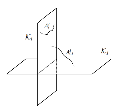
In this case, the associated matrix algebra decomposes as
| (5.13) |
As a result, the potentials between different pair of branes can be computed by considering the appropriate Hilbert spaces. The decomposition (5.13) leads to two distinct types of fluctuations. On the one hand, when the fluctuations taking values in , they can be interpreted as open strings starting and ending on the same brane . On the other hand, taking values in can be interpreted as open strings stretching between two different branes and . In that case, the fluctuation takes values in the bi-fundamental representation of .
Using the decomposition (5.13), the
inner product acquires various contributions from diagonal and off-diagonal blocks.
This can be evaluated quite concretely for taking values in the unbroken gauge sector
, i.e. the commutant of , with generators .
Scenario A: Point branes. Consider the case where consists of coinciding point branes. Then the unbroken gauge sector gets enhanced to
| (5.14) |
leading to an unbroken Yang-Mills gauge sector, which may be interpreted as color.
Furthermore, and , so that . Therefore,
| (5.15) |
This is to be expected, since there is no one-loop renormalization of the Yang-Mills coupling in the ordinary SYM, i.e. when is trivial.
Thus, the associated coupling of -YM is given by the bare coupling (3.14).
Scenario B: A stack of point branes and a bulk brane. Now consider a stack of (coinciding) point branes denoted as and a large brane . Generalizing the previous case, the unbroken gauge algebra is now . We can then evaluate as
| (5.16) |
which is proportional to the Killing form on up to some constant
| (5.17) |
We will use the normalization and choose an adapted Gell-Mann basis which include the generators in . Then,
| (5.18) |
Due to string modes linking point branes with , there is a non-trivial contribution to . To compute this, we take some as above, and evaluate the contribution from string modes connecting the point with through a coherent state on . Since act only on , we have
| (5.19) |
The integral over the string modes in the geometric trace formula (2.36) amounts to an integral over points and a sum over discrete points . The latter can be evaluated as
| (5.20) |
Now the trace over the large brane can be evaluated using (2.36) if the geometry of is known explicitly, which gives
| (5.21) |
Note that we integrate over dimensionless variables, and all scales are exhibited explicitly. It is also useful recalling that and is the curvature radius of the branes, and from the Bohr-Sommerfeld quantization condition (2.27).
Putting this together, the unbroken -sector contributes an amount
| (5.22) |
to the total one-loop effective action of the -YM theory. We can compute quite explicitly using (5.21) and assuming of order . In particular,
| (5.23a) | ||||||
| (5.23b) | ||||||
| (5.23c) | ||||||
for large .
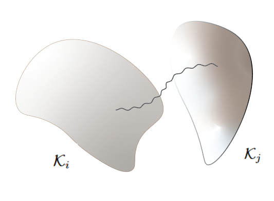
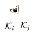
Scenario C: Large (extended) branes. Now consider the case where consists of a number of large branes . For simplicity, we restrict ourselves to the case of two large branes with associated Hilbert spaces cf. (5.12). This sector receives significant contributions due to the long/heavy open string modes linking with for being coherent states on each brane.
The unbroken gauge group in this case is generated by , where the subscripts indicate the associated branes. Note that the inner product cf. (5.11) for can be evaluated as
| (5.24) |
Furthermore, unlike scenario B), the normalization for the generators in this case is given by
| (5.25) |
Analogously to (5.17), we write
| (5.26) |
Then the geometric trace formula yields
| (5.27) |
Since will be large as and are large, the effective couplings (5.30) associated with this sector will typically be suppressed in the low-energy regime.
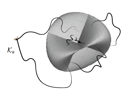
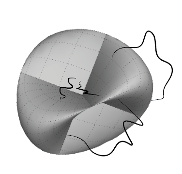
Scenario D: Self-intersecting branes. The formula (5.27) can essentially be used also for self-intersecting branes such as squashed cf. [53], where the intersecting sheets of these type of branes play (approximately) the role of different . There are also contributions from (almost-) zero modes arising as string modes . Here, are the associated coherent states located at the intersection of the different sheets of the brane. They may be significant because does not necessarily vanish at the intersection locus. Such considerations may be relevant to construct analogs of or bosons, since chiral fermions taking values in the bi-fundamental representations of arise naturally at the intersections.
Effective coupling.
Combining the one-loop contribution (for various cases above) with the classical action, we obtain the effective181818Recall that since the underlying theory is UV finite, no renormalization procedure is required. action of the quantum -Yang-Mills theory as
| (5.28) |
where
Then the effective coupling constant for the quantum Yang-Mills theory induced by the IKKT matrix model reads
| (5.29) |
or equivalently
| (5.30) |
Discussion.
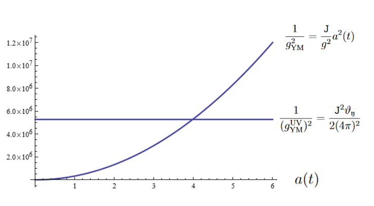
To understand the significance of (5.30), we recall that cf. (2.22) increases with the cosmic expansion. Therefore, for sufficiently early times, the renormalized coupling is dominated by the 1-loop contribution and is approximately constant. More specifically, it is much smaller than the bare coupling . At some characteristic time in the cosmic evolution, both the bare and 1-loop contributions become equal. Afterward, the bare action starts to dominate, so that the effective coupling decreases in time.191919Analogous effects can be expected for the gravitational sector of the matrix model, cf. [6].
6 Massive (higher-spin) YM gauge fields at one loop
Recall that, on a background, all fluctuations in the IKKT model are part of some (truncated) tower of higher-spin modes, which arise from a “hidden” factor of . However, massless higher-spin YM gauge fields would be phenomenologically unacceptable, since they would interact significantly and be generated in all sorts of scattering processes. Therefore, there should be some mechanism for the fields in the unbroken gauge sector to acquire mass, so that we are not in conflict with no-go theorems [50, 51]. We shall exhibit such a mechanism in this section, via quantum effects.
As a first hint towards such a mechanism, we observe that the higher-spin fields in -YM theory typically carry all dof. of massive fields [17, 16]. Hence, it is natural to expect them to acquire mass in some way. We will show that all (higher-spin) Yang-Mills gauge fields indeed acquire mass at one loop in the presence of . These quantum effects should not be confused with the standard Higgs mechanism, since it arises only at quantum level. Note that these “quantum” mass arises even for the unbroken sector of the gauge group, and comprises a priori contributions with both signs.
While the present mechanism allows us to avoid no-go theorems, we observe that the mass of the lowest-spin YM gauge bosons is larger than their siblings. This is somewhat disappointing, since we can then no longer use the present setting to reproduce the standard massless Yang-Mills gauge theory. It remains to be seen whether this issue can be circumvented by other mechanisms202020One possibility is to consider the minimal quantum space with , which will be elaborated elsewhere..
To obtain the induced mass term, consider a -valued field with internal spin- represented as
| (6.1) |
where the index in is dropped for better readability. We observe that there are two contributions to the mass term:
-
•
The first contribution arises from the kinetic term in the one-loop effective action cf. (4.13) expanded to second order in fluctuations. This contribution leads to almost the same mass for the lowest-spin and higher-spin fields. Since the mass induced by this contribution is typically very large, certain type of brane configurations are more favorable than the others.
-
•
The second arises from the contribution for pure -valued flux. This contribution sets the -valued fields apart from their lowest-spin counterparts, but in the ”wrong“ direction. In particular, the mass induced by -valued flux is negative, which can only be stabilized by the contributions coming from the kinetic term.
6.1 Kinetic contribution
We start with the first contribution to the mass term, obtained from the quadratic term in from an expansion of around . In this background, the space-time matrix d’Alembertian operator gets shifted to
| (6.2) |
where is the bare (3+1)-dimensional d’Alembert operator. Note that acts non-trivially on both and sectors. Furthermore, the can be considered as commutative functions at late times (cf. Appendix A). Then,
| (6.3) |
The trace in (4.13) including can be evaluated by noting that
| (6.4) |
where the are normalized as in (3.9). Here, is some operator assumed to act trivially on the -modes to a good approximation. This amounts to the replacement
| (6.5) |
Combining the above results, we obtain from (4.13)
| (6.6) |
using (A.3). To cast the mass terms in more standard form, we rewrite using the frame in terms of a one-form valued field as in (3.2). This gives
| (6.7) |
recalling (2.21). Assuming that takes values in some unbroken gauge algebra cf. Section 5, then
| (6.8) |
using - invariance, where
| (6.9) |
is the Casimir of acting in the adjoint on . Then (6.1) leads to the following contribution to the effective action
| (6.10) |
with the induced mass for the -valued gauge fields is given by
| (6.11) |
assuming as usual. Note that is real since the integral over produces another factor of , and it has the correct dimension since has dimension . Here,
| (6.12) |
which will also govern the scalar potential. Integrating over and keeping only the term, we obtain212121Note that this would vanish for trivial , i.e. without fuzzy extra dimensions .
| (6.13) |
where . The trace over can now be evaluated using the geometric trace formula. To be specific, we will consider the following two scenarios:
- A)
-
B)
a stack of coincident large bulk branes.
Both cases lead to an unbroken gauge algebra identified as the conventional “color”,222222At the classical level, this gauge theory would comprise a tower of -valued massless higher-spin color gauge fields, which is phenomenologically unacceptable. but the generators are small as functions in A), but large as functions in B). This leads to some qualitatively different behavior.
Scenario A. In this case, the off-diagonal string modes linking the point branes and will lead to
| (6.14) |
recalling that where is the scale of non-commutativity on .
The explicit value for this induced mass depends significantly on the structure of . We can estimate its value depending on the dimension of as follows
| (6.15a) | ||||||
| (6.15b) | ||||||
| (6.15c) | ||||||
assuming large , and recalling . Here is a characteristic KK scale on (2.29), and therefore assumed to be in the UV regime from the space-time point of view. We observe that for , the integral in (6.13) is dominated by local contributions, and therefore almost vanishes for (anti-) self-dual , since the contribution to the mass from very long strings on is small. This scenario is realized for self-intersecting 4-dimensional branes such as [53]. Then the 1-loop contributions to the -valued gauge bosons is small, both for conventional and -valued gauge fields.
Scenario B. Consider coincident large branes . The unbroken algebra is generated by where is the projector on brane . We observe that all strings starting and ending on the same brane commute with and therefore drop out. Hence, the non-trivial modes contributing to consist of string modes linking different branes th with th, which satisfy etc. Then provides a on such string modes. As such, we obtain
| (6.16) |
where the integral is over a pair of the branes under consideration. The scale of this mass can be estimated as in (6.15), but there will be an extra overall factor due to the double integral.
We recall that the above calculations apply to all modes, since the can be considered as classical functions. There is no significant distinction between the -sector and the -sector from the kinetic contribution.
6.2 Flux contribution
Now consider the contribution of the flux term to the mass. We can assume that where is constant, and are polynomials of order in . For , it follows immediately that drops out from , so that the induced mass vanishes. This means the flux contribution distinguishes the sector from the conventional sector. However, this contribution is shown to go in the wrong direction as alluded to in the above. For simplicity, consider case where . Then,
| (6.17) |
where for convenience, we recall that232323For further information, see Appendix A.2.
| (6.18) |
Here, the middle terms in (6.2) lead to the desired mass term in , while the last term will drop out. Therefore, if we are interested in estimating the magnitude of the mass term, then effectively
| (6.19) |
As a result,
| (6.20) |
where contributions are subleading. Note that the above two terms have opposite signs. In particular,
| (6.21) |
where contains the Casimir of with standard normalization. Using various relations in Appendix A, we can simplify the above to
| (6.22) |
where we have restricted ourselves to the reference point where . Note that
| (6.23) |
Then, from (5.8), we obtain the following contribution to the effective action
| (6.24) |
As always, the trace can be evaluated using (4.11). If are generators in the unbroken gauge group with low rank, then both and will give contributions with comparable strength. Then, clearly the second term dominates at late times. Its contribution is found to be
| (6.25) |
which is significant and negative. A similar formula will also apply to . Of course, the background is consistent iff the overall mass for all modes is positive or zero. This can be achieved by adding the positive mass contribution induced by the operator cf. (6.11), which applies to all spins .
6.3 Effective mass
It is important to note that the above and are not yet the physical mass, since the kinetic term is not yet appropriately normalized. With this in mind, the effective mass of the lowest-spin fields is therefore
| (6.26) |
while the effective mass of their siblings read
| (6.27) |
which we assume to be small. Assuming that the (positive) 1-loop contribution (6.14) dominates, the physical mass of ordinary YM gauge field is given by
| (6.28) |
Let us consider a similar scenario as in Fig. 6. Then, the behavior of in the early and late-time period of can be summarized as
| early period of | late-time period of |
We conclude that all color gauge bosons of -IKKT acquire masses in the presence of a large brane , with the mass scale set by the KK scales of .
Discussion.
In contrary to what one might hope, the -valued gauge fields do not seem to decouple at low energy. Furthermore, the conventional lowest-spin gauge fields turn out to acquire a mass which is larger than the -valued siblings, which is certainly not desirable from a physics point of view.242424There is another contribution from terms , which comes from the non-commutative -sector of the model that leads to the induced Einstein-Hilbert term [5]. However, we do not expect that this contribution will change the conclusion of our analysis, given that gravitational interaction is much weaker at low-energy regime. This result suggests that the lowest-spin gauge fields are indeed massive, with 3 physical degrees of freedom252525this is not in conflict with the result in [17] where massless fields were assumed for the physical Hilbert space, without quantum corrections. The no-ghost statement in [17] is expected to apply also in the massive case, due to the Yang-Mills form of the action and the physical state constraint. as in Proca theory. Therefore, the low-energy limit of the -YM theory considered in this work is not ordinary Yang-Mills theory.
7 Scalar sector and stability of
In this final section, we consider the one-loop contributions to the effective potential between disconnected sectors of the extra dimensions , which are important to understand the stabilization of and possible Higgs potentials at low energy. We observe that with does not shrink to a point, thanks to an intricate interaction between and the flux bundle over .
Scalar potential at one loop.
The one-loop effective potential for the scalar sector can again be extracted from the general formula (4), where the background associated with is now unperturbed. Namely, we will turn off the Yang-Mills fields. As a result, we have
| (7.1) |
so that
| (7.2) |
thereby defining the effective potential . This was considered as a function of the KK scale in [6] truncated at , which leads to a stabilization of . We will now study this expression more generally. To proceed, we will again assume that the background is slowly varying such that . Moreover, we can also approximate since these IR masses scale as . Then,
| (7.3) |
Here the trace over the modes just gives an overall factor , and was defined in (6.1). Using the geometrical trace formula (2.36), the trace over can be evaluated as
| (7.4) |
where encodes the symplectic structure of evaluated at the two ends of the string. Note that we have rescaled so that we only need to integrate over dimensionless variables. Therefore, (7.4) becomes
| (7.5) |
Let us now consider
| (7.6) |
in more detail. This formula applies for large branes , which are well approximated by their semi-classical geometry. We can now diagonalize with a suitable rotation such that is block-diagonal:
| (7.7) |
where indicates a Pauli matrix. Choosing an appropriate basis for the -matrices as in [52], we obtain
| (7.8a) | ||||
| (7.8b) | ||||
Intriguingly, we observe the following remarkable identity
| (7.9) |
where . This starts at order in agreement with (6.1), which reflects maximal SUSY. We also notice that if the rank of is four (e.g. ), then this simplifies as
| (7.10) |
which is indeed positive (semi-)definite. We may write the leading term as
| (7.11) |
where
| (7.12) |
Carrying out the integral over , the one-loop contribution to the effective potential262626Note that this is the 1-loop effective potential in SYM for semi-classical background configurations. is obtained as
| (7.13) |
Note that the above integrals over the positions do not localize for branes with dimension larger or equal to 4, i.e. they range over the entire brane . However, they are always finite since is compact272727 We recall that has dimension while are dimensionless. The symplectic volume integrals themselves are dimensionless numbers, cf. (2.27). Therefore, the above potential has dimension , as it should be.. For smaller branes such as point branes, the above trace needs to be evaluated explicitly; this will be discussed below.
For illustrative purpose, let us consider a few cases where has a simple form.
-
•
If has rank-2, then is positive, leading to a negative potential. However, it is expected that this case is too degenerate.
-
•
In the case where or is rank-4, is again positive, leading to a negative potential and suggesting a bound state. This case will be discussed in more detail below.
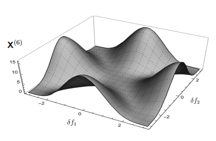
Figure 7: A generic form for if is rank-4. -
•
Finally, consider the case where is rank-6. For simplicity, suppose . Then, and has the form of Fig 8.
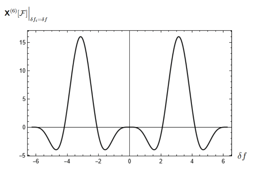
Figure 8: where In this case, some finite repulsive force between branes may arise due to .
7.1 Examples of scalar potentials
Point branes.
For point branes with , we simply have , thus . This is to be expected, because the theory locally reduces to (a extension of) SYM.
A point brane and a bulk brane.
Consider a point brane located at and a large brane centered at the origin. Then their interaction is mediated by the integral over string modes stretching between these branes. The effective potential is
| (7.14) |
This gives the effective potential for the point brane. Observe that the potential has a non-trivial extremum at . Furthermore, since , the point branes tend to glue to , which should lead to a color-like low-energy gauge sector. This means that the point branes are attracted to the (center of) , as desired. In fact, this will be the standard behavior of branes with dimensions lesser or equal to four.
Let us evaluate the above effective potential quantitatively by recalling that . Then, for
| (7.15a) | ||||||
| (7.15b) | ||||||
| (7.15c) | ||||||
for large . Note that since is rank-6 when , the last expression can have either sign. As a reminder, the curvature radius encodes the size of .
Intersecting flat branes.
Consider the case of two almost-flat large branes and , which may intersect each other. Then the interaction between the branes is obtained from (7.13) assuming that for each brane:
| (7.16) |
Note again that are assumed to be compact282828The integrals would be divergent for non-compact branes, so that the present result should only be used to gain a qualitative understanding.. The above integral is always negative or zero as long as due to (7.10), and vanishes only if vanishes or is (anti-) self-dual292929Namely, in the 4-dimensional case with being the Hodge dual operator on . Indeed, one can show that , which justifies the claim..
If one of the branes has dimension , then can have either sign. Indeed, consider first the numerator . We can use (7) to write
| (7.17) |
For the sake of argument, assume that has rank and has rank , so that we can replace . Then, clearly – and hence the overall interaction energy – can be either positive or negative. In particular, if , the potential is always positive.
Let us estimate (7.16) in various cases where . We assume for simplicity that the branes are orthogonal, so that and . Then, for
| (7.18) |
assuming of order and large . Observe that the integral over and is actually dominated by the long strings. Thus, the above result is only indicative for understanding the relevant scales303030In particular, this means that the contributions from (almost-) zero modes arising at the intersection are not significant and can be dropped here.. Nevertheless, the net result is always finite due to the compact nature of . Alternatively, the above computation can be carried out in terms of KK modes on , see e.g. [6] for more details. However, the present geometric evaluation is much more transparent.
Self-intersecting branes.
The above discussion applies, in particular, for self-intersecting branes such as squashed , cf. [53], which are interesting due to chiral fermions arising at their intersection.
For example, the self-intersecting sheets of can be approximated by a system of flat intersecting branes sharing a -plane, which may be written as . The open string modes between two sheets then lead to
| (7.19) |
which is expected to be negative since the flux difference on the intersection vanishes, so that has (essentially) rank 4. At the end of the day, the potential between different sheets will again be proportional to , since this is the unique UV scale of .
Note that the contributions from possible zero modes arising on self-intersecting branes are of order and can therefore be neglected. This contribution can be estimated quickly by integrating over the radial direction of a sphere of radius with the intersection of the self-intersecting brane as its origin.
7.2 -flux bundle contributions to the scalar potential
As pointed out in [54], there is another contribution to the vacuum energy on the background under consideration, which arises from the geometric background on coupling to at one loop. This leads to stabilization of , due to the non-commutativity scale of . Note that can be related to the scale of , cf. Subsection 2.2. This represents a crucial difference to ordinary SYM, which does not have any scale.
To compute this contribution, we need to take into account the -valued background flux on space-time in (4) where instead of dimensional character cf. (4.9), we will consider the dimensional one and expand it to order . Then the 1-loop potential (7) takes the form
| (7.20) |
where and with .
contribution.
Now consider the mixed term, where
| (7.21) |
since as assumed above313131Note that the space-like contributions to are strongly suppressed for and hence omitted. This would typically not be the case for the Moyal-Weyl quantum plane , which provides a dynamical mechanism in favor of .. The trace over can be evaluated as always using the geometric trace formula for . The trace over can also be evaluated using string modes, noting that when acting on a string mode on . Recalling that where is the intrinsic length scale of and are the normalized fiber coordinates of , cf. Appendix A. We obtain
| (7.22) |
where is the symplectic volume form of (2.34). The integral over results in
| (7.23) |
for large . Here, is the scale of non-commutativity on , which is approximately . On the other hand,
| (7.24) |
As a result,
| (7.25) |
using and , which provides the crucial negative slope required for a non-trivial vacuum, as elaborated below. Here, we have assumed that and replace with a 4-dimensional ball with radius of . This potential behaves as
| (7.26) |
near 0, while for large it has a mild behavior as shown in figure 10.
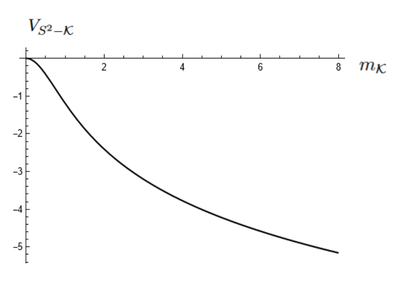
Combined with , this leads to a non-trivial minimum for as discussed in the next section, given that the downward slope of dominates at small . The crucial point we want to emphasize here is that the coupling between and the flux on space-time introduces a scale into the theory. This qualitative conclusion is unchanged by the further effects from as discussed below.
contribution.
Finally, consider the contribution from , which is given by
| (7.27) |
where . Using (7.23), we get
| (7.28) |
We can evaluate the tensorial contribution again using string modes on as
| (7.29) |
where the purely space-like contributions are subleading. Then,
| (7.30) |
for long string modes. We obtain
| (7.31) |
In terms of the magnitude, we observe that
| (7.32) |
The bottom line of this computation is that even though does contribute a binding energy323232It was assumed in [54, 9] that , which suggested a different mechanism for stabilizing . The present result using geometric trace formula seems more satisfactory., it only helps to stabilize the background, but not .
7.3 Stability of
Given the above results, we can try to address the important problem of how to stabilize . It is difficult to answer this question in full detail; thus we will merely try to understand some semi-quantitative features, and leave the complete analysis for future work.
The stability of is determined by the condition that the 1-loop effective potential
| (7.33) |
should have a non-trivial (global or local) minimum, which is negative. Here,
| (7.34) |
Note that around , . Then, to ensure global stability, we will assume that the classical potential dominates over the 1-loop potentials for large , i.e. , which is a very reasonable requirement in the weak coupling regime under consideration. The non-trivial local minimum for arises from the negative contribution in . In summary, has the following shape:
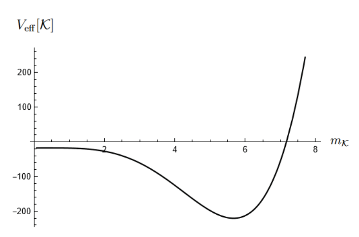
The reader may notice that the structure of is largely determined by the non-abelian sector of the theory, while the coupling to is essential for stabilizing the radial scale. Furthermore, the interaction potential between two branes is attractive, provided the “effective” embedding dimensions less than or equal to 4. This strongly suggests the existence of stable branes with non-trivial sub-structure, as considered in this paper. Determining their specific structures would require much more detailed work.
8 Discussion
This work contains several significant new results, which should provide the basis for further investigations of the physics in the matrix model framework. The first important (but rather disappointing) result is the mechanism described in Section 6, which induces mass for all (unbroken) -valued gauge fields from quantum effects in the presence of . While this mechanism allows -YM to avoid no-go theorems [50, 51], it does not lead to near-realistic physics333333One possibility to circumvent this issue is to consider the minimal quantum space with . This will be elaborated elsewhere.. Note, however, that the time-dependent effective couplings of -YM at one loop do show reasonable behavior (cf. Fig. 6).
A further important result is the scalar potential at one loop, which allows for the stabilization of . This is also essential for obtaining an induced Einstein-Hilbert term and gravity in the present framework, along the lines of [5, 6, 9]. It turns out that the scalar potential indeed acquires a non-trivial minimum for a non-vanishing radius of suitable , with scale inherited from the non-commutativity scale of the cosmological space-time . The methods developed here provide the basis to determine the dynamically preferred structure of the compact extra dimensions , which should be elaborated in future work. The crucial point we want to emphasize here is that the superconformal symmetry of the SYM sector in -YM is broken by the quantum spacetime. This provides an essential ingredient for obtaining interesting physics.
Finally, we have computed the 1-loop corrections to the Yang-Mills coupling constants. All of these calculations rely crucially on a basic trace formula based on coherent states, which provides a suitable way to perform loop computations, despite the complexity of the model under consideration. These techniques will certainly be useful also in other contexts, and provide an important step towards identifying more realistic backgrounds in the matrix model.
Some further comments are in order, to clarify the relation of the present work with other approaches. The UV finiteness of the higher-spin gauge theory induced by the IKKT matrix model on the background brane is essential for the loop computations, based on to maximally supersymmetry and the fuzzy nature of . This is quite different with standard massless higher-spin gravities, see e.g. [55, 56, 57, 58, 59, 60, 61] where one typically needs to provide some regularization scheme. The present matrix model setting also differs from the conventional approach to string theory, where target space is compactified; this is not the case here. Furthermore, the mechanism of induced masses found in this work should allow obtaining a complete effective theory for massive higher-spin fields where all vertices can be derived by averaging over . It would also be interesting to compare interacting vertices of -IKKT with recent attempts of constructing Lorentz-invariant vertices of massive fields in e.g. [62, 63, 64].
Acknowledgement
We thank Tim Adamo and Zhenya Skvortsov for enlightening discussion. TT thanks the Simons Foundation for the hospitality during the annual meeting on Celestial Holography in Newyork, where the final stage of this work was in completion. This work is supported by the Austrian Science Fund (FWF) grant P36479.
Appendix A Supplemental material
A.1 Useful relations
This appendix provides additional relations extracted from [65, 17, 16] for used in the main text. We have
| (A.1a) | ||||
| (A.1b) | ||||
| (A.1c) | ||||
| (A.1d) | ||||
| (A.1e) | ||||
| (A.1f) | ||||
which are frequently used in the main text. Here are the generators of acting on , and is an intrinsic length scale on . At late times, we have
| (A.2) |
which is dominated by the space-time components of size
| (A.3) |
It is useful to introduce normalized generators
| (A.4) |
Then
| (A.5) |
A.2 The structure of the higher-spin sphere
At some given reference point where , the generators are space-like due to (A.1a), and therefore the can be used to parametrize the internal 2-sphere . Even though that sphere has symplectic measure (2.34) with volume
| (A.6) |
reminiscent of a fuzzy sphere and thus admitting only spherical harmonics truncated343434The truncation of spin can be understood in terms of the angular momentum operators acting on the internal at the given reference point, see [65] for a detailed discussion. This cannot be separated from the underlying globally, reflecting the Poisson structure on which is dominated by . A careful computation of the symplectic form on [66] reproduces indeed (A.6), confirming the cutoff on . at spin , the are very different from standard fuzzy sphere generators. In particular,
| (A.7) |
are not the inverse of the symplectic form but are suppressed by a large factor . This implies that for late times , the are effectively commutative. For example, the Poisson brackets
| (A.8) |
coincide with those on a fuzzy sphere with radius 1, but are suppressed by a factor . Equivalently, the brackets of coincide with those of a fuzzy sphere of radius , but describe a sphere with radius (A.1b). Hence the should be thought of as (compactified) momentum generators on with a small admixture fuzzy sphere generators . This justifies the simplification in the main text.
A.3 Some loop integrals
We need the following integral arising in the 1-loop effective action
| (A.9) |
for some function on , where , and we define
| (A.10) |
by integrating first over via a contour rotation .
References
- [1] N. Ishibashi, H. Kawai, Y. Kitazawa and A. Tsuchiya, A Large N reduced model as superstring, Nucl. Phys. B 498 (1997) 467–491 [hep-th/9612115].
- [2] H. C. Steinacker, On the quantum structure of space-time, gravity, and higher spin in matrix models, Class. Quant. Grav. 37 (2020), no. 11 113001 [1911.03162].
- [3] H. C. Steinacker, Quantum Geometry, Matrix Theory, and Gravity. Cambridge University Press, 4, 2024.
- [4] T. Anous, J. L. Karczmarek, E. Mintun, M. Van Raamsdonk and B. Way, Areas and entropies in BFSS/gravity duality, SciPost Phys. 8 (2020), no. 4 057 [1911.11145].
- [5] H. C. Steinacker, Gravity as a quantum effect on quantum space-time, Phys. Lett. B 827 (2022) 136946 [2110.03936].
- [6] H. C. Steinacker, One-loop effective action and emergent gravity on quantum spaces in the IKKT matrix model, 2303.08012.
- [7] A. D. Sakharov, Vacuum quantum fluctuations in curved space and the theory of gravitation, Dokl. Akad. Nauk Ser. Fiz. 177 (1967) 70–71.
- [8] E. Battista and H. C. Steinacker, One-loop effective action of the IKKT model for cosmological backgrounds, 2310.11126.
- [9] K. Kumar and H. C. Steinacker, Modified Einstein equations from the 1-loop effective action of the IKKT model, 2312.01317.
- [10] S.-W. Kim, J. Nishimura and A. Tsuchiya, Expanding (3+1)-dimensional universe from a Lorentzian matrix model for superstring theory in (9+1)-dimensions, Phys. Rev. Lett. 108 (2012) 011601 [1108.1540].
- [11] K. N. Anagnostopoulos, T. Azuma, K. Hatakeyama, M. Hirasawa, Y. Ito, J. Nishimura, S. K. Papadoudis and A. Tsuchiya, Progress in the numerical studies of the type IIB matrix model, 10, 2022. 2210.17537.
- [12] J. Nishimura and A. Tsuchiya, Complex Langevin analysis of the space-time structure in the Lorentzian type IIB matrix model, JHEP 06 (2019) 077 [1904.05919].
- [13] H. C. Steinacker, Cosmological space-times with resolved Big Bang in Yang-Mills matrix models, JHEP 02 (2018) 033 [1709.10480].
- [14] H. Aoki, N. Ishibashi, S. Iso, H. Kawai, Y. Kitazawa and T. Tada, Noncommutative Yang-Mills in IIB matrix model, Nucl. Phys. B 565 (2000) 176–192 [hep-th/9908141].
- [15] J. Madore, S. Schraml, P. Schupp and J. Wess, Gauge theory on noncommutative spaces, Eur. Phys. J. C 16 (2000) 161–167 [hep-th/0001203].
- [16] M. Sperling and H. C. Steinacker, Covariant cosmological quantum space-time, higher-spin and gravity in the IKKT matrix model, JHEP 07 (2019) 010 [1901.03522].
- [17] H. C. Steinacker, Higher-spin kinematics & no ghosts on quantum space-time in Yang-Mills matrix models, 1910.00839.
- [18] H. C. Steinacker and T. Tran, Soft limit of higher-spin interactions in the IKKT model, 2311.14163.
- [19] H. C. Steinacker and T. Tran, Spinorial description for Lorentzian -IKKT, 2312.16110.
- [20] R. R. Metsaev, Poincare invariant dynamics of massless higher spins: Fourth order analysis on mass shell, Mod. Phys. Lett. A 6 (1991) 359–367.
- [21] R. R. Metsaev, S matrix approach to massless higher spins theory. 2: The Case of internal symmetry, Mod. Phys. Lett. A 6 (1991) 2411–2421.
- [22] D. Ponomarev and E. D. Skvortsov, Light-Front Higher-Spin Theories in Flat Space, J. Phys. A 50 (2017), no. 9 095401 [1609.04655].
- [23] D. Ponomarev, Chiral Higher Spin Theories and Self-Duality, JHEP 12 (2017) 141 [1710.00270].
- [24] E. D. Skvortsov, T. Tran and M. Tsulaia, Quantum Chiral Higher Spin Gravity, Phys. Rev. Lett. 121 (2018), no. 3 031601 [1805.00048].
- [25] R. R. Metsaev, Light-cone gauge cubic interaction vertices for massless fields in AdS(4), Nucl. Phys. B 936 (2018) 320–351 [1807.07542].
- [26] R. R. Metsaev, Cubic interactions for arbitrary spin -extended massless supermultiplets in 4d flat space, JHEP 11 (2019) 084 [1909.05241].
- [27] M. Tsulaia and D. Weissman, Supersymmetric Quantum Chiral Higher Spin Gravity, 2209.13907.
- [28] A. Sharapov, E. Skvortsov, A. Sukhanov and R. Van Dongen, Minimal model of Chiral Higher Spin Gravity, 2205.07794.
- [29] A. Sharapov and E. Skvortsov, Chiral Higher Spin Gravity in (A)dS4 and secrets of Chern-Simons Matter Theories, 2205.15293.
- [30] A. A. Tseytlin, On limits of superstring in AdS(5) x S**5, Theor. Math. Phys. 133 (2002) 1376–1389 [hep-th/0201112].
- [31] A. Y. Segal, Conformal higher spin theory, Nucl. Phys. B 664 (2003) 59–130 [hep-th/0207212].
- [32] X. Bekaert, E. Joung and J. Mourad, Effective action in a higher-spin background, JHEP 02 (2011) 048 [1012.2103].
- [33] H. C. Steinacker, Quantized open FRW cosmology from Yang–Mills matrix models, Phys. Lett. B 782 (2018) 176–180 [1710.11495].
- [34] M. P. Blencowe, A Consistent Interacting Massless Higher Spin Field Theory in = (2+1), Class. Quant. Grav. 6 (1989) 443.
- [35] E. Bergshoeff, M. P. Blencowe and K. S. Stelle, Area Preserving Diffeomorphisms and Higher Spin Algebra, Commun. Math. Phys. 128 (1990) 213.
- [36] C. N. Pope and P. K. Townsend, Conformal Higher Spin in (2+1)-dimensions, Phys. Lett. B 225 (1989) 245–250.
- [37] E. S. Fradkin and V. Y. Linetsky, A Superconformal Theory of Massless Higher Spin Fields in = (2+1), Mod. Phys. Lett. A 4 (1989) 731.
- [38] A. Campoleoni, S. Fredenhagen, S. Pfenninger and S. Theisen, Asymptotic symmetries of three-dimensional gravity coupled to higher-spin fields, JHEP 11 (2010) 007 [1008.4744].
- [39] M. Henneaux and S.-J. Rey, Nonlinear as Asymptotic Symmetry of Three-Dimensional Higher Spin Anti-de Sitter Gravity, JHEP 12 (2010) 007 [1008.4579].
- [40] M. R. Gaberdiel and R. Gopakumar, An AdS3 Dual for Minimal Model CFTs, Phys. Rev. D 83 (2011) 066007 [1011.2986].
- [41] M. R. Gaberdiel and R. Gopakumar, Minimal Model Holography, J. Phys. A 46 (2013) 214002 [1207.6697].
- [42] M. R. Gaberdiel and R. Gopakumar, Higher Spins & Strings, JHEP 11 (2014) 044 [1406.6103].
- [43] M. Grigoriev, I. Lovrekovic and E. Skvortsov, New Conformal Higher Spin Gravities in , JHEP 01 (2020) 059 [1909.13305].
- [44] M. Grigoriev, K. Mkrtchyan and E. Skvortsov, Matter-free higher spin gravities in 3D: Partially-massless fields and general structure, Phys. Rev. D 102 (2020), no. 6 066003 [2005.05931].
- [45] M. Sperling and H. C. Steinacker, Intersecting branes, Higgs sector, and chirality from = 4 SYM with soft SUSY breaking, JHEP 04 (2018) 116 [1803.07323].
- [46] H. C. Steinacker and J. Tekel, String modes, propagators and loops on fuzzy spaces, JHEP 06 (2022) 136 [2203.02376].
- [47] T. Adamo and T. Tran, Higher-spin Yang-Mills, amplitudes and self-duality, 2210.07130.
- [48] T. Tran, Toward a twistor action for chiral higher-spin gravity, 2209.00925.
- [49] Y. Herfray, K. Krasnov and E. Skvortsov, Higher-Spin Self-Dual Yang-Mills and Gravity from the twistor space, 2210.06209.
- [50] S. Weinberg, Photons and Gravitons in -Matrix Theory: Derivation of Charge Conservation and Equality of Gravitational and Inertial Mass, Phys. Rev. 135 (1964) B1049–B1056.
- [51] S. R. Coleman and J. Mandula, All Possible Symmetries of the S Matrix, Phys. Rev. 159 (1967) 1251–1256.
- [52] D. N. Blaschke and H. Steinacker, On the 1-loop effective action for the IKKT model and non-commutative branes, JHEP 10 (2011) 120 [1109.3097].
- [53] H. C. Steinacker, One-loop stabilization of the fuzzy four-sphere via softly broken SUSY, JHEP 12 (2015) 115 [1510.05779].
- [54] H. C. Steinacker, Quantum Geometry, Matrix Theory, and Gravity. Cambridge University Press, 4, 2024.
- [55] S. Giombi and I. R. Klebanov, One Loop Tests of Higher Spin AdS/CFT, JHEP 12 (2013) 068 [1308.2337].
- [56] S. Giombi, I. R. Klebanov and B. R. Safdi, Higher Spin AdSd+1/CFTd at One Loop, Phys. Rev. D 89 (2014), no. 8 084004 [1401.0825].
- [57] S. Giombi, I. R. Klebanov and A. A. Tseytlin, Partition Functions and Casimir Energies in Higher Spin AdSd+1/CFTd, Phys. Rev. D 90 (2014), no. 2 024048 [1402.5396].
- [58] M. Beccaria and A. A. Tseytlin, On higher spin partition functions, J. Phys. A 48 (2015), no. 27 275401 [1503.08143].
- [59] M. Beccaria, X. Bekaert and A. A. Tseytlin, Partition function of free conformal higher spin theory, JHEP 08 (2014) 113 [1406.3542].
- [60] J.-B. Bae, E. Joung and S. Lal, One-loop test of free SU(N ) adjoint model holography, JHEP 04 (2016) 061 [1603.05387].
- [61] M. Günaydin, E. D. Skvortsov and T. Tran, Exceptional higher-spin theory in AdS6 at one-loop and other tests of duality, JHEP 11 (2016) 168 [1608.07582].
- [62] N. Arkani-Hamed, T.-C. Huang and Y.-t. Huang, Scattering amplitudes for all masses and spins, JHEP 11 (2021) 070 [1709.04891].
- [63] R. R. Metsaev, Interacting massive and massless arbitrary spin fields in 4d flat space, Nucl. Phys. B 984 (2022) 115978 [2206.13268].
- [64] L. Cangemi, M. Chiodaroli, H. Johansson, A. Ochirov, P. Pichini and E. Skvortsov, From higher-spin gauge interactions to Compton amplitudes for root-Kerr, 2311.14668.
- [65] M. Sperling and H. C. Steinacker, The fuzzy 4-hyperboloid and higher-spin in Yang–Mills matrix models, Nucl. Phys. B 941 (2019) 680–743 [1806.05907].
- [66] E. Broukal, Spherically symmetric geometries in the framework of matrix models, .