Quantum annealing for finding maximum-weight independent set of unit-disk graphs

Abstract

Recent progress in quantum computing and quantum simulation of many-body systems with arrays of neutral atoms using Rydberg excitation brought unforeseen opportunities towards computational advantage in solving various optimization problems. The problem of maximum-weight independent set (MWIS) of unit-disk graphs is an example of NP-hard optimization problems. It involves finding the largest set of vertices with the maximum sum of their weights for a graph which has edges connecting all pairs of vertices within a unit distance. This problem can be solved using quantum annealing with an array of interacting Rydberg atoms. For a particular graph, a spatial arrangement of atoms represents vertices of the graph, while the detuning from the resonance at Rydberg excitation defines weights of these vertices. The edges of the graph can be drawn according to the unit disk criterion. MWIS can be obtained by applying a variational quantum adiabatic algorithm (VQAA). We consider driving the quantum system of interacting atoms to the many-body ground state using a non-linear quasi-adiabatic profile for sweeping the Rydberg detuning. We also propose using a quantum wire which is a set of auxiliary atoms of a different chemical element to mediate strong coupling between the remote vertices of the graph. We investigate this effect for different lengths of the quantum wire. We also investigate the quantum phases of matter realizing commensurate and incommensurate phases in 1D and 2D spatial arrangement of the atomic array.

I Introduction

In the realm of computer science [1] there is a class of non-deterministic polynomial-time (NP)-hard problems that are notoriously challenging to solve efficiently. The algorithms designed for classical computers struggle to find solutions of such problems within a reasonable time frame/cost. With development of the capabilities of quantum computing technologies there is a growing interest in finding useful applications of near-term quantum machines [2]. Recent achievements in this field allowed further exploration of the possibility of finding solutions of a number of NP-hard problems [3, 4, 5]. In particular, recently it has been proposed to implement a quantum annealer with heteronuclear ultracold Rydberg atoms in optical lattices, featuring a highly controllable environment to explore the many-body adiabatic passage [6].

In graph theory [7] we define a graph $G(V,E)$ with $V$ set and $E$ edges. A graph is called planar, if its vertices are embedded in the plane and its edges are not intersecting. Non-planar graphs represent a class of graphs where the edges between some of the vertices are intersecting and the vertices can be represented in three-dimensional space. A subset $S$ of a set $V$ is called an independent set if there are no couples of vertices of $S$ which are connected by edge $E$. If there is no larger independent set $S^{\prime}$ with $|S^{\prime}|>|S|$, then $S$ is a maximum independent set (MIS). In other words, the size of the maximum independent set is the cardinality (number of vertices) of the largest independent set of the graph. Assigning a weight $w_{v}>0$ to each vertex $v\in V$ generalizes the MIS problem to a maximum-weight independent set (MWIS) problem, which can be solved by finding the independent set with the total weight $W=\sum_{v\in V}w_{v}$. Finding the solution for MIS or MWIS is an NP-hard problem [1], meaning there is no known efficient algorithm to solve it for all possible graphs. However, there are approximate classical algorithms and heuristics that can provide good solutions in practice. Examples of weighted graphs considered in our work are presented in Fig. 1(a).

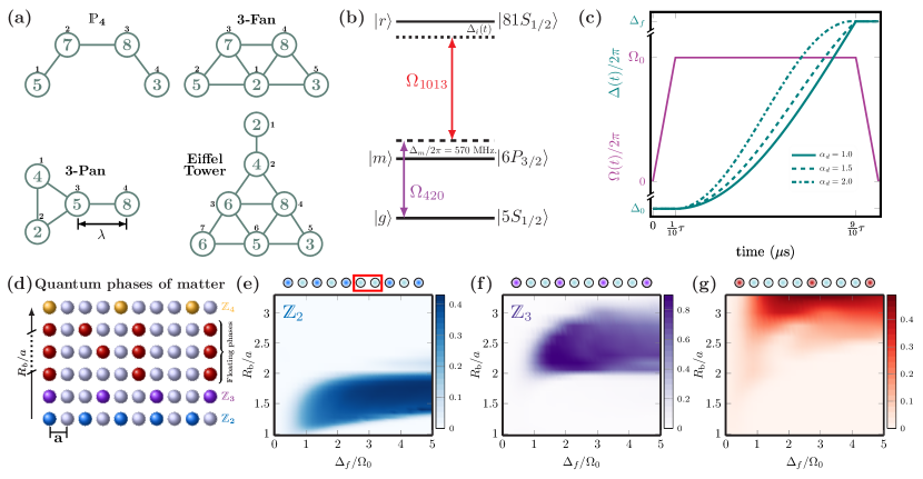
Figure 1: (a) Arbitrary undirected planar graphs being represented by Rydberg atoms. The positions of the vertices are defined as function of graph spacing constant $\lambda$ in Table 1. The labels inside the circles represent weights of the corresponding vertices. The numbers outside the circles mark the position of each vertice; (b) Scheme of the atomic energy levels and laser excitation scheme for ⁸⁷Rb atoms; (c) Time profiles of two-photon Rabi frequency $\Omega(t)$, and detuning from the Rydberg state $\Delta(t)$ for three different laser excitation courses with parameters $\alpha$ in Eq. (5) $\alpha_{d}=1.0$ (solid), $\alpha_{d}=1.7$ (dashed), and $\alpha_{d}=2.0$ (dashed-dotted). Here $\Omega_{0}/2\pi=1.75$ $\mathrm{M}\mathrm{H}\mathrm{z}$, $\Delta_{0}/2\pi=-6.0$ $\mathrm{M}\mathrm{H}\mathrm{z}$, $\Delta_{f}/2\pi=+6.0$ $\mathrm{M}\mathrm{H}\mathrm{z}$, and $\tau=5.0$ $\mu\mathrm{s}$; (d) Scheme of quantum phases of matter represented by Rydberg excitations in the atomic array (shown as colored circles) with commensurate order $\mathds{Z}_{2}$, $\mathds{Z}_{3}$, and $\mathds{Z}_{4}$ and possible incommensurate floating phases between $\mathds{Z}_{3}$ and $\mathds{Z}_{4}$; (e-g) The numerically calculated probability distributions for ordered-states $\mathds{Z}_{2}$, $\mathds{Z}_{3}$, and an incommensurate floating phase, respectively, for an array of 10 atoms arranged in 1D with lattice spacing constant $a$ ($\mu\mathrm{m}$). The red rectangle on top of graph (e) marks position of a domain wall.

Quantum computer can be used for solving both MIS and MWIS problems. Basically, there are two main approaches to drive the quantum system to the many-body ground state which reveals solution of MIS, MWIS, or other optimization problems. The first one is a quantum approximate optimization algorithm (QAOA) [8] and its hybrid quantum iterative version [9]. These algorithms can be implemented using specific properties of laser-driven atomic systems with Rydberg interactions. In this scheme laser pulses are resonant to the atomic transition, and the pulse phases and durations are varied. These variational parameters are used to generate the desired many-body evolution. The other approach is a variational quantum adiabatic algorithm (VQAA) [10, 11, 12] in which the detuning of the laser pulse exciting a Rydberg state is swept from the initial negative value to a large final positive value, while the Rabi frequency is kept constant. VQAA has shown better performance compared with QAOA [3]. A protocol for solving hard combinatorial graph problems by combining variational analog quantum computing and machine learning is assessed by quality score in Ref. [13]. A comparison of the performance of the state-of-the-art classical solvers with QAOA and VQAA for different optimization problems was reported in Ref. [14, 15]. In Ref. [16] a comprehensive study of hybrid digital-analog algorithms on Rydberg atoms is performed showing the feasibility of VQAA to the near-term realizability of quantum learning with the scalable architecture of arrays of neutral atoms.

Finding the solutions of MIS has been experimentally achieved using a homonuclear atomic architecture with quantum wires for planar graphs [4] and for non-planar graphs [17, 18], and also for a large-size graph on the King’s lattice [19]. Construction of rigorous and challenging solving instances for the MIS problem via adiabatic approach was presented in Ref. [20], and quantum optimization algorithms for finding the solutions of the MIS problem have been explored in Ref. [3]. The concept of vertex support to adjust local detunings on atoms was proposed in Ref. [21]. The framework for solving combinatorial optimization problems for non-unit disk graphs was provided for MIS and max-cut problems in Refs. [22]. The quantum devices based on programmable arrays of neutral atoms have been extensively studied to find solutions of other NP-hard problems including max-cut [5, 2, 23] and max-$k$-cut problems [24]. The performance of two algorithms on solving max-cut problem was studied and tested on IEEE 9-bus power grid graph state on Aquila quantum processor [25]. The concept of quantum wire is essential for finding solutions of other optimization problems, such as quadratic unconstrained binary optimization problem (QUBO) [26]. A generalized framework for solving MWIS, QUBO, and for integer factorization problem was discussed in Ref. [27]. A scalable architecture for solving higher-order constrained binary optimization problems was presented in Ref. [28].

Finding solutions for optimization problems as MIS/MWIS of unit disk graphs is beneficial for practical applications such as network design, scheduling tasks [29, 30], gene selection, and prediction of protein-protein interaction in bioinformatics [31].

In this paper we theoretically study the problem of finding MIS/MWIS on unit disk graphs using an array of ultracold neutral atoms and VQAA. We use a non-linear quasi-adiabatic profile of detuning from the resonance when exciting atoms into Rydberg states. We investigate commensurate $\mathds{Z}_{n}$-ordered states and incommensurate phases of matter in 1D and 2D spatial arrangement of atoms and the ability to construct a desired phase by controlling the system parameters. Next, we consider mediating interaction between far distant atoms by a quantum wire of atoms of a different chemical element. We investigated the cost of different lengths of the quantum wire.

Here we report the calculated probability distributions of many-body quantum states which reveal commensurate ordered states $\mathds{Z}_{2}$ and $\mathds{Z}_{3}$, and incommensurate phase of 1D array of atoms. We have shown that using quasi-adiabatic driving it is possible to find the solutions of MWIS of planar and non-planar unit-disk graphs. We investigated the role of the length of a quantum wire to mediate interaction between far-distant atoms, and studied the quantum phases of a graph-wire system to find solutions of MWIS.

The paper is organized as follows: in section II we discuss the Hamiltonian of the atomic system and the procedure used for annealing the system to the desired many-body ground state. We show the dynamics of the states of a laser-driven single atom and of a spatially arranged ensemble of atoms representing a graph. In section III, we study the quantum phase transition of commensurate and incommensurate phases, and discuss the ability of realizing a floating incommensurate phase. In section IV, we discuss results of MISs and MWIS for our simulation for planar graphs. In section V, we find the MISs and MWIS of a non-planar graph representing a Johnson solid $J_{14}$, which facets are different regular polygons in a three-dimensional array. The use of a heteronuclear quantum wire for mediating interaction between far distant atoms is discussed in section VI.

II Quantum system

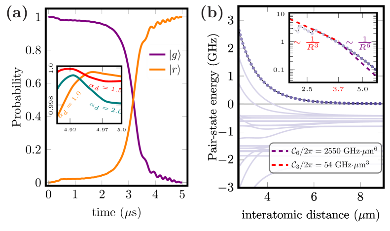
Figure 2: (a) The time dynamics of the probabilities of ground and Rydberg states during Rydberg excitation of a single atom for different values of $\alpha_{d}$; (b) The pair-state interaction energy for two ⁸⁷Rb $|81S_{1/2},m_{j}=1/2\rangle$ Rydberg atoms. Solid-teal curves are the eigenenergies of the interaction matrix after diagonalisation, calculated using Alklai Rydberg calculator (ARC) [32], with $\theta=0$, $\phi=0$, $\delta n=2$, $\delta l=1$. Dashed curves are the fitting approximation for short-range dipole-dipole (red) and long-range van der Waals (violet) regimes, showing that $\mathcal{C}_{3}/2\pi=54$ $\mathrm{G}\mathrm{H}\mathrm{z}$$\cdot$$\mu\mathrm{m}^{3}$, $\mathcal{C}_{6}/2\pi=2550$ $\mathrm{G}\mathrm{H}\mathrm{z}$$\cdot$$\mu\mathrm{m}^{6}$, $R_{\text{\tiny LR}}=2.0$ $\mu\mathrm{m}$ and $R_{\text{\tiny vdW}}=3.7$ $\mu\mathrm{m}$. The inset shows the log-log plot of the fitting values and the corresponding eigenenergy.

The spatially arranged array of atoms excited into the Rydberg states can be represented by a mathematical graph $G(V,E)$ in which the vertices $V$ represent the atoms, and the edges $E$ represent pairwise interaction between atoms. The governing Hamiltonian of this system can be written as

$$\mathcal{\hat{H}}=\mathcal{\hat{H}}_{q}+\mathcal{\hat{H}}_{c},$$ (1)

where $\mathcal{\hat{H}}_{q}$ is the quantum driver Hamiltonian which is composed of off-diagonal operators, and $\mathcal{\hat{H}}_{c}$ is the cost Hamiltonian [33, 34]. Minimizing the cost parameters is an ultimate goal. The scheme of atomic energy levels is shown in Fig. 1(b). These two basic ingredients of the system Hamiltonian are given by

$$\mathcal{\hat{H}}_{q}=\frac{1}{2}\sum_{i}^{V}\bigr{[}\Omega(t)|g\rangle_{i}\langle r|+h.c.\bigr{]},$$ (2)

$$\mathcal{\hat{H}}_{c}=-\sum_{i}^{V}\Delta_{i}(t)~{}\hat{n}_{i}+\sum_{i<j}^{E}\frac{\mathcal{C}_{6}}{|R_{i}-R_{j}|^{6}}\hat{n}_{i}\hat{n}_{j}.$$ (3)

where $|g\rangle=|5S_{1/2},F=2\rangle$ is the ground state of the trapped ⁸⁷Rb atom, $|r\rangle=|81S_{1/2},m_{j}=1/2\rangle$ is the Rydberg state, and the operator $\hat{n}_{i}=|r\rangle_{i}\langle r|$ is the projector to the Rydberg state of $i^{th}$ atom. $\Omega(t)$ is a time-dependent effective two-photon Rabi frequency for $|g\rangle\to|r\rangle$ transition with the maximum value $\Omega_{0}=\dfrac{\Omega_{420}~{}\Omega_{1013}}{2\Delta_{m}}$, where $\Omega_{420}/2\pi=40$ $\mathrm{M}\mathrm{H}\mathrm{z}$, and $\Omega_{1013}/2\pi=50$ $\mathrm{M}\mathrm{H}\mathrm{z}$ are the one-photon Rabi frequencies of laser radiation which couples $|g\rangle$ to $|r\rangle$ through the intermediate state $|m\rangle=|6P_{3/2},F=2,m_{F}=2\rangle$, and $\Delta_{m}/2\pi=570$ $\mathrm{M}\mathrm{H}\mathrm{z}$ is the detuning from the intermediate state. The values of Rabi frequencies are chosen to excite single atom to Rydberg state according to the considered time scale with high fidelity. $\Delta_{i}(t)$ is the detuning from the two-photon resonance with the Rydberg state $|r\rangle$ of the atom/vertex $i$. For the MIS problem we set identical detunings for all atoms $\Delta_{i}(t)\equiv\Delta(t)$. Later, for the MWIS problem we will select detuning for each atom individually. We used the following shapes of time profiles $\Omega(t)$ and $\Delta(t)$ [see Fig. 1(c)]:

$$\Omega(t)=\left\{\begin{array}[]{ll}\Omega_{0}(\frac{t}{t_{f_{1}}}),&0\leq t\leq t_{f_{1}},\\ \Omega_{0},&t_{f_{1}}<t\leq t_{f_{2}},\\ \Omega_{0}\frac{(t-\tau)}{(t_{f_{2}}-\tau)},&t_{f_{2}}<t\leq\tau.\end{array}\right.$$ (4)

$$\Delta(t)=\left\{\begin{array}[]{ll}\Delta_{0},&0\leq t<t_{f_{1}},\\ \mathds{A}\sin^{2}\left(\alpha_{d}\dfrac{t-t_{f_{1}}}{\tau}\right)+\Delta_{0},&t_{f_{1}}\leq t<t_{f_{2}},\\ \Delta_{f},&t_{f_{2}}\leq t\leq\tau,\\ \end{array}\right.$$ (5)

where $\tau=5$ $\mu\mathrm{s}$ is a quantum annealing time, $t_{f_{1}}=\frac{1}{10}\tau$, and $t_{f_{2}}=\frac{9}{10}\tau$. $\Delta_{0}$ and $\Delta_{f}$ are the initial and final values of Rydberg detuning. The amplitude $\mathds{A}=(\Delta_{f}-\Delta_{0})\csc^{2}(\alpha_{d}\frac{t_{f_{2}}-t_{f_{1}}}{\tau})$ guarantees that $\Delta$ will not exceed the pre-defined maximum of $\Delta_{f}$ for any possible value of the parameter $\alpha_{d}$, which controls the course of detuning [see Fig. 1(c)]. The nonlinear quasi-adiabatic time profile of the detuning at constant value of Rabi frequency $\Omega_{0}$ minimizes non-adiabatic excitations [35]. For finding the MISs of graphs with unweighted vertices, the value of $\Delta_{f}$ is kept constant. However, for graphs with weighted vertices the maximum value of Rydberg state detuning $\Delta_{f}$ will define each vertex-weight of the corresponding atom and should be selected inididually for each atom, as we later discuss in section IV.2.

In the regime of Rydberg blockade [36], when simultaneous laser excitation of two Rydberg atoms located at small interatomic distances becomes impossible, Rydberg interactions within an atomic array result in complex phases and phase transitions. For 1D arrays of interacting atoms the phase of a quantum system can be structured into $\mathds{Z}_{\text{n}}$-ordered states ($n\geq 2$ is the number of sites separating neighboring Rydberg atoms), which are a class of commensurates phases. Spatial arrangements of Rydberg excitations in different 1D atomic arrays for quantum phase of matter with commensurate order $\mathds{Z}_{2}$, $\mathds{Z}_{3}$, and $\mathds{Z}_{4}$ and other possible incommensurate floating phases between $\mathds{Z}_{3}$ and $\mathds{Z}_{4}$ are shown in Fig. 1(d). The commensurate phases $\mathds{Z}_{2}$ and $\mathds{Z}_{3}$, numerically calculated for 1D array of $10\times 1$ atoms, are shown in Figs. 1(e-g), respectively. The details of numeric calculations will be given below.

The numerically calculated probabilities for exciting a single atom to the Rydberg state using the quasi-adiabatic profile from Eq. (5) is shown in Fig. 2(a) with a probability of $0.9995$ for the Rydberg state $|r\rangle$. Here for simplicity we neglect spontaneous decay of the excited states, and the fidelity is limited purely by non-adiabatic dynamics of the quantum system. The inset on Fig. 2(a) shows the effect of different courses $\alpha_{d}$ of sweeping the detuning on the calculated probability of single-atom Rydberg excitation. We select $\alpha_{d}=1$ in our calculations, since it provides the maximum excitation fidelity.

For any two vertices $i,j$ ($i\neq j$) on a graph, which are represented by two atoms separated by an edge $E$, defined by interatomic distance $R=|R_{i}-R_{j}|$, the interaction between atoms can be either a short-range dipole-dipole interaction $\sim\mathcal{C}_{3}/R^{3}$ for $R<R_{\text{\scalebox{0.8}{vdW}}}$ or a long-range van der Waals (vdW) $\sim\mathcal{C}_{6}/R^{6}$ interaction for $R_{\text{\scalebox{0.8}{vdW}}}<R$. The interatomic distance should be much larger than the Le Roy radius $R_{\text{\scalebox{0.8}{LR}}}$, which marks the minimum interatomic distance between two atoms to satisfy Le Roy-Bernstien theory [37]. The vdW radius $R_{\text{\scalebox{0.8}{vdW}}}$ characterizes the border between different interaction regimes. It depends on the structure and properties of atomic energy levels of a particular chemical element and can be significantly increased in cases of asymmetric homonuclear or heteronuclear Rydberg interaction in the vicinity of Förster resonances [38, 39]. In Fig. 2(b), we shown the eigenenergies of the interaction Hamiltonian for two atoms excited symmetrically to Rydberg state $|81S_{1/2},m_{j}=1/2\rangle$. We used ARC [32] for calculations. The dominant regime for interatomic distances $R>R_{\text{\tiny vdW}}=3.7$ $\mu\mathrm{m}$ is vdW interaction with $\mathcal{C}_{6}/2\pi=2550$ $\mathrm{G}\mathrm{H}\mathrm{z}$$\cdot$$\mu\mathrm{m}^{6}$. Rydberg blockade occurs when $R<R_{\text{\tiny b}}=\left(\mathcal{C}_{6}/\Omega_{0}\right)^{1/6}$, where $R_{\text{\tiny b}}$ is a blockade radius.

We used a time-dependent Schrödinger equation $i\hbar\frac{\partial}{\partial t}|\psi\rangle=\mathcal{\hat{H}}|\psi\rangle$ for calculating the time dependences of probabilities in Fig. 1(c) for any graph with $N\geq 8$ vertices, and for plotting phase diagrams of $\mathds{P}_{4}$, and 7-Pan graphs in Figs. 1(a), and 7(d), respectively. We performed Monte-Carlo simulation with Lindblad Master equation considering radial positional fluctuations $\delta_{\text{\tiny R}}=\sqrt{\delta_{\text{\tiny x}}^{2}+\delta_{\text{\tiny y}}^{2}}$ of each atom arising from fluctuations in trapping power. Also, the axial positional fluctuations $\delta_{\text{\tiny z}}$ arising from non-zero temperature of trapped atoms are considered in the calculations. Lindblad Master equation is written as

$$\frac{d}{dt}\hat{\rho}=-\frac{i}{\hbar}\left[\mathcal{\hat{H}},\hat{\rho}\right]+\sum_{i}^{V}\left(\hat{L}_{i}\hat{\rho}\hat{L}_{i}^{\dagger}-\frac{1}{2}\left\{\hat{L}_{i}^{\dagger}\hat{L}_{i},\hat{\rho}\right\}\right),$$ (6)

where $\hat{\rho}$ is the density matrix, $\hat{L}_{i}=\sqrt{\frac{1}{2}\gamma_{m}}\hat{n}_{i}$ is the jumping operator describing the dissipative processes in the system, where $\gamma_{m}=1/\tau_{|m\rangle}$ is the decay of the intermediate state $|m\rangle$ with lifetime $\tau_{|m\rangle}=0.118$ $\mu\mathrm{s}$.

III Quantum phase transitions (QPT)

In the atomic arrays, quantum phase transition (QPT) into $\mathds{Z}_{n}$-ordered state was realized experimentally in the 1D array [40, 41], on a 1D ring [42], and on a 2D chequerboard phase [11], which allowed investigation of the quantum Kibble-Zurek mechanism (QKZM) [43, 44] and the critical dynamics of ordered states. QKZM provides solid understanding of non-equilibrium dynamics of cosmological, particle, or condensed matter systems [45]. Ordered states are beneficial for creating exotic states of matter with topological order, such as quantum spin liquid [46]. The transition from disordered phase to ordered phase is taking place at specific value of the Rydberg detuning $\Delta_{c}$ depending on the phase of transition and the value of sweeping rate. $\Delta_{c}$ is called the critical detuning. QKZM of commensurate phases of $\mathds{Z}_{\text{n}}$-ordered states of an atomic array was studied earlier in Refs. [47, 40, 41, 11, 42] for equal maximum value of Rydberg detuning for all atoms in the array. Consequently, the value of critical detuning $\Delta_{c}$ is related to the number of separated sites $n$ of $\mathds{Z}_{\text{n}}$-ordered states. Therefore, the parameters of critical dynamics, such as critical length and critical scaling exponents, which characterize the Ising universality class and QKZM, can be obtained. Also, critical incommensurate phases (floating phases) were theoretically predicted in 1D Rydberg array [48, 49, 50], and experimentally observed in ladder 2D Rydberg arrays [51].

To keep the interaction between atoms in vdW regime, we restrict our calculations for $1\leq R_{b}/a\leq 3.2$. For this restriction we found that the realization of $\mathds{Z}_{4}$ is not conceivable. In our numeric simulations of the commensurate phases $\mathds{Z}_{2}$ and $\mathds{Z}_{3}$ of the 1D array of $10\times 1$ atoms, which are shown in Figs. 1(e-g), we have 4 and 3 spins for $\mathds{Z}_{2}$ and $\mathds{Z}_{3}$, respectively. For $\mathds{Z}_{2}$-ordered state, the interruption of the ordering sequence is observed [which is indicated by the red rectangle in Fig. 1(e)]. This interruption of the ordering is called a domain wall which occurs in different positions of the array. Domain walls are identified as either one atom at the edge of the array is in ground state or two neighbouring atoms are in the same state [40]. The construction of $\mathds{Z}_{2}$ ordered state with a defect (domain wall) induced by an ancilla and optimizing the driving fields on QuEra’s quantum hardware Aquila was performed in Ref. [52]. The transition from $\mathds{Z}_{2}$-ordered to $\mathds{Z}_{3}$-ordered crystalline state occurs at $R_{b}\simeq 2a$. In our simulation, we have found that the incommensurate phases between $\mathds{Z}_{2}$ and $\mathds{Z}_{3}$, for a 1D spatial arrangement do not exist, as concluded in [41], despite the fact that they have been predicted in Ref. [53]. According to our calculations, in the range of validity of vdW interaction, an incommensurate floating phase emerged in the regime of $2.6\leq R_{b}/a\leq 3.2$ and $\Delta_{f}/\Omega_{0}\geq 1$. This is supposed to be a floating phase between $\mathds{Z}_{3}$ and $\mathds{Z}_{4}$.

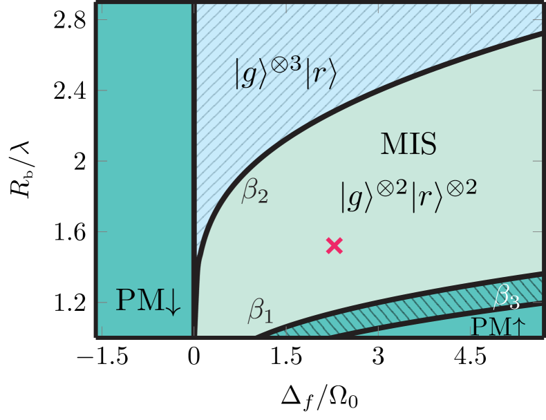
Figure 3: Phase diagram of $\mathds{P}_{4}$ graph showing the regions of dominant phases. Anti-ferromagnetic (A-F) phase where atoms singly excited to Rydberg state is bounded by $0<\Delta_{f}/\Omega_{0}\leq\beta_{2}(R_{\text{\tiny b}}/\lambda)$. MIS phase is dominant in the region $\beta_{1}(R_{\text{\tiny b}}/\lambda)<\Delta_{f}/\Omega_{0}<\beta_{2}(R_{\text{\tiny b}}/\lambda)$. There are two PM phases: (i) PM$\downarrow$ of ground states is bounded by $\Delta_{f}/\Omega_{0}<0$, and (ii) PM$\uparrow$ phase which is bounded by $\Delta_{f}/\Omega_{0}>\beta_{1}(R_{\text{\tiny b}}/\lambda)$. The phase bounded between $\beta_{1}(R_{\text{\tiny b}}/\lambda)<\Delta_{f}/\Omega_{0}<\beta_{3}(R_{\text{\tiny b}}/\lambda)$ is where three atoms can be excited to Rydberg state simultaneously.

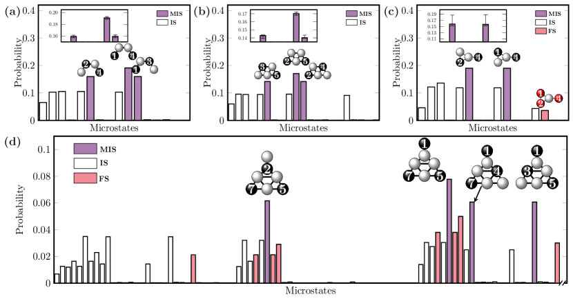
Figure 4: Probability distributions indicating the MIS solutions (violet bars) of the corresponding graphs in Fig. 1(a) for $\Delta_{\ell}/2\pi=-6.0$ $\mathrm{M}\mathrm{H}\mathrm{z}$, $\Delta_{f}/2\pi=4.0$ $\mathrm{M}\mathrm{H}\mathrm{z}$, $\tau=5.0$ $\mu\mathrm{s}$, and the graph spacing constant $\lambda=6.0$ $\mu\mathrm{m}$. The insets are showing the errors bars resulting from considering positional (radial and axial) fluctuations, $\delta_{\text{\tiny R}}=\pm 0.447$ $\mu\mathrm{m}$ ($\delta_{\text{\tiny x}}=\delta_{\text{\tiny y}}=0.1$ $\mu\mathrm{m}$), and $\delta_{\text{\tiny z}}=\pm 0.6$ $\mu\mathrm{m}$. White (red) bars correspond to the independent sets (frustrated sets). In (c), we have shown only the first 90 states of total $2^{7}=128$ states. The probabilities of other states are infinitely small.

IV Planar Graphs

IV.1 Maximum Independent Set (MIS)

The maximum indepenent sets of of unweighted planar graphs are obtained for the maximum Rydberg detuning $\Delta_{f}$ equal for all atoms resembling the graph, as shown in Fig. 1(a). Here we omit the weights of the vertices. The graph spacing constant $\lambda$ defines the distance between vertex $i$ and the nearest vertex $j$ ($i\neq j$) and is an alternative to the lattice constant $a$, which is shown in Fig. 1(d).

The phases of $\mathds{P}_{4}$ graph, shown in Fig. 1(a), could be different from the phases of an 1D atomic array due to differences in the energies of all pairwise interactions in a two-dimensional graph. In Fig. 3 the phase diagram of $\mathds{P}_{4}$ graph shows regions of dominant phases. The phase diagram is obtained by parameterizing the Hamiltonian via the ratios $R_{b}/\lambda$ and $\Delta_{f}/\Omega_{0}$. The positions of graph vertices are given in Table 1 as a function of the graph spacing constant $\lambda$. Fluctuations of positions of atoms, laser noise, and spontaneous emissions are neglected. The boundaries between different phases can be fitted by functions $\beta_{i}(\frac{R_{b}}{\lambda})=\frac{1}{4}\mathcal{C}_{6}^{\text{\scalebox{0.7}{Rb-Rb}}}e^{-\xi_{i}\frac{R_{b}}{\lambda}}$ where the parameters $\xi_{1}=1.4$, $\xi_{2}=2.8$, and $\xi_{3}=1.23$ define three different curves $\beta_{1}$, $\beta_{2}$, $\beta_{3}$, shown in Fig. 3. There are two different regions where paramagnetic phases (PM) are dominant: (i) PM$\downarrow$ phase is located where $\Delta_{f}<0$ and only the ground state of all four atoms $|g\rangle^{\otimes 4}$ can be found in this region of parameters. (ii) PM$\uparrow$ phase is located for $\Delta_{f}/\Omega_{0}>\beta_{3}$, where all atoms are excited to Rydberg state. The bounded phase between $\beta_{3}\leq\Delta_{f}/\Omega_{0}\leq\beta_{1}$ is PM$\uparrow$-like phase where three atoms can be excited to Rydberg state. For $0<\Delta_{f}/\Omega_{0}\leq\beta_{2}$, we observe a phase with only one atom excited to Rydberg state due to strong interaction between atoms. The state of the system in this phase can be written as $|\psi\rangle=\sum_{l\neq i,j,k}^{N}|g\rangle^{\otimes 3}_{i,j,k}|r\rangle_{l}$. The region, bounded between $\beta_{1}$ and $\beta_{2}$, is an anti-ferromagnetic phase revealing the MISs.

In Fig. 4, we show the calculated probability distributions of all possible states of an atomic system after being driven to the many-body ground state. We set the values of graph spacing constant $\lambda=7.0$ $\mu\mathrm{m}$ and the maximum value of Rydberg detuning $\Delta_{f}/\Omega_{0}=2.28$, which are compromised values for finding MISs as pointed out in Fig. 3. These values of $\lambda$ and $\Delta_{f}$ will be constant for all graphs in Fig. 4. We considered finite lifetimes of intermediate excited and Rydberg states using Lindblad equation, and performed a Monte-Carlo simulation to take into account fluctuations of atomic positions.

MISs of $\mathds{P}_{4}$ graph are {{1,3}, {1,4}, {2,4}}. These states are shown in Fig. 4(a) as positions of Rydberg atoms, i.e. state {1,3} corresponds to 1^st and 3^rd atoms excited into Rydberg states. Their probabilities are represented by violet bars. From Fig. 4(a) we can see that the quantum states corresponding to solutions of MIS demonstrate the highest probabilities. Finding the MISs of unit-disk graphs is a geometry-constrained problem, and the probabilities of MISs can be varied by adjusting the distance between vertices according to the phase diagram. The MISs of 3-Fan graph, shown in Fig. 4(b), are the same as in $\mathds{P}_{4}$ graph, since the vertex 1 is connected to all other vertices. However, the probabilities of MISs in 3-Fan graph are lower than the corresponding probabilities of MISs in $\mathds{P}_{4}$ graph. The sets {1,3}, and {2,4} of $\mathds{P}_{4}$ and {2,4} and {3,5} of 3-Fan graph are of the same geometric pattern and consequently have the same probabilities. The error bars in the inset show the range of calculated errors for the MISs states (plotted in the same sequence as in the main figure) due to the fluctuations of the atomic positions. The white bars show the probability of a single atom being excited to Rydberg state which corresponds to an independent set of the graph.

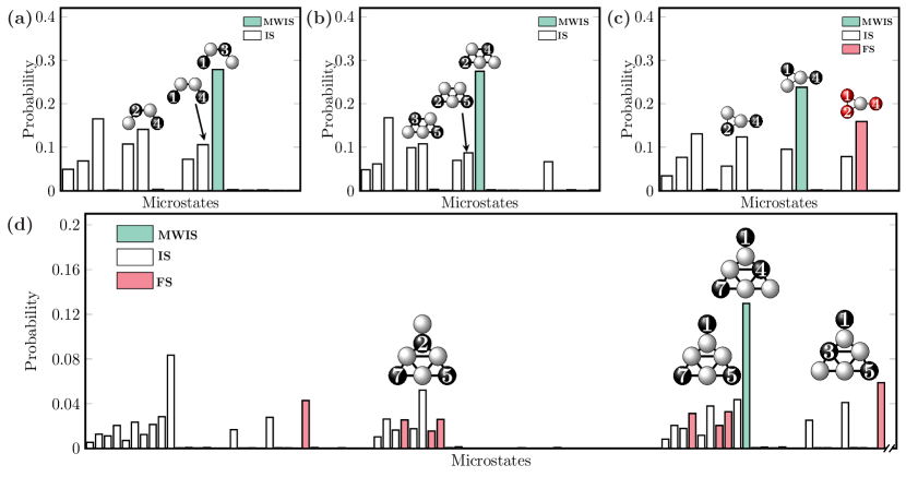
Figure 5: Probability distributions indicating the MWIS solutions (green bars) of the corresponding graphs in Fig. 1(a) with the same values of parameters, as in Fig. 4, but with different values of $\Delta_{f}$ [see the main text]. White (red) bars correspond to the independent sets (frustrated sets).

MISs of 3-Pan graph, shown in Fig. 4(c), are {{1,4}, {2,4}}. The corresponding states have almost equal probabilities, since both vertices 1and 2 are equally displaced from vertex 4. Also, the frustrated set/configuration {1,2,4} has appeared in the calculations due to imperfect Rydberg blockade for vertices 1 and 2.

Figure 4(d), shows the MISs of Eiffel tower graph [shown in Fig. 1(a)], which can be considered as combination of 3-Pan and 3-Fan graphs. MISs of tower graph are {{1,5,7}, {1,3,5}, {1,4,7}, {2,5,7}}. Frustrated configurations are also present, but they have smaller probabilities than MISs. The MISs {{1,3,5},{1,4,7}} have identical geometric pattern, and their probabilities are almost equal.

IV.2 Maximum-weight independent set (MWIS)

In this subsection, we study MWIS of the same graphs, which are shown in Fig. 1(a), but taking into account the weights of their vertices. The positions of the vertices and weights are defined in Table 1 and the weights are indicated in Fig. 1. The goal of MWIS is to find the independent set with the maximum sum of its weights. The weight of each vertex is represented by the maximum value of Rydberg detuning $\Delta_{f}$ [26]. The weights $\Delta_{f}$ of vertices are not equal. Therefore, the probability of exciting the particular atom to Rydberg state is different. In Fig. 5, we show the calculated probabilities of transition of the atomic ensemble from the ground state $|g\rangle^{\otimes\tiny\text{N}}$ to many-body states with different configuration of Rydberg excitations. In Fig. 5(a), the MWIS of $\mathds{P}_{4}$ graph is the set {1,3} which has much higher probability than other independent sets. Also, it can be noted that the probability of state {2,4} is higher than for {1,4}, which is different from the results in Fig. 4(a) for the MIS problem. Analogous results are obtained in Fig. 5(b). The MWIS for 3-Pan graph in Fig. 5(c) is {1,4}. It worth noting that the calculated probability for the frustrated set {1,2,4} is much higher than obtained before for the MIS problem for the same graph in Fig.4(c).

Overall, it is noted here that MWIS problem is not only a geometry-constrained as in the MIS. The probabilities of independent sets with the same geometric pattern, are not equal. Also, the probabilities of the MISs are sorted in ascending order of the sum of their weights .

V Non-planar graph

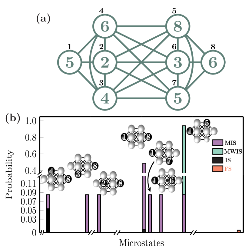
Figure 6: (a) The scheme of Johnson solid $J_{14}$ graph in 2D representation. The black label is the vertex number and the green one represent the weight of each vertex. The exact positions of vertices are given in Table 1. (b)The probabilities of MWISs for $J_{14}$. Some of graph states with infinitely small probabilities are omitted from the plotting.

In this section we discuss the results of finding the MWIS/MIS of a non-planar graph. Figure 6(a) shows a 2D scheme representation of $J_{14}$ graph. $J_{14}$ is a graph with 8 vertices in three dimensions, as defined in Table 1. $J_{14}$ is known as elongated equilateral triangular bipyramid, which is one of Johnson 92 convex polyhedra solids [55], whose facets are regular polygons. The graph includes $\mathcal{F}=9$ faces, as $6$ equilateral triangles, and $3$ squares. Euler’s characteristic of this graph is $\chi=V-E+\mathcal{F}=2$. A similar non-planar graph, represented in 2D, is called $\bar{X}_{152}$ as classified in the nomenclature of the Information System on Graph Classes and their Inclusions (ISGCI). $J_{14}$ graph is a combination of two 3-Pan graphs.

In Fig. 6(b), we plot the calculated probabilities of MISs and MWISs for $J_{14}$ graph in two cases. (i) All vertices are equally weighted, which shows the MISs {{1,5}, {1,6}, {1,7}, {1,8}, {2,8}, {3,8}, {4,8}} in violet-colored bars of Fig. 6(b). The sets {{1,5}, {1,6}, {1,7}, {2,8}, {3,8}, {4,8}} have obtained the same probability due to the fact that the atoms, representing vertices, are physically displaced equally from each other. Frustrated sets can be obtained from the simulation with probabilities much smaller than MISs. (ii) The weights of vertices are not equal [weight of each vertex is green-labeled in Fig. 6(a)]. The MWIS according to the considered weights is {1,5} as shown by a green-bar of Fig. 6(b). The independent sets, when considering the weighted graph, are the over plotted black-colored bars. The frustrated set {1,2,…,8} ($|r\rangle^{\otimes 8}$) is shown in the red bar and exhibits infinitely low probability.

VI Quantum Wire

In this section, we consider mediating strong interaction between far-distant vertices using the concept of quantum wire [56, 4]. Here we consider a quantum wire consisting of atoms of different chemical element. This allows separation of the readout wavelengths during detection of MIS/MWIS and suppression of crosstalk between neighboring atoms. Heteronuclear Rydberg interaction in the atomic arrays was first discussed in Ref. [39]. The concept of heteronuclear quantum annealers was then introduced in Ref. [6]. A dual-element heteronuclear Rb-Cs array of ultracold atoms was experimentally demonstrated in Ref. [57]. Schemes of CNOT gates with several control and target atoms exploiting heteronuclear Rydberg interactions were studied in Ref. [38]. The two-qubit CZ gate with different chemical elements was demonstrated in Ref. [58], showing advantages compared with homonuclear architectures. The scalability of heteronuclear atomic architecture with coherent transport of control qubits was studied in Ref. [59]. Analysis of heteronuclear interspecies interactions between Rydberg $d$-states of Rb and Cs atoms was presented in Ref. [60]. Dual-species model of quantum processors with single atoms or superatoms in the regime of Rydberg blockade was developed for quantum computations without the need of local addressing [61]. Here we propose using a quantum wire of Cs atoms created from array of traps generated by acousto-optic deflector, while the graph is represented by Rb atoms, which are loaded in the array of static traps generated by spatial light modulator. The ground state of Cs atoms of the quantum wire $|g\rangle_{\text{\tiny W}}=|6S_{1/2},F=3,m_{F}=3\rangle$ are excited to Rydberg state $|r\rangle_{\text{\tiny W}}=|81S_{1/2},m_{j}=1/2\rangle$ through the intermediate state $|m\rangle_{\text{\tiny W}}=|7P_{3/2},F=2\rangle$ by using $460$ $\mathrm{n}\mathrm{m}$ and $1039$ $\mathrm{n}\mathrm{m}$ laser lights, respectively. Atoms representing the graph and the wire are excited to the Rydberg state with the same principal quantum number $n=81$. In this case the dominant regime of interaction is van der Waals [36]. Figures 7(a, b) show the interaction between pairs of Rb and Cs atoms (graph and wire), and pairs of Cs atoms (wire-wire), respectively. For interatomic distance $R>R_{\text{\tiny vdW }}\simeq 4$ $\mu\mathrm{m}$, it is guaranteed that all interactions are in vdW regime. The values of $\mathcal{C}_{3}$ and $\mathcal{C}_{6}$ for all interactions are calculated by fitting the curves with the calculated interaction energy with all parameters as in Fig. 2(b). The quantum wire should be in the anti-ferromagnetic phase, where at most only one of the adjacent atoms can be excited to Rydberg state, known as $\mathds{Z}_{2}$-phase.

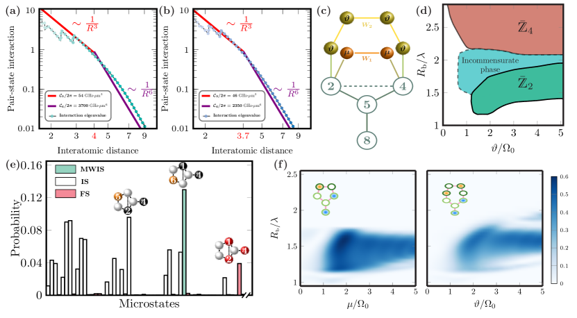
Figure 7: (a) The pair-state energy ($\mathrm{G}\mathrm{H}\mathrm{z}$) for the heteronuclear interaction between Rb and Cs atoms excited simultaneously to Rydberg state $|81S_{1/2},m_{j}=1/2\rangle$ considering the same conditions and methods in Fig. 1(c). (b) The pair-state energy interaction energy between two Cs atoms. (c) The graph scheme of 3-Pan graph with vertices 1 and 2 are connected using two different spatial configurations of quantum wires $W_{1}$ (two vertices in violet color) and $W_{2}$ (four vertices in orange color). (d) The phase diagram of mediating the vertices $\text{v}_{1}$, $\text{v}_{2}$ by the quantum wire $W_{2}$ composed of two equally weighted vertices $\text{v}_{5}$ and $\text{v}_{6}$ (weight $\mu$ $\mathrm{M}\mathrm{H}\mathrm{z}$). The quantum wire $W_{1}$ is in the anti-ferromagnetic phase in the region bounded by $\zeta_{2}(R_{b}/\lambda)$, and $\zeta_{3}(R_{b}/\lambda)$. (e) The probabilities indicating the MWIS of 5-Pan graph (3-Pan+$W_{1}$). (f) The contour plots of the MWIS of 5-Pan (left panel) and 7-Pan (right panel) graphs as a function of wire weights $\Delta_{f}=\mu$ ($\mathrm{M}\mathrm{H}\mathrm{z}$) and graph spacing constant $\lambda$ ($\mu\mathrm{m}$).

Figure 7(c) illustrates mediation of interaction between the vertices $\text{v}_{1}$ and $\text{v}_{2}$ of a 3-Pan graph by two quantum wires ($W_{1}$ and $W_{2}$) formed of Cs atoms. The quantum wires are of different lengths (have different number of atoms) $\bar{w}_{1}=2$, and $\bar{w}_{2}=4$ . Atoms of each wire are equally weighted. The weights of quantum wire $W_{1}$ are $\mu/2\pi$ and for $W_{2}$ are $\vartheta/2\pi$.

In Fig. 7(d), we plot the phase diagram of a 3-Pan graph with quantum wire $W_{2}$ showing the probabilities as a function of two dimensionless parameters: the ratio of wire weights to the effective Rabi frequency $W_{2}/\Omega_{0}$, and the ratio of Rydberg blockade radius to the graph spacing constant $R_{b}/\lambda$ . If the quantum wire $W_{2}$, consisting of four atoms, is not connected to graph atoms, then the probability distribution of its quantum states for the same laser excitation pattern, as shown in Fig. 2(b) should behave similarly to the phase diagram, shown in Fig. 3. The phase diagram in Fig. 7(d) shows the realization of different ordered state $\bar{\mathds{Z}}_{2}$ [the bar sign over $\mathds{Z}_{2}$ indicates that the ordered states for a graph are different from the linear configuration from Fig. 1(d)]. The ordered state $\bar{\mathds{Z}}_{4}$ is also realized for the graph-wire states $|gggr\rangle_{\text{G}}|gggr\rangle_{\text{W}_{2}}$ and $|gggr\rangle_{\text{G}}|ggrg\rangle_{\text{W}_{2}}$.

Figure 8: The probability distribution of the incommensurate state $|rggr\rangle_{\text{G}}|gggr\rangle_{\text{W}_{2}}$

In Fig. 7(e), we show the probabilities of finding the MWIS ({1,4}=$|rggr\rangle_{G}|gr\rangle_{W_{1}}$) of 3-Pan graph while using the quantum wire $W_{1}$ to mediate the interaction between $\text{v}_{1}$ and $\text{v}_{2}$. Finding MWIS {1,4} of 3-Pan graph is independent of the wire weights $\mu$ as shown in Fig. 7(f), and the MWIS is {1,4,6} (the bold text indicating the excited wire atom to Rydberg state). In Fig. 7(f), we plot the probabilities of states $\{1,4,6\}=|rggr\rangle_{\scalebox{0.6}{G}}|gr\rangle_{\scalebox{0.6}{W}_{1}}$ and $\{1,4,6,7\}=|rggr\rangle_{\scalebox{0.6}{G}}|grrg\rangle_{\scalebox{0.6}{W}_{2}}$ in the left and right panels, respectively. The contour plot shows the probability of the considered state as a function of the weights of the wire atoms and distance parameter $\lambda$. In this figure we illustrate the effect of using quantum wires of different lengths (numbers of atoms). As shown, the minimum value of vertices weight to get the probability of the MWIS with a quantum wire $W_{1}$ formed of two auxiliary atoms is $\mu/\Omega_{0}\simeq 0.92$, while for a quantum wire $W_{2}$ formed of four auxiliary atoms $\vartheta/\Omega_{0}\simeq 1.2$.

Due to the spatial arrangement of atoms representing the graph, an incommensurate phase emerges, showing a combination of $\bar{\mathds{Z}}_{2}$ and $\bar{\mathds{Z}}_{3}$ ordered states. The probability distribution of the incommensurate state is shown in Fig. 8. The realization of this incommensurate phase is controlled by the Rydberg detuning of each atom of the considered array in 2D spatial arrangement of the atoms. This phase may boost realizing new dimer models which can be obtained from optimizing the interaction between atoms of homonuclear or heteronuclear architecture with the detuning of Rydberg state of each atom. In Fig. 7(f), the length of the quantum wire changes the dynamics of the system. In this case the quantum wire is not in anti-ferromagnetic phase and that breaks the considered condition [4], then the quantum wire $W_{2}$ can be regarded as superatom [61].

VII Conclusion

We considered solution of MIS and MWIS problems using arrays of ultracold neutral atoms excited to Rydberg states using a non-linear quasi-adiabatic time profile of detuning from the two-photon resonance with Rydberg states. We have obtained MISs and MWIS of planar and non-planar graphs. For MIS problem, we have concluded that it is a geometry constrained problem, and generation of the independent sets for same geometric patterns have equal probabilities. For the MWIS problem the weights of each vertex change the character of the resulting most probable independent set. The use of quantum wire can help mediating strong interactions of far-distant vertices. Also, quantum wires can be used to perform quantum annealing of non unit-disk graphs. Using heteronuclear structure of the atomic array it is feasible to distinguish the measurement of atomic states representing the graph and the wire vertices due to the separation of the wavelengths and reduction of cross-talk among different chemical elements. Moreover, the cost ($\Delta_{f}$) of finding the MIS or MWIS increases proportionally for longer lengths of quantum wires.

We studied the quantum phase transitions from disordered to ordered-crystalline states of 1D atomic array, and realized $\mathds{Z}_{2}$ and $\mathds{Z}_{3}$ ordered states with the existence of a domain wall in $\mathds{Z}_{2}$. Also, an incommensurate floating phase between $\mathds{Z}_{3}$ and $\mathds{Z}_{4}$ is obtained. An incommensurate floating phase between $\bar{\mathds{Z}}_{2}$ and $\bar{\mathds{Z}}_{3}$ in 2D atomic array, formed as 7-Pan graph representation, is realized allowing to use quantum wire, which is not in anti-ferromagnetic state, for solving MWIS. This incommensurate phase does not exist in 1D arrays for equal detunings of transitions to Rydberg state. The results of incommensurate phases can open new directions for realizing exotic states of matter.

Note added: During the completion of this manuscript we became aware of the foremost experimental demonstration of the weighted graphs, verifying the ability to prepare weighted graphs in 1D and 2D arrays [63].

Table 1: Sites of atoms demonstrating the considered graphs as a function of graph spacing constant $\lambda$.

Graph	Positions
$\mathds{P}_{4}$	1:$\left(-\lambda,0,0\right)$, 2: $\left(-\frac{1}{2}\lambda,\frac{\sqrt{3}}{2}\lambda,0\right)$, 3: $\left(\frac{1}{2}\lambda,\frac{\sqrt{3}}{2}\lambda,0\right)$,       4:$\left(\lambda,0,0\right)$
$\left[~{}\text{Fig.}~{}\ref{Fig:SysDynamics}(a)~{}\right]$
3-Fan	1:$\left(0,0,0\right)$,    2:$\left(-\lambda,0,0\right)$,            3: $\left(-\frac{1}{2}\lambda,\frac{\sqrt{3}}{2}\lambda,0\right)$,    4: $\left(\frac{1}{2}\lambda,\frac{\sqrt{3}}{2}\lambda,0\right)$,
$\left[~{}\text{Fig.}~{}\ref{Fig:SysDynamics}(a)~{}\right]$	5:$\left(\lambda,0,0\right)$.
3-Pan	1: ($\frac{-\lambda}{\sqrt{2}}$, $\frac{\lambda}{\sqrt{2}}$, 0.0), 2: ($\frac{-\lambda}{\sqrt{2}}$, $\frac{-\lambda}{\sqrt{2}}$, 0.0), 3: (0.0, 0.0, 0.0),  4: ($\lambda$, 0.0, 0.0).
$\left[~{}\text{Fig.}~{}\ref{Fig:SysDynamics}(a)~{}\right]$
———	——————————————————
5-Pan ($\textbf{W}_{1}$)	5: $\left(-\frac{1}{\sqrt{2}}\lambda-\frac{1}{2}\lambda\sqrt{1+2\sqrt{2}},\frac{1}{2}\lambda,0.0\right)$   6: $\left(-\frac{1}{\sqrt{2}}\lambda-\frac{1}{2}\lambda\sqrt{1+2\sqrt{2}},-\frac{1}{2}\lambda,0.0\right)$
$\left[~{}\text{Fig.}~{}\ref{Fig:QWire}(c)~{}\right]$
———	——————————————————
7-Pan ($\textbf{W}_{2}$)	5: $\left(-\frac{1}{\sqrt{2}}\lambda-\lambda,\frac{1}{\sqrt{2}}\lambda,0.0\right)$                       6: $\left(-\frac{1}{\sqrt{2}}\lambda-\lambda,-\frac{1}{\sqrt{2}}\lambda,0.0\right)$
$\left[~{}\text{Fig.}~{}\ref{Fig:QWire}(c)~{}\right]$	7: $\left(-\frac{1}{\sqrt{2}}\lambda-\lambda-\frac{1}{2}\lambda\sqrt{1+2\sqrt{2}},\frac{1}{2}\lambda,0.0\right)$    8: $\left(-\frac{1}{\sqrt{2}}\lambda-\lambda-\frac{1}{2}\lambda\sqrt{1+2\sqrt{2}},-\frac{1}{2}\lambda,0.0\right)$
Tower	1: (0.0, 0.0, 0.0),          2: (0.0, $-\lambda$, 0.0),              3: ($\frac{-\lambda}{\sqrt{2}}$,  $\frac{-\lambda}{\sqrt{2}}-\lambda$, 0.0),
$\left[~{}\text{Fig.}~{}\ref{Fig:SysDynamics}(a)~{}\right]$	4: ($\frac{\lambda}{\sqrt{2}}$, $\frac{-\lambda}{\sqrt{2}}-\lambda$, 0.0),     5: ($\frac{2\lambda}{\sqrt{2}}$, $\frac{-2\lambda}{\sqrt{2}}-\lambda$, 0.0),       6: (0.0, $-\lambda(1+\sqrt{2})$, 0.0),
	7: ($\frac{-2\lambda}{\sqrt{2}}$, $\frac{-2\lambda}{\sqrt{2}}-\lambda$, 0.0).
$J_{14}$	1: $\left(x_{0},y_{0},\eta_{0}\lambda\right)$,                       2: $\left(x_{0},y_{0}+\frac{\lambda}{\sqrt{3}},-\lambda\right)$,                    3: $\left(x_{0}-\frac{\lambda}{2},y_{0}-\frac{\lambda}{2\sqrt{3}},-\lambda\right)$,
$\left[~{}\text{Fig.}~{}\ref{Fig:JohnsonGraphJ14}~{}\right]$	4: $\left(x_{0}+\frac{\lambda}{2},y_{0}-\frac{\lambda}{2\sqrt{3}},-\lambda\right)$,        5: $\left(x_{0}+\frac{\lambda}{2},y_{0}-\frac{\lambda}{2\sqrt{3}},-2\lambda*q_{0}\right)$,     6: $\left(x_{0},y_{0}+\frac{\lambda}{\sqrt{3}},-2\lambda*q_{0}\right)$,
	7: $\left(x_{0}-\frac{\lambda}{2},y_{0}-\frac{\lambda}{2\sqrt{3}},-2\lambda*q_{0}\right)$, 8: $\left(x_{0},y_{0},-\lambda(\eta_{0}+2q_{0}+1)\right)$.
	where $x_{0}$, and $y_{0}$ are arbitrary points. In calculatioons, we considered $x_{0}=y_{0}=0$.
	To get equal lengths of triangle and square sides, we set $\eta_{0}\simeq-0.183368$, and $q_{0}=1$.