Generalized Holographic Reduced Representations

Abstract

Deep learning has achieved remarkable success in recent years. Central to its success is its ability to learn representations that preserve task-relevant structure. However, massive energy, compute, and data costs are required to learn general representations. This paper explores Hyperdimensional Computing (HDC), a computationally and data-efficient brain-inspired alternative. HDC acts as a bridge between connectionist and symbolic approaches to artificial intelligence (AI), allowing explicit specification of representational structure as in symbolic approaches while retaining the flexibility of connectionist approaches. However, HDC’s simplicity poses challenges for encoding complex compositional structures, especially in its binding operation. To address this, we propose Generalized Holographic Reduced Representations (GHRR), an extension of Fourier Holographic Reduced Representations (FHRR), a specific HDC implementation. GHRR introduces a flexible, non-commutative binding operation, enabling improved encoding of complex data structures while preserving HDC’s desirable properties of robustness and transparency. In this work, we introduce the GHRR framework, prove its theoretical properties and its adherence to HDC properties, explore its kernel and binding characteristics, and perform empirical experiments showcasing its flexible non-commutativity, enhanced decoding accuracy for compositional structures, and improved memorization capacity compared to FHRR.

1 Introduction

In the past decade of artificial intelligence research, deep learning has seen monumental success, finding applications in domains such as classification, image generation, and language modeling [1, 2, 3, 4, 5]. Central to the success of deep learning is its ability to learn representations that preserve task-relevant structure in the data, a necessary component for models with generalization capabilities. Indeed, this reliance on the quality of representations is reflected in the common use of pre-trained models, and, more recently, in foundation models [6].

However, underpinning deep learning models with good representations are tremendous computational resources and internet-scale data in the order of terabytes and beyond. While research into scaling laws suggests that it is possible to further improve the model and thus representation quality by continuing to scale up model size, data quantity, and computational resources [7], this approach is extremely cost-inefficient, time-consuming, and excludes all but the largest and most resourceful organizations from the development of such models.

Thus, it is necessary to explore directions that are compute- and data-efficient while having representational properties amenable to generalization. For this purpose, we turn to the brain for inspiration.

In recent years, Hyperdimensional Computing (HDC), or Vector Symbolic Architectures (VSA), has emerged as a brain-inspired computational paradigm in artificial intelligence bridging the gap between connectionist and symbolic frameworks [8, 9]. In this way, HDC can act as an interface that enables the explicit specification of structure as in symbolic approaches while maintaining the flexibility and power of connectionist, especially deep learning, approaches. HDC forms an algebra over higher-dimensional vectors, called hypervectors, with operations corresponding to cognitive operations. For example, the bundling operation corresponds to memorization and binding corresponds to association. This is a powerful idea in the context of neural representations, as through the use of such operations, it is possible to build up complex representations and data structures [10, 11, 12, 13], and consequently instill a factorized structure onto the space of representations, which can subsequently be used in downstream tasks such as symbolic reasoning [14, 15].

While HDC shows promise as a neuro-vector-symbolic framework for factorized and compositional representations, its simplicity poses a problem for its expressive power and its ability to encode more complex structures. In particular, crucial to the HDC framework is the binding operation, which enables the formation of representational complexes from simpler parts, often interpreted as an association or conjunction of concepts. This, however, is limiting, as concepts may hold various kinds of relationships with each other and may be combined in multiple ways. In addition, implementations of binding in HDC are typically commutative, so additional techniques such as applying permutations or positional encodings are often needed to encode structure, which complicates the representation of data structures. Thus, we need a more flexible and non-commutative binding operation more suitable for encoding complex structures, while still maintaining the other desirable properties of HDC, such as transparency, robustness to noise, and interpretability.

In this paper, we introduce Generalized Holographic Reduced Representations (GHRR), an extension of Fourier Holographic Reduced Representations (FHRR) [16, 17], which is a particular implementation of HDC. While maintaining the kernel properties of FHRR [18] and satisfying the basic constraints of HDC representations, GHRR provides a framework for flexible, non-commutative binding as well as adaptive kernels while enabling improved encoding of complex data structures via better decoding abilities and memorization of bound hypervectors. Our work has several key contributions:

1. We introduce the GHRR framework and outline a particular implementation of GHRR, including variations of increasing complexity.

2. We prove that our implementation of GHRR satisfies the basic properties of HDC, including quasi-orthogonality and that the similarity preservation of the binding operation.

3. We explore the kernel and binding properties of GHRR and provide an interpretation of binding in GHRR as an interpolation between binding in FHRR and in Tensor Product Representations [19].

4. We perform empirical experiments on GHRR, demonstrating its flexible non-commutativity, increased decoding accuracy for compositional structures e.g. trees, and improved memorization capacity for bound hypervectors compared to FHRR.

2 Background

2.1 Hyperdimensional Computing Basics

Hyperdimensional Computing (HDC), also known as Vector Symbolic Architecture (VSA), is a computing framework inspired by the brain. It is motivated by the observation that representations in the brain are high-dimensional, consisting of neural activations of a large population of neurons [8]. Moreover, while these population-level representations appear to be highly distributed and stochastic across different brains, they exhibit the same cognitive properties at a high level [20, 21].

The fundamental unit in HDC is a high dimensional vector, also called a hypervector, corresponding to the population-level neural activations. A hypervector $H$ lives in some hyperspace $H$, e.g., $\mathbb{R}^{D}$ for $D$ large. The collection of hypervectors, along with some operators, forms an algebra over vectors. Generally, there are two types of hypervectors: (1) base hypervectors, which are generated stochastically, e.g., $H\sim\mathcal{N}(0,I)$; and (2) composite hypervectors, which are created by combining hypervectors via the operators of the algebra. These hypervectors can be compared via a similarity function $\delta(H_{1},H_{2})$. Generally, base hypervectors are generated such that they are quasi-orthogonal with respect to the similarity function. The three main operations in HDC, bundling, binding, and permutation, can be characterized by how they affect the similarity of hypervectors. We describe the three operations below:

1. Bundling ($+$): Typically implemented as element-wise addition. If $H=H_{1}+H_{2}$, then both $H_{1}$ and $H_{2}$ are similar to $\mathcal{H}$. From a cognitive perspective, it can be interpreted as memorization.

2. Binding ($*$): Typically implemented as element-wise multiplication. If $H=H_{1}*H_{2}$, then $H$ is dissimilar to both $H_{1}$ and $H_{2}$. Binding also has the important property of similarity preservation in the sense that for some hypervector $H_{3}$, $\delta(H_{3}*H_{1},H_{3}*H_{2})\simeq\delta(H_{1},H_{2})$. From a cognitive perspective, it can be interpreted as the association of concepts.

3. Permutation ($\rho$): Typically implemented as a rotation of vector elements. Generally, $\delta(\rho(H),H)\simeq 0$. Permutation is usually used to encode order in sequences.

It is important to note that the description above of HDC is general; there are various specific realizations of HDC with the above properties.

The HDC framework gives several benefits, including robustness to noise in hyperspace, transparency, and parallelization.

2.2 Fourier Holographic Reduced Representations

Fourier Holographic Reduced Representations (FHRR) is a specific implementation of HDC. An FHRR hypervector is of the form $H=[e^{i\theta_{1}},...,e^{i\theta_{D}}]$. Bundling and binding are the usual element-wise addition and multiplication, respectively. In addition, the similarity is defined as $\delta(H_{1},H_{2}):=\mathfrak{R}[H_{1}^{\dagger}H_{2}]/D$, where $\dagger$ denotes the conjugate transpose.

Fractional power encoding (FPE) has been used for encoding data points to hypervectors. It is a locality-preserving encoding for points on a data manifold where the similarity, or inner product, of the hypervectors reflects the relationship between the points [22, 23]. For the $k^{th}$ feature of data of dimension $n$, attached is an FHRR base hypervector of the form $\mathcal{H}_{k}=e^{i\theta}$, where $\theta$ is a column vector such that $\theta_{j}\sim p_{k}$ for some fixed distribution $p_{k}$. The data point is then encoded as the binding of the base hypervector exponentiated by the value of the corresponding feature: $\phi(x)=\mathcal{H}_{1}^{x_{1}}*\mathcal{H}_{2}^{x_{2}}*...*\mathcal{H}_{n}^{x_{n}}$. This allows the data to be smoothly expressed and manipulated in the context of a data manifold.

An alternative formulation of the fractional power encoding may bring insight into why HDC models can learn effectively [24, 25, 23, 26, 27, 28, 29, 30, 31]. In particular, it coincides with the Random Fourier Features (RFF) [18] encoding, an efficient approximation of kernel methods. The RFF encoding is a map $\phi:\mathbb{R}^{n}\to\mathcal{C}^{D}$, with $\phi(x)=e^{iMx}$, where each row $M_{j,:}\sim p$ for some multivariate distribution $p$. The columns $M_{:,k}$ can then be viewed as the exponents of the base hypervector $\mathcal{H}_{k}$, and $p=[p_{1},...,p_{n}]$. As a result of Bochner’s theorem, $\langle\phi(x),\phi(y)\rangle/D\approx K(x-y)$, where $K$ is a shift-invariant kernel that is the Fourier transform of distribution $p$ [18]. Notably, when $p$ is the standard multivariate Gaussian distribution, the radial basis function (RBF) kernel is recovered. Many HDC learning models achieve good time and accuracy performance by the efficient kernel approximation coupled with some HDC algorithm.

3 Overview of GHRR

In this section, we provide the general framework for GHRR. We first observe that each component of an FHRR base hypervector is unitary; i.e. $e^{i\theta}\in\mathrm{U}(1)$. Thus, it is natural to want to extend each component to be a member of $\mathrm{U}(m)$ for $m\geq 1$. This is precisely what GHRR base hypervectors are. They are tensors of the form

$$H=[a_{1},...,a_{D}]^{\top}\in\mathbb{C}^{D\times m\times m},$$ (1)

where $a_{j}\in\mathrm{U}(m)$ such that $a_{j}\sim p$ for some distribution $p$ over $\mathrm{U}(m)$, for $j=1,...,D$.

The standard operations in HDC extend naturally. Let $H_{1}=[a_{j}]_{j=1}^{D}$ and $H_{2}=[b_{j}]_{j=1}^{D}$. We define bundling to be element-wise addition, i.e.

$$H_{1}+H_{2}=[a_{j}+b_{j}]_{j=1}^{D},$$ (2)

and binding to be element-wise matrix multiplication, i.e.

$$H_{1}*H_{2}=[a_{j}b_{j}]_{j=1}^{D}.$$ (3)

We define the similarity between two hypervectors as

$$\delta(H_{1},H_{2})=\frac{1}{mD}\mathfrak{R}\,\text{tr}\left(\sum_{j=1}^{D}a_{j}b_{j}^{\dagger}\right).$$ (4)

It can be seen that for $m=1$, this similarity is exactly that for FHRR. Note that after bundling, the matrix entries need not be unitary. However, we still require that base hypervectors be unitary such that they are similar to themselves under the similarity defined in Eq. 4. Figure 1 provides an overview of and comparison between GHRR and FHRR.

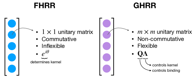
Figure 1: Comparison between FHRR and GHRR.

4 An Implementation of GHRR

What we have described in Section 3 are general characteristics of GHRR. Specifying an implementation entails specifying (1) the form of the unitary matrix components; and, relatedly, (2) how they are sampled.

4.1 Desired Properties

We want our GHRR representations to fulfill the basic properties of HD representations. Most notably, we need the binding operation for representing the association of features works as intended [32]. for different base hypervectors $H_{1},H_{2},H_{3}$,

1. $\delta(H_{1},H_{2})\to 0$ as $D\to\infty$; and

2. $\delta(H_{1}*H_{2},H_{1})\to 0$ as $D\to\infty$.

3. $\delta(H_{1},H_{2})\approx\delta(H_{3}*H_{1},H_{3}*H_{2})\approx\delta(H_{1}*H_{3},H_{2}*H_{3})$.

While property 3 follows naturally from the cyclic property of the trace, the other two properties do not hold in arbitrary implementations. In addition, since GHRR is an extension of FHRR, we want the two to be equivalent when $m=1$.

4.2 Quasi-orthogonal Representations

We derive sufficient conditions for these properties to hold, and based on that, develop a constrained parameterization for GHRR representations.

Proposition 4.1.

Let $\mathbf{A}=\mathbf{Q}_{1}\mathbf{\Lambda}_{1},\mathbf{B}=\mathbf{Q}_{2}\mathbf{\Lambda}_{2}\in\mathbb{C}^{m\times m}$ be random matrices where $\mathbf{Q}_{j},\mathbf{\Lambda}_{j}$ are sampled independently of each other for $j=1,2$. Moreover, let $\mathbf{\Lambda}_{1}=\mathrm{diag}(\lambda_{1},...,\lambda_{m})$ and $\mathbf{\Lambda}_{2}=\mathrm{diag}(\eta_{1},...,\eta_{m})$ with $\lambda_{j},\eta_{j}\in\mathrm{U}(1)$ for $j=1,...,m$. If $\mathbb{E}[\eta_{j}\lambda_{j}^{*}]=0$ for all $j=1,...,m$, then $\mathbb{E}\,\mathrm{tr}(\mathbf{AB^{\dagger}})=0$.

Proof.

Without loss of generality, let $\mathbf{A}=\mathbf{Q}\mathbf{\Lambda}_{1}$ and $\mathbf{B}=\mathbf{\Lambda_{2}}$, as by the cyclic property of the trace,

$$\mathrm{tr}(\mathbf{AB}^{\dagger}) =\mathrm{tr}(\mathbf{Q}_{1}\mathbf{\Lambda}_{1}\mathbf{\Lambda}_{2}^{\dagger}\mathbf{Q}_{2}^{\dagger})$$ (5)

$$=\mathrm{tr}((\mathbf{Q}_{2}^{\dagger}\mathbf{Q}_{1})\mathbf{\Lambda}_{1}\mathbf{\Lambda}_{2}^{\dagger}),$$ (6)

so we can set $\mathbf{Q}=\mathbf{Q}_{2}^{\dagger}\mathbf{Q}_{1}$. Simple algebraic manipulation gives us

$$\mathrm{tr}(\mathbf{AB}^{\dagger}) =\sum_{k=1}^{m}\lambda_{k}\eta_{k}^{*}\mathbf{Q}_{kk}.$$ (7)

Taking expectations, we get

$$\mathbb{E}\,\mathrm{tr}(\mathbf{AB}^{\dagger}) =\sum_{k=1}^{m}\mathbb{E}[\lambda_{k}\eta_{k}^{*}\mathbf{Q}_{kk}]$$ (8)

$$=\sum_{k=1}^{m}\mathbb{E}_{\mathbf{Q}}[\mathbb{E}_{\lambda,\eta|\mathbf{Q}}[\lambda_{k}\eta_{k}^{*}]\mathbf{Q}_{kk}]$$ (9)

$$=\sum_{k=1}^{m}\mathbb{E}_{\lambda,\eta}[\lambda_{k}\eta_{k}^{*}]\mathbb{E}_{\mathbf{Q}}[\mathbf{Q}_{kk}]=0.$$ (10)

∎

Corollary 4.1.1.

Suppose we sample random matrices $\mathbf{A},\mathbf{B}$ with the form $\mathbf{Q\Lambda}$, where $\mathbf{Q}\in\mathbb{C}^{m\times m}$ is a randomly sampled unitary matrix and, independently, $\mathbf{\Lambda}=\mathrm{diag}(\lambda_{1},...,\lambda_{m})$, where $\lambda_{j}\sim p_{j}$ where $p_{j}$ is a symmetric distribution with zero mean for $j=1,...,m$. Then $\mathbb{E}\,\mathrm{tr}(\mathbf{AB}^{\dagger})=0$.

Corollary 4.1.2.

Suppose we sample random matrices $\mathbf{A},\mathbf{B}$ according to Corollary 4.1.1. Then $\mathbb{E}\,\mathrm{tr}(\mathbf{A}(\mathbf{AB})^{\dagger})=0$.

Proof.

Observe that

$$\mathbb{E}\,\mathrm{tr}(\mathbf{A}(\mathbf{AB})^{\dagger}) =\mathbb{E}\,\mathrm{tr}(\mathbf{A}\mathbf{B}^{\dagger}\mathbf{A}^{\dagger})=\mathbb{E}\,\mathrm{tr}(\mathbf{I}\mathbf{B}^{\dagger}).$$ (11)

Since $\mathbf{B}=\mathbf{Q\Lambda}$ where $\mathbf{\Lambda}=\mathrm{diag}(\lambda_{1},...,\lambda_{m})$, with $\lambda_{j}$ sampled from distributions with zero mean, $\mathbb{E}\,\lambda_{j}=0$ for all $j=1,...,m$. So Proposition 4.1 applies and we are done. ∎

Corollary 4.1.1 gives us a way to construct base hypervectors satisfying the desiderata mentioned above. By default, Corollary 4.1.1 gives us desired property 1, while Corollary 4.1.2 gives us desired property 2. Moreover, it is evident that when $m=1$, this GHRR implementation is equivalent to FHRR. Thus, a GHRR base hypervector is of the form

$$[\mathbf{Q}_{1}\mathbf{\Lambda}_{1},...,\mathbf{Q}_{D}\mathbf{\Lambda}_{D}]^{\top},$$ (12)

where $\mathbf{Q}_{j}\in U(m)$ and $\mathbf{\Lambda}_{j}=\mathrm{diag}(e^{i\theta_{1}},...,e^{i\theta_{m}})$, with $\theta_{k}\sim p_{k}$ such that $\mathbb{E}[e^{i\theta_{k}}]=0$. Figure 2 shows a histogram of the similarity between randomly sampled hypervectors following the scheme described in Corollary 4.1.1, where $D=1000$, $m=3$, and $p_{j}=\mathrm{Unif}(0,2\pi)$. We observe that the randomly sampled hypervectors are quasi-orthogonal; i.e. their similarities are concentrated about zero. The top histogram holds $\mathbf{Q}_{j}=\mathbf{Q}_{k}$ for all $j,k=1,...,D$, while the middle histogram has randomly sampled $\mathbf{Q}_{j}$. The bottom histogram shows that the similarity between $H_{1}$ and $H_{1}*H_{2}$ respects the result in Corollary 4.1.2.

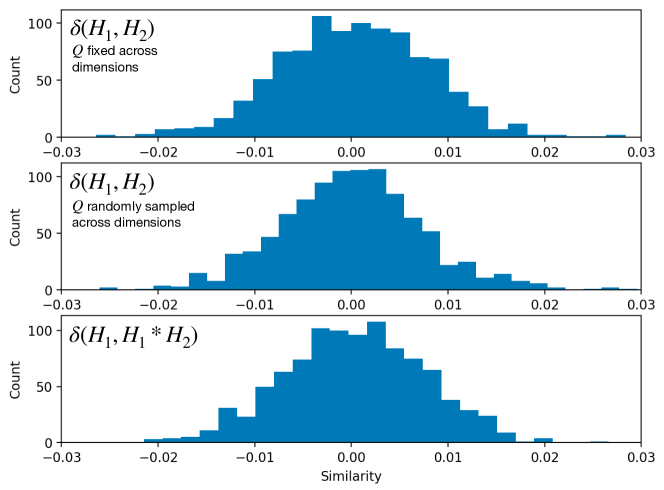
Figure 2: A histogram of the similarity between randomly sampled hypervectors following the scheme described in Corollary 4.1.1, where $D=1000$, $m=3$, and $p_{j}=\mathrm{Unif}(0,2\pi)$. Top: Histogram where $\mathbf{Q}_{j}=\mathbf{Q}_{k}$ holds for all $j,k=1,...,D$. Middle: histogram where $\mathbf{Q}_{j}$ for $j=1,...,D$ are randomly sampled. Bottom: histogram of similarity between $H_{1}$ and $H_{1}*H_{2}$.

4.3 Encoding Data

Let $\mathcal{H}$ be the space of GHRR representations. Suppose we have data from some input space $X$. We are interested in a smooth map $\phi:X\to\mathcal{H}$. As per the previous section, we factor $\phi$ into two components and write $\phi(\mathbf{x})_{j}=Q_{j}(\mathbf{x})\Lambda_{j}(\mathbf{x})$ for $j=1,...,D$, where $Q_{j}:X\to\mathrm{U}(m)$ and $\Lambda_{j}:X\to\{\mathrm{diag}(\lambda_{j1},...,\lambda_{jm})\,|\,\lambda_{jk}\in\mathbb{C},|\lambda_{jk}|=1\}$. In particular, for $\Lambda_{j}$, we choose diagonal entries of the form $\lambda_{j}(\mathbf{x})=e^{i\mathbf{w}_{jk}^{\top}\mathbf{x}}$, where $\mathbf{w}_{jk}\sim p_{k}$ with $p_{k}$ being symmetric distributions with zero mean. We can interpret this component of $\phi$ as the part that controls the basic shape of the kernel as in FHRR.

For $Q$, there are two orthogonal choices to make: whether or not $Q$ should depend on the input $\mathbf{x}$; and whether or not there should be variance over $j$. These two options give us four classes of GHRR encodings. We consider the case where $Q$ does not depend on $\mathbf{x}$. Thus, we have the encoding

$$\phi(\mathbf{x})_{j}=\mathbf{Q}^{(j)}\Lambda^{(j)}(\mathbf{x}).$$ (13)

4.3.1 Kernel Properties of GHRR

Suppose we have two encodings $\phi_{1},\phi_{2}$, where $\phi_{1}(\mathbf{x})_{j}=\mathbf{Q}_{1}^{(j)}\Lambda^{(j)}(x)$ and $\phi_{2}(\mathbf{x})_{j}=\mathbf{Q}_{2}^{(j)}\Lambda^{(j)}(x)$ where $\mathbf{Q}_{1}^{(j)}\sim q_{1}$ and $\mathbf{Q}_{2}^{(j)}\sim q_{2}$ for $j=1,...,D$. Let $\Lambda^{(j)}(\mathbf{x})=\mathrm{diag}(e^{i\mathbf{w}_{j1}^{\top}\mathbf{x}},...,e^{i\mathbf{w}_{jm}^{\top}\mathbf{x}})$, where $\mathbf{w}_{jk}\sim p_{k}$. Moreover, let $\mathbf{Q}^{(j)}=(\mathbf{Q}_{2}^{(j)})^{\dagger}\mathbf{Q}_{1}^{(j)}\sim q$ where $q$ is a distribution induced by $q_{1}$ and $q_{2}$. Then we have

$$\delta(\phi_{1}(\mathbf{x}),\phi_{2}(\mathbf{y})) \approx\frac{1}{m}\mathbb{E}\,\mathrm{tr}(\mathbf{Q}^{(j)}\Lambda^{(j)}(\mathbf{x})\Lambda^{(j)}(\mathbf{y})^{\dagger})$$ (14)

$$=\frac{1}{m}\mathfrak{R}\left(\sum_{k=1}^{m}\mathbb{E}_{q}[\mathbf{Q}^{(j)}_{kk}]\mathbb{E}_{p_{k}}[e^{i\mathbf{w}_{jk}^{\top}(\mathbf{x}-\mathbf{y})}]\right)$$ (15)

where $\mathbf{w}_{jk}\sim p_{k}$ for $k=1,...,m$. The last step reasonably assumes that $\mathbf{Q}^{(j)}_{kk}$ and $\mathbf{w}_{jk}$ are independent. Let us write $\mathbf{Q}^{(j)}_{kk}=r_{k}e^{i\theta_{k}}$, where $(r_{1},...,r_{m},\theta_{1},...,\theta_{m})\sim g$, with $g$ being some distribution induced by $q$. In addition, let $\Theta_{k}$ be $g$ marginalized over all variables except for $\theta_{k}$ and $R_{k}:=g(\cdot|\theta_{k})$ be a conditional distribution marginalized over all variables except for $r_{k}$ and $\theta_{k}$. Then

$$\delta(\phi_{1}(\mathbf{x}),\phi_{2}(\mathbf{y})) \approx\frac{1}{m}\sum_{k=1}^{m}\mathbb{E}_{R_{k}}[r_{k}]\mathfrak{R}\mathbb{E}_{p_{k},\Theta_{k}}[e^{i\mathbf{w}_{jk}^{\top}(\mathbf{x}-\mathbf{y})+i\theta_{k}}]$$ (16)

$$=\frac{1}{m}\sum_{k=1}^{m}\mathbb{E}_{R_{k}}[r_{k}]\mathfrak{R}\mathbb{E}_{\tilde{p}_{k}}[e^{i\tilde{\mathbf{w}}_{jk}^{\top}(\tilde{\mathbf{x}}-\tilde{\mathbf{y}})}]$$ (17)

$$=\frac{1}{m}\sum_{k=1}^{m}\mathbb{E}_{R}[r_{k}]\tilde{K}_{k}(\tilde{\mathbf{x}}-\tilde{\mathbf{y}})$$ (18)

Here, $\tilde{\mathbf{w}}_{jk}=[\mathbf{w}_{jk},\theta_{k}]\sim\tilde{p}_{k}=[p_{k},\Theta_{k}]$, $\tilde{\mathbf{x}}=[\mathbf{x},1]$, $\tilde{\mathbf{y}}=[\mathbf{y},0]$, and $\tilde{K}_{k}$ is the kernel corresponding to $\tilde{p}_{k}$. Thus the kernel corresponding to the similarity between encodings with different $\mathbf{Q}$ but the same $\Lambda(\mathbf{x})$ is a weighted sum of the kernels, where each kernel is influenced by both the diagonal elements of $\Lambda(\mathbf{x})$ as well as the distribution over $\mathbf{Q}$. The weights are solely determined the distribution over $\mathbf{Q}$. As a special case, consider $\phi_{1}=\phi_{2}$. Then $\mathbf{Q}_{kk}=1$, resulting in the kernel $\frac{1}{m}\sum_{k=1}^{m}K_{k}(\mathbf{x}-\mathbf{y})$, where $K_{k}$ is the kernel corresponding to $p_{k}$. This realization gives us a way to interpret an encoding $\phi$ where $\mathbf{Q}$ depends on $\mathbf{x}$ as an adaptive kernel on the input.

Figure 3 demonstrates the difference between having a fixed versus a varying $\mathbf{Q}$ across dimensions, where the top and bottom histogram visualizes the distribution of $\delta(\phi_{1}(0),\phi_{2}(0))$ where $\mathbf{Q}$ is fixed across dimensions and varied across dimensions, respectively. We observe that by varying $\mathbf{Q}$, the distribution is significantly more centered about the mean. When the mean is close to zero, this suggests that using randomly sampled encodings with varying $\mathbf{Q}$ can minimize cross-talk interference by default. On the other hand, in an encoding scheme where $\mathbf{Q}$ is learnable, one can more easily optimize $\mathbf{Q}$ to exhibit desired behavior, as there are fewer parameters to optimize.

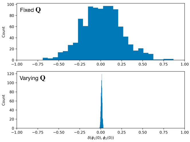
Figure 3: Distribution of $\delta(\phi_{1}(0),\phi_{2}(0))$ over encodings $\phi_{1},\phi_{2}$. Top: $\mathbf{Q}$ is fixed across dimensions for $\phi_{1},\phi_{2}$. Bottom: $\mathbf{Q}$ is varied across dimensions for $\phi_{1},\phi_{2}$.

4.4 Binding as holographic projections

While kernel properties between two encodings with fixed $\mathbf{Q}_{1},\mathbf{Q}_{2}$ can be described simply, the power of GHRR comes from its ability to perform binding while retaining more information regarding its constituents.

Let us first remark that binding two hypervectors in FHRR can be viewed as taking the tensor product of the two hypervectors and then taking the diagonal; i.e. a holographic projection. In the case of GHRR, we can view binding in GHRR as an extension of binding in FHRR. In particular, let the effective dimension of a GHRR encoding be $Dm$ and suppose it is fixed. By modulating $m$, we can interpolate between binding as a parsimonious holographic projection as in the case of FHRR and binding as an equivalent of taking the full tensor product. Figure 4 illustrates the intuition behind binding in FHRR and GHRR as described above.

To illustrate this point, consider two hypervectors $H_{1}=[\mathbf{Q}_{j}\mathbf{\Lambda}_{j}]_{j=1}^{D}$ and $H_{2}=[\mathbf{R}_{j}\mathbf{H}_{j}]_{j=1}^{D}$. Let us focus on the $j$-th matrix-element and let $\mathbf{\Lambda}_{j}=\mathrm{diag}(\lambda_{j1},...,\lambda_{jm})$ and $\mathbf{H}_{j}=\mathrm{diag}(\eta_{j1},...,\eta_{jm})$. Moreover, denote $[\mathbf{Q}_{j}]_{kl}=q_{kl}$ and $[\mathbf{R}_{j}]_{kl}=r_{kl}$. Then the corresponding element of $H_{1}*H_{2}$ is

$$[H_{1}*H_{2}]_{j} =\mathbf{Q}_{j}\mathbf{\Lambda}_{j}\mathbf{R}_{j}\mathbf{H}_{j}=\left[\sum_{n=1}^{m}q_{kn}r_{nl}\lambda_{jn}\eta_{jl}\right]_{k,l=1}^{m}$$ (19)

Thus, each entry of the resulting product of matrix-elements is a linear combination of the entries of the tensor product $\lambda_{j}\eta_{j}^{\top}$, where $\lambda_{j}=[\lambda_{j1},...,\lambda_{jm}]$ and $\eta_{j}=[\eta_{j1},...,\eta_{jm}]$, suggesting that it is some transformed “view” of the tensor product determined by $\mathbf{Q}_{j}$ and $\mathbf{R}_{j}$. Specifically, let $\mathbf{U}_{jl}=\mathbf{Q}_{j}\mathrm{diag}(\mathbf{R}_{j,:,l})$, where $\mathbf{R}_{j,:,l}$ is the $l$-th column of $\mathbf{R}_{j}$. Then Eq. 19 defines a map

$$\varphi_{j}:\lambda_{j}\eta_{j}^{\top}\mapsto\left[\mathbf{U}_{jl}\mathbf{v}_{jl}\right]_{l=1}^{m},$$ (20)

where $\mathbf{v}_{jl}=\lambda_{j}\eta_{jl}$. Clearly, provided $\mathbf{R}_{j}$ has all non-zero entries, $\varphi_{j}$ is invertible.

Let $\lambda=[\lambda_{1},...,\lambda_{D}]$ and $\eta=[\eta_{1},...,\eta_{D}]$ be the concatenations of $\lambda_{1},...,\lambda_{D}$ and $\eta_{1},...,\eta_{D}$, respectively. Now, taking the entire $H_{1}*H_{2}$ into account, we can interpret it as a holographic projection of the tensor product $\lambda\eta^{\top}$, but instead of just taking the diagonal, we take the block-diagonal where blocks are of size $m$ and subsequently transformed by $\mathbf{Q}_{j}$ and $\mathbf{R}_{j}$ as defined by $\varphi_{j}$.

For fixed effective dimension, when $m$ is minimal, i.e. 1, then the block-diagonal is just the diagonal as in FHRR, while, when $m$ is maximal, the block-diagonal is the whole tensor product, i.e. as in Tensor Product Representations [19].

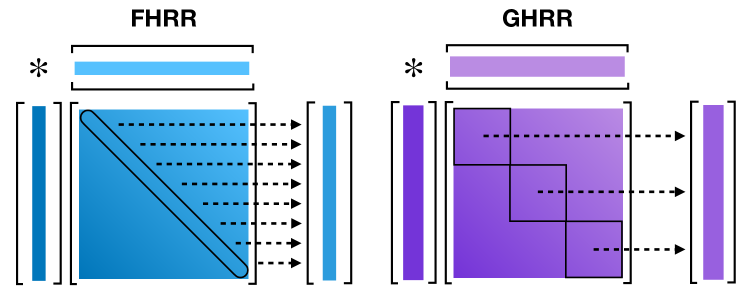
Figure 4: A visualization of binding in FHRR and GHRR. Left: FHRR binding as a projection of the diagonal of the outer product matrix. Right: GHRR binding as a projection of the block-diagonal of the outer product matrix.

From a neural perspective, we can interpret the tensor product between two vectors as representing all possible pairwise connections between the dimensions; i.e. they are fully connected. In contrast, the diagonal projection of a tensor product represents sparse connections where only the corresponding dimensions of the vectors are connected. A block-diagonal projection takes the middle ground, representing connections between nearby dimensions as demarcated by the blocks.

5 Results

5.1 A demonstration of non-commutativity

To demonstrate the non-commutativity of GHRR, we use a simple dictionary as an example. A dictionary associates key-value pairs $\{(k_{i},v_{i})\}_{i=1}^{n}$. The corresponding hypervector that encodes the entire dictionary is

$$\mathbf{H}=\sum_{i=1}^{n}\mathbf{k}_{i}*\mathbf{v}_{i},$$ (21)

where we bold the keys and values to indicate that they are hypervectors. We require that $\mathbf{k}_{i},\mathbf{k}_{j}$ for $i\neq j$ to be quasi-orthogonal. To retrieve $\mathbf{v}_{j}$, we compute

$$\mathbf{k}_{j}^{-1}*\mathbf{H} =\sum_{i=1}^{n}\mathbf{k}_{j}^{-1}\mathbf{k}_{i}*\mathbf{v}_{i}=\mathbf{v}_{j}+\mathrm{noise}.$$ (22)

Figure 5 compares the decoded hypervectors in a nested dictionary for commutative (FHRR) and non-commutative (GHRR) encodings. The dictionary is encoded via $\mathbf{H}=\mathbf{K}_{1}*(\mathbf{K}_{1}*\mathbf{V}_{1}+\mathbf{K}_{2}*\mathbf{V}_{2})+\mathbf{K}_{2}*(\mathbf{K}_{1}*\mathbf{V}_{3}+\mathbf{K}_{2}*\mathbf{V}_{4})$, values are decoded by $\mathbf{V}_{1}^{\prime}=\mathbf{K}_{1}^{-1}*\mathbf{K}_{1}^{-1}*\mathbf{H}$, $\mathbf{V}_{2}^{\prime}=\mathbf{K}_{2}^{-1}*\mathbf{K}_{1}^{-1}*\mathbf{H}$, etc. We observe that the commutative encoding is confused for values with equivalent keys up to permutation, while the non-commutative encoding does not have this issue.

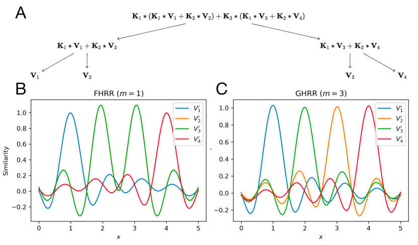
Figure 5: We encode a hypervector $\mathbf{H}=\mathbf{K}_{1}*(\mathbf{K}_{1}*\mathbf{V}_{1}+\mathbf{K}_{2}*\mathbf{V}_{2})+\mathbf{K}_{2}*(\mathbf{K}_{1}*\mathbf{V}_{3}+\mathbf{K}_{2}*\mathbf{V}_{4})$, and retrieve approximate hypervectors $\mathbf{V}_{1}^{\prime}=\mathbf{K}_{1}^{-1}*\mathbf{K}_{1}^{-1}*\mathbf{H}$, $\mathbf{V}_{2}^{\prime}=\mathbf{K}_{2}^{-1}*\mathbf{K}_{1}^{-1}*\mathbf{H}$, etc. We then plot the similarities of the retrieved hypervectors against $\phi(x)$. A decoding is successful if there is a peak at the given value and nowhere else. A. A visualization of the encoded structure. B. We use an FHRR encoding, i.e. a commutative encoding. C. We use a GHRR encoding with $m=3$, i.e. a non-commutative encoding.

5.2 Effect of Q on commutativity

To measure the effect of $\mathbf{Q}$ on the commutativity of GHRR representations, we sample random GHRR hypervectors $H_{1},H_{2}$ and compute the similarity between $H_{1}*H_{2}$ and $H_{2}*H_{1}$. We call the similarity $\delta(H_{1}*H_{2},H_{2}*H_{1})$ the degree of commutativity of the representation. We define the diagonality of a matrix $\mathbf{Q}$ to be $\sum_{j}|\mathbf{Q}_{jj}|/\sum_{j}\sum_{k}|\mathbf{Q}_{jk}|$. Let $\mathbf{Q}_{1},\mathbf{Q}_{2}$ correspond to $H_{1},H_{2}$ respectively.

$$\frac{\sum_{j}|\mathbf{Q}_{jj}|}{\sum_{j}\sum_{k}|\mathbf{Q}_{jk}|}$$

Figure 6 plots the sum of the diagonality of $\mathbf{Q}_{1}$ and $\mathbf{Q}_{2}$ against the degree of commutativity of $H_{1}$ and $H_{2}$. Each point in the figure corresponds to a pair of randomly sampled hypervectors $H_{1},H_{2}$ with corresponding matrices $\mathbf{Q}_{1},\mathbf{Q}_{2}$. Each $\mathbf{Q}_{j}$ is randomly sampled by first sampling a matrix $X\in\mathbb{C}^{m\times m}$, where each component is of the form $a+bi$ with $a,b\sim N(0,1)$. We then define $H(X)=(X+X^{\dagger})/2$ and $\mathbf{Q}_{j}(X)=\exp(iH(X))$. We perform gradient descent on $X$ such that $\mathbf{Q}_{j}(X)$ as diagonality close to the desired value.

We observe that the two quantities are strongly correlated. Moreover, for larger $m$, there is a high probability of sampling a matrix with low diagonality and thus low degree of commutativity.

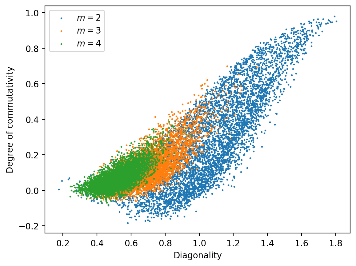
Figure 6: Plot of the sum of the diagonality of $\mathbf{Q}_{1}$ and $\mathbf{Q}_{2}$ against the degree of commutativity of $H_{1}$ and $H_{2}$.

5.3 Decoding accuracy for nested structures

To investigate the effect of $m$, we use a similar setup to the one Section 5.1 but vary the depth of the encoded dictionary. A value is decoded successfully if it has the highest similarity to the decoded hypervector compared to all other values. We plot the decoding accuracy over different depths and values of $m$ in Figure 7A, using a total dimension $Dm^{2}$ of 600. We observe that the larger $m$ is, the longer the high decoding accuracy is sustained for increasing tree depths. However, the overall decoding accuracy also drops faster for larger $m$ after a given tree depth.

In Figure 7B, we use the same procedure as in Figure 7A, but apply the permutation operation to each subtree encoding. Interestingly, we observe that the decoding accuracy is sustained at 100% for longer as we increase the depth of the tree, but decreases sharply after a certain threshold. This is in contrast to Figure 7A, where the decoding accuracy drops below 100% earlier, but decays much more gracefully for larger $m$. The results suggest that using GHRR to encode data structures can provide a simpler implementation (e.g. without permutation) whose decoding accuracy degrades gracefully as the size of the data structure saturates the representation.

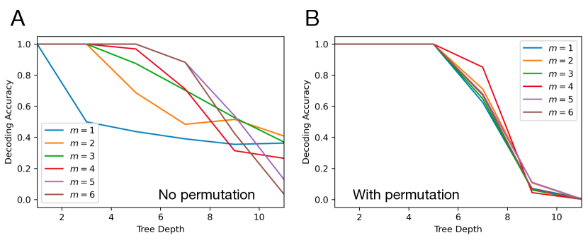
Figure 7: Plot of decoding accuracy for trees of different depths. A. We encode a dictionary as in Figure 5 but with varying depth and GHRR parameter $m$. We use a total dimension of 600 and plot the resulting decoding accuracy. B. Same encoding as in (A) but with permutation applied to each subtree encoding.

We hypothesize that this is due to the exclusivity of the permutation operation; i.e. permutation maps a hypervector to a quasi-orthogonal hypervector, making the decoding quality better. However, this also leads to faster saturation of the tree encoding, leading to a sharp drop in decoding accuracy. On the other hand, the GHRR encoding by itself has a more adjustable range of exclusivity, which, as we will see, is correlated to diagonality, leading to the hypervector having greater memorization capacity [33] albeit for hypervectors that are quasi-orthogonal to a lesser degree.

In addition, we investigate the effect of diagonality on decoding accuracy. Figure 8 plots the decoding accuracy for different tree depths at different levels of diagonality and different values of $m$. 8A, 8B, 8C, and 8D correspond to diagonalities of $0$, $1/3$, $2/3$, and $1$, respectively. We observe that modulating diagonalities from $0$ to $1$ enables us to interpolate between decoding performance similar to that of an FHRR encoding and an FHRR encoding with permutation. Indeed, with a diagonality of $1$, our GHRR encoding becomes commutative, making it functionally equivalent to an FHRR encoding. On the other hand, one can think of a permutation matrix as having diagonality zero (i.e. maximally non-commutative); thus we may expect similar degrees of commutativity for other matrices of diagonality zero. This result suggests that one way to interpret $\mathbf{Q}$ is as a flexible version of the permutation operation that modulates the level of commutativity of the representation.

This observation also provides an explanation for the trends seen in Figure 7A where larger $m$ leads to a decoding accuracy more similar to that of the permutation encoding. For larger $m$, as suggested by Figure 6, we are more likely to sample a matrix with low diagonality, which in turn makes the encoding more non-commutative just like permutation encoding.

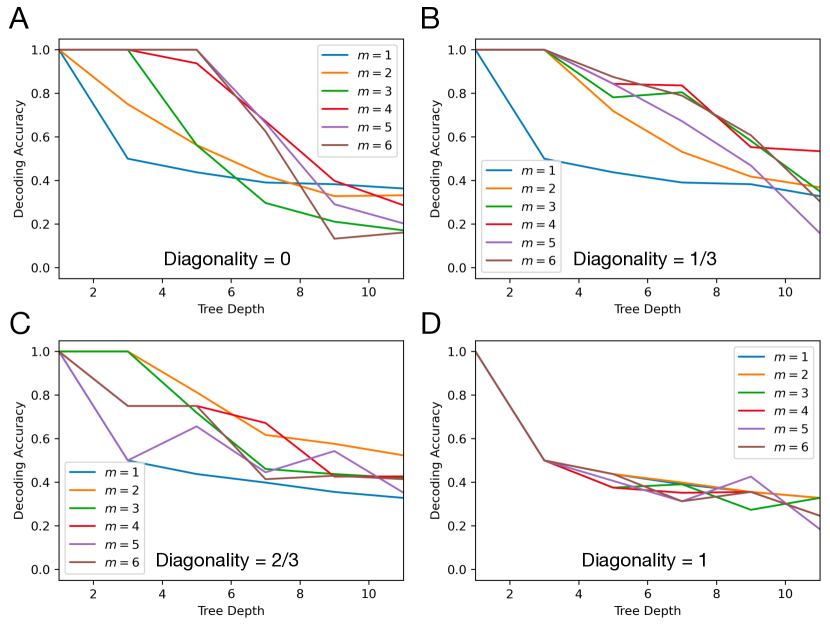
Figure 8: Plot of decoding accuracy for trees of different depths. We encode a dictionary as in Figure 5 but with varying depth and GHRR parameter $m$. We use a total dimension $Dm^{2}$ of 600 and plot the resulting decoding accuracy. A. GHRR encoding with diagonality $0$. B. GHRR encoding with diagonality $1/3$. C. GHRR encoding with diagonality $2/3$. D. GHRR encoding with diagonality $1$.

5.4 Capacity of GHRR representations

Capacity refers to the number of hypervectors one can bundle while still being able to memorize it accurately [33, 31, 34]. We measure capacity by starting with a set $S$ of hypervectors, evenly partitioning it into two sets $X,X^{\prime}$, and forming bundled hypervectors $C_{1}=\sum_{x\in X}x$ and $C_{2}=\sum_{x\in X^{\prime}}x$. We say $X$ is memorized if $\delta(x,C_{1})>\delta(x,C_{2})$ for all $x\in X$. The capacity is the largest $|X|=:N$ for which this property holds. In our case, $S$ consists of bound hypervectors whose components are taken from a finite set $U$. Figure 9 visualizes the intuition behind capacity.

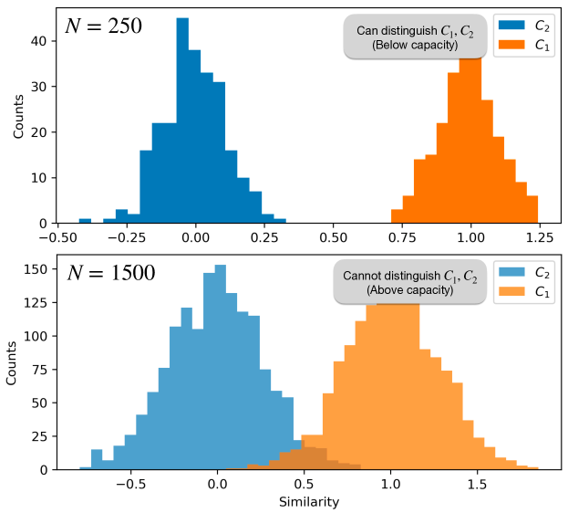
Figure 9: Histogram of similarities between $x$ and $C_{1}$ and $C_{2}$ for all $x\in X$. Above: $C_{1}$ and $C_{2}$ are a bundles of 250 hypervectors. $\delta(x,C_{1})>\delta(x,C_{2})$ for all $x\in X$, so the histograms do not overlap. Below: $C_{1}$ and $C_{2}$ are a bundles of 1500 hypervectors. There exists $x\in C_{1}$ such that $\delta(x,C_{1})\leq\delta(x,C_{2})$, so the histograms overlap.

Specifically, let $n$ be the number of components in the bound hypervector (e.g. $H_{1}*H_{2}*H_{3}$ has 3 components). $U$ consists of $\sqrt[n]{15000}$ randomly generated quasi-orthogonal base hypervectors. $S$ sampled uniformly randomly without replacement from all possible strings of length $n$ with alphabet $U$.

Figure 10 consists of plots of how capacity changes as total dimension $Dm^{2}$ increases for different parameters $m$ and the number of bound components. In Figure 10A, permutations of bound hypervectors are considered distinct, while in Figure 10B, permutations are considered the same and are thus removed.

In Figure 10A, for memorizing the usual base hypervectors (i.e. one bound component hypervectors), there is virtually no difference in capacity between different $m$. Capacity increases approximately linearly with respect to the total dimension $Dm^{2}$. For a larger number of bound components, there is a greater distinction between the capacity for different values of $m$. In particular, $m=1$ (FHRR) is significantly worse. Interestingly, we find that for fixed $m>1$, the difference in capacity for different numbers of bound components is not large. Meanwhile, in Figure 10B, there is a negligible difference between the capacity for different parameters $m$; for all $m$, the capacity scales linearly with respect to the total dimension. Taken together, this suggests that the reason FHRR ($m=1$) performs significantly worse in 10A is due to its inability to distinguish permutations of bound hypervectors. Conversely, increasing $m$ makes the GHRR representation non-commutative and thus able to distinguish between the permutations. At the same time, there is a negligible loss in capacity when we increase $m$ while keeping the total dimension $Dm^{2}$ fixed. These results suggest that GHRR provides a flexible non-commutative representation with no loss in capacity compared to FHRR.

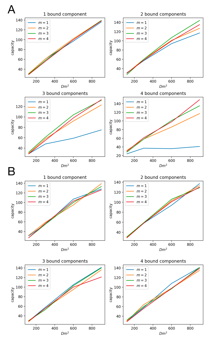
Figure 10: The capacity of bound GHRR representations with varying total dimension $Dm^{2}$ and the number of bound components. A. Plots where permutations are considered distinct; i.e. $A*B\neq B*A$ B. Plots where permutations are considered the same (i.e. $A*B=B*A$) and are thus removed.

6 Discussion

In Section 4.3, we outlined several variations of GHRR with increasing complexity, controlled by whether (1) $\mathbf{Q}$ varies over the dimensions of the GHRR hypervector; and (2) whether $\mathbf{Q}$ depends on the input $\mathbf{x}$. We subsequently explored the simplest variation where $\mathbf{Q}$ is constant and briefly discussed the kernel properties for an encoding with varying $Q$ over the dimensions. In this section, we discuss the other variations and their possibilities for future development.

6.1 Varying Q over dimensions

Varying $Q$ over the dimensions will not substantially affect the shape of the kernel. As we sample $\mathbf{Q}$ and $\mathbf{\Lambda}$ independently of each other, expectations can be factored as in Eq. 10, which suggests that it is enough to know the expected value of $\mathbf{Q}$ to know the shape of the kernel. However, as noted previously, in an encoding scheme that is purely randomly sampled, having varying $\mathbf{Q}$ provides stable behavior as when $D$ increases, the behavior converges to the mean. In addition, having varying $\mathbf{Q}$ over dimensions, as suggested by Eq. 19, places different emphases on the conjunction of hypervectors when binding them together. It is not clear how this affects the characteristics of binding, but it would be an interesting line of investigation.

6.2 Input-dependent Q

As highlighted in Eq. 18, $\mathbf{Q}$ can be thought of as a re-weighting of the kernels corresponding to the elements of the diagonal in $\mathbf{\Lambda}$. Thus, by having $\mathbf{Q}$ depend on the input, we can modulate how important each of the kernels is depending on the context for different pairs of inputs. For example, suppose the kernels $K_{k}$ in the sum correspond to Gaussian kernels with different length scales. Then, for inputs $\mathbf{x},\mathbf{y}\in X$, it is possible to learn a map $Q:X\to\mathcal{H}$ that places emphasis on different kernels depending on the diagonal of the matrix $Q(\mathbf{x})Q(\mathbf{y})^{\dagger}$, which enables us to compare items at different scales depending on context.

Taken together, the above two parameters enable increased complexity and flexibility of GHRR, affecting both the characteristics of binding and the shape and adaptivity of the kernel. It remains to be seen, however, what particular implementations of the map $Q:X\to\mathcal{H}$ would work best for various purposes.

7 Conclusion

In this work, we introduced the GHRR framework, an extension of FHRR, and provided a particular implementation of the framework. We proved that GHRR maintains the theoretical properties of traditional HDC representations and provide empirical demonstrations of quasi-orthogonality. We explored the kernel and binding properties of GHRR and provided an interpretation of binding in GHRR as an interpolation between binding in FHRR and in Tensor Product Representations. We performed empirical experiments on GHRR, demonstrating its flexible non-commutativity, increased decoding accuracy for compositional structures, and improved memorization capacity for bound hypervectors compared to FHRR.

8 Author’s Contributions

Calvin Yeung and Zhuowen Zou wrote the main manuscript text. Calvin Yeung wrote the code to generate the results and prepared all figures. Mohsen Imani provided guidance and feedback. All authors reviewed the manuscript.

9 Funding

This work was supported in part by DARPA Young Faculty Award, National Science Foundation #2127780, #2319198, #2321840 and #2312517, Semiconductor Research Corporation (SRC), Office of Naval Research Young Investigator Program Award, grants #N00014-21-1-2225 and #N00014-22-1-2067, the Air Force Office of Scientific Research under award #FA9550-22-1-0253, and generous gifts from Xilinx and Cisco.

10 Conflict of Interest Statement

Not applicable.

11 Data Availability Statement

Not applicable.

References

- \bibcommenthead
- Krizhevsky et al. [2012] Krizhevsky A, Sutskever I, Hinton GE. ImageNet Classification with Deep Convolutional Neural Networks. In: Advances in Neural Information Processing Systems. vol. 25. Curran Associates, Inc.; 2012. .
- Goodfellow et al. [2014] Goodfellow I, Pouget-Abadie J, Mirza M, Xu B, Warde-Farley D, Ozair S, et al. Generative Adversarial Nets. In: Advances in Neural Information Processing Systems. vol. 27. Curran Associates, Inc.; 2014. .
- Ho et al. [2020] Ho J, Jain A, Abbeel P. Denoising Diffusion Probabilistic Models. In: Advances in Neural Information Processing Systems. vol. 33. Curran Associates, Inc.; 2020. p. 6840–6851.
- Vaswani et al. [2017] Vaswani A, Shazeer N, Parmar N, Uszkoreit J, Jones L, Gomez AN, et al. Attention Is All You Need. In: Advances in Neural Information Processing Systems. vol. 30. Curran Associates, Inc.; 2017. .
- Brown et al. [2020] Brown T, Mann B, Ryder N, Subbiah M, Kaplan JD, Dhariwal P, et al. Language Models Are Few-Shot Learners. In: Advances in Neural Information Processing Systems. vol. 33. Curran Associates, Inc.; 2020. p. 1877–1901.
- Bommasani et al. [2021] Bommasani R, Hudson DA, Adeli E, Altman R, Arora S, von Arx S, et al. On the Opportunities and Risks of Foundation Models. ArXiv. 2021;.
- Kaplan et al. [2020] Kaplan J, McCandlish S, Henighan T, Brown TB, Chess B, Child R, et al.: Scaling Laws for Neural Language Models. arXiv.
- Kanerva [2009] Kanerva P. Hyperdimensional Computing: An Introduction to Computing in Distributed Representation with High-Dimensional Random Vectors. Cognitive Computation. 2009 Jun;1(2):139–159. 10.1007/s12559-009-9009-8.
- Kleyko et al. [2023] Kleyko D, Rachkovskij DA, Osipov E, Rahimi A. A Survey on Hyperdimensional Computing Aka Vector Symbolic Architectures, Part I: Models and Data Transformations. ACM Computing Surveys. 2023 Jul;55(6):1–40. 10.1145/3538531. arxiv:2111.06077. [cs].
- Kleyko et al. [2020] Kleyko D, Rahimi A, Gayler RW, Osipov E. Autoscaling Bloom Filter: Controlling Trade-off between True and False Positives. Neural Computing and Applications. 2020 Apr;32(8):3675–3684. 10.1007/s00521-019-04397-1.
- Frady et al. [2020] Frady EP, Kent SJ, Olshausen BA, Sommer FT. Resonator Networks, 1: An Efficient Solution for Factoring High-Dimensional, Distributed Representations of Data Structures. Neural Computation. 2020 Dec;32(12):2311–2331. 10.1162/neco_a_01331.
- Kleyko et al. [2022] Kleyko D, Davies M, Frady EP, Kanerva P, Kent SJ, Olshausen BA, et al. Vector Symbolic Architectures as a Computing Framework for Emerging Hardware. Proceedings of the IEEE. 2022 Oct;110(10):1538–1571. 10.1109/JPROC.2022.3209104. arxiv:2106.05268. [cs].
- Poduval et al. [2022] Poduval P, Alimohamadi H, Zakeri A, Imani F, Najafi MH, Givargis T, et al. GrapHD: Graph-Based Hyperdimensional Memorization for Brain-Like Cognitive Learning. Frontiers in Neuroscience. 2022;16.
- Hersche et al. [2023] Hersche M, Zeqiri M, Benini L, Sebastian A, Rahimi A. A Neuro-Vector-Symbolic Architecture for Solving Raven’s Progressive Matrices. Nature Machine Intelligence. 2023 Mar;5(4):363–375. 10.1038/s42256-023-00630-8.
- Hersche et al. [2023] Hersche M, Stefano FD, Hofmann T, Sebastian A, Rahimi A. Probabilistic Abduction for Visual Abstract Reasoning via Learning Rules in Vector-symbolic Architectures. In: Annual Conference on Neural Information Processing Systems; 2023. .
- Plate [1995] Plate TA. Holographic Reduced Representations. IEEE Transactions on Neural Networks. 1995 May;6(3):623–641. 10.1109/72.377968.
- Plate [1991] Plate TA. Holographic Reduced Representations: Convolution Algebra for Compositional Distributed Representations. In: International Joint Conference on Artificial Intelligence; 1991. Available from: https://api.semanticscholar.org/CorpusID:1197280.
- Rahimi and Recht [2007] Rahimi A, Recht B. Random Features for Large-Scale Kernel Machines. In: Platt J, Koller D, Singer Y, Roweis S, editors. Advances in Neural Information Processing Systems. vol. 20. Curran Associates, Inc.; 2007. .
- Smolensky [1990] Smolensky P. Tensor Product Variable Binding and the Representation of Symbolic Structures in Connectionist Systems. Artificial Intelligence. 1990 Nov;46(1):159–216. 10.1016/0004-3702(90)90007-M.
- Kleyko et al. [2023] Kleyko D, Rachkovskij D, Osipov E, Rahimi A. A survey on hyperdimensional computing aka vector symbolic architectures, part ii: Applications, cognitive models, and challenges. ACM Computing Surveys. 2023;55(9):1–52.
- Gayler [1998] Gayler RW.: Multiplicative Binding, Representation Operators & Analogy (Workshop Poster). Available from: http://cogprints.org/502/.
- Plate [1994] Plate TA. Distributed representations and nested compositional structure. Citeseer; 1994.
- Frady et al. [2022] Frady EP, Kleyko D, Kymn CJ, Olshausen BA, Sommer FT. Computing on Functions Using Randomized Vector Representations (in Brief). In: Neuro-Inspired Computational Elements Conference. Virtual Event USA: ACM; 2022. p. 115–122.
- Poduval et al. [2022] Poduval P, Zakeri A, Imani F, Alimohamadi H, Imani M. Graphd: Graph-based hyperdimensional memorization for brain-like cognitive learning. Frontiers in Neuroscience. 2022;p. 5.
- Nunes et al. [2022] Nunes I, Heddes M, Givargis T, Nicolau A, Veidenbaum A. GraphHD: Efficient graph classification using hyperdimensional computing. In: 2022 Design, Automation & Test in Europe Conference & Exhibition (DATE). IEEE; 2022. p. 1485–1490.
- Gayler and Levy [2009] Gayler RW, Levy SD. A distributed basis for analogical mapping. In: New Frontiers in Analogy Research; Proc. of 2nd Intern. Analogy Conf. vol. 9; 2009. .
- Osipov et al. [2022] Osipov E, Kahawala S, Haputhanthri D, Kempitiya T, De Silva D, Alahakoon D, et al. Hyperseed: Unsupervised learning with vector symbolic architectures. IEEE Transactions on Neural Networks and Learning Systems. 2022;.
- Kim et al. [2018] Kim Y, Imani M, Rosing TS. Efficient human activity recognition using hyperdimensional computing. In: Proceedings of the 8th International Conference on the Internet of Things; 2018. p. 1–6.
- Imani et al. [2018] Imani M, Huang C, Kong D, Rosing T. Hierarchical hyperdimensional computing for energy efficient classification. In: Proceedings of the 55th Annual Design Automation Conference; 2018. p. 1–6.
- Imani et al. [2019] Imani M, Bosch S, Datta S, Ramakrishna S, Salamat S, Rabaey JM, et al. Quanthd: A quantization framework for hyperdimensional computing. IEEE Transactions on Computer-Aided Design of Integrated Circuits and Systems. 2019;39(10):2268–2278.
- Thomas et al. [2022] Thomas A, Dasgupta S, Rosing T. A Theoretical Perspective on Hyperdimensional Computing. Journal of Artificial Intelligence Research. 2022 Jan;72:215–249. 10.1613/jair.1.12664.
- Gayler [2004] Gayler RW. Vector symbolic architectures answer Jackendoff’s challenges for cognitive neuroscience. arXiv preprint cs/0412059. 2004;.
- Frady et al. [2018] Frady EP, Kleyko D, Sommer FT. A Theory of Sequence Indexing and Working Memory in Recurrent Neural Networks. Neural Computation. 2018 Jun;30(6):1449–1513. 10.1162/neco_a_01084.
- Rahimi et al. [2017] Rahimi A, Datta S, Kleyko D, Frady EP, Olshausen B, Kanerva P, et al. High-dimensional computing as a nanoscalable paradigm. IEEE Transactions on Circuits and Systems I: Regular Papers. 2017;64(9):2508–2521.