From Local to Global Order: A Theory of Neural Synaptic Balance

Abstract.

We develop a general theory of neural synaptic balance and how it can emerge or be enforced in neural networks. For a given additive cost function $R$ (regularizer), a neuron is said to be in balance if the total cost of its input weights is equal to the total cost of its output weights. The basic example is provided by feedforward networks of ReLU units trained with $L_{2}$ regularizers, which exhibit balance after proper training. The theory explains this phenomenon and extends it in several directions. The first direction is the extension to bilinear and other activation functions. The second direction is the extension to more general regularizers, including all $L_{p}$ ($p>0$) regularizers. The third direction is the extension to non-layered architectures, recurrent architectures, convolutional architectures, as well as architectures with mixed activation functions. Gradient descent on the error function alone does not converge in general to a balanced state where every neuron is in balance, even when starting from a balanced state. However, gradient descent on the regularized error function must converge to a balanced state, and thus network balance can be used to assess learning progress. The theory is based on two local neuronal operations: scaling which is commutative, and balancing which is not commutative. Finally, and most importantly, given any initial set of weights, when local balancing operations are applied to each neuron in a stochastic manner, global order always emerges through the convergence of the stochastic balancing algorithm to the same unique set of balanced weights. The reason for this convergence is the existence of an underlying strictly convex optimization problem where the relevant variables are constrained to a linear, only architecture-dependent, manifold. The theory is corroborated through various simulations carried out on benchmark data sets. Scaling and balancing operations are entirely local and thus physically plausible in biological and neuromorphic networks.

Keywords: neural networks; deep learning; activation functions; regularization; scaling; neural balance.

1. Introduction

One of the most common complaints against neural networks is that they provide at best “black-box” solutions to problems. In particular, when large neural networks are trained on complex tasks, they produce large arrays of synaptic weights that have no clear structure and are difficult to interpret. Thus finding any kind of structure in the weights of large neural networks is of great interest. Here we study a particular kind of structure we call neural synaptic balance and the conditions under which it emerges. Neural synaptic balance is different from the biological notion of balance between excitation and inhibition [12, 10, 13, 17, 23]. We use the term to refer to any systematic relationship between the input and output synaptic weights of individual neurons or layers of neurons. Here we consider the case where the cost of the input weights is equal to the cost of the output weights, where the cost is defined by some regularizer. One of the most basic examples of such a relationship is when the sum of the squares of the input weights of a neuron is equal to the sum of the squares of its output weights.

Basic Example: The basic example where this happens is with a neuron with a ReLU activation function inside a network trained to minimize an error function with $L_{2}$ regularization. If we multiply the incoming weights of the neuron by some $\lambda>0$ and divide the outgoing weights of the neuron by the same $\lambda$, it is easy to see that this double scaling operation does not affect in any way the contribution of the neuron to the rest of the network. Thus, any component of the error function that depends only on the input-output function of the network is unchanged. However, the value of the $L_{2}$ regularizer changes with $\lambda$ and we can ask what is the value of $\lambda$ that minimizes the corresponding contribution given by:

$$\sum_{i\in IN}(\lambda w_{i})^{2}+\sum_{i\in OUT}(w_{i}/\lambda)^{2}=\lambda^{2}A+\frac{1}{\lambda^{2}}B$$ (1.1)

where $IN$ and $OUT$ denote the set of incoming and outgoing weights respectively, $A=\sum_{i\in IN}w_{i}^{2}$, and $B=\sum_{i\in OUT}w_{i}^{2}$. The product of the two terms on the right-hand side of Equation 1.1 is equal to $AB$ and does not depend on $\lambda$. Thus, the minimum is achieved when these two terms are equal, which yields: $(\lambda^{*})^{4}=B/A$ for the optimal $\lambda^{*}$. The corresponding new set of weights, $v_{i}=\lambda^{*}w_{i}$ for the input weights and $v_{i}=w_{i}/\lambda^{*}$ for the outgoing weights, must be balanced: $\sum_{i\in IN}v_{i}^{2}=\sum_{i\in OUT}v_{i}^{2}$. This is because the optimal scaling factor for these rescaled weights must be $\lambda^{*}=1$. Furthermore, if an entire network of ReLU neurons is properly trained using a standard error function with an $L_{2}$ regularizer, at the end of training one observes a remarkable phenomenon: for each ReLU neuron, the norm of the incoming synaptic weights is approximately equal to the norm of the outgoing synaptic weights, i.e. every neuron is balanced.

There have been isolated previous studies of this kind of synaptic balance [9, 25] under special conditions. For instance, in [9], it is shown that if a deep network is initialized in a balanced state with respect to the sum of squares metric, and if training progresses with an infinitesimal learning rate, then balance is preserved throughout training. Here, we take a different approach aimed at uncovering the generality of neuronal balance phenomena, the learning conditions under which they occur, as well as new local balancing algorithms and their convergence properties. We explain and study neural synaptic balance in its generality in terms of activation functions, regularizers, network architectures, and training stages. In particular, we systematically answer questions such as: Why does balance occur? Does it occur only with ReLU neurons? Does it occur only with $L_{2}$ regularizers? Does it occur only in fully connected feedforward architectures (as opposed to, for instance, locally connected, convolutional, or recurrent architectures)? Does it occur only at the end of training? In the process of answering these questions, we introduce local scaling and balancing operations for individual neurons or entire neural layers. Furthermore, we show that when these local operations are applied stochastically, a global balanced state always emerges, and this state is unique and depends only on the initial weights, but not on the order in which the neurons are balanced.

2. Homogeneous and BiLU Activation Functions

In this section, we generalize the basic example of the introduction from the standpoint of the activation functions. In particular, we consider homogeneous activation functions (defined below). The importance of homogeneity has been previously identified in somewhat different contexts [19]. Intuitively, homogeneity is a form of linearity with respect to weight scaling and thus it is useful to motivate the concept of homogeneous activation functions by looking at other notions of linearity for activation functions. This will also be useful for Section 6 where even more general classes of activation functions are considered.

2.1. Additive Activation Functions

Definition 2.1.

A neuronal activation function $f:\mathbb{R}\to\mathbb{R}$ is additively linear if and only if $f(x+y)=f(x)=(f(y)$ for any real numbers $x$ and $y$.

Proposition 2.2.

The class of additively linear activation functions is exactly equal to the class of linear activation functions, i.e., activation functions of the form $f(x)=ax$.

Proof.

Obviously linear activation functions are additively linear. Conversely, if $f$ is additively linear, the following three properties are true:

(1) One must have: $f(nx)=nf(x)$ and $f(x/n)=f(x)/n$ for any $x\in\mathbb{R}$ and any $n\in\mathbb{N}$. As a result, $f(n/m)=nf(1)/m$ for any integers $n$ and $m$ ($m\not=0$).

(2) Furthermore, $f(0+0)=f(0)+f(0)$ which implies: $f(0)=0$.

(3) And thus $f(x-x)=f(x)+f(-x)=0$, which in turn implies that $f(-x)=-f(x)$.

From these properties, it is easy to see that $f$ must be continuous, with $f(x)=xf(1)$, and thus $f$ must be linear. ∎

2.2. Multiplicative Activation Functions

Definition 2.3.

A neuronal activation function $f:\mathbb{R}\to\mathbb{R}$ is multiplicative if and only if $f(xy)=f(x)(f(y)$ for any real numbers $x$ and $y$.

Proposition 2.4.

The class of continuous multiplicative activation functions is exactly equal to the class of functions comprising the functions: $f(x)=0$ for every $x$, $f(x)=1$ for every $x$, and all the even and odd functions satisfying $f(x)=x^{c}$ for $x\geq 0$, where $c$ is any constant in $\mathbb{R}$.

Proof.

It is easy to check the functions described in the proposition are multiplicative. Conversely, assume $f$ is multiplicative. For both $x=0$ and $x=1$, we must have $f(x)=f(xx)=f(x)f(x)$ and thus $f(0)$ is either 0 or 1, and similarly for $f(1)$. If $f(1)=0$, then for any $x$ we must have $f(x)=0$ because: $f(x)=f(1x)=f(1)f(x)=0$. Likewise, if $f(0)=1$, then for any $x$ we must have $f(x)=1$ because: $1=f(0)=f(0x)=f(0)f(x)=f(x)$. Thus, in the rest of the proof, we can assume that $f(0)=0$ and $f(1)=1$. By induction, it is easy to see that for any $x\geq 0$ we must have: $f(x^{n})=f(x)^{n}$ and $f(x^{1/n})=(f(x))^{1/n}$ for any integer (positive or negative). As a result, for any $x\in\mathbb{R}$ and any integers $n$ and $m$ we must have: $f(x^{n/m})=f(x)^{n/m}$. By continuity this implies that for any $x\geq 0$ and any $r\in R$, we must have: $f(x^{r})=f(x)^{r}$. Now there is some constant $c$ such that: $f(e)=e^{c}$. And thus, for any $x>0$, $f(x)=f(e^{\log x})=[f(e)]^{\log x}=e^{c\log x}=x^{c}$. To address negative values of $x$, note that we must have $f[(-1)(-1=f(1)=1f(-1)^{2}$. Thus, $f(-1)$ is either equal to 1 or to -1. Since for any $x>0$ we have $f(-x)=f(-1)f(x)$, we see that if $f(-1)=1$ the function must be even ($f(-x)=f(x)=x^{c}$), and if $f(-1)=-1$ the function must be odd ($f(-x)=-f(x)$). ∎

We will return to multiplicative activation function in a later section.

2.3. Linearly Scalable Activation Functions

Definition 2.5.

A neuronal activation function $f:\mathbb{R}\to\mathbb{R}$ is linearly scalable if and only if $f(\lambda x)=\lambda f(x)$ for every $\lambda\in\mathbb{R}$.

Proposition 2.6.

The class of linearly scalable activation functions is exactly equal to the class of linear activation functions, i.e., activation functions of the form $f(x)=ax$.

Proof.

Obviously, linear activation functions are linearly scalable. For the converse, if $f$ is linearly multiplicative we must have $f(\lambda x)=\lambda f(x)=xf(\lambda)$ for any $x$ and any $\lambda$. By taking $\lambda=1$, we get $f(x)=f(1)x$ and thus $f$ is linear. ∎

Thus the concepts of linearly additive or linearly scalable activation function are of limited interest since both of them are equivalent to the concept of linear activation function. A more interesting class is obtained if we consider linearly scalable activation functions, where the scaling factor $\lambda$ is constrained to be positive ($\lambda>0$), also called homogeneous functions.

2.4. Homogeneous Activation Functions

Definition 2.7.

(Homogeneous) A neuronal activation function $f:\mathbb{R}\to\mathbb{R}$ is homogeneous if and only if: $f(\lambda x)=\lambda f(x)$ for every $\lambda\in\mathbb{R}$ with $\lambda>0$.

Remark 2.8.

Note that if $f$ is homogeneous, $f(\lambda 0)=\lambda f(0)=f(0)$ for any $\lambda>0$ and thus $f(0)=0$. Thus it makes no difference in the definition of homogeneous if we set $\lambda\geq 0$ instead of $\lambda>0)$.

Remark 2.9.

Clearly, linear activation functions are homogeneous. However, there exists also homogeneous functions that are non-linear, such as ReLU or leaky ReLU activation functions.

We now provide a full characterization of the class of homogeneous activation functions.

2.5. BiLU Activation Functions

We first define a new class of activation functions, corresponding to bilinear units (BiLU), consisting of two half-lines meeting at the origin. This class contains all the linear functions, as well as the ReLU and leaky ReLU functions, and many other functions.

Definition 2.10.

(BiLU) A neuronal activation function $f:\mathbb{R}\to\mathbb{R}$ is bilinear (BiLU) if and only if $f(x)=ax$ when $x<0$, and $f(x)=bx$ when $x\geq 0$, for some fixed parameters $a$ and $b$ in $\mathbb{R}$.

These include linear units ($a=b$), ReLU units ($a=0,b=1$), leaky ReLU ($a=\epsilon;b=1$) units, and symmetric linear units ($a=-b$), all of which can also be viewed as special cases of piece-wise linear units [27], with a single hinge. One advantage of ReLU and more generally BiLU neurons, which is very important during backpropagation learning, is that their derivative is very simple and can only take one of two values ($a$ or $b$).

Proposition 2.11.

A neuronal activation function $f:\mathbb{R}\to\mathbb{R}$ is homogeneous if and only if it is a BiLU activation function.

Proof.

Every function in BiLU is clearly homogeneous. Conversely, any homogeneous function $f$ must satisfy: (1) $f(0x)=0f(x)=f(0)=0$; (2)$f(x)=f(1x)=f(1)x$ for any positive $x$; and (3) $f(x)=f(-u)=f(-1)u=-f(-1)x$ for any negative $x$. Thus $f$ is in BiLU with $a=-f(-1)$ and $b=f(1)$. ∎

In Appendix A, we provide a simple proof that networks of BiLU neurons, even with a single hidden layer, have universal approximation properties. In the next two sections, we introduce two fundamental neuronal operations, scaling and balancing, that can be applied to the incoming and outgoing synaptic weights of neurons with BiLU activation functions.

3. Scaling

Definition 3.1.

(Scaling) For any BiLU neuron $i$ in network and any $\lambda>0$, we let $S_{\lambda}(i)$ denote the synaptic scaling operation by which the incoming connection weights of neuron $i$ are multiplied by $\lambda$ and the outgoing connection weights of neuron $i$ are divided by $\lambda$.

Note that because of the homogeneous property the scaling operation does not change how neuron $i$ affects the rest of the network. In particular, the input-output function of the overall network remains unchanged after scaling neuron $i$ bt any $\lambda>0$. Note also that scaling always preserves the sign of the synaptic weights to which it is applied, and the scaling operation can never convert a non-zero synaptic weight into a zero synaptic weight, or vice versa.

As usual, the bias is treated here as an additional synaptic weight emanating from a unit clamped to the value one. Thus scaling is applied to the bias.

Proposition 3.2.

(Commutativity of Scaling) Scaling operations applied to any pair of BiLU neurons $i$ and $j$ in a neural network commute: $S_{\lambda}(i)S_{\mu}(j)=S_{\mu}(j)S_{\lambda}(i)$, in the sense that the resulting network weights are the same, regardless of the order in which the scaling operations are applied. Furthermore, for any BiLU neuron $i$: $S_{\lambda}(i)S_{\mu}(i)=S_{\mu}(i)S_{\lambda}(i)=S_{\lambda\mu}(i)$.

This is obvious. As a result, any set $I$ of BiLU neurons in a network can be scaled simultaneously or in any sequential order while leading to the same final configuration of synaptic weights. If we denote by $1,2,\dots,n$ the neurons in $I$, we can for instance write: $\prod_{i\in I}S_{\lambda_{i}}(i)=\prod_{\sigma(i)\in I}S_{\lambda_{\sigma(i)}}(\sigma(i))$ for any permutation $\sigma$ of the neurons. Likewise, we can collapse operations applied to the same neuron. For instance, we can write: $S_{5}(1)S_{2}(2)S_{3}(1)S_{4}(2)=S_{15}(1)S_{8}(2)=S_{8}(2)S_{15}(1)$

Definition 3.3.

(Coordinated Scaling) For any set $I$ of BiLU neurons in a network and any $\lambda>0$, we let $S_{\lambda}(I)$ denote the synaptic scaling operation by which all the neurons in $I$ are scaled by the same $\lambda$.

4. Balancing

Definition 4.1.

(Balancing) Given a BiLU neuron in a network, the balancing operation $B(i)$ is a particular scaling operation $B(i)=S_{\lambda^{*}}(i)$, where the scaling factor $\lambda^{*}$ is chosen to optimize a particular cost function, or regularizer, asociated with the incoming and outgoing weights of neuron $i$.

For now, we can imagine that this cost function is the usual $L_{2}$ (least squares) regularizer, but in the next section, we will consider more general classes of regularizers and study the corresponding optimization process. For the $L_{2}$ regularizer, as shown in the next section, this optimization process results in a unique value of $\lambda^{*}$ such that sum of the squares of the incoming weights is equal to the sum of the squares of the outgoing weights, hence the term “balance”. Note that obviously $B(B(i))=B(i)$ and that, as a special case of scaling operation, the balancing operation does not change how neuron $i$ contributes to the rest of the network, and thus it leaves the overall input-output function of the network unchanged.

Unlike scaling operations, balancing operations in general do not commute as balancing operations (they still commute as scaling operations). Thus, in general, $B(i)B(j)\not=B(j)B(i)$. This is because if neuron $i$ is connected to neuron $j$, balancing $i$ will change the connection between $i$ and $j$, and, in turn, this will change the value of the optimal scaling constant for neuron $j$ and vice versa. However, if there are no non-zero connections between neuron $i$ and neuron $j$ then the balancing operations commute since each balancing operation will modify a different, non-overlapping, set of weights.

Definition 4.2.

(Disjoint neurons) Two neurons $i$ and $j$ in a neural network are said to be disjoint if there are no non-zero connections between $i$ and $j$.

Thus in this case $B(i)B(j)=S_{\lambda^{*}}(i)S_{\mu^{*}}(j)=S_{\mu^{*}}(j)S_{\lambda^{*}}(i)=B(j)B(i)$. This can be extended to disjoint sets of neurons.

Definition 4.3.

(Disjoint Set of Neurons) A set $I$ of neurons is said to be disjoint if for any pair $i$ and $j$ of neurons in $I$ there are no non-zero connections between $i$ and $j$.

For example, in a layered feedforward network, all the neurons in a layer form a disjoint set, as long as there are no intra-layer connections or, more precisely, no non-zero intra-layer connections. All the neurons in a disjoint set can be balanced in any order resulting in the same final set of synaptic weights. Thus we have:

Proposition 4.4.

If we index by $1,2,\dots,n$ the neurons in a disjoint set $I$ of BiLU neurons in a network, we have: $\prod_{i\in I}B(i)=\prod_{i\in I}S_{\lambda^{*}_{i}}(i)=\prod_{\sigma(i)\in I}S_{\lambda^{*}_{\sigma(i)}}(\sigma(i))=\prod_{\sigma(i)\in I}B(\sigma(i))$ for any permutation $\sigma$ of the neurons.

Finally, we can define the coordinated balancing of any set $I$ of BiLU neurons (disjoint or not disjoint).

Definition 4.5.

(Coordinated Balancing) Given any set $I$ of BiLU neurons (disjoint or not disjoint) in a network, the coordinated balacing of these neurons, written as $B_{\lambda^{*}}(I)$, corresponds to coordinated scaling all the neurons in $I$ by the same factor $\lambda^{*}$, Where $\lambda^{*}$ minimizes the cost functions of all the weights, incoming and outgoing, associated with all the neurons in $I$.

Remark 4.6.

While balancing corresponds to a full optimization of the scaling operation, it is also possible to carry a partial optimization of the scaling operation by choosing a scaling factor that reduces the corresponding contribution to the regularizer without minimizing it.

5. General Framework and Single Neuron Balance

In this section, we generalize the kinds of regularizer to which the notion of neuronal synaptic balance can be applied, beyond the usual $L_{2}$ regularizer and derive the corresponding balance equations. Thus we consider a network (feedforward or recurrent) where the hidden units are BiLU units. The visible units can be partitioned into input units and output units. For any hidden unit $i$, if we multiply all its incoming weights $IN(i)$ by some $\lambda>0$ and all its outgoing weights $OUT(i)$ by $1/\lambda$ the overall function computed by the network remains unchanged due to the BiLU homogeneity property. In particular, if there is an error function that depends uniquely on the input-output function being computed, this error remains unchanged by the introduction of the multiplier $\lambda$. However, if there is also a regularizer $R$ for the weights, its value is affected by $\lambda$ and one can ask what is the optimal value of $\lambda$ with respect to the regularizer, and what are the properties of the resulting weights. This approach can be applied to any regularizer. For most practical purposes, we can assume that the regularizer is continuous in the weights (hence in $\lambda$) and lower-bounded. Without any loss of generality, we can assume that it is lower-bounded by zero. If we want the minimum value to be achieved by some $\lambda>0$, we need to add some mild condition that prevents the minimal value to be approached as $\lambda\to 0^{)}$, or as $\lambda\to+\infty$. For instance, it is enough if there is an interval $[a,b]$ with $0<a<b$ where $R$ achieves a minimal value $R_{min}$ and $R\geq R_{min}$ in the intervals $(0,a]$ and $[b,+\infty)$. Additional (mild) conditions must be imposed if one wants the optimal value of $\lambda$ to be unique, or computable in closed form (see Theorems below). Finally, we want to be able to apply the balancing approach

Thus, we consider overall regularized error functions, where the regularizer is very general, as long as it has an additive form with respect to the individual weights:

$${\mathcal{E}}(W)=E(W)+R(W)\quad{\rm with}\quad R(W)=\sum_{w}g_{w}(w)$$ (5.1)

where $W$ denotes all the weights in the network and $E(W)$ is typically the negative log-likelihood (LMS error in regression tasks, or cross-entropy error in classification tasks). We assume that the $g_{w}$ are continuous, and lower-bounded by 0. To ensure the existence and uniqueness of minimum during the balancing of any neuron, We will assume that each function $g_{w}$ depends only on the magnitude $|w|$ of the corresponding weight, and that $g_{w}$ is monotonically increasing from 0 to $+\infty$ ($g_{w}(0)=0$ and $\lim_{x\to+\infty}g_{w}(x)=+\infty$). Clearly, $L_{2},L_{1}$ and more generally all $L_{p}$ regularizers are special cases where, for $p>0$, $L^{p}$ regularization is defined by: $R(W)=\sum_{w}|w|^{p}$.

When indicated, we may require also that the functions $g_{w}$ be continuously differentiable, except perhaps at the origin in order to be able to differentiate the regularizer with respect to the $\lambda$’s and derive closed form conditions for the corresponding optima. This is satisfied by all forms of $L_{p}$ regularization, for $p>0$.

Remark 5.1.

Often one introduces scalar multiplicative hyperparameters to balance the effect of $E$ and $R$, for instance in the form: ${\mathcal{E}}=E+\beta R$. These cases are included in the framework above: multipliers like $\beta$ can easily be absorbed into the functions $g_{w}$ above.

Theorem 5.2.

(General Balance Equation). Consider a neural network with BiLU activation functions in all the hidden units and overall error function of the form:

$${\mathcal{E}}=E(W)+R(W)\quad{\rm with}\quad R(W)=\sum_{w}g_{w}(w)$$ (5.2)

where each function $g_{w}(w)$ is continuous, depends on the magnitude $|w|$ alone, and grows monotonically from $g_{w}(0)=0$ to $g_{w}(+\infty)=+\infty$. For any setting of the weights $W$ and any hidden unit $i$ in the network and any $\lambda>0$ we can multiply the incoming weights of $i$ by $\lambda$ and the outgoing weights of $i$ by $1/\lambda$ without changing the overall error $E$. Furthermore, there exists a unique value $\lambda^{*}$ where the corresponding weights $v$ ($v=\lambda^{*}w$ for incoming weights, $v=w/\lambda^{*}$ for the outgoing weights) achieve the balance equation:

$$\sum_{v\in IN(i)}g_{w}(v)=\sum_{w\in OUT(i)}g_{w}(v)$$ (5.3)

Proof.

Under the assumptions of the theorem, $E$ is unchanged under the rescaling of the incoming and outgoing weights of unit $i$ due to the homogeneity property of BiLUs. Without any loss of generality, let us assume that at the beginning: $\sum_{w\in IN(i)}g_{w}(w)<\sum_{w\in OUT(i)}g_{w}(w)$. As we increase $\lambda$ from 1 to $+\infty$, by the assumptions on the functions $g_{w}$, the term $\sum_{w\in IN(i)}g_{w}(\lambda w)$ increases continuously from its initial value to $+\infty$, whereas the term $\sum_{w\in OUT(i)}g_{w})w/\lambda)$ decreases continuously from its initial value to $0$. Thus, there is a unique value $\lambda^{*}$ where the balance is realized. If at the beginning $\sum_{w\in IN(i)}g_{w}(w)>\sum_{w\in OUT(i)}g_{w}(w)$, then the same argument is applied by decreasing $\lambda$ from 1 to 0. ∎

Remark 5.3.

For simplicity, here and in other sections, we state the results in terms of a network of BiLU units. However, the same principles can be applied to networks where only a subset of neurons are in the BiLU class, simply by applying scaling and balancing operations to only those neurons. Furthermore, not all BiLU neurons need to have the same BiLU activation functios. For instance, the results still hold for a mixed network containing both ReLU and linear units.

Remark 5.4.

In the setting of Theorem 5.2, the balance equations do not necessarily minimize the corresponding regularization term. This is addressed in the next theorem.

Remark 5.5.

Finally, zero weights ($w=0$) can be ignored entirely as they play no role in scaling or balancing. Furthermore, if all the incoming or outgoing weights of a hidden unit were to be zero, it could be removed entirely from the network

Theorem 5.6.

(Balance and Regularizer Minimization) We now consider the same setting as in Theorem 5.2, but in addition we assume that the functions $g_{w}$ are continuously differentiable, except perhaps at the origin. Then, for any neuron, there exists at least one optimal value $\lambda^{*}$ that minimizes $R(W)$. Any optimal value must be a solution of the consistency equation:

$$\lambda^{2}\sum_{w\in IN(i)}wg^{\prime}_{w}(\lambda w)=\sum_{w\in OUT(i)}wg^{\prime}_{w}(w/\lambda)$$ (5.4)

Once the weights are rebalanced accordingly, the new weights must satisfy the generalized balance equation:

$$\sum_{w\in IN(i)}wg^{\prime}(w)=\sum_{w\in OUT(i)}wg^{\prime}(w)$$ (5.5)

In particular, if $g_{w}(w)=|w|^{p}$ for all the incoming and outgoing weights of neuron $i$, then the optimal value $\lambda^{*}$ is unique and equal to:

$$\lambda^{*}=\Bigl{(}\frac{\sum_{w\in OUT(i)}|w|^{p}}{\sum_{w\in IN(i)}|w|^{p}}\Bigr{)}^{1/2p}=\Bigl{(}\frac{||OUT(i)||_{p}}{||IN(i)||_{p}}\Bigr{)}^{1/2}$$ (5.6)

The decrease $\Delta R\geq 0$ in the value of the $L_{p}$ regularizer $R=\sum_{w}|w|^{p}$ is given by:

$$\Delta R=\biggl{(}\bigl{(}\sum_{w\in IN(i)}|w|^{p}\bigr{)}^{1/2}-\bigl{(}\sum_{w\in OUT(i)}|w|^{p}\bigr{)}^{1/2}\biggr{)}^{2}$$ (5.7)

After balancing neuron $i$, its new weights satisfy the generalized $L_{p}$ balance equation:

$$\sum_{w\in IN(i)}|w|^{p}=\sum_{w\in OUT(i)}|w|^{p}$$ (5.8)

Proof.

Due to the additivity of the regularizer, the only component of the regularizer that depends on $\lambda$ has the form:

$$R(\lambda)=\sum_{w\in IN(i)}g_{w}(\lambda w)+\sum_{w\in OUT(i)}g_{w}(w/\lambda)$$ (5.9)

Because of the properties of the functions $g_{w}$, $R_{\lambda}$ is continously differentiable and strictly bounded below by 0. So it must have a minimum, as a function of $\lambda$ where its derivative is zero. Its derivative with respect to $\lambda$ has the form:

$$R^{\prime}(\lambda)=\sum_{w\in IN(i)}wg^{\prime}_{w}(\lambda w)+\sum_{w\in OUT(i)}(-w/\lambda^{2})g^{\prime}_{w}(w/\lambda)$$ (5.10)

Setting the derivative to zero, gives:

$$\lambda^{2}\sum_{w\in IN(i)}wg^{\prime}_{w}(\lambda w)=\sum_{w\in OUT(i)}wg^{\prime}_{w}(w/\lambda)$$ (5.11)

Assuming that the left-hand side is non-zero, which is generally the case, the optimal value for $\lambda$ must satisfy:

$$\lambda=\Bigl{(}\frac{\sum_{w\in OUT(i)}wg^{\prime}_{w}(w/\lambda)}{\sum_{w\in IN(i)}wg^{\prime}_{w}(\lambda w)}\Bigr{)}^{1/2}$$ (5.12)

If the regularizing function is the same for all the incoming and outgoing weights ($g_{w}=g$), then the optimal value $\lambda$ must satisfy:

$$\lambda=\Bigl{(}\frac{\sum_{w\in OUT(i)}wg^{\prime}(w/\lambda)}{\sum_{w\in IN(i)}wg^{\prime}(\lambda w)}\Bigr{)}^{1/2}$$ (5.13)

In particular, if $g(w)=|w|^{p}$ then $g(w)$ is differentiable except possibly at 0 and $g^{\prime}(w)=s(w)p|w|^{p-1}$, where $s(w)$ denotes the sign of the weight $w$. Substituting in Equation 5.13, the optimal rescaling $\lambda$ must satisfy:

$$\lambda^{*}=\Bigl{(}\frac{\sum_{w\in OUT(i)}ws(w)|w|^{p-1}}{\sum_{w\in IN(i)}w|ws(w)|^{p-1}}\Bigr{)}^{1/2p}=\Bigl{(}\frac{\sum_{w\in OUT(i)}|w|^{p}}{\sum_{w\in IN(i)}|w|^{p}}\Bigr{)}^{1/2p}=\Bigl{(}\frac{||OUT(i)||_{p}}{||IN(i)||_{p}}\Bigr{)}^{1/2}$$ (5.14)

At the optimum, no further balancing is possible, and thus $\lambda^{*}=1$. Equation 5.11 yields immediately the generalized balance equation to be satisfied at the optimum:

$$\sum_{w\in IN(i)}wg^{\prime}(w)=\sum_{w\in OUT(i)}wg^{\prime}(w)$$ (5.15)

In the case of $L_{P}$ regularization, it is easy to check by applying Equation 5.15, or by direct calculation that:

$$\sum_{w\in IN(i)}|\lambda^{*}w|^{p}=\sum_{w\in OUT(i)}|w/\lambda^{*}|^{p}$$ (5.16)

which is the generalized balance equation. Thus after balancing neuron, the weights of neuron $i$ satisfy the $L_{p}$ balance (Equation 5.8). The change in the value of the regularizer is given by:

$$\Delta R=\sum_{w\in IN(i)}|w|^{p}+\sum_{w\in OUT(i)}|w|^{p}-\sum_{w\in IN(i)}|\lambda^{*}w|^{p}-\sum_{w\in OUT(i)}|w/\lambda^{*}|^{p}$$ (5.17)

By substituting $\lambda^{*}$ by its explicit value given by Equation 5.14 and collecting terms gives Equation 5.7. ∎

Remark 5.7.

The monotonicity of the functions $g_{w}$ is not needed to prove the first part of Theorem 5.6. It is only needed to prove uniqueness of $\lambda^{*}$ in the $L_{p}$ cases.

Remark 5.8.

Note that the same approach applies to the case where there are multiple additive regularizers. For instance with both $L^{2}$ and $L^{1}$ regularization, in this case the function $f$ has the form: $g_{w}(w)=\alpha w^{2}+\beta|w|$. Generalized balance still applies. It also applies to the case where different regularizers are applied in different disconnected portions of the network.

Remark 5.9.

The balancing of a single BiLU neuron has little to do with the number of connections. It applies equally to fully connected neurons, or to sparsely connected neurons.

6. Scaling and Balancing Beyond BiLU Activation Functions

So far we have generalized ReLU activation functions to BiLU activation functions in the context of scaling and balancing operations with positive scaling factors. While in the following sections we will continue to work with BiLU activation functions, in this section we show that the scaling and balancing operations can be extended even further to other activation functions. The section can be skipped if one prefers to progress towards the main results on stochastic balancing.

Given a neuron with activation function $f(x)$, during scaling instead of multiplying and dividing by $\lambda>0$, we could multiply the incoming weights by a function $g(\lambda)$ and divide the outgoing weights by a function $h(\lambda)$, as long as the activation function $f$ satisfies:

$$f(g(\lambda)x)=h(\lambda)f(x)$$ (6.1)

for every $x\in\mathbb{R}$ to ensure that the contribution of the neuron to the rest of the network remains unchanged. Note that if the activation function $f$ satisfies Equation 6.1, so does the activation function $-f$. In Equation 6.1, $\lambda$ does not have to be positive–we will simply assume that $\lambda$ belongs to some open (potentially infinite) interval $(a,b)$. Furthermore, the functions $g$ and $h$ cannot be zero for $\lambda\in(a,b)$ since they are used for scaling. It is reasonable to assume that the functions $g$ and $h$ are continuous, and thus they must have a constant sign as $\lambda$ varies over $(a,b)$.

Now, taking $x=0$ gives $f(0)=h(\lambda)f(0)$ for every $\lambda\in(a,b)$, and thus either $f(0)=0$ or $h(\lambda)=1$ for every $\lambda\in(a,b)$. The latter is not interesting and thus we can assume that the activation function $f$ satisfies $f(0)=0$. Taking $x=1$ gives $f(g(\lambda))=h(\lambda)f(1)$ for every $\lambda$ in $(a,b)$. For simplicity, let us assume that $f(x)=1$. Then, we have: $f(g(\lambda))=h(\lambda)$ for every $\lambda$. Substituting in Equation 6.1 yields:

$$f(g(\lambda)x)=f(g(\lambda))f(x)$$ (6.2)

for every $x\in\mathbb{R}$ and every $\lambda\in(a,b)$. This relation is essentially the same as the relation that defines multiplicative activation functions over the corresponding domain (see Proposition 2.4), and thus we can identify a key family of solutions using power functions. Note that we can define a new parameter $\mu=g(\lambda)$, where $\mu$ ranges also over some positive or negative interval $I$ over which: $f(\mu x)=f(\mu)f(x)$.

6.1. Bi-Power Units (BiPU)

Let us assume that $\lambda>0$, $g(\lambda)=\lambda$ and $h(\lambda)=\lambda^{c}$ for some $c\in\mathbb{R}$. Then the activation function must satisfy the equation:

$$f(\lambda x)=\lambda^{c}f(x)$$ (6.3)

for any $x\in\mathbb{R}$ and any $\lambda>0$. Note that if $f(x)=x^{c}$ we get a multiplicative activation function. More generally, these functions are characterized by the following proposition.

Proposition 6.1.

The set of activation functions $f$ satisfying $f(\lambda x)=\lambda^{c}f(x)$ for any $x\ \in\mathbb{R}$ and any $\lambda>0$ consist of the functions of the form:

$$f(x)=\begin{cases}Cx^{c}\quad{\rm if}\quad x\geq 0\\ Dx^{c}\quad{\rm if}\quad x<0.\end{cases}$$ (6.4)

where $c\in\mathbb{R}$, $C=f(1)\in R$, and $D=f(-1)\in\mathbb{R}$. We call these bi-power units (BiPU). If, in addition, we want $f$ to be continuous at $0$, we must have either $c>0$, or $c=0$ with $C=D$.

Given the general shape, these activations functions can be called BiPU (Bi-Power-Units). Note that in the general case where $c>0$, $C$ and $D$ do not need to be equal. In particular, one of them can be equal to zero, and the other one can be different from zero giving rise to “rectified power units” (Figure 1).

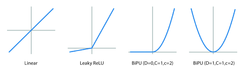
Figure 1.

Proof.

By taking $x=1$, we get $f(\lambda)=f(1)\lambda^{c}$ for any $\lambda>0$. Let $f(1)=C$. Then we see that for any $x>0$ we must have: $f(x)=Cx^{c}$. In addition, for every $\lambda>0$ we must have: $f(\lambda 0)=f(0)=\lambda^{c}f(0)$. So if $c=0$, then $f(x)=C=f(1)$ for $x\geq 0$. If $c\not=0$, then $f(0)=0$. In this case, if we want the activation function to be continuous, then we see that we must have $c\geq 0$. So in summary for $x>0$ we must have $f(x)=f(1)x^{c}=Cx^{c}$. For the function to be right continuous at 0, we must have either $f(0)=f(1)=C$ with $c=0$ or $f(0)=0$ with $c>0$. We can now look at negative values of $x$. By the same reasoning, we have $f(\lambda(-1))=f(-\lambda)=\lambda^{c}f(-1)$ for any $\lambda>0$. Thus for any $x<0$ we must have: $f(x)=f(-1)|x|^{c}=D|x|^{c}$ where $D=f(-1)$. Thus, if $f$ is continuous, there are two possibilities. If $c=0$, then we must have $C=f(1)=D(f-1)-$ and thus $f(x)=C$ everywhere. If $c\not=0$, then continuity requires that $c>0$. In this case $f(x)=Cx^{c}$ for $x\geq 0$ with $C=f(1)$, and $f(x)=Dx^{c}$ for $x<0$ with $f(-1)=D$. In all cases, it is easy to check directly that the resulting functions satisfy the functional equation given by Equation 6.3. ∎

6.2. Scaling BiPU Neurons

A BiPU neuron can be scaled by multiplying its incoming weight by $\lambda>0$ and dividing its outgoing weights by $1/\lambda^{c}$. This will not change the role of the corresponding unit in the network, and thus it will not change the input-output function of the network.

6.3. Balancing BiPU Neurons

As in the case of BiLU neurons, we balance a multiplicative neuron by asking what is the optimal scaling factor $\lambda$ that optimizes a particular regularizer. For simplicity, here we assume that the regularizer is in the $L_{p}$ class. Then we are interested in the value of $\lambda>0$ that minimizes the function:

$$\lambda^{p}\sum_{w\in IN}|w|^{p}+\frac{1}{\lambda^{pc}}\sum_{w\in OUT}|w|^{p}$$ (6.5)

A simple calculation shows that the optimal value of $\lambda$ is given by:

$$\lambda^{*}=\Bigl{(}\frac{c\sum_{OUT}|w|^{p}}{\sum_{IN}|w|^{p}}\Bigr{)}^{1/p(c+1)}$$ (6.6)

Thus after balancing the weights, the neuron must satisfy the balance equation:

$${c\sum_{OUT}|w|^{p}}=\sum_{IN}|w|^{p}$$ (6.7)

in the new weights $w$.

So far, we have focused on balancing individual neurons. In the next two sections, we look at balancing across all the units of a network. We first look at what happens to network balance when a network is trained by gradient descent and then at what happens to network balance when individual neurons are balanced iteratively in a regular or stochastic manner.

7. Network Balance: Gradient Descent

A natural question is whether gradient descent (or stochastic gradient descent) applied to a network of BiLU neurons, with or without a regularizer, converges to a balanced state of the network, where all the BiLU neurons are balanced. So we first consider the case where there is no regularizer (${\mathcal{E}}=E$). The results in [9] may suggest that gradient descent may converge to a balanced state. In particular, they write that for any neuron $i$:

$$\frac{d}{dt}\bigl{(}\sum_{w\in IN(i)}w^{2}-\sum_{w\in OUT(i)}w^{2}\bigr{)}=0$$ (7.1)

Thus the gradient flow exactly preserves the difference between the $L_{2}$ cost of the incoming and outgoing weights or, in other words, the derivative of the $L_{2}$ balance deficit is zero. Thus if one were to start from a balanced state and use an infinitesimally small learning rate one ought to stay in a balanced state at all times.

However, it must be noted that this result was derived for the $L_{2}$ metric only, and thus would not cover other $L_{p}$ forms of balance. Furthermore, it requires an infinitesimally small learning rate. In practice, when any standard learning rate is applied, we find that gradient descent does not converge to a balanced state (Figure 1). However, things are different when a regularizer term is included in the error functions as described in the following theorem.

Theorem 7.1.

Gradient descent in a network of BiLU units with error function ${\mathcal{E}}=E+R$ where $R$ has the properties described in Theorem 5.6 (including all $L_{p}$) must converge to a balanced state, where every BiLU neuron is balanced.

Proof.

By contradiction, suppose that gradient descent converges to a state that is unbalanced and where the gradient with respect to all the weights is zero. Then there is at least one unbalanced neuron in the network. We can then multiply the incoming weights of such a neuron by $\lambda$ and the outgoing weights by $1/\lambda$ as in the previous section without changing the value of $E$. Since the neuron is not in balance, we can move $\lambda$ infinitesimally so as to reduce $R$, and hence $\mathcal{E}$. But this contradicts the fact that the gradient is zero. ∎

Remark 7.2.

In practice, in the case of stochastic gradient descent applied to $E+R$, at the end of learning the algorithm may hover around a balanced state. If the state reached by the stochastic gradient descent procedure is not approximately balanced, then learning ought to continue. In other words, the degree of balance could be used to monitor whether learning has converged or not. Balance is a necessary, but not sufficient, condition for being at the optimum.

Remark 7.3.

If early stopping is being used to control overfitting, there is no reason for the stopping state to be balanced. However, the balancing algorithms described in the next section could be used to balance this state.

8. Network Balance: Stochastic or Deterministic Balancing Algorithms

In this section, we look at balancing algorithms where, starting from an initial weight configuration $W$, the BiLU neurons of a network are balanced iteratively according to some deterministic or stochastic schedule that periodically visits all the neurons. We can also include algorithms where neurons are partitioned into groups (e.g. neuronal layers) and neurons in each group are balanced together.

8.1. Basic Stochastic Balancing

The most interesting algorithm is when the BiLU neurons of a network are iteratively balanced in a purely stochastic manner. This algorithm is particularly attractive from the standpoint of physically implemented neural networks because the balancing algorithm is local and the updates occur randomly without the need for any kind of central coordination. As we shall see in the following section, the random local operations remarkably lead to a unique form of global order. The proof for the stochastic case extends immediately to the deterministic case, where the BiLU neurons are updated in a deterministic fashion, for instance by repeatedly cycling through them according to some fixed order.

8.2. Subset Balancing (Independent or Tied)

It is also possible to partition the BiLU neurons into non-overlapping subsets of neurons, and then balance each subset, especially when the neurons in each subset are disjoint of each other. In this case, one can balance all the neurons in a given subset, and repeat this subset-balancing operation subset-by-subset, again in a deterministic or stochastic manner. Because the BiLU neurons in each subset are disjoint, it does not matter whether the neurons in a given subset are updated synchronously or sequentially (and in which order). Since the neurons are balanced independently of each other, this can be called independent subset balancing. For example, in a layered feedforward network with no lateral connections, each layer corresponds to a subset of disjoint neurons. The incoming and outgoing connections of each neuron are distinct from the incoming and outgoing connections of any other neuron in the layer, and thus the balancing operation of any neuron in the layer does not interfere with the balancing operation of any other neuron in the same layer. So this corresponds to independent layer balancing,

As a side note, balancing a layer $h$, may disrupt the balance of layer $h+1$. However, balancing layer $h$ and $h+2$ (or any other layer further apart) can be done without interference of the balancing processes. This suggests also an alternating balancing scheme, where one alternatively balances all the odd-numbered layers, and all the evenly-numbered layers.

Yet another variation is when the neurons in a disjoint subset are tied to each other in the sense that they must all share the same scaling factor $\lambda$. In this case, balancing the subset requires finding the optimal $\lambda$ for the entire subset, as opposed to finding the optimal $\lambda$ for each neuron in the subset. Since the neurons are balanced in a coordinated or tied fashion, this can be called coordinated or tied subset balancing. For example, tied layer balancing must use the same $\lambda$ for all the neurons in a given layer. It is easy to see that this approach leads to layer synaptic balance which has the form (for an $L_{p}$ regularizer):

$$\sum_{i}\sum_{w\in IN(i)}|w|^{p}=\sum_{i}\sum_{w\in OUT(i)}|w|^{p}$$ (8.1)

where $i$ runs over all the neurons in the layer. This does not necessarily imply that each neuron in the layer is individually balanced. Thus neuronal balance for every neuron in a layer implies layer balance, but the converse is not true. Independent layer balancing will lead to layer balance. Coordinated layer balancing will lead to layer balance, but not necessarily to neuronal balance of each neuron in the layer. Layer-wise balancing, independent or tied, can be applied to all the layers and in deterministic (e.g. sequential) or stochastic manner. Again the proof given in the next section for the basic stochastic algorithm can easily be applied to these cases (see also Appendix B).

8.3. Remarks about Weight Sharing and Convolutional Neural Networks

Suppose that two connections share the same weight so that we must have: $w_{ij}=w_{kl}$ at all times. In general, when the balancing algorithm is applied to neuron $i$ or $j$, the weight $w_{ij}$ will change and the same change must be applied to $w_{kl}$. The latter may disrupt the balance of neuron $k$ or $l$. Furthermore, this may not lead to a decrease in the overall value of the regularizer $R$.

The case of convolutional networks is somewhat special, since all the incoming weights of the neurons sharing the same convolutional kernel are shared. However, in general, the outgoing weights are not shared. Furthermore, certain operations like max-pooling are not homogeneous. So if one trains a CNN with $E$ alone, or even with $E+R$, one should not expect any kind of balance to emerge in the convolution units. However, all the other BiLU units in the network should become balanced by the same argument used for gradient descent above. The balancing algorithm applied to individual neurons, or the independent layer balancing algorithm, will not balance individual neurons sharing the same convolution kernel. The only balancing algorithm that could lead to some convolution layer balance, but not to individual neuronal balance, is the coordinated layer balancing, where the same $\lambda$ is used for all the neurons in the same convolution layer, provided that their activation functions are BiLU functions.

We can now study the convergence properties of balancing algorithms.

9. Convergence of Balancing Algorithms

We now consider the basic stochastic balancing algorithm, where BiLU neurons are iteratively and stochastically balanced. It is essential to note that balancing a neuron $j$ may break the balance of another neuron $i$ to which $j$ is connected. Thus convergence of iterated balancing is not obvious. There are three key questions to be addressed for the basic stochastic algorithm, as well as all the other balancing variations. First, does the value of the regularizer converges to a finite value? Second, do the weights themselves converge to fixed finite values representing a balanced state for the entire network? And third, if the weights converge, do they always converge to the same values, irrespective of the order in which the units are being balanced? In other words, given an initial state $W$ for the network, is there a unique corresponding balanced state, with the same input-output functionalities?

9.1. Notation and Key Questions

For simplicity, we use a continuous time notation. After a certain time $t$ each neuron has been balanced a certain number of times. While the balancing operations are not commutative as balancing operations, they are commutative as scaling operations. Thus we can reorder the scaling operations and group them neuron by neuron so that, for instance, neuron $i$ has been scaled by the sequence of scaling operations:

$$S_{\lambda_{1}^{*}}(i)S_{\lambda_{2}^{*}}(i)\ldots S_{\lambda_{n_{it}}^{*}}(i)=S_{\Lambda_{i}(t)}(i)$$ (9.1)

where $n_{it}$ corresponds to the count of the last update of neuron $i$ prior to time $t$, and:

$$\Lambda_{i}(t)=\prod_{1\leq n\leq n_{it}}\lambda_{n}^{*}(i)$$ (9.2)

For the input and output units, we can consider that their balancing coefficients $\lambda^{*}$ are always equal to 1 (at all times) and therefore $\Lambda_{i}(t)=1$ for any visible unit $i$.

Thus, we first want to know if $R$ converges. Second, we want to know if the weights converge. This question can be split into two sub-questions: (1) Do the balancing factors $\lambda^{*}_{n}(i)$ converge to a limit as time goes to infinity. Even if the $\lambda^{*}_{n}(i)$’s converge to a limit, this does not imply that the weights of the network converge to a limit. After a time $t$, the weight $w_{ij}(t)$ between neuron $j$ and neuron $i$ has the value $w_{ij}\Lambda_{i}(t)/\Lambda_{j}(t)$, where $w_{ij}=w_{ij}(0)$ is the value of the weight at the start of the stochastic balancing algorithm. Thus: (2) Do the quantities $\Lambda_{i}(t)$ converge to finite values, different from 0? And third, if the weights converge to finite values different from 0, are these values unique or not, i.e. do they depend on the details of the stochastic updates or not? These questions are answered by the following main theorem..

9.2. Convergence of the Basic Stochastic Balancing Algorithm to a Unique Optimum

Theorem 9.1.

(Convergence of Stochastic Balancing) Consider a network of BiLU neurons with an error function ${\mathcal{E}}(W)=E(W)+R(W)$ where $R$ satisfies the conditions of Theorem 5.2 including all $L_{p}$ ($p>0$). Let $W$ denote the initial weights. When the neuronal stochastic balancing algorithm is applied throughout the network so that every neuron is visited from time to time, then $E(W)$ remains unchanged but $R(W)$ must converge to some finite value that is less or equal to the initial value, strictly less if the initial weights are not balanced. In addition, for every neuron $i$, $\lambda^{*}_{i}(t)\to 1$ and $\Lambda_{i}(t)\to\Lambda_{i}$ as $t\to\infty$, where $\Lambda_{i}$ is finite and $\Lambda_{i}>0$ for every $i$. As a result, the weights themselves must converge to a limit $W^{\prime}$ which is globally balanced, with $E(W)=E(W^{\prime})$ and $R(W)\geq R(W^{\prime})$, and with equality if only if $W$ is already balanced. Finally, $W^{\prime}$ is unique as it corresponds to the solution of a strictly convex optimization problem in the variables $L_{ij}=\log(\Lambda_{i}/\Lambda_{j})$ with linear constraints of the form $\sum_{\pi}L_{ij}=0$ along any path $\pi$ joining an input unit to an output unit and along any directed cycle (for recurrent networks). Stochastic balancing projects to stochastic trajectories in the linear manifold that run from the origin to the unique optimal configuration.

Proof.

Each individual balancing operation leaves $E(W)$ unchanged because the BiLU neurons are homogeneous. Furthermore, each balancing operation reduces the regularization error $R(W)$, or leaves it unchanged. Since the regularizer is lower-bounded by zero, the value of the regularizer must approach a limit as the stochastic updates are being applied.

For the second question, when neuron $i$ is balanced at some step, we know that the regularizer $R$ decreases by:

$$\Delta R=\biggl{(}\bigl{(}\sum_{w\in IN(i)}|w|^{p}\bigr{)}^{1/2}-\bigl{(}\sum_{w\in OUT(i)}|w|^{p}\bigr{)}^{1/2}\biggr{)}^{2}$$ (9.3)

If the convergence were to occur in a finite number of steps, then the coefficients $\lambda^{*}_{i}(t)$ must become equal and constant to 1 and the result is obvious. So we can focus on the case where the convergence does not occur in a finite number of steps (indeed this is the main scenario, as we shall see at the end of the proof). Since $\Delta R\to 0$, we must have:

$$\sum_{w\in IN(i)}|w|^{p}\to\sum_{w\in OUT(i)}|w|^{p}$$ (9.4)

But from the expression for $\lambda^{*}$ (Equation 5.14), this implies that for every $i$, $\lambda^{*}_{n}(i)\to 1$ as time increases ($n\to\infty$). This alone is not sufficient to prove that $\Lambda_{i}(t)$ converges for every $i$ as $t\to\infty$. However, it is easy to see that $\Lambda_{i}(t)$ cannot contain a sub-sequence that approaches 0 or $\infty$ (Figure 2). Furthermore, not only $\Delta R$ converges to 0, but the series $\sum\Delta R$ is convergent. This shows that, for every $i$, $\Delta_{i}(t)$ must converge to a finite, non-zero value $\Delta_{i}$. Therefore all the weights must converge to fixed values given by $w_{ij}(0)\Lambda_{i}/\Lambda_{j}$.

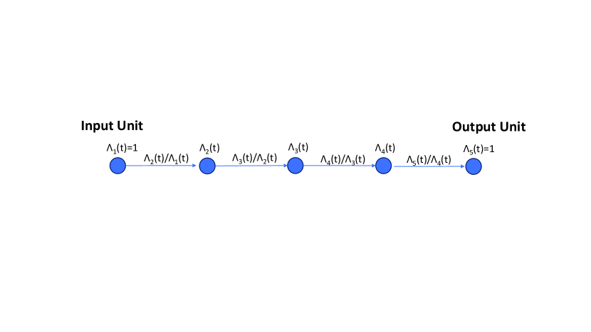
Figure 2. A path with three hidden BiLU units connecting one input unit to one output unit. During the application of the stochastic balancing algorithm, at time $t$ each unit $i$ has a cumulative scaling factor $\Lambda_{i}(t)$, and each directed edge from unit $j$ to unit $i$ has a scaling factor $M_{ij}(t)=\Lambda_{i}(t)/\Lambda_{j}(t)$. The $\lambda_{i}(t)$ must remain within a finite closed interval away from 0 and infinity. To see this, imagine for instance that there is a subsequence of $\Lambda_{3}(t)$ that approaches 0. Then there must be a corresponding subsequence of $\Lambda_{4}(t)$ that approaches 0, or else the contribution of the weight $w_{43}\Lambda_{4}(t)/\Lambda_{3}(t)$ to the regularizer would go to infinity. But then, as we reach the output layer, the contribution of the last weight $w_{54}\Lambda_{5}(t)/\Lambda_{4}(t)$ to the regularizer goes to infinity because $\Lambda_{5}(t)$ is fixed to 1 and cannot compensate for the small values of $\Lambda_{4}(t)$. And similarly, if there is a subsequence of $\Lambda_{3}(t)$ going to infinity, we obtain a contradiction by propagating its effect towards the input layer.

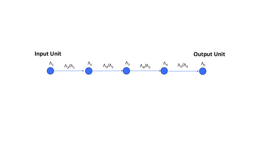
Figure 3. A path with five units. After the stochastic balancing algorithm has converged, each unit $i$ has a scaling factor $\Lambda_{i}$, and each directed edge from unit $j$ to unit $i$ has a scaling factor $M_{ij}=\Lambda_{i}/\Lambda_{j}$. The products of the $M_{ij}$’s along the path is given by: $\frac{\Lambda_{2}}{\Lambda_{1}}\frac{\Lambda_{3}}{\Lambda_{2}}\frac{\Lambda_{4}}{\Lambda_{3}}\frac{\Lambda_{5}}{\Lambda_{4}}=\frac{\Lambda_{5}}{\Lambda_{1}}$. Accordingly, if we sum the variables $L_{ij}=\log M_{ij}$ along the directed path, we get $L_{21}+L_{32}+L_{43}+L_{54}=\log\Lambda_{5}-\log\Lambda_{1}$. In particular, if unit 1 is an input unit and unit 5 is an output unit, we must have $\Lambda_{1}=\Lambda_{5}=1$ and thus: $L_{21}+L_{32}+L_{43}+L_{54}=0$. Likewise, in the case of a directed cycle where unit 1 and unit 5 are the same, we must have: $L_{21}+L_{32}+L_{43}+L_{54}+L_{15}=0$.

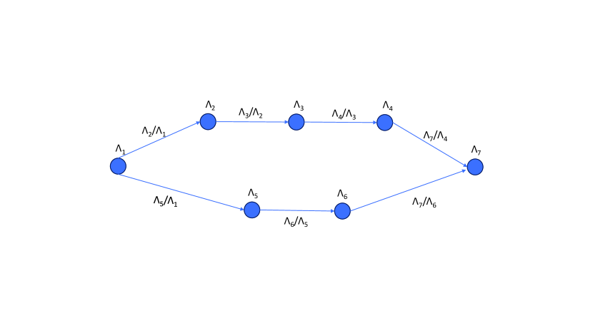
Figure 4. Two hidden units (1 and 7) connected by two different directed paths 1-2-3-4-7 and 1-5-6-7 in a BiLU network. Each unit $i$ has a scaling factor $\Lambda_{i}$, and each directed edge from unit $j$ to unit $i$ has a scaling factor $M_{ij}=\Lambda_{i}/\Lambda_{j}$. The products of the $M_{ij}$’s along each path is equal to: $\frac{\Lambda_{2}}{\Lambda_{1}}\frac{\Lambda_{3}}{\Lambda_{2}}\frac{\Lambda_{4}}{\Lambda_{3}}\frac{\Lambda_{7}}{\Lambda_{4}}=\frac{\Lambda_{5}}{\Lambda_{1}}\frac{\Lambda_{6}}{\Lambda_{5}}\frac{\Lambda_{7}}{\Lambda_{6}}=\frac{\Lambda_{7}}{\Lambda_{1}}$. Therefore the variables $L_{ij}=\log M_{ij}$ must satisfy the linear equation: $L_{21}+L_{32}+L_{43}+L_{74}=L_{51}+L_{65}+L_{76}$ =$\log\Lambda_{7}-\log\Lambda_{1}$.

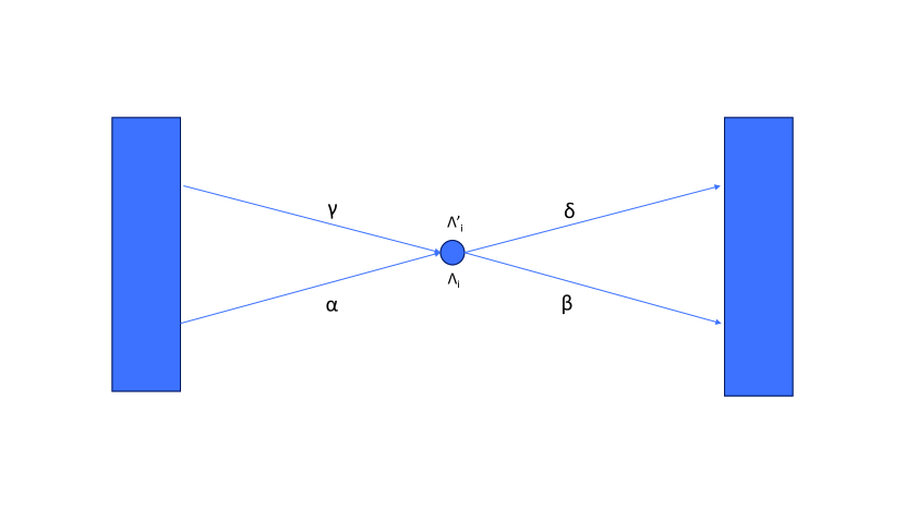
Figure 5. Consider two paths $\alpha+\beta$ and $\gamma+\delta$ from the input layer to the output layer going through the same unit $i$. Let us assume that the first path assigns a multiplier $\Lambda_{i}$ to unit $i$ and the second path assigns a multiplier $\Lambda^{\prime}_{i}$ to the same unit. By assumption we must have: $\sum_{\alpha}L_{ij}+\sum_{\beta}L_{ij}=0$ for the first path, and $\sum_{\gamma}L_{ij}+\sum_{\delta}L_{ij}=0$. But $\alpha+\delta$ and $\gamma+\beta$ are also paths from the input layer to the output layer and therefore: $\sum_{\alpha}L_{ij}+\sum_{\delta}L_{ij}=0$ and $\sum_{\gamma}L_{ij}+\sum_{\beta}L_{ij}=0$. As a result, $\sum_{\alpha}L_{ij}=\log\Lambda_{i}=\sum_{\gamma}L_{ij}=\Lambda^{\prime}_{i}$. Therefore the assignment of the multiplier $\Lambda_{i}$ must be consistent across different paths going through unit $i$.

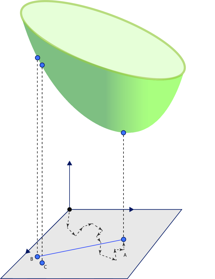
Figure 6. The problem of minimizing the strictly convex regularizer $R(L_{ij})=\sum_{ij}e^{pL_{ij}}|w_{ij}|^{p}$ ($p>0$), over the linear (hence convex) manifold of self-consistent configurations defined by the linear constraints of the form $\sum_{\pi}L_{ij}=0$, where $\pi$ runs over input-output paths. The regularizer function depends on the weights. The linear manifold depends only on the architecture, i.e., the graph of connections. This is a strictly convex optimization problem with a unique solution associated with the point $A$. At $A$ the corresponding weights must be balanced, or else a self-consistent configuration of lower cost could be found by balancing any non-balanced neuron. Finally, any other self-consistent configuration $B$ cannot correspond to a balanced state of the network, since there must exist balancing moves that further reduce the regularizer cost (see main text). Stochastic balancing produces random paths from the origin, where $L_{ij=}\log M_{ij}=0$, to the unique optimum point $A$.

Finally, we prove that given an initial set of weights $W$, the final balanced state is unique and independent of the order of the balancing operations. The coefficients $\Lambda_{i}$ corresponding to a globally balanced state must be solutions of the following optimization problem:

$$\min_{\Lambda}R(\Lambda)=\sum_{ij}|\frac{\Lambda_{i}}{\Lambda_{j}}w_{ij}|^{p}$$ (9.5)

under the simple constraints: $\Lambda_{i}>0$ for all the BiLU hidden units, and $\Lambda_{i}=1$ for all the visible (input and output) units. In this form, the problem is not convex. Introducing new variables $M_{j}=1/\Lambda_{j}$ is not sufficient to render the problem convex. Using variables $M_{ij}=\Lambda_{i}/\Lambda_{j}$ is better, but still problematic for $0<p\leq 1$. However, let us instead introduce the new variables $L_{ij}=\log(\Lambda_{i}/\Lambda_{j})$. These are well defined since we know that $\Lambda_{i}/\Lambda_{j}>0$. The objective now becomes:

$$\min R(L)=\sum_{ij}|e^{L_{ij}}w_{ij}|^{p}=\sum_{ij}e^{pL_{ij}}|w_{ij}|^{p}$$ (9.6)

This objective is strictly convex in the variables $L_{ij}$, as a sum of strictly convex functions (exponentials). However, to show that it is a convex optimization problem we need to study the constraints on the variables $L_{ij}$. In particular, from the set of $\Lambda_{i}$’s it is easy to construct a unique set of $L_{ij}$. However what about the converse?

Definition 9.2.

A set of real numbers $L_{ij}$, one per connection of a given neural architecture, is self-consistent if and only if there is a unique corresponding set of numbers $\Lambda_{i}>0$ (one per unit) such that: $\Lambda_{i}=1$ for all visible units and $L_{ij}=\log\Lambda_{i}/\Lambda_{j}$ for every directed connection from a unit $j$ to a unit $i$.

Remark 9.3.

This definition depends on the graph of connections, but not on the original values of the synaptic weights. Every balanced state is associated with a self-consistent set of $L_{ij}$, but not every self-consistent set of $L_{ij}$ is associated with a balanced state.

Proposition 9.4.

A set $L_{ij}$ associated with a neural architecture is self-consistent if and only if $\sum_{\pi}L_{ij}=0$ where $\pi$ is any directed path connecting an input unit to an output unit or any directed cycle (for recurrent networks).

Remark 9.5.

Thus the constraints associated with being a self-consistent configuration of $L_{ij}$’ s are all linear. This linear manifold of constraints depends only on the architecture, i.e., the graph of connections. The strictly convex function $R(L_{ij})$ depends on the actual weights $W$. Different sets of weights $W$ produce different convex functions over the same linear manifold.

Remark 9.6.

One could coalesce all the input units and all output units into a single unit, in which case a path from an input unit to and output unit becomes also a directed cycle. In this representation, the constraints are that the sum of the $L_{ij}$ must be zero along any directed cycle. In general, it is not necessary to write a constraint for every path from input units to output units. It is sufficient to select a representative set of paths such that every unit appears in at least one path.

Proof.

If we look at any directed path $\pi$ from unit $i$ to unit $j$, it is easy to see that we must have:

$$\sum_{\pi}L_{kl}=\log\Lambda_{i}-\log\Lambda_{j}$$ (9.7)

This is illustrated in Figures 3 and 4. Thus along any directed path that connects any input unit to any output unit, we must have $\sum_{\pi}L_{ij}=0$. In addition, for recurrent neural networks, if $\pi$ is a directed cycle we must also have: $\sum_{\pi}L_{ij}=0$. Thus in short we only need to add linear constraints of the form: $\sum_{\pi}L_{ij}=0$. Any unit is situated on a path from an input unit to an output unit. Along that path, it is easy to assign a value $\Lambda_{i}$ to each unit by simple propagation starting from the input unit which has a multiplier equal to 1. When the propagation terminates in the output unit, it terminates consistently because the output unit has a multiplier equal to 1 and, by assumption, the sum of the multipliers along the path must be zero. So we can derive scaling values $\Lambda_{i}$ from the variables $L_{ij}$. Finally, we need to show that there are no clashes, i.e. that it is not possible for two different propagation paths to assign different multiplier values to the same unit $i$. The reason for this is illustrated in Figure 5. ∎

We can now complete the proof Theorem 9.1. Given a neural network of BiLUs with a set of weights $W$, we can consider the problem of minimizing the regularizer $R(L_{ij}$ over the self-admissible configuration $L_{ij}$. For any $p>0$, the $L_{p}$ regularizer is strictly convex and the space of self-admissible configurations is linear and hence convex. Thus this is a strictly convex optimization problem that has a unique solution (Figure 6). Note that the minimization is carried over self-consistent configurations, which in general are not associated with balanced states. However, the configuration of the weights associated with the optimum set of $L_{ij}$ (point $A$ in Figure 6) must be balanced. To see this, imagine that one of the BiLU units–unit $i$ in the network is not balanced. Then we can balance it using a multiplier $\lambda_{i}^{*}$ and replace $\Lambda_{i}$ by $\Lambda_{i}^{\prime}=\Lambda_{i}\lambda^{*}$. It is easy to check that the new configuration including $\Lambda^{\prime}_{i}$ is self-consistent. Thus, by balancing unit $i$, we are able to reach a new self-consistent configuration with a lower value of $R$ which contradicts the fact that we are at the global minimum of the strictly convex optimization problem.

We know that the stochastic balancing algorithm always converges to a balanced state. We need to show that it cannot converge to any other balanced state, and in fact that the global optimum is the only balanced state. By contradiction, suppose it converges to a different balanced state associated with the coordinates $(L^{B}_{ij})$ (point $B$ in Figure 6). Because of the self-consistency, this point is also associated with a unique set of $(\Lambda^{B}_{i})$ coordinates. The cost function is continuous and differentiable in both the $L_{ij}$’s and the $\Lambda_{i}$’s coordinates. If we look at the negative gradient of the regularizer, it is non-zero and therefore it must have at least one non-zero component $\partial R/\partial\Lambda_{i}$ along one of the $\Lambda_{i}$ coordinates. This implies that by scaling the corresponding unit $i$ in the network, the regularizer can be further reduced, and by balancing unit $i$ the balancing algorithm will reach a new point ($C$ in Figure 6) with lower regularizer cost. This contradicts the assumption that $B$ was associated with a balanced stated. Thus, given an initial set of weights $W$, the stochastic balancing algorithm must always converge to the same and unique optimal balanced state $W^{*}$ associated with the self-consistent point $A$. A particular stochastic schedule corresponds to a random path within the linear manifold from the origin (at time zero all the multipliers are equal to 1, and therefore for any $i$ and any $j$: $M_{ij}=1$ and $L_{ij}=0$) to the unique optimum point $A$. ∎

Remark 9.7.

From the proof, it is clear that the same result holds also for any deterministic balancing schedule, as well as for tied and non-tied subset balancing, e.g., for layer-wise balancing and tied layer-wise balancing. In the Appendix, we provide an analytical solution for the case of tied layer-wise balancing in a layered feed-forward network.

Remark 9.8.

The same convergence to the unique global optimum is observed if each neuron, when stochastically visited, is favorably scaled rather than balanced, i.e., it is scaled with a factor that reduces $R$ but not necessarily minimizes $R$. Stochastic balancing can also be viewed as a form of EM algorithm where the E and M steps can be taken fully or partially.

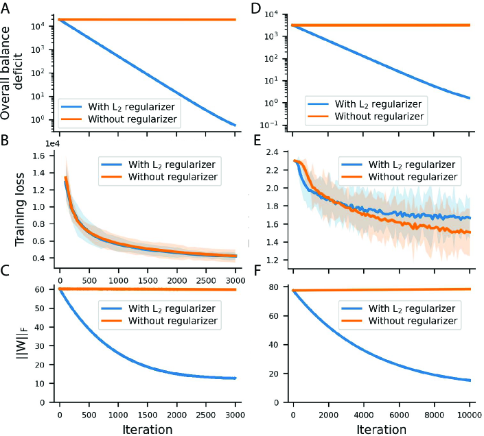
Figure 7. SGD applied to $E$ alone, in general, does not converge to a balanced state, but sGD applied to $E+R$ converges to a balanced state. (A-C) Simulations use a deep fully connected autoencoder trained on the MNIST dataset. (D-F) Simulations use a deep locally connected network trained on the CFAR10 dataset. (A,D) Regularization leads to neural balance. (B,E) The training loss decreases and converges during training (these panels are not meant for assessing the quality of learning when using a regularizer). (C,F) Using weight regularization decreases the norm of weights. (A-F) Shaded areas correspond to one s.t.d around the mean (in some cases the s.t.d. is small and the shaded area is not visible).

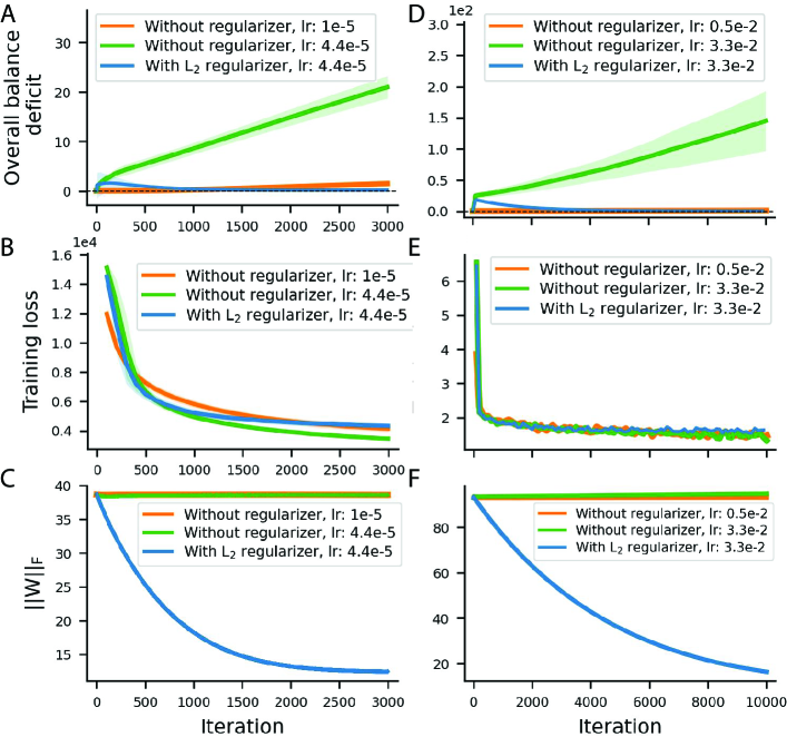
Figure 8. Even if the starting state is balanced, SGD does not preserve the balance unless the learning rate is infinitely small. (A-C) Simulations use a deep fully connected autoencoder trained on the MNIST dataset. (D-F) Simulations use deep locally connected network trained on the CFAR10 dataset. (A-F) The initial weights are balanced using the stochastic balancing algorithm. Then the network is trained by SGD. (A,D) When the learning rate (lr) is relatively large, without regularization, the initial balance of the network is rapidly disrupted. (B,E) The training loss decreases and converges during training (these panels are not meant for assessing the quality of learning when using a regularizer). (C,F) Using weight regularization decreases the norm of the weights. (A-F) Shaded areas correspond to one s.t.d around the mean (in some cases the s.t.d. is small and the shaded area is not visible).

10. Simulations

To further corroborate the results, we ran multiple experiments. Here we report the results from two series of experiments. The first one is conducted using a six-layer, fully connected, autoencoder trained on MNIST [8] for a reconstruction task with ReLU activation functions in all layers and the sum of squares errors loss function. The number of neurons in consecutive layers, from input to output, is 784, 200, 100, 50, 100, 200, 784. Stochastic gradient descent (SGD) learning by backpropagation is used for learning with a batch size of 200.

The second one is conducted using three locally connected layers followed by three fully connected layers trained on CFAR10 [18] for a classification task with leaky ReLU activation functions in the hidden layers, a softmax output layer, and the cross entropy loss function. The number of neurons in consecutive layers, from input to output, is 3072, 5000, 2592, 1296, 300, 100, 10. Stochastic gradient descent (SGD) learning by backpropagation is used for learning with a batch size of 5.

In all the simulation figures (Figures 7, 8, and 9) the left column presents results obtained from the first experiment, while the right column presents results obtained from the second experiment. While we used both $L_{1}$ and $L_{2}$ regularizers in the experiments, in the figures we report the results obtained with the $L_{2}$ regularizer, which is the most widely used regularizer. In Figures 7 and 8, training is done using batch gradient descent on the MNIST and CIFAR data. The balance deficit for a single neuron $i$ is defined as: $\bigl{(}\sum_{w\in IN(i)}w^{2}-\sum_{w\in OUT(i)}w^{2}\bigr{)}^{2}$, and the overall balance deficit is defined as the sum of these single-neuron balance deficits across all the hidden neurons in the network. The overall deficit is zero if and only if each neuron is in balance. In all the figures, $||W||_{F}$ denotes the Frobenius norm of the weights.

Figure 7 shows that learning by gradient descent with a $L_{2}$ regularizer results in a balanced state. Figure 8 shows that even when the network is initialized in a balanced state, without the regularizer the network can become unbalanced if the fixed learning rate is not very small. Figure 9 shows that the local stochastic balancing algorithm, by which neurons are randomly balanced in asynchronous fashion, always converges to the same (unique) global balanced state.

Code Availability: The code for reproducing the simulation results is available under the Apache 2.0 license at: https://github.com/ARahmansetayesh/a-theory-of-neural-synaptic-balance.

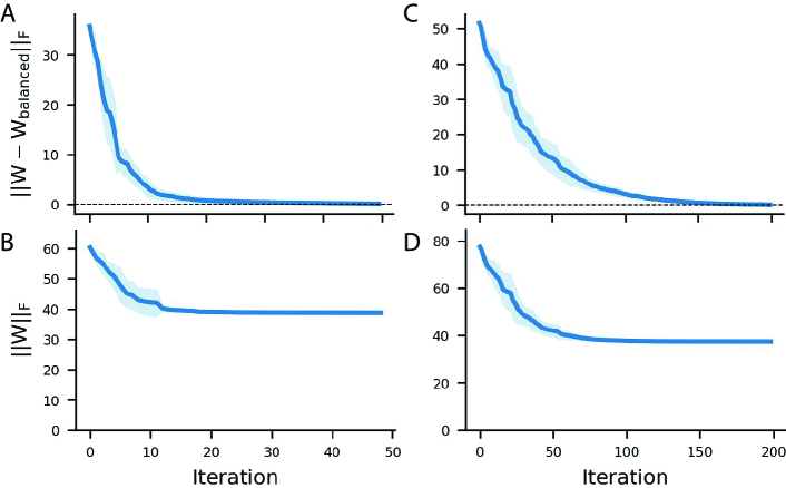
Figure 9. Stochastic balancing converges to a unique global balanced state (A-B) Simulations use a deep fully connected autoencoder trained on the MNIST dataset. (C-D) Simulations use deep locally connected network trained on the CFAR10 dataset. (A,C) The weights of the network are initialized randomly and saved. The stochastic balancing algorithm is applied and the resulting balanced weights are denoted by $W_{balanced}$. The stochastic balancing algorithm is applied 1,000 different times. In all repetitions, the weights converge to the same value $W_{balanced}$. (B,D) Stochastic balancing decreases the norm of the weights. (A-D) Shaded areas correspond to one standard deviation around the mean.

11. Discussion

While the theory of neural synaptic balance is a mathematical theory that stands on its own, it is worth considering some of its possible consequences and applications, at the theoretical, algorithmic, biological, and neuromorphic hardware levels.

11.1. Theory

Theories of deep learning in networks of McCulloch and Pitt neurons must often proceed by fixing the kinds of activation functions and neurons that are being used. At one extreme end of the spectrum, one finds linear networks for which a rich theory is available [3, 2]. At the other most non-linear end of the spectrum, one finds networks of unrestricted Boolean functions which are also amenable to fairly general analyses [1]. In between, one typically considers networks of linear threshold neurons [6], or sigmoidal neurons (logistic or tanh activation functions), or ReLU neurons [20]. The results shown here suggest that results obtained for networks of linear or ReLU neurons, may be exttendable to networks of BiLU neurons, especially when the homogeneity property plays an essential role, and perhaps also other neurons such as RePU neurons. In short, a line of investigation suggested by this work to study all the basic questions about deep learning (e.g. capacity, generalization, universal approximation properties) in networks of BiLU neurons of increasing architectural complexity. It is easy to show, for instance, that BiLU networks have universal approximation properties (see Appendix).

Our results show that for a given architecture with weights $W$, there is an entire equivalence class of weights with the same overall performance, associated with scaling operations and the underlying linear manifold. Global balancing can be viewed as a systematic way of selecting a unique canonical representative within the class, associated with the corresponding balanced network. Among other things, the existence of such equivalence classes implies that the information in the training data does not need to be able to specify the individual weights, but may instead specify the equivalence class of the weights. This is tied to the formal notion of capacity [6] and explain in part why large networks can be trained with less than $|W|$ examples while not overfitting [4]. It is worth noting that the equivalence classes corresponding to weights that provide the same input-output function may be even larger than what is given by the linear manifold of scalings, as they could contain other operations besides scaling, such as permuting the neurons of any given layer in the fully connected case. However, in the case of a feedforward network of BiLUs where the units are numbered, and connections run only from lower-numbered units to higher-numbered units, then each unit has its unique connectivity pattern and the equivalence classes may be restricted to scaling operations.

Another theoretical application is the study of learning in linear networks with $L_{p}$ regularization. For instance, it is well known that a feedforward, fully connected, linear autoencoder with bottleneck layers trained to minimize the sum of square reconstruction error $E$ has a unique global optimum, up to trivial transformations, corresponding to Principal Component Analysis (PCA) in the bottleneck layers. Furthermore, that problem has no spurious local minima and all other critical points of the error function are saddle points associated with projections onto linear spaces spanned by the non-principal components. What happens when an $L_{p}$ regularizer $R$ is added to the reconstruction error, so that the overall error is given by ${\ E}=E+\beta R$. For $\beta$ very large, $R$ will dominate and the optimal solution is to have all the weights equal to 0. However, when $\beta$ is small, the optimal solution is provided by the theory presented here. The error is dominated by $E$ so the optimum is associated with the PCA solution, as described above, which can then be refined by balancing to further reduce $R$ and reach the global optimum.

11.2. Algorithms

On the algorithmic side, we do not advocate that balancing algorithms should be used systematically, as SGD may reach balanced states by itself when applied with a regularizer, as we have seen in Section 7. Furthermore, balancing does not change the input-output function of a network and thus alone it cannot improve the performance of a network on the training or test sets. Nevertheless, balancing could be used at least: (1) to initialize a network in a balanced state prior to learning; (2) to check that a network trained to minimize $E+R$ has been properly trained by checking that each neuron is balanced with respect to $R$; (3) to balance a non-properly trained network; or (4) to tweak a network trained with ah $L_{p}$ regularization, towards a state where it is $L_{q}$ regularized (with $q\not=p$) without retraining it. It is also possible that periodically balancing a network during training may facilitate learning in some situations.

11.3. Biology

The balancing operations are local [5], in the sense that they involve only the pre-and post-synaptic weights of a neuron. Thus, unlike backpropagation, balancing is plausible in a physical neural system, as opposed to a digitally simulated neural system and conceivably balancing could be of interest in neuroscience or in neuromorphic engineering, for instance from the standpoint of learning or memory maintenance. While there is extensive literature in neuroscience on the balance between excitation and inhibition in biological networks [30, 26], there is no evidence in favor or against neuronal synaptic balance in the sense described here. However, there is some evidence for the existence of homeostatic processes that scale the input synaptic weights to regulate the activity of neurons [28, 7, 29]. In addition, there is also evidence that biological neurons can scale their intrinsic excitability (spike threshold) to regulate their activity [14, 11]. It is at least conceivable that these two scaling mechanisms could be at play and work together in some situations. In any case, current technology is quite far from allowing one to measure the strength of all the incoming and outgoing synapses of a biological neuron in an animal brain. Thus, it is impossible to draw any conclusions on the existence of some kind of homeostasis between the incoming and outgoing synapses of biological neurons. Exploratory experiments could potentially be carried either in simpler organisms with a small number of well-defined neurons, such as C. elegans, or in cultured neurons. Finally, simulations could be carried out in neural network models where inhibitory and excitatory neurons are segregated, possibly in uneven proportions–the overall ratio of excitatory to inhibitory neurons in the mammalian cortex is roughly 80% to 20% [21], with biologically-observed connectivity patterns.

11.4. Neuromorphic Hardware

In physical neural networks (e.g. biological neural networks, neuromorphic chips), as opposed to digitally simulated neural networks, the algorithms for adjusting synaptic weights must be local both in space and time. Yet these networks must exhibit good global properties. Thus, algorithms that are local and lead to global order, such as the balancing algorithms covered in this work, are of particular interest when considering physical, non-simulated, neural systems. For example, while a deep neuron embedded in a physical network may have no way of monitoring the global training error, conceivably it could sense and monitor its degree of balance, since that is an entirely local property. The degree of balance could be used as a local proxy to monitor global learning progress. Furthermore, the physical properties of the underlying hardware could constrain the synaptic weights or the learning algorithms in ways that could require or benefit from some form of neurall synaptic balance.

In particular, optimization strategies for training spiking neural networks with low energy consumption are analyzed in [24] (see also [22]). In particular, they explicitly mention the homogeneous properties of ReLU neurons and investigate how ReLU scaling can influence the number of spikes generated in each layer and the average energy consumption at each layer. Thus there is a direct connection between our work and some of the neuromorphic literature using scaling methods to control spiking rates and energy consumption, and this connection leads to a new questions for future work: how does balancing affects spiking neurons and energy consumption? Under which hardware conditions does balancing leads to optimal energy consumption?

An interesting special case is provided by memristor devices where the output voltage of neurons is calculated using the equation $V^{o}=V^{i}*GRs$ (see Figure 4 in [15]). In this equation $V^{i}$ is the presynaptic spike voltage, $G$ represents the memristor’s conductance (equivalent to synaptic weights), and $Rs$ is the output resistance of the postsynaptic neuron. The power consumption of the memristor is $(V^{i})^{2})G$, so the lower the value of $G$ is, the lower the power consumption of the memristor and minimizing the $L_{2}$ norm is directly connected to minimizing power consumption. Since our balancing algorithm is aimed precisely at minimizing the $L_{2}$ penalty), this establishes a direct connection between neural balance and energy minimization in memristor-based neuromorphic hardware. Moreover, the issue of the limited conductivity range of memristors is mentioned in [15] and in [16] Therefore, reducing the norm of the weights can help mitigate this issue as well.

12. Conclusion

The theory of neural synaptic balance explains some basic findings regarding $L_{2}$ balance in feedforward networks of ReLU neurons and extends them in several directions. The first direction is the extension to BiLU and other activation functions (BiPU). The second direction is the extension to more general regularizers, including all $L_{p}$ ($p>0$) regularizers. The third direction is the extension to non-layered architectures, recurrent architectures, convolutional architectures, as well as architectures with mixed activation functions. The theory is based on two local neuronal operations: scaling which is commutative, and balancing which is not commutative. Finally, and most importantly, given any initial set of weights, when local balancing operations are applied in a stochastic or deterministic manner, global order always emerges through the convergence of the balancing algorithm to the same unique set of balanced weights. The reason for this convergence is the existence of an underlying convex optimization problem where the relevant variables are constrained to a linear, only architecture-dependent, manifold. Scaling and balancing operations are local and thus may have applications in physical, non-digitally simulated, neural networks where the emergence of global order from local operations may lead to better operating characteristics and lower energy consumption.

Appendix A: Universal Approximation Properties of BiLU Neurons

Here we show that any continuous real-valued function defined over a compact set of the Euclidean space can be approximated to any degree of precision by a network of BiLU neurons with a single hidden layer. As in the case of the similar proof given in [2] using linear threshold gates in the hidden layer, it is enough to prove the theorem for a continuous function $f$: ${0,1}\to\mathbb{R}$.

Theorem 12.1.

(Universal Approximation Properties of BiLU Neurons) Let $f$ be any continuous function from $[0,1]$ to $\mathbb{R}$ and $\epsilon>0$. Let $g_{\lambda}$ be the ReLU activation function with slope $\lambda\in\mathbb{R}$s. Then there exists a feedforward network with a single hidden layer of neurons with ReLU activations of the form $g_{\lambda}$ and a single output linear neuron, i.e., with BiLU activation equal to the identity function, capable of approximating $f$ everywhere within $\epsilon$ (sup norm).

Proof.

To be clear, $g_{\lambda}(x)=0$ for $x<0$ and $g_{\lambda}(x)=\lambda x$ for $0\leq x$. Since $f$ is continuous over a compact set, it is uniformly continuous. Thus there exists $\alpha>0$ such that for any $x_{1}$ and $x_{2}$ in the $[0,1]$ interval:

$$|x_{2}-x_{1}|<\alpha\implies|f(x_{2})-f(x_{1})|<\epsilon\$$ (12.1)

Let $N$ be an integer such that $1<N\alpha$, and let us slice the interval $[0,1]$ into $N$ consecutive slices of width $h=1/N$, so that within each slice the function $f$ cannot jump by more than $\epsilon$. Let us connect the input unit to all the hidden units with a weight equal to 1. Let us have $N$ hidden units numbered $1,\ldots,N$ with biases equal to $0,1/N,2/N,....,N_{1}/N$ respectively and activation function of the form $g_{\lambda_{k}}$. It is essential that different units be allowed to have different slopes $\lambda_{k}$. The input unit is connected to all the hidden units and all the weights on these connections are equal to 1. Thus when $x$ is in the $k$-th slice, $(k-1)/N\leq x<k/N$, all the units from $k+1$ to $N$ have an output equal to $0$, and all the units from 1 to $k$ have an output determined by the corresponding slopes. All the hidden units are connected to the output unit with weights $\beta_{1},\ldots,\beta_{N}$, and $\beta_{0}$ is the bias of the output unit. We want the output unit to be linear. In order for the $\epsilon$ approximation to be satisfied, it is sufficient if in the $(k-1)/N\leq x<k/N$ interval, the output is equal to the line joining the point $f((k-1)/N)$ to the point $f(k/N)$. In other words, if $x\in[(k-1)/N,k/N)$, then we want the output of the network to be:

$$\beta_{0}+\sum_{i=1}^{k}\beta_{i}\lambda_{i}(x-(i-1)h)=f(\frac{k-1}{N})+\frac{f(\frac{k}{N})-f(\frac{k-1}{N})}{h}(x-(k-1)h)$$ (12.2)

By equating the y-intercept and slope of the lines on the left-hand side and the righ- hand side of Equation 12.2, we can solve for the weights $\beta$’s and the slopes $\lambda$’s. ∎

As in the case of the similar proof using linear threshold functions in the hidden layer (see [2],) this proof can easily be adapted to continuous functions defined over a compact set of $\mathbb{R}^{n}$, even with a finite number of finite discontinuities, and into $\mathbb{R}^{m}$.

Appendix B: Analytical Solution for the Unique Global Balanced State

Here we directly prove the convergence of stochastic balancing to a unique final balanced state, and derive the equations for the balanced state, in the special case of tied layer balancing (as opposed to single neuron balancing). The Proof and the resulting equations are also valid for stochastic balancing (one neuron at a time) in a layered architecture comprising a single neuron per layer. Let us call tied layer scaling the operation by which all the incoming weights to a given layer of BiLU neurons are multiplied by $\lambda>0$ and all the outgoing weights of the layer are multiplied by $1/\lambda$, again leaving the training error unchanged. Let us call layer balancing the particular scaling operation corresponding to the value of $\lambda$ that minimizes the contribution of the layer to the $L_{2}$ (or any other $L_{p}$) regularizer vaue. This optimal value of $\lambda^{*}$ results in layer-wise balance equations: the sum of the squares of all the incoming weights of the layer must be equal to the sum of the squares of all the outgoing weights of the layer in the $L_{2}$ case, and similarly in all $L^{P}$ cases.

Theorem 12.2.

Assume that tied layer balancing is applied iteratively and stochastically to the layers of a layered feedforward network of BiLU neurons. As long as all the layers are visited periodically, this procedure will always converge to the same unique set of weights, which will satisfy the layer-balance equations at all layers, irrespective of the details of the schedule. Furthermore, the balance state can be solved analytically.

Proof.

Every time a layer balancing operation is applied, the training error remains the same, and the $L_{2}$ (or any other $L_{p}$) regularization error decreases or stays the same. Since the regularization error is always positive, it must converge to a certain value. Using the same arguments as in the proof of Theorem 9.1, the weights must also converge to a stable configuration, and since the configuration is stable all its layers must satisfy the layer-wise balance equation. The key remaining question is why is this configuration unique and can we solve it analytically? Let $A_{1},A_{2},\ldots A_{N}$ denote the matrices of connections between the layers of the network. Let $\Lambda_{1},\Lambda_{2},\ldots,\Lambda_{N-1}$ be $N-1$ strictly positive multipliers, representing the limits of the products of the corresponding $\lambda_{i}^{*}$ associated with each balancing step at layer $i$, as in the proof of Theorem 9.1. In this notation, layer 0 is the input layer and layer $N$ is the output layer (with $\Lambda_{0}=1$ and $\Lambda_{N}=1$).

After converging, each matrix $A_{i}$ becomes the matrix $\Lambda_{i}/\Lambda_{i-1}A_{i}=M_{i}A_{i}$ for $i=1\ldots N$, with $M_{i}=\lambda_{i}/\Lambda_{i-1}$. The multipliers $M_{i}$ must minimize the regularizer while satisfying $M_{1}\ldots M_{N}=1$ to ensure that the training error remains unchanged. In other words, to find the values of the $M_{i}$’s we must minimize the Lagrangian:

$${\mathcal{L}}(M_{1},\ldots,M_{N})=\sum_{i=1}^{N}||M_{i}A_{i}||^{2}+\mu(1-\prod_{i=1}^{N}M_{i})$$ (12.3)

written for the $L^{2}$ case in terms of the Frobenius norm, but the analysis is similar in the general $L_{p}$ case. From this, we get the critical equations:

$$\frac{\partial{\mathcal{L}}}{\partial M_{i}}=2M_{i}||A_{i}||^{2}-\mu M_{1}\ldots M_{i-1}M_{i+1}\ldots M_{N}=0\quad{\rm for}\;i=1,\ldots,N\quad{\rm and}\quad\prod_{i=1}^{N}M_{i}=1$$ (12.4)

As a resut, for every $i$:

$$2M_{i}||A_{i}||^{2}-\frac{\mu}{M_{i}}=0\quad{\rm or}\quad\mu=2M_{i}^{2}||A_{i}||^{2}$$ (12.5)

Thus each $M_{i}>0$ can be expressed in a unique way as a function of the Lagrangian multiplier $\mu$ as: $M_{i}=(\mu/2||A_{i}||^{2})^{1/2}$. By writing again that the product of the $M_{i}$is equal to 1, we finally get:

$$\mu^{N}=2^{N}\prod_{i=1}^{N}||A_{i}||^{2}\quad{\rm or}\quad\mu=2\prod_{i=1}^{N}||A_{i}||^{2/N}$$ (12.6)

Thus we can solve for $M_{i}$:

$$M_{i}=\frac{\mu}{2||A_{i}||^{2}}=\frac{\prod_{i=1}^{N}||A_{i}||^{2/N}}{||A_{i}||^{2}}\quad\quad{\rm for}\;\;i=1,\ldots,N$$ (12.7)

Thus, in short, we obtain a unique closed-form expression for each $M_{i}$. From there, we infer the unique and final state of the weights, where $A^{*}_{i}=M_{i}A_{i}=\Lambda_{i}A_{l}/\Lambda_{l-1}$. Note that each $M_{i}$ depends on all the other $M_{j}$’s, again showcasing how the local balancing algorithm leads to a unique global solution. ∎

References

- [1] P. Baldi. Autoencoders, Unsupervised Learning, and Deep Architectures. Journal of Machine Learning Research. Proceedings of 2011 ICML Workshop on Unsupervised and Transfer Learning, 27:37–50, 2012.
- [2] P. Baldi. Deep Learning in Science. Cambridge University Press, Cambridge, UK, 2021.
- [3] P. Baldi and K. Hornik. Neural networks and principal component analysis: Learning from examples without local minima. Neural Networks, 2(1):53–58, 1989.
- [4] Pierre Baldi. Deep learning over-parameterization: the shallow fallacy. In Northern Lights Deep Learning Conference, pages 7–12. Proceedings Machine Learning Research, 2024.
- [5] Pierre Baldi and Peter Sadowski. A theory of local learning, the learning channel, and the optimality of backpropagation. Neural Networks, 83:61–74, 2016.
- [6] Pierre Baldi and Roman Vershynin. The capacity of feedforward neural networks. Neural Networks, 116:288–311, 2019. Also: arXiv preprint arXiv:1901.00434.
- [7] Marina Chistiakova, Nicholas M Bannon, Jen-Yung Chen, Maxim Bazhenov, and Maxim Volgushev. Homeostatic role of heterosynaptic plasticity: models and experiments. Frontiers in computational neuroscience, 9:89, 2015.
- [8] Li Deng. The mnist database of handwritten digit images for machine learning research. IEEE Signal Processing Magazine, 29(6):141–142, 2012.
- [9] Simon S Du, Wei Hu, and Jason D Lee. Algorithmic regularization in learning deep homogeneous models: Layers are automatically balanced. Advances in Neural Information Processing Systems, 31, 2018.
- [10] Rachel E Field, James A D’amour, Robin Tremblay, Christoph Miehl, Bernardo Rudy, Julijana Gjorgjieva, and Robert C Froemke. Heterosynaptic plasticity determines the set point for cortical excitatory-inhibitory balance. Neuron, 106(5):842–854, 2020.
- [11] Bertrand Fontaine, José Luis Peña, and Romain Brette. Spike-threshold adaptation predicted by membrane potential dynamics in vivo. PLoS computational biology, 10(4):e1003560, 2014.
- [12] Robert C Froemke. Plasticity of cortical excitatory-inhibitory balance. Annual review of neuroscience, 38:195–219, 2015.
- [13] Oliver D Howes and Ekaterina Shatalina. Integrating the neurodevelopmental and dopamine hypotheses of schizophrenia and the role of cortical excitation-inhibition balance. Biological psychiatry, 2022.
- [14] Chao Huang, Andrey Resnik, Tansu Celikel, and Bernhard Englitz. Adaptive spike threshold enables robust and temporally precise neuronal encoding. PLoS computational biology, 12(6):e1004984, 2016.
- [15] Dmitry Ivanov, Aleksandr Chezhegov, Mikhail Kiselev, Andrey Grunin, and Denis Larionov. Neuromorphic artificial intelligence systems. Frontiers in Neuroscience, 16:1513, 2022.
- [16] Yu Ji, YouHui Zhang, ShuangChen Li, Ping Chi, CiHang Jiang, Peng Qu, Yuan Xie, and WenGuang Chen. Neutrams: Neural network transformation and co-design under neuromorphic hardware constraints. In 2016 49th Annual IEEE/ACM International Symposium on Microarchitecture (MICRO), pages 1–13. IEEE, 2016.
- [17] Dongshin Kim and Jang-Sik Lee. Neurotransmitter-induced excitatory and inhibitory functions in artificial synapses. Advanced Functional Materials, 32(21):2200497, 2022.
- [18] Alex Krizhevsky and Geoffrey Hinton. Learning multiple layers of features from tiny images. 2009.
- [19] Behnam Neyshabur, Ryota Tomioka, Ruslan Salakhutdinov, and Nathan Srebro. Data-dependent path normalization in neural networks. arXiv preprint arXiv:1511.06747, 2015.
- [20] Philipp Petersen and Felix Voigtlaender. Optimal approximation of piecewise smooth functions using deep relu neural networks. Neural Networks, 108:296–330, 2018.
- [21] JLR Rubenstein and Michael M Merzenich. Model of autism: increased ratio of excitation/inhibition in key neural systems. Genes, Brain and Behavior, 2(5):255–267, 2003.
- [22] Bodo Rueckauer, Iulia-Alexandra Lungu, Yuhuang Hu, Michael Pfeiffer, and Shih-Chii Liu. Conversion of continuous-valued deep networks to efficient event-driven networks for image classification. Frontiers in neuroscience, 11:294078, 2017.
- [23] Farshad Shirani and Hannah Choi. On the physiological and structural contributors to the dynamic balance of excitation and inhibition in local cortical networks. bioRxiv, pages 2023–01, 2023.
- [24] Martino Sorbaro, Qian Liu, Massimo Bortone, and Sadique Sheik. Optimizing the energy consumption of spiking neural networks for neuromorphic applications. Frontiers in neuroscience, 14:662, 2020.
- [25] Christopher H Stock, Sarah E Harvey, Samuel A Ocko, and Surya Ganguli. Synaptic balancing: A biologically plausible local learning rule that provably increases neural network noise robustness without sacrificing task performance. PLOS Computational Biology, 18(9):e1010418, 2022.
- [26] Roberta Tatti, Melissa S Haley, Olivia K Swanson, Tenzin Tselha, and Arianna Maffei. Neurophysiology and regulation of the balance between excitation and inhibition in neocortical circuits. Biological psychiatry, 81(10):821–831, 2017.
- [27] A. Tavakoli, F. Agostinelli, and P. Baldi. SPLASH: Learnable activation functions for improving accuracy and adversarial robustness. Neural Networks, 140:1–12, 2021. Also: arXiv:2006.08947.
- [28] Gina Turrigiano. Homeostatic synaptic plasticity: local and global mechanisms for stabilizing neuronal function. Cold Spring Harbor perspectives in biology, 4(1):a005736, 2012.
- [29] Gina G Turrigiano. The dialectic of hebb and homeostasis. Philosophical transactions of the royal society B: biological sciences, 372(1715):20160258, 2017.
- [30] Carl Van Vreeswijk and Haim Sompolinsky. Chaos in neuronal networks with balanced excitatory and inhibitory activity. Science, 274(5293):1724–1726, 1996.