Electron heating in high Mach number collisionless shocks
Abstract
The energy partition in high Mach number collisionless shock waves is central to a wide range of high-energy astrophysical environments. We present a new theoretical model for electron heating that accounts for the energy exchange between electrons and ions at the shock. The fundamental mechanism relies on the difference in inertia between electrons and ions, resulting in differential scattering of the particles off a decelerating magnetically-dominated microturbulence across the shock transition. We show that the self-consistent interplay between the resulting ambipolar-type electric field and diffusive transport of electrons leads to efficient heating in the magnetic field produced by the Weibel instability in the high-Mach number regime and is consistent with fully kinetic simulations.
High Mach number collisionless shocks shape the electromagnetic signatures of many astrophysical environments. From pc-scale young supernovae remnants to Mpc-scale virial rings of galaxy clusters, the emission relies on the efficient acceleration of electrons and ions to highly relativistic speeds at the interface between a supersonic flow and a weakly magnetized plasma. The injection of electrons into acceleration processes [1, 2, 3, 4, 5, 6] and the interpretation of observations [7, 8, 9] directly depend on the electron heating efficiency and properties. The mechanisms that underpin the energy transfer and the temperature ratio between electrons and ions thus constitute one of the most fundamental open questions in our understanding of these blast waves.
Left as a free parameter from the Rankine-Hugoniot jump conditions, the electron-to-ion temperature ratio is inferred via various observational probes [10, 11], from radio and X-ray synchrotron emissions within young Supernova Remnant (SNR) shocks () [12] to in-situ measurements at Earth’s bow shock () [13]. The latter allowed for direct characterization of the shock dynamics with essential results on the structure gleaned from the Magnetospheric Multi-Scale (MMS) spacecraft [14], but the direct characterization of the temperature ratio for remains elusive. In parallel, rapid developments in high-power lasers, such as at OMEGA and the National Ignition Facility, are opening valuable opportunities to investigate high-Mach number collisionless shocks in controlled laboratory experiments for direct measurement of particle energization processes [15, 16, 17, 18].
These observational and experimental studies are supported by significant joint numerical efforts to self-consistently model the shock dynamics through multi-dimensional kinetic simulations, providing a detailed characterization of the plasma processes at play over limited timescales. These simulations cover various regimes of magnetosonic Mach numbers [19, 20, 21, 22, 23, 24, 25, 26, 27, 28, 29]. Despite all these substantial efforts, identifying and modeling the dominant source of electron heating in high magnetosonic Mach number shocks remains a critical challenge.
In this Letter, we present a model for electron transport and heating in self-generated microturbulence that can accurately capture the electron-ion temperature ratio observed in fully kinetic simulations of high-Mach number shocks. The generality of the approach presented here opens new avenues for modeling energy partition in systems governed by magnetically dominated turbulence.
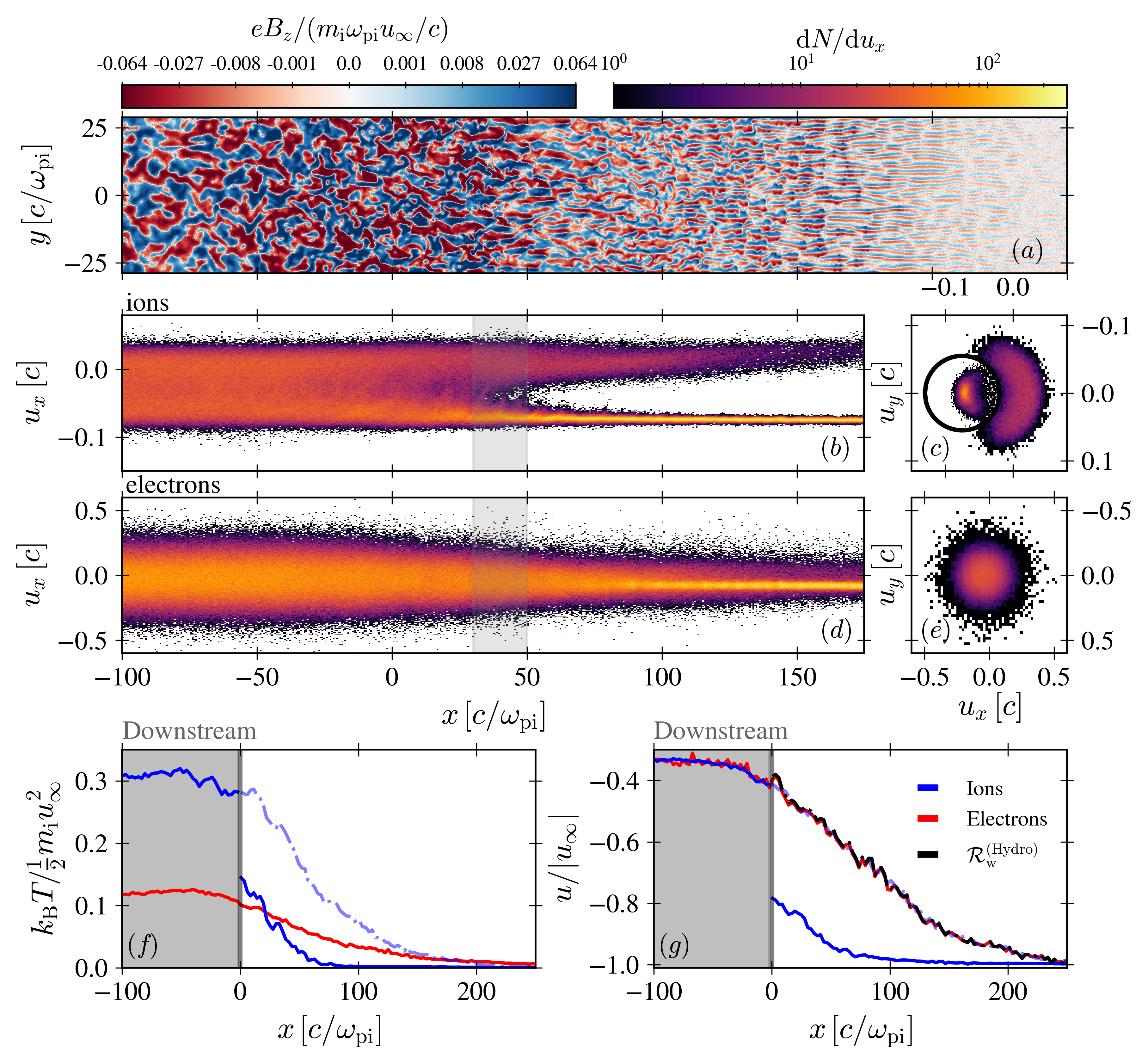
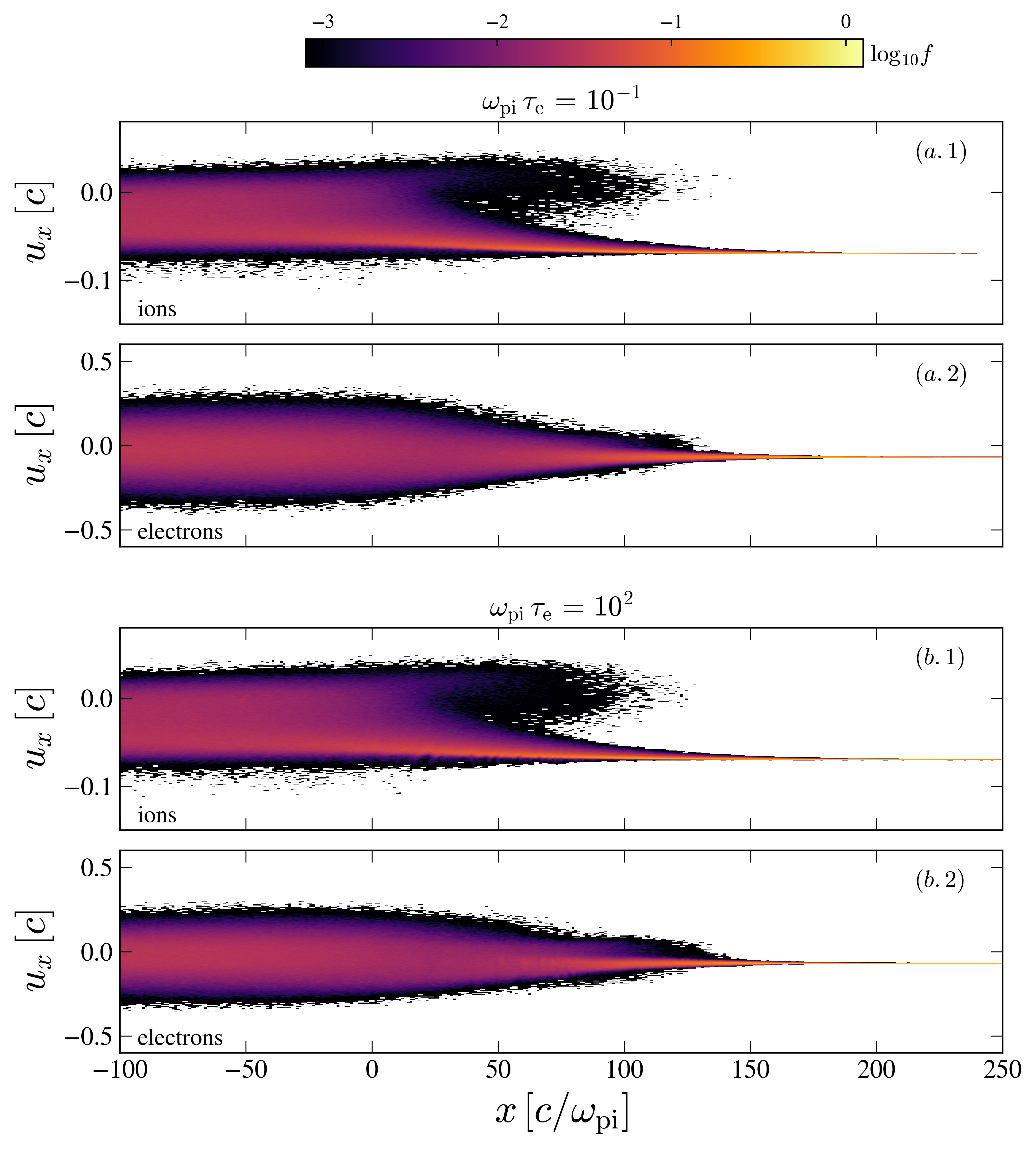
We start by analyzing the typical structure of high-Mach number collisionless shocks from the results of large-scale fully-kinetic plasma simulations, which can self-consistently capture the dynamics of shock formation and particle heating. We have performed a series of 2D particle-in-cell (PIC) simulations with the relativistic electromagnetic code TRISTAN-MP [30]. We initialize an electron-ion plasma at rest and set the left reflecting and conducting wall of our simulation box in motion along . The interaction between the reflected beam and the stationary plasma results in the formation of a shock. Our simulations are performed in the upstream frame. All quantities are then transformed and presented in the shock-front frame. A moving injector gradually recedes from the left wall at the speed of light. Space and time coordinates are normalized to the ion plasma skin depth and frequency , with the proper upstream density. We adopt a resolution of cells per electron skin depth, , and the timestep is = . In each direction, we use 32 particles per cell (ppc) and filter the current 32 times per timestep [30]. We tested convergence varying ppc , , and , where is the far upstream velocity in the shock front frame (see Supplemental Material [31]).
As a reference for the following discussion, we consider a non-relativistic shock in the limit of very high Alfvén Mach number, i.e., initially unmagnetized, with , , and upstream ion temperature . The results of the simulation are illustrated in Fig. 1, where we zoom in on the shock structure and precursor region. We observe that the interaction between the shock-reflected hot beam of ions propagating at positive velocity and the incoming upstream plasma drives a microturbulence via the Weibel, or current-filamentation, instability [32, 33] (Fig.1a) and leads to efficient electron heating (Fig.1f-g) to an electron-to-ion temperature ratio of . Qualitatively, our model captures the deceleration of the turbulence across the shock and the associated charge separation between species of different inertia. Electrons accelerate in the coherent electrostatic field that ensues and isotropize over their short scattering time scale through fast decoherence of the betatron motion. This diffusive process leads to efficient energy channeling between electrons and ions.
The microturbulence is magnetically dominated, so the scalar everywhere in the shock precursor and downstream. This means one can always find a frame, , in which the electric field component vanishes locally. This frame drifts at a velocity in the shock front frame. For statistically homogeneous turbulence transverse to the shock normal, the instantaneous velocity of this frame, , is a function of the longitudinal -coordinate only. The scattering center frame extracted from the fully hydrodynamic limit [34] shows good agreement of the average proper motion of nonlinear structures, close to the electron drift velocity (Fig.1g). Ions from the backstreaming beam can be differentiated from the background — i.e., incoming upstream flow — via a threshold set at (Fig.1c). Across the shock transition, does not coincide with the drift velocity of the background ions (Fig.1g) and is, therefore, non-ideal. Motivated by these observations, we explore a theoretical description of electron transport and heating in high-Mach number shocks to model the fraction of incoming energy density imparted to the electron distribution.
The equation of motion for a single charged particle in a non-inertial frame reads , where the first term accounts for pitch-angle variation in , the second term accounts for acceleration by the longitudinal electric field , and the last term for the non-inertial nature of . This approach offers a natural way to disentangle the contribution of the motional and electrostatic electric fields. If one defines as a random force with the stochastic variables encoded in the form of the rotation matrix and keeps a self-consistent -field contribution, the above equation of motion reduces to a semi-dynamical model of transport in a Langevin equation [35].
At this stage, the electric field contribution and origin are still unclear. Following the same arguments as in [36, 34, 37], we assume that the variation timescale of the turbulent structures is much larger than the typical scattering time of the electrons off these quasi-magnetostatic structures. Therefore, we neglect the contribution of the inductive electric field from the linear growth of plasma instabilities. We constrain the electric field to be electrostatic and build a reduced description for electron heating along those lines. The broadband longitudinal and transverse spectra of Weibel modes excited in the shock precursor, coupled with the nontrivial contributions of other channels such as the definition of and , make the statistical description of challenging to compare with fully kinetic simulations. The simplest nontrivial approximation assumes an isotropic Gaussian white noise process where is a linear combination of the generators of the rotation group corresponding to pitch-angle scattering in the turbulent magnetic field [38]. Based on these assumptions, we now aim at deriving a self-consistent relation for the electrostatic coupling between electrons and ions.
In this limit, the stochastic differential equation of motion is equivalent to a transport equation for the particle distribution for the species . In the shock-front frame, where the system is assumed stationary, the transport equation reads:
| (1) |
where the right-hand side is the operator for elastic scattering in in 3D with the pitch-angle cosine and is the scattering frequency [39]. For a two-dimensional distribution, the operator reduces to . In the nonrelativistic regime, the Larmor radius of electrons remains small compared to the size of the scattering centers. The scattering center frame and the electron bulk velocity are, therefore, drifting at similar speeds (Fig.1g). In this diffusive limit, the distribution function can be expanded in Legendre polynomials . Averaging Eq. (I) over the first two Legendre polynomials and assuming a dominant contribution from the electric field, we obtain a kinetic closure for the Fokker-Planck equation accounting for momentum diffusion in the electrostatic fields [31]:
| (2) |
The right-hand side only accounts for the dominant term responsible for the bulk heating of the electrons. This term predicts heating proportional to the diffusion coefficient 111An analogous form was obtained in [1] for the noninertial contribution uniquely and in [37, 54] in the respective relativistic regimes of collisionless and radiation-mediated blast waves. .
Based on this picture, the development of a coherent electric field across the shock transition leads to electron stochastic heating. However, the origin of this electric field is not explicit. With a rate proportional to the square of the field amplitude, the heating mechanism we describe is similar to Joule heating from ambipolar diffusion. The decelerating scattering centers effectively act as a neutral species on which electrons and ions elastically scatter at different rates. An ambipolar electric field ensues from the larger effective frictional drag of the decelerating microturbulence on the electrons relative to the ions, leading to efficient diffusive heating of the electrons in a Joule process.
To capture the ambipolar nature of electron heating and the self-consistent coupling between electrons and ions, we combine a Monte Carlo (MC) method with a Poisson (MC-P) solver to achieve a complete solution of the transport equation [41]. We use a resolution , , -order spline interpolation between particles and -field, with isotropic white noise statistics for pitch-angle scattering. Electrons and ions are injected from the right-hand side of the domain with an initial bulk velocity and a temperature matching the initial conditions of PIC simulations. For a fair comparison with PIC simulation, we used a 2D scattering operator. Comparison between 2D and generalized 3D scattering operators showed no significant differences up to realistic mass ratios. Using our solver, we recover the Rankine-Hugoniot jump conditions in the corresponding dimension. In the MC-P solutions, the scattering frequency is assumed constant, with values consistent with the analytical estimates discussed below. While the scattering frequency would have a spatial dependence due to the evolution of the microturbulence, the heating is dominated by regions of strong deceleration of over the shock transition of size .
We naturally expect two different scattering regimes to emerge for electrons and ions depending on the magnetization of the respective species. For the typical observed magnetic field strength, , and scale , produced by the Weibel instability (Fig. 1a), electrons moving at have a gyroradius much smaller than the size of the magnetic structures and are thus trapped. An estimate of their scattering frequency derives from the coherence time of the bounce frequency in the filaments of radius and length [42]. Explicitly, depends on the angle of deflection squared , where is the thermal velocity, is the bounce frequency of an electron [43], and on the coherence time . On the other hand, scattering of the high-rigidity ions propagating in the turbulence can be well approximated as a non-resonant process associated with small pitch-angle scattering with the usual estimate , with the ion Larmor radius, and the shortest scattering time in the Weibel turbulence [31]. The interaction between the beam and incoming ions drives the turbulence, but the slowdown of the incoming ions defines the relevant scattering length. Close to the shock, the velocity , and thus . The analytical estimates for the scattering frequencies are then:
| (3) | |||
| (4) |
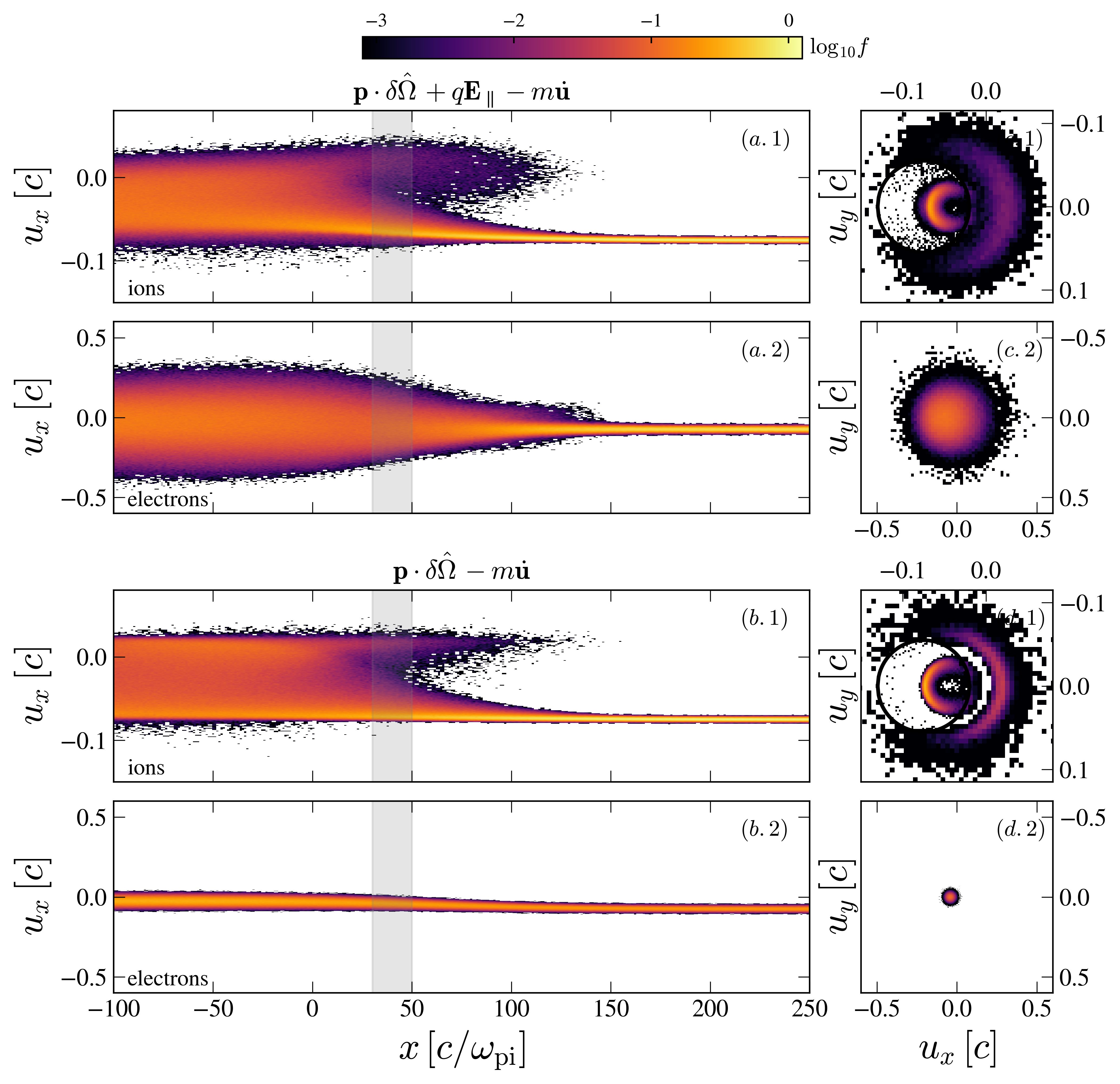
In Fig. 2, we show the phase-space distributions for obtained either from the full MC-P or MC solutions. Essentially, the second case reduces to the contribution of the purely motional electric field. In this case, electrons heat up almost adiabatically, trapped and compressed by the turbulence, ending with a negligible downstream temperature: . When the full solution is considered, we observe that electrons are predominantly heated by the longitudinal electrostatic field, giving rise to a downstream temperature ratio , consistent with the full PIC simulations. We note that the transport equation assumes small pitch-angle scattering for particles in microturbulence, which is valid for ions but not necessarily for electrons due to their smaller Larmor radius. We have checked that accounting for correlated scattering for electron transport does not significantly affect the dynamics [31].
The transport equation (I) captures the essential electron dynamics. With the general goal of building a reduced model for the shock profile and electron heating, we now derive the set of fluid equations for the electron distribution. We note that the following equations and the previously introduced Fokker-Planck description are not supposed to be valid for ion species for which the diffusive approximation would fail across the shock transition. However, a closed form of the fluid equation for the electrons can be derived in the diffusive approximation from the first moments of the distribution. We decompose the total stress-energy tensor in terms of thermal pressure and number current components. In the thermal part of the distribution, we assume that the scattering frequency is independent of the particle momentum [44]. A more complex polynomial dependence of would be relevant to electron injection and acceleration, which is left for future work. Neglecting anomalous heat transport , relevant to the high-energy component of the distribution, we obtain a solution for the conserved current across the shock transition . Moments of Eq. (I) then give:
| (5) |
where is the ram pressure at . With an explicit form for the dominant non-adiabatic heating rate of the electrons in terms of the amplitude of the coherent electrostatic field, we now derive a closed form for the electron-ion coupling.
The dynamics of electrons, trapped in the turbulence, is well characterized by the diffusive approximation. We distinguish two extreme regimes for the ions: diffusive () and unscattered regimes (). Unscattered ions are only subject to the electric field deceleration and fully isotropize in the downstream. As verified in PIC simulations, quasi-neutrality between the reflected beam charge density and background contribution is observed in the full shock precursor. Given a charge density profile for the reflected beam and background ion velocity , we obtain [31]. The electric field then only results from the relative drift between electrons and ions if .
Assuming a weak deceleration of ions across the shock transition size and neglecting the beam contribution, the system is fully parametrized by a single parameter that represents the number of electron scattering events across the shock transition times the electron-to-ion mass ratio. In the absence of another relevant scale, should be solely determined by the structure of the turbulent field. In such conditions, the scattering frequency of the ions determines the typical shock transition size . Therefore, corresponds to the typical ratio between the electron and ion scattering frequencies, i.e., .
For a linear deceleration profile of in , we obtain [31]. One can then derive the heating rate to the leading order in :
| (9) |
giving a fair estimate of the average heating across the shock transition when compared with the full integration.
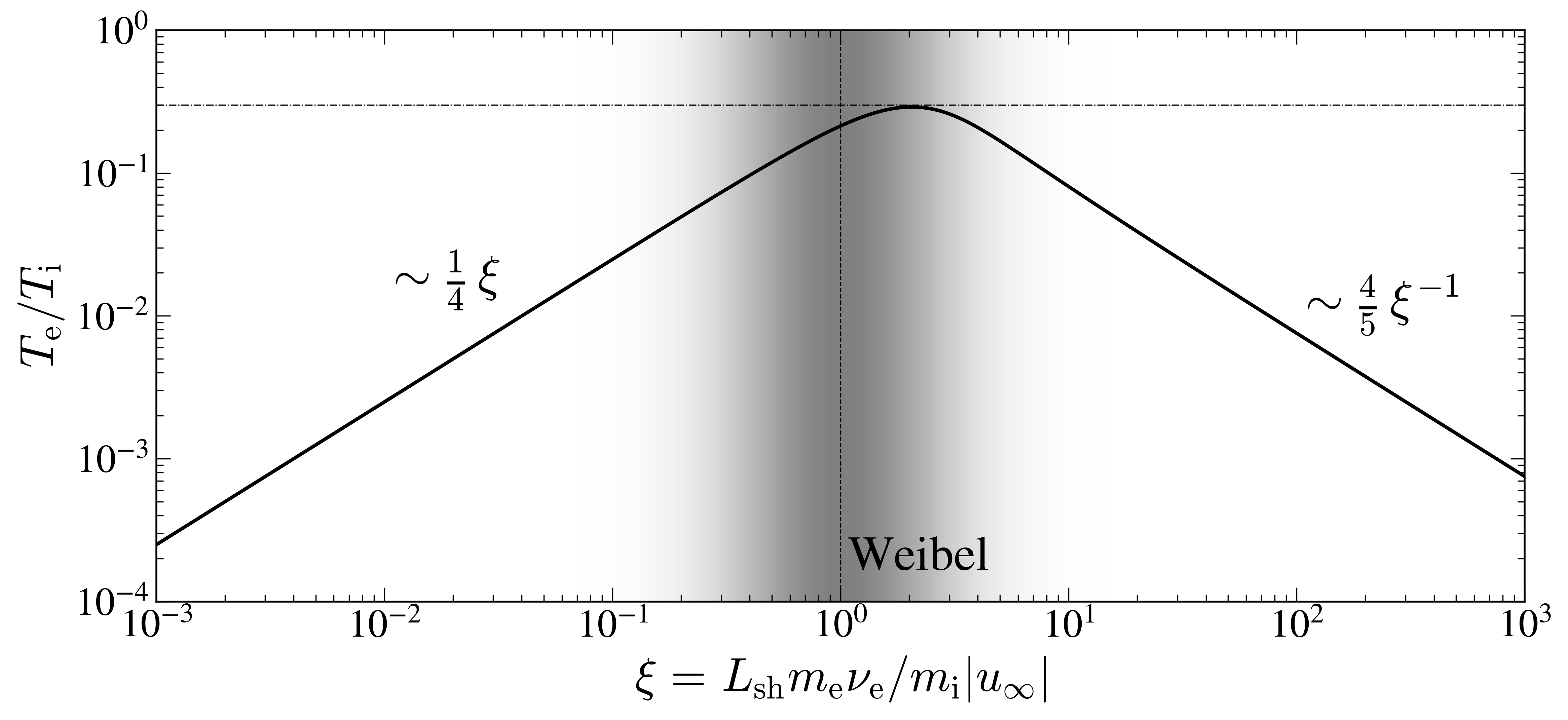
Provided that , the downstream electron pressure is therefore of the order of . The full solution for a linear deceleration, depicted in Fig. 3, confirms that is necessary to recover downstream temperatures on the order of a fraction of unity.
Interestingly, the scaling is also observed in the fully diffusive regime for electrons and ions, suggesting generality of this scaling law. Equations (3) and (4) provide direct estimates of the electron and ion scattering frequencies for the Weibel instability. The ambipolar heating parameter then becomes . Using the values for filament scale in the shock transition, [19, 43, 45], and the field amplitude set by trapping, [46], we obtain , precisely in the range of parameters maximizing the downstream electron temperature in Fig. 3. We note that the model developed here is general in that it could also be applied to other nonlinear processes changing the properties of the magnetic turbulence upstream of the shock, such as non-resonant current-driven instabilities [47], merging [48, 49, 50], cavitation [51], reconnection [52, 53], or kink modes [43]. This would impact primarily through the scale of the turbulent magnetic field – i.e., and . For example, if the field saturates at the scale of the dominant Larmor radius of the beam , untrapped ions result in , and the temperature ratio decreases with . However, if these late nonlinear modes ultimately lead to efficient ion trapping, then we naturally recover , such that the temperature ratio becomes weakly sensitive to subsequent nonlinearities.
In summary, we have developed a self-consistent model for the energy partition in high Mach number collisionless blast waves. The heating results from the ambipolar electric field that accelerates electrons, which are thermalized by rapid scattering in the Weibel-mediated turbulence. We find that the downstream temperature ratio can be expressed in terms of a single dimensionless parameter determined by the nature of the dominant instability. The heating rate and temperature ratio between electrons and ions exhibit good agreement with ab initio fully kinetic simulations, semi-analytical MC-P solutions, and reduced analytical models. Energy partition peaks around with a weak dependence on higher-order effects in the statistics of electron transport and nonlinear dynamics of the instability. Our model gives a natural interpretation for the thermal partition in shocks particularly relevant to weakly magnetized astrophysical systems and to ongoing laboratory experimental studies. More generally, these findings also open promising avenues for studying electron transport in magnetically dominated systems, for which is set by the coherent Larmor gyroradius, and potential electron injection and acceleration in turbulent shocks.
Acknowledgements.
Acknowledgments — AV acknowledges M. Medvedev, A. Bohdan, S. Okamura, M. Toida, and L. Sironi for insightful discussions. AV acknowledges H. Nagataki and H. Ito at RIKEN and T. Amano and Y. Ohira at the University of Tokyo for their hospitality during the conclusion of this work. AV acknowledges support from the NSF grant AST-1814708 and the NIFS Collaboration Research Program (NIFS22KIST020). FF acknowledges support from the European Research Council (ERC-2021-CoG Grant XPACE No. 101045172). This research was facilitated by the Multimessenger Plasma Physics Center (MPPC), NSF grant PHY-2206607. The presented numerical simulations were conducted on the stellar cluster (Princeton Research Computing). This work was granted access to the HPC resources of TGCC/CCRT under the allocation 2024-AD010415130R1 made by GENCI.References
- Krymskii [1977] G. F. Krymskii, Soviet Physics Doklady 22, 327 (1977).
- Bell [1978a] A. R. Bell, Month. Not. Roy. Astron. Soc. 182, 10.1093/mnras/182.2.147 (1978a).
- Bell [1978b] A. R. Bell, Month. Not. Roy. Astron. Soc. 182, 10.1093/mnras/182.3.443 (1978b).
- Blandford and Ostriker [1978] R. D. Blandford and J. P. Ostriker, Astrophys. J. Lett. 221, L29 (1978).
- Drury [1983] L. O. Drury, Reports on Progress in Physics 46, 973 (1983).
- Blandford and Eichler [1987] R. Blandford and D. Eichler, Phys. Rep. 154, 1 (1987).
- Nikolić et al. [2013] S. Nikolić, G. van de Ven, K. Heng, D. Kupko, B. Husemann, J. C. Raymond, J. P. Hughes, and J. Falcón-Barroso, Science 340, 45 (2013).
- Miceli et al. [2019] M. Miceli, S. Orlando, D. N. Burrows, K. A. Frank, C. Argiroffi, F. Reale, G. Peres, O. Petruk, and F. Bocchino, Nature Astronomy 3, 236 (2019).
- Reynolds et al. [2021] S. P. Reynolds, B. J. Williams, K. J. Borkowski, and K. S. Long, Astrop. J. 917, 55 (2021).
- Ghavamian et al. [2013] P. Ghavamian, S. J. Schwartz, J. Mitchell, A. Masters, and J. M. Laming, Space Science Reviews 178, 633 (2013).
- Raymond et al. [2023] J. C. Raymond, P. Ghavamian, A. Bohdan, D. Ryu, J. Niemiec, L. Sironi, A. Tran, E. Amato, M. Hoshino, M. Pohl, T. Amano, and F. Fiuza, Astrop. J. 949, 50 (2023).
- Reynolds [2008] S. P. Reynolds, Annual Rev. Astron. Astrophys. 46, 89 (2008).
- Feldman et al. [1982] W. C. Feldman, S. J. Bame, S. P. Gary, J. T. Gosling, D. McComas, M. F. Thomsen, G. Paschmann, N. Sckopke, M. M. Hoppe, and C. T. Russell, Phys. Rev. Lett. 49, 199 (1982).
- Johlander et al. [2023] A. Johlander, Y. V. Khotyaintsev, A. P. Dimmock, D. B. Graham, and A. Lalti, Geophys. Res. Lett. 50, e2022GL100400 (2023).
- Huntington et al. [2015] C. M. Huntington, F. Fiuza, J. S. Ross, A. B. Zylstra, R. P. Drake, D. H. Froula, G. Gregori, N. L. Kugland, C. C. Kuranz, M. C. Levy, C. K. Li, J. Meinecke, T. Morita, R. Petrasso, C. Plechaty, B. A. Remington, D. D. Ryutov, Y. Sakawa, A. Spitkovsky, H. Takabe, and H.-S. Park, Nat. Phys. 11, 173 (2015).
- Schaeffer et al. [2017] D. B. Schaeffer, W. Fox, D. Haberberger, G. Fiksel, A. Bhattacharjee, D. H. Barnak, S. X. Hu, and K. Germaschewski, Phys. Rev. Lett. 119, 025001 (2017).
- Fiuza et al. [2020] F. Fiuza, G. F. Swadling, A. Grassi, and et al., Nat. Phys. 10.1038/s41567-020-0919-4 (2020).
- Grassi and Fiuza [2021] A. Grassi and F. Fiuza, Phys. Rev. Res. 3, 023124 (2021).
- Kato and Takabe [2008] T. N. Kato and H. Takabe, Astrophys. J. Lett. 681, L93 (2008).
- Amano and Hoshino [2009] T. Amano and M. Hoshino, Astrop. J. 690, 244 (2009).
- Kato and Takabe [2010] T. N. Kato and H. Takabe, Astroph. J. 721, 828 (2010).
- Kumar et al. [2015] R. Kumar, D. Eichler, and M. Gedalin, Astrophys. J. 806, 165 (2015).
- Guo et al. [2017] X. Guo, L. Sironi, and R. Narayan, Astrop. J. 851, 134 (2017).
- Guo et al. [2018] X. Guo, L. Sironi, and R. Narayan, Astrop. J. 858, 95 (2018).
- Kang et al. [2019] H. Kang, D. Ryu, and J.-H. Ha, Astrop. J. 876, 79 (2019).
- Tran and Sironi [2020] A. Tran and L. Sironi, Astroph. J. Lett. 900, L36 (2020).
- Bohdan et al. [2021] A. Bohdan, M. Pohl, J. Niemiec, P. J. Morris, Y. Matsumoto, T. Amano, M. Hoshino, and A. Sulaiman, Phys. Rev. Lett. 126, 095101 (2021).
- Lezhnin et al. [2021] K. V. Lezhnin, W. Fox, D. B. Schaeffer, A. Spitkovsky, J. Matteucci, A. Bhattacharjee, and K. Germaschewski, Astrop. J. Lett. 908, L52 (2021).
- Morris et al. [2023] P. J. Morris, A. Bohdan, M. S. Weidl, M. Tsirou, K. Fulat, and M. Pohl, Astrop. J. 944, 13 (2023), arXiv:2301.00872 [physics.plasm-ph] .
- Spitkovsky [2005a] A. Spitkovsky, in Astrophysical Sources of High Energy Particles and Radiation, American Institute of Physics Conference Series, Vol. 801, edited by T. Bulik, B. Rudak, and G. Madejski (2005) pp. 345–350.
- [31] Supplementary material .
- Weibel [1959] E. S. Weibel, Phys. Rev. Lett. 2, 83 (1959).
- Fried [1959] B. D. Fried, Phys. Fluids 2, 337 (1959).
- Pelletier et al. [2019] G. Pelletier, L. Gremillet, A. Vanthieghem, and M. Lemoine, Phys. Rev. E 100, 013205 (2019).
- Balescu [1997] R. Balescu, Statistical Dynamics: Matter Out of Equilibrium (Imperial College Press, 1997).
- Lemoine et al. [2019] M. Lemoine, L. Gremillet, G. Pelletier, and A. Vanthieghem, Phys. Rev. Lett. 123, 035101 (2019).
- Vanthieghem et al. [2022a] A. Vanthieghem, M. Lemoine, and L. Gremillet, Astroph. J. Lett. 930, L8 (2022a).
- Plotnikov et al. [2011] I. Plotnikov, G. Pelletier, and M. Lemoine, Astron. Astrophys. 532, A68 (2011).
- Webb [1989] G. M. Webb, Astrophys. J. 340, 1112 (1989).
- Note [1] An analogous form was obtained in [1] for the noninertial contribution uniquely and in [37, 54] in the respective relativistic regimes of collisionless and radiation-mediated blast waves.
- Vanthieghem [2019] A. Vanthieghem, Ph.D. thesis (2019).
- Lemoine [2019] M. Lemoine, Phys. Rev. D 99, 083006 (2019).
- Ruyer and Fiuza [2018] C. Ruyer and F. Fiuza, Phys. Rev. Lett. 120, 245002 (2018).
- Krymskii [1981] G. F. Krymskii, izv. akad. nauk sssr ser. fiz. 45, 461 (1981).
- Swadling et al. [2020] G. F. Swadling, C. Bruulsema, F. Fiuza, D. P. Higginson, C. M. Huntington, H.-S. Park, B. B. Pollock, W. Rozmus, H. G. Rinderknecht, J. Katz, A. Birkel, and J. S. Ross, Phys. Rev. Lett. 124, 215001 (2020).
- Davidson et al. [1972] R. C. Davidson, D. A. Hammer, I. Haber, and C. E. Wagner, Phys. Fluids 15, 317 (1972).
- Bell [2004] A. R. Bell, Month. Not. Roy. Astron. Soc. 353, 550 (2004).
- Medvedev et al. [2005] M. V. Medvedev, M. Fiore, R. A. Fonseca, L. O. Silva, and W. B. Mori, Astrop. J. Lett. 618, L75 (2005).
- Vanthieghem et al. [2018] A. Vanthieghem, M. Lemoine, and L. Gremillet, Phys. Plasmas 25, 072115 (2018).
- Zhou et al. [2020] M. Zhou, N. F. Loureiro, and D. A. Uzdensky, J. Plasma. Phys. 86, 535860401 (2020).
- Peterson et al. [2021] J. R. Peterson, S. Glenzer, and F. Fiuza, Phys. Rev. Lett. 126, 215101 (2021).
- Matsumoto et al. [2017] Y. Matsumoto, T. Amano, T. N. Kato, and M. Hoshino, Phys. Rev. Lett. 119, 105101 (2017).
- Bohdan et al. [2020] A. Bohdan, M. Pohl, J. Niemiec, S. Vafin, Y. Matsumoto, T. Amano, and M. Hoshino, Astrop. J. 893, 6 (2020).
- Vanthieghem et al. [2022b] A. Vanthieghem, J. F. Mahlmann, A. Levinson, A. Philippov, E. Nakar, and F. Fiuza, Month. Not. Roy. Astron. Soc. 511, 3034 (2022b).
- Risken [1989] H. Risken, The Fokker-Planck equation. Methods of solution and applications (1989).
- Deligny [2021] O. Deligny, Astrophys. J. 920, 87 (2021).
- Spitkovsky [2005b] A. Spitkovsky, in Astrophysical Sources of High Energy Particles and Radiation, American Institute of Physics Conference Series, Vol. 801, edited by T. Bulik, B. Rudak, and G. Madejski (2005) pp. 345–350.
— Supplementary Information —
I Transport in the diffusive limit
We detail the electron semi-dynamical equation and closure for electrons in the diffusive limit. The interaction with the Weibel microturbulence first reduces to a pure pitch angle scattering in the scattering center frame . The equation of motion for a single particle reads:
| (10) |
where is the drift velocity of the in the shock front frame and is a stochastic process. The stochastic variable is a linear combination of the generators of the Lie algebra of the rotation group corresponding to pitch-angle scattering in the turbulent magnetic field [38]. In other words, the infinitesimal scattering operator is decomposed on the generators of the Lie algebra:
| (11) | ||||
| (12) |
We can now compute the diffusion coefficient of the transport equation deriving from the above Langevin equations in the respective dimensions. Note that drift and diffusion coefficients are uniquely determined from the Langevin equation. To do so, it is convenient to perform a change in variables where is the pitch-angle cosine. The SDE for momentum then reduces to
| (13) |
and the random part of the pitch-angle variation respectively reduces to
| (14) | |||
| (15) |
such that, for isotropic pitch-angle scattering, the diffusion coefficients reduce to and [55]. The auto-correlation function
| (16) |
depends on the nature of the stochastic process. In the standard case of a Gaussian white noise, the correlation function reduces to
| (17) |
where is the pitch-angle scattering frequency. The differential equation (10) is equivalent to the following transport equation in the shock-front frame where the system is assumed stationary:
| (18) |
where the right-hand side is the operator for elastic scattering in in 3D with the pitch-angle cosine. For a two-dimensional distribution, the operator reduces to . In the diffusive limit, the distribution function is expanded in Legendre polynomials . The transport of electrons is then modeled as a Fokker-Planck process. The above equation, projected along the first Lagrange polynomial, gives:
| (19) | |||
| (20) |
Neglecting terms in gives the following approximations for :
| (21) |
which can be inserted in (19) to obtain a Fokker-Planck equation. We only consider the leading terms of the equation, assuming that the contribution from the electric field is dominant. The right-hand side components correspond to diffusive heating in the coherent electrostatic field, spatial diffusion, and cross-momentum-space diffusion. Core heating of the electrons is mainly affected by the first term, while the second and third components affect the high-energy part of the distribution.
II Scattering and correlation
Integration of the Langevin equation using the MC-P solver demonstrates efficient electron heating through the ambipolar electric field. The main free parameter is the scattering frequency of the particles, estimated analytically in both the trapped and untrapped regimes. To motivate their value, we extract from PIC simulations using two standard estimates and , which implicitly neglects the spatial dependence of the scattering coefficient [35]. The pitch angle is measured, accounting for the phase of the particle as it gyrates inside the turbulence. Measurement of the scattering frequency over tracked particles over time-steps indicates across the shock precursor and continuously increases toward the shock transition through the growth of the magnetic field in scale and amplitude. Consistent with the analytical estimates.
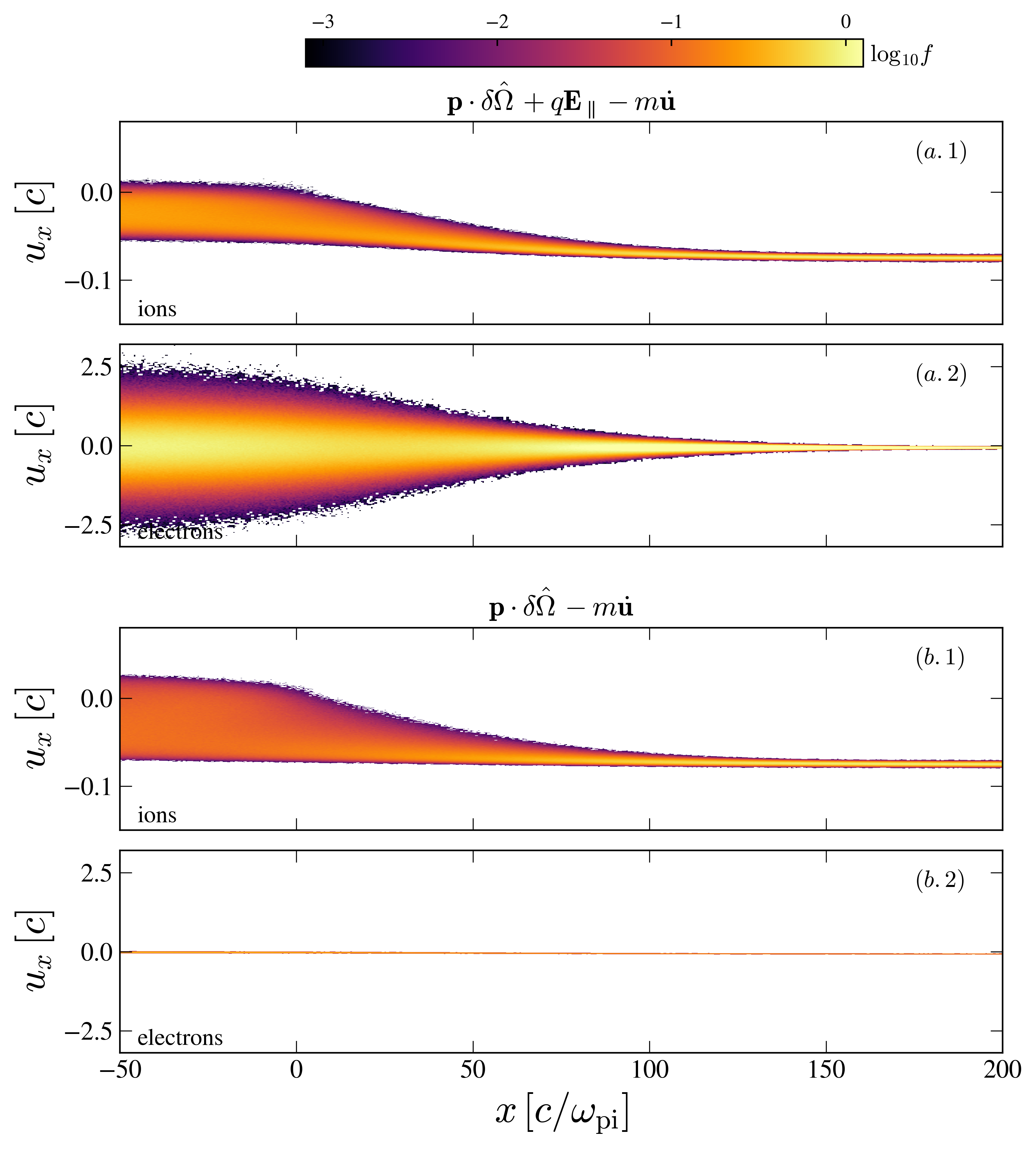
The efficiency of the heating mechanism up to a realistic mass ratio is demonstrated with a solution to the MC-P approach in Fig. 4. We note that the temperature ratio of in the series of MC-P solution is slightly larger than the one obtained from PIC simulations where . While the same electron temperature and dynamics are recovered with , the ions are slightly colder in the MC-P solution such that the temperature ratio is larger.
The white noise limit associated with the transport equation (I) assumes particles undergoing uncorrelated small angle scattering in the microturbulence. This approximation is fair for ions. However, the electron Larmor radius is comparable to or smaller than the typical size of the filaments, and variations in pitch angle are not necessarily independent of time. We now investigate the effect of correlation of the pitch-angle scattering for particles of Larmor radius smaller than the typical scale of the turbulence [56]. In such a case, the auto-correlation function deviates from (17). We hereafter assume the autocorrelation function satisfying:
| (22) |
where is the correlation time of the pitch-angle variation in the microturbulence. The motivation behind the use of colored noise thus becomes more transparent: between scattering events, electrons undergo a series of coherent betatron oscillations and progressively lose coherence as they transition from one structure to another.
To test the effect of correlation, we scatter electrons, assuming an exponentially correlated scattering operator. A colored noise with zero mean and an exponential auto-correlation profile is called a red noise. We obtain the correlated noise from a white noise using the straightforward relation:
| (23) |
We integrate the transport equation with a finite correlation time for the electrons varying between to , see Fig. 5. For , we recover the limit of white noise as expected for correlation time much shorter than the scattering time in the turbulence. The result of the integration is shown in Fig. 5. The profile does not show a significant difference in electron heating over the shock transition. We thus conclude that the standard white noise limit captures the essential mechanism of electron heating.
III Fluid description and downstream temperature
A closed form of the fluid equation can also be derived from the first moments of the distribution. The general form of the moment of order , in the shock front frame, reads:
| (24) |
The current and the longitudinal momentum flux are then, respectively, given by:
| (25) | ||||
| (26) | ||||
| (27) | ||||
| (28) |
from which we obtain the following relations
| (29) | |||
| (30) |
From the moments of the transport equation (I), we obtain the following:
| (31) | |||
| (32) |
To ease comparison, we decompose the longitudinal momentum flux into thermal and ram pressure components such that:
| (33) |
From higher moments of the transport equation and neglecting the contribution of the heat flux, we obtain the following closure relation:
| (34) |
The above Eq. (34) clearly shows the nonadiabatic nature of the turbulent heating in a Joule-like process from diffusion in the coherent electric potential and deceleration of the plasma microturbulence. A closed form of the equation can also be obtained from the kinetic distribution in Eq. (I), assuming to be independent of . The first moment of Eq. (I) readily gives:
| (35) |
Inserting this closure into Eq. (31) to leading order in , we obtain:
| (36) |
Neglecting in Eq. (36), we directly have a solution for . From quasi-neutrality , we then obtain an estimate of the ambipolar field in terms of the Weibel frame velocity, the ion velocity, and the charge density of the beam of reflected ions . The rest of the calculations leading to Eq. (5) in the letter are outlined in the main text. Using the relations we derived, we now discuss the direct estimate of the electric field across the shock transition. We consider a linear deceleration region between of the form:
| (37) |
With a linear deceleration profile and neglecting ion scattering and beam contribution across the shock transition, electron pressure is directly obtained from the following set of equations:
| (38) | |||
| (39) |
The numerical solution, shown in the main paper, peaks at for , in good agreement with particle-in-cell simulations.
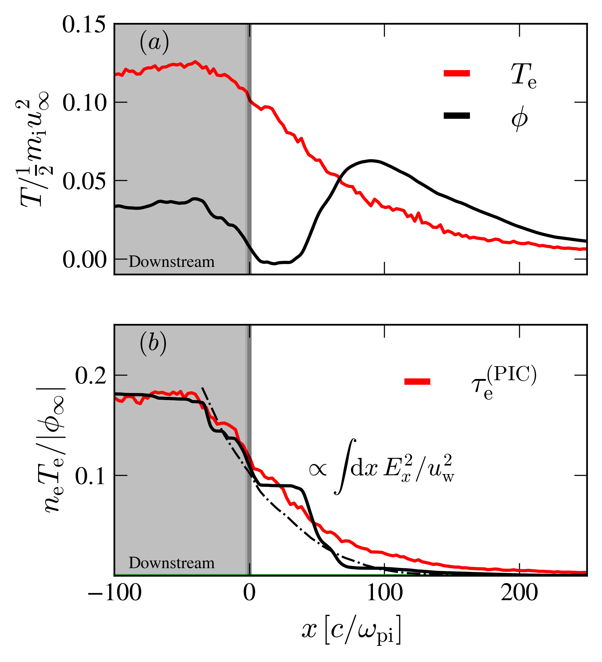
The diffusion coefficient, proportional to , leads to a heating rate independent of the sign of the electric field. This is observed in Fig. 6.a, where the change of sign in , corresponding to the modulation of , is attributed to the influence of the beam captured in the full expression . In a region where , the sign of the electric field will experience a reversal, as observed in the simulation. However, adiabatic cooling is negligible due to the diffusive nature of the heating. To illustrate this, a comparison between the predicted and measured electron pressure is shown in the bottom panel Fig. 6. The predicted pressure is multiplied by an arbitrary factor of order unity accounting for corrections to the dimensionality of the scattering operator and amplitude of the scattering frequency. The profile of the electrostatic potential obtained from the PIC simulation is shown in the top panel. Our reduced analytical model neglects the contribution of the beam in the total heating rate. To validate this hypothesis, Fig. 6.b shows the associated analytical temperature profile obtained by direct integration of Eqs. (38)-(39). The ion and Weibel velocity profiles were extracted directly from the PIC simulation to close the system. The analytical profile captures the trend and amplitude of energy partition between species.
IV Convergence
To support the analytical and semi-analytical models described in the letter, we performed a series of 2D3V simulations with the massively parallel kinetic code Tristan-MP [57]. Here, we describe the series of tests ensuring convergence of the electron temperature in the shock downstream. With run A, the main simulation, and a constant , we vary the numerical resolution within in run B, increased the shock velocity from to in run B, and increased the phase-space resolution in run C. We found a good convergence of the electron temperature.
| Run | ||||||
|---|---|---|---|---|---|---|
| A | ||||||
| B | ||||||
| C | ||||||
| D |