One-Class Classification as GLRT for
Jamming Detection in Private 5G Networks

Abstract

Fifth-generation (5G) mobile networks are vulnerable to jamming attacks that may jeopardize valuable applications such as industry automation. In this paper, we propose to analyze radio signals with a dedicated device to detect jamming attacks. We pursue a learning approach, with the detector being a convolutional neural network (CNN) implementing a generalized likelihood ratio test (GLRT). To this end, the CNN is trained as a two-class classifier using two datasets: one of real legitimate signals and another generated artificially so that the resulting classifier implements the GLRT. The artificial dataset is generated mimicking different types of jamming signals. We evaluate the performance of this detector using experimental data obtained from a private 5G network and several jamming signals, showing the technique’s effectiveness in detecting the attacks.

I Introduction

Fifth-generation (5G) networks have become increasingly important in everyday life scenarios over recent years, because of their technical advances in wireless communications[1]. Since they also support mission-critical applications such as smart manufacturing or autonomous driving, they should be adequately protected against security attacks.

Nowadays, wireless intrusion prevention systems (WIPS) monitor the security status of the transmission channel from the link layer up, aggregating measurements from the different communication layers[2][3]. Several attackers, however, have learned to hide their malicious behaviors at layer 2 and above. Thus, a recent trend is to exploit the physical layer to provide security services, often relying on machine learning [4]. This paper leverages the recent work [5] that introduced deep learning (DL) to detect jamming attacks. Any device that injects noise into the band used for communication is considered a jammer aiming at making the service unavailable to cellular devices. In this context, jamming and anti-jamming strategies have been recently surveyed in [6].

We consider the WIPS as a one-class classification problem, also called anomaly detection. Note that the classifier also needs to detect jamming signals that have never been seen before, and on which it may not have been trained. Indeed, assuming a specific attack pattern may even lead to vulnerabilities in the learned detection model that an informed attacker may exploit. However, this constraint makes the design of anti-jamming techniques more challenging. A typical solution of such a one-class classification problem is the generalized likelihood ratio test (GLRT), which is used in various contexts, e.g., [7, 8]. Still, this solution requires the knowledge of the statistics of received signals in legitimate conditions, which may be problematic to obtain, due to the different characteristics of the radio propagation environments where the private networks are deployed.

In this paper, we frame the WIPS as a one-class classification problem and tackle it by a GLRT implemented via supervised learning, in particular a convolutional neural network (CNN). As proven in [9], under suitable hypotheses, a DL model trained with supervised learning can indeed learn the GLRT, and thus can be used for one-class classification. Thus, drawing inspiration from [9], the detector builds an artificial dataset for the jammer with uniform distribution in the in-phase quadrature (IQ) sample domain and uses it during the training phase of the DL model. The accuracy of the trained model is evaluated using samples taken from a real-world jammer, thus modeling the discrepancy between the detector’s prior knowledge and the actual attack statistics. The trained model performance is compared to the solution of [5] that uses convolutional autoencoder (CAE), a DL model that implements a full one-class classification problem. The comparison is based on experimental data, where the detector, jammer, and 5G base station are implemented as software-defined radios (SDRs).

After this introduction, Section II describes the studied system and assumptions. Section III explains the dataset generation. Section IV details the models’ design for jamming detection. Section V shows the obtained results. Finally, we draw the main conclusions in Section VI.

II System Model

II-A Security Scenario

We consider the security scenario depicted in Fig. 1 representing a typical private 5G network used in industrial applications. We assume that there is at least one wireless channel for communication available, provided by the 5G base station, called gNodeB (gNB). The wireless channel is used by the user equipment (UE) to transmit data whenever necessary. The availability of the communication is threatened by the jammer, which transmits artificial noise in the band allocated for the transmission of data. This band is monitored by the watchdog, which permanently records the wireless signal in the form of IQ samples. Given this stream of IQ samples, the watchdog aims to detect the attack through a pre-trained machine-learning model.

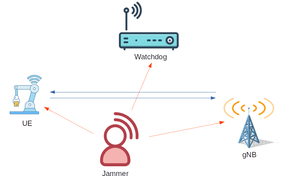
Figure 1: Considered security scenario: blue arrows indicate legitimate cellular communications and red arrows indicate the jamming signals.

Adopting the concept of loose observation[5] we assume that the watchdog knows a priori the basic radio parameters of communication, i.e., carrier frequency $f_{\rm c}$, bandwidth $W$, and pilot structure.

II-B Detector Design via Machine Learning

In this Section we recall the results of [9], detailing how to derive a one-class classifier via machine learning having the same performance as the GLRT.

First, we formalize the one-class classification problem. We aim to design a detector to distinguish between a received signal without jamming and one affected by a jamming attack. We consider a scenario where we do not have a database of attack signals, thus the training should be done without prior knowledge of the attack signal.

Formally, let $\mathcal{H}_{0}$ be the hypothesis class of no-jamming and $\mathcal{H}_{1}$ the hypothesis class of jamming, the jammer detection on a security metric $\Gamma$, which in turn is a function of the input $\bm{X}$ to be tested, is performed as

$$\hat{\mathcal{H}}=\begin{cases}\mathcal{H}_{0}&\mbox{if }\Gamma(\bm{X})<\tau,\\ \mathcal{H}_{1}&\mbox{if }\Gamma(\bm{X})\geq\tau,\\ \end{cases}$$ (1)

where $\tau$ is the chosen threshold. Thus, we can measure accuracy as the probability of false alarm (FA) and misdetection (MD) defined as

$$P_{\rm FA}={\mathbb{P}}[\hat{\mathcal{H}}=\mathcal{H}_{1}|\mathcal{H}=\mathcal{H}_{0}]\,,$$ (2)

$$P_{\rm MD}={\mathbb{P}}[\hat{\mathcal{H}}=\mathcal{H}_{0}|\mathcal{H}=\mathcal{H}_{1}]\,.$$ (3)

A well-known result is that, for a fixed FA, the minimum MD is achieved by using the likelihood ratio

$$\Gamma_{\rm LR}(\bm{X})=\frac{p(\bm{X}|\bm{X}\in\mathcal{H}_{0})}{p(\bm{X}|\bm{X}\in\mathcal{H}_{1})}.$$ (4)

However, such a test requires the knowledge of input statistics when under attack which is not provided in a security scenario, as it would require the cooperation of the attacker during training. Thus, the solution in the statistical framework is resorting to the GLRT,

$$\Gamma_{\rm GLRT}(\bm{X})={p(\bm{X}|\bm{X}\in\mathcal{H}_{0})}\,.$$ (5)

Such a solution is often used in security applications and is provably optimal in some contexts [10]. This solution belongs to the statistical domain, where a legitimate dataset distribution is given.

In this work instead, we assume that we only have the dataset $\mathcal{D}_{0}$ of received signals $\bm{X}$ when operating without jamming. Thus, we have $\mathcal{D}_{0}\sim p(\bm{X}|\bm{X}\in\mathcal{H}_{0})$.

We tackle the one-class classification problem by combining a two-class classifier with an artificial dataset $\mathcal{D}^{\star}_{1}$, generated to be uniform over the input domain. The two-class classifier is then implemented as a CNN, trained with dataset $\mathcal{D}=\{\mathcal{D}_{0},\mathcal{D}^{\star}_{1}\}$. The following Theorem [9][Th. 1] states that such a classifier has the same performance as the GLRT based classifier, i.e., (5) paired with (1).

Theorem 1.

[9][Th. 1] A neural network (NN) trained with a mean squared error (MSE) loss function over the two class dataset $\mathcal{D}=\{\mathcal{D}_{0},\mathcal{D}^{\star}_{1}\}$, obtain one-class classifiers equivalent to the GLRT, when a) the training converges to the configuration minimizing the loss functions of the two models, and b) the NN is complex enough or the dataset $\mathcal{D}_{0}$ is large enough, the training converges to the configuration minimizing the loss functions of the two models.

III Data Collection and Augmentation

In this section, we will detail how we collected the no-jamming dataset $\mathcal{D}_{0}$, the jamming dataset $\mathcal{D}_{1}$ (not used for training, but to assess the performance in testing), and the artificial dataset $\mathcal{D}_{1}^{\star}$ (used for training). We recall that to emulate the one class-classification context, only $\mathcal{D}_{0}$ and $\mathcal{D}_{1}^{\star}$ have been used for training the detector, while the testing phase is performed between $\mathcal{D}_{0}$ and $\mathcal{D}_{1}$.

III-A Laboratory Setup

In the laboratory setup, the devices described above were implemented as SDRs, specifically:

• The gNB is implemented based on srsRAN 23.5 [11] and the bladeRF 2.0 micro xA4 SDR-frontend[12]. It generates a 5G NR signal with bandwidth $W=$20\text{\,}\mathrm{MHz}$$ in the n78 band at center frequency $f_{\rm c}=$3.75\text{\,}\mathrm{GHz}$$ in time division duplexing (TDD) mode.

• The watchdog and the jammer are implemented based on GNURadio and the ADALM-PLUTO SDR-frontend [13] and operate at $40$ MHz bandwidth.

• The UE is an unmodified 5G smartphone, namely the Samsung Galaxy A90 (model version: SM-A908B).

The core network is provided by Open5GS 2.6.4 [14].

III-B Dataset Creation

Using full bandwidth, the jammer permanently transmits complex noise (uniform and Gaussian), as specified below, while the watchdog permanently records IQ samples. After having recorded a certain number of IQ samples, the watchdog creates IQ bitmaps in a resolution of $128\times 128$ fixing the I and Q axis interval to $[-1.5;1.5]$. Two relevant examples for these bitmaps are given in Fig. 2

The recorded IQ data contains the following cases:

1. Empty channel: gNB actively transmitting beacons but UE not transmitting, while the jammer is not active.

2. Transmitting channel: UE and/or gNB are transmitting data in TDD mode, while the jammer is not active.

3. Jammer ON: UE and gNB occasionally send signals (e.g., beacons, connection requests) but no communication is possible.

4. Artificial attack data: according to the GLRT two kinds of synthetic IQ plots are created: the first one is a uniform distribution of samples over two dimensions (2D), while the second one is a uniform distribution of samples over a frame, as depicted in Fig. 3.

IQ bitmaps from the first two cases are classified as legitimate and collected in $\mathcal{D}_{0}$. Bitmaps from case Jammer ON are considered to be in $\mathcal{D}_{1}$. IQ bitmaps from the last case are placed in the artificial dataset $\mathcal{D}_{1}^{\star}$.

The number of IQ samples per bitmap $n$ corresponds to the time window covered per bitmap. This parameter was studied for the levels $n=\{256,1024,2048\}$. To save space, we will only present results for $n=256$ in this paper but will comment on the other levels.

(a) IQ bitmap with no transmission ongoing with time window equal to 1024 samples.

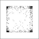
(b) IQ bitmap with transmission ongoing with time window equal to 1024 samples with an unequalized 4-QAM.

Figure 2: Example of two IQ bitmaps.

(a) IQ bitmap of a uniform distribution of samples over the 2D space with time window equal to 1024 samples.

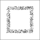
(b) IQ bitmap of a uniform distribution over a frame with time window equal to 1024 samples.

Figure 3: Two types of virtual dataset for training the DL models.

IV Jamming Detection Models

We adopt two machine learning methods and use them for a systematic comparison as follows: Models built with CAE will serve as our baseline, since this method only uses data from the not-jammed scenarios, i.e., $\mathcal{D}_{0}$. CNN, instead, will make additional use of the artificial dataset $\mathcal{D}_{1}^{\star}$ and, therefore, may or may not outperform the baseline. Let us now describe both methods in detail.

IV-A Convolutional Neural Network (CNN)

Our proposed solution includes a CNN, which is a DL model trained with the no-jamming $\mathcal{D}_{0}$ and the artificial samples $\mathcal{D}_{1}^{\star}$. As discussed in Section II, such training methods allow the CNN jamming detector to achieve the performance of the GLRT asymptotically.

The designed model is a CNN, whose structure is given in Table I. The CNN is trained to implement (1), i.e., to return $0$ when $\bm{X}\in\mathcal{D}_{0}$ and $1$ when $\bm{X}\in\mathcal{D}_{1}$ (during training, $\mathcal{D}_{1}^{\star}$). As a loss function, we adopted the binary cross-entropy

$$L=-\frac{1}{N}\sum_{i=1}^{N}y_{i}\cdot\log(\tilde{y}_{i})+(1-y_{i})\cdot\log(1-\tilde{y}_{i}),$$ (6)

where $\tilde{y}_{i}$ is the output for the $i$-th input sample.

TABLE I: Structure of the Employed CNN

	Layer	Output size	No. of parameters
	Input	$128\times 128\times 1$	$0$
	Convolutional 1	$64\times 64\times 64$	$640$
	Average Pooling	$32\times 32\times 64$	$0$
	Convolutional 2	$16\times 16\times 32$	$18464$
	Flatten	$8192$	$0$
	Dense	$32$	$262176$
	Dense	$1$	$33$

IV-B Convolutional Autoencoder (CAE)

As our baseline, we use the solution of [5]. This solution is based on an CAE, often used for one-class classification [15]. An autoencoder (AE) is a DL structure that, given an input $\bm{X}$, compresses it to a latent space with reduced dimensionality (Encoder) and then reconstructs (Decoder) from such compressed representation the original input, outputting $\bm{Y}$. A CAE is an AE that exploits spatial correlation of the 2D data structure by using convolutional filters.

During training, the goal of the model (whose structure is given in Table II) is then to minimize the reconstruction error, defined by the MSE loss function

$$\bar{\Lambda}={\mathbb{E}}[\Gamma],\quad\Lambda(\bm{X})=||\bm{X}-\bm{Y}||^{2}.$$ (7)

When trained only in the no-jamming dataset, $\mathcal{D}_{0}$, during testing the MSE is expected to be small only when $\bm{X}\in\mathcal{D}_{0}$, while, vice-versa, the model should output higher MSEs on the jamming cases, $\bm{X}\in\mathcal{D}_{1}$. The security metric to be used for jamming detection is then $\Gamma_{CAE}(\bm{X})=\Lambda(\bm{X})$.

TABLE II: Structure of the Employed CAE

	Layer	Output size	No. of parameters
Encoder	Input	$128\times 128\times 1$	$0$
	Convolutional 1	$64\times 64\times 64$	$640$
	Convolutional 2	$32\times 32\times 32$	$18464$
	Flatten	$32768$	$0$
	Dense	$32$	$1048608$
Decoder	Input	$32$	$0$
	Dense	$32768$	$1081344$
	Reshape	$32\times 32\times 32$	$0$
	Convolutional 1T	$64\times 64\times 32$	$9248$
	Convolutional 2T	$128\times 128\times 64$	$18496$
	Convolutional	$128\times 128\times 1$	$577$

V Numerical Results

This section will detail the training process for CAE and CNN, describe the used performance metrics, and, finally, discuss the numerical results.

V-A Training Process

The training process of the CAE was the same as in [5]. It was performed using $\mathcal{D}_{0}$ (without jamming), based on $4000$ IQ scatter plots. Half of the bitmaps represent empty channels, while the other half represents a busy channel with ongoing transmission. The validation set contains $600$ IQ bitmaps, with the same proportional split between empty and busy channels, whose loss was used to automatize an early stopping with patience set to $4$.

The CNN was trained with $4000$ bitmaps from $\mathcal{D}_{0}$, equally distributed between the two legitimate cases, and $4000$ bitmaps generated with the uniform virtual distribution according to the parameters specified above, collected in the set $\mathcal{D}_{1}^{\star}$. The validation set contains $600$ bitmaps with the same distribution as the training set.

TABLE III: Training and Validations Losses for CAE and CNN

Model	Training	Validation
CAE	$0.0133$	$0.0134$
CNN	$9.7\times 10^{-5}$	$3.8\times 10^{-4}$

The test set was the same for the two models and was composed of $800$ bitmaps: $400$ were taken from legitimate cases, $\mathcal{D}_{0}$, while the other half was taken from three attacking situations, i.e., a jammer that injects uniform or Gaussian noise over all the spectrum or uniform jamming over a frame, all collected in $\mathcal{D}_{1}$.

Table III shows values for the resulting training and validation loss at the end of the training phase for CAE and CNN. As training and validation loss are close, we can conclude that the trained model did not incur overfitting problems.

V-B Performance Metrics

We measure performance in terms of false alarm (FA) and misdetection (MD) rates for a variable threshold of the machine learning output between $0$ to $1$. To simplify comparison, the thresholds providing MD and FA rates of $10^{-2}$ are determined for each model. Then, for each pair of MD-FA curves, the distance between the respective MD and FA thresholds will be measured. The resulting distance value per model can then be compared among the models for a quick overview.

V-C Performance Results

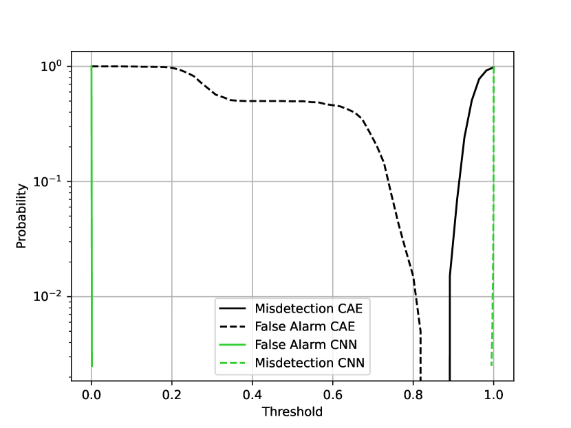
Figure 4: Performance comparison in terms of accuracy between the two models in the case: n$=256$, noise: uniform.

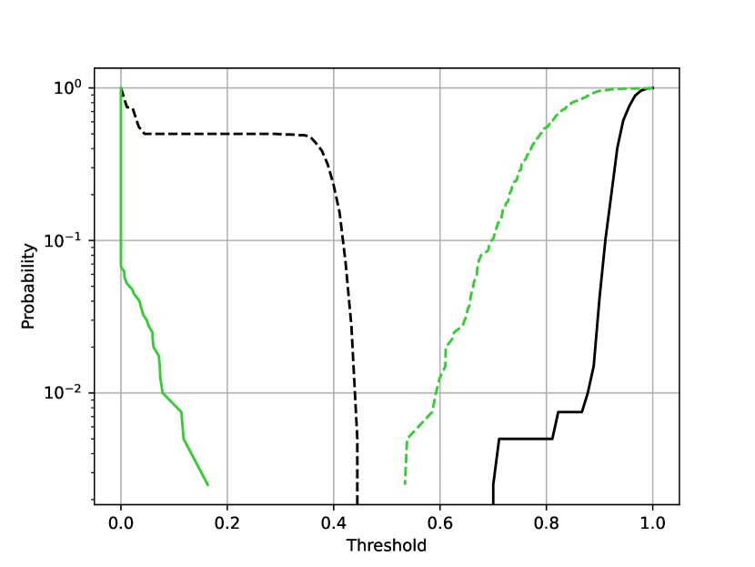
Figure 5: Performance comparison in terms of accuracy between the two models in the case n$=256$, noise: uniform over a frame. Lines and colors are those of Fig. 4.

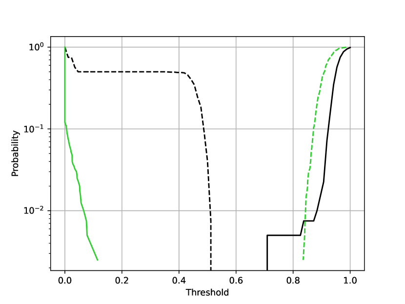
Figure 6: Performance comparison in terms of accuracy between the two models in the case n$=256$, noise: Gaussian. Lines and colors are those of Fig. 4.

Fig. 4, 5, and 6 compare FA and MD rates achieved with both models for the three different jamming cases.

With uniform noise, the CNN clearly shows a better performance than the CAE.

With frame-like noise (see Fig. 3b) the CNN still outperforms CAE. This is indicated by the separation between the FA and MD curves for the CNN, which is $0.5$ substantially wider than the separation of $0.35$ with CAE. This is a performance gain of $43\%$ over the baseline.

With Gaussian noise, the CNN model reaches an even higher performance gain. CAE produces a separation between the two curves of approximately $0.35$, while the CNN produces a separation of approximately $0.75$. Thus, the CNN with artificial data outperforms the baseline by $114\%$.

In addition to $n=256$ IQ samples per bitmap, models created and tested with larger time windows were also studied. With a window size of $n=1024$ samples, the separation of the curves improves, compared to CAE, but the gain is smaller than with $n=256$. A time window of $2048$ samples, on the other hand, significantly improved separation and gain for the case of uniform noise.

VI Conclusions

For the relevant use case of private 5G networks, we proposed a method to improve the accuracy of a jamming detector at the physical layer.

To keep the detection model independent of the attacker but still profit from supervised learning, we included synthetically generated attack data. The resulting accuracy gains demonstrate improved threat detection compared to the unsupervised learning approach used in previous works.

In light of the promising results and the sensitivity of the subject matter, further studies on the subject will follow.

References

- [1] Ericsson, “5G driving revenue growth in top 20 markets,” Ericsson Mobility Report — Business Review edition, Feb. 2023.
- [2] S. Hong, K. Kim, and S.-H. Lee, “A hybrid jamming detection algorithm for wireless communications: Simultaneous classification of known attacks and detection of unknown attacks,” IEEE Communications Letters, vol. 27, no. 7, pp. 1769–1773, 2023.
- [3] B. Chatfield, R. J. Haddad, and L. Chen, “Low-computational complexity intrusion detection system for jamming attacks in smart grids,” in Proc. of the International Conference on Computing, Networking and Communications (ICNC), 2018, pp. 367–371.
- [4] T. M. Hoang, A. Vahid, H. D. Tuan, and L. Hanzo, “Physical layer authentication and security design in the machine learning era,” IEEE Communications Surveys & Tutorials, pp. 1–1, Feb. 2024.
- [5] M. Varotto, S. Valentin, and S. Tomasin, “Detecting 5G signal jammers with autoencoders based on loose observations,” in Proc. of IEEE Globecom Workshops (GC Wkshps), 2023, pp. 160–165.
- [6] H. Pirayesh and H. Zeng, “Jamming attacks and anti-jamming strategies in wireless networks: A comprehensive survey,” IEEE Communications Surveys & Tutorials, vol. 24, no. 2, pp. 767–809, Mar. 2022.
- [7] F. Ardizzon, P. Casari, and S. Tomasin, “A RNN-based approach to physical layer authentication in underwater acoustic networks with mobile devices,” Computer Networks, vol. 243, p. 110311, Mar. 2024, URL verified on 2024-04-15. [Online]. Available: https://www.sciencedirect.com/science/article/pii/S1389128624001439
- [8] L. Crosara, F. Ardizzon, S. Tomasin, and N. Laurenti, “Worst-case spoofing attack and robust countermeasure in satellite navigation systems,” IEEE Transactions on Information Forensics and Security, vol. 19, pp. 2039–2050, Dec. 2023.
- [9] F. Ardizzon and S. Tomasin, “Learning the likelihood test with one-class classifiers,” 2024, arXiv, URL verified on 2024-04-15. [Online]. Available: https://arxiv.org/abs/2210.12494
- [10] O. Zeitouni, J. Ziv, and N. Merhav, “When is the generalized likelihood ratio test optimal?” IEEE Transaction on Information Theory, vol. 38, no. 5, pp. 1597–1602, Sept. 1992.
- [11] Software Radio Systems, “srsRAN project documentation,” online, Jun. 2023, URL verified on 2024-04-15. [Online]. Available: https://docs.srsran.com/projects/project/en/latest/
- [12] Nuand LLC, “Datasheet bladeRF 2.0 micro,” online, 2023, URL verified on 2024-04-15. [Online]. Available: https://www.nuand.com/bladerf-2-0-micro/
- [13] R. Getz, “ADALM-PLUTO detailed specifications,” online, Feb. 2021, URL verified on 2024-04-15. [Online]. Available: https://wiki.analog.com/university/tools/pluto/devs/specs
- [14] S. Lee, “Open5GS: documentation,” online, Jul. 2023, URL verified on 2024-04-15. [Online]. Available: https://open5gs.org/open5gs/docs/
- [15] Z. Chen, C. K. Yeo, B. S. Lee, and C. T. Lau, “Autoencoder-based network anomaly detection,” in Proc. of Wireless Telecommunications Symposium (WTS), 2018, pp. 1–5.