Detecting 5G Narrowband Jammers with CNN, $k$-nearest Neighbors, and Support Vector Machines

Abstract

5G cellular networks are particularly vulnerable against narrowband jammers that target specific control subchannels in the radio signal. One mitigation approach is to detect such jamming attacks with an online observation system, based on machine learning. We propose to detect jamming at the physical layer with a pre-trained machine learning model that performs binary classification. Based on data from an experimental 5G network, we study the performance of different classification models. A convolutional neural network will be compared to support vector machines and $k$-nearest neighbors, where the last two methods are combined with principal component analysis. The obtained results show substantial differences in terms of classification accuracy and computation time.

I Introduction

5G cellular networks promise improved latency, data rate, and the support of mission critical applications. Consequently, their application in automotive and smart manufacturing is rapidly increasing [1].

Unfortunately, 5G radio signals are particularly vulnerable to jamming attacks [2]. A jammer performs a denial of service attack by emitting interference in the frequency band used by, e.g., a 5G network. By targeting specific control subchannels in the signal, it is sufficient to interfere only with a small fraction of the overall bandwidth to disrupt the service. Such narrowband jammer can be easily implemented as an software defined radio (SDR) at low cost. One very effective narrowband jamming approach [3] targets the signal synchronization block (SSB) in the 5G signal, which is critical to establish and to maintain 5G communication. Other narrowband jamming approaches are discussed in [2].

One mitigation approach is to detect jamming attacks by an online wireless intrusion prevention systems (WIPS). Such detection often relies on specific parameters such as signal-to-noise-ratio (SNR), bit error rate (BER), packet error rate (PER) [4], or on measurements aggregated over multiple network layers [5]. Such high-level measurements, however, may be easily evaded by a jammer. For instance, a short jamming impulse in the SSB-subband effectively disrupts 5G communication [3] but barely affects the, usually time-averaged, SNR of the mainband. The same argument holds for SNR derivatives such as BER and PER. Detection based on measuring the quality of the radio signal at the physical layer [6], requires accurate synchronization in time and frequency. This not only leads to costly implementation but may also mislead the classification due to normal clock differences in a cellular network.

In this paper, we propose a WIPS to detect 5G narrowband jammers. This detection is based on spectrograms of the 5G radio signal and a pre-trained machine learning model for binary classification. These spectrograms are obtained from an experimental 5G network, which is occasionally attacked by an SSB jammer. The objective of our paper is to compare how accurate and how quickly the SSB jammer can be detected with different machine learning models. To this end, we compare classification accuracy and computational complexity of a convolutional neural network (CNN) with support vector machines (SVMs) and $k$-nearest neighbors (KNNs). SVM and KNN are combined with principal component analysis (PCA) for dimensionality reduction.

The considered security scenario is a typical private 5G network used in industrial applications. We assume at least one available wireless channel for communication, provided by a 5G base station, called gNB. The channel is utilized by the User Equipment (UE) to transmit or receive data whenever need be. The communication channel may be attacked by a jammer in close range of the gNB.

This network is monitored by a watchdog – a separate network element placed within range of the gNB. The watchdog receives radio signals and converts them to the digital baseband in the form of in-phase and quadrature (IQ) samples. Based on these IQ samples, anomaly detection is performed based on a pre-trained machine learning model.

This configuration has several benefits. The watchdog can be deployed independently of the cellular network and, as a mere receiver, does not transmit signals that can be detected. Thus, it can be deployed invisible to a potential attacker. The watchdog is simpler and easier to construct than a communication device, since it can still operate effectively with imperfect synchronization in time and frequency.

The following Sec. II covers the creation of the dataset while in Sec. III the machine learning models are explained. In Sec. IV results are discussed and Sec. V concludes the paper.

II Dataset Description

We assume that the watchdog knows the basic radio parameters such as center frequency $f_{c}$, bandwidth $W$, and the pilot structure. This assumption is feasible, as these parameters are constant and known to the operator of the radio access network (RAN). Based on these parameters, the detector receives radio signals, computes a stream of IQ samples and spectrograms. This signal processing and the dataset creation are briefly explained in Sec. II-B.

The collected spectrogram data is labeled in three cases:

1. Empty channel, not jammed: the jammer is not active; gNB periodically transmits beacons but UE is not transmitting

2. Ongoing transmission, not jammed: the jammer is not active; UE and/or gNB are transmitting and receiving data in TDD mode

3. Jammed: the jammer is injecting uniform noise into the SSB subchannel; UE and gNB occasionally transmit signals (e.g., beacons, connection requests) but cannot decode received signals

The first two cases are classified as legitimate and labelled with $0$, while the third case is classified as an attack and labelled with $1$.

II-A Experimental Setup

Fig. 1 shows the experimental setup. We are running a private 5G network in the n78 frequency band with center frequency $f_{c}=3750$ MHz. The system operates at 100 MHz bandwidth in time division duplexing (TDD) mode. The gNB implements the 5G new radio (NR) air interface using srsRAN 23.10 [7] and the universal software radio peripheral (USRP) n300 SDR frontend [8] connected to a personal computer (PC). The UE is a Quectel RM520N-GL modem [9], which is connected via USB 3.0 to a computer. The core network functionality is provided by Open5GS 2.6.6 [10], running on the same generic computer as srsRAN. This setting provides a 5G standalone network and complies with Release 17.4.0 of the 5G standard series 38 [11].

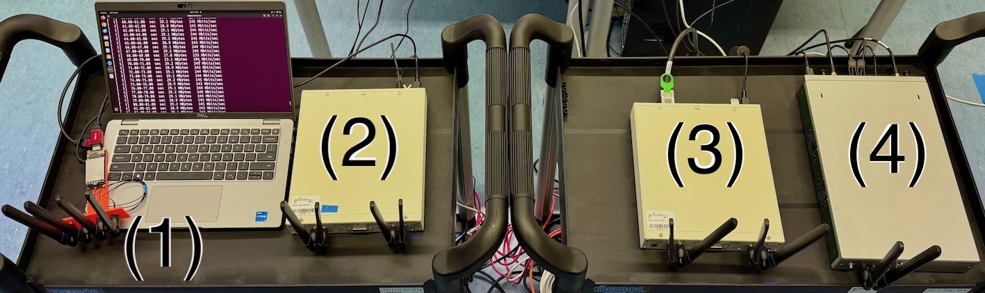
Figure 1: Experimental setup: (1) 5G UE and the SDR frontends for the (2) jammer, (3) watchdog, and (4) gNB. The corresponding PCs for (2–4) are not shown. The shown distances between the devices are for illustration purposes only. During experiments, the distance between adjacent devices was $1$ m.

The jammer and the watchdog run on separate computers, each using one USRP X310 [12] RF frontend. The jammer permanently transmits uniform noise signal of over the SSB subchannel at $f_{c}=3709.92$ MHz with $7.2$ MHz bandwidth. The watchdog permanently records IQ samples over $120$ MHz bandwidth to include the spectrum of the neighboring bands.

Dataset creation, training and measuring the classification time was performed on a single workstation with an Intel Xeon w7-2495X CPU and an NVIDIA RTX A6000 GPU. The operation system Ubuntu 22.04 LTS with Python 3.9.12 and keras 2.12.0 allowed to use all CPU cores during classification. The GPU was only used for training and is, thus, not utilized during the measurement of classification time.

II-B Dataset Creation

A spectrogram is composed as a stack of $n$ PSDs arrays. Each PSD array is obtained by applying an FFT to a window of $m$ IQ samples. We used an FFT rather than Welch’s method [13], sacrificing precision for computational speed. A spectrogram is then composed as a $n\times m$ matrix.

Based on previous measurement campaigns, we choose a window size of $m=1024$, leading to a frequency resolution of $117$ kHz and a stack of $n=100$ PSDs per spectrogram. This corresponds to a time window of $0.8$ ms.

The resulting spectrogram-matrices presented two problems when fed into the training set of the model. First, the power of received radio signals is very low in the linear domain and, thus, typically expressed in the logarithmic domain (decibel). Similarly, we apply the monotonic function $f(x)=-\log x$ to each value of the PSD array at each frequency, to avoid the vanishing gradient problem [14]. Second, due to approximation errors with very low energy bins, some values of the PSDs turned out to be $0$, which causes computation errors with the log function. Then used a small constant $\epsilon=10^{-21}$, leading to the applied transformation $f(x)=-\log(x+\epsilon)$. To each sample $i$, a label $y_{i}$ is assigned.

III Machine Learning Models

III-A Convolutional Neural Network

As spectrograms are two-dimensional, the first model of choice is a CNN whose structure is given in Table I. The objective is to return the correct label associated to each sample. The chosen loss function is the binary cross-entropy

$$L=-\frac{1}{N}\sum_{i=1}^{N}y_{i}\cdot\log(\tilde{y}_{i})+(1-y_{i})\cdot\log(1-\tilde{y}_{i}),$$ (1)

where $\tilde{y}_{i}$ is the prediction of the $i$-th sample. This function can approach infinity even if the prediction error cannot be above $1$, thus, allowing the model to update its weights.

TABLE I: Structure of the employed CNN

	Layer	Output size	No. of parameters
	Input	$100\times 1024\times 1$	$0$
	Convolutional 1	$49\times 511\times 32$	$320$
	Batch Normalization	$49\times 511\times 32$	$128$
	Average Pooling	$24\times 255\times 32$	$0$
	Convolutional 2	$22\times 253\times 64$	$18496$
	Batch Normalization	$22\times 253\times 64$	$256$
	Average Pooling	$11\times 126\times 64$	$0$
	Convolutional 3	$9\times 124\times 128$	$73856$
	Average Pooling	$4\times 62\times 128$	$0$
	Batch Normalization	$4\times 62\times 128$	$512$
	Flattening	$31744$	$0$
	Dense	$64$	$2031680$
	Dense	$32$	$2080$
	Dense	$16$	$528$
	Dense	$1$	$17$

Defining $\mathcal{C}_{0}$ as the class of no-jamming and $\mathcal{C}_{1}$ as the class of jamming, the jammer detection is performed by the following test function on the input sample $\bm{X}$ :

$$\hat{\mathcal{C}}=\begin{cases}\mathcal{C}_{0};&\tilde{y}_{i}<\tau,\\ \mathcal{C}_{1};&\tilde{y}_{i}\geq\tau,\\ \end{cases}$$ (2)

where $\tau$ is the chosen threshold. We, thus, measure accuracy as probability of false alarm (FA) and misdetection (MD) defined as

$$P_{\rm FA,C}={\mathbb{P}}[\hat{\mathcal{C}}=\mathcal{C}_{1}|\mathcal{C}=\mathcal{C}_{0}],$$ (3)

$$P_{\rm MD,C}={\mathbb{P}}[\hat{\mathcal{C}}=\mathcal{C}_{0}|\mathcal{C}=\mathcal{C}_{1}].$$ (4)

III-B Principal Component Analysis

Using $100\times 1024$ spectrograms as model input, leads to $102400$ dimensions. To avoid the curse of dimensionality, we reduce the number of coordinates in two steps.

First, we average spectrograms over time, reducing each $102400$-dimensional spectrogram to a $1024$-dimensional PSD. This filters out random fluctuations and yields robust PSDs.

Second, we further reduce the dimensions with principal component analysis (PCA). The basic idea of PCA is to change the basis so that the first coordinates (or principal components) contain “the most information” about the underlying data. The ratio of explained variance measures the information contained in each component and sums up to $1$, when summed over all components. The cumulated ratio of explained variance is displayed in Fig. 2. It can be seen that few components already capture most of the data’s information. In particular, 98%, 98.5% and 99% of the variance are explained by $8$, $13$ and $85$ principal components, respectively. This suggests $8$ components an optimal trade-off between computational complexity and accuracy.

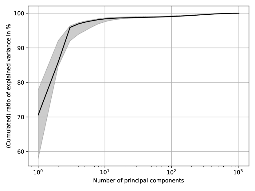
Figure 2: Cumulated ratio of explained variance in % for a varying number of principal components. The $0.01$- and $0.99$-quantiles are based on 100 random datasets and marked in gray

III-C $k$-Nearest Neighbors

For a new sample, KNN searches for the $k$ most similar samples from the training data and makes a prediction based on majority voting. The number of neighbors $k$ is a crucial hyperparameter that needs to be tuned. In Section IV-B results for a varying number of neighbors will be discussed.

KNN is sensitive to the scale of the data. To standardize the 1024-dimensional PSDs, we subtracted their respective means and divided the results by their respective standard deviations. We report results for (i) standardized PSDs and (ii) based on projections of non-standardized PSDs onto the first 8 principal components.

III-D Support Vector Machines

SVMs are a powerful class of machine learning models, which can be used for supervised classification and regression. SVMs operate by constructing a decision hyperplane in the feature space that optimally separates different classes. By employing the kernel trick, support vector machines can also be used effectively for non-linear tasks. In this work, we employed SVMs with varios kernels after dimension reduction with PCA.

III-E Classification Time

To measure how fast each of the above machine learning models can detect a jamming attack, we study classification time. This measure includes the computation time to compute the class and to apply the classification criterion. The time for computing the spectrogram from IQ samples is not included as it is equal for all machine learning models. In the following section, we will compare the cumulative distribution function (CDF) of the classification time obtained over $1000$ trials.

IV Experimental Results

IV-A Convolutional Neural Network

The training set was composed of $6000$ samples, equally distributed among the three cases described in Sec. II. Using the same distribution, the validation set was composed of $3000$ samples. This set is used to monitor the validation loss and to stop the training phase after three increases of the parameter. The test set contains $1200$ samples, distributed as the training and validation set.

Fig. 3 shows that the model perfectly distinguishes between the jamming and no-jamming cases. Fig. 4 shows the CDF of the classification time for a sample. In $95\%$ of the cases, a classification was achieved within $38$ ms.

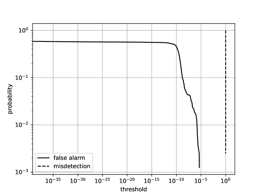
Figure 3: FA and MD probabilities as a function of the threshold $\tau\in[0,1]$ (with $y$ axis values normalized to $1$) for the considered jammer

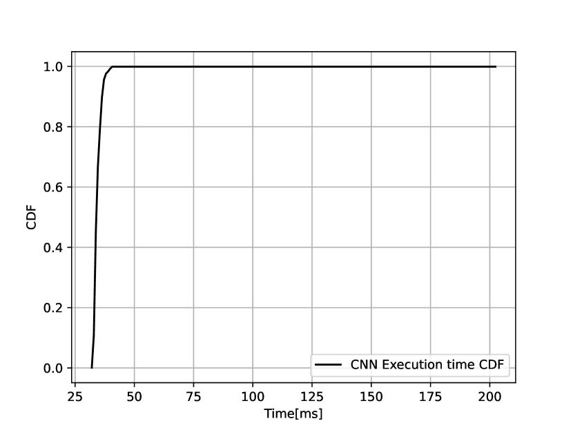
Figure 4: CDF of the classification time performed by the CNN with supervised learning

IV-B $k$-Nearest Neighbors

For each of the training, validation and test set, 1024 samples per class were selected from each of the three cases in Sec. II. The training, validation and test accuracy for the settings (i) standardized PSDs and (ii) based on projections of non-standardized PSDs onto the first 8 principal components are displayed in Table II. The optimal choice of neighbors based on the validation data is $k=8$ for setting (i) and $k=1$ for settings (ii). With an accuracy of approximately $99.98$%, we can reliably detect jammers.

Fig. 5 shows the CDF of the classification time of the KNN. With standardization, the model classified $95\%$ of the cases within $94$ ms. With PCA, the model performed substantially better with an classification time of $8$ ms for $95\%$ of the cases.

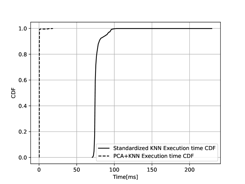
Figure 5: CDF of the classification time performed by the KNN with standardization and PCA

TABLE II: Classification accuracy with $k$-nearest neighbors in %

	Standardized			PCA (8 comp.)
$k$	training	validation	test	training	validation	test
1	100.000	96.754	96.717	100.000	99.996	99.979
2	99.987	99.988	99.980	99.985	99.995	99.974
4	99.983	99.988	99.979	99.985	99.995	99.976
8	99.981	99.989	99.978	99.985	99.995	99.975
10	99.981	99.989	99.977	99.985	99.995	99.975
20	99.981	99.984	99.975	99.985	99.995	99.972
30	99.981	99.983	99.972	99.985	99.992	99.968
40	99.980	99.980	99.967	99.985	99.988	99.962
50	99.977	99.979	99.960	99.985	99.981	99.959

IV-C Support Vector Machines

Our experiments with SVMs showed that this class of models is well suited to detecting jammers. The overall accuracy on the validation and test dataset significantly depends on the used kernel. We considered linear, polynomial and radial basis function (RBF) kernels. On the other hand, increasing the number of dimensions does not show a significant effect.

As shown in Table III, a large dimensionality reduction with a linear kernel produces models with high confidence scores over the datasets for validation and testing.

This large reduction of dimension, highly reduces the computational complexity of the classification. Fig. 6 shows that the SVM model classified 95% of the cases within $0.11$ ms. Thus, SVMs can detect jammers using substantially smaller computation time than the CNN (Fig. 4) and than the KNN without PCA (Fig. 5).

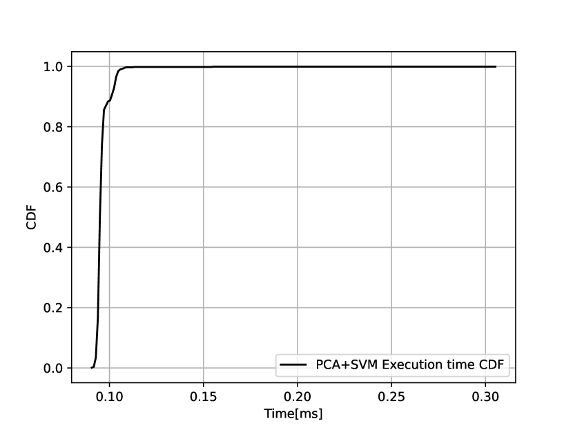
Figure 6: CDF of the classification time performed by the SVM with PCA

TABLE III: Classification accuracy with Support Vector Machines in $\%$

Kernel	Dim	Train Score	Val. Score	Test Score
linear	8	99.31	95.51	94.75
linear	13	99.63	93.52	93.04
linear	85	100	94.45	94.21
linear	full dataset	100	96.30	95.88
polynomial	8	98.60	98.20	98.01
polynomial	13	98.57	98.25	98.14
polynomial	85	98.57	98.20	98.14
polynomial	full dataset	99.99	98.98	98.73
rbf	8	98.66	98.66	98.45
rbf	13	98.66	98.74	98.39
rbf	85	98.63	98.77	98.40
rbf	full dataset	98.71	98.70	98.37

V Conclusion

We have compared three machine learning models to detect an SSB narrowband jammer in 5G networks. Based on data from an experimental 5G network, we studied the computation time and accuracy of these models.

From an accuracy point of view the three models yielded similar results, showing that they could distinguish between the two classes with $100\%$ accuracy in the CNN case and with more than $99.5\%$ accuracy in the other two cases.

The results for computation time are interesting due to their substantial differences. While the CNN required 38 ms to classify 95% of the cases, KNN needed only 8 ms if combined with PCA. The fasted classification was achieved by SVM with PCA, with a classification time of $0.11$ ms for 95% of the cases.

Based on these promising results, we will now study the robustness of the detection accuracy for various wireless network geometries and for multiple jamming signals.

References

- [1] L. Chettri and R. Bera, “A comprehensive survey on internet of things (IoT) toward 5G wireless systems,” IEEE Internet of Things Journal, vol. 7, no. 1, pp. 16–32, 2020.
- [2] H. Pirayesh and H. Zeng, “Jamming attacks and anti-jamming strategies in wireless networks: A comprehensive survey,” IEEE Communications Surveys & Tutorials, vol. 24, no. 2, pp. 767–809, Mar. 2022.
- [3] M. A. Birutis and A. Mykkeltveit, “Practical jamming of a commercial 5G radio system at 3.6 GHz,” in in Proc. International Conference on Military Communication and Information Systems (ICMCIS), vol. 205, 2022, pp. 58–67.
- [4] S. Hong, K. Kim, and S.-H. Lee, “A hybrid jamming detection algorithm for wireless communications: Simultaneous classification of known attacks and detection of unknown attacks,” IEEE Communications Letters, vol. 27, no. 7, pp. 1769–1773, 2023.
- [5] M. Hachimi, G. Kaddoum, G. Gagnon, and P. Illy, “Multi-stage jamming attacks detection using deep learning combined with kernelized support vector machine in 5G cloud radio access networks,” in 2020 International Symposium on Networks, Computers and Communications (ISNCC), 2020, pp. 1–5.
- [6] J. A. Jahanshahi, S. A. Ghorashi, and H. Sadreazami, “Jamming detection at base station using fuzzy c-means algorithm,” in in Proc. International Symposium on Computer Networks and Distributed Systems (CNDS), 2011, pp. 40–44.
- [7] Software Radio Systems, “SRS RAN documentation,” https://docs.srsran.com/en/latest/, accessed: 2024-04-19.
- [8] National Instruments, “USRP N300 datasheet,” https://www.ettus.com/all-products/usrp-n300/, accessed: 2024-04-19.
- [9] Quectel, “RM520-GL modem datasheet,” https://www.quectel.com/product/5g-rm520n-series, accessed: 2024-04-19.
- [10] S. Lee, “Open5GS documentation,” https://open5gs.org/open5gs/docs/, accessed: 2024-04-19.
- [11] 3GPP, “3GPP specification series 38: 5G standards,” https://www.3gpp.org/dynareport?code=38-series.htm, accessed: 2024-04-19.
- [12] Ettus, “USRPX 310 datasheet,” https://www.ettus.com/all-products/x310-kit/, accessed: 2024-04-19.
- [13] “Scipy welch periodogram,” https://docs.scipy.org/doc/scipy/reference/generated/scipy.signal.periodogram.html, accessed: 2024-04-19.
- [14] Z. Hu, J. Zhang, and Y. Ge, “Handling vanishing gradient problem using artificial derivative,” IEEE Access, vol. 9, pp. 22 371–22 377, 2021.