A velocity-based moving mesh Discontinuous Galerkin method for the advection-diffusion equation

Abstract

In convection-dominated flows, robustness of the spatial discretisation is a key property. While Interior Penalty Galerkin (IPG) methods already proved efficient in the situation of large mesh Peclet numbers, Arbitrary Lagrangian-Eulerian (ALE) methods are able to reduce the convection-dominance by moving the mesh. In this paper, we introduce and analyse a velocity-based moving mesh discontinuous Galerkin method for the solution of the linear advection-diffusion equation. By introducing a smooth parameterized velocity $\tilde{V}$ that separates the flow into a mean flow, also called moving mesh velocity, and a remaining advection field $V-\tilde{V}$, we made a convergence analysis based on the smoothness of the mesh velocity. Furthermore, the reduction of the advection speed improves the stability of an explicit time-stepping and the use of the nonconservative ALE formulation changes the coercivity condition. Finally, by adapting the existing robust error criteria to this moving mesh situation, we derived robust a posteriori error criteria that describe the potentially small deviation to the mean flow and include the information of a transition towards $V=\tilde{V}$.

65N15, 65N30

1 Introduction

Approaches to approximate advection phenomena with a moving mesh have been explored in several forms for a long time (e.g., [13] from 1974). The advection-dominance disappears and the scheme gains stability due to the reduction of the Courant number. In this landscape, the ALE approach that is based on a dynamic transformation map and that we can see at work for finite elements in the Lagrange-Galerkin method (see [2], [8], [9]) or with other forms of spatial discretisation, for finite volumes ([15]) or discontinuous Galerkin methods ([22]) has been combined successfully with error analysis ([2], [9]). Furthermore, the ALE-DG approach, which provides conservation properties [16], has already been discussed for problems with nonlinear diffusion ([1]) or in semi-Lagrangian methods for linear advection ([17]) and advection-diffusion ([3], [5]).

However, even after the advection-dominance has been removed or reduced, the presence of a small diffusion term and consequently a big mesh’s Peclet number $\frac{h}{\varepsilon}$ means that the space semi-discretisation still needs to be robust. Therefore, we need to preserve the robustness properties found in IPG ([21], [6] for complex geometries and diffusion tensor) or in its weighted version ([11], [4]). These approaches have given rise to robust a posteriori error estimates in order to develop adaptive mesh refinement (AMR) for the steady-state ([18]) or for the unsteady case ([7]).

In this paper we build a velocity-based moving mesh discontinuous Galerkin (DG) method that shows that taking precise account of what the deformation map does to the elliptic term preserves the convergence and robustness properties of the IPG. Since the smoothness of the deformation map is important in order to ensure the scheme’s convergence, we separate the advection field into a smooth mean flow with which the map moves and a remaining advection field that contains the small-scale deviations from the mean flow.

The a priori study of the error estimate shows that when possible, the maximal reduction of the advection term saves half an order of convergence for the spatial semi-discretisation. The a posteriori error estimate allows us to focus more closely on the elliptical term and to have a robust approach to the error. Finally, the test case involving a boundary layer problem shows that the ALE method makes it possible to get rid of the advection-dominance and focus on small-scale effects. This would not be possible with a static mesh method.

We consider the unsteady advection-diffusion equation:

(1) $$\begin{array}[]{ll}\frac{\partial u}{\partial t}+V\cdot\nabla u-\varepsilon\Delta u=f&[0,T]\times\Omega\vspace{1mm}\\ u=u_{D}&[0,T]\times\Gamma_{D}\vspace{1mm}\\ \varepsilon\frac{\partial u}{\partial n}=u_{N}&[0,T]\times\Gamma_{N}\vspace{1mm}\\ u(x,0)=u_{0}(x)&\Omega\end{array}$$

in a bounded space-time cylinder with a convex cross-section $\Omega\subset\mathbb{R}^{2}$, having a Lipschitz boundary $\Gamma$ consisting of two disjoint connected parts $\Gamma_{D}$ and $\Gamma_{N}$. The final time $T$ is arbitrary, but kept fixed in what follows. We assume that the data satisfy the following conditions:

(2) $$f\!\in\!C(0,T;L^{2}(\Omega)),\;u_{D}\!\in\!C(0,T;L^{2}(\Gamma_{D})),\;u_{N}\!\in\!C(0,T;L^{2}(\Gamma_{N})),$$

$$V\!\in\!C(0,T;W^{1,\infty}(\Omega)^{2}).$$

(3) $$0<\varepsilon\ll 1.$$

(4) $$\forall t\in[0,T],\;-\int_{\Omega}\nabla\cdot V(t,x)dx>0.$$

(5) $$\mbox{The Dirichlet boundary }\Gamma_{D}\mbox{ has a positive }1\mbox{-dimensional measure}$$

$$\mbox{and includes the inflow boundary }\{x\in\Gamma\hskip 1.42262pt|\hskip 1.42262ptV(t,x)\cdot\textbf{n}(x)<0\}\mbox{ for all }t.$$

Assumption (3) means that we are interested in the advection-dominated regime. Assumption (4) is necessary for the coercivity of the spatial operator so that (6) and (8) can be met.

In this formulation, $V$ is a prescribed velocity (for instance if (1) is the equation for the concentration of a chemical species, then $V$ is the velocity of the solute).

This equation will be reformulated with the help of a flowmap in section 2. In section 3 we introduce the DG semi-discretisation of equation (10), followed in section 4 of a study of an a priori error estimate in order to discuss the convergence of the method and an a posteriori error estimate in order to discuss the robustness, paving the way for AMR. Section 5 presents a boundary layer problem in order to demonstrate the properties of the method. Finally section 6 presents our conclusions.

In what follows, we will consider the case where $u_{D}=0$. For the case $u_{D}\neq 0$, we refer to remark 3.1.

2 Flow maps

We consider the ALE-DG method as a classical DG method defined on a deforming space. In this case, the complexity of the geometry occurring from the fact that the mesh moves will be featured in the equation itself. In order to do so, we define a smooth velocity $\tilde{V}\in C(0,T;W^{1,\infty}(\Omega))$ s.t.

(6) $$\tilde{V}\!\cdot\!\textbf{n}=0\mbox{ on }\Gamma\times[0,T]$$

(7) $$\tilde{V}=0\mbox{ on }\Gamma_{D}\cap\Gamma_{N}$$

(8) $$-\frac{1}{2}\nabla\!\cdot\!(V(t,x)-\tilde{V}(t,x))=\beta(t)>0$$

(9) $$\lVert\nabla\!\cdot\!(V(t,x)-\tilde{V}(t,x))\rVert\leq c_{*}\beta$$

for a constant $c_{*}$ independent of time. The existence of such a function $\tilde{V}$ is ensured by assumption (7). We also decide that $\tilde{V}$ vanishes on the boundary between $\Gamma_{N}$ and $\Gamma_{D}$. Assumption (6) is necessary to insure that the computational domain does not change.

We introduce the flow map to distinguish a Lagrangian (or reference) variable $X$ and an Eulerian (or spatial) variable $x$. $X$ lives in a space $\Omega_{r}$ that is later defined (and $x$ lives in $\Omega$). We carry out all the computations in $\Omega_{r}$ and express them back in $\Omega$.

Given $\tilde{V}$ the associated flow map, $x=\chi(t,X)$, satisfies:

$\dot{x}(t,X)=\tilde{V}(t,x(t,X))$,     $x(0,X)=X$

As $\tilde{V}$ is smooth we have $\chi(t,.):\Omega_{r}\rightarrow\Omega$ is a $C^{1}$-diffeomorphism and the Jacobian $F=F(t,X)=[\frac{\partial x_{i}}{\partial X_{j}}]_{i,j}$ satisfies:

$\dot{F}(t,X)=(\nabla\tilde{V}(t,x))F(t,X)$,     $F(0,X)=I$,     $x=\chi(t,X)$.

The determinant $J=\mbox{det}(F)$ satisfies $\dot{J}=J(\nabla\!\cdot\!\tilde{V})$.

For a fixed domain $\Omega_{r}=\Omega$ with Lipschitz boundary $\Gamma_{r}=\Gamma$ let $\Omega(t)=\chi(t,\Omega_{r})$. The unit normal outward $\textbf{n}_{r}=\textbf{n}_{r}(X)$ to $\Gamma_{r}$ and the unit normal outward $\textbf{n}=\textbf{n}(t,x)$ to $\Gamma$ are related by the formula:

$\textbf{n}(t,x)=\left(\frac{F^{-T}\textbf{n}_{r}}{|F^{-T}\textbf{n}_{r}|}\right)(t,X)$,     $X\in\partial\Omega_{r}$,     $x=\chi(t,X)$.

Because of the value of $\tilde{V}$ on $\Gamma_{r}$, $\Omega_{r}=\Omega(t)=\Omega$, $\chi(t,\Gamma_{D})=\Gamma_{D}$ and $\chi(t,\Gamma_{N})=\Gamma_{N}$.

For any function $v(t,x)$ we introduce the $\hat{}$-notation s.t. $\hat{v}(t,X)=v(t,x(t,X))$ and reciprocally $v$ can be defined thanks to $\hat{v}$. This notation also stands for functions independent of time, $\hat{v}(t,X)=v(x)$ and $v(t,x)=\hat{v}(X)$.

Then: $\hat{v}_{t}=v_{t}+\tilde{V}\cdot\nabla v,$ $\nabla v=F^{-T}\nabla_{X}\hat{v}$ and $\Delta v=\frac{1}{J}\nabla_{X}\cdot(JF^{-1}F^{-T}\nabla_{X}\hat{v}).$

When writing $\hat{f}(t,X)=f(t,x(t,X)),$ $\hat{u}_{D}(t,X)=u_{D}(t,x),$ $\hat{u}_{N}(t,X)=u_{N}(t,x),$ and $\hat{u}_{0}(X)=u_{0}(x(0,X))$, the PDE in (1) can now be written in the moving framework, using $\tilde{V}$ as the deformational flow:

(10) $$\frac{\partial\hat{u}}{\partial t}+(V-\tilde{V})\!\cdot\!F^{-T}\nabla_{X}\hat{u}-\frac{\varepsilon}{J}\nabla_{X}\!\cdot\!\{JF^{-1}F^{-T}\nabla_{X}\hat{u}\}=\hat{f}$$

In the following we will discretise (10) with a DG method in space. This approach allows us to compute the approximation on the static space $\Omega_{r}$ with a partition $\mathcal{T}_{h}$ defined later.

3 The semi-discrete interior penalty discretisation formulation for the unsteady advection-diffusion equation

In this section we will discuss the DG formulation of (10). We start with the weak form of the equations and define the semi-discrete problem in the first two subsections that leads to the definition of the discrete variational problem (14). Some properties of the operators used for the semi-discretisation are stated in subsection 3.3, they show the well-posedness of our problem and open the way for the error estimates that will be discussed in section 4.

3.1 Notation and weak form

Let $\omega_{r}\subset\Omega_{r}$, we define the following:

$$\lVert\hat{v}\rVert^{2}_{H_{\omega_{r}}(t)}=\int_{\omega_{r}}\hat{v}^{2}J(t,\!\cdot\!),\hskip 8.53581pt|\hat{v}|^{2}_{U_{\omega_{r}}(t)}=\int_{\omega_{r}}(\nabla_{X}\hat{v})^{T}F(t,\!\cdot\!)^{-1}F(t,\!\cdot\!)^{-T}(\nabla_{X}\hat{v})J(t,\!\cdot\!)$$

If $\omega_{r}=\Omega_{r}$, the index $\Omega_{r}$ is omitted. Denoting $v(t,\chi(t,X))=\hat{v}(X)$, $\omega(t)=\chi(t,\omega_{r})$,

$$\lVert v\rVert_{L^{2}(\omega)}=\lVert\hat{v}\rVert_{H_{\omega_{r}}(t)}\mbox{ and }|v|_{H^{1}(\omega)}=|\hat{v}|_{U_{\omega_{r}}(t)}.$$

The equalities show that the metrics can be constructed within the framework of the reference variable $X$: by denoting $e$ the approximation error, the bounds on $\|\hat{e}\|_{H(t)}$ and $|\hat{e}|_{U(t)}$ represent $L^{2}$- and $H^{1}$-bounds on $e$.

We define the spaces $L^{p}(0,T;Z)$ (with $Z$ a Banach space) that consist of mesurable functions $v\colon[0,T]\rightarrow Z$ for which:

$$\lVert v\lVert_{L^{p}(0,T;Z)}^{p}=\int_{0}^{T}\lVert v(t)\rVert_{Z}^{p}dt<+\infty\mbox{ for }1\leq p<+\infty$$

$$\lVert v\rVert_{L^{\infty}(0,T;Z)}=\underset{0\leq t\leq T}{\mbox{ess sup}}\lVert v(t)\rVert_{Z}<+\infty\mbox{ for }p=+\infty$$

Set $H^{1}_{D}(\Omega_{r})\!=\!\{\hat{v}\in H^{1}(\Omega_{r})\colon\hat{v}=0\mbox{ on }\Gamma_{D}\}$.

For $\hat{u},\hat{v}\in H^{1}(\Omega_{r})$ we define the following:

$$a(\hat{u},\hat{v})=\int_{\Omega_{r}}J[\varepsilon(F^{-T}\nabla_{X}\hat{u})\!\cdot\!(F^{-T}\nabla_{X}\hat{v})+(V-\tilde{V})\!\cdot\!(F^{-T}\nabla_{X}\hat{u})\hat{v}]$$

$$l(\hat{v})=\int_{\Omega_{r}}J\hat{f}\hat{v}+\int_{\Gamma_{N}}\hat{u}_{N}\hat{v}|F^{-T}\textbf{n}_{r}|$$

With these definitions the weak formulation of (10) becomes:

(11) $$\mbox{Find }\hat{u}\in L^{2}(0,T;H_{D}^{1}(\Omega_{r}))\cap C^{1}(0,T;H^{-1}(\Omega_{r}))\\ \mbox{ s.t. }\forall t\in[0,T],\,\forall\hat{v}\in H_{D}^{1}(\Omega_{r})\hskip 5.69054pt\int_{\Omega_{r}}J\frac{\partial\hat{u}}{\partial t}\hat{v}=l(\hat{v})-a(\hat{u},\hat{v})$$

Integration by parts then yields

$$a(\hat{u},\hat{v})=\int_{\Omega_{r}}J[\varepsilon(F^{-T}\nabla_{X}\hat{u})\!\cdot\!(F^{-T}\nabla_{X}\hat{v})-\hat{u}(V-\tilde{V})\!\cdot\!(F^{-T}\nabla_{X}\hat{v})-\nabla\!\cdot\!(V-\tilde{V})\hat{u}\hat{v}]\\ +\int_{\Gamma_{N}}J(V-\tilde{V})\!\cdot\!(F^{-T}\textbf{n}_{r})\hat{u}\hat{v}$$

The formulation (11) is a nonconservative weak ALE formulation for problem (1). Regularity of the ALE map $\chi$ guarantees the parabolic nature of the resulting equation and consequently the existence of a unique solution to (11).

3.2 Bilinear forms and function spaces for the semi-discretisation

To discretise (11), we consider regular and shape-regular meshes $\mathcal{T}_{h}=\{K\}$ that partition the computational domain $\Omega_{r}$ into open triangles. We consider this mesh to be static and steady. For simplicity we assume that $\Omega_{r}$ is a polyhedron that is covered exactly by $\mathcal{T}_{h}$. We assume the following:

(i) The elements of $\mathcal{T}_{h}$ satisfy the minimal angle condition. Specifically, there is a constant $\xi_{0}>0$ such that $\frac{h_{K}}{r_{K}}<\xi_{0}$ where $h_{K}$ and $r_{K}$ denote, respectively, the diameters of the circumscribed and inscribed balls to $K$.

(ii) $\mathcal{T}_{h}$ is locally quasi-uniform; that is, if two elements $K_{1}$ and $K_{2}$ are adjacent in the sense that $\mu_{d-1}(\partial K_{1}\cap\partial K_{2})>0$ then $\mbox{diam}(K_{1})\approx\mbox{diam}(K_{2})$.

Here $\mu_{d-1}$ denotes the $(d-1)$-dimensional Lebesgue measure. Let $h_{E}$ be the size of an edge $E$.

Given the discontinuous nature of the piecewise polynomial functions, let the sets of edges:

$$\mathcal{E}^{\mbox{\tiny int}}\!=\!\{e\!=\!\partial\!K_{1}\!\cap\!\partial\!K_{2}\colon\mu_{d-1}(\partial\!K_{1}\!\cap\!\partial\!K_{2})\!>\!0\},\,\mathcal{E}^{\mbox{\tiny ext}}\!=\!\{e\!=\!\partial\!K\!\cap\!\Gamma\colon\mu_{d-1}(\partial\!K\!\cap\!\Gamma)>0\},$$

$$\mathcal{E}_{N}^{\mbox{\tiny ext}}=\!\{e\!=\!\partial\!K\!\cap\!\Gamma_{N}\colon\mu_{d-1}(\partial\!K\!\cap\!\Gamma_{N})\!>\!0\},\,\mathcal{E}_{D}^{\mbox{\tiny ext}}\!=\!\{e\!=\!\partial\!K\!\cap\!\Gamma_{D}\colon\mu_{d-1}(\!\partial\!K\!\cap\!\Gamma_{D})\!>\!0\},$$

$$\mathcal{E}=\mathcal{E}^{\mbox{\tiny ext}}(\mathcal{T}_{h})\cup\mathcal{E}^{\mbox{\tiny int}}(\mathcal{T}_{h}),\,\mathcal{E}_{N}=\mathcal{E}_{N}^{\mbox{\tiny ext}}(\mathcal{T}_{h})\cup\mathcal{E}^{\mbox{\tiny int}}(\mathcal{T}_{h})\mbox{ and }\mathcal{E}_{D}=\mathcal{E}_{D}^{\mbox{\tiny ext}}(\mathcal{T}_{h})\cup\mathcal{E}^{\mbox{\tiny int}}(\mathcal{T}_{h}).$$

We write $\textbf{n}_{K}$ the outward unit normal vector on the boundary $\partial K$ of an element $K$ and for a set of points $Y$ the set of elements $K$ containing $Y$: $\omega_{Y}=\underset{K\cap Y\neq\emptyset}{\cup}K$.

Let the inflow and outflow boundaries of $\partial\Omega$

$\Gamma_{\mbox{\tiny in}}^{t}=\{x\in\Gamma\colon(V-\tilde{V})\!\cdot\!F^{-T}\textbf{n}<0\}$, and $\Gamma_{\mbox{\tiny out}}^{t}=\{x\in\Gamma\colon(V-\tilde{V})\!\cdot\!F^{-T}\textbf{n}\geq 0\}$

Similarly, the inflow and outflow boundaries of an element K are defined by

$\partial K_{\mbox{\tiny in}}^{t}=\{x\in\partial K\colon(V-\tilde{V})\!\cdot\!F^{-T}\textbf{n}_{K}<0\}$, $\partial K_{\mbox{\tiny out}}^{t}=\{x\in\partial K\colon(V-\tilde{V})\!\cdot\!F^{-T}\textbf{n}_{K}\geq 0\}$.

The broken Sobolev spaces and the space of piecewise polynomials associated with $\mathcal{T}_{h}$

$$H^{k}\!(\mathcal{T}_{h})\!=\!\{\varphi\!\in\!L^{2}\!(\Omega_{r})\!\colon\!\forall K\!\in\!\mathcal{T}_{h}\;\varphi|_{K}\!\in\!H^{k}\!(K)\},\;V_{h}\!=\!\{\varphi\!\in\!H^{1}\!(\mathcal{T}_{h})\!\colon\!\forall K\!\in\!\mathcal{T}_{h}\;\varphi|_{K}\!\in\!\mathcal{S}_{p}\!(K)\}$$

with $\mathcal{S}_{p}$ the space of polynomials of degree $\leq p$. We suppose $p\geq 1$.

Finally $U_{h}=V_{h}+H_{D}^{1}(\Omega_{r})$ and $V_{h}^{c}=V_{h}\cap H_{D}^{1}(\Omega_{r})$.

The jumps and averages of functions in $H^{1/2}(\mathcal{T}_{h})$ are defined as follows. Let the edge $E\in\mathcal{E}^{\mbox{\tiny int}}$ be shared by two neighboring elements $K$ and $K^{e}$. For ${\hat{v}\in H^{1/2}(\mathcal{T}_{h})}$, $\hat{v}|_{E}$ its trace on $E$ taken from inside $K$, and $\hat{v}^{e}|_{E}$ the one taken inside $K^{e}$. The jump of $\hat{v}$ and the average of a vector field $\textbf{q}\in H^{1/2}(\mathcal{T}_{h})^{d}$ across the edge $E$ are then defined

$$[\![\hat{v}]\!]\!=\!\left\{\begin{array}[]{ll}\hat{v}|_{E}\textbf{n}_{K}\!+\!\hat{v}^{e}|_{E}\textbf{n}_{K^{e}}&\mbox{for }E\!\in\!\mathcal{E}^{\mbox{\tiny int}}\\ \hat{v}|_{E}\textbf{n}_{r}&\mbox{for }E\!\in\!\mathcal{E}^{\mbox{\tiny ext}}\end{array}\right.\mbox{ and }\{\!\{\textbf{q}\}\!\}\!=\!\left\{\begin{array}[]{ll}\frac{1}{2}(\textbf{q}|_{E}\!+\!\textbf{q}^{e}|_{E})&\mbox{for }E\!\in\!\mathcal{E}^{\mbox{\tiny int}}\\ \textbf{q}|_{E}&\mbox{for }E\!\in\!\mathcal{E}^{\mbox{\tiny ext}}\end{array}\right.$$

Remark 3.1.

The definition of the jump holds for $u_{D}=0$, when we consider the general case we modify the definition of the jump: $[\![\hat{v}]\!]\!=\!(\hat{v}|_{E}-\hat{u}_{D})\textbf{n}_{r}\mbox{ for }E\!\in\!\mathcal{E}_{D}^{\mbox{\tiny ext}}$.

Additionally we define $a_{h}(\cdot,\cdot)$ as

(12) $$a_{h}(\hat{u},\hat{v})=\underset{K\in\mathcal{T}_{h}}{\sum}\int_{K}J[\varepsilon(F^{-T}\nabla_{X}\hat{u})\!\cdot\!(F^{-T}\nabla_{X}\hat{v})+(V-\tilde{V})\!\cdot\!(F^{-T}\nabla_{X}\hat{u})\hat{v}]\\ -\underset{E\in\mathcal{E}_{D}}{\sum}\int_{E}J^{\frac{1}{2}}\varepsilon(\{\!\{\Pi_{L^{2}}(J^{\frac{1}{2}}F^{-T}\nabla_{X}\hat{u})\}\!\}\!\cdot\!F^{-T}[\![\hat{v}]\!]+\theta\{\!\{\Pi_{L^{2}}(J^{\frac{1}{2}}F^{-T}\nabla_{X}\hat{v})\}\!\}\!\cdot\!F^{-T}[\![\hat{u}]\!])\\ +\frac{\alpha\varepsilon}{h_{E}}\int_{E}JF^{-T}[\![\hat{u}]\!]\!\cdot\!F^{-T}[\![\hat{v}]\!]-\underset{K\in\mathcal{T}_{h}}{\sum}\int_{\partial K_{\mbox{\tiny in}}^{t}}J(V-\tilde{V})\!\cdot\!(F^{-T}[\![\hat{u}]\!])\hat{v}$$

$\alpha>0$ is the interior penalty parameter increases with the polynomial degree, let $\theta\in\{-1,1\}$, the method is called symmetric interior penalty (SIPG) when $\theta=1$ and nonsymmetric interior penalty (NIPG) when $\theta=-1$. $\Pi_{L^{2}}$ denotes the elementwise orthogonal $L^{2}$-projection onto the finite element space $(V_{h})^{2}$, it has the property

(13) $$\forall\hat{g}\in(L^{2}(\Omega_{r}))^{2},\;\|\Pi_{L^{2}}\hat{g}\|_{L^{2}(\Omega_{r})}\leq\|\hat{g}\|_{L^{2}(\Omega_{r})}$$

The DG method is based on an upwind discretisation for the convective term and a (non-)symmetric interior penalty discretisation for the Laplacian, is formulated as

(14) $$\mbox{Find }\hat{u}_{h}\!\in\!C^{1}\!(0,T;V_{h})\mbox{ s.t. }\forall t\!\in\![0,T],\forall\hat{v}_{h}\!\in\!V_{h}\;\int_{\Omega_{r}}\!J\frac{\partial\hat{u}_{h}}{\partial t}\hat{v}_{h}\!=\!l_{h}(\hat{v}_{h})\!-\!a_{h}(\hat{u}_{h},\!\hat{v}_{h})\\ \mbox{where }\hat{u}_{h}(0,\cdot)\in V_{h}\mbox{ is a projection of }\hat{u}_{0}(\cdot)\mbox{ onto $V_{h}$.}$$

$$\mbox{With }l_{h}(\hat{v})=\underset{K\in\mathcal{T}_{h}}{\sum}\int_{K}\hat{f}\hat{v}+\underset{E\in\mathcal{E}_{N}^{\mbox{\tiny ext}}}{\sum}\int_{E}\hat{u}_{N}\hat{v}.\\$$

Finally, for $\hat{u},\hat{v}\in H^{1}(\mathcal{T}_{h})$

$$d_{h}(\hat{u},\hat{v})= \!\underset{K\in\mathcal{T}_{h}}{\sum}\int_{K}J\varepsilon(F^{-T}\nabla_{X}\hat{u})\!\cdot\!(F^{-T}\nabla_{X}\hat{v})-\hat{u}\hat{v}\nabla_{x}\!\cdot\!(V-\tilde{V})$$

$$f_{h}(\hat{u},\hat{v})= -\underset{K\in\mathcal{T}_{h}}{\sum}\int_{K}J(V-\tilde{V})\!\cdot\!(F^{-T}\nabla_{X}\hat{v})\hat{u}+\underset{K\in\mathcal{T}_{h}}{\sum}\int_{\partial K_{\mbox{\tiny out}}^{t}}J(V-\tilde{V})\!\cdot\!F^{-T}[\![\hat{v}]\!]\hat{u}$$

$$j_{h}(\hat{u},\hat{v})= \!\underset{E\in\mathcal{E}_{D}}{\sum}\int_{E}\frac{\alpha}{h_{E}}JF^{-T}[\![\hat{u}]\!]\!\cdot\!F^{-T}[\![\hat{v}]\!]$$

$$\tilde{a}_{h}(\hat{u},\hat{v})= d_{h}(\hat{u},\hat{v})+f_{h}(\hat{u},\hat{v})+\varepsilon j_{h}(\hat{u},\hat{v})$$

$$\tilde{p}_{h}(\hat{u},\hat{v})= \!\underset{E\in\mathcal{E}_{D}}{\sum}\!\int_{E}\!J^{\frac{1}{2}}\!\varepsilon(\!\{\!\{\Pi_{L^{2}}(J^{\frac{1}{2}}\!F^{-T}\nabla\!_{X}\hat{u})\}\!\}\!\cdot\!F^{-T}\![\![\hat{v}]\!]\!+\!\theta\!\{\!\{\Pi_{L^{2}}(J^{\frac{1}{2}}F^{-T}\!\nabla\!_{X}\hat{v})\}\!\}\!\cdot\!F^{-T}\![\![\hat{u}]\!])$$

Integration by parts then gives:

(15) $$a_{h}(\hat{u},\hat{v})=\tilde{a}_{h}(\hat{u},\hat{v})-\tilde{p}_{h}(\hat{u},\hat{v})$$

3.3 Properties of the bilinear operator

In this subsection we state some properties of the operators. The coercivity lemma proves the stability of the method. Convergence cannot be shown directly since the operator is inconsistent, but the inconsistency lemma will be useful in the proof of the a priori error theorem 4.1. The convergence of the method is then subject to the conditions described in remark 4.3. The continuity and inf-sup condition lemmas show well-posedness and will be useful for the development of a posteriori error estimates. Before the development of these properties, we will recall some classical tools for studying finite element discretisations as well as the norms and semi-norms used for analysing the semi-discretisation.

By (3.41) in [12] there exist inverse and trace inequalities for the Eulerian framework.

(16) $$\lVert\hat{v}_{h}\rVert_{\partial K}^{2} \leq C_{T}h_{K}^{-1}\lVert\hat{v}_{h}\rVert_{K}^{2}$$

(17) $$\lVert\nabla_{X}\hat{v}_{h}\rVert_{K} \leq C_{I}h_{K}^{-1}\lVert\hat{v}_{h}\rVert_{K}$$

$C_{T}>0$ and $C_{I}>0$ depend on the polynomial degree.

To analyse the spatial error in (21) and in the criteria (48), let $g_{q}^{\omega_{r}}=\frac{\lVert g\rVert_{L^{q}(\omega_{r})}}{\omega_{r}^{q}}$ for $\omega_{r}\subset\Omega_{r}$, $q\in[1,\infty]$ and $g\in L^{p}(\omega_{r})$ with $\omega_{r}^{q}$ the $L^{q}$-norm of the indicator function of $\omega_{r}$. For instance $\omega_{r}^{1}$ is the Lebesgue measure of $\omega_{r}$. And we write

(18) $$\delta\!=\!(V-\tilde{V})^{2},\,M\!=\!\frac{1}{J}\mbox{ and }a\mbox{ the pointwise maximal eigenvalue of }JF^{-1}F^{-T}$$

In what follows we will often use that since $\det(JF^{-1}F^{-T})=1$ and $d=2$, the maximal eigenvalue of $JF^{-1}F^{-T}$ is the same as the maximal eigenvalue of $J^{-1}F^{T}F$.

We define the norms

(19) $$\forall\hat{v}\in H^{1}(\mathcal{T}_{h}),\;|||\hat{v}|||^{2} =\underset{K\in\mathcal{T}_{h}}{\sum}[\varepsilon|\hat{v}|_{U_{K}}^{2}+\beta\lVert\hat{v}\rVert^{2}_{H_{K}}]+\varepsilon j_{h}(\hat{v},\hat{v})$$

(20) $$\forall\textbf{q}\in H^{0}(\Omega_{r})^{d},\;|\textbf{q}|_{*} =\underset{\hat{v}\in H^{1}_{D}(\Omega_{r})-\{0\}}{\mbox{sup}}\frac{1}{|||\hat{v}|||}\int_{\Omega_{r}}J\textbf{q}\cdot F^{-T}\nabla_{X}\hat{v}$$

(21) $$\forall\hat{v}\in H^{1}(\mathcal{T}_{h}),\;|\hat{v}|^{2}_{A} =|(V-\tilde{V})\hat{v}|^{2}_{*}+\underset{E\in\mathcal{E}_{D}}{\sum}(\beta+\frac{\delta_{\infty}^{\omega_{E}}}{\varepsilon})h_{E}J_{1}^{\omega_{E}}\int_{E}[\![\hat{v}]\!]^{2}$$

The first norm is the DG-norm associated with the discretisation of (10). The seminorm $|\cdot|_{*}$ is linked to the Helmholtz decomposition, in particular q is called divergence-free when $|\textbf{q}|_{*}=0$ holds. The third norm measures the error of the transport behaviour.

Finally we define the notation $\lesssim$ as a bound that is valid up to a constant that is independent of the local mesh size $h$, diffusion coefficient $\varepsilon$ and speed $\delta$.

Lemma 3.2.

(Coercivity) For $\alpha$ large enough (depending on the value of the scalar $C_{T}$ in the inverse trace inequality (16)) $a_{h}$ is $|||\cdot|||$-coercive. For all $\hat{v}_{h}\in U_{h}$

(22) $$|||\hat{v}_{h}|||^{2}\lesssim a_{h}(\hat{v}_{h},\hat{v}_{h})$$

Proof 3.3.

Let $\hat{v}_{h}\in V_{h}$, by noticing that $a_{h}=\frac{1}{2}(\mbox{ \eqref{bilin:Ah} }+\mbox{ \eqref{bilin:Ahint} })$:

$$a_{h}(\hat{v}_{h},\hat{v}_{h})\geq\frac{\beta}{2}\underset{K\in\mathcal{T}_{h}}{\sum}||\hat{v}_{h}||_{H_{K}}^{2}+\varepsilon(j_{h}(\hat{v}_{h},\hat{v}_{h})+\underset{K\in\mathcal{T}_{h}}{\sum}|\hat{v}_{h}|_{U_{K}}^{2})-\tilde{p}_{h}(\hat{v}_{h},\hat{v}_{h})$$

If $\theta=-1$, then $\tilde{p}_{h}(\hat{v}_{h},\hat{v}_{h})=0$, thus $a_{h}(\hat{v}_{h},\hat{v}_{h})\geq\frac{1}{2}|||\hat{v}_{h}|||^{2}$.

When $\theta=1$, using successively Young’s inequality, (16), (13) and (17), we obtain

$$2\underset{E\in\mathcal{E}_{D}}{\sum}\int_{E}\{\!\{\Pi_{L^{2}}(J^{\frac{1}{2}}F^{-T}\nabla\hat{v}_{h})\}\!\}\cdot J^{\frac{1}{2}}F^{-T}[\![\hat{v}_{h}]\!]\leq\sqrt{\frac{C_{T}}{\alpha}}(j_{h}(\hat{v}_{h},\hat{v}_{h})+\underset{K\in\mathcal{T}_{h}}{\sum}|\hat{v}_{h}|_{U_{K}}^{2}).$$

$$\mbox{Thus }|||\hat{v}_{h}|||^{2}\leq\max{(2,(1-\sqrt{\frac{C_{T}}{\alpha}})^{-1})}a_{h}(\hat{v}_{h},\hat{v}_{h}),\mbox{ that is bounded for }\alpha>C_{T}.$$

As often used in the literature, we will suppose that $\alpha\geq 2C_{T}$.

Lemma 3.4.

(Inconsistency) Let $\hat{u}\in C^{1}(0,T;H^{1}(\Omega_{r}))$ be an analytical solution of (10), $\hat{u}_{h}$ solve (14) and $\hat{e}=\hat{u}-\hat{u}_{h}$. Then $\forall\hat{v}_{h}\in V_{h}$

$$\int_{\Omega_{r}}J\frac{\partial\hat{e}}{\partial t}\hat{v}_{h}+a_{h}(\hat{e},\hat{v}_{h})\!=\!\varepsilon\underset{E\in\mathcal{E}_{D}}{\sum}\int_{E}\{\!\{J^{\frac{1}{2}}F^{-T}\nabla_{X}\hat{u}-\Pi_{L^{2}}(J^{\frac{1}{2}}F^{-T}\nabla_{X}\hat{u})\}\!\}\cdot J^{\frac{1}{2}}F^{-T}[\![\hat{v}_{h}]\!]\\$$

Proof 3.5.

Let $\hat{v}_{h}\in V_{h}$, with (12) , $\hat{u}(t,\cdot)\in H^{1}(\Omega_{r})$ and integration by parts:

$$\int_{\Omega_{r}} J\frac{\partial\hat{u}}{\partial t}\hat{v}_{h}\!+\!a_{h}(\hat{u},\hat{v}_{h})\!=\!\underset{K\in\mathcal{T}_{h}}{\sum}\int_{K}(J(V-\tilde{V})\!\cdot\!F^{-T}\nabla_{X}\hat{u}-\varepsilon\nabla_{X}\!\cdot\!\{JF^{-1}F^{-T}\nabla_{X}\hat{u}\})\hat{v}_{h}$$

$$+\varepsilon\int_{\partial K}JF^{-1}F^{-T}\nabla_{X}\hat{u}\cdot\textbf{n}_{r}\hat{v}_{h}-\varepsilon\underset{E\in\mathcal{E}_{D}}{\sum}\int_{E}\{\!\{\Pi_{L^{2}}(J^{\frac{1}{2}}F^{-T}\nabla_{X}\hat{u})\}\!\}\cdot J^{\frac{1}{2}}F^{-T}[\![\hat{v}_{h}]\!]$$

$$=\! \int_{\Omega_{r}}\!J\frac{\partial\hat{u}_{h}}{\partial t}\hat{v}_{h}\!+\!a_{h}(\hat{u}_{h},\!\hat{v}_{h})\!+\!\varepsilon\!\underset{E\in\mathcal{E}_{D}}{\sum}\int_{E}\{\!\{\!J^{\frac{1}{2}}\!F^{-T}\!\nabla_{X}\hat{u}\!-\!\Pi_{L^{2}}\!(J^{\frac{1}{2}}\!F^{-T}\!\nabla_{X}\hat{u})\!\}\!\}\!\cdot\!J^{\frac{1}{2}}\!F^{-T}[\![\hat{v}_{h}]\!]$$

The last equality follows from (10) and (14).

Lemma 3.6.

(Continuity) For $\hat{v}\in H^{1}_{D}(\Omega_{r})$, $\hat{w}_{1},\hat{w}_{2}\in U_{h}$, the following properties hold:

(23) $$|d_{h}(\hat{w}_{1},\hat{w}_{2})| \leq\max(1,c_{*})|||\hat{w}_{1}|||\cdot|||\hat{w}_{2}|||,$$

(24) $$|j_{h}(\hat{w}_{1},\hat{w}_{2})| \leq|||\hat{w}_{1}|||\cdot|||\hat{w}_{2}|||,$$

(25) $$|f_{h}(\hat{w}_{1},\hat{v})| \leq|(V-\tilde{V})\hat{w}_{1}|_{*}\cdot|||\hat{v}|||.$$

Proof 3.7.

(23) and (24) follow from the Cauchy-Schwarz inequality and (9).

$$|f_{h}(\hat{w}_{1},\hat{v})| \leq|\underset{K\in\mathcal{T}_{h}}{\sum}\int_{K}\hat{w}_{1}J(V-\tilde{V})\cdot F^{-T}\nabla_{X}\hat{v}|\leq|||\hat{v}|||\frac{|\int_{\Omega_{r}}\hat{w}_{1}J(V-\tilde{V})\cdot F^{-T}\nabla_{X}\hat{v}|}{|||\hat{v}|||}$$

$$\leq|(V-\tilde{V})\hat{w}_{1}|_{*}\cdot|||\hat{v}|||$$

Lemma 3.8.

(Inf-Sup) $\tilde{a}_{h}$ satisfies the following condition:

$$\underset{\hat{v}\in H_{D}^{1}(\Omega_{r})-\{0\}}{\inf}\underset{\hat{w}\in H_{D}^{1}(\Omega_{r})-\{0\}}{\sup}\frac{\tilde{a}_{h}(\hat{v},\hat{w})}{(|||\hat{v}|||+|(V-\tilde{V})\hat{w}|_{*})\cdot|||\hat{w}|||}\geq C>0$$

Proof 3.9.

Let $\hat{v}\in H^{1}_{D}(\Omega_{r})-\{0\}$ and $\sigma\in]0;1[$. Then by definition of the norm $|\cdot|_{*}$ there exists $\hat{w}_{\sigma}\in H^{1}_{D}(\Omega_{r})$ s.t. $|||\hat{w}_{\sigma}|||=1$ and

$$f_{h}(\hat{v},\hat{w}_{\sigma})=-\int_{\Omega_{r}}J\hat{v}(V-\tilde{V})\cdot F^{-T}\nabla_{X}\hat{w}_{\sigma}\geq\sigma|(V-\tilde{V})\hat{v}|_{*}.$$

$$\mbox{Then }\tilde{a}_{h}(\hat{v},\hat{w}_{\sigma})\geq d_{h}(\hat{v},\hat{w}_{\sigma})+\sigma|(V-\tilde{V})\hat{v}|_{*}\geq\sigma|(V-\tilde{V})\hat{v}|_{*}-C_{1}|||\hat{v}|||\mbox{ with }C_{1}>0.$$

$$\mbox{Let us define }\hat{v}_{\sigma}=\hat{v}+\frac{|||\hat{v}|||}{1+C_{1}}\hat{w}_{\sigma}\mbox{ s.t. }|||\hat{v}_{\sigma}|||\leq|||\hat{v}|||(1+\frac{1}{1+C_{1}})\mbox{ and }\hat{v}_{\sigma}\!\in\!H^{1}_{D}(\Omega_{r}).$$

$$\mbox{Thus }\tilde{a}_{h}(\hat{v},\hat{v}_{\sigma})\!=\!a(\hat{v},\hat{v})\!+\!|||\hat{v}|||\frac{a(\hat{v},\hat{w}_{\sigma})}{1+C_{1}}\geq|||\hat{v}|||\cdot[|||\hat{v}|||+\frac{\sigma|(V-\tilde{V})\hat{v}|_{*}-C_{1}|||\hat{v}|||}{1+C_{1}}].$$

$$\mbox{Finally }\underset{w\in H^{1}_{D}(\Omega)-\{0\}}{\sup}\frac{\tilde{a}_{h}(\hat{v},\hat{w})}{|||\hat{w}|||}\geq\frac{\tilde{a}_{h}(\hat{v},\hat{v}_{\sigma})}{|||\hat{v}_{\sigma}|||}\geq\frac{\sigma|(V-\tilde{V})\hat{v}|_{*}+|||\hat{v}|||}{2C_{1}}.$$

$C_{1}=O(\max(1,c_{*}))$ with $c_{*}$ defined in assumption (9).

4 Error estimates

This section dedicates two major subsections to the study of error estimates. The former a priori estimate first outlines the convergence of the method when the mesh velocity is chosen regular enough (see remark 4.3). It concludes in remark 4.6 on the dependence of the error on a balance between the remaining advection speed $|V-\tilde{V}|$ and the higher order derivatives of the mesh velocity $\tilde{V}$. The remaining subsections derive an a posteriori error estimate, defined in (49) and shown to be local. Theorem 4.13 concludes on its reliability.

4.1 An a priori error estimate for the semi-discrete formulation

In this subsection we consider the a priori estimate to the semi-discretisation.. In theorem 4.1, we highlight a balance between $\|V-\tilde{V}\|^{2}/\varepsilon$ and $\|\nabla\cdot\tilde{V}\|$. We then give the approximation lemma 4.4 to explicitly expose the dependence in the mesh velocity $\tilde{V}$. The conclusion is given in remark 4.6. Additionally, unlike [6], where Theorem 46 gives a convergence rate when $J^{\frac{1}{2}}F^{-T}\nabla_{X}\hat{u}\in H^{l}(\Omega_{r})$, in lemma 4.4 we express a sufficient condition on the ALE velocity for the semi-discrete method to be convergent.

In this section we suppose higher regularity for the strong solution of (10), namely $\hat{u}\in H^{2}(\Omega_{r})$. For the analysis we need to define $\Pi_{L^{2}}\colon(H^{0}(\mathcal{T}_{h}))^{2}\to V_{h}^{2}$ the $L^{2}$-projection and $P_{h}(t)\colon H^{0}(\mathcal{T}_{h})\to V_{h}$ the weighted-projections s.t.

(26) $$\forall\hat{v}\in H^{0}(\mathcal{T}_{h}),\;\forall\hat{v}_{h}\in V_{h},\;\int_{K}J(t,\cdot)(\hat{v}-P_{h}\hat{v})\hat{v}_{h}=0.$$

In the following lemma we call

(27) $$\hat{e}\!=\!(\hat{u}\!-\!P_{h}\hat{u})\!+\!(P_{h}\hat{u}\!-\!\hat{u}_{h})\!=\!\hat{e}_{p}\!+\!\hat{e}_{h}\mbox{ and }\hat{E}_{p}\!=\!J^{\frac{1}{2}}F^{-T}\nabla_{X}\hat{u}\!-\!\Pi_{L^{2}}(J^{\frac{1}{2}}F^{-T}\nabla_{X}\hat{u})$$

(28) $$\hat{N}\colon[0,T]\times H^{1}(\mathcal{T}_{h})\to\mathbf{R},\mbox{the seminorm s.t. }\hat{N}(t,\hat{v})^{2}=|\hat{v}|^{2}_{U(t)}+2j_{h}(t;\hat{v},\hat{v})$$

(29) $$\hat{B}\colon H^{1/2}(\mathcal{T}_{h})\to\mathbf{R},\mbox{the seminorm s.t. }\hat{B}(\textbf{q})^{2}=\frac{1}{C_{T}}\underset{\mathcal{E}_{D}}{\sum}h_{E}\int_{E}\{\!\{\textbf{q}\}\!\}^{2}$$

Notice that $\hat{E}_{p}\in H^{1}(\mathcal{T}_{h})$ and define $N(t,\cdot)$ and $B(t,\cdot)$ as the corresponding time dependant seminorm s.t. $N(t,v)=\hat{N}(t,\hat{v})$ and $B(t,v)=\hat{B}(\hat{v})$ and $e_{p}$ and $E_{p}$ are the corresponding functions in the Eulerian variable.

Recalling that $\dot{J}=J(\nabla\cdot\tilde{V})$, $\dot{F}=(\nabla\tilde{V})F$ (implying $\dot{F^{-1}}=-F^{-1}(\nabla\tilde{V})$) yields

$$\frac{d}{dt}\|\hat{v}\|^{2}_{U_{K}(t)}=\int_{K}J(F^{-T}\nabla_{X}\hat{v})^{T}(\nabla\cdot\tilde{V}-\nabla\tilde{V}-(\nabla\tilde{V})^{T})F^{-T}\nabla_{X}\hat{v}$$

for $C_{0}(t)=\frac{1}{2}\|\nabla\cdot\tilde{V}\|_{L^{1}(0,t;L^{\infty}(\Omega))}$ and $C_{1}(t)=C_{0}(t)+\|\frac{\nabla\tilde{V}+(\nabla\tilde{V})^{T}}{2}\|_{L^{1}(0,t;L^{\infty}(\Omega))}$. Using Gronwall’s inequality we have:

(30) $$\|\hat{v}\|_{U(0)}e^{-C_{1}(t)}\leq\|\hat{v}\|_{U(t)}\leq\|\hat{v}\|_{U(0)}e^{C_{1}(t)}$$

Similarly

(31) $$\|\hat{v}\|_{H(0)}e^{-C_{0}(t)} \leq\|\hat{v}\|_{H(t)}\leq\|\hat{v}\|_{H(0)}e^{C_{0}(t)}$$

(32) $$\int_{E}\hat{v}^{2}e^{-2C_{0}(t)} \leq\int_{E}J\hat{v}^{2}\leq\int_{E}\hat{v}^{2}e^{2C_{0}(t)}$$

(33) $$j_{h}(0;\hat{v},\hat{v})e^{-2C_{1}(t)} \leq j_{h}(t;\hat{v},\hat{v})\leq j_{h}(0;\hat{v},\hat{v})e^{2C_{1}(t)}$$

We can now state the a priori error estimate.

Theorem 4.1.

Let $T>0$ and $\hat{u}_{h}$ be the solution of (14), $\hat{e}_{p}$ and $\hat{E}_{p}$ be defined in (27) and $N(t,\cdot)$ and $B(t,\cdot)$ be the seminorms respectively defined in (28) and (29).

For SIPG ($\theta=1$)

(34) $$\|e\|^{2}_{L^{\infty}(0,T;L^{2}(\Omega))}+\frac{\varepsilon}{4}\|e\|^{2}_{L^{2}(0,T;N(t,\cdot))}\leq C_{S}(\|e(0)\|^{2}_{L^{2}(\Omega)}+2\|e_{p}\|^{2}_{L^{\infty}(0,T;L^{2}(\Omega))}\\ +30\varepsilon\|e_{p}\|^{2}_{L^{2}(0,T;N(t,\cdot))}+\frac{97}{8}\varepsilon\|E_{p}\|^{2}_{L^{2}(0,T;B(t,\cdot))})$$

with $C_{S}=\exp[\frac{8+12e^{4C_{0}^{\Omega}(T)}}{\varepsilon}\|V-\tilde{V}\|^{2}_{L^{2}(0,T;L^{\infty}(\Omega))}+\frac{1}{2}\|\nabla\cdot\tilde{V}\|_{L^{1}(0,T;L^{\infty}(\Omega))}]$ holds.

For NIPG ($\theta=-1$)

(35) $$\|e\|^{2}_{L^{\infty}(0,T;L^{2}(\Omega))}+\frac{\varepsilon}{2}\|e\|^{2}_{L^{2}(0,T;N(\cdot))}\leq C_{N}(\|e(0)\|^{2}_{L^{2}(\Omega)}+2\|e_{p}\|^{2}_{L^{\infty}(0,T;L^{2}(\Omega))}\\ +4\varepsilon\|e_{p}\|^{2}_{L^{2}(0,T;N(t,\cdot))}+\frac{17}{8}\varepsilon\|E_{p}\|^{2}_{L^{2}(0,T;B(t,\cdot))})$$

with $C_{N}=\exp[\frac{1+2e^{4C_{0}^{\Omega}(T)}}{\varepsilon}\|V-\tilde{V}\|^{2}_{L^{2}(0,T;L^{\infty}(\Omega))}+\frac{1}{2}\|\nabla\cdot\tilde{V}\|_{L^{1}(0,T;L^{\infty}(\Omega))}]$ holds.

Proof 4.2.

In the beginning of the proof we work with the generic form of interior penalty methods, namely $\theta\in\{-1,1\}$. We have the following inequalities

$$\int_{\Omega_{r}}J\frac{\partial\hat{e}}{\partial t}\hat{e}=\frac{1}{2}\frac{d}{dt}\|e\|_{L^{2}(\Omega)}^{2}-\int_{\Omega_{r}}\frac{\nabla\cdot\tilde{V}}{2}J\hat{e}^{2} \geq\frac{1}{2}\frac{d}{dt}\|e\|_{L^{2}(\Omega)}^{2}-\frac{\|\nabla\cdot\tilde{V}\|_{\infty}}{2}\|e\|_{L^{2}(\Omega)}^{2}$$

$$\int_{\Omega_{r}}J\frac{\partial\hat{e}_{p}}{\partial t}\hat{e}_{p}=\frac{1}{2}\frac{d}{dt}\|e_{p}\|_{L^{2}(\Omega)}^{2}\!-\!\int_{\Omega_{r}}\frac{\nabla\cdot\tilde{V}}{2}J\hat{e}_{p}^{2} \leq\frac{1}{2}\frac{d}{dt}\|e_{p}\|_{L^{2}(\Omega)}^{2}+\frac{\|\nabla\cdot\tilde{V}\|_{\infty}}{2}\|e_{p}\|_{L^{2}(\Omega)}^{2}.$$

and the identity

$$\int_{\Omega_{r}}J\frac{\partial\hat{e}}{\partial t}\hat{e}+a_{h}(\hat{e},\hat{e}) =\int_{\Omega_{r}}J\frac{\partial\hat{e}}{\partial t}\hat{e}_{p}+\int_{\Omega_{r}}J\frac{\partial\hat{e}}{\partial t}\hat{e}_{h}+a_{h}(\hat{e},\hat{e}_{p})+a_{h}(\hat{e},\hat{e}_{h})$$

$$=\int_{\Omega_{r}}J\frac{\partial\hat{e}_{p}}{\partial t}\hat{e}_{p}\!+\!\underset{0}{\underbrace{\int_{\Omega_{r}}J\frac{\partial\hat{e}_{h}}{\partial t}\hat{e}_{p}}}\!+\!a_{h}(\hat{e},\hat{e}_{p})\!+\!\underset{\varepsilon\underset{\mathcal{E}_{D}}{\sum}\int_{E}\{\!\{\hat{E}_{p}\}\!\}\cdot J^{\frac{1}{2}}F^{-T}[\![\hat{e}_{h}]\!]}{\underbrace{\int_{\Omega_{r}}J\frac{\partial\hat{e}}{\partial t}\hat{e}_{h}\!+\!a_{h}(\hat{e},\hat{e}_{h})}}$$

holds. Note that since $\hat{u}\in H^{2}(\Omega_{r})$, $[\![\hat{e}]\!]=[\![\hat{u}_{h}]\!]$.

We will also use the following bounds:

(36) $$\forall\hat{v}\in H^{1}(\mathcal{T}_{h})\;\underset{E\in\mathcal{E}_{D}}{\sum}h_{E}\int_{E}\{\!\{\Pi_{L^{2}}(J^{\frac{1}{2}}F^{-T}\nabla_{X}\hat{v})\}\!\}^{2}\leq C_{T}\|\hat{v}\|_{U(t)}^{2}$$

(37) $$\forall\hat{v}\in V_{h}\;\underset{E\in\mathcal{E}_{D}}{\sum}h_{E}\int_{E}J\hat{v}^{2}\leq C_{T}e^{4C_{0}^{\Omega}}\|\hat{v}\|_{H(t)}^{2}$$

(38) $$\forall\hat{v},\hat{w}\in H^{1}(\mathcal{T}_{h})\;\forall c>0,\;j_{h}(\hat{v},\hat{w})\leq\frac{c}{2}j_{h}(t;\hat{v},\hat{v})+\frac{1}{2c}j_{h}(t;\hat{w},\hat{w})$$

with $C_{T}$ defined by (16). (36) follows from the trace inequality (16) and (13), (37) is a consequence of (16) and (31), and (38) by Cauchy-Schwarz and Young’s inequalities. Estimating

(39) $$I=\frac{1}{2}(\frac{d}{dt}\|e\|_{L^{2}(\Omega)}^{2}-\frac{d}{dt}\|e_{p}\|_{L^{2}(\Omega)}^{2})+\varepsilon|\hat{e}|^{2}_{U(t)}+\varepsilon j_{h}(t;\hat{e},\hat{e})\\ \leq\underset{K\in\mathcal{T}_{h}}{\sum}-\int_{K}J\hat{e}(V-\tilde{V})\cdot F^{-T}\nabla_{X}\hat{e}-JF^{-T}\nabla_{X}\hat{e}\cdot F^{-T}\nabla_{X}\hat{e}_{p}+J\hat{e}_{p}(V-\tilde{V})\cdot F^{-T}\nabla_{X}\hat{e}\\ +\int_{\partial K_{\mbox{\tiny in}}^{t}}J(V-\tilde{V})\cdot F^{-T}[\![\hat{e}]\!]\hat{e}_{h}+\varepsilon j_{h}(t;\hat{e},\hat{e}_{p})+\tilde{p}_{h}(\hat{e},\hat{e}_{h})+\underset{\mathcal{E}_{D}}{\sum}\int_{E}\{\!\{\hat{E}_{p}\}\!\}\cdot J^{\frac{1}{2}}F^{-T}[\![\hat{e}_{h}]\!]\\ +\frac{1}{2}\|\nabla\cdot\tilde{V}\|_{\infty}(\|e\|_{L^{2}(\Omega)}^{2}+\|e_{p}\|_{L^{2}(\Omega)}^{2})$$

Using $\hat{e}_{h}\!=\!\hat{e}\!-\!\hat{e}_{p}$, Young’s inequality and bounding $I$ via $\alpha\!\geq\!2C_{T}$. For positive $\alpha_{i}$:

(40) $$I\leq[\frac{\alpha_{1}}{2}+\frac{\alpha_{2}}{2}+\frac{\alpha_{3}}{2}+\frac{\alpha_{6}}{4}(1+\theta)+\frac{\alpha_{7}}{4}(1+\theta)]\varepsilon|\hat{e}|^{2}_{U(t)}+[\frac{1}{2\alpha_{2}}+\frac{1}{4\alpha_{8}}]\varepsilon|\hat{e}_{p}|^{2}_{U(t)}\\ +[\frac{\alpha_{4}}{2}+\frac{\alpha_{5}}{2}+\frac{(1+\theta)}{2\alpha_{6}}+\frac{\alpha_{8}}{2}+\frac{\alpha_{9}}{2}]\varepsilon j_{h}(t;\hat{e},\hat{e})+[\frac{1}{2\alpha_{5}}+\frac{(1+\theta)}{2\alpha_{7}}+\frac{\alpha_{10}}{2}]\varepsilon j_{h}(t;\hat{e}_{p},\hat{e}_{p})\\ +\frac{e^{4C_{0}^{\Omega}}}{4\alpha_{4}}\frac{1}{\varepsilon}\|V-\tilde{V}\|_{\infty}^{2}\|\hat{e}_{h}\|_{H(t)}^{2}+\frac{\varepsilon}{4}[\alpha_{9}^{-1}+\alpha_{10}^{-1}]\hat{B}(\hat{E}_{p})^{2}+\frac{1}{\varepsilon}\|V-\tilde{V}\|^{2}_{\infty}\frac{1}{2\alpha_{3}}\|e_{p}\|^{2}_{L^{2}(\Omega)}\\ +\frac{1}{\varepsilon}\|V-\tilde{V}\|^{2}_{\infty}\frac{1}{2\alpha_{1}}\|e\|^{2}_{L^{2}(\Omega)}+\frac{1}{2}\|\nabla\cdot\tilde{V}\|_{\infty}(\|e\|_{L^{2}(\Omega)}^{2}+\|e_{p}\|_{L^{2}(\Omega)}^{2})$$

is true for both SIPG and NIPG.

For SIPG: $\alpha_{6}\!=\!\frac{3}{2}$, $\alpha_{1}\!=\!\alpha_{2}\!=\!\alpha_{3}\!=\!\alpha_{7}\!=\!\frac{1}{16}$, $\alpha_{4}\!=\!\alpha_{5}\!=\!\alpha_{8}\!=\!\alpha_{9}\!=\!\frac{1}{24}$, $\alpha_{10}\!=\!4$ implies

$$\frac{1}{2}(\frac{d}{dt}\|e\|_{L^{2}(\Omega)}^{2}-\frac{d}{dt}\|e_{p}\|_{L^{2}(\Omega)}^{2})+\frac{\varepsilon}{8}(N(t,e)^{2}-120N(t,e_{p})^{2})-\frac{97}{16}\varepsilon\hat{B}(\hat{E}_{p})\\ \leq([8+12e^{4C_{0}^{\Omega}}]\frac{1}{\varepsilon}\|V-\tilde{V}\|^{2}_{\infty}+\frac{1}{2}\|\nabla\cdot\tilde{V}\|_{\infty})(\|e\|_{L^{2}(\Omega)}^{2}+\|e_{p}\|_{L^{2}(\Omega)}^{2})$$

For NIPG: $\alpha_{1}\!=\!\alpha_{2}\!=\!\alpha_{3}\!=\!\frac{1}{2}$, $\alpha_{4}\!=\!\alpha_{5}\!=\!\alpha_{8}\!=\!\alpha_{9}\!=\!\frac{1}{4}$, $\alpha_{10}\!=\!4$ implies

$$\frac{1}{2}(\frac{d}{dt}\|e\|_{L^{2}(\Omega)}^{2}-\frac{d}{dt}\|e_{p}\|_{L^{2}(\Omega)}^{2})+\frac{\varepsilon}{4}(N(t,e)^{2}-8N(t,e_{p})^{2})-\frac{17}{16}\varepsilon\hat{B}(\hat{E}_{p})\\ \hfill\leq([1+2e^{4C_{0}^{\Omega}}]\frac{1}{\varepsilon}\|V-\tilde{V}\|^{2}_{\infty}+\frac{1}{2}\|\nabla\cdot\tilde{V}\|_{\infty})(\|e\|_{L^{2}(\Omega)}^{2}+\|e_{p}\|_{L^{2}(\Omega)}^{2})\\ \mbox{and we conclude with Grönwall's inequality in the form: let }a,b,\alpha,\beta,C\geq 0\hfill\\ \;\frac{d}{dt}(a-\alpha)+(b-\beta)\leq C(t)(a+\alpha)\mbox{ and }\mu(s,t)=\exp(\int_{s}^{t}C(y)dy)\mbox{ implies}\\ a(T)+\int_{0}^{T}\mu(s,T)b(s)ds\leq\mu(0,T)a(0)+2\mu(0,T)\underset{0\leq s\leq T}{\max}\alpha(s)+\int_{0}^{T}\mu(s,T)\beta(s)ds$$

Observe that in both cases, since $e^{4C_{0}^{\Omega}}$ stays close to 1 for short time intervals, the multiplier ($C_{S}$ for SIPG and $C_{N}$ for NIPG) is driven exponentially by $\|V\!-\!\tilde{V}\|^{2}/\varepsilon$ and $\|\nabla\!\cdot\!\tilde{V}\|$. This directs our study towards a balance between these terms. The following approximation properties yield the necessary tools to interpret the a priori error estimate by providing upper bounds on the terms on the right hand side of (35) and (34).

Remark 4.3.

Suppose $\tilde{V}\in L^{1}(0,T;W^{3,\infty}(\Omega))$ and let $(\pi_{K})_{K\in\mathcal{T}_{h}}$ be a collection of vectors such that $\lVert\pi_{K}\rVert=1$. Furthermore, we write $Y_{K}=J^{\frac{1}{2}}F^{-T}\pi_{K}$. Then $\forall K,\;Y_{K}\in H^{2}(\mathcal{T}_{h})$ and there is $\alpha_{0},\alpha_{1},\alpha_{2}>0$ such that:

(41) $$\lVert Y_{K}\rVert_{L^{2}(K)}^{2} \leq|K|\exp(2\alpha_{0}\|\tilde{V}\|_{L^{1}(0,T;W^{1,\infty}(\Omega))})$$

(42) $$|Y_{K}|_{H^{1}(K)}^{2} \leq|K|\exp(2\alpha_{1}\|\tilde{V}\|_{L^{1}(0,T;W^{2,\infty}(\Omega))})$$

(43) $$|Y_{K}|_{H^{2}(K)}^{2} \leq|K|\exp(2C_{2}(t))$$

with $C_{2}(t)=\alpha_{2}\|\tilde{V}\|_{L^{1}(0,T;W^{3,\infty}(\Omega))}$. This result is given with no proof, we just report that we used successive Grönwall’s lemma.

Lemma 4.4.

(Approximation in $H^{2}(\Omega_{r})$) Let $T>0$, $p\geq 1$ and $\hat{u}_{h}$ be the solution of (14), $\hat{e}_{p}$ and $\hat{E}_{p}$ defined by (27), $N(t,\cdot)$ and $B(t,\cdot)$ be the seminorms defined by (28) and (29) respectively, $\tilde{V}\in L^{1}(0,T;W^{3,\infty}(\Omega))$ and $C_{2}(t)$ defined in (43). Let ${h=\underset{E\in\mathcal{E}}{\max}\;h_{E}}$ then:

(44) $$N(t,e_{p}) \lesssim e^{2C_{0}(t)+C_{1}(t)}h|\hat{u}|_{H^{2}(\Omega_{r})}$$

(45) $$\lVert e_{p}\rVert_{L^{2}(\Omega_{r})} \lesssim e^{C_{0}(t)}h^{2}|\hat{u}|_{H^{2}(\Omega_{r})}$$

(46) $$B(t,E_{p}) \lesssim h[e^{C_{1}(t)}|\hat{u}|_{H^{2}(\Omega_{r})}+e^{C_{2}(t)}\lVert\hat{u}\rVert_{L^{2}(\Omega_{r})}]$$

Proof 4.5.

Proof of (44): See [10] Lemma 2.24, resp. 2.25 state that:

$$|\hat{u}-P_{h}(0)\hat{u}|_{U(0)}\lesssim h|\hat{u}|_{H^{2}(\Omega_{r})},\mbox{ resp. }j_{h}(0;\hat{u}-P_{h}(0)\hat{u},\hat{u}-P_{h}(0)\hat{u})\lesssim h^{2}|\hat{u}|^{2}_{H^{2}(\Omega_{r})}$$

thus along with (30)-(33): $\hat{N}\!(t;\hat{u}-P_{h}\!(0)\hat{u})\!\lesssim\!e^{C_{1}\!(t)}\!\hat{N}\!(0;\hat{u}-P_{h}\!(0)\hat{u})\!\lesssim\!e^{C_{1}\!(t)}\!h|\hat{u}|_{H^{2}(\Omega_{r})}$.

$$\mbox{Also by \eqref{ppt:ie}:}|P_{h}(0)\hat{u}-P_{h}(t)\hat{u}|_{U(0)} \!\leq\!\frac{1}{h}C_{I}\lVert P_{h}(t)\hat{u}-P_{h}(0)\hat{u}\rVert_{H(0)}$$

$$\!\leq\!\frac{1}{h}C_{I}e^{C_{0}(t)}(\lVert P_{h}(t)\hat{u}\!-\!\hat{u}\rVert_{H(t)}\!+\!\lVert P_{h}(0)\hat{u}\!-\!\hat{u}\rVert_{H(t)})$$

$$\!\leq\!2\frac{1}{h}C_{I}e^{2C_{0}(t)}\lVert P_{h}(0)\hat{u}-\hat{u}\rVert_{H(0)}$$

$$\mbox{and by \eqref{ppt:ite}: }j_{h}(0;P_{h}(0)\hat{u}-P_{h}(t)\hat{u},P_{h}(0)\hat{u}-P_{h}(t)\hat{u})\leq 2\frac{C_{T}}{h^{2}}\lVert P_{h}(t)\hat{u}-P_{h}(0)\hat{u}\rVert^{2}_{H(0)}.$$

$$\mbox{Therefore: }N(t,e_{p}) \leq\hat{N}(t,\hat{u}-P_{h}(0)\hat{u})+\hat{N}(t,P_{h}(t)\hat{u}-P_{h}(0)\hat{u})$$

$$\lesssim e^{C_{1}(t)}h|\hat{u}|_{H^{2}(\Omega_{r})}+e^{C_{1}(t)}\hat{N}(0,P_{h}(t)\hat{u}-P_{h}(0)\hat{u})$$

$$\lesssim e^{C_{1}(t)}h|\hat{u}|_{H^{2}(\Omega_{r})}+\frac{1}{h}e^{2C_{0}(t)+C_{1}(t)}\lVert P_{h}(t)\hat{u}-P_{h}(0)\hat{u}\rVert_{H(0)}$$

$$\lesssim e^{2C_{0}(t)+C_{1}(t)}h|\hat{u}|_{H^{2}(\Omega_{r})}$$

$$\mbox{{Proof of \eqref{ineq:b}:} }\lVert\hat{e}_{p}\rVert\!_{H\!(t)}\!\leq\!\lVert\hat{u}-P_{h}(0)\hat{u}\rVert\!_{H\!(t)}\!\leq\!e^{C_{0}\!(t)}\!\lVert\hat{u}-P_{h}\!(0)\hat{u}\rVert\!_{H\!(0)}\!\lesssim\!e^{C_{0}\!(t)}\!h^{2}|\hat{u}|\!_{H^{2}(\Omega_{r})}.$$

Proof of (46): Let $\Pi_{1}$ the $L^{2}$-projection on the DG space with polynomial degree 1. Then

$$\hat{E}_{p}=\underset{A_{1}}{\underbrace{J^{\frac{1}{2}}F^{-T}\nabla_{X}(\hat{u}-\Pi_{1}\hat{u})}}+\underset{A_{2}}{\underbrace{J^{\frac{1}{2}}F^{-T}\nabla_{X}\Pi_{1}\hat{u}-\Pi_{L^{2}}(J^{\frac{1}{2}}F^{-T}\nabla_{X}\Pi_{1}\hat{u})}}\\ \vspace{-2mm}+\underset{A_{3}}{\underbrace{\Pi_{L^{2}}(J^{\frac{1}{2}}F^{-T}\nabla_{X}(\Pi_{1}\hat{u}-\hat{u}))}}$$

By Lemma 2.25 in [10]: $\hat{B}(A_{1})\leq e^{C_{1}(t)}\hat{B}(\nabla_{X}(\hat{u}-\Pi_{1}\hat{u}))\lesssim e^{C_{1}(t)}h|\hat{u}|_{H^{2}(\Omega_{r})}$.

Additionally $\nabla_{X}\Pi_{1}\hat{u}$ is constant over every triangle, we write $\nabla_{X}\Pi_{1}\hat{u}=\rho_{K}\pi_{K}$ with $\rho_{K}>0$ and $\lVert\pi_{K}\rVert=1$, implying

$$\rho_{K}^{2}h_{K}^{2}\approx\lVert\nabla_{X}\Pi_{1}\hat{u}\rVert^{2}_{L^{2}(K)}\lesssim\frac{1}{h_{K}^{2}}\lVert\Pi_{1}\hat{u}\rVert^{2}_{L^{2}(K)}\lesssim\frac{1}{h_{K}^{2}}\lVert\hat{u}\rVert^{2}_{L^{2}(K)}$$

By Lemma 2.25 in [10] and (43):

$$\hat{B}(A_{2})^{2}\lesssim\underset{K}{\sum}\lVert\hat{u}\rVert^{2}_{L^{2}(K)}|J^{\frac{1}{2}}F^{-T}\pi_{K}|^{2}_{H^{2}(K)}\lesssim e^{2C_{2}(t)}h^{2}\lVert\hat{u}\rVert_{L^{2}(\Omega_{r})}^{2}$$

By (16), since $A_{3}$ is piecewise polynomial and by (13)

$$\hat{B}(A_{3})^{2}\lesssim\underset{K}{\sum}\int_{K}A_{3}^{2}\lesssim\underset{K}{\sum}\int_{K}A_{1}^{2}\lesssim e^{2C_{1}(t)}|\Pi_{1}\hat{u}-\hat{u}|^{2}_{U(0)}\lesssim e^{2C_{1}(t)}h^{2}|\hat{u}|^{2}_{H^{2}(\Omega_{r})}$$

Remark 4.6.

The combination of theorem 4.1 and lemma 4.4 gives:

$$\lVert e\rVert_{L^{\infty}(0,T;L^{2}(\Omega))}\leq\tilde{C}h(\sqrt{\varepsilon}+h)$$

with $\tilde{C}$ depending on $|\hat{u}|_{L^{1}(0,T;H^{2}(\Omega_{r}))}$, $\lVert\tilde{V}\rVert_{L^{1}(0,T;W^{3,\infty}(\Omega))}$ and $\frac{1}{\varepsilon}\lVert V-\tilde{V}\rVert^{2}_{L^{2}(0,T;L^{\infty}(\Omega))}$. The error is decomposed into three distinct components: the local error in $\hat{u}$, the error component influenced by the mesh movement $\tilde{V}$ and the error from the deviation from the mean flow $V-\tilde{V}$. It proves that the mesh velocity $\tilde{V}$ has to be a smoothed approximation of the flow velocity $V$ such that both $\lVert\tilde{V}\rVert_{W^{3,\infty}(\Omega)}$ and $\frac{1}{\varepsilon}{\lVert V-\tilde{V}\rVert^{2}_{W^{0,\infty}(\Omega)}}$ are bounded. This estimate also underlines a second order convergence when the remaining advection speed is 0. This is a higher order than the one proven in [10]. However when the remaining advection speed is not reduced enough, the 1.5 order convergence from [10] is more optimal.

4.2 An a posteriori error estimate for the semi-discrete formulation

This subsection deals with an a posteriori approach to the semi-discretisation. Theorem 4.13 concludes to the reliability of the local spatial criteria defined in (49). This subsection is then followed by the proof of theorem 4.7 that states the reliability in space of the weighted criterion (48).

In this section $\hat{u}$ is the solution of (11) and $\hat{u}_{h}$ the solution of (14). Finally $\hat{u}^{s}\colon[0;T]\to H_{D}^{1}(\Omega_{r})$ the pointwise solution of the space-discrete problem:

(47) $$\forall\hat{v}\in H_{D}^{1}(\Omega_{r}),\;a(t;\hat{u}^{s}(t),\hat{v})=l(\hat{v})-\int_{\Omega_{r}}J\frac{\partial\hat{u}_{h}}{\partial t}\hat{v}$$

and suppose $\hat{u}^{s}(t,\cdot)\in H^{2}(\Omega_{r})$. We define $\hat{e}=\hat{u}-\hat{u}_{h}=\hat{\rho}+\hat{\sigma}$ with $\hat{\rho}=\hat{u}-\hat{u}^{s}$ and $\hat{\sigma}=\hat{u}^{s}-\hat{u}_{h}$. The final estimate (51) is based on theorem 4.7 and lemma 4.9 and is proven in section 4.3. Following the definitions (18), let $\rho_{S}\!=\!\underset{S}{min}(\frac{a_{\infty}^{\omega_{S}}h_{S}}{\sqrt{\varepsilon}},\!\frac{M_{\infty}^{\omega_{S}}}{\beta})$ and

$$\eta^{t\;2}_{J_{K}} =\frac{1}{2}\underset{E\in\mathcal{E}^{\mbox{\tiny int}}\cap K}{\sum}\beta h_{E}J_{1}^{\omega_{E}}\int_{E}[\![\hat{u}_{h}]\!]^{2}+(\frac{\delta_{\infty}^{\omega_{E}}}{\varepsilon}h_{E}J_{\infty}^{\omega_{E}}+a_{1}^{\omega_{E}}\frac{\varepsilon\alpha}{h_{E}})a_{\infty}^{\omega_{E}}\int_{E}J(F^{-T}[\![\hat{u}_{h}]\!])^{2}$$

$$+\underset{E\in\mathcal{E}_{D}^{\mbox{\tiny ext}}\cap K}{\sum}\beta h_{E}J_{1}^{\omega_{E}}\int_{E}[\![\hat{u}_{h}]\!]^{2}+(\frac{\delta_{\infty}^{\omega_{E}}}{\varepsilon}h_{E}J_{\infty}^{\omega_{E}}+a_{1}^{\omega_{E}}\frac{\varepsilon\alpha}{h_{E}})a_{\infty}^{\omega_{E}}\int_{E}J(F^{-T}[\![\hat{u}_{h}]\!])^{2}$$

$$\eta^{t\;2}_{E_{K}} \!=\frac{1}{2}\underset{E\in\mathcal{E}^{\mbox{\tiny int}}\cap K}{\sum}\rho_{E}\sqrt{\frac{a_{\infty}^{\omega_{E}}}{\varepsilon}}\int_{E}(\varepsilon JF^{-1}F^{-T}[\![\nabla\!_{X}\hat{u}_{h}]\!])^{2}$$

$$+\underset{E\in\mathcal{E}_{N}^{\mbox{\tiny ext}}\cap K}{\sum}\rho_{E}\sqrt{\frac{a_{\infty}^{\omega_{E}}}{\varepsilon}}\int_{E}(\hat{u}_{N}\!-\!\varepsilon JF^{-1}F^{-T}\nabla\!_{X}\hat{u}_{h}\cdot\textbf{n})^{2}$$

$$\eta^{t\;2}_{R_{K}} =\rho_{K}^{2}\lVert J\hat{f}\!-\!J\frac{\partial\hat{u}_{h}}{\partial t}\!+\!\varepsilon\nabla\!_{X}\!\cdot\!\{JF^{-1}F^{-T}\nabla_{X}\hat{u}_{h}\}\!-\!J(V\!-\!\tilde{V})\!\cdot\!F^{-T}\nabla_{X}\hat{u}_{h}\rVert^{2}_{L^{2}(K)}$$

(48) $$\eta^{t\;2}_{K}=(\eta^{t\;2}_{J_{K}}+\eta^{t\;2}_{R_{K}}+\eta^{t\;2}_{E_{K}})$$

Theorem 4.7.

$\forall t\in[0,T],\hskip 8.53581pt(|||\hat{\sigma}|||+|\hat{\sigma}|_{A})^{2}\lesssim\underset{K\in\mathcal{T}_{h}}{\sum}(1+\frac{1}{\alpha})\eta^{t\;2}_{K}$.

Proof 4.8.

The proof is the subject of section 4.3 (see lemma 4.26).

With these criteria we obtain a way to measure the deviation from the mean flow $\tilde{V}$: the error is bounded by the criteria composed of the residuals weighted by the physical properties of the flow map ($a$, $J$ and $M$). In particular $\eta_{J}$ and $\eta_{E}$ measure the deviation to a solution $\hat{u}^{s}\in H^{2}(\Omega_{r})$ and $\eta_{R}$ measures the deviation to the mean flow. Taking the physical properties of the flow map, allows us to measure the effect of potential mesh entanglement and modification of the mesh quality.

In the following lemma, we use the projection operator $\mathcal{A}_{h}$ defined in lemma 4.17.

Lemma 4.9.

Let $\hat{u}_{h}^{r}=\hat{u}_{h}-\mathcal{A}_{h}\hat{u}_{h}$. For all $t\in[0,T]$

$$|||\hat{u}_{h}^{r}|||^{2}+|\hat{u}_{h}^{r}|_{A}^{2}\lesssim \underset{K\in\mathcal{T}_{h}}{\sum}[\frac{1}{\alpha}+1]\eta^{t\;2}_{J_{K}}\vspace{3mm}$$

$$\lVert\hat{u}_{h}^{r}\rVert_{H(t)}^{2}\lesssim \underset{E\in\mathcal{E}_{D}}{\sum}h_{E}J_{1}^{\omega_{E}}\int_{E}[\![\hat{u}_{h}]\!]^{2}\vspace{3mm}$$

$$\lVert\frac{\partial\hat{u}_{h}^{r}}{\partial t}\rVert_{H(t)}^{2}\lesssim \underset{E\in\mathcal{E}_{D}}{\sum}h_{E}J_{1}^{\omega_{E}}\int_{E}(\frac{\partial[\![\hat{u}_{h}]\!]}{\partial t})^{2}$$

Proof 4.10.

The first two inequalities are the subject of lemma 4.20 ; the third one is concluded from remark 4.19 that implies: $\forall\hat{v}_{h}\in C^{1}(0,T;V_{h}),\hskip 8.53581pt\frac{\partial}{\partial t}(\mathcal{A}_{h}\hat{v}_{h})=\mathcal{A}_{h}\frac{\partial\hat{v}_{h}}{\partial t}$, and then applying the lemma 4.17 to the function $\frac{\partial\hat{u}_{h}}{\partial t}$.

Lemma 4.11.

$\forall\hat{v}\in H_{D}^{1}(\Omega_{r}),\;\int_{\Omega_{r}}J\frac{\partial\hat{e}}{\partial t}\hat{v}+a(t;\hat{\rho},\hat{v})=0$

Proof 4.12.

The lemma is a direct consequence of the definition of $\hat{u}$ and $\hat{u}^{s}$.

To state the final global error estimate we need some criteria. Let

(49) $$\begin{array}[]{ll}\eta^{t\;2}_{1}&=\underset{K\in\mathcal{T}_{h}}{\sum}(1+\frac{1}{\alpha})\eta^{t\;2}_{K}\\ \eta^{t\;2}_{2}&=\underset{E\in\mathcal{E}_{D}}{\sum}h_{E}J_{1}^{\omega_{E}}\int_{E}(\frac{\partial[\![\hat{u}_{h}]\!]}{\partial t})^{2}\\ \eta^{t\;2}_{3}&=\underset{E\in\mathcal{E}_{D}}{\sum}h_{E}J_{1}^{\omega_{E}}\int_{E}[\![\hat{u}_{h}]\!]^{2}\end{array}.$$

For $\hat{v}\in L^{\infty}(0,T;H^{1}(\mathcal{T}_{h}))$ and $v(t,x)=\hat{v}(t,X)$ we define:

(50) $$\lVert v\rVert_{\#}^{2}=\lVert v\rVert_{L^{\infty}(0,T;L^{2}(\Omega))}^{2}+\int_{0}^{T}|||\hat{v}|||^{2}dt$$

This allows us to prove the final estimate.

Theorem 4.13.

Let $\hat{u}\in C(0,T;H_{D}^{1}(\Omega_{r}))\cap C^{1}(0,T;H^{-1}(\Omega_{r}))$ be a solution of (11), $\hat{u}_{h}\in C^{1}(0,T;V_{h})$ a solution of (14), $\eta^{t}_{1}$, $\eta^{t}_{2}$ and $\eta^{t}_{3}$ be defined in (49), $\lVert\cdot\rVert_{\#}^{2}$ be the norm defined in (50), $e=(\hat{u}-\hat{u}_{h})(t,\chi(t,X))$ then

(51) $$\lVert e\rVert_{\#}^{2}\lesssim S_{0}(t)\{\lVert e(0)\rVert_{L^{2}(\Omega)}^{2}+\int_{0}^{T}\eta^{t\;2}_{1}+T\int_{0}^{T}\eta^{t\;2}_{2}+\underset{t\in[0,T]}{\max}(\eta^{t\;2}_{3})\}$$

holds with $S_{0}(t)=\exp(2C_{0}(t))$.

Proof 4.14.

Let $\hat{e}_{c}=\hat{u}-\hat{u}_{h}^{c}\in H_{D}^{1}(\Omega_{r})$. Testing lemma 4.11 with $\hat{e}_{c}$ we have

$$\int_{\Omega_{r}}J\frac{\partial\hat{e}_{c}}{\partial t}\hat{e}_{c}+a(t;\hat{e}_{c},\hat{e}_{c})=\int_{\Omega_{r}}J\frac{\partial\hat{u}_{h}^{r}}{\partial t}\hat{e}_{c}+a(t;\hat{\sigma}_{c},\hat{e}_{c})$$

$$\mbox{Additionally the inequalities }\int_{\Omega_{r}}J\frac{\partial\hat{e}_{c}}{\partial t}\hat{e}_{c}\geq\frac{1}{2}\frac{d}{dt}\lVert e_{c}\rVert_{L^{2}(\Omega)}^{2}-\frac{1}{2}\lVert\nabla\cdot\tilde{V}\rVert_{\infty}\lVert e_{c}\rVert_{L^{2}(\Omega)}^{2}\mbox{, }$$

$$a(t;\hat{e}_{c},\hat{e}_{c})\geq|||\hat{e}_{c}|||^{2},\;\int_{\Omega_{r}}J\frac{\partial\hat{u}_{h}^{r}}{\partial t}\hat{e}_{c}\leq\frac{T}{2}\lVert\frac{\partial\hat{u}_{h}^{r}}{\partial t}\rVert_{H(t)}^{2}+\frac{1}{2T}\lVert e_{c}\rVert_{L^{2}(\Omega)}^{2}\mbox{ and }$$

$$\hfill a(t;\hat{\sigma}_{c},\hat{e}_{c})\leq C\cdot(|||\hat{\sigma}_{c}|||+|\hat{\sigma}_{c}|_{A})|||\hat{e}_{c}|||\leq\frac{C^{2}}{2}\cdot(|||\hat{\sigma}_{c}|||+|\hat{\sigma}_{c}|_{A})^{2}+\frac{|||\hat{e}_{c}|||^{2}}{2}\mbox{ hold.}$$

$$\mbox{Thus }\frac{d}{dt}\!\lVert e_{c}\rVert_{L\!^{2}\!(\Omega)}^{2}\!+(|||\hat{e}_{c}|||^{2}\!-C^{2}\!\cdot(|||\hat{\sigma}_{c}|||\!+\!|\hat{\sigma}_{c}|_{A}\!)^{2}\!-\!T\cdot\lVert\frac{\partial\hat{u}_{h}^{r}}{\partial t}\rVert_{H\!(t)}^{2})\!\leq\!(\lVert\nabla\cdot\tilde{V}\rVert\!_{\infty}\!+\frac{1}{T})\lVert e_{c}\rVert_{L\!^{2}\!(\Omega)}^{2}.$$

$$\mbox{By Gronwall's lemma }\lVert e_{c}\rVert_{\#}^{2}\!\lesssim\!S_{0}\!(t)\{\!\lVert e_{c}(0)\rVert_{L\!^{2}(\Omega)}^{2}\!+\!\int_{0}^{T}\!(|||\hat{\sigma}_{c}|||\!+\!|\hat{\sigma}_{c}|_{A})^{2}\!+\!T\!\int_{0}^{T}\!\lVert\frac{\partial\hat{u}_{h}^{r}}{\partial t}\rVert_{H\!(t)}^{2}\!\}.$$

And the definition of $\eta^{t}_{3}$ gives (51).

4.3 Proof of Theorem 4.7

The topic of this section is to prove the reliability of the error estimate exposed in theorem 4.7. Based on the continuity and inf-sup conditions given in Section 3.3, we show that a steady-state form of the weighted estimator (48) solves theorem 4.7. The first lemmas of this section give an upper bound for each contribution of the operator $\tilde{a}_{h}$, the last argument uses the inf-sup condition and an upper bound for the operator $\tilde{p}_{h}$.

The outline of the proof for the stationary case is as follows: separate our solution into a continuous and a discontinuous part (lemma 4.17), give a bound to the discontinuous part (lemma 4.20), derive a bound for the bilinear forms as an estimate multiplied by the energy-norm of the continuous function (lemma 4.15, lemma 4.24) and conclude with lemma 3.8.

First we give the upper bound on the operator $\tilde{p}_{h}$ for test functions in $V_{h}^{c}$.

Lemma 4.15.

$\forall\hat{v}\in V_{h}\hskip 2.84526pt\forall\hat{w}\in V_{h}^{c}$

$$|\tilde{p}_{h}(\hat{v},\hat{w})|\lesssim\alpha^{-\frac{1}{2}}(\underset{E\in\mathcal{E}_{D}}{\sum}a_{1}^{\omega_{E}}a_{\infty}^{\omega_{E}}\int_{E}\frac{\varepsilon\alpha}{h_{E}}J(F^{-T}[\![\hat{v}]\!])^{2})^{\frac{1}{2}}\cdot(\underset{K\in\mathcal{T}_{h}}{\sum}\frac{\varepsilon}{a_{1}^{K}a_{\infty}^{\omega_{K}}}|\hat{w}|^{2}_{U_{K}(t)})^{\frac{1}{2}}$$

Proof 4.16.

We have $\tilde{p}_{h}(\hat{v},\hat{w})=-\underset{E\in\mathcal{E}_{D}}{\sum}\varepsilon\int_{E}\{\!\{\Pi_{L^{2}}(J^{\frac{1}{2}}\!F^{-T}\nabla\!_{X}\hat{w})\}\!\}\cdot J^{\frac{1}{2}}\!F^{-T}[\![\hat{v}]\!]$

And by the Cauchy-Schwarz inequality

$$|\tilde{p}_{h}(\hat{v},\hat{w})| \!\lesssim\!(\!\underset{E\in\mathcal{E}_{D}}{\sum}\!a_{1}^{\omega_{E}}\!a_{\infty}^{\omega_{E}}\!\int_{E}\!\frac{\varepsilon\alpha}{h\!_{E}}J\!(F^{-T}\![\![\hat{v}]\!])^{2})\!^{\frac{1}{2}}\!(\!\underset{K\in\mathcal{T}_{h}}{\sum}\!\int_{\partial K}\!\frac{\varepsilon h_{K}}{2\alpha a_{1}^{K}\!a_{\infty}^{\omega_{K}}}\Pi_{L^{2}}\!(J^{\frac{1}{2}}\!F^{-T}\!\nabla\!_{X}\hat{w})|_{K}^{2}\!)\!^{\frac{1}{2}}$$

$$\lesssim\alpha^{-\frac{1}{2}}(\underset{E\in\mathcal{E}_{D}}{\sum}a_{1}^{\omega_{E}}a_{\infty}^{\omega_{E}}\int_{E}\frac{\varepsilon\alpha}{h_{E}}J(F^{-T}[\![\hat{v}]\!])^{2})^{\frac{1}{2}}(\underset{K\in\mathcal{T}_{h}}{\sum}\frac{\varepsilon}{a_{1}^{K}a_{\infty}^{\omega_{K}}}|\hat{w}|^{2}_{U_{K}(t)})^{\frac{1}{2}}$$

We will now study an approximation of elements of $V_{h}$ by elements of $V_{h}^{c}$ in case of conforming meshes. A similar theorem for the Eulerian problem is stated in theorem 2.2 in [14].

Lemma 4.17.

Let $\mathcal{T}_{h}$ be a conforming mesh. Then there exists an approximation operator $\mathcal{A}_{h}\colon V_{h}\rightarrow V_{h}^{c}$ satisfying:

$$\forall\hat{v}_{h}\in V_{h}\left\{\begin{array}[]{ll}\underset{K\in\mathcal{T}_{h}}{\sum}\lVert\hat{v}_{h}-\mathcal{A}_{h}\hat{v}_{h}\rVert^{2}_{H_{K}}&\lesssim\underset{E\in\mathcal{E}_{D}}{\sum}h_{E}J_{1}^{\omega_{E}}\int_{E}[\![\hat{v}_{h}]\!]^{2}\\ \underset{K\in\mathcal{T}_{h}}{\sum}|\hat{v}_{h}-\mathcal{A}_{h}\hat{v}_{h}|^{2}_{U_{K}}&\lesssim\underset{E\in\mathcal{E}_{D}}{\sum}h_{E}^{-1}a_{1}^{\omega_{E}}\int_{E}[\![\hat{v}_{h}]\!]^{2}\end{array}\right.$$

Proof 4.18.

We build the approximation with Lagrangian nodes and use the property of polynomials to conclude.

For each $K\in\mathcal{T}_{h}$, let $\mathcal{N}_{K}=\{x_{K}^{(j)}\hskip 1.42262pt\colon\hskip 1.42262ptj=1,\dots,m\}$ be the set of distinct nodes of $K$ with nodes on both ends. Let $\{\phi_{K}^{(j)}\hskip 1.42262pt\colon\hskip 1.42262ptj=1,\dots,m\}$ be a local basis of functions satisfying $\phi_{K}^{(i)}(x_{K}^{(j)})=\delta_{ij}$, the Kronecker-$\delta$. Let $\mathcal{N}=\underset{K\in\mathcal{T}_{h}}{\bigcup}\mathcal{N}_{K}$ be the set of nodes and

$$\mathcal{N}_{D}=\{\nu\in\mathcal{N}\hskip 2.84526pt\colon\hskip 2.84526pt\nu\in E\in\mathcal{E}^{\mbox{\tiny ext}}_{D}\}, \mathcal{N}_{N}=\{\nu\in\mathcal{N}\hskip 2.84526pt\colon\hskip 2.84526pt\nu\in E\in\mathcal{E}^{\mbox{\tiny ext}}_{N}\}$$

$$\mathcal{N}_{i}=\{\nu\in\mathcal{N}\setminus\mathcal{N}_{D}\hskip 2.84526pt\colon\hskip 2.84526pt|\omega_{\nu}|=1\}, \mathcal{N}_{v}=\mathcal{N}\setminus(\mathcal{N}_{i}\cup\mathcal{N}_{D})$$

For each $\nu\in\mathcal{N}$, we define $\omega_{\nu}=\{K\in\mathcal{T}_{h}\hskip 1.42262pt\colon\hskip 1.42262pt\nu\in K\}$ . $|\omega_{\nu}|$ is uniformly bounded by a constant depending only on $\xi_{0}$. Finally, let $\bar{\mathcal{N}}$ be the collection of distinct Lagrange nodes $\nu$ needed to build an element of $V_{h}^{c}$. In this case (conforming mesh) we have $\bar{\mathcal{N}}=\mathcal{N}$. To each $\nu\in\bar{\mathcal{N}}$ we associate a basis function $\phi^{(\nu)}$:

$$\mbox{supp}\hskip 1.42262pt\phi^{(\nu)}\subset\underset{K\in\omega_{\nu}}{\bigcup}K,\;\phi^{(\nu)}|_{K}=\phi_{K}^{(j)},\hskip 2.84526ptx_{K}^{(j)}=\nu.$$

Write $\hat{v}_{h}\in V_{h}$ as $\hat{v}_{h}=\underset{K\in\mathcal{T}_{h}}{\sum}\underset{j=1}{\overset{m}{\sum}}\alpha^{(j)}_{K}\phi^{(j)}_{K}$ and define

$$\mathcal{A}_{h}\hat{v}_{h}=\underset{\nu\in\bar{\mathcal{N}}}{\sum}\beta^{(\nu)}\phi^{(\nu)}\mbox{, where }\beta^{(\nu)}=\left\{\begin{array}[]{ll}0&\mbox{ if }\nu\in\mathcal{N}_{D}\\ \frac{1}{|\omega_{\nu}|}\sum_{x^{(j)}_{K}=\nu}\alpha_{K}^{(j)}&\mbox{ if }\nu\in\bar{\mathcal{N}}\setminus\mathcal{N}_{D}\end{array}\right.$$

We define now $\beta_{K}^{(j)}\!=\!\beta^{(\nu)}$ if $x_{K}^{(j)}\!=\!\nu$. We have $\lVert\phi_{K}^{(j)}\rVert^{2}_{L\!^{\infty}\!(K)}\!\lesssim\!1$ and $\lVert\nabla\phi_{K}^{(j)}\rVert^{2}_{L\!^{\infty}\!(K)}\!\lesssim\!h_{K}^{-2}$.

$$\mbox{Thus: }\underset{K\in\mathcal{T}_{h}}{\sum}|\hat{v}_{h}-\mathcal{A}_{h}\hat{v}_{h}|^{2}_{U_{K}} \lesssim\underset{K\in\mathcal{T}_{h}}{\sum}a_{1}^{K}\;h_{K}^{2}\;|\nabla_{X}(\hat{v}_{h}-\mathcal{A}_{h}\hat{v}_{h})|^{2}_{L^{\infty}(K)}$$

$$\lesssim\underset{K\in\mathcal{T}_{h}}{\sum}a_{1}^{K}\underset{j=1}{\overset{m}{\sum}}|\alpha_{K}^{(j)}-\beta_{K}^{(j)}|^{2}\lesssim\underset{\nu\in\mathcal{N}}{\sum}a_{1}^{\omega_{\nu}}\underset{x^{(j)}_{K}=\nu}{\sum}|\alpha_{K}^{(j)}-\beta^{(\nu)}|^{2}$$

$$\lesssim\underset{\nu\in\mathcal{N}_{v}}{\sum}a_{1}^{\omega_{\nu}}\underset{x^{(j)}_{K}=\nu}{\sum}|\alpha_{K}^{(j)}-\beta^{(\nu)}|^{2}+\underset{\nu\in\mathcal{N}_{D}}{\sum}a_{1}^{\omega_{\nu}}\underset{x^{(j)}_{K}=\nu}{\sum}|\alpha_{K}^{(j)}|^{2}$$

$$\underset{K\in\mathcal{T}_{h}}{\sum}\lVert\hat{v}_{h}-\mathcal{A}_{h}\hat{v}_{h}\rVert^{2}_{H_{K}} \lesssim\underset{\nu\in\mathcal{N}_{v}}{\sum}J_{1}^{\omega_{\nu}}h_{\nu}^{2}\underset{x^{(j)}_{K}=\nu}{\sum}|\alpha_{K}^{(j)}-\beta^{(\nu)}|^{2}+\underset{\nu\in\mathcal{N}_{D}}{\sum}J_{1}^{\omega_{\nu}}h_{\nu}^{2}\underset{x^{(j)}_{K}=\nu}{\sum}|\alpha_{K}^{(j)}|^{2}$$

where we used $\alpha_{K}^{(j)}=\beta^{(\nu)}$ for $\nu\in\mathcal{N}_{i}$.

Now let $A=\underset{\nu\in\mathcal{N}_{v}}{\sum}a_{1}^{\omega_{\nu}}\underset{x^{(j)}_{K}=\nu}{\sum}|\alpha_{K}^{(j)}-\beta^{(\nu)}|^{2}$ and $B=\underset{\nu\in\mathcal{N}_{D}}{\sum}a_{1}^{\omega_{\nu}}\underset{x^{(j)}_{K}=\nu}{\sum}|\alpha_{K}^{(j)}|^{2}$.

Let $\nu\in\mathcal{N}_{v}$ s.t. $\omega_{\nu}=\{K_{1},\dots,K_{|\omega_{\nu}|}\}$ with $\mu_{d-1}(K_{l}\cap K_{l+1})>0$ then there is a constant depending only on $|\omega_{\nu}|$ and so $\xi_{0}$ such that

$$\underset{x^{(j)}_{K}=\nu}{\sum}|\alpha_{K}^{(j)}-\beta^{(\nu)}|^{2}\leq c\underset{l=1}{\overset{|\omega_{\nu}|-1}{\sum}}|\alpha_{K_{l}}^{(j_{l})}-\alpha_{K_{l+1}}^{(j_{l+1})}|^{2}.\mbox{ Then }A\lesssim\underset{\nu\in\mathcal{N}_{v}}{\sum}a_{1}^{\omega_{\nu}}\underset{l=1}{\overset{|\omega_{\nu}|-1}{\sum}}|\alpha_{K_{l}}^{(j_{l})}-\alpha_{K_{l+1}}^{(j_{l+1})}|^{2}.$$

Similarly when $\nu\!\in\!\mathcal{N}_{D}$ and $|\omega_{\nu}|\!>\!1$ s.t. $\omega_{\nu}\!=\!\{K_{1},\dots,K_{|\omega_{\nu}|}\}$ with $\mu_{d-1}(K_{l}\cap K_{l+1})\!>\!0$:

$$\underset{x_{K}^{(j)}=\nu}{\sum}\!|\alpha_{K}^{(j)}|^{2}\!\lesssim\!\underset{l=1}{\overset{|\omega_{\nu}|\!-\!1}{\sum}}\!|\alpha_{K_{l}}^{(j_{l})}-\alpha_{K_{l+1}}^{(j_{l+1})}|^{2}\!+\!|\alpha_{K_{|\omega_{\nu}|}}^{(j_{|\omega_{\nu}|})}\!|^{2}\mbox{ where we choose }\mu_{d-1}(K_{|\omega_{\nu}|}\cap\Gamma_{D})\!\neq\!0.$$

$$\mbox{Writing }\omega_{\nu}^{D}=\{K\in\omega_{\nu}\colon\mu_{d-1}(K\cap\Gamma_{D})\neq 0\},$$

$$\forall\nu\in\mathcal{N}_{D}\;\forall K\in\omega_{\nu}^{D}\hskip 14.22636ptx_{K}^{(j)}=\nu\implies\alpha_{K}^{(j)}\mbox{ is the jump over an edge of }\Gamma_{D}.$$

$$\mbox{Then }B\lesssim\underset{\nu\in\mathcal{N}_{D}}{\sum}\hskip 2.84526pta_{1}^{\omega_{\nu}}(\underset{l=1}{\overset{|\omega_{\nu}|-1}{\sum}}|\alpha_{K_{l}}^{(j_{l})}-\alpha_{K_{l+1}}^{(j_{l+1})}|^{2}+\underset{\{(j,K)\colon K\in\omega_{\nu}^{D},x^{(j)}_{K}=\nu\}}{\sum}|\alpha_{K}^{(j)}|^{2})$$

$$\mbox{Finally, as for any }E\in\mathcal{E}^{\mbox{\tiny int}}\!:\underset{\nu\in E}{\sum}a_{1}^{\omega_{\nu}}|\alpha_{K^{+}}^{(j^{+}_{\nu})}-\alpha_{K^{-}}^{(j^{-}_{\nu})}|^{2}\lesssim a_{1}^{\omega_{E}}|[\![\hat{v}_{h}]\!]|^{2}_{L^{\infty}(E)}\lesssim\frac{a_{1}^{\omega_{E}}}{h_{E}}\!\int_{E}[\![\hat{v}_{h}]\!]^{2}$$

$$\mbox{and }\underset{\nu\in\mathcal{N}_{D}}{\sum}a_{1}^{\omega_{\nu}}\underset{\{(j,K)\colon K\in\omega_{\nu}^{D},x^{(j)}_{K}=\nu\}}{\sum}|\alpha_{K}^{(j)}|^{2}=\underset{E\in\mathcal{E}_{D}^{\mbox{\tiny ext}}}{\sum}\underset{\nu\in E}{\sum}a_{1}^{\omega_{\nu}}|\alpha_{K_{E}}^{(j_{\nu})}|^{2}\lesssim\underset{E\in\mathcal{E}_{D}^{\mbox{\tiny ext}}}{\sum}\frac{a_{1}^{\omega_{E}}}{h_{E}}\int_{E}[\![\hat{v}_{h}]\!]^{2}.$$

This concludes the proof.

Remark 4.19.

Note that the operator $\mathcal{A}_{h}$, that is used in the proof of lemma 4.9, is a linear operator only depending on the mesh and not on the features. Since the computational mesh is considered static, the operator is independent of time. This result is used in lemma 4.9.

(52) $$\mbox{Let's now project }\hat{u}_{h}\mbox{ via }\mathcal{A}_{h}:\,\hat{u}_{h}=\hat{u}_{h}^{c}+\hat{u}_{h}^{r}\mbox{ with }\hat{u}_{h}^{c}=\mathcal{A}_{h}\hat{u}_{h}$$

Here, $\hat{u}_{h}^{c}$ is a continuous projection of $\hat{u}_{h}$ and $\hat{u}_{h}^{r}$ catches the jumps. With this we will find a bound for

(53) $$\kappa=|||\hat{u}^{s}-\hat{u}_{h}|||+|\hat{u}^{s}-\hat{u}_{h}|_{A}$$

By definition and triangular inequality $\kappa\leq|||\hat{u}^{s}-\hat{u}_{h}^{c}|||+|\hat{u}^{s}-\hat{u}_{h}^{c}|_{A}+|||\hat{u}_{h}^{r}|||+|\hat{u}_{h}^{r}|_{A}$.

We then bound $\kappa$ with the error estimators. We first bound the jump term by applying lemma 4.17 to $\hat{u}_{h}^{r}$.

Lemma 4.20.

$|||\hat{u}_{h}^{r}|||+|\hat{u}_{h}^{r}|_{A}\lesssim(\underset{K\in\mathcal{T}_{h}}{\sum}[\frac{1}{\alpha}+1]\eta^{t\;2}_{J_{K}})^{\frac{1}{2}}$.

Proof 4.21.

Knowing that $[\![\hat{u}_{h}^{r}]\!]=[\![\hat{u}_{h}]\!]$ on $\mathcal{E}_{D}$:

$$|||\hat{u}_{h}^{r}|||^{2}+|\hat{u}_{h}^{r}|^{2}_{A}\leq\underset{K\in\mathcal{T}_{h}}{\sum}[\varepsilon|\hat{u}_{h}^{r}|^{2}_{U_{K}}+\beta\lVert\hat{u}_{h}^{r}\rVert^{2}_{H_{K}}]+|(V-\tilde{V})\hat{u}_{h}^{r}|^{2}_{*}$$

$$+\underset{E\in\mathcal{E}_{D}}{\sum}(\beta+\frac{\delta_{\infty}^{\omega_{E}}}{\varepsilon})h_{E}J_{1}^{\omega_{E}}\int_{E}[\![\hat{u}_{h}]\!]^{2}+\frac{\varepsilon\alpha}{h_{E}}\int_{E}J(F^{-T}[\![\hat{u}_{h}]\!])^{2}$$

$$\mbox{By lemma \ref{lem3} }\left\{\begin{array}[]{ll}\underset{K\in\mathcal{T}_{h}}{\sum}\varepsilon|\hat{u}_{h}^{r}|^{2}_{U_{K}}&\lesssim\alpha^{-1}\underset{E\in\mathcal{E}_{D}}{\sum}a_{1}^{\omega_{E}}\frac{\alpha}{h_{E}}\int_{E}[\![\hat{u}_{h}]\!]^{2}\lesssim\alpha^{-1}\underset{K\in\mathcal{T}_{h}}{\sum}\eta^{t\;2}_{J_{K}}\vspace{.5mm}\\ \underset{K\in\mathcal{T}_{h}}{\sum}\beta\lVert\hat{u}_{h}^{r}\rVert^{2}_{H_{K}}&\lesssim\underset{E\in\mathcal{E}_{D}}{\sum}\beta h_{E}J_{1}^{\omega_{E}}\int_{E}[\![\hat{u}_{h}]\!]^{2}\lesssim\underset{K\in\mathcal{T}_{h}}{\sum}\eta^{t\;2}_{J_{K}}\end{array}\right.$$

$$\mbox{And: }|(V-\tilde{V})\hat{u}_{h}^{r}|^{2}_{*} \leq\underset{\hat{v}\in H^{1}_{D}(\Omega_{r})\colon|||\hat{v}|||=1}{\mbox{sup}}(\lVert(V-\tilde{V})\hat{u}_{h}^{r}\rVert^{2}_{H}\cdot|\hat{v}|_{U}^{2})\leq\frac{1}{\varepsilon}\lVert(V-\tilde{V})\hat{u}_{h}^{r}\rVert^{2}_{H(t)}$$

$$\leq\frac{1}{\varepsilon}\underset{K\in\mathcal{T}_{h}}{\sum}\delta_{\infty}^{K}\lVert\hat{u}_{h}^{r}\rVert^{2}_{H_{K}}\lesssim\underset{E\in\mathcal{E}_{D}}{\sum}\frac{h_{E}\delta_{\infty}^{\omega_{E}}}{\varepsilon}J_{1}^{\omega_{E}}\int_{E}[\![\hat{u}_{h}]\!]^{2}\lesssim\underset{K\in\mathcal{T}_{h}}{\sum}\eta^{t\;2}_{J_{K}}$$

Finally, we want to use the inf-sup condition to bound the continuous part of $\kappa$, namely $|||\hat{u}^{s}-\hat{u}_{h}^{c}|||+|\hat{u}^{s}-\hat{u}_{h}^{c}|_{A}$. To do so we present a lemma of approximation of function of $H^{1}_{D}(\Omega_{r})$ by continuous, piecewise polynomials. This is done for static meshes in [20] with Clement-type interpolant.

We denote $\mathcal{N}_{h}$ the vertices of the mesh and $\mathcal{N}_{N}$ the ones not lying on the Dirichlet boundary and define a nodal basis function $\lambda_{y}$ for $y\in\mathcal{N}_{N}$

$$\lambda_{y|K}\in\mathcal{P}_{1}(K)\;\forall K\in\mathcal{T}_{h},\;\forall z\in\mathcal{N}_{h}-\{y\}\;\lambda_{y}(z)=0\mbox{ and }\lambda_{y}(y)=1.$$

$$\mbox{And }\mathcal{I}_{h}\colon L^{1}(\Omega_{r})\to\{\varphi\in C(\Omega_{r})\colon\varphi|_{K}\in S_{1}(K),\varphi=0\mbox{ on }\Gamma_{D}\},\;\hat{v}\mapsto\underset{y\in\mathcal{N}_{N}}{\sum}\lambda_{y}\frac{1}{\omega_{y}^{1}}\int_{\omega_{y}}\hat{v}$$

Lemma 4.22.

For all $\hat{v}\in H_{D}^{1}(\Omega_{r})$, there is $|\mathcal{I}_{h}\hat{v}|_{U_{K}}^{2}\lesssim a_{1}^{K}a_{\infty}^{\omega_{K}}|\hat{v}|_{U_{\omega_{K}}}^{2}$ and

(54) $$\underset{K\in\mathcal{T}_{h}}{\sum}\rho_{K}^{-2}\lVert\hat{v}-\mathcal{I}_{h}\hat{v}\rVert^{2}_{L^{2}(K)} \lesssim|||\hat{v}|||^{2}$$

(55) $$\underset{E\in\mathcal{E}}{\sum}\sqrt{\frac{\varepsilon}{a_{\infty}^{\omega_{E}}}}\rho_{E}^{-1}\int_{E}(\hat{v}-\mathcal{I}_{h}\hat{v})^{2} \lesssim|||\hat{v}|||^{2}$$

Proof 4.23.

Since $\mathcal{I}_{h}\hat{v}$ is piecewise affine, we can write $\nabla_{X}\mathcal{I}_{h}\hat{v}=n_{\hat{v}}^{K}$. Then, [20], lemma 5.1 states that $|K|\cdot\lVert n_{\hat{v}}^{K}\rVert^{2}\lesssim\lVert\nabla_{X}\hat{v}\rVert_{L^{2}(\omega_{K})}^{2}$. This proves the first inequality.

$$\mbox{{Lemma 3.1} in \cite[cite]{[\@@bibref{}{verfurth982}{}{}]} yields }\left\{\!\begin{array}[]{ll}\frac{\beta}{M_{\infty}^{\omega_{K}}}\!\int_{K}\!(\hat{v}-\mathcal{I}_{h}\hat{v})^{2}&\lesssim\!\frac{\beta}{M_{\infty}^{\omega_{K}}}\!\lVert\hat{v}\rVert^{2}_{L^{2}(\omega_{K})}\!\lesssim\!\beta\lVert\hat{v}\rVert^{2}_{H_{\omega_{K}}}\\ \frac{\varepsilon}{h_{K}^{2}a_{\infty}^{\omega_{K}}}\!\int_{K}\!(\hat{v}-\mathcal{I}_{h}\hat{v})^{2}&\lesssim\!\frac{\varepsilon}{a_{\infty}^{\omega_{K}}}\!\lVert\nabla_{X}\hat{v}\rVert^{2}_{L^{2}(\omega_{K})}\!\lesssim\!\varepsilon|\hat{v}|^{2}_{U_{\omega_{K}}}\end{array}\right.\\$$

which proves (54). (55) follows with the technique in lemma 3.2 in [19].

We can bound $|||\hat{u}^{s}-\hat{u}_{h}^{c}|||+|\hat{u}^{s}-\hat{u}_{h}^{c}|_{A}$ with the inf-sup property and the previous lemmas.

Lemma 4.24.

$|||\hat{u}^{s}\!-\!\hat{u}_{h}^{c}|||^{2}\!+\!|\hat{u}^{s}\!-\!\hat{u}_{h}^{c}|_{A}^{2}\lesssim\underset{K\in\mathcal{T}_{h}}{\sum}(1+\frac{1}{\alpha})\eta_{K}^{t\;2}$ with $\hat{u}_{h}^{c}$ defined in (52).

Proof 4.25.

Let $\hat{v}\in H^{1}_{D}(\Omega_{r})$, we first bound $T(\hat{v})=l(\hat{v}-\mathcal{I}_{h}\hat{v})-\tilde{a}_{h}(\hat{u}_{h},\hat{v}-\mathcal{I}_{h}\hat{v})$. $T\!=\!T_{1}\!+\!T_{2}\!+\!T_{3}$ with

$$\left\{\!\begin{array}[]{ll}T_{1}(\hat{v})\!=\!\underset{K\in\mathcal{T}_{h}}{\sum}\!\int_{K}\!J\!(\hat{f}\!-\!\frac{\partial\hat{u}_{h}}{\partial t}\!+\!\frac{\varepsilon}{J}\!\nabla\!_{X}\!\cdot\!\{J\!F^{-1}\!F^{-T}\nabla\!_{X}\hat{u}_{h}\}\!-\!(V\!-\!\tilde{V})\!\cdot\!F^{-T}\nabla\!_{X}\hat{u}_{h})(\hat{v}\!-\!\mathcal{I}_{h}\hat{v})\\ T_{2}(\hat{v})\!=\!-\varepsilon\underset{K\in\mathcal{T}_{h}}{\sum}\!\int_{\partial K}(J\!F^{-1}\!F^{-T}\nabla\!_{X}\hat{u}_{h}\cdot\textbf{n}_{K})(\hat{v}-\mathcal{I}_{h}\hat{v})\\ T_{3}(\hat{v})\!=\!-\underset{K\in\mathcal{T}_{h}}{\sum}\!\int_{\partial K_{\mbox{\tiny in}}^{t}-\Gamma_{r}}(J(V-\tilde{V})\cdot F^{-T}[\![\hat{u}_{h}]\!])(\hat{v}-\mathcal{I}_{h}\hat{v})\end{array}\right.$$

And by Cauchy-Schwarz and lemma 4.22

(56) $$|T_{1}|\!\lesssim\!(\!\underset{K\in\mathcal{T}_{h}}{\sum}\eta_{R_{K}}^{t\;2}\!)^{\frac{1}{2}}|||\hat{v}|||,\;|T_{2}|\!\lesssim\!(\!\underset{K\in\mathcal{T}_{h}}{\sum}\eta_{E_{K}}^{t\;2}\!)^{\frac{1}{2}}|||\hat{v}|||\mbox{ and }|T_{3}|\!\lesssim\!(\!\underset{K\in\mathcal{T}_{h}}{\sum}\eta_{J_{K}}^{t\;2}\!)^{\frac{1}{2}}|||\hat{v}|||$$

There is $l(\mathcal{I}_{h}\hat{v})\!=\!\tilde{a}_{h}(\hat{u}_{h},\mathcal{I}_{h}\hat{v})\!+\!\tilde{p}_{h}(\hat{u}_{h},\mathcal{I}_{h}\hat{v})$ thus

$\tilde{a}_{h}(\hat{u}^{s}\!-\!\hat{u}_{h}^{c},\hat{v})\!=\!l(\hat{v})\!-\!\tilde{a}_{h}(\hat{u}_{h},\hat{v})\!+\!\tilde{a}_{h}(\hat{u}_{h}^{r},\hat{v})\!=\!T(\hat{v})\!+\!\tilde{a}_{h}(\hat{u}_{h}^{r},\!\hat{v})\!+\!\tilde{p}_{h}(\hat{u}_{h},\!\mathcal{I}_{h}\hat{v})$.

Therefore by (56) and lemmas 3.6, 4.15, 4.20, 4.22

(57) $$|\tilde{a}_{h}(\hat{u}^{s}-\hat{u}_{h}^{c},\hat{v})|\lesssim\{(\underset{K\in\mathcal{T}_{h}}{\sum}\eta_{K}^{t\;2})^{\frac{1}{2}}+(\underset{K\in\mathcal{T}_{h}}{\sum}[\frac{1}{\alpha}+1]\eta_{J_{K}}^{t\;2})^{\frac{1}{2}}+(\underset{K\in\mathcal{T}_{h}}{\sum}\frac{1}{\alpha}\eta_{J_{K}}^{t\;2})^{\frac{1}{2}}\}|||\hat{v}|||.\\$$

And by noticing that $|\hat{u}^{s}-\hat{u}_{h}^{c}|_{A}=|(V-\tilde{V})(\hat{u}^{s}-\hat{u}_{h}^{c})|_{*}$, we can use lemma 3.8

$$|||\hat{u}^{s}-\hat{u}_{h}^{c}|||+|\hat{u}^{s}-\hat{u}_{h}^{c}|_{A}\lesssim\underset{\hat{v}\in H_{D}^{1}(\Omega_{r})-\{0\}}{\sup}\frac{\tilde{a}_{h}(\hat{u}^{s}-\hat{u}_{h}^{c},\hat{v})}{|||\hat{v}|||}\mbox{ and conclude with \eqref{aheta}.}$$

Lemma 4.26.

$\kappa^{2}\lesssim\underset{K\in\mathcal{T}_{h}}{\sum}(1+\frac{1}{\alpha})\eta_{K}^{t\;2}$ with $\kappa$ defined in (53).

Proof 4.27.

This result follows directly from lemmas 4.20 and 4.24.

5 A boundary layer test case

As presented in the introduction, the robustness of the DG method and its a posteriori error criteria is demonstrated by its ability to resolve boundary layers stably even when the mesh Peclet number becomes large. This section will present a boundary layer test case and compare the solution of a static mesh simulation with the solution of a moving mesh simulation.

The solution is: $u(t,x,y)\!=\!(1-e^{-t})[\frac{e^{(x-1)/\varepsilon}-1}{e^{-1/\varepsilon}-1}\!+\!x\!-\!1][\frac{e^{(y-1)/\varepsilon}-1}{e^{-1/\varepsilon}-1}\!+\!y\!-\!1]$ in the square $[0,1]^{2}$. It has a boundary layer of size $o(\varepsilon)$ on the upper and right boundaries. The advection velocity is $V(t,x,y)\!=\!(1,1)^{T}\!+\!\tilde{V}(t,x)$ where $\tilde{V}$ is a divergence-free velocity such that $\tilde{V}(t,x,y)\!=\!2^{16}(h(y)h^{\prime}(x),\!-h(x)h^{\prime}(y))^{T}$ with ${h(x)\!=\!(x(1-x))^{2}}$ and the right hand side is computed correspondingly. In this case, the remaining advection is divergence-free for both the static and moving mesh simulations, thus the DG scheme is stable and we can compare the simulation on a static mesh and on a moving mesh with velocity $\tilde{V}$. $\tilde{V}$ advects the flow on the closed curves as shown in figure 1 with a maximal velocity along the black line.

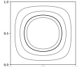
Figure 1: Curves on which the particles are advected by the velocity $\tilde{V}$

We choose to execute the simulation on a regular triangular mesh of size $h\approx\frac{1}{9}$ with $\varepsilon=\frac{1}{100}$. For the time-stepping we use an explicit Runge-Kutta scheme of order 4 with timestep $\Delta t=2^{-16}$ for the DG semi-discretisation and an explicit RK4 with timestep $\frac{\Delta t}{2}$ for the ODE defining the flowmap. In figure 2 we plot the error and the spatial criteria respectively after one and twelve timesteps for the moving mesh and static mesh simulation.

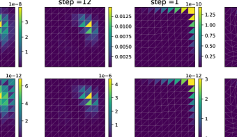
Figure 2: Plot of the criterion (up) and the error (down) after one and after twelve time steps for a static mesh (left) and a moving mesh (right)

In both of these simulations we can see that the error criteria can accurately catch the error. In the static mesh simulation the error is dominated by the advective part, this makes the boundary layer problem less relevant and the refinement would focus on the area where the advection velocity is maximal (black curve in figure 1) and would not resolve smaller scale effects like the boundary layer. In the moving mesh situation we can see that the simulation is more accurate everywhere and in particular in the center of the square and the area with maximal error is on the boundary. Consequently, the mesh refinement would focus on the boundary layer and resolve this small scale effect.

6 Conclusion

In this work we established interior penalty discontinuous Galerkin methods for the semi-discretisation of an Arbitrary Lagrangian-Eulerian formulation in unsteady advection-diffusion problems. By discretising the problem via a dynamically deforming map, we used the existing analytic techniques for advection-diffusion problems with continuous diffusion tensors. This lead us to derive a priori error estimates and made the establishment of a posteriori error criteria possible. The reliability of the a posteriori error estimations were then discussed in a numerical test.

The a priori error estimate shows a condition on the moving mesh velocity for the spatial convergence. This results in a second order convergence in space when the polynomial order is larger than 1, the mesh Peclet number is large and the remaining advection velocity is smaller than the diffusion term. This is a higher order than the one presented in [10].

By focusing on the available data, we derived specific a posteriori criteria for the moving mesh method in two spatial dimensions. The robustness of these error criteria in terms of the mesh Peclet number allowed us to scale the error criteria with the square of the local remaining advection speed (called $\delta$). This behaviour is confirmed by the test cases where the error in terms of the energy-norm appears to strongly depend on this local speed.

In section 5 we showed that this moving mesh method inherits from the robustness properties of the DG method on static meshes. Similarly, the a posteriori error criteria are able to robustly represent the error.

References

• [1] M. Balázsová, M. Feistauer, and M. Vlasák, Stability of the ale space-time discontinuous galerkin method for nonlinear convection-diffusion problems in time-dependent domains†, ESAIM: M2AN, 52 (2018), pp. 2327–2356, https://doi.org/10.1051/m2an/2018062.
• [2] M. Bause and P. Knabner, Uniform error analysis for lagrange–galerkin approximations of convection-dominated problems, SIAM Journal on Numerical Analysis, 39 (2002), pp. 1954–1984, https://doi.org/10.1137/S0036142900367478.
• [3] L. Bonaventura, E. Calzola, and E. e. a. Carlini, Second order fully semi-lagrangian discretizations of advection-diffusion-reaction systems., J Sci Comput, 88 (2021), https://doi.org/10.1007/s10915-021-01518-8.
• [4] E. Burman and P. Zunino, A domain decomposition method based on weighted interior penalties for advection‐diffusion‐reaction problems, SIAM Journal on Numerical Analysis, 44 (2006), pp. 1612–1638, https://doi.org/10.1137/050634736.
• [5] X. Cai, W. Guo, and J. Qiu, Comparison of semi-lagrangian discontinuous galerkin schemes for linear and nonlinear transport simulations, Commun. Appl. Math. Comput., 4 (2020), pp. 3–33, https://doi.org/10.1007/s42967-020-00088-0.
• [6] A. Cangiani, Z. Dong, E. H. Georgoulis, and P. Houston, hp-Version Discontinuous Galerkin Methods on Polygonal and Polyhedral Meshes, Springer Cham, 2017, https://doi.org/10.1007/978-3-319-67673-9.
• [7] A. Cangiani, E. H. Georgoulis, and S. Metcalfe, Adaptive discontinuous galerkin methods for nonstationary convection–diffusion problems, IMA Journal of Numerical Analysis, 34 (2014), pp. 1578–1597, https://doi.org/10.1093/imanum/drt052.
• [8] K. Chrysafinos and N. J. Walkington, Error estimates for the discontinuous galerkin methods for parabolic equations, SIAM Journal on Numerical Analysis, 44 (2006), pp. 349–366, https://doi.org/10.1137/030602289.
• [9] K. Chrysafinos and N. J. Walkington, Lagrangian and moving mesh methods for the convection diffusion equation, ESAIM: M2AN, 42 (2008), pp. 25–55, https://doi.org/10.1051/m2an:2007053.
• [10] V. Dolejší and M. Feistauer, Discontinuous Galerkin Method, Springer Cham, 2015, https://doi.org/10.1007/978-3-319-19267-3.
• [11] A. Ern, A. Stephansen, and P. Zunino, A discontinuous galerkin method with weighted average for advection-diffusion equations with locally small and anisotropic diffusivity, Ima Journal of Numerical Analysis - IMA J NUMER ANAL, 29 (2008), pp. 235–256, https://doi.org/10.1093/imanum/drm050.
• [12] M. Feistauer, J. Hájek, and K. Švadlenka, Space-time discontinuous galerkin method for solving nonstationary convection-diffusion-reaction problems, Appl Math, 52 (2007), p. 197–233, https://doi.org/10.1007/s10492-007-0011-8.
• [13] C. Hirt, A. Amsden, and J. Cook, An arbitrary lagrangian-eulerian computing method for all flow speeds, Journal of Computational Physics, 14 (1974), pp. 227–253, https://doi.org/10.1016/0021-9991(74)90051-5.
• [14] O. A. Karakashian and F. Pascal, A posteriori error estimates for a discontinuous galerkin approximation of second-order elliptic problems, SIAM Journal on Numerical Analysis, 41 (2003), pp. 2374–2399, https://doi.org/10.1137/S0036142902405217.
• [15] C. Klingenberg, G. Schnücke, and Y. Xia, Arbitrary lagrangian-eulerian discontinuous galerkin method for conservation laws: Analysis and application in one dimension, Mathematics of Computation, 86 (2017), pp. 1203–1232, https://doi.org/10.1090/mcom/3126.
• [16] P. H. Lauritzen, R. D. Nair, and P. A. Ullrich, A conservative semi-lagrangian multi-tracer transport scheme (cslam) on the cubed-sphere grid, Journal of Computational Physics, 229 (2010), pp. 1401–1424, https://doi.org/10.1016/j.jcp.2009.10.036.
• [17] M. Restelli, L. Bonaventura, and R. Sacco, A semi-lagrangian discontinuous galerkin method for scalar advection by incompressible flows, Journal of Computational Physics, 216 (2006), pp. 195–215, https://doi.org/10.1016/j.jcp.2005.11.030.
• [18] D. Schötzau and L. Zhu, A robust a-posteriori error estimator for discontinuous galerkin methods for convection–diffusion equations, Applied Numerical Mathematics, 59 (2009), pp. 2236–2255, https://doi.org/10.1016/j.apnum.2008.12.014.
• [19] R. Verfürth, Robust a posteriori error estimators for a singularly perturbed reaction-diffusion equation, Numer. Math., 78 (1998), p. 479–493, https://doi.org/10.1007/s002110050322.
• [20] R. Verfürth, Robust a posteriori error estimates for stationary convection-diffusion equations, SIAM Journal on Numerical Analysis, 43 (2005), pp. 1766–1782, https://doi.org/10.1137/040604261.
• [21] M. F. Wheeler, An elliptic collocation-finite element method with interior penalties, SIAM Journal on Numerical Analysis, 15 (1978), pp. 152–161, https://doi.org/10.1137/0715010.
• [22] L. Zhou, Y. Xia, and C.-W. Shu, Stability analysis and error estimates of arbitrary lagrangian–eulerian discontinuous galerkin method coupled with runge–kutta time-marching for linear conservation laws, ESAIM: M2AN, 53 (2019), pp. 105–144, https://doi.org/10.1051/m2an/2018069.