Strain effects on the electronic properties of a graphene wormhole

Abstract

In this work, we explore the strain and curvature effects on the electronic properties of a curved graphene structure, called the graphene wormhole. The electron dynamics is described by a massless Dirac fermion containing position–dependent Fermi velocity. In addition, the strain produces a pseudo–magnetic vector potential to the geometric coupling. For an isotropic strain tensor, the decoupled components of the spinor field exhibit a supersymmetric (SUSY) potential, depending on the centrifugal term and the external magnetic field only. In the absence of a external magnetic field, the strain yields to an exponential damped amplitude, whereas the curvature leads to a power–law damping of the wave function. The spin–curvature coupling breaks the chiral symmetry between the upper and the lower spinor component, which leads to the increasing of the wave function on either upper or lower region of the wormhole, i.e., depending on the spin number. By adding an uniform magnetic field, the effective potential exhibits an asymptotic quadratic profile and a spin–curvature barrier near the throat. As a result, the bound states (Landau levels) are confined around the wormhole throat showing an asymmetric and spin–dependent profile.

I Introduction

Two dimensional materials, such as graphene geim , silicene silicene and phosphorene phosphorene , have been the subject of intense investigations due to their outstanding properties. Beyond the remarkable mechanical katsnelson and electronic properties Novoselov2004 ; electronic , graphene can also be seen as a table–top laboratory for relativistic physics. Indeed, since the conduction electrons are effectively described as massless Dirac fermions, relativistic effects such as zitterbewegung zitter , Klein tunneling klein and atomic collapse collapse have been observed. Since the graphene layer can assume a curved shape, the curvature effects might lead to new interesting relativistic effects, such as the Hawking–Unruh effect hawking ; hawking2 .

The study of a Dirac fermion confined into a two dimensional surface was initially addressed in Ref.BJ and further developments were provide afterwards diracsurface ; diracsurface2 ; diracsphere . For a relativistic fermion intrinsically living on a curved surface, a physical realization was found for conducting electrons on two dimensional carbon–based structures, as the fullerenes diracintrinsic ; diracintrinsic1 , carbon nanotubes saito and graphitic cones cone . In graphene, the massless Dirac equation in curved spaces was studied in a variety of shapes, such as the localized gaussian bump contijo , the cone furtado , a helical graphene ribbon atanasov ; watanabe , a corrugated plane corrugated , a Möbius ring mobius1 ; mobius2 , a torus ozlem ; Yesiltas:2021crm among others. The surface curvature produces a spin–curvature coupling which leads to a geometric Aharonov–Bohm–like effect geometricphase , a modified spin–orbit coupling geometricsoc ; geometricsoc2 and a geometric spin–Hall effect geometricmonopole .

Besides the curvature, the deformations of the graphene layer modify the effective Dirac fermion dynamics as well, producing the so–called pseudo–magnetic fields ribbons . This vector potential steams from the strain tensor defined by the deformations of the graphene layer and the pseudo–magnetic term comes from the coupling to the Dirac fermion; it is similar to the minimal coupling to a magnetic field gaugestrain . The strain applied to graphene can mimic a strong magnetic field strainstrong and lead to important applications strainappli . From the strain tensor, an effective Hamiltonian for the Dirac fermion was derived using the tight–binding approach vozmediano , containing an anisotropic and position–dependent Fermi velocity and a pseudo–magnetic strain vector in the continuum limit. Since the strain may contain both in–plane and out–of–plane components, the effective Dirac Hamiltonian was extended in order to encompass all the stretching and bending effects vozmediano2 . In addition, the quantum field interaction of the effective Dirac fermion and the strain was discussed in sinner ; gaugegrapheneqft .

An interesting curved graphene structure is the so–called graphene wormhole, where two flat graphene layers are connected by a carbon nanotube wormhole . Since its shape (cylinder) has a non–vanishing mean curvature, the discontinuity of the curvature at the graphene–nanotube junction leads to modifications of the energy spectrum and the possibility of localized states near to it graphenejunction . Although, the Dirac fermions on the upper and lower layers are free states (non–normalizable), the curvature of the nanotube allows the existence of normalizable zero–modes confined at the radius of the wormhole picak ; wormhole3 . In order to avoid the discontinuity at the junction, a smooth graphene wormhole was proposed considering a continuum and asymptotic flat catenoid surface dandoloff ; euclides ; deSouza:2022ioq . The negative curvature of the catenoid leads to a repulsive spin–curvature coupling near the wormhole throat, allowing only the zero–mode as a localized state around the throat wormhole4 ; ozlem2 ; wormhole5 .

In this work, we consider the effects of the curvature and the strain on the effective Dirac fermion living in a catenoid–shaped graphene wormhole. We extend the effective Hamiltonian obtained in vozmediano to a curved surface, introducing the usual spin–connection coupling. We explore the different effects driven by the curvature, isotropic strain and an external magnetic field. Since the surface is asymptotic flat, the lattice deformation which yields the curvature and strain should be concentrated around the throat. The strain leads to a vector potential along the surface meridian, whereas the spin–curvature coupling points in the angular direction. Moreover, the strain vector potential provides an exponential damping of the wave function, whereas the curvature leads to a power–law decay. By adopting the so-called supersymmetric quantum mechanic-like approach ozlem2 , the spinor components exhibit a chiral symmetry breaking. Indeed, the upper component has its probability density enhanced near the wormhole throat in the upper layer, whereas the lower component is enhanced in the lower layer. The ground state zero mode also exhibits this chiral behaviour, since it is exponentially damped either in the upper or in the lower layer depending on the total angular momentum. By applying an uniform magnetic field, the Landau levels are also modified by the curved geometry and strain, leading to asymmetric localized states near the throat.

This work is organized as the follows. In the section (II), we provide a brief review on the catenoid-shape graphene wormhole geometry. In the section (III) we present the effective Hamiltonian containing the strain, curvature and external magnetic field interactions. The section (IV) is devoted to the symmetries of the effective Hamiltonian and in the section (V) we employ the SUSY-QM approach in order to investigate the effects of each interaction. Finally, additional discussion and perspectives are outlined in the section (VI).

II Graphene wormhole geometry

In this section, we define the graphene wormhole surface and describe some of its most important properties. We consider a smooth surface connecting an upper to the lower layer (flat planes). For this purpose, we choose a catenoid shaped surface. In other words, the catenoid surface can be describe in coordinates by euclides ; ozlem2

$$\vec{r}(u,\phi)=\sqrt{R^{2}+u^{2}}\left(\cos\phi\hat{i}+\sin\phi\hat{j}\right)+R\sinh^{-1}\left(\frac{u}{R}\right)\hat{k},$$ (1)

where $R$ is the throat radius, $-\infty<u<\infty$ describes the meridian coordinate and $\varphi$ is the parallel coordinate $\varphi\in[0,2\pi)$, as shown in Fig.1.

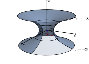
Figure 1: Graphene wormhole geometry. The meridian coordinate $u$ connects the lower to the upper asymptotic flat regions.

The tangent vectors are given by

$$\vec{e}_{1} = \frac{\partial\vec{r}}{\partial u}=\frac{1}{\sqrt{u^{2}+R^{2}}}(u\hat{r}+R\hat{k})$$ (2)

$$\vec{e}_{2} = \frac{\partial\vec{r}}{\partial\phi}=\sqrt{u^{2}+R^{2}}\hat{e}_{2},$$ (3)

where $\hat{e}_{2}=\cos\phi\hat{i}+\sin\phi\hat{j}$ is the unit vector along the $\phi$ direction. From the tangent vectors $(\hat{e}_{1},\hat{e}_{2})$, we can define the surface induced metric $g_{ij}=\vec{e}_{i}\cdot\vec{e}_{j}$. In $(u,\phi)$ coordinates, the surface metric takes the form $g_{ij}=diag(1,(R^{2}+u^{2}))$. Thus, the $2+1$ spacetime interval has the form euclides

$$\mathrm{d}s^{2}=\mathrm{d}t^{2}-\mathrm{d}u^{2}-(R^{2}+u^{2})\mathrm{d}\phi^{2},$$ (4)

where we adopt the $(+,-,-)$ spacetime metric signature convention. Note that the line element in Eq.(4) is invariant under time–translations and rotations with respect to the $\mathrm{z}$ axis (axissymmetric).

Let us now obtain the the main geometric quantities for the electron dynamics, namely, the dreinbeins, connections and curvature. The dreinbeins are related to the spacetime metric by the relation

$$g_{\mu\nu}=e^{a}_{\mu}e^{b}_{\nu}\eta_{ab}.$$ (5)

Thus, for the catenoid, the only non–vanishing components of the dreinbeins are

$$e^{a}_{\mu} = diag(1,1,\sqrt{R^{2}+u^{2}})$$ (6)

Remember that they modify the Fermi velocity by turning it into a position dependet configuration. Moreover, from the dreinbeins, we can defined the moving frame $\theta^{a}=e^{a}_{\mu}\mathrm{d}x^{\mu}$, where, in the catenoid, take the form $\theta^{0}=\mathrm{d}t$, $\theta^{1}=\mathrm{d}u$, $\theta^{2}=\sqrt{R^{2}+u^{2}}\mathrm{d}\phi$. From the torsion–free condition, i.e., $T^{a}=\mathrm{d}\theta^{a}+\omega^{a}_{b}\wedge\theta^{b}=0$, the only non–vanishing one–form connection coefficient $\omega^{a}_{b}=\Gamma_{cb}^{a}\theta^{c}$ is given by

$$\omega^{2}_{1} = \frac{u}{R^{2}+u^{2}}\theta^{2}.$$ (7)

The curvature 2–form $R^{a}_{a}=d\omega^{a}_{b}+\omega^{a}_{c}\wedge\omega^{c}_{b}$ has only non–vanishing component, namely $R^{2}_{1}=-\frac{R^{2}}{(R^{2}+u^{2})^{2}}\theta^{2}\wedge\theta^{1}$. Accordingly, the gaussian curvature $K=\delta^{ab}R_{ab}$ has the form

$$K=-\frac{R^{2}}{(R^{2}+u^{2})^{2}}.$$ (8)

Here, it is important to point out that the catenoid has a negative Gaussian curvature concentrated around the throat and it vanishes in the regions far from it. In Fig. 2, we display the behavior of graphene wormhole curvature $K$. Note that the surface is asymptotically flat. Thus, the effects of the curved geometry and strain on the electron should be concentrated around the origin. Furthermore, as $R\rightarrow 0$, the curvature tends to a $\delta(r)$ function, as it is reported in the literature for a discontinuous graphene wormhole wormhole ; picak ; wormhole3 .

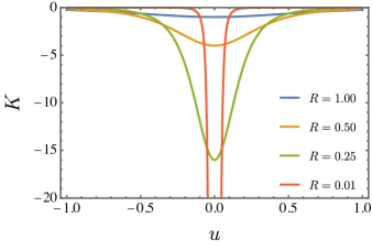
Figure 2: The Gaussian curvature $K(u)$ of the graphene wormhole. The curvature is smooth and concentrated around the throat of the wormhole. For $R\rightarrow 0$, the curvature tends to a delta–like function.

III Strain Hamiltonian

After a brief review of the main geometric properties of the graphene wormhole, let us now discuss the effective Hamiltonian containing the strain and curvature effects on the electron. We follow closely the Ref.(vozmediano ) where the most general effective Hamiltonian was derived. The effective Hamiltonian for a Dirac fermion constrained to a flat surface under influence of the strain and an external magnetic field was found in Ref. (vozmediano ). We propose a generalization of the effective Hamiltonian of Ref.(vozmediano ) in the continuum limit for curved surfaces in the form

$$\mathcal{H}_{D}=-i\hbar\left(v_{i}^{j}\sigma^{i}\partial_{j}+ie\sigma^{i}A_{i}+v_{0}\sigma^{i}\Gamma_{i}+v_{0}\sigma^{i}\Omega_{i}\right),$$ (9)

where $v_{i}^{j}$ is a position–dependent Fermi velocity tensor defined in terms of the strain tensor $u_{ij}$ as vozmediano

$$v_{i}^{j}=v_{0}\left[\delta_{i}^{j}-\frac{\beta}{4}(2u_{i}^{j}+\delta_{i}^{j}u_{k}^{k})\right],$$ (10)

and $v_{0}=\frac{3t_{0}a}{2}$ is the undeformed Fermi velocity, $t$ is the hopping parameter, $a$ is the lattice constant and $\beta=|\partial\ln t/\partial\ln a|$ gaugestrain . The definition of the strain tensor will be given in the next subsection. Note that, when $\beta=0$, the usual constant Fermi velocity is recovered. Besides, the tensor nature of $v_{ij}$ means that the Fermi velocity depends on the direction on the surface.

In addition, the strain on the surface also induces a new vector field, called the strain vector $\Gamma_{i}$, as a divergence of the velocity tensor vozmediano . Thus, for a curved surface, it is defined as

$$\Gamma_{i}=\frac{1}{2v_{0}}\nabla_{j}v^{j}_{i},$$ (11)

where the definition of the strain vector in Eq.(11) is independent of the coordinate choice.

The curved Pauli matrices are defined as watanabe ; mobius1 ; mobius2

$$\sigma^{i}=e^{i}_{a}\sigma^{a},$$ (12)

where $\sigma^{a}$ are the usual flat Pauli matrices, and $e^{i}_{a}$ are the zweinbeins matrices which satisfy

$$g_{ij}=e^{a}_{i}e^{b}_{j}\delta_{ab}.$$ (13)

The definition of the curved sigma matrices employed in Eq.(12) ensures that these matrices do not depend on the particular choice of coordinates of the surface (surface covariance). It is worthwhile to mention that the definitions of the velocity tensor in Eq.(24 and the curved Pauli matrices in Eq.(12) lead to a position and direction dependent Dirac kinetic term $H_{1}=v_{i}^{j}\sigma^{i}\partial_{j}$.

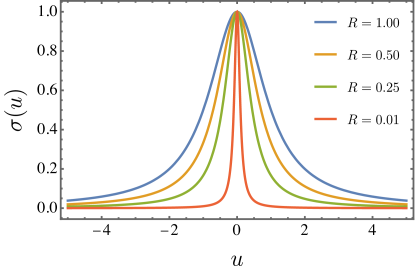
Figure 3: Stress function $\sigma(u)$ for

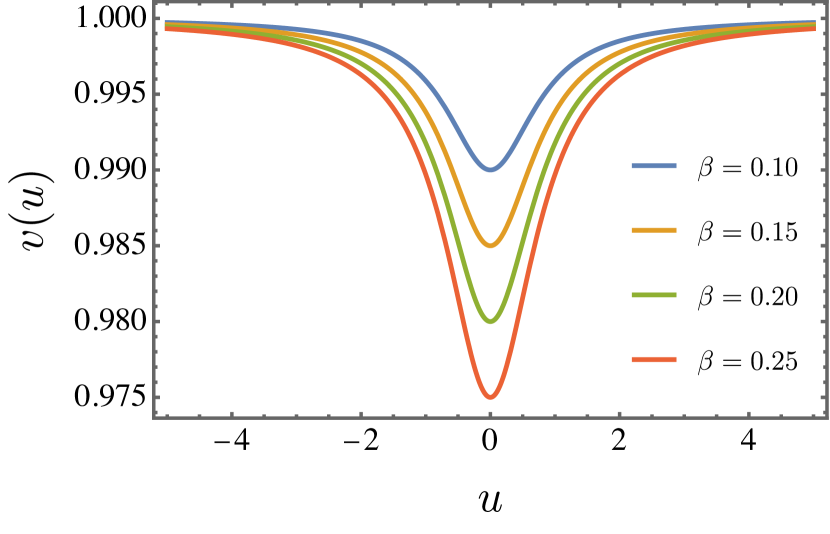
Figure 4: Fermi velocity $v(u)$ for $\beta=0.1$

In the effective Hamiltonian exhibited in Eq.(9), $A_{i}$ is the external magnetic potential and $\Omega_{i}$ is the spinor connection furtado ; mobius2 ; ozlem2

$$\Omega_{i}=\frac{1}{4}\omega_{i}^{ab}\gamma_{a}\gamma_{b}.$$ (14)

The curved $\gamma^{\mu}$ matrices are related to the flat $\gamma^{a}$ ones by the dreinbeins $e^{a}_{\mu}$, i.e., $\gamma^{\mu}=e^{\mu}_{a}\gamma^{a}$. The dreinbeins are defined as $g_{\mu\nu}=e_{\mu}^{a}e_{\nu}^{b}$. In $(2+1)$ dimension, we can adopt the following representation to the flat Dirac $\gamma^{a}$ matrices $\gamma_{0}=\sigma_{3}$, $\gamma_{1}=-i\sigma_{2}$ and $\gamma_{2}=-i\sigma_{1}$ mobius2 ; ozlem ; ozlem2 . Thus, the curved Dirac matrices on the wormhole graphene surface have the form

$$\gamma^{t} = e^{t}_{0}\gamma^{0}=\gamma_{0},$$ (15)

$$\gamma^{u} = \gamma^{1},$$ (16)

$$\gamma^{\phi} = e_{2}^{\phi}\gamma^{2}=\frac{1}{\sqrt{R^{2}+u^{2}}}\gamma^{2}.$$ (17)

From the connection 1–form in Eq.(7), only $\omega^{2}_{1}$ is non zero. Thus, the only non–vanishing component of the spinor connection $\Omega_{\mu}$ is

$$\Omega_{\varphi}=\frac{i}{2}\frac{u}{\sqrt{R^{2}+u^{2}}}\sigma_{3}.$$ (18)

Note that, since $-\infty<u<\infty$, the geometric spinor potential in Eq.(18) is an odd function under parity. This parity violation does not occur for the Dirac fermion in a flat plane diracplanar or the graphitic cone furtado . Moreover, for $R=0$ or for $R\neq 0$ and $u\rightarrow\pm\infty$, the geometric connection is constant, as found for conic surfaces furtado . It is worth mentioning that, due to the resemblance of the spinor and gauge field coupling, the spinor potential is sometimes interpreted as a kind of a pseudo–magnetic potential steaming from the curved geometry contijo .

Furthermore, the strain produces two different potentials on the Dirac electron. The first potential, steaming from the strain in Eq.(11), is a vector potential, whereas the second one in Eq.(18) is a spinorial potential depending on the surface connection. In the next subsections, we choose a particular configuration for the strain and the external magnetic field and explore the differences between these three interactions.

III.1 Strain tensor

Now, let us investigate how the strain tensor $u_{ij}$ modifies the catenoid surface. In order to do it, we assume that the tensions over the surface are static and isotropic. Therefore, we consider the non–uniform isotropic stress tensor in the form

$$\sigma_{j}^{i}=\sigma(u)\delta_{j}^{i}.$$ (19)

Since the catenoid brige is an asymptotically flat surface, we are interested in stress tensor which vanishes away from the throat and it is finite at the origin, i.e.,

$$\lim_{u\rightarrow 0}\sigma(u) = \sigma_{0},$$ (20)

$$\lim_{u\rightarrow\pm\infty}\sigma(u) = 0,$$ (21)

where $\sigma_{0}$ is a constant, which accounts for the maximum value of the surface tension. These conditions guarantee a stress tensor concentrated around the catenoid throat. Indeed, since the surface is asymptotic flat, the curvature and strain effects should vanish as $u\rightarrow\infty$.

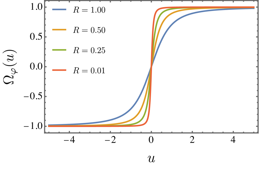
Figure 5: Geometric connection $\Omega_{\phi}$ for $R=0.1$ and $R=1$.

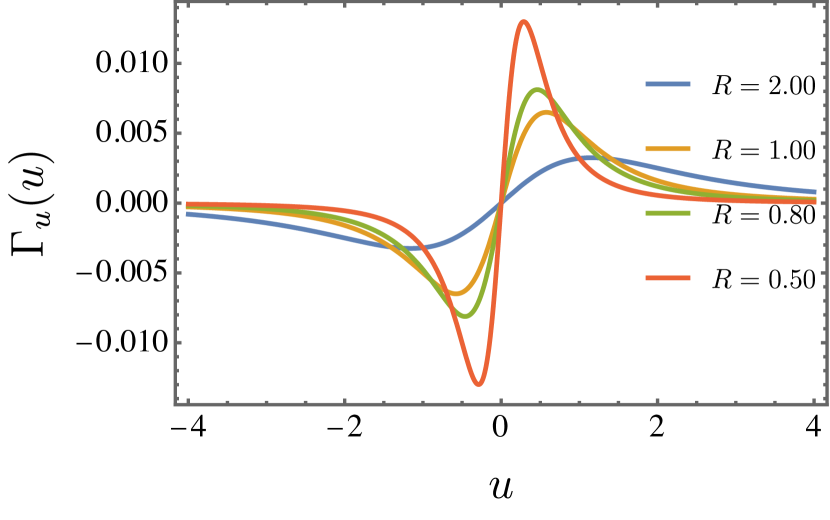
Figure 6: Strain vector $\Gamma_{u}$ for $R=0.1$ and $R=1$.

We assume that the mechanical properties of the surface are in the linear elastic regime. Thereby, the stress and the strain tensors are related by vozmediano

$$\sigma_{ij}=\lambda\theta g_{ij}+2\mu u_{ij},$$ (22)

with $\lambda$ and $\mu$ are the Lamé coefficients and $\theta=u^{i}_{i}$ is the trace of the strain tensor. From the ansatz employed in Eq.(19), we obtain the strain tensor as

$$u^{i}_{j}=\frac{1}{2(\lambda+\mu)}\sigma(u)\delta^{i}_{j}.$$ (23)

The form of the strain tensor in Eq.(23) shows that the deformations undergone by the surface are isotropic and concentrated aroun the catenoid throat. The position–dependent Fermi velocity tensor $v_{ij}$ can be written as

$$v_{i}^{j}=v(u)\delta_{i}^{j},$$ (24)

where the position–dependent Fermi velocity function $v(u)$ is given by

$$v(u)=v_{0}\left[1-\frac{\beta}{2}\frac{\sigma(u)}{\lambda+\mu}\right].$$ (25)

Accordingly, the components of the pseudo–vector potential $\Gamma_{i}$ are

$$\Gamma_{u} = -\frac{\beta}{4}\frac{\sigma^{\prime}(u)}{\lambda+\mu},$$ (26)

$$\Gamma_{\phi} = 0.$$ (27)

In this work, we assume the isotropic stress function $\sigma(u)$ as

$$\sigma(u)=\sigma_{0}\frac{R^{2}}{R^{2}+u^{2}}.$$ (28)

We see that $\sigma(u)$ becomes even more concentrated when $R\rightarrow 0$, as it is shown in Fig. (4). On the other hand, in Fig. (4), we show the plot of the Fermi velocity function $v(u)$ for different values of $\beta$. Remarkably, it decreases for the regions close to the wormhole throat (high curvature). Such a feature was already found in a smooth ripple curved graphene layer contijo .

In addition, the behavior of the geometric spinor connection $\Omega_{\varphi}$ and the strain vector $\Gamma_{u}$ are shown in Fig.(6) and Fig.(6), respectively. Note that both terms are parity odd functions with respect to the $u$ coordinate. In this sense, both potentials yield to barrier between the lower $u<0$ and upper $u>0$ layers. However, despite this similarity, the strain potential given by Eq.(11) and the spinor potential given by Eq.(18) have different natures, forms and components. Therefore, these potentials produce different effects on the Dirac electron, as we shall see in the next section.

III.2 Magnetic vector potential

Now, let us see how the external magnetic field $\vec{B}$ modifies the Hamiltonian. For an uniform magnetic field $\vec{B}=B\hat{k}$, the vector potential $\vec{A}$ is given by $\vec{A}=\frac{1}{2}\vec{B}\times\vec{r}$. Using the coordinates system in Eq.(1), we obtain

$$\vec{A}=\frac{B}{2}\sqrt{R^{2}+u^{2}}\hat{e}_{2}.$$ (29)

For $R=0$, the expression for the vector potential in Eq.(29) reduces to $\vec{A}=\pm\frac{B}{2}u\hat{e}_{2}$, as found in Ref.(diracmagnetic1 ). For $u\gg R$, it yields to $A^{2}\approx\frac{B}{2}u$, as in a conical surface diracmagnetic1 and on the flat plane diracplanar . In addition, at $u=0$, it has a finite value $A^{2}=\frac{BR}{2}$. Since $\vec{e}_{\phi}=\sqrt{R^{2}+u^{2}}\hat{e}_{2}$, the component of $\vec{A}$ in coordinates is given by $A^{\phi}=\frac{B}{2}$. Accordingly, the contravariant component $A_{\phi}=g_{\phi\phi}A^{\phi}$, we have

$$A_{\phi}=\frac{B}{2}(R^{2}+u^{2}).$$ (30)

A similar expression for the vector potential was found for the discontinuous graphene wormhole wormhole3 , except for the presence of the throat radius $R$. The electromagnetic potential displayed in Fig.(10) is parity even, in contrast with the geometric spinor connection shown in Fig.(8). Also, the strain vector in Fig.(8) turns out to have a parity odd configuration.

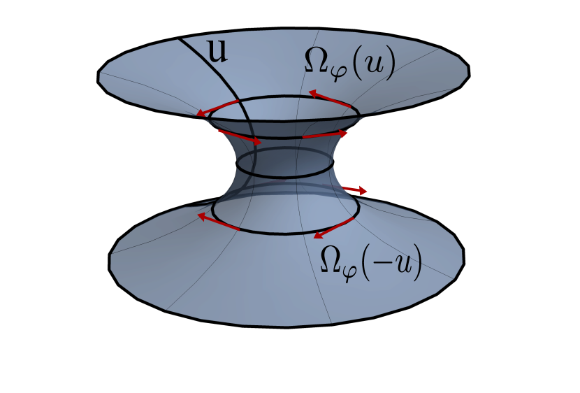
Figure 7: Spin connection $\Omega_{\phi}$ for $R=0.1$ and $R=1$. This curvature potential exhibit a parity–odd angular configuration.

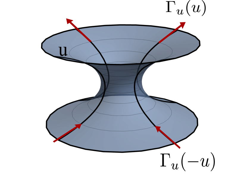
Figure 8: Strain vector $\Gamma_{u}$ for $R=0.1$ and $R=1$. The strain–driven potential has a components only along the meridian.

IV Effective Hamiltonian

Once we have discussed all those interactions acting upon the electron, i.e., the curved geometry, strain and external magnetic field, let us now obtain the respective Hamiltonian. By collecting all the interactions, the effective Hamiltonian becomes

$$\mathcal{H}_{D} = -i\hbar v_{0}\left\{\sigma_{1}\left[v(u)\partial_{u}+\bar{\beta}\sigma^{\prime}+\frac{u}{2(R^{2}+u^{2})}\right]\right.$$ (31)

$$\left.-\frac{i\sigma_{2}}{\sqrt{R^{2}+u^{2}}}[v(u)\partial_{\phi}+eA_{\phi}]\right\},$$

where $\bar{\beta}=\frac{\beta}{4\lambda+\mu}$. Notice that the strain vector and the spinor connection modifies the Dirac equation leading to a canonically momentum on the $u$ of form

$$\hat{P}_{u}=-i\hbar v_{0}\left[v(u)\partial_{u}+\bar{\beta}\sigma^{\prime}+\frac{u}{2(R^{2}+u^{2})}\right].$$ (32)

Additionally, along the angular $\phi$ direction, the canonically conjugate momentum is modified by

$$\hat{P}_{\phi}=-i\hbar v_{0}\frac{1}{\sqrt{R^{2}+u^{2}}}[v(u)\partial_{\phi}].$$ (33)

In this manner, the effective Hamiltonian can be rewritten in the familiar form $\mathcal{H}_{D}=v_{0}\vec{\sigma}\cdot(\vec{P}-e\vec{A}),$ where $\vec{P}=(P_{u},P_{\phi})$ are the canonically conjugate momenta and $\vec{\sigma}=(\sigma_{1},\sigma_{2})$ are the flat Pauli matrices.

The expression in Eq.(31) depends only on the coordinate $u$. The symmetry of the Hamiltonian with respect to the angular $\phi$ variable is the result of the surface axial symmetry. Thus, the wave function should also inherit this symmetry. In fact, consider the angular momentum operator with respect to the $\mathrm{z}$ axis, $\hat{L}_{z}=-i\hbar\frac{\partial}{\partial\phi}$ such that, $\hat{L}_{z}\psi=\hbar l\psi$, where $l$ is the orbital angular momentum with respect to the $\mathrm{z}$ axis. For a non–relativistic and spinless electron on the graphene wormhole, an axissymmetric wave function can be written as $\psi(u,\phi)=e^{il\phi}\psi(u)$ euclides . However, as it is well–known for the relativistic electron, $\hat{L}_{z}$ no longer commute with $\mathcal{H}_{D}$, although the total angular momentum operator along the $z$ direction $\hat{J}_{z}=\hat{L}_{z}+\hat{S}_{z}$ does diracplanar . Since $\hat{S}_{3}=\frac{\hbar}{4}[\gamma^{1},\gamma^{2}]$, then the spin operator with respect to the $\mathrm{z}$ axis is given by

$$S_{z}=-i\frac{\hbar}{2}\sigma_{3}.$$ (34)

Here, the total angular momentum operator has the form $\hat{J}_{z}=-i\hbar\left(\frac{\partial}{\partial\phi}+\frac{1}{2}\sigma_{3}\right)$, where $\hat{J}\psi=m\hbar\psi$ and $m=l\pm 1/2$ diracplanar2 . Therefore, considering the axial symmetry on the spinorial wave function, so that wormhole4 ; diracplanar2

$$\Psi(u,\phi)=e^{im\phi}\psi(u),$$ (35)

the Dirac equation $\mathcal{H}_{D}\Psi=E\Psi$ leads to the Dirac equation $\tilde{\mathcal{H}}_{D}\psi=E\psi$, in which the effective Hamiltonian simplifies to

$$\tilde{\mathcal{H}}_{D} = -i\hbar v_{0}\left(\begin{array}[]{cc}0&v(u)\partial_{u}+\bar{\beta}\sigma^{\prime}+\frac{u}{2(R^{2}+u^{2})}-\frac{[v(u)m+eA_{\phi}]}{\sqrt{R^{2}+u^{2}}}\\ v(u)\partial_{u}+\bar{\beta}\sigma^{\prime}+\frac{u}{2(R^{2}+u^{2})}+\frac{[v(u)m+eA_{\phi}]}{\sqrt{R^{2}+u^{2}}}&0\end{array}\right).$$ (38)

Since the effective Hamiltonian in Eq.(38) has parity violating terms steaming from the geometric connection and the strain vector, we can not assume that the spinor $\psi=\left(\begin{array}[]{cc}\psi_{1}\\ \psi_{2},\end{array}\right)$ is parity invariant. This parity violation of the Dirac spinor on the graphene wormhole is in contrast with the relativistic electron on a flat plane diracplanar ; diracplanar2 .

In Eq.(38), the position–dependent velocity function $v(u)$ multiplies the partial derivative $\partial_{u}$. By writing $v\frac{d}{du}=\frac{d}{d\zeta}$, for $v(u)$ given by Eq.(25), we have $\zeta=u-\bar{\beta}R\,\tanh^{-1}\left(\frac{\sqrt{u}u}{\sqrt{\bar{\beta}-2}R}\right)$. Unfortunately, this relation analytically can not be inverted, seeking to rewrite Eq. (38) in terms of variable $\zeta$. Nevertheless, a graphic analysis reveals only a small difference between $\zeta$ and $u$ as shown in Fig. 12. Analogously, for the sake of simplicity, we adopt $\zeta\approx u$ from now on.

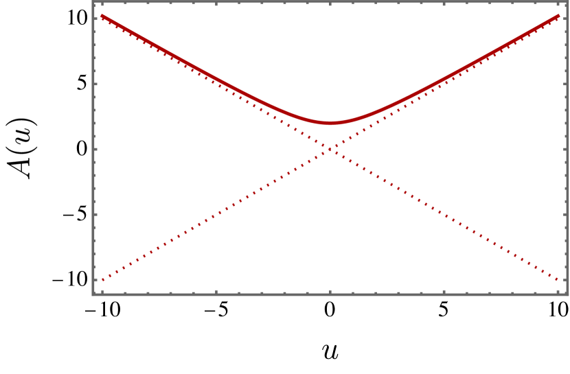
Figure 9: Vector potential angular component for an uniform magnetic field.

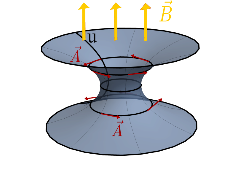
Figure 10: Magnetic vector potential $\vec{A}$ on the surface.

As a result, the Hamiltonian simplifies to

$$\tilde{\mathcal{H}}_{D} = -i\hbar v_{0}\left(\begin{array}[]{cc}0&\partial_{u}+\bar{\beta}\sigma^{\prime}+\frac{u}{2(R^{2}+u^{2})}-\frac{[m+eA_{\phi}]}{\sqrt{R^{2}+u^{2}}}\\ \partial_{u}+\bar{\beta}\sigma^{\prime}+\frac{u}{2(R^{2}+u^{2})}+\frac{[m+eA_{\phi}]}{\sqrt{R^{2}+u^{2}}}&0\end{array}\right).$$ (41)

The effective Hamiltonian in Eq.(41) shows clearly the distinctive interaction terms steaming from the strain $\bar{\beta}\sigma^{\prime}$, from the geometric connection $\frac{u}{2(R^{2}+u^{2})}$, centrifugal term $\frac{m}{\sqrt{R^{2}+u^{2}}}$ and the electromagnetic coupling $\frac{eA_{\phi}}{\sqrt{R^{2}+u^{2}}}$. In the next section, we explore the effects of each interaction.

V Supersymmetric analysis

In this section, we employ a supersymmetric quantum mechanical approach ozlem ; ozlem2 to explore the features of the effective Hamiltonian in Eq.(41) and find the solutions of the Dirac equation.

From the effective Eq.(41), it leads to

$$\tilde{\mathcal{H}}_{D}\psi=\epsilon\psi,$$ (42)

where the spinor $\psi=\left(\begin{array}[]{cc}\psi_{1}\\ \psi_{2},\end{array}\right)$. The effective Dirac equation (42) can be written as

$$\left(\begin{array}[]{cc}0&i\mathcal{O}_{2}\\ i\mathcal{O}_{1}&0\end{array}\right)\left(\begin{array}[]{cc}\psi_{1}\\ \psi_{2},\end{array}\right)=\epsilon\left(\begin{array}[]{cc}\psi_{1}\\ \psi_{2},\end{array}\right),$$ (49)

where the firs–order operators $\mathcal{O}_{1,2}$ are defined as

$$\mathcal{O}_{1,2}=\frac{\mathrm{d}}{\mathrm{d}u}+\bar{\beta}\sigma^{\prime}+\frac{u}{2(R^{2}+u^{2})}\pm\frac{(m+eA_{\phi})}{\sqrt{R^{2}+u^{2}}}.$$ (50)

By performing the change on the wave function of the form

$$\psi_{1,2}(u)=(R^{2}+u^{2})^{-1/4}e^{-\bar{\beta}\sigma(u)}\chi_{1,2}(u),$$ (51)

the Dirac equation yields to a decoupled equations for the $\chi_{1}$ and $\chi_{2}$ in a Klein–Gordon like form

$$-\chi_{1,2}^{\prime\prime}+U_{eff1,2}^{2}\chi_{1,2}=\epsilon^{2}\chi_{1,2},$$ (52)

where $\epsilon=\frac{E}{\hbar v_{0}}$ is the electron momentum and the effective squared potential is given by

$$U_{eff1,2}^{2}=\left(\frac{(m+eA_{\phi})}{\sqrt{R^{2}+u^{2}}}\right)^{2}\mp\left(\frac{(m+eA_{\phi})}{\sqrt{R^{2}+u^{2}}}\right)^{\prime}.$$ (53)

The Klein–Gordon–like expression present in Eq. (52) has the structure of a so–called supersymmetric quantum mechanics, whose superpotential $W$ is given by

$$W=\frac{m+eA_{\phi}}{\sqrt{R^{2}+u^{2}}}.$$ (54)

Note that Eq.(54) is given by the spin–curvature potential $\frac{m}{\sqrt{R^{2}+u^{2}}}$ and the magnetic coupling term $\frac{eA_{\phi}}{\sqrt{R^{2}+u^{2}}}$ present in the Dirac equation.

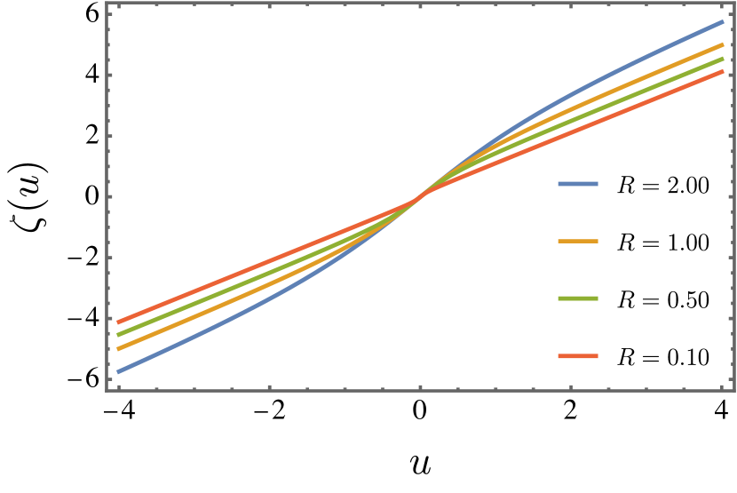
Figure 11: Change of coordinate $\zeta=\zeta(u)$ for $\beta=1$.

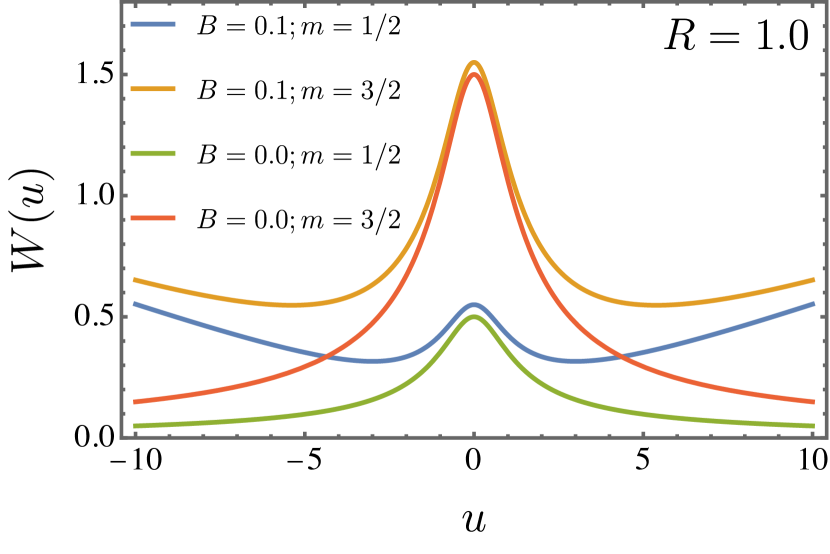
Figure 12: Superpotential $W(u)$ for $R=1$, $B=0$.

The SUSY–like form of the effective squared potential

$$U_{eff1,2}^{2}=W^{2}\mp W^{\prime}$$ (55)

enables us to rewrite the decoupled system of second–order Klein–Gordon like Eq.(52) as

$$a^{\dagger}a\chi_{1}=\epsilon^{2}\chi_{1}$$ (56)

$$aa^{\dagger}\chi_{2}=\epsilon^{2}\chi_{2},$$ (57)

where $a=\frac{d}{du}+W$ and $a^{\dagger}=-\frac{d}{du}+W$ are first–order differential operators ozlem2 . The so-called superpartner squared-Hamiltonians $H_{1}^{2}=a^{\dagger}a$ and $H_{2}^{2}=aa^{\dagger}$ satisfy $H_{2}^{2}=(H_{1}^{2})^{\dagger}$ ozlem2 .

A remarkable feature of a quantum mechanical SUSY–like eq.(56) is the existence of a nonvanishing ground state for $\epsilon=0$, known as the zero mode wormhole ; picak . Indeed, for $\epsilon=0$, the conditions $a\chi_{1}=0$ and $a^{\dagger}\chi_{2}$ yield to

$$\psi^{0}_{1,2}(u)=(R^{2}+u^{2})^{-1/4}e^{-\bar{\beta}\sigma(u)}e^{\mp\int{W(u^{\prime})du^{\prime}}}.$$ (58)

Since the superpotential $W$ is related to the spin–curvature coupling and the external magnetic field, the zero mode is related to the flux of curvature and magnetic field near the throat wormhole .

The factor $(R^{2}+u^{2})^{-1/4}$ steams from the normalization condition on the surface. Indeed, the normalization constant takes the form

$$1=\int_{-b}^{b}\int_{0}^{2\pi}{||\psi||^{2}(R^{2}+u^{2})^{1/2}\mathrm{d}u\mathrm{d}\phi},$$ (59)

where $-b<u<b$. Despite both the curved geometry and the strain reduce the wave function amplitude for $u\rightarrow\pm\infty$, the curvature damps the amplitude by a potential factor whereas the strain damps it by an exponential factor.

Another noteworthy feature of the Dirac equation in curved surface is related to the geometric phase furtado . Indeed, the holonomy operator $U(\phi)=e^{\int_{0}^{\phi}{\Omega_{i}dx^{i}}}$, where $\Omega_{i}$ is the spin connection in Eq.(18) leads to

$$U(\phi)=e^{-\frac{i}{2}\frac{u}{R^{2}+u^{2}}\sigma_{3}\phi}.$$ (60)

This geometric phase reflects the change on the wave function when the fermion performs a $2\pi$ rotation for a given $u$ mobius2 . It is a kind of geometric Aharonov–Bohm effect driven by the curvature instead of the magnetic field furtado . By applying the geometric phase operator $U(\phi)$, i.e., $\psi^{\prime}=U(\phi)\psi$, the Dirac equation $\tilde{\mathcal{H}}_{D}\psi=E\psi$ simplifies to $\hat{\mathcal{H}}_{D}\psi^{\prime}=E\psi^{\prime}$, where the simplified Hamiltonian $\hat{\mathcal{H}}_{D}$ is given by

$$\tilde{\mathcal{H}}_{D} = -i\hbar v_{0}\left(\begin{array}[]{cc}0&\partial_{u}+\bar{\beta}\sigma^{\prime}-\frac{[m+eA_{\phi}]}{\sqrt{R^{2}+u^{2}}}\\ \partial_{u}+\bar{\beta}\sigma^{\prime}+\frac{[m+eA_{\phi}]}{\sqrt{R^{2}+u^{2}}}&0\end{array}\right).$$ (63)

Thus, the curvature effects of the curved surface can be encoded into the geometric phase in the operator $U(\phi)$ given by Eq.(60).

It is important to highlight that the effects of the strain, curved geometry and the external magnetic fields are rather distinct. The strain and curved geometry provide the geometric phase, whereas the centrifugal and the magnetic field yield to the SUSY–like symmetry. In the following, we explore the effects of the each term on the electronic states.

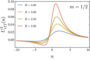
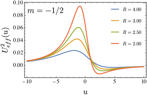
Figure 13: Effective squared potential for $m=1/2$ (on the left panel), $m=-1/2$ (on the right panel) for $B=0$.

V.1 No external magnetic field

In the absence of a magnetic field, i.e., for $B=0$, the superpotential has a simple form

$$W(u)=\frac{m}{\sqrt{R^{2}+u^{2}}},$$ (64)

whose behavior is plotted in Fig.12. The symmetric centrifugal barrier of the superpotential yields to an asymmetric potential for $U^{2}_{eff}$, as shown in Fig. 13. Note the dependence of the squared potential on the total angular momentum $m$. This one is similar to that one encountered in the context of a Dirac electron constrained to a helicoid potential watanabe .

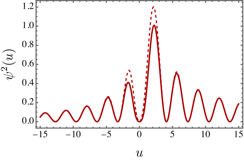
Figure 14: Density of states for $\epsilon=1$ and $m=1/2$.

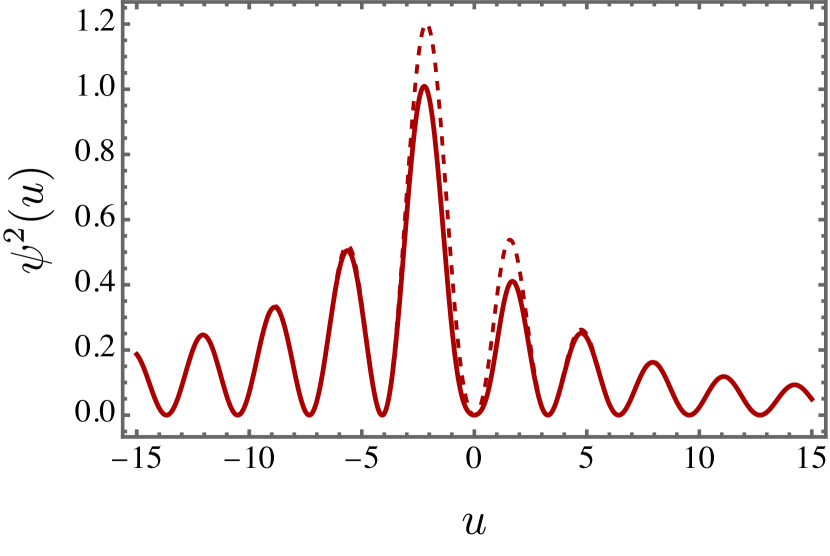
Figure 15: Density of states for $\epsilon=1$ and $m=-1/2$.

For $m\neq 0$, the Klein–Gordon like eq.(52) reads

$$-\chi_{1,2}^{\prime\prime}+\left(\frac{m^{2}}{R^{2}+u^{2}}\pm m\frac{u}{(R^{2}+u^{2})^{3/2}}\right)\chi_{1,2}=\epsilon^{2}\chi_{1,2},$$ (65)

It is worthwhile to mention that the effective potential

$$U^{2}_{eff1,2}=\frac{m^{2}}{R^{2}+u^{2}}\pm m\frac{u}{(R^{2}+u^{2})^{3/2}},$$ (66)

couples the angular momentum quantum number $m$ and the curved geometry terms. The second term in the potential $\frac{m}{(R^{2}+u^{2})^{3/2}}$ breaks the symmetry $m\rightarrow-m$. Indeed, we can obtain the $\chi_{2}$ spinor component from $\chi_{1}$ by performing the change $m\rightarrow-m$.

For $u>>R$, the potential tends to $U_{eff1,2}\approx\frac{m(m\pm 1)}{u^{2}}$. Accordingly, the Eq.(65) has the asymptotic solution

$$\chi_{1,2}\approx\sqrt{u}\left(c_{1}J_{\frac{2m\pm 1}{2}}(\epsilon u)+c_{2}Y_{\frac{2m\pm 1}{2}}(\epsilon u)\right),$$ (67)

where $J_{n}(x)$ and $Y_{n}(x)$ are the Bessel function of the first kind and the second kind, respectively. In this region, the solution in Eq.(67) resembles the one found for the Dirac equation in other graphene wormhole geometries outside the throat wormhole4 .

Note the presence of the total angular momentum number $m=l+\frac{1}{2}$ in the order of the Bessel functions. For $u\rightarrow\pm\infty$, the potential vanishes and thus, the $\chi_{1}$ function tends to $A\sin(\epsilon u)$, as for the $m=0$ states. Therefore, the interaction between angular momentum and curvature is concentrated around the graphene wormhole throat.

For $R=1$ and $\epsilon=1$, we numerically solved the Eq.(65) and the resulting squared wave function was plotted in fig.(15) for $m=1$ and in the fig.(15) for $m=-1$. By changing $m\rightarrow-m$, the density of state is shift from the upper $(u>0)$ into the lower sheet $(u<0)$. Moreover, for $\beta=1$ (thick line) the amplitude is smaller than for $\beta=0.5$ (dashed line).

The zero mode, i.e., for $\epsilon=0$ is given by

$$\psi^{0}_{1,2}(u)=(R^{2}+u^{2})^{-1/4}e^{-\bar{\beta}\sigma(u)}e^{\mp m\sinh^{-1}(u/R)},$$ (68)

where is evident the chiral symmetry breaking $m\rightarrow-m$ and the parity-odd behaviour of this ground state. Indeed, as shown in the fig. the states for $m>0$ are suppressed in the upper layer whereas the $m<0$ states are suppressed in the lower layer. A similar chiral separation was also found for the massless Dirac field in a helicoidal graphene strip atanasov .

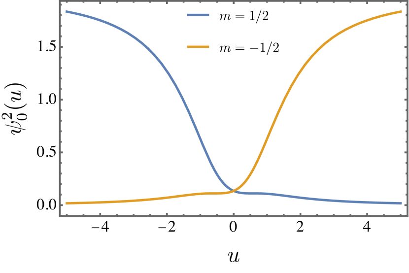
Figure 16: Zero mode for $m=\pm 1/2$.

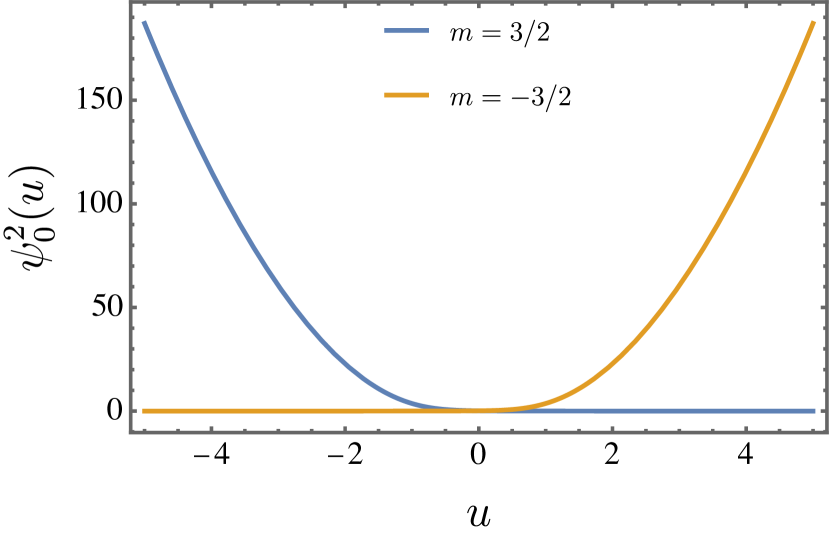
Figure 17: Zero mode $m=\pm 3/2$.

V.2 Constant magnetic field

Now let us consider the additional effects from the uniform magnetic field. The respective Klein-Gordon like equation becomes

$$-\chi_{1,2}^{\prime\prime}+\left(\frac{(m+(Bu^{2})/2)^{2}}{R^{2}+u^{2}}\mp\frac{u(-2m+B(2R^{2}+u^{2}))}{2(R^{2}+u^{2})^{3/2}}\right)\chi_{1,2}=\epsilon^{2}\chi_{1,2}.$$ (69)

In the eq.(69), the effective potential

$$U^{2}_{eff1,2}=\frac{(m+(Bu^{2})/2)^{2}}{R^{2}+u^{2}}\mp\frac{u(-2m+B(2R^{2}+u^{2}))}{2(R^{2}+u^{2})^{3/2}}$$ (70)

includes effects from the curved geometry, total angular momentum (spin and orbital), and the coupling to the magnetic field. Note that, for $u\gg R$ (outside the throat), the effective potential takes the form

$$U^{2}_{eff}\approx\frac{m(m+1)}{u^{2}}+B\left(m-\frac{1}{2}\right)+\frac{B^{2}}{4}u^{2},$$ (71)

which is the effective potential for a $2+1$ massless Dirac fermion under an uniform magnetic field in a flat plane using cylindrical coordinates diracplanar ; diracplanar2 . That is an expected result, since the graphene wormhole surface is asymptotic flat. Moreover, the effective potential in Eq.(70) also exhibits the $m\rightarrow-m$ asymmetry.

Due to the complexity of eq.(69) we employ numerical methods to obtain the first excited states and their respective energy spectrum (Landau levels). In the figures (19) and (19) we plotted the effective potential $U^{2}_{eff}$ for $m=0$ and $m=1$, respectively. Note that for $u\gg R$, the effective potential diverges as $\frac{B^{2}}{4}u^{2}$, whereas for $u\ll R$ the potential is dominated by the geometric and angular momentum terms (finite barrier for $m\neq 0$).

We plotted the first Landau levels for $eB=1$, $R=1$, $\beta=1$ and $m=0$ (s state) in the fig.(21. Note that the first excited state (red line) is located on the upper layer, whereas the second (blue) and the third (green) have two asymmetric peaks around the origin. For $eB=1$, $R=1$, $\beta=1$ and $m=2$ in the fig.(21), the first excited state already has two asymmetric peaks displaced from the origin. Nonetheless, it is worthwhile to mention that the probability density does not vanishes at the origin. Note that for $u\gg R$, the wave function exhibits the usual exponential decay due to the external magnetic field diracplanar . Therefore, the external magnetic field allow us to confine the electron around the wormhole throat. However, due to the curved geometry and the strain, the electron is not symmetric confined around the wormhole.

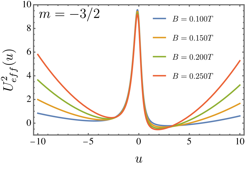
Figure 18: Effective squared potential for $m=-3/2$ for different values of $B$.

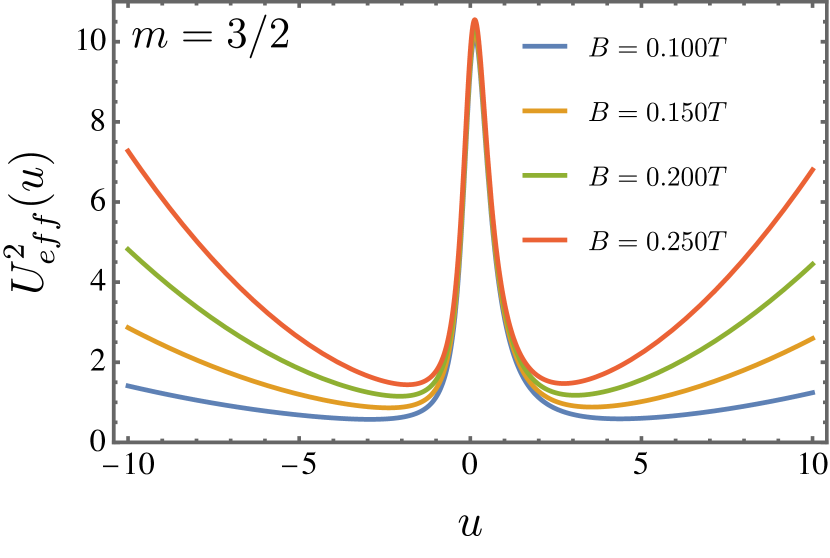
Figure 19: Effective squared potential for $m=3/2$. Red line(B=0.1), blue line (B=0.15) and the green line (B=0.2).

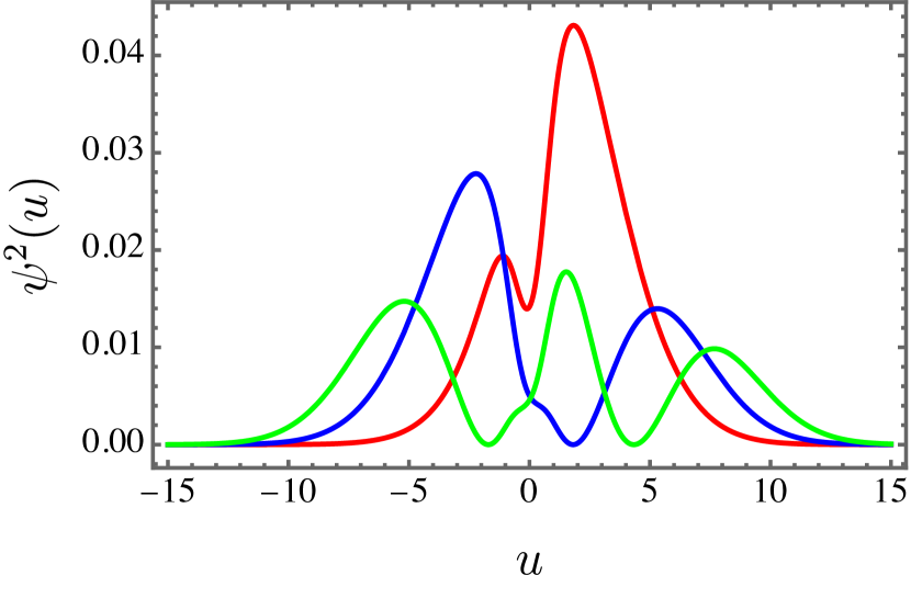
Figure 20: Density of states for $B=0.1$ and $m=1/2$. The ground state (red line) has a peak in the upper layer whereas the first excited state (blue line) is more localized in the lower layer. The second excited state exhibits three less distinct peaks.

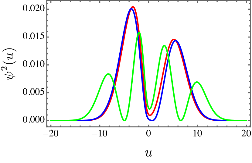
Figure 21: Density of states for $B=0.1$ and $m=3/2$.The ground state (red line) has a peak in the upper layer whereas the first excited state (blue line) is more localized in the lower layer. The second excited state exhibits three less distinct peaks.

Finally, the ground state zero mode under the action of the magnetic field is modified by

$$\psi^{0}_{1,2}(u) = (R^{2}+u^{2})^{-1/4}e^{-\bar{\beta}\sigma(u)}e^{\mp m\sinh^{-1}(u/R)}$$ (72)

$$\times e^{\mp\frac{eB}{4}(u\sqrt{R^{2}+u^{2}}+R^{2}\tanh^{-1}(u/\sqrt{R^{2}+u^{2}}))}.$$

In the eq.(72), the magnetic field introduces another exponential factor whose argument is a parity-odd function. Accordingly, the magnetic field enhances the chiral separation of the eletronic modes. However, note that shifting the sign of the magnetic field for a given angular momentum number $m$, the magnetic field might reduce the chiral separation between the upper and lower layers.

VI Final remarks and perspectives

We investigated the curvature, strain and magnetic field effects upon a massless relativistic electron on a graphene wormhole surface. The graphene wormhole was described by a catenoid surface which smoothly connects two asymptotic flat graphene planes (layers). In this sense, the geometry proposed was a smooth generalization of the graphene wormhole shown in the Ref.wormhole . The effective Dirac Hamiltonian containing strain–dependent terms was obtained in Ref.vozmediano and extended in Ref.vozmediano2 .

Due to the axial symmetry, we considered an isotropic strain tensor localized near the wormhole throat, similar to the behavior of the Gaussian curvature. Indeed, since the curved geometry of the throat was obtained due to deformation of the lattice structure, it was expected that both curvature and strain were localized around this region. It turned out that the pseudo–magnetic potential due to the strain $\Gamma_{u}$ had only components along the meridian coordinate $u$, whereas the spin connection $\Omega_{\phi}$ pointed along the parallel direction $\phi$. In this manner, despite of having the same origin (the lattice deformation), these two interactions had distinct effects on the electron. Moreover, by applying the external magnetic field, a true magnetic potential $\vec{A}$ also acted on the electron. Nevertheless, although $\vec{A}$ only had the angular component $A_{\phi}$, the spin connection $\Omega_{\phi}$ was parity–odd, whereas $A_{\phi}$ was parity–even under the transformation $u\rightarrow-u$.

The strain and spin–curvature brook the parity invariance of the effective Hamiltonian. Moreover, the spin–connection term led to a chiral invariance $m\rightarrow-m$. By employing the supersymmetric quantum mechanichal (QMSUSY) approach, we found that the strain vector yielded to an exponential suppression of the wave function, whereas the spin connection led to a power–law decay. In absence of magnetic field, the superpotential was given by the spin–curvature term which increased the amplitude of the probability density in the upper layer for $m>0$ and in the lower layer for $m<0$. A similar chiral behavior was found in graphene nanoribbons in a helical shape atanasov . Since the graphene structure is asymptotically flat, for a vanishing strain vector, the wave function behaves as a free wave in a flat plane watanabe . The inclusion of an uniform magnetic field confined the electronic states near the wormhole throat. These Landau levels were modified by the spin–curvature and the strain interactions turned out to be an asymmetric probability distribution.

In addition, this work revealed that, in spite of the coupling of strain, curvature and magnetic field in the effective Dirac Hamiltonian were similar, they possessed rather different effects. As a result, we pointed out a couple of perspectives for further investigations. A noteworthy extension of the present work could be considering the effects of a a dynamical strain (phonons) or corrugations on the graphene wormhole. Furthermore, the chiral breaking due to the spin–curvature coupling suggests an interesting spin–Hall current to be analysed. Moreover, the analysis of the geometric Aharonov–Bohm like phase due to the concentrated curvature around the wormhole throat seems a worthy perspective as well.

References

- (1) A. K. Geim, Science, v. 324, (2009) 1530.
- (2) A. Kara et al, Surf. Sci. Rep. 67, 1, (2012).
- (3) A. Carvalho, M. Wang, X. Zhu, A. S. Rodin, H. Su, A. H. Castro Neto, Nat. Rev. Mat. 1, 11 (2016).
- (4) M. I. Katsnelson, Graphene: carbon in two dimensions, Cambridge University Press (2012).
- (5) K. S. Novoselov, K. Geim, V. Morozov, D. Jiangy, Y. Zhangs, S. V. Dubonos, V. Grigorieva and A. A. Firsov, Science 306, (2004) 666.
- (6) A. H. Castro Neto, F. Guinea, N. M. R. Peres, K. S. Novoselov, and A. K. Geim, Rev. Mod. Phys. 81, 109 (2009).
- (7) M. I. Katsnelson, Eur. Phys. J. B 51, 157–160 (2006).
- (8) M. I. Katsnelson, K. S. Novoselov, A. K. Geim, Nature Physics volume 2, 620 (2006).
- (9) A. V. Shytov, M. I. Katsnelson, L. S. Levitov, Phys. Rev. Let. 99, (2007).
- (10) A. Iorio, G. Lambiase, Phys. Lett. B 716, 334 (2012).
- (11) T. Morresi et al, 2D Mater. 7, 041006 (2020).
- (12) M. Burgess, B. Jensen, Phys. Rev. A 48, 3, 1861 (1993).
- (13) F.T. Brandt, J.A. Sanchez-Monroy, Phys. Let. A 380, 38, 3036 (2016).
- (14) H. Zhao, Y. L. Wang, C.Z. Ye, R. C., G. H. Liang, and H. Liu Phys. Rev. A 105, 052220 (2022).
- (15) Q. H. Liu, Z. Li, X. Y. Zhou, Z. Q. Yang, W. K. Du Eur. Phys. J. C 79, 712 (2019).
- (16) J. González, F. Guinea, M.A.H. Vozmediano, Phys. Rev. Lett. 69, 172 (1992).
- (17) J. González, F. Guinea, M.A.H. Vozmediano, Nuclear Physics B, (1993).
- (18) Saito R., Dresselhaus G. and Dresselhaus M. S., Physical Properties of Carbon Nanotubes, I. C. Press, London 1998.
- (19) P. Lammert and V. Crespi, Phys. Rev. lett. 85, 5190 (2000).
- (20) F. de Juan, A. Cortijo, M. A. H. Vozmediano, Phys. Rev. B 76, 165409, (2007).
- (21) C. Furtado , F. Moraes , A.M. de M. Carvalho, Phys. Lett. A 372, 5368, (2008).
- (22) V. Atanasov, A. Saxena, Phys. Rev. B 92, 035440 (2015).
- (23) M. Watanabe, H. Komatsu, N. Tsuji, and H. Aoki Phys. Rev. B 92, 205425 (2015).
- (24) V. Atanasov, A. Saxena, Phys. Rev. B 81, 205409 (2010).
- (25) K. Flouris, M. M. Jimenez, and H. J. Herrmann, Phys. Rev. B 105, (2022) 235122.
- (26) L. N. Monteiro, C. A. S. Almeida, and J. E. G. Silva Phys. Rev. B 108, 115436 (2023).
- (27) Ö. Yeşiltaş Advances in high energy physics, 6891402 (2018).
- (28) Ö. Yeşiltaş and J. Furtado, Int. J. Mod. Phys. A 37 (2022) no.11n12, 2250073
- (29) F. de Juan, A. Cortijo, María A. H. Vozmediano, A. Cano, Nature Physics 7, 810 (2011).
- (30) A. Shitade and E. Minamitani, New J. Phys. 22, 113023 (2020).
- (31) G. Liang, Y. Wang, M. Lai, H. Liu, H. Zong and S. Zhu Phys. Rev. A 98, 062112 (2018).
- (32) Y. Wang, H. Zhao, H. Jiang, H. Liu and Y. Chen Phys. Rev. B 106, 235403, (2022).
- (33) F. Guinea, A. K. Geim, M. I. Katsnelson, and K. S. Novoselov, Phys. Rev. B 81, 035408 (2010).
- (34) M.A.H. Vozmedianoa, M.I. Katsnelson, F. Guinea, Phys. Rep. 496, 109 (2010).
- (35) Levy, N. et al., Science 329, 544–547 (2010).
- (36) Guinea, F., Katsnelson, M. I. and Geim, A. K., Nature Phys. 6, 30–33 (2010).
- (37) F. de Juan, J. L. Mañes, and M. A. H. Vozmediano Phys. Rev. B 87, 165131 (2013).
- (38) J. L. Mañes, F. de Juan, M. Sturla, and M. A. H. Vozmediano, Phys. Rev. B 88, 155405 (2013).
- (39) A. Sinner and K. Ziegler, Ann. Phys. 400, 262-278 (2019).
- (40) E. Arias, A. R. Hernandez and C. Lewenkopf, Phys. Rev. B 92, 245110 (2015).
- (41) J. González, J. Herrero, Nucl. Phys. B 825, 426 (2010).
- (42) J. Gonzalez, F. Guinea, J. Herrero, Phys. Rev. B 79, 165434 (2009).
- (43) R. Pincak, J. Smotlacha, Quantum Matter 5, 114 (2016).
- (44) G.Q. Garcia, P.J. Porfírio, D.C. Moreira and C. Furtado, Nucl. Phys. B 950, 114853 (2020).
- (45) R. Dandoloff, A. Saxena, B. Jensen, Phys. Rev. A 81, 014102 (2010).
- (46) J.E.G. Silva et al., Phys. Lett. A 384, 126458 (2020).
- (47) T. F. de Souza, A. C. A. Ramos, R. N. Costa Filho and J. Furtado, Phys. Rev. B 106 (2022) no.16, 165426
- (48) K. Pimsamarn, P. Burikham, T. Rojjanason, Eur. Phys. J. C 80, 1111 (2020).
- (49) Ö. Yeşiltaş, J. Furtado, and J. E. G. Silva, Eur. Phys. J. Plus, 137, (2022) 416.
- (50) E. Cavalcante, Eur. Phys. J. Plus 137, 1351 (2022).
- (51) C. Ho and V. R. Khalilov, Phys. Rev. A 61, 032104 (2000).
- (52) V.M. Villalba and A. R. Maggiolo, Eur. Phys. J. B 22, 31–35 (2001).
- (53) M. J. Bueno, C. Furtado and A. M. de M. Carvalho, Eur. J. Phys. B 85, 53 (2012).