Analysis of the Geometric Structure of Neural Networks and Neural ODEs via Morse Functions

Abstract

Besides classical feed-forward neural networks, also neural ordinary differential equations (neural ODEs) gained particular interest in recent years. Neural ODEs can be interpreted as an infinite depth limit of feed-forward or residual neural networks. We study the input-output dynamics of finite and infinite depth neural networks with scalar output. In the finite depth case, the input is a state associated to a finite number of nodes, which maps under multiple non-linear transformations to the state of one output node. In analogy, a neural ODE maps a linear transformation of the input to a linear transformation of its time-$T$ map. We show that depending on the specific structure of the network, the input-output map has different properties regarding the existence and regularity of critical points. These properties can be characterized via Morse functions, which are scalar functions, where every critical point is non-degenerate. We prove that critical points cannot exist, if the dimension of the hidden layer is monotonically decreasing or the dimension of the phase space is smaller or equal to the input dimension. In the case that critical points exist, we classify their regularity depending on the specific architecture of the network. We show that each critical point is non-degenerate, if for finite depth neural networks the underlying graph has no bottleneck, and if for neural ODEs, the linear transformations used have full rank. For each type of architecture, the proven properties are comparable in the finite and in the infinite depth case. The established theorems allow us to formulate results on universal embedding, i.e. on the exact representation of maps by neural networks and neural ODEs. Our dynamical systems viewpoint on the geometric structure of the input-output map provides a fundamental understanding, why certain architectures perform better than others.

Keywords: neural networks, neural ODEs, Morse functions, universal embedding

MSC2020: 34A34, 58K05, 58K45, 68T07

1 Introduction

Neural Networks are powerful computational models inspired by the functionality of the human brain. A classical neural network consists of interconnected neurons, represented by nodes and weighted edges of a graph. Through the learning process, the weighted connections between the nodes are adapted, such that the output of the neural network better predicts the data [1]. Often, the nodes of a neural network are organized in layers and the information is fed forward from layer to layer. In the easiest case, the feed-forward neural network architecture is a perceptron, studied already by Rosenblatt in 1957 [23].

A classical feed-forward neural network is structured in layers $h_{l}\in\mathbb{R}^{n_{l}}$, $l\in\{0,1,\ldots,L\}$ with width $n_{l}$, where $h_{0}$ is called the input layer and $h_{L}$ the output layer. The layers $h_{1},h_{2},\ldots,h_{L-1}$ in between are called hidden layers. The neural network is a map $\Phi:h_{0}\mapsto h_{L}$. We study feed-forward neural networks with the iterative update rule

$$h_{l}=f_{l}(h_{l-1},\theta_{l})\coloneqq\widetilde{W}_{l}\sigma_{l}(W_{l}h_{l-1}+b_{l})+\tilde{b}_{l}=\widetilde{W}_{l}\sigma_{l}(s_{l})+\tilde{b}_{l}$$ (1.1)

for $l\in\{1,\ldots,L\}$, where $W_{l}$, $\widetilde{W}_{l}$ are weight matrices and $b_{l}$, $\tilde{b}_{l}$ are biases of appropriate dimensions. We abbreviate all parameters by $\theta_{l}\coloneqq(W_{l},\widetilde{W}_{l},b_{l},\tilde{b}_{l})$. The function $\sigma_{l}$ is a component-wise applied non-linear activation function such as $\tanh$, soft-plus, sigmoid or (normal, leaky or parametric) ReLU. The update rule (1.1) includes both the case of an outer nonlinearity if $\widetilde{W}_{l}=\text{Id}$, $\tilde{b}_{l}=0$ and the case of an inner nonlinearity if $W_{l}=\text{Id}$ and $b_{l}=0$.

Besides classical feed-forward neural networks with finite depth $L<\infty$, we aim to study neural ODEs, which can be interpreted as an infinite network limit of residual neural networks (ResNets) [2, 9, 15, 27]. ResNets are feed-forward neural networks with the specific property, that the function $f_{l}$ of the update rule (1.1) is of the form

$$h_{l}=f_{l}(h_{l-1},\theta_{l})=h_{l-1}+f_{\text{ResNet}}(h_{l-1},\theta_{l}).$$ (1.2)

If $n_{l}=n$ for all $l\in\{1,\ldots,L\}$, the ResNet update rule (1.2) can be obtained as an Euler discretization of the ordinary differential equation (ODE)

$$\frac{\mathrm{d}h}{\mathrm{d}t}=f_{\textup{ODE}}(h(t),\theta(t)),\qquad h(0)=h_{0},$$ (1.3)

on the time interval $[0,T]$ with step size $\delta=T/L$ and $f_{\textup{ODE}}(\cdot,\cdot)=\frac{1}{\delta}f_{\textup{ResNet}}(\cdot,\cdot)$. Hereby the function $h$ can be interpreted as the hidden states and the function $\theta$ as the weights. The output of the neural ODE, which corresponds to the output layer $h_{L}$ of the neural network is the time-$T$ map $h_{h_{0}}(T)$ (cf. [7]) of (1.3). The smaller the step size $\delta$, i.e., the larger the depth $L$ of the neural network, the better the Euler approximation becomes for fixed $T$. In this work, we drop the dependency on the parameter function $\theta$ and show our results for neural ODEs based on general non-autonomous initial value problems of the form

$$\frac{\mathrm{d}h}{\mathrm{d}t}=\tilde{f}(h(t),t),\qquad h(0)=h_{0}.$$ (1.4)

To be flexible with respect to the input and output dimensions of the neural ODE, we study architectures defined by $\Phi:x\mapsto\widetilde{L}(h_{L(x)}(T))$, where $L$ and $\widetilde{L}$ are linear transformations applied before and after the initial value problem. The initial value problem (1.4) is a classical ODE studied in many contexts, the main difference in machine learning is that the focus lies on input-output relations over finite time-scales.

An important and common research area for feed-forward neural networks and neural ODEs is expressivity. For classical feed-forward neural network and ResNets, various universal approximation theorems exist [11, 12, 17, 21, 24], stating that by increasing the width and depth or the number of parameters, any continuous function can be approximated arbitrarily well. For neural ODEs, initial explorations in the topic of universal approximation have been made in [12, 28]. In [15], different neural ODE architectures are systematically studied with respect to the property of universal embedding. The restriction to this exact representation problem allows the mathematical arguments to gain clarity. As for feed-forward neural networks, the general observation is that also for neural ODEs, the expressivity mainly depends on the dimension of the phase space. The main distinction is, if the dimension of the initial value problem (1.4) is smaller or larger compared to the dimension of the input data. The neural ODE architectures are then called non-augmented or augmented, respectively.

As first observed in [15], the universal embedding features of neural ODEs are related to the property of being a Morse function. A Morse function is a scalar function, where every critical point is non-degenerate [10, 19], i.e. the determinant of the Hessian matrix at critical points is non-zero. For scalar feed-forward neural networks with smooth and monotonically increasing activation functions, it is claimed in [13], that neural networks without bottlenecks are almost surely Morse functions. A neural network has a bottleneck, if there exist three layers, where the middle layer has strictly smaller dimension than the first and the third layer. We build upon the initial explorations of [13] and [15] as a starting point to systematically study the property of being a Morse function depending on the architecture for both feed-forward neural networks and neural ODEs. To that purpose, we define in both cases, what a non-augmented, an augmented and an architecture with a bottleneck is. Depending on the type of architecture, we prove comparable results about the input-output map of feed-forward neural networks and neural ODEs. For non-augmented architectures, we can prove in both cases via rank arguments, an explicit calculation of the network gradient and the usage of linear variational equations in the continuous case, that no critical points can exist. In the augmented and in the bottleneck case, it is possible that the input-output map has critical points. Using differential geometry and Morse theory for augmented feed-forward neural networks and augmented neural ODEs, we are able to prove that generically, i.e. except for a set of measure zero with respect to the Lebesgue measure in the weight space, every critical point is non-degenerate. For finite depth neural networks with a bottleneck, critical points can be degenerate or non-degenerate. We derive conditions classifying the regularity of the critical points depending on the specific weights chosen. For neural ODEs with a bottleneck, where the linear transformations used do not have full rank, we prove that every critical point is degenerate. Furthermore we explain, why also the results obtained for bottleneck architectures are comparable in the finite and in the infinite depth case.

It is important to study the property of being a Morse function, as for sufficiently smooth functions, it is a generic property to be a Morse function. Hence, to represent general data, it is often a good idea to aim for neural network architectures, which also have the property of being generically a Morse function. Furthermore, examples of non-degenerate critical points are extreme points, which can be global properties. If the data to approximate has a global extreme point, also the chosen neural network architecture should have the possibility to have a non-degenerate critical point, such that a good approximation or an exact representation is possible.

In Section 2, we introduce Morse functions and collect our main theorems in Table 1 to compare the results established for feed-forward neural networks and neural ODEs depending on the specific architecture. The analysis of classical feed-forward neural networks is situated in Section 3, whereas the analysis of neural ODEs can be found in Section 4.

We start in Section 3 by introducing the different architectures non-augmented, augmented and bottleneck in Section 3.1. We continue in Section 3.2 with developing a theory for equivalent neural network architectures. If a weight matrix has not full rank, the size of the network can be decreased without changing the output, but with a possible change in the network architecture. The goal of this section is to derive a normal form of a feed-forward neural network, where all weight matrices have full rank. The normal form of the neural network is then analyzed in Section 3.3 with respect to the property of having critical points and in Section 3.4, the regularity of these critical points is studied. We show, that non-augmented neural networks have no critical points, and that it is a generic property of augmented neural networks to be a Morse function. As feed-forward neural networks with a bottleneck show the most complex behavior, we devote Section 3.5 to the analysis of bottleneck architectures.

In analogy to Section 3, we start Section 4 with Section 4.1 to introduce the different neural ODE architectures non-augmented, augmented and bottleneck. We analyze in Section 4.2 the existence of critical points in neural ODE architectures and study the regularity of the critical points in Section 4.3. As for feed-forward neural networks we show, that non-augmented neural ODEs have no critical points, and that it is a generic property of augmented neural ODEs to be a Morse function. Furthermore we prove, that every critical point of a neural ODE with a bottleneck is degenerate, and explain why this result is comparable to the analysis of feed-forward neural networks with bottlenecks.

2 Overview and Results

In this work, we aim to compare feed-forward neural networks and neural ODEs with respect to the existence and the regularity of critical points. These two properties can be characterized via Morse functions. One aspect of this work is to fully rigorously prove and fundamentally generalize results indicated by Kurochkin [16] about the relationship between Morse functions and feed-forward neural networks.

2.1 Classification of Critical Points

To characterize the existence and regularity of critical points, we use Morse functions, which are defined in the following.

Definition 2.1 (Morse function [10, 19]).

A map $\Phi\in C^{2}(\mathcal{X},\mathbb{R})$ with $\mathcal{X}\subset\mathbb{R}^{n}$ open is called a Morse function if all critical points of $\Phi$ are non-degenerate, i.e., for every critical point $p\in\mathcal{X}$ defined by a zero gradient $\nabla\Phi(p)=0$, the Hessian matrix $H_{\Phi}(p)$ is non-singular.

Morse functions are generic in the space $C^{k}(\mathcal{X},\mathbb{R})$, $\mathcal{X}\subset\mathbb{R}^{n}$ open, of $k$ times continuously differentiable scalar functions $\Phi:\mathcal{X}\rightarrow\mathbb{R}$, as the following theorem shows.

Theorem 2.2 ([15]).

Let $\mathcal{X}\subset\mathbb{R}^{n}$ be open and bounded. For $k\in\mathbb{N}_{0}$, the vector space

$$C^{k}(\mkern 1.5mu\overline{\mkern-1.5mu\mathcal{X}\mkern-1.5mu}\mkern 1.5mu,\mathbb{R})\coloneqq\left\{\Phi\in C^{k}(\mathcal{X},\mathbb{R})\textup{ and }\Phi^{(i)}\textup{ is continuously continuable on }\mkern 1.5mu\overline{\mkern-1.5mu\mathcal{X}\mkern-1.5mu}\mkern 1.5mu\textup{ for all }i\leq k\right\},$$

endowed with the $C^{k}$-norm

$$\left\lVert\Phi\right\rVert_{C^{k}(\mkern 1.5mu\overline{\mkern-1.5mu\mathcal{X}\mkern-1.5mu}\mkern 1.5mu)}\coloneqq\sum_{|s|\leq k}\left\lVert\partial^{s}\Phi\right\rVert_{\infty}$$

is a Banach space. Hereby $\mkern 1.5mu\overline{\mkern-1.5mu\mathcal{X}\mkern-1.5mu}\mkern 1.5mu$ denotes the closure of $\mathcal{X}$ and $\left\lVert f\right\rVert_{\infty}\coloneqq\sup_{x\in\mkern 1.5mu\overline{\mkern-1.5mu\mathcal{X}\mkern-1.5mu}\mkern 1.5mu}|f(x)|$ the supremum norm of a continuous function $f:\mkern 1.5mu\overline{\mkern-1.5mu\mathcal{X}\mkern-1.5mu}\mkern 1.5mu\rightarrow\mathbb{R}$. If additionally $k\geq n+1\geq 2$, the set of Morse functions

$$M\coloneqq\left\{\Phi\in C^{k}(\mkern 1.5mu\overline{\mkern-1.5mu\mathcal{X}\mkern-1.5mu}\mkern 1.5mu,\mathbb{R}):\Phi\big{|}_{\mathcal{X}}\textup{ is a Morse function}\right\}$$

is dense in $\left(C^{k}(\mkern 1.5mu\overline{\mkern-1.5mu\mathcal{X}\mkern-1.5mu}\mkern 1.5mu,\mathbb{R}),\left\lVert\cdot\right\rVert_{C^{k}(\mkern 1.5mu\overline{\mkern-1.5mu\mathcal{X}\mkern-1.5mu}\mkern 1.5mu)}\right)$.

The definition of a Morse function motivates us to subdivide the space $C^{k}(\mathcal{X},\mathbb{R})$, $\mathcal{X}\subset\mathbb{R}^{n}$ open, into three disjoint subsets.

Definition 2.3.

For $k\in\mathbb{N}_{\geq 1}$, the following subspaces of $C^{k}(\mathcal{X},\mathbb{R})$, $\mathcal{X}\subset\mathbb{R}^{n}$ open, are defined:

• The set of functions without critical points:

  $$(\mathcal{C}1)^{k}(\mathcal{X},\mathbb{R})\coloneqq\left\{\Phi\in C^{k}(\mathcal{X},\mathbb{R})\;\lvert\;\nabla\Phi(x)\neq 0\;\forall x\right\}.$$

  By definition, these functions are Morse functions.

• For $k\geq 2$, the set of functions, which have at least one critical point and where each critical point is non-degenerate:

  $$(\mathcal{C}2)^{k}(\mathcal{X},\mathbb{R})\coloneqq\left\{\Phi\in C^{k}(\mathcal{X},\mathbb{R})\;\lvert\;\left(\exists\,p:\nabla\Phi(p)=0\right)\;\wedge\;\left(\nabla\Phi(q)=0\;\Rightarrow\;H_{\Phi}(q)\textup{ is non-singular}\right)\right\}.$$

  By definition, these functions are Morse functions.

• For $k\geq 2$, the set of functions which have at least one degenerate critical point:

  $$(\mathcal{C}3)^{k}(\mathcal{X},\mathbb{R})\coloneqq\left\{\Phi\in C^{k}(\mathcal{X},\mathbb{R})\;\lvert\;\exists\,p:\left(\nabla\Phi(p)=0\;\wedge\;H_{\Phi}(p)\textup{ is singular}\right)\right\}.$$

  By definition, these functions are not Morse functions.

Clearly, it holds for $k\geq 2$ that the three defined subspaces are non-empty and that they are a disjoint subdivision of $C^{k}(\mathcal{X},\mathbb{R})$, i.e. it holds $C^{k}(\mathcal{X},\mathbb{R})=(\mathcal{C}1)^{k}(\mathcal{X},\mathbb{R})\,\dot{\cup}\,(\mathcal{C}2)^{k}(\mathcal{X},\mathbb{R})\,\dot{\cup}\,(\mathcal{C}3)^{k}(\mathcal{X},\mathbb{R})$.

	Feed-Forward Neural Network	Neural ODE
General	Architecture $\Xi^{k}(\mathcal{X},\mathbb{R})$, $k\geq 0$: • Fully connected feed-forward neural network with update rule (3.1) • All activation functions $\sigma_{l}$ are applied component-wise, are strictly monotone in each component and $[\sigma_{l}]_{i}\in C^{k}(\mathbb{R},\mathbb{R})$ • The first layer is the input $h_{0}=x\in\mathcal{X}\subset\mathbb{R}^{n}$, the last layer is the output $h_{L}\in\mathbb{R}$ • We assume the generic case, that all weight matrices have full rank (cf. Lemma 3.6)	Architecture $\textup{NODE}^{k}(\mathcal{X},\mathbb{R})$, $k\geq 0$: • The scalar neural ODE is defined by (4.1), based on the time-$T$ map of an initial value problem in $\mathbb{R}^{m}$ and two linear layers $L$, $\widetilde{L}$ • The ODE has initial condition $L(x)$, $x\in\mathcal{X}\subset\mathbb{R}^{n}$ and a vector field $f\in C^{k,0}(\mathbb{R}^{m}\times[0,T],\mathbb{R}^{m})$ • The output of the neural ODE is $\widetilde{L}$ applied to the time-$T$ map of the initial value problem.
Non-Augmented	Special Architecture $\Xi^{k}_{\textup{N}}(\mathcal{X},\mathbb{R})$: • The width of all layers is less or equal to $n$ and monotonically decreasing from layer to layer	Special Architecture $\textup{NODE}^{k}_{\textup{N}}(\mathcal{X},\mathbb{R})$: • It holds $n\geq m$ • The weight matrices of $L$, $\widetilde{L}$ have full rank
	Properties for $k\geq 1$: • The feed-forward neural network is of class $(\mathcal{C}1)^{k}(\mathcal{X},\mathbb{R})$, see Theorem 3.18	Properties for $k\geq 1$: • The scalar neural ODE is of class $(\mathcal{C}1)^{k}(\mathcal{X},\mathbb{R})$, see Theorem 4.12
Augmented	Special Architecture $\Xi^{k}_{\textup{A}}(\mathcal{X},\mathbb{R})$: • The layer of maximal width has at least $n+1$ nodes, before this layer the width is monotonically increasing and after this layer the width is monotonically decreasing from layer to layer	Special Architecture $\textup{NODE}^{k}_{\textup{A}}(\mathcal{X},\mathbb{R})$: • It holds $n<m$ • The weight matrices of $L$, $\widetilde{L}$ have full rank
	Properties for $k\geq 2$: • For all set of weights, except for a zero set w.r.t. the Lebesgue measure, the network is of class $(\mathcal{C}1)^{k}(\mathcal{X},\mathbb{R})$ or $(\mathcal{C}2)^{k}(\mathcal{X},\mathbb{R})$, see Theorem 3.25	Properties for $k\geq 2$: • For all set of weights, except for a zero set w.r.t. the Lebesgue measure, the neural ODE is of class $(\mathcal{C}1)^{k}(\mathcal{X},\mathbb{R})$ or $(\mathcal{C}2)^{k}(\mathcal{X},\mathbb{R})$, see Theorem 4.16
Bottleneck	Special Architecture $\Xi^{k}_{\textup{B}}(\mathcal{X},\mathbb{R})$: • There exist three layers $g_{i}$, $g_{j}$, $g_{l}$ with $i<j<l$, such that the width of $g_{j}$ is strictly smaller than the width of $g_{i}$ and $g_{l}$ each	Special Architecture $\textup{NODE}^{k}_{\textup{B}}(\mathcal{X},\mathbb{R})$: • At least one of the weight matrices of $L$, $\widetilde{L}$ has not full rank
	Properties for $k\geq 2$: • The network can be of all classes, for a detailed classification depending on the type of bottleneck, see Theorem 3.28	Properties for $k\geq 2$: • The scalar neural ODE is of class $(\mathcal{C}1)^{k}(\mathcal{X},\mathbb{R})$ or $(\mathcal{C}3)^{k}(\mathcal{X},\mathbb{R})$, see Theorem 4.19

Table 1: Comparison of the main results for generic feed-forward neural networks and neural ODEs.

The existence of critical points and their regularity is studied in Section 3 for feed-forward neural networks and in Section 4 for neural ODEs. The main results regarding the classification of feed-forward neural networks and neural ODEs into the classes $(\mathcal{C}1)^{k}(\mathcal{X},\mathbb{R})$, $(\mathcal{C}2)^{k}(\mathcal{X},\mathbb{R})$ and $(\mathcal{C}3)^{k}(\mathcal{X},\mathbb{R})$ are collected in Table 1. The special architectures non-augmented, augmented and bottleneck are defined in detail Section 3.1 for feed-forward neural networks and in Section 4.1 for neural ODEs, but the most important properties of the different architectures are sketched in Table 1. For feed-forward neural networks we assume the generic case, that all weight matrices have full rank. In Section 3.2 we show, how neural networks with not full rank matrices can be transformed in equivalent neural networks with full rank matrices, which we call the normal form of the neural network. For non-augmented architectures, Table 1 shows, that the network is in the finite and in the infinite width case of class $(\mathcal{C}1)^{k}(\mathcal{X},\mathbb{R})$, hence no critical points exist. In the case of an augmented architecture it is for feed-forward neural networks and for neural ODEs possible, that critical points exist. Yet, in this case the critical points are generically non-degenerate, such that the output is a Morse function of class $(\mathcal{C}1)^{k}(\mathcal{X},\mathbb{R})$ or $(\mathcal{C}2)^{k}(\mathcal{X},\mathbb{R})$. For feed-forward neural networks with a bottleneck, the output can be of all classes $(\mathcal{C}1)^{k}(\mathcal{X},\mathbb{R})$, $(\mathcal{C}2)^{k}(\mathcal{X},\mathbb{R})$ and $(\mathcal{C}3)^{k}(\mathcal{X},\mathbb{R})$, whereas neural ODEs with a bottleneck can only be of class $(\mathcal{C}1)^{k}(\mathcal{X},\mathbb{R})$ or $(\mathcal{C}3)^{k}(\mathcal{X},\mathbb{R})$. Remark 4.20 explains, why also in the bottleneck case the established theorems are comparable.

The overall result of our full classification in Table 1 is that classical feed-forward neural networks and neural ODEs have comparable properties regarding the existence and regularity of critical points. Furthermore, we can prove, which cases may occur depending on the architecture. This provides a precise mathematical link between the underlying structure of the neural network or neural ODE, and the geometry of the function it represents, i.e., whether it is a Morse function or not.

2.2 Universal Embedding Property

A desirable property of neural network architectures is universal approximation, i.e. the property to represent every function of a given function space arbitrarily well. In an abstract context, universal approximation can be defined as follows.

Definition 2.4 ([13]).

A neural network $\Phi_{\theta}:\mathcal{X}\rightarrow\mathcal{Y}$ with parameters $\theta$, topological space $\mathcal{X}$ and metric space $\mathcal{Y}$ has the universal approximation property w.r.t. the space $C^{k}(\mathcal{X},\mathcal{Y})$, $k\geq 0$, if for every $\varepsilon>0$ and for each function $\Psi\in C^{k}(\mathcal{X},\mathcal{Y})$, there exists a choice of parameters $\theta$, such that $\textup{dist}_{\mathcal{Y}}(\Phi_{\theta}(x),\Psi(x))<\varepsilon$ for all $x\in\mathcal{X}$.

The parameters $\theta$ are all possible weights and biases, for feed-forward neural networks additionally the activation functions and for neural ODEs the vector field. The property of universal approximation can depend on the metric of the space $\mathcal{Y}$. For classical feed-forward neural networks like perceptrons, ResNets and RNNs, various universal approximation theorems exist [11, 12, 17, 21, 24]. These theorems state, given a suitable activation function, that by increasing the width or depth of the neural network and the number of parameters, any function $\Psi\in C^{k}(\mathcal{X},\mathcal{Y})$, $k\geq 0$ can be approximated arbitrarily well. A common property of the universal approximation theorems is, that the neural network architecture is augmented.

Even though the established universal approximation theorems are extremely powerful, they do not explain why architectures without augmentation or with obstructions like bottlenecks have no universal approximation property. If we ask for an exact representation instead of an approximation, we can directly use the results established in this work to make statements about the universal embedding property of feed-forward neural networks and neural ODEs.

Definition 2.5.

A neural network $\Phi_{\theta}:\mathcal{X}\rightarrow\mathcal{Y}$ with parameters $\theta$ and topological spaces $\mathcal{X}$ and $\mathcal{Y}$ has the universal embedding property w.r.t. the space $C^{k}(\mathcal{X},\mathcal{Y})$, $k\geq 0$, if for every function $\Psi\in C^{k}(\mathcal{X},\mathcal{Y})$, there exists a choice of parameters $\theta$, such that $\Phi_{\theta}(x)=\Psi(x)$ for all $x\in\mathcal{X}$.

As the subsets $(\mathcal{C}1)^{k}(\mathcal{X},\mathbb{R})$, $(\mathcal{C}2)^{k}(\mathcal{X},\mathbb{R})$ and $(\mathcal{C}3)^{k}(\mathcal{X},\mathbb{R})$ are all non-empty subsets of $C^{k}(\mathcal{X},\mathbb{R})$, it follows directly from Table 1, that non-augmented and bottleneck neural ODEs cannot have the universal embedding property with respect to the space $C^{k}(\mathcal{X},\mathbb{R})$, $k\geq 2$. In particular this means, that non-degenerate critical points, such as extreme points, can only be represented by augmented neural ODEs. In Theorem 4.15 in Section 4.2 we show via an explicit construction, that augmented neural ODEs have the universal embedding property. To exactly represent any given map $\Psi:\mathcal{X}\rightarrow\mathbb{R}$, $\mathcal{X}\subset\mathbb{R}^{n}$, the phase space needs to be augmented by at least one additional dimension.

For feed-forward neural networks, we can also directly conclude from Table 1, that non-augmented feed-forward neural networks with full rank weight matrices cannot have the universal embedding property. In the augmented case, the situation is more complicated, as Theorem 3.25 only holds for all weights except for a zero set with respect to the Lebesgue measure in the weight space. As for large classes of augmented feed-forward neural networks there exist already various universal approximation theorems, and we do not treat the question, if universal embedding can be proven in that case. If the neural network has a bottleneck, all classes $(\mathcal{C}1)^{k}(\mathcal{X},\mathbb{R})$, $(\mathcal{C}2)^{k}(\mathcal{X},\mathbb{R})$ and $(\mathcal{C}3)^{k}(\mathcal{X},\mathbb{R})$ are possible. In Theorem 3.28, we distinguish four different cases of bottlenecks. In the cases (a) and (b) we assume that the first bottleneck is non-augmented and prove, that the input-output map cannot be of class $(\mathcal{C}2)^{k}(\mathcal{X},\mathbb{R})$, such that the neural network cannot have the universal embedding property. In the other two cases the first bottleneck is augmented and we formulate a condition distinguishing in case (c) neural networks with a bottleneck, which show similar behavior like augmented neural networks and in case (d) neural networks with a bottleneck, which cannot be of class $(\mathcal{C}1)^{k}(\mathcal{X},\mathbb{R})$. Only in case (c) it is possible that a universal approximation theorem as for augmented feed-forward neural networks exists. Overall, our analysis shows, which geometric obstructions, such as the non-existence or the degeneracy of critical points, prevent neural network architectures to have the universal embedding property.

3 Feed-Forward Neural Networks

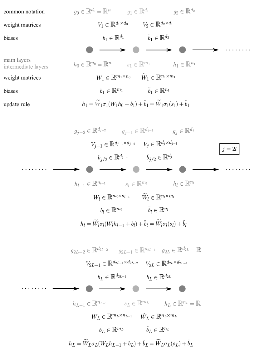
Figure 3.1: Structure of a classical feed-forward neural network with update rule (3.1) in standard notation $(l\in\{0,\ldots,L\})$ and in common notation $(j\in\{0,\ldots,2L\})$ for main and intermediate layers, visualized in dark and light gray respectively.

A classical feed-forward neural network is structured in main layers $h_{l}$, $l\in\{0,1,.\ldots,L\}$, $L\geq 1$ with width $n_{l}$, i.e. $h_{l}\in\mathbb{R}^{n_{l}}$. The network is initialized by input data $h_{0}=x\in\mathcal{X}$, $\mathcal{X}\subset\mathbb{R}^{n}$ open with $n\coloneqq n_{0}$ and the layers are for $l\in\{1,\ldots,L\}$ iteratively updated by

$$h_{l}=\widetilde{W}_{l}\sigma_{l}(W_{l}h_{l-1}+b_{l})+\tilde{b}_{l}=\widetilde{W}_{l}\sigma_{l}(s_{l})+\tilde{b}_{l},$$ (3.1)

where $\widetilde{W}_{l}\in\mathbb{R}^{n_{l}\times m_{l}}$ and $W_{l}\in\mathbb{R}^{m_{l}\times n_{l-1}}$ are weight matrices, $b_{l}\in\mathbb{R}^{m_{l}}$ and $\tilde{b}_{l}\in\mathbb{R}^{n_{l}}$ are biases and $\sigma_{l}:\mathbb{R}^{m_{l}}\rightarrow\mathbb{R}^{m_{l}}$ is a component-wise applied activation function, i.e. $\sigma_{l}=([\sigma_{l}]_{1},\ldots,[\sigma_{l}]_{m_{l}})^{\top}$ with $[\sigma_{l}]_{i}:\mathbb{R}\rightarrow\mathbb{R}$ for $i\in\{1,\ldots,m_{l}\}$. $m_{l}$ is the dimension of the intermediate layers $s_{l}\coloneqq W_{l}h_{l-1}+b_{l}$, $l\in\{1,\ldots,L\}$ to which the activation function $\sigma$ is applied. For an easier notation, we additionally enumerate the main and intermediate layers together by $g_{j}\in\mathbb{R}^{d_{j}}$, $j\in\{0,\ldots,2L\}$, where $g_{2l}=h_{l}\in\mathbb{R}^{d_{2l}}=\mathbb{R}^{n_{l}}$ for $l\in\{0,\ldots,L\}$ and $g_{2l-1}=s_{l}\in\mathbb{R}^{d_{2l-1}}=\mathbb{R}^{m_{l}}$ for $l\in\{1,\ldots,L\}$. Additionally we enumerate the weight matrices together by $V_{j}\in\mathbb{R}^{d_{j}\times d_{j-1}}$, $j\in\{1,\ldots,2L\}$, such that $(W_{1},\widetilde{W}_{1},\ldots,W_{L},\widetilde{W}_{L})=(V_{1},\ldots,V_{2L})$ with $W_{l}=V_{2l-1}$ and $\widetilde{W}_{l}=V_{2l}$ for $l\in\{1,\ldots,L\}$. The output of the neural network is the last layer $h_{L}$. The structure of the neural network is visualized in Figure 3.1. The general neural network update rule (3.1) contains feed-forward neural networks with an outer nonlinearity

$$h_{l}=\sigma_{l}(W_{l}h_{l-1}+b_{l})$$

by choosing $m_{l}=n_{l}$, $\widetilde{W}_{l}=\textup{Id}_{n_{l}}$ and $\tilde{b}_{l}=0$ for $l\in\{1,\ldots,L\}$ and feed-forward neural networks with an inner nonlinearity

$$h_{l}=\widetilde{W}_{l}\sigma_{l}(h_{l-1})+\tilde{b}_{l}$$

by choosing $m_{l}=n_{l-1}$, $W_{l}=\textup{Id}_{n_{l-1}}$ and $b_{l}=0$ for $l\in\{1,\ldots,L\}$. Both architectures, with outer and inner nonlinearity, as well as their combination with update rule (3.1) are well-known in machine learning theory [5]. The distinction between the different types of nonlinearities also exists in classical neural field models of mathematical neuroscience: the class of Wilson-Cowan models has outer nonlinearities and the class of Amari models has inner nonlinearities [4].

In the main theorems of this work we assume, that all components of $\sigma_{l}$ are continuous and strictly monotone on $\mathbb{R}$, i.e. $[\sigma_{l}]_{i}^{\prime}>0$ or $[\sigma_{l}]_{i}^{\prime}<0$ on $\mathbb{R}$ in the case that $[\sigma_{l}]_{i}$ is differentiable, $i\in\{1,\ldots,m_{l}\}$. As we restrict our analysis to single components of the output, we can without loss of generality assume that the output $h_{L}\in\mathbb{R}$ is one-dimensional, i.e. $n_{L}=1$. Hence, the neural network mapping $h_{0}$ to $h_{L}$ is a function $\Phi:\mathcal{X}\rightarrow\mathbb{R}$.

Lemma 3.1.

Let $\Phi:\mathcal{X}\rightarrow\mathbb{R}$, $\mathcal{X}\subset\mathbb{R}^{n}$ be a classical feed-forward neural network with update rule (3.1). If the activation functions fulfill for $l\in\{1,\ldots,L\}$, $i\in\{1,\ldots,m_{l}\}$ that $[\sigma_{l}]_{i}\in C^{k}(\mathbb{R},\mathbb{R})$ with $k\geq 0$, then $\Phi\in C^{k}(\mathcal{X},\mathbb{R})$.

Proof.

As a composition of $k$ times continuously differentiable functions, the chain rule implies that also $\Phi$ is $k$ times continuously differentiable. ∎

Definition 3.2.

For $k\geq 0$, the set of all classical feed-forward neural networks $\Phi:\mathcal{X}\rightarrow\mathbb{R}$, $\mathcal{X}\subset\mathbb{R}^{n}$ open with update rule (3.1) and component-wise applied strictly monotone activation functions $[\sigma_{l}]_{i}\in C^{k}(\mathbb{R},\mathbb{R})$, $l\in\{1,\ldots,L\}$, $i\in\{1,\ldots,m_{l}\}$ is denoted by $\Xi^{k}(\mathcal{X},\mathbb{R})\subset C^{k}(\mathcal{X},\mathbb{R})$.

The set of neural networks $\Xi^{k}(\mathcal{X},\mathbb{R})$ we study in this work is larger than the feed-forward neural networks considered in the work by Kurochkin [16], where the analysis is restricted to outer nonlinearities with strictly monotonically increasing activation functions. For most of the upcoming theorems we provide for illustration purposes low-dimensional examples. If explicit calculations of gradients and Hessian matrices are needed in the examples, we work with the soft-plus action function $\sigma(x)=\ln(1+\exp(x))$, which has as first derivative the sigmoid function $\sigma^{\prime}(x)=\frac{1}{1+\exp(-x)}$.

3.1 Special Architectures

In the following, we subdivide the set of all classical feed-forward neural networks $\Xi^{k}(\mathcal{X},\mathbb{R})$ introduced in Definition 3.2 in three different classes: non-augmented neural networks, augmented neural networks and neural networks with a bottleneck.

Non-Augmented

We call a classical feed-forward neural network $\Phi\in\Xi^{k}(\mathcal{X},\mathbb{R})$ non-augmented, if it holds for the widths of the layers that $d_{j}\leq n$ for $j\in\{0,\ldots,2L\}$. The space is non-augmented, as all layers have a width smaller or equal to the width $n$ of the layer $h_{0}$, which corresponds to the input data $x\in\mathcal{X}\subset\mathbb{R}^{n}$. Additionally we require, that the widths of the layers are monotonically decreasing from layer to layer, i.e. $d_{j-1}\geq d_{j}$ for $j\in\{1,\ldots,2L\}$. The subset of non-augmented neural networks is denoted by

$$\Xi^{k}_{\textup{N}}(\mathcal{X},\mathbb{R})\coloneqq\left\{\Phi\in\Xi^{k}(\mathcal{X},\mathbb{R}):\Phi\textup{ is non-augmented}\right\}.$$

Augmented

We call a classical feed-forward neural network $\Phi\in\Xi^{k}(\mathcal{X},\mathbb{R})$ augmented, if the first layer of maximal width $g_{l^{\ast}}$ has at least $n+1$ nodes, i.e. $d_{l^{\ast}}\geq n+1$ and $d_{l^{\ast}-1}<d_{l^{\ast}}$. The space is augmented, as there exists a layer with width larger than the dimension of the input data $x\in\mathbb{R}^{n}$. Furthermore we require, that between layer $g_{0}$ and $g_{l^{\ast}}$, the width of the layers is monotonically increasing, i.e. $d_{j-1}\leq d_{j}$ for $0<j\leq l^{\ast}$ and between layer $g_{l^{\ast}}$ and $g_{2L}$, the width of the layers is monotonically decreasing, i.e. $d_{j-1}\geq d_{j}$ for $l^{\ast}<j\leq 2L$. The subset of augmented neural networks is denoted by

$$\Xi^{k}_{\textup{A}}(\mathcal{X},\mathbb{R})\coloneqq\left\{\Phi\in\Xi^{k}(\mathcal{X},\mathbb{R}):\Phi\textup{ is augmented}\right\}.$$

Bottleneck

We say that a classical feed-forward neural network $\Phi\in\Xi^{k}(\mathcal{X},\mathbb{R})$ has a bottleneck in layer $g_{j^{\ast}}$, if there exists three layers $g_{i^{\ast}}$, $g_{j^{\ast}}$ and $g_{l^{\ast}}$ with $0\leq i^{\ast}<j^{\ast}<l^{\ast}\leq 2L$, such that $d_{i^{\ast}}>d_{j^{\ast}}$ and $d_{j^{\ast}}<d_{l^{\ast}}$. Typical neural network architectures which have a bottleneck are auto-encoders, where the dimension is first reduced to extract specific features and then augmented again to the dimension of the initial data. The subset of non-augmented neural networks is denoted by

$$\Xi^{k}_{\textup{B}}(\mathcal{X},\mathbb{R})\coloneqq\left\{\Phi\in\Xi^{k}(\mathcal{X},\mathbb{R}):\Phi\textup{ has a bottleneck}\right\}.$$

The three different types of feed-forward neural networks are visualized in Figure 3.2. In the following we show that these three types of architectures build a disjoint subdivision of all classical feed-forward neural networks.

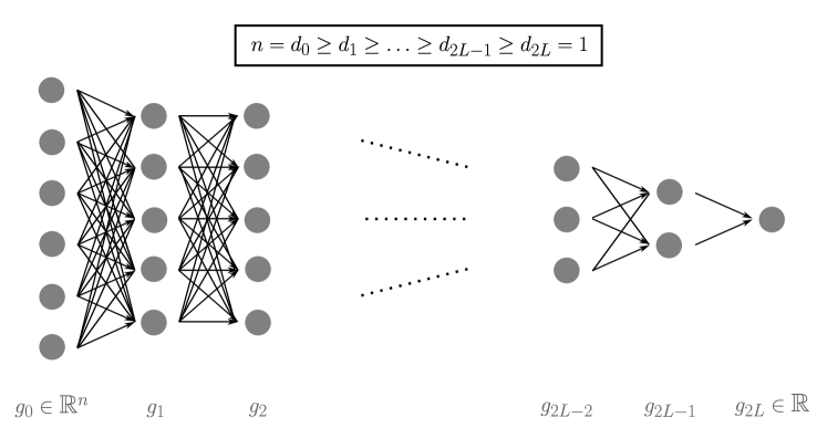
(a) Structure of a non-augmented neural network $\Phi\in\Xi_{\textup{N}}^{k}(\mathcal{X},\mathbb{R})$.

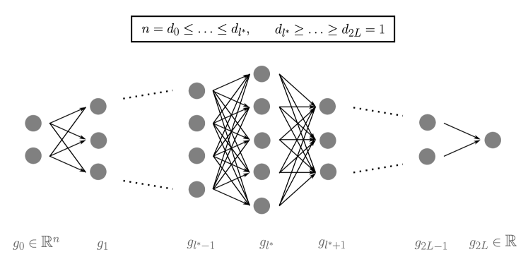
(b) Structure of an augmented neural network $\Phi\in\Xi_{\textup{A}}^{k}(\mathcal{X},\mathbb{R})$.

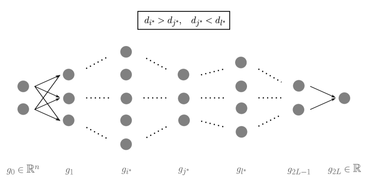
(c) Structure of a neural network with a bottleneck $\Phi\in\Xi_{\textup{B}}^{k}(\mathcal{X},\mathbb{R})$.

Figure 3.2: The three different types of architectures non-augmented, augmented and bottleneck for classical feed-forward neural networks $\Phi\in\Xi^{k}(\mathcal{X},\mathbb{R})$.

Proposition 3.3.

The subdivision of classical feed-forward neural networks $\Xi^{k}(\mathcal{X},\mathbb{R})$ in non-aug-mented neural networks $\Xi^{k}_{\textup{N}}(\mathcal{X},\mathbb{R})$, augmented neural networks $\Xi^{k}_{\textup{A}}(\mathcal{X},\mathbb{R})$ and neural networks with a bottleneck $\Xi^{k}_{\textup{B}}(\mathcal{X},\mathbb{R})$, is a complete partition in three disjoint sub-classes of feed-forward neural networks, i.e.

$$\Xi^{k}(\mathcal{X},\mathbb{R})=\Xi^{k}_{\textup{N}}(\mathcal{X},\mathbb{R})\;\dot{\cup}\;\,\Xi^{k}_{\textup{A}}(\mathcal{X},\mathbb{R})\;\dot{\cup}\;\,\Xi^{k}_{\textup{B}}(\mathcal{X},\mathbb{R}).$$

Proof.

We define the three index sets

$$\mathcal{A}_{<} \coloneqq\left\{j\in\{1,\ldots,2L\}:d_{j-1}<d_{j}\right\},$$

$$\mathcal{A}_{=} \coloneqq\left\{j\in\{1,\ldots,2L\}:d_{j-1}=d_{j}\right\},$$

$$\mathcal{A}_{>} \coloneqq\left\{j\in\{1,\ldots,2L\}:d_{j-1}>d_{j}\right\},$$

which are a disjoint subdivision of all indices, i.e. $\mathcal{A}_{<}\,\dot{\cup}\,\mathcal{A}_{=}\,\dot{\cup}\,\mathcal{A}_{>}=\{1,...,2L\}$. We distinguish now different cases depending on the partition of the indices in the sets $\mathcal{A}_{<}$, $\mathcal{A}_{=}$ and $\mathcal{A}_{>}$.

• Case 1: $\mathcal{A}_{<}=\varnothing$. In this case it holds $d_{j-1}\geq d_{j}$ for all $j\in\{1,\ldots,2L\}$. As $d_{0}=n$ this implies that $d_{j}\leq n$ for all $j\in\{0,\ldots,2L\}$. By definition, the feed-forward neural network is non-augmented.

• Case 2: $\mathcal{A}_{<}\neq\varnothing$. As the set $\mathcal{A}_{<}$ is finite, there exists a maximal element $l^{\ast}=\max\{j:j\in\mathcal{A}_{<}\}$.

• Case 2.1: $\mathcal{A}_{<}\neq\varnothing$ and $\{1,\ldots,l^{\ast}\}\subset\left(\mathcal{A}_{<}\cup\mathcal{A}_{=}\right)$. In this case it holds $d_{j-1}\leq d_{j}$ for $0<j\leq l^{\ast}$. This implies $d_{l^{\ast}}>d_{l^{\ast}-1}\geq\ldots\geq d_{0}=n$, hence $d_{l^{\ast}}\geq n+1$. As $l^{\ast}=\max\{j:j\in\mathcal{A}_{<}\}$ it holds $\{l^{\ast}+1,\ldots,2L\}\subset\left(\mathcal{A}_{=}\cup\mathcal{A}_{>}\right)$. Consequently $d_{j-1}\geq d_{j}$ for $l^{\ast}<j\leq 2L$. By definition, the feed-forward neural network is augmented.

• Case 2.2: $\mathcal{A}_{<}\neq\varnothing$ and $\{1,\ldots,l^{\ast}\}\not\subset\left(\mathcal{A}_{<}\cup\mathcal{A}_{=}\right)$. Define now the index $j^{\ast}$ as the maximal element of $\{1,\ldots,l^{\ast}\}$ which is not contained in $\mathcal{A}_{<}\cup\mathcal{A}_{=}$: $j^{\ast}=\max\{j\in\{1,\ldots,l^{\ast}\}:j\in\mathcal{A}_{>}\}$. It holds $j^{\ast}<l^{\ast}$ as $l^{\ast}\in\mathcal{A}_{<}$. For $i^{\ast}=j^{\ast}-1$ it holds $0\leq i^{\ast}<j^{\ast}<l^{\ast}\leq 2L$ and $d_{i^{\ast}}=d_{j^{\ast}-1}>d_{j^{\ast}}$. As $\{j^{\ast}+1,\ldots,l^{\ast}\}\subset\mathcal{A}_{<}\cup\mathcal{A}_{=}$ and $l^{\ast}\in\mathcal{A}_{<}$ it also holds $d_{j^{\ast}}\leq\ldots\leq d_{l^{\ast}-1}<d_{l^{\ast}}$. This implies that the considered feed-forward neural network has a bottleneck as $d_{i^{\ast}}>d_{j^{\ast}}$ and $d_{j^{\ast}}<d_{l^{\ast}}$.

As the three cases 1, 2.1 and 2.2 are a complete and disjoint subdivision of possible partitions of the indices $1,\ldots,2L$ in the sets $\mathcal{A}_{<}$, $\mathcal{A}_{=}$ and $\mathcal{A}_{>}$, also the subdivision of classical feed-forward neural networks $\Xi^{k}(\mathcal{X},\mathbb{R})$ in non-augmented neural networks $\Xi^{k}_{\textup{N}}(\mathcal{X},\mathbb{R})$, augmented neural network $\Xi^{k}_{\textup{A}}(\mathcal{X},\mathbb{R})$ and neural networks with a bottleneck $\Xi^{k}_{\textup{B}}(\mathcal{X},\mathbb{R})$ is a complete partition in three disjoint sub-classes of feed-forward neural networks. ∎

3.2 Equivalent Neural Network Architectures

In this section, we first define the weight and bias spaces for classical feed-forward neural networks. Afterwards, we introduce a definition of equivalent neural network architectures and show via an explicit algorithm how to obtain under all equivalent neural networks architectures the one with the fewest number of nodes. The resulting architecture has only full rank matrices and is called the normal form of the neural network, which is used in the following Sections 3.3 and 3.4.

To define the weight space, we identify a matrix in $\mathbb{R}^{p\times q}$ with a point in $\mathbb{R}^{pq}$ by stacking the columns of the matrix. This operation is also known as vectorization.

Definition 3.4 ([18]).

Let $A\in\mathbb{R}^{p\times q}$ be a matrix and denote the $j$-th column by $a_{j}\in\mathbb{R}^{p}$, $j\in\{1,\ldots,q\}$. Then the bijective vectorization operator $\textup{vec}:\mathbb{R}^{p\times q}\rightarrow\mathbb{R}^{pq}$ is defined as

$$\textup{vec}(A)=\begin{pmatrix}a_{1}\\ \vdots\\ a_{q}\end{pmatrix}$$

with inverse $\textup{vec}^{-1}:\mathbb{R}^{pq}\rightarrow\mathbb{R}^{p\times q}$.

In the following, we define weight and bias spaces for classical feed-forward neural networks, generalize the vectorization operator of Definition 3.4 to multiple weight matrices and introduce a stacking operator for biases.

Definition 3.5.

Let $\Phi\in\Xi^{k}(\mathcal{X},\mathbb{R})$, $k\geq 0$ be a classical feed-forward neural network with weight matrices $W=(W_{1},\widetilde{W}_{1},\ldots,W_{L},\widetilde{W}_{L})=(V_{1},\ldots,V_{2L})$ and biases $b=(b_{1},\tilde{b}_{1}\ldots,b_{L},\tilde{b}_{L})$.

1. The weight space $\mathbb{W}$ is defined as the space of all weight matrices,

   $$\mathbb{W} \coloneqq\mathbb{R}^{m_{1}\times n_{0}}\times\mathbb{R}^{n_{1}\times m_{1}}\times\ldots\times\mathbb{R}^{m_{L}\times n_{L-1}}\times\mathbb{R}^{n_{L}\times m_{L}}$$

   $$=\mathbb{R}^{d_{1}\times d_{0}}\times\mathbb{R}^{d_{2}\times d_{1}}\times\ldots\times\mathbb{R}^{d_{2L-1}\times d_{2L-2}}\times\mathbb{R}^{d_{2L}\times d_{2L-1}}.$$

2. For $W\in\mathbb{W}$ the bijective multiple vectorization operator $\textup{vecm}:\mathbb{W}\rightarrow\mathbb{R}^{N_{W}}$ with $N_{W}\coloneqq\sum_{l=1}^{L}m_{l}(n_{l-1}+n_{l})=\sum_{l=1}^{2L}d_{l}d_{l-1}$ is defined as

   $$\textup{vecm}(W)\coloneqq\begin{pmatrix}\textup{vec}(W_{1})\\ \vdots\\ \textup{vec}(\widetilde{W}_{L})\end{pmatrix}=\begin{pmatrix}\textup{vec}(V_{1})\\ \vdots\\ \textup{vec}(V_{2L})\end{pmatrix}\in\mathbb{R}^{N_{W}}.$$

   The inverse of the operator vecm is denoted by $\textup{vecm}^{-1}:\mathbb{R}^{N_{W}}\rightarrow\mathbb{W}$.

3. The subset of the weight space $\mathbb{W}$, in which all weight matrices $W$ have full rank is denoted by

   $$\mathbb{W}^{\ast}\coloneqq \Bigl{\{}W\in\mathbb{W}:\textup{ rank}(W_{l})=\min\{m_{l},n_{l-1}\},\textup{ rank}(\widetilde{W}_{l})=\min\{m_{l},n_{l}\}\;\forall\;l\in\{1,\ldots,L\}\Bigr{\}}$$

   $$= \Bigl{\{}W\in\mathbb{W}:\textup{ rank}(V_{j})=\min\{d_{j},d_{j-1}\}\;\forall\;j\in\{1,\ldots,2L\}\Bigr{\}}.$$

   The set of classical feed-forward neural networks $\Phi\in\Xi^{k}_{i}(\mathcal{X},\mathbb{R})$, $i\in\{\varnothing,\textup{N},\textup{A},\textup{B}\}$ with weight matrices $W\in\mathbb{W}^{\ast}$ is denoted by $\Xi^{k}_{i,\mathbb{W}^{\ast}}(\mathcal{X},\mathbb{R})$.

4. The bias space $\mathbb{B}$ is defined as the space of all biases $b=(b_{1},\tilde{b}_{1}\ldots,b_{L},\tilde{b}_{L})$,

   $$\mathbb{B}\coloneqq\mathbb{R}^{m_{1}}\times\mathbb{R}^{n_{1}}\times\ldots\times\mathbb{R}^{m_{L}}\times\mathbb{R}^{n_{L}}=\mathbb{R}^{d_{1}}\times\mathbb{R}^{d_{2}}\times\ldots\times\mathbb{R}^{d_{2L-1}}\times\mathbb{R}^{d_{2L}}.$$

5. For $b=(b_{1},\tilde{b}_{1}\ldots,b_{L},\tilde{b}_{L})\in\mathbb{B}$ the bijective stacking operator $\textup{stk}:\mathbb{B}\rightarrow\mathbb{R}^{N_{B}}$ with $N_{B}\coloneqq\sum_{l=1}^{L}(m_{l}+n_{l})=\sum_{l=1}^{2L}d_{l}$ is defined as

   $$\textup{stk}(b)\coloneqq\begin{pmatrix}b_{1}\\ \vdots\\ b_{L}\end{pmatrix}\in\mathbb{R}^{N_{B}}.$$

   The inverse of the operator stk is denoted by $\textup{stk}^{-1}:\mathbb{R}^{N_{B}}\rightarrow\mathbb{B}$.

The following lemma shows, that the subset of all weight matrices $W\in\mathbb{W}$, where at least one matrix has not full rank, i.e. the set $\mathbb{W}\setminus\mathbb{W}^{\ast}$, is a zero set with respect to the Lebesgue measure in the identified space $\mathbb{R}^{N_{W}}$.

Lemma 3.6.

For all weights $w\in\mathbb{R}^{N_{W}}$, except possibly for a zero set in $\mathbb{R}^{N_{W}}$ w.r.t. the Lebesgue measure, all corresponding weight matrices $W=\textup{vecm}^{-1}(w)$ have full rank, i.e. the set

$$\textup{vecm}(\mathbb{W}\setminus\mathbb{W}^{\ast})\coloneqq\left\{\textup{vecm}(W)\in\mathbb{R}^{N_{W}}:W\in\mathbb{W}\setminus\mathbb{W}^{\ast}\right\}$$

is a zero set in $\mathbb{R}^{N_{W}}$.

Proof.

By [22, Theorem 5.15], the set of $p\times q$ matrices with rank $k$

$$M_{p,q,k}\coloneqq\left\{M\in\mathbb{R}^{p\times q}:\textup{rank}(M)=k\right\}\subset\mathbb{R}^{p\times q},$$

is in the identified space $\mathbb{R}^{pq}$ a manifold of dimension $k(p+q-k)$. For matrices which do not have full rank, i.e. the rank $k$ fulfills $k<k^{\ast}\coloneqq\min\{p,q\}$, the dimension of $M_{p,q,k}$ is strictly smaller than $pq$ as for $k=k^{\ast}-i$, $i\geq 1$ it holds

$$k(p+q-k) =(k^{\ast}-i)(p+q-k^{\ast}+i)=(\min\{p,q\}-i)(\max\{p,q\}+i)$$

$$=pq-i(\max\{p,q\}-\min\{p,q\})-i^{2}<pq.$$

Consequently $\textup{vec}(M_{p,q,k})\coloneqq\{\textup{vec}(M)\in\mathbb{R}^{pq}:M\in M_{p,q,k}\}$ has for $k<k^{\ast}$ Lebesgue measure zero in $\mathbb{R}^{pq}$. We denote the set of all matrices, which do not have full rank by

$$M_{p,q,k<k^{\ast}}\coloneqq\bigcup_{k=0}^{k^{\ast}-1}M_{p,q,k}.$$

Since

$$\textup{vec}(M_{p,q,k<k^{\ast}})=\textup{vec}\left(\bigcup_{k=0}^{k^{\ast}-1}M_{p,q,k}\right)=\bigcup_{k=0}^{k^{\ast}-1}\textup{vec}(M_{p,q,k})$$

is a finite union of sets of Lebesgue measure zero in $\mathbb{R}^{pq}$, the Lebesgue measure of $\textup{vec}(M_{p,q,k<k^{\ast}})$ is also zero in $\mathbb{R}^{pq}$. Transferred to the weight space $\mathbb{W}$ it follows that for $j\in\{1,\ldots,2L\}$, the set

$$\textup{vecm}\left(\mathbb{R}^{d_{1}\times d_{0}}\times\ldots\times\mathbb{R}^{d_{j-1}\times d_{j-2}}\times M_{d_{j},d_{j-1},k<k^{\ast}(j)}\times\mathbb{R}^{d_{j+1}\times d_{j}}\times\ldots\times\mathbb{R}^{d_{2L}\times d_{2L-1}}\right)$$

is a zero set w.r.t. the Lebesgue measure in $\mathbb{R}^{N_{W}}$. Hereby $k^{\ast}(j)=\min\{d_{j},d_{j-1}\}$ denotes the maximal rank of a matrix in $\mathbb{R}^{d_{j}\times d_{j-1}}$. Consequently also the finite union

$$\textup{vecm}(\mathbb{W}\setminus\mathbb{W}^{\ast})$$

$$=\; \textup{vecm}\left(\bigcup_{j=1}^{2L}\mathbb{R}^{d_{1}\times d_{0}}\times\ldots\times\mathbb{R}^{d_{j-1}\times d_{j-2}}\times M_{d_{j},d_{j-1},k<k^{\ast}(j)}\times\mathbb{R}^{d_{j+1}\times d_{j}}\times\ldots\times\mathbb{R}^{d_{2L}\times d_{2L-1}}\right)$$

$$=\; \bigcup_{j=1}^{2L}\textup{vecm}\Big{(}\mathbb{R}^{d_{1}\times d_{0}}\times\ldots\times\mathbb{R}^{d_{j-1}\times d_{j-2}}\times M_{d_{j},d_{j-1},k<k^{\ast}(j)}\times\mathbb{R}^{d_{j+1}\times d_{j}}\times\ldots\times\mathbb{R}^{d_{2L}\times d_{2L-1}}\Big{)}$$

is a zero set w.r.t. the Lebesgue measure in $\mathbb{R}^{N_{W}}$. This implies that the set of weights $w\in\mathbb{R}^{N_{W}}$, where at least one of the weight matrices of $W=\textup{vecm}^{-1}(w)$ has not full rank is a zero set in $\mathbb{R}^{N_{W}}$ w.r.t. the Lebesgue measure and the result follows. ∎

A first reason to study mainly feed-forward neural networks with full rank weight matrices is that the set of full rank matrices has full measure in $\mathbb{R}^{N_{W}}$. A second reason is, that every classical feed-forward neural network, which has at least one non-full rank weight matrix, is equivalent to a classical feed-forward neural network with less nodes and only full rank matrices. By equivalent we mean, that both neural network architectures have the same output for every input $x\in\mathcal{X}$.

Definition 3.7.

Let $k\geq 0$ and $\Phi\in\Xi^{k}(\mathcal{X},\mathbb{R})$ be a classical feed-forward neural network. We call another classical feed-forward neural network $\overline{\Phi}\in\Xi^{k}(\mathcal{X},\mathbb{R})$ equivalent to $\Phi$ if $\Phi(x)=\overline{\Phi}(x)$ for all $x\in\mathcal{X}$. We say that the neural network $\overline{\Phi}$ has a smaller (larger) architecture than $\Phi$ if the number of nodes per layer fulfills $\overline{d}_{j}\leq d_{j}$ ($\overline{d}_{j}\geq d_{j}$) for $j\in\{0,\ldots,2L\}$ and the total number of nodes is strictly smaller (larger), i.e. $\overline{N}_{B}<N_{B}$ ($\overline{N}_{B}>N_{B}$). It is possible that the number of layers $\overline{L}$ of $\overline{\Phi}$ is smaller than the number of layers $L$ in $\Phi$, then we set $\overline{d}_{j}=0$ for $j\in\{2\overline{L}+1,\ldots,2L\}$.

We always denote the equivalent neural network and all corresponding weight matrices, biases and dimensions with an overbar. In the following Lemmas 3.8 and 3.9, we study feed-forward neural networks, which have at least one non-full rank matrix and explicitly construct an equivalent neural network, where the considered matrix has full rank. Afterwards we show in Theorem 3.12, how to combine the two Lemmas to construct an equivalent neural network architecture with weight matrices $W\in\mathbb{W}^{\ast}$. First, we consider the case that an inner weight matrix $W_{l+1}\in\mathbb{R}^{m_{l+1}\times n_{l}}$ has not full rank for some $l\in\{1,\ldots,L-1\}$ and show that the feed-forward neural network is equivalent to a network with a smaller architecture, which fulfills certain rank properties.

Lemma 3.8.

Let $\Phi\in\Xi^{k}_{\mathbb{W}\setminus\mathbb{W}^{\ast}}(\mathcal{X},\mathbb{R})$ with a non-zero, non-full rank matrix $W_{l+1}\in\mathbb{R}^{m_{l+1}\times n_{l}}$ for some $l\in\{1,\ldots,L-1\}$, i.e. $0<\textup{rank}(W_{l+1})<\min\{m_{l+1},n_{l}\}$. Then there exists an equivalent feed-forward neural network $\overline{\Phi}\in\Xi^{k}(\mathcal{X},\mathbb{R})$ with smaller architecture. Especially only the number of nodes in layer $h_{l}$ is reduced by one, i.e. $\overline{n}_{l}=n_{l}-1\geq 1$, and $W_{l+1}$, $\widetilde{W}_{l}$ and $\tilde{b}_{l}$ are replaced by new matrices $\overline{W}_{l+1}\in\mathbb{R}^{m_{l+1}\times\overline{n}_{l}}$ and $\overline{\widetilde{W}}_{l}\in\mathbb{R}^{\overline{n}_{l}\times m_{l}}$ with $\textup{rank}(\overline{W}_{l+1})=\textup{rank}(W_{l+1})$, $\textup{rank}(\overline{\widetilde{W}}_{l})\leq\textup{rank}(\widetilde{W}_{l})$, $\overline{W}_{l+1}\overline{\widetilde{W}}_{l}=W_{l+1}\widetilde{W}_{l}$ and a new bias $\overline{\tilde{b}}_{l}\in\mathbb{R}^{\overline{n}_{l}}$.

Proof.

If $0<\textup{rank}(W_{l+1})<\min\{m_{l+1},n_{l}\}$ for some $l\in\{1,\ldots,L-1\}$, it holds $m_{l+1},n_{l}\geq 2$. The columns of $W_{l+1}\in\mathbb{R}^{m_{l+1}\times n_{l}}$ are linearly dependent, i.e. for the columns $[W_{l+1}]_{j}\in\mathbb{R}^{m_{l+1}}$, $j\in\{1,\ldots,n_{l}\}$ there exist scalars $\tilde{\alpha}_{j}$, $j\in\{1,\ldots,n_{l}\}$ not all equal to zero, such that

$$\sum_{j=1}^{n_{l}}\tilde{\alpha}_{j}[W_{l+1}]_{j}=0\in\mathbb{R}^{m_{l+1}}.$$

Since $\tilde{\alpha}_{i}\neq 0$ for some $i\in\{1,\ldots,n_{l}\}$, it holds

$$[W_{l+1}]_{i}=\sum_{j=1,j\neq i}^{n_{l}}\alpha_{j}[W_{l+1}]_{j}$$

with $\alpha_{j}\coloneqq-\tilde{\alpha}_{j}/\tilde{\alpha}_{i}$. If $[W_{l+1}]_{i}=0$ is a zero column, no information of the node $[h_{l}]_{i}$ is transferred to the next layer, which indicates that the neural network $\Phi$ is equivalent to a smaller neural network, where the node $[h_{l}]_{i}$ and all connected weights are removed. In the following we prove this statement for the general case that $[W_{l+1}]_{i}\in\mathbb{R}^{m_{l+1}}$ is a linear combination of the other columns. We define a new neural network $\overline{\Phi}\in\Xi^{k}(\mathcal{X},\mathbb{R})$, which has the same structure, weights, biases and activation functions as $\Phi$, only the number of nodes in layer $h_{l}$ is reduced by one, i.e. $\overline{n}_{l}=n_{l}-1\geq 1$, and $W_{l+1}$, $\widetilde{W}_{l}$ and $\tilde{b}_{l}$ are replaced by new matrices $\overline{W}_{l+1}\in\mathbb{R}^{m_{l+1}\times\overline{n}_{l}}$ and $\overline{\widetilde{W}}_{l}\in\mathbb{R}^{\overline{n}_{l}\times m_{l}}$ and a new bias $\overline{\tilde{b}}_{l}\in\mathbb{R}^{\overline{n}_{l}}$. We define the matrix

$$\overline{W}_{l+1}=\begin{pmatrix}[W_{l+1}]_{1}&\cdots&[W_{l+1}]_{i-1}&[W_{l+1}]_{i+1}\cdots&[W_{l+1}]_{n_{l}}\end{pmatrix}$$

which has the same rank as $W_{l+1}$, as $W_{l+1}$ arises from $\overline{W}_{l+1}$ by adding the new column $[W_{l+1}]_{i}$, which is a linear combination of the other columns and hence does not increase the maximal number of linearly independent columns. Furthermore we define

$$\overline{\widetilde{W}}_{l}=\begin{pmatrix}[\widetilde{W}_{l}]_{1,1}+\alpha_{1}[\widetilde{W}_{l}]_{i,1}&\cdots&[\widetilde{W}_{l}]_{1,m_{l}}+\alpha_{1}[\widetilde{W}_{l}]_{i,m_{l}}\\ \vdots&&\vdots\\ [\widetilde{W}_{l}]_{i-1,1}+\alpha_{i-1}[\widetilde{W}_{l}]_{i,1}&\cdots&[\widetilde{W}_{l}]_{i-1,m_{l}}+\alpha_{i-1}[\widetilde{W}_{l}]_{i,m_{l}}\\ [\widetilde{W}_{l}]_{i+1,1}+\alpha_{i+1}[\widetilde{W}_{l}]_{i,1}&\cdots&[\widetilde{W}_{l}]_{i+1,m_{l}}+\alpha_{i+1}[\widetilde{W}_{l}]_{i,m_{l}}\\ \vdots&&\vdots\\ [\widetilde{W}_{l}]_{n_{l},1}+\alpha_{n_{l}}[\widetilde{W}_{l}]_{i,1}&\cdots&[\widetilde{W}_{l}]_{n_{l},m_{l}}+\alpha_{n_{l}}[\widetilde{W}_{l}]_{i,m_{l}}\end{pmatrix}$$

which has rank smaller or equal to $\textup{rank}(\widetilde{W}_{l})$. To see this, we first apply linear row operations to the matrix $\widetilde{W}_{l}$ by adding to the $j$-th row, $j\in\{1,\ldots,i-1,i+1,\ldots,n_{l}\}$, the $i$-th row multiplied with $\alpha_{j}$ each. The resulting matrix has the same rank as $\widetilde{W}_{l}$. As we obtain now the matrix $\overline{\widetilde{W}}_{l}$ by removing the $i$-th row, it holds $\textup{rank}(\overline{\widetilde{W}}_{l})\leq\textup{rank}(\widetilde{W}_{l})$. Finally the new bias is given by

$$\overline{\tilde{b}}_{l}=\begin{pmatrix}[\tilde{b}_{l}]_{1}+\alpha_{1}[\tilde{b}_{l}]_{i}\\ \vdots\\ [\tilde{b}_{l}]_{i-1}+\alpha_{i-1}[\tilde{b}_{l}]_{i}\\ [\tilde{b}_{l}]_{i+1}+\alpha_{i+1}[\tilde{b}_{l}]_{i}\\ \vdots\\ [\tilde{b}_{l}]_{n_{l}}+\alpha_{n_{l}}[\tilde{b}_{l}]_{i}\end{pmatrix}.$$

As the neural network architectures $\Phi$ and $\overline{\Phi}$ agree in all weights, biases and activation functions until $\sigma_{l}$, it holds

$$\overline{\sigma}_{l}(\overline{s}_{l})=\overline{\sigma}_{l}(\overline{W}_{l}\overline{h}_{l-1}+\overline{b}_{l})=\sigma_{l}(W_{l}h_{l-1}+b_{l})=\sigma_{l}(s_{l}),\qquad\textup{for all }x\in\mathcal{X}.$$

In the following we aim to show that

$$\overline{W}_{l+1}\overline{h}_{l}=\overline{W}_{l+1}\left[\overline{\widetilde{W}}_{l}\overline{\sigma}_{l}(\overline{s}_{l})+\overline{\tilde{b}}_{l}\right]=W_{l+1}\left[\widetilde{W}_{l}\sigma_{l}(s_{l})+\tilde{b}_{l}\right]=W_{l+1}h_{l},$$

which implies with the fact, that the neural network architectures $\Phi$ and $\overline{\Phi}$ agree in the bias $b_{l+1}$ and in all weights, biases and activation functions from $\sigma_{l+1}$ on-wards, that $\Phi$ and $\overline{\Phi}$ are equivalent. We calculate

$$\overline{W}_{l+1}\overline{h}_{l} =\overline{W}_{l+1}\left[\overline{\widetilde{W}}_{l}\overline{\sigma}_{l}(\overline{s}_{l})+\overline{\tilde{b}}_{l}\right]=\overline{W}_{l+1}\left[\overline{\widetilde{W}}_{l}\sigma_{l}(s_{l})+\overline{\tilde{b}}_{l}\right]$$

$$=\overline{W}_{l+1}\overline{\widetilde{W}}_{l}\sigma_{l}(s_{l})+\overline{W}_{l+1}\overline{\tilde{b}}_{l}$$

$$=W_{l+1}\widetilde{W}_{l}\sigma_{l}(s_{l})+W_{l+1}\tilde{b}_{l}=W_{l+1}\left[\widetilde{W}_{l}\sigma_{l}(s_{l})+\tilde{b}_{l}\right]=W_{l+1}h_{l}$$

where we used in the last line that $\overline{W}_{l+1}\overline{\widetilde{W}}_{l}=W_{l+1}\widetilde{W}_{l}$ and $\overline{W}_{l+1}\overline{\tilde{b}}_{l}=W_{l+1}\tilde{b}_{l}$ since

$$\left[\overline{W}_{l+1}\overline{\widetilde{W}}_{l}\right]_{j,k} =\sum_{p=1,p\neq i}^{n_{l-1}}[W_{l+1}]_{j,p}\left[[\widetilde{W}_{l}]_{p,k}+\alpha_{p}[\widetilde{W}_{l}]_{i,k}\right]=\sum_{p=1}^{n_{l-1}}[W_{l+1}]_{j,p}[\widetilde{W}_{l}]_{p,k}=\left[W_{l+1}\widetilde{W}_{l}\right]_{j,k}$$

$$\left[\overline{W}_{l+1}\overline{\tilde{b}}_{l}\right]_{j} =\sum_{p=1,p\neq i}^{n_{l-1}}[W_{l+1}]_{j,p}\left[[\tilde{b}_{l}]_{p}+\alpha_{p}[\tilde{b}_{l}]_{i}\right]=\sum_{p=1}^{n_{l}}[W_{l+1}]_{j,p}[\tilde{b}_{l}]_{p}=\left[W_{l+1}\tilde{b}_{l}\right]_{j}$$

by the assumption on linear dependence of the columns of $W_{l+1}$. ∎

Second, we show that also in the case that an outer weight matrix $\widetilde{W}_{l}\in\mathbb{R}^{m_{l}\times n_{l-1}}$ has for some $l\in\{1,\ldots,L-1\}$ not full rank, the neural network is equivalent to a smaller architecture with certain rank properties.

Lemma 3.9.

Let $\Phi\in\Xi^{k}_{\mathbb{W}\setminus\mathbb{W}^{\ast}}(\mathcal{X},\mathbb{R})$ with a non-zero, non-full rank matrix $\widetilde{W}_{l}\in\mathbb{R}^{n_{l}\times m_{l}}$ for some $l\in\{1,\ldots,L-1\}$, i.e. $0<\textup{rank}(\widetilde{W}_{l})<\min\{m_{l},n_{l}\}$. Then there exists an equivalent feed-forward neural network $\overline{\Phi}\in\Xi^{k}(\mathcal{X},\mathbb{R})$ with smaller architecture. Especially only the number of nodes in layer $h_{l}$ is reduced by one, i.e. $\overline{n}_{l}=n_{l}-1\geq 1$, and $\widetilde{W}_{l}$, $W_{l+1}$ and $\tilde{b}_{l}$ are replaced by new matrices $\overline{\widetilde{W}}_{l}\in\mathbb{R}^{\overline{n}_{l}\times m_{l}}$ and $\overline{W}_{l+1}\in\mathbb{R}^{m_{l+1}\times\overline{n}_{l}}$ with $\textup{rank}(\overline{\widetilde{W}}_{l})=\textup{rank}(\widetilde{W}_{l})$, $\textup{rank}(\overline{W}_{l+1})\leq\textup{rank}(W_{l+1})$, $\overline{W}_{l+1}\overline{\widetilde{W}}_{l}=W_{l+1}\widetilde{W}_{l}$ and a new bias $\overline{\tilde{b}}_{l}\in\mathbb{R}^{\overline{n}_{l}}$. If $W_{l+1}\in\mathbb{R}^{m_{l+1}\times n_{l}}$ has full rank, i.e. $\textup{rank}(W_{l+1})=\min\{m_{l+1},n_{l}\}$, then $\overline{W}_{l+1}$ has also full rank, i.e. $\textup{rank}(\overline{W}_{l+1})=\min\{m_{l+1},\overline{n}_{l}\}$.

Proof.

If $0<\textup{rank}(\widetilde{W}_{l})<\min\{m_{l},n_{l}\}$ for some $l\in\{1,\ldots,L-1\}$, it holds $m_{l},n_{l}\geq 2$. The rows of $\widetilde{W}_{l}\in\mathbb{R}^{n_{l}\times m_{l}}$ are linearly dependent, i.e. for the rows $[\widetilde{W}_{l}^{\top}]_{j}\in\mathbb{R}^{m_{l}}$, $j\in\{1,\ldots,n_{l}\}$ there exist scalars $\tilde{\alpha}_{j}$, $j\in\{1,\ldots,n_{l}\}$ not all equal to zero, such that

$$\sum_{j=1}^{n_{l}}\tilde{\alpha}_{j}[\widetilde{W}_{l}^{\top}]_{j}=0\in\mathbb{R}^{m_{l}}.$$

Since $\tilde{\alpha}_{i}\neq 0$ for some $i\in\{1,\ldots,n_{l}\}$, it holds

$$[\widetilde{W}_{l}^{\top}]_{i}=\sum_{j=1,j\neq i}^{n_{l}}\alpha_{j}[\widetilde{W}_{l}^{\top}]_{j}$$

with $\alpha_{j}\coloneqq-\tilde{\alpha}_{j}/\tilde{\alpha}_{i}$. If $[\widetilde{W}_{l}^{\top}]_{i}=0$ is a zero row, no information of the activated layer $\sigma_{l}(s_{l})$ is transferred to the node $[h_{l}]_{i}$ of the next layer, which indicates that the neural network $\Phi$ is equivalent to a smaller neural network, where the node $[h_{l}]_{i}$ and all connected weights are removed. In the following we prove this statement for the general case that $[\widetilde{W}_{l}^{\top}]_{i}\in\mathbb{R}^{m_{l}}$ is a linear combination of the other rows. We define a new neural network $\overline{\Phi}\in\Xi^{k}(\mathcal{X},\mathbb{R})$, which has the same structure, weights, biases and activation functions as $\Phi$, only the number of nodes in layer $h_{l}$ is reduced by one, i.e. $\overline{n}_{l}=n_{l}-1\geq 1$, and $\widetilde{W}_{l}$, $W_{l+1}$ and $\tilde{b}_{l}$ are replaced by new matrices $\overline{\widetilde{W}}_{l}\in\mathbb{R}^{\overline{n}_{l}\times m_{l}}$ and $\overline{W}_{l+1}\in\mathbb{R}^{m_{l+1}\times\overline{n}_{l}}$ and a new bias $\overline{\tilde{b}}_{l}\in\mathbb{R}^{\overline{n}_{l}}$. We define the matrix

$$\overline{\widetilde{W}}_{l}=\begin{pmatrix}[\widetilde{W}_{l}^{\top}]_{1}^{\top}\\ \vdots\\ [\widetilde{W}_{l}^{\top}]_{i-1}^{\top}\\ [\widetilde{W}_{l}^{\top}]_{i+1}^{\top}\\ \vdots\\ [\widetilde{W}_{l}^{\top}]^{\top}_{n_{l}}\end{pmatrix}$$

which has the same rank as $\widetilde{W}_{l}$, as $\widetilde{W}_{l}$ arises from $\overline{\widetilde{W}}_{l}$ by adding the new row $[\widetilde{W}_{l}^{\top}]^{\top}_{i}$, which is a linear combination of the other rows and hence does not increase the maximal number of linearly independent rows. Furthermore we define

$$\overline{W}_{l+1}= \left([W_{l+1}]_{1}+\alpha_{1}[W_{l+1}]_{i},\ldots,[W_{l+1}]_{i-1}+\alpha_{i-1}[W_{l+1}]_{i},\right.$$

$$\left.[W_{l+1}]_{i+1}+\alpha_{i+1}[W_{l+1}]_{i},\ldots,[W_{l+1}]_{n_{l}}+\alpha_{n_{l}}[W_{l+1}]_{i}\right)$$

which has rank smaller or equal to $\textup{rank}(W_{l+1})$. To see this, we first apply linear column operations to the matrix $W_{l+1}$ by adding to the $j$-th column, $j\in\{1,\ldots,i-1,i+1,\ldots,n_{l}\}$, the $i$-th column multiplied with $\alpha_{j}$ each. The resulting matrix $Y_{l+1}$ has the same rank as $W_{l+1}$ and $\overline{W}_{l+1}$ is obtained from $Y_{l+1}$ by removing the $i$-th column, hence $\textup{rank}(\overline{W}_{l+1})\leq\textup{rank}(Y_{l+1})=\textup{rank}(W_{l+1})$. If $W_{l+1}$ has full rank, i.e. $\textup{rank}(W_{l+1})=\min\{m_{l+1},n_{l}\}$, then also $\overline{W}_{l+1}$ has full rank, i.e. $\textup{rank}(\overline{W}_{l+1})=\min\{m_{l+1},\overline{n}_{l}\}$. To see this, we distinguish two cases: if $m_{l+1}<n_{l}$ it holds $\textup{rank}(W_{l+1})=m_{l+1}$, such that each $m_{l+1}$ columns of $W_{l+1}$ and hence also of $Y_{l+1}$ are linearly independent. Consequently removing one of the $n_{l}$ columns of $Y_{l+1}$ does not change the rank, such that $\textup{rank}(\overline{W}_{l+1})=m_{l+1}=\min\{m_{l+1},\overline{n}_{l}\}$. If $m_{l+1}\geq n_{l}$ it holds $\textup{rank}(W_{l+1})=n_{l}$, such that all $n_{l}$ columns of $W_{l+1}$ and hence also all $\bar{n}_{l}$ columns of $Y_{l+1}$ are linearly independent. As $Y_{l+1}$ has $n_{l}$ columns, removing one leads to a matrix with $\overline{n}_{l}=n_{l}-1$ linearly independent columns. Consequently it holds $\textup{rank}(\overline{W}_{l+1})=\overline{n}_{l}=\min\{m_{l+1},\overline{n}_{l}\}$. Finally the new bias is given by

$$\overline{\tilde{b}}_{l}=y_{l}+c_{l}\coloneqq\begin{pmatrix}[\tilde{b}_{l}]_{1}\\ \vdots\\ [\tilde{b}_{l}]_{i-1}\\ [\tilde{b}_{l}]_{i+1}\\ \vdots\\ [\tilde{b}_{l}]_{n_{l}}\end{pmatrix}+\begin{pmatrix}[c_{l}]_{1}\\ \vdots\\ [c_{l}]_{i-1}\\ [c_{l}]_{i+1}\\ \vdots\\ [c_{l}]_{n_{l}}\end{pmatrix},$$

where $c_{l}\in\mathbb{R}^{\bar{n}_{l}}$ is an arbitrary solution of the linear system

$$\overline{W}_{l+1}c_{l}=W_{l+1}\tilde{b}_{l}-\overline{W}_{l+1}y_{l}\eqqcolon d_{l}\in\mathbb{R}^{m_{l+1}}.$$

This system has by the Rouché-Capelli Theorem (cf. [25]) always at least one solution as the rank of the matrix $\overline{W}_{l+1}$ is the same as the rank of the extended coefficient matrix

$$\textup{rank}(\overline{W}_{l+1})=\textup{rank}(\overline{W}_{l+1}\big{|}d_{l}).$$

This holds as every column of $W_{l+1}$ is a linear combination of columns of $\overline{W}_{l+1}$, so also the vector $d_{l}$ is a linear combination of the columns of $\overline{W}_{l+1}$. Consequently the maximal number of linearly independent columns does not increase by attaching the vector $d_{l}$ to the matrix $\overline{W}_{l+1}$, such that the rank of $\overline{W}_{l+1}$ and $(\overline{W}_{l+1}\big{|}d_{l})$ is the same. As the neural network architectures $\Phi$ and $\overline{\Phi}$ agree in all weights, biases and activation functions until $\sigma_{l}$, it holds

$$\overline{\sigma}_{l}(\overline{s}_{l})=\overline{\sigma}_{l}(\overline{W}_{l}\overline{h}_{l-1}+\overline{b}_{l})=\sigma_{l}(W_{l}h_{l-1}+b_{l})=\sigma_{l}(s_{l}),\qquad\textup{for all }x\in\mathcal{X}.$$

In the following we aim to show that

$$\overline{W}_{l+1}\overline{h}_{l}=\overline{W}_{l+1}\left[\overline{\widetilde{W}}_{l}\overline{\sigma}_{l}(\overline{s}_{l})+\overline{\tilde{b}}_{l}\right]=W_{l+1}\left[\widetilde{W}_{l}\sigma_{l}(s_{l})+\tilde{b}_{l}\right]=W_{l+1}h_{l},$$

which implies with the fact, that the neural network architectures $\Phi$ and $\overline{\Phi}$ agree in the bias $b_{l+1}$ and in all weights, biases and activation functions from $\sigma_{l+1}$ on-wards, that $\Phi$ and $\overline{\Phi}$ are equivalent. We calculate

$$\overline{W}_{l+1}\overline{h}_{l} =\overline{W}_{l+1}\left[\overline{\widetilde{W}}_{l}\overline{\sigma}_{l}(\overline{s}_{l})+\overline{\tilde{b}}_{l}\right]=\overline{W}_{l+1}\left[\overline{\widetilde{W}}_{l}\sigma_{l}(s_{l})+y_{l}+c_{l}\right]$$

$$=\overline{W}_{l+1}\overline{\widetilde{W}}_{l}\sigma_{l}(s_{l})+\overline{W}_{l+1}y_{l}+\overline{W}_{l+1}c_{l}$$

$$=\overline{W}_{l+1}\overline{\widetilde{W}}_{l}\sigma_{l}(s_{l})+W_{l+1}\tilde{b}_{l}$$

$$=W_{l+1}\widetilde{W}_{l}\sigma_{l}(s_{l})+W_{l+1}\tilde{b}_{l}=W_{l+1}\left[\widetilde{W}_{l}\sigma_{l}(s_{l})+\tilde{b}_{l}\right]=W_{l+1}h_{l},$$

where we used in the last line that $\overline{W}_{l+1}\overline{\widetilde{W}}_{l}=W_{l+1}\widetilde{W}_{l}$ since

$$\left[\overline{W}_{l+1}\overline{\widetilde{W}}_{l}\right]_{j,k}=\sum_{p=1,p\neq i}^{n_{l}}\left([W_{l+1}]_{j,p}+\alpha_{p}[W_{l+1}]_{j,i}\right)[\widetilde{W}_{l}]_{p,k}=\sum_{p=1}^{n_{l}}[W_{l+1}]_{j,p}[\widetilde{W}_{l}]_{p,k}=\left[W_{l+1}\widetilde{W}_{l}\right]_{j,k}$$

by the assumption on linear dependence of the rows of $\widetilde{W}_{l}$. ∎

Finally, we aim to apply Lemma 3.8 and Lemma 3.9 to find smaller equivalent architectures, until all weight matrices of the feed-forward neural network have full rank. To prove this, we need the following two short lemmas.

Lemma 3.10.

Let $A_{1},\ldots,A_{J}$ be matrices $A_{j}\in\mathbb{R}^{k_{j}\times k_{j+1}}$ with full rank, i.e. for $j\in\{1,\ldots,J\}$ it holds $\textup{rank}(A_{j})=\min\{k_{j},k_{j+1}\}$. If the dimensions of the matrices are monotone, i.e. $k_{1}\geq k_{2}\geq\ldots\geq k_{J+1}$ or $k_{1}\leq k_{2}\leq\ldots\leq k_{J+1}$, then also the matrix product

$$A\coloneqq A_{1}A_{2}\ldots A_{J}\in\mathbb{R}^{k_{1}\times k_{J+1}}$$

has full rank, i.e. $\textup{rank}(A)=\min\{k_{1},k_{J+1}\}$.

Proof.

Sylvester’s rank inequality (cf. [26]) implies for the product of two matrices $A_{j}\in\mathbb{R}^{k_{j}\times k_{j+1}}$ and $A_{j+1}\in\mathbb{R}^{k_{j+1}\times k_{j+2}}$ that

$$\textup{rank}(A_{j})+\textup{rank}(A_{j+1})-k_{j+1}\leq\textup{rank}(A_{j}A_{j+1})\leq\min\{k_{j},k_{j+2}\}.$$

If $k_{j}\geq k_{j+1}\geq k_{j+2}$, this implies $\textup{rank}(A_{j}A_{j+1})=k_{j+2}$ and if $k_{j}\leq k_{j+1}\leq k_{j+2}$, this implies $\textup{rank}(A_{j}A_{j+1})=k_{j}$, such that in both cases the matrix product $A_{j}A_{j+1}$ has full rank. Inductively it follows that the matrix product $A$ has full rank, i.e. $\textup{rank}(A)=\min\{k_{1},k_{J+1}\}$. ∎

Lemma 3.11.

Let $A_{0}\in\mathbb{R}^{m\times n}$ with $\textup{rank}(A_{0})>0$. For $i\geq 0$, if $A_{i}\in\mathbb{R}^{m\times(n-i)}$ has not full rank, define iteratively the matrix $A_{i+1}\in\mathbb{R}^{m\times(n-i-1)}$ by removing a column of $A_{i}\in\mathbb{R}^{m\times(n-i)}$ in such a way that $\textup{rank}(A_{i+1})=\textup{rank}(A_{i})$. Then there exists an index $r\geq 0$, such that $A_{r}\in\mathbb{R}^{m\times(n-r)}$ has full rank. The analogous statements holds by iteratively removing the rows of $A_{0}$.

Proof.

Let $p=\textup{rank}(A_{0})<\min\{m,n\}$. By assumption it holds for $i\in\{0,\ldots,n-p-1\}$ that

$$\textup{rank}(A_{i})=\textup{rank}(A_{0})=p,$$

such that $A_{i}\in\mathbb{R}^{m\times(n-i)}$ has not full rank as $p<\min\{m,n-i\}$. Consequently the matrix $A_{n-p}\in\mathbb{R}^{m\times p}$ is well defined and has full rank $p<m$, i.e. the statement holds for $r=n-p$. The statement for iteratively removing the rows of $A_{0}$ follows with the same argumentation for the transpose $A_{0}^{\top}$. ∎

The following theorem is the main reason, why we restrict ourselves to the analysis of neural networks with full rank weight matrices $W\in\mathbb{W}^{\ast}$. It shows, that the neural network is either up to a linear change of coordinates equivalent to a smaller architecture with full rank matrices, or the neural network is a constant function. The resulting architecture is called the normal form of the network.

Theorem 3.12.

Let $\Phi\in\Xi^{k}_{\mathbb{W}\setminus\mathbb{W}^{\ast}}(\mathcal{X},\mathbb{R})$, $k\geq 0$, $\mathcal{X}\subset\mathbb{R}^{n}$ be a classical feed-forward neural network with weight matrices $W=(W_{1},\widetilde{W}_{1},\ldots,W_{L},\widetilde{W}_{L})\in\mathbb{W}\setminus\mathbb{W}^{\ast}$ and biases $b=(b_{1},\tilde{b}_{1},\ldots,b_{L},\tilde{b}_{L})\in\mathbb{B}$.

1. If $\textup{rank}(W_{1})>0$, $\textup{rank}(\widetilde{W}_{L})>0$ and $\textup{rank}(W_{l+1}\widetilde{W}_{l})>0$ for all $l\in\{1,\ldots,L-1\}$, there exists a feed-forward neural network $\overline{\Phi}\in\Xi^{k}_{\mathbb{W}^{\ast}}(\mathcal{Y},\mathbb{R})$, $\mathcal{Y}\subset\mathbb{R}^{\bar{n}}$ for some $\bar{n}\leq n$, which has a smaller architecture, only full rank weight matrices and which is up to a linear change of coordinates, represented by a full rank matrix $A\in\mathbb{R}^{\bar{n}\times n}$, equivalent to $\Phi$. If $\bar{n}=n$, then $A$ is the identity matrix and $\mathcal{Y}=\mathcal{X}$, if $\bar{n}<n$, then $\mathcal{Y}=\{y\in\mathbb{R}^{\bar{n}}:y=Ax,x\in\mathcal{X}\}$.

2. If $\textup{rank}(W_{1})=0$ or $\textup{rank}(\widetilde{W}_{L})=0$ or $\textup{rank}(W_{l+1}\widetilde{W}_{l})=0$ for some $l\in\{1,\ldots,L-1\}$, it holds $\Phi(x)=c_{W,b}$ for all $x\in\mathcal{X}$, where $c_{W,b}$ is a scalar independent of $x$, only depending on $W$ and $b$. $\Phi$ is equivalent to $\overline{\Phi}\in\Xi^{k}(\mathcal{X},\mathbb{R})$ defined by $\overline{L}=1$, $\overline{W}_{1}=0\in\mathbb{R}^{1\times n}$, $\overline{b}_{1}=0\in\mathbb{R}$, $\overline{\widetilde{W}}_{1}=0\in\mathbb{R}$ and $\overline{\tilde{b}}_{1}=c_{W,b}\in\mathbb{R}$, which has a smaller architecture than $\Phi$ if $\overline{\Phi}\neq\Phi$.

Proof.

For case (a) we consider a classical feed-forward neural network $\Phi\in\Xi^{k}_{\mathbb{W}\setminus\mathbb{W}^{\ast}}(\mathcal{X},\mathbb{R})$ and denote its weight matrices by $W^{(0)}=(W_{1}^{(0)},\widetilde{W}_{1}^{(0)},\ldots,W_{L}^{(0)},\widetilde{W}_{L}^{(0)})$ and its input by $x^{(0)}\in\mathcal{X}$. As $W^{(0)}\in\mathbb{W}\setminus\mathbb{W}^{\ast}$, at least one of the weight matrices has not full rank. The assumption $\textup{rank}(W_{1}^{(0)})>0$, $\textup{rank}(\widetilde{W}_{L}^{(0)})>0$ and $\textup{rank}(W_{l+1}^{(0)}\widetilde{W}_{l}^{(0)})>0$ for all $l\in\{1,\ldots,L-1\}$ implies, that all weight matrices of $W^{(0)}$ have at least rank one and every weight matrix, which has not full rank, has at least width and height two. In the following, we explicitly construct equivalent feed-forward neural networks with smaller architectures, until all weight matrices have full rank. The structure of the algorithm is visualized in Figure 3.3. We start with step (i) and $r=0$.

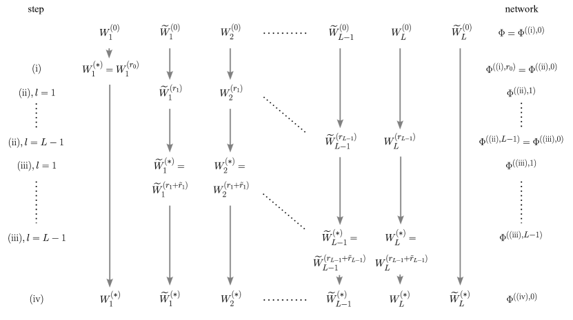
Figure 3.3: Structure of the algorithm defined in the proof of Theorem 3.12(a).

1. If this is the first iteration of step (i), denote the considered feed-forward neural network with weight matrices $(W_{1}^{(0)},\widetilde{W}_{1}^{(0)},W_{2}^{(0)},\ldots,W_{L}^{(0)},\widetilde{W}_{L}^{(0)})$ by $\Phi^{(\textup{(i)},0)}\in\Xi^{k}_{\mathbb{W}\setminus\mathbb{W}^{\ast}}(\mathcal{X},\mathbb{R})$ and set $r=0$.

   If $W_{1}^{(r)}\in\mathbb{R}^{m_{1}\times(n-r)}$ has full rank, go to step (ii) and in the case that $r=0$ set $r_{0}=0$, $W_{1}^{(\ast)}\coloneqq W_{1}^{(r_{0})}=W_{1}^{(0)}$, $\mathcal{Y}\coloneqq\mathcal{X}$, $\Phi^{(\textup{(i)},r_{0})}=\Phi^{(\textup{(i)},0)}$ and define $A\coloneqq\text{Id}_{n}$, which is the identity transformation on $\mathbb{R}^{n}$.

   If $W_{1}^{(r)}\in\mathbb{R}^{m_{1}\times(n-r)}$ has not full rank, it holds $0<\textup{rank}(W_{1}^{(r)})<\min\{m_{1},n-r\}$. The columns of $W_{1}^{(r)}$ are linearly dependent, hence there exist scalars $\tilde{\alpha}_{j}^{(r)}$, $j\in\{1,\ldots,n-r\}$ not all equal to zero, such that

   $$\sum_{j=1}^{n-r}\tilde{\alpha}_{j}^{(r)}[W_{1}^{(r)}]_{j}=0\in\mathbb{R}^{m_{1}}.$$

   Since $\tilde{\alpha}_{i}^{(r)}\neq 0$ for some $i\in\{1,\ldots,n-r\}$, it holds

   $$[W_{1}^{(r)}]_{i}=\sum_{j=1,j\neq i}^{n-r}\alpha_{j}^{(r)}[W_{1}^{(r)}]_{j}$$

   with $\alpha_{j}^{(r)}\coloneqq-\tilde{\alpha}_{j}^{(r)}/\tilde{\alpha}_{i}^{(r)}$. We replace the matrix $W_{1}^{(r)}$ by the matrix

   $$W_{1}^{(r+1)}=\begin{pmatrix}[W_{1}^{(r)}]_{1}&\cdots&[W_{1}^{(r)}]_{i-1}&[W_{1}^{(r)}]_{i+1}\cdots&[W_{1}^{(r)}]_{n-r}\end{pmatrix}\in\mathbb{R}^{m_{1}\times(n-r-1)}$$

   which has the same rank as $W_{1}^{(r)}$, $W_{1}^{(r)}$ arises from $W_{1}^{(r+1)}$ by adding a new column which is a linear combination of the other columns and hence does not increase the maximal number of linearly independent columns. As $\text{rank}(W_{1}^{(r+1)})=\text{rank}(W_{1}^{(r)})$, it holds $\text{rank}(W_{1}^{(r+1)})>0$. Furthermore we make a linear change of coordinates $A^{(r)}:\mathbb{R}^{n-r}\rightarrow\mathbb{R}^{n-r-1}$ of the input data $x^{(r)}\subset\mathbb{R}^{n-r}$ defined by

   $$x^{(r+1)}=A^{(r)}(x^{(r)})=\begin{pmatrix}1&\ldots&0&\alpha_{1}&0&\ldots&0\\ \vdots&&0&\ldots&0&&\vdots\\ 0&\ldots&1&\alpha_{i-1}&0&\ldots&0\\ 0&\ldots&0&\alpha_{i+1}&1&\ldots&0\\ \vdots&&0&\ldots&0&&\vdots\\ 0&\ldots&0&\alpha_{n-r}&0&\ldots&1\end{pmatrix}x^{(r)}=\begin{pmatrix}x_{1}+\alpha_{1}x_{i}\\ \vdots\\ x_{i-1}+\alpha_{i-1}x_{i}\\ x_{i+1}+\alpha_{i+1}x_{i}\\ \vdots\\ x_{n-r}+\alpha_{n-r}x_{i}\end{pmatrix}\in\mathbb{R}^{n-r-1},$$

   such that $W_{1}^{(r)}x^{(r)}=W_{1}^{(r+1)}x^{(r+1)}=W_{1}^{(r+1)}A^{(r)}(x^{(r)})$ for all $x^{(r)}\in\mathbb{R}^{n-r}$. By construction, the matrix $A^{(r)}$ has full rank. The new neural network $\Phi^{(\textup{(i)},r+1)}$ with $W_{1}^{(r)}$ replaced by $W_{1}^{(r+1)}$ and $x^{(r)}$ replaced by $x^{(r+1)}$ is up to the linear change of coordinates $A^{(r)}$ equivalent to $\Phi^{(\textup{(i)},r)}$ and has a smaller architecture.

   If $W_{1}^{(r+1)}$ has full rank, continue with step (ii) and define $r_{0}=r+1$ and

   $$A:\mathbb{R}^{n}\rightarrow\mathbb{R}^{\bar{n}},\quad A\coloneqq A^{(r)}\circ\ldots\circ A^{(0)},$$

   $\mathcal{Y}\coloneqq A(\mathcal{X})\subset\mathbb{R}^{\bar{n}}$, $\bar{n}\coloneqq n-r-1$, and $W_{1}^{(\ast)}\coloneqq W_{1}^{(r_{0})}$. The matrix $A$ has by Lemma 3.10 full rank $\bar{n}$, as all matrices $A^{(i)}$, $i\in\{0,\ldots,r\}$ have full rank and the dimensions of the matrices are monotone. The neural network $\Phi^{(\textup{(i)},r_{0})}\in\Xi^{k}(\mathcal{Y},\mathbb{R})$ is up to the linear change of coordinates $A$ equivalent to $\Phi^{(\textup{(i)},0)}\in\Xi^{k}(\mathcal{X},\mathbb{R})$.

   If $W_{1}^{(r+1)}$ has not full rank, repeat step (i) for the neural network $\Phi^{(\textup{(i)},r)}$ with the counter $r$ increased by one. Lemma 3.11 guarantees that after a finite number of iterations, $W_{1}^{(r+1)}$ has full rank and step (i) ends.

2. If this is the first iteration of step (ii), denote the feed-forward neural network $\Phi^{(\textup{(i)},r_{0})}\in\Xi^{k}(\mathcal{Y},\mathbb{R})$ obtained from (i) with weight matrices $(W_{1}^{(\ast)},\widetilde{W}_{1}^{(0)},W_{2}^{(0)},\ldots,W_{L}^{(0)},\widetilde{W}_{L}^{(0)})$ by $\Phi^{(\textup{(ii)},0)}$ and set $l=1$. If $L=1$, go to step (iii).

   If $W_{l+1}^{(0)}\in\mathbb{R}^{m_{l+1}\times n_{l}}$ has full rank, set $r_{l}=0$ and define $\Phi^{(\textup{(ii)},l)}\coloneqq\Phi^{(\textup{(ii)},l-1)}$. If $l<L-1$, increase the counter $l$ by one and repeat step (ii). If $l=L-1$, notice that $\Phi^{(\textup{(ii)},L-1)}$ is equivalent to $\Phi^{(\textup{(ii)},0)}$ and continue with step (iii).

   For $r\geq 0$, if $W_{l+1}^{(r)}\in\mathbb{R}^{m_{l+1}\times(n_{l}-r)}$ has not full rank, it has by assumption at least rank one and Lemma 3.8 guarantees the existence of an feed-forward neural network, which is equivalent to $\Phi^{(\textup{(ii)},l-1)}$, where the matrix $W_{l+1}^{(r)}$ is replaced by a matrix $W_{l+1}^{(r+1)}\in\mathbb{R}^{m_{l+1}\times(n_{l}-r-1)}$ with the same rank, $\widetilde{W}_{l}^{(r)}$ is replaced by a matrix $\widetilde{W}_{l}^{(r+1)}\in\mathbb{R}^{(n_{l}-r-1)\times m_{l}}$, the bias $\tilde{b}_{l}$ is replaced by a new bias and it holds $W_{l+1}^{(r+1)}\widetilde{W}_{l}^{(r+1)}=W_{l+1}^{(r)}\widetilde{W}_{l}^{(r)}$. As $\textup{rank}(W_{l+1}^{(r+1)})=\textup{rank}(W_{l+1}^{(r)})$, Lemma 3.11 implies that there exist an index $r_{l}$, such that after $r_{l}$ applications of Lemma 3.8, the matrix $W_{l+1}^{(r_{l})}\in\mathbb{R}^{m_{l+1}\times(n_{l}-r_{l})}$ has full rank. We denote the equivalent neural network with smaller architecture obtained after applying Lemma 3.8 $r_{l}$ times to $\Phi^{(\textup{(ii)},l-1)}$ by $\Phi^{(\textup{(ii)},l)}$. $\Phi^{(\textup{(ii)},l)}$ has the matrix $W_{l+1}^{(0)}$ replaced by the full rank matrix $W_{l+1}^{(r_{l})}\in\mathbb{R}^{m_{l+1}\times(n_{l}-r_{l})}$, the matrix $\widetilde{W}_{l}^{(0)}$ replaced by a matrix $\widetilde{W}_{l}^{(r_{l})}\in\mathbb{R}^{(n_{l}-r_{l})\times m_{l}}$ and the bias $\tilde{b}_{l}$ replaced by a new bias. It holds $W_{l+1}^{(r_{l})}\widetilde{W}_{l}^{(r_{l})}=W_{l+1}^{(0)}\widetilde{W}_{l}^{(0)}$ and as $\text{rank}(W_{l+1}^{(0)}\widetilde{W}_{l}^{(0)})>0$, the matrix $\widetilde{W}_{l}^{(r_{l})}$ has at least rank one. If $l<L-1$, increase the counter $l$ by one and repeat step (ii). If $l=L-1$, notice that $\Phi^{(\textup{(ii)},L-1)}$ is equivalent to $\Phi^{(\textup{(ii)},0)}$ and continue with step (iii).

3. If this is the first iteration of step (iii), denote the feed-forward neural network $\Phi^{(\textup{(ii)},L-1)}(\mathcal{Y},\mathbb{R})\in\Xi^{k}(\mathcal{Y},\mathbb{R})$ obtained from (ii) with weight matrices $(W_{1}^{(\ast)},\widetilde{W}_{1}^{(r_{1})},W_{2}^{(r_{1})},\ldots,W_{L}^{(r_{L-1})},\widetilde{W}_{L}^{(0)})$ by $\Phi^{(\textup{(iii)},0)}$ and set $l=1$. If $L=1$, go to step (iv).

   If $\widetilde{W}_{l}^{(r_{l})}\in\mathbb{R}^{(n_{l}-r_{l})\times m_{l}}$ has full rank, set $\tilde{r}_{l}=0$, $\widetilde{W}_{l}^{(\ast)}=\widetilde{W}_{l}^{(r_{l})}$, $W_{l+1}^{(\ast)}=W_{l+1}^{(r_{l})}$ and define $\Phi^{(\textup{(iii)},l)}=\Phi^{(\textup{(iii)},l-1)}$. If $l<L-1$, increase the counter $l$ by one and repeat step (iii). If $l=L-1$, notice that $\Phi^{(\textup{(iii)},L-1)}$ is equivalent to $\Phi^{(\textup{(iii)},0)}$ and continue with step (iv).

   For $r\geq 0$, if $\widetilde{W}_{l}^{(r_{l}+r)}\in\mathbb{R}^{(n_{l}-r_{l}-r)\times m_{l}}$ has not full rank, it has by step (ii) at least rank one and Lemma 3.9 guarantees the existence of an feed-forward neural network, which is equivalent to $\Phi^{(\textup{(iii)},l-1)}$, where the matrix $\widetilde{W}_{l}^{(r_{l}+r)}$ is replaced by a matrix $\widetilde{W}_{l}^{(r_{l}+r+1)}\in\mathbb{R}^{(n_{l}-r_{l}-r-1)\times m_{l}}$ with the same rank, the full rank matrix $W_{l+1}^{(r_{l}+r)}$ is replaced by a full rank matrix $W_{l+1}^{(r_{l}+r+1)}\in\mathbb{R}^{m_{l+1}\times(n_{l}-r_{l}-r-1)}$ and the bias $\tilde{b}_{l}$ is replaced by a new bias. As the rank of $\widetilde{W}_{l}^{(r_{l}+r+1)}$ is the same as the rank of $\widetilde{W}_{l}^{(r_{l}+r)}$, Lemma 3.11 implies that there exist an index $\tilde{r}_{l}$, such that after $\tilde{r}_{l}$ applications of Lemma 3.9, the matrix $\widetilde{W}_{l}^{(r_{l}+\tilde{r}_{l})}\in\mathbb{R}^{(n_{l}-r_{l}-\tilde{r}_{l})\times m_{l}}$ has full rank. We denote the equivalent neural network obtained after applying Lemma 3.9 $\tilde{r}_{l}$ times to $\Phi^{(\textup{(iii)},l-1)}$ by $\Phi^{(\textup{(iii)},l)}$. $\Phi^{(\textup{(iii)},l)}$ has the matrix $\widetilde{W}_{l}^{(r_{l})}$ replaced by the full rank matrix $\widetilde{W}_{l}^{(\ast)}\coloneqq\widetilde{W}_{l}^{(r_{l}+\tilde{r}_{l})}\in\mathbb{R}^{(n_{l}-r_{l}-\tilde{r}_{l})\times m_{l}}$, the full rank matrix $W_{l+1}^{(r_{l})}$ replaced by the full rank matrix $W_{l+1}^{(\ast)}\coloneqq W_{l+1}^{(r_{l}+\tilde{r}_{l})}\in\mathbb{R}^{m_{l+1}\times(n_{l}-r_{l}-\tilde{r}_{l})}$ and the bias $\tilde{b}_{l}$ replaced by a new bias. If $l<L-1$, increase the counter $l$ by one and repeat step (iii). If $l=L-1$, notice that $\Phi^{(\textup{(iii)},L-1)}$ is equivalent to $\Phi^{(\textup{(iii)},0)}$ and continue with step (iv).

4. Denote the feed-forward neural network $\Phi^{(\textup{(iii)},L-1)}\in\Xi^{k}(\mathcal{Y},\mathbb{R})$ obtained from (iii) with weight matrices

   $$W^{\ast}\coloneqq\left(W_{1}^{(\ast)},\widetilde{W}_{1}^{(\ast)},W_{2}^{(\ast)},\ldots,\widetilde{W}_{L-1}^{(\ast)},W_{L}^{(\ast)},\widetilde{W}_{L}^{(0)}\right)$$

   by $\Phi^{(\textup{(iv)},0)}$. By step (i), the matrix $W_{1}^{(\ast)}$ has full rank and by steps (ii) and (iii), all the matrices $\widetilde{W}_{1}^{(\ast)}$, $W_{2}^{(\ast)}$, $\ldots$, $\widetilde{W}_{L-1}^{(\ast)}$, $W_{L}^{(\ast)}$ have full rank. As $\widetilde{W}_{L}^{(0)}\in\mathbb{R}^{n_{L}\times m_{L}}=\mathbb{R}^{1\times m_{L}}$ and $\widetilde{W}_{L}^{(0)}$ has by assumption at least rank one, it holds $\text{rank}(\widetilde{W}_{L}^{(0)})=1$, such that $\widetilde{W}_{L}^{(\ast)}=\widetilde{W}_{L}^{(0)}$ has full rank. Consequently all matrices of $W^{\ast}$ are full rank matrices, such that $\Phi^{(\textup{(iv)},0)}\in\Xi^{k}_{\mathbb{W}^{\ast}}(\mathcal{Y},\mathbb{R})$. $\Phi^{(\textup{(iv)},0)}=\Phi^{(\textup{(iii)},L-1)}$ is equivalent to $\Phi^{(\textup{(iii)},0)}=\Phi^{(\textup{(ii)},L-1)}$, which is equivalent to $\Phi^{(\textup{(ii)},0)}=\Phi^{(\textup{(i)},r_{0})}$, which is up to the linear change of coordinates $A$ defined in step (i) equivalent to $\Phi^{(\textup{(i)},0)}=\Phi\in\Xi^{k}_{\mathbb{W}\setminus\mathbb{W}^{\ast}}(\mathcal{X},\mathbb{R})$. The architecture $\Phi^{(\textup{(iv)},0)}$ is smaller than the architecture $\Phi$, as at least one weight matrix of $\Phi$ has not full rank, such that in at least one of the steps (i), (ii) and (iii) the number of nodes in one of the layers $h_{l}$, $l\in\{0,\ldots,L-1\}$ is reduced by one, which implies the result.

For case (b) we consider a classical feed-forward neural network $\Phi\in\Xi^{k}_{\mathbb{W}\setminus\mathbb{W}^{\ast}}(\mathcal{X},\mathbb{R})$ with weight matrices $W=(W_{1},\widetilde{W}_{1},W_{2},\ldots,W_{L},\widetilde{W}_{L})$, biases $b=(b_{1},\tilde{b}_{1},\ldots,b_{L},\tilde{b}_{L})$ and assume that $\textup{rank}(W_{1})=0$ or $\textup{rank}(\widetilde{W}_{L})=0$ or $\textup{rank}(W_{l+1}\widetilde{W}_{l})=0$ for some $l\in\{1,\ldots,L-1\}$. Consequently at least one of the vectors $h_{0}$ or $\sigma_{l}(s_{l})$, $l\in\{1,\ldots,L\}$ is multiplied with a zero matrix, such that $\Phi(x)=c_{W,b}$ for all $x\in\mathcal{X}$, where $c_{W,b}$ is a scalar independent of $x$, only depending on $W$ and $b$. $\Phi$ is equivalent to the feed-forward neural network $\overline{\Phi}\in\Xi^{k}(\mathcal{X},\mathbb{R})$ defined by $\overline{L}=1$, $\overline{W}_{1}=0\in\mathbb{R}^{1\times n}$, $\overline{b}_{1}=0\in\mathbb{R}$, $\overline{\widetilde{W}}_{1}=0\in\mathbb{R}$ and $\overline{\tilde{b}}_{1}=c_{W,b}\in\mathbb{R}$ as $\overline{\Phi}(x)=c_{W,b}$ for all $x\in\mathcal{X}$. If $\overline{\Phi}\neq\Phi$, $\overline{\Phi}$ has a smaller architecture than $\Phi$, as $\overline{\Phi}$ only consists of the $n$-dimensional input layer, the one-dimensional intermediate layer and the one-dimensional output layer. ∎

Remark 3.13.

The rank of the weight matrices of the feed-forward neural network $\Phi$ in Theorem 3.12 determines the widths of the layers of the equivalent neural network $\overline{\Phi}$. Hence, we refer with the term ‘normal form’ of a feed-forward neural network to the geometry of the smallest equivalent neural network, i.e. to the number and the widths of the layers. The proof of Theorem 3.12 is constructive, but the chosen weights and biases of the equivalent neural network architectures are not unique. For a given neural network $\Phi$, there exists a unique geometry of the normal form architecture $\overline{\Phi}$, but multiple realizations of the weights and biases, which define equivalent neural networks are possible.

In the following example, we illustrate the explicit algorithm of the proof of Theorem 3.12(a) for a two-layer neural network architecture.

Example 3.14.

Consider the neural network $\Phi=\Phi^{(\textup{(i)},0)}\in\Xi^{k}_{\textup{A}}(\mathcal{X},\mathbb{R})$ with $\mathcal{X}=(-1,1)\times(-1,1)\subset\mathbb{R}^{2}$ and $L=2$ defined by the weight matrices

$$W_{1}^{(0)}=\begin{pmatrix}-1&2\\ 2&-4\end{pmatrix},\quad\widetilde{W}_{1}^{(0)}=\begin{pmatrix}1&0\\ 2&3\\ 0&1\end{pmatrix},\quad W_{2}^{(0)}=\begin{pmatrix}1&0&2\\ 0&2&2\\ 1&-1&1\end{pmatrix},\quad\widetilde{W}_{2}^{(0)}=\begin{pmatrix}-1&1&2\end{pmatrix},$$

and arbitrary biases, see also Figure 3.44(a). It holds $\textup{rank}(W_{1}^{(0)})=1<2$, $\textup{rank}(\widetilde{W}_{1}^{(0)})=2$, $\textup{rank}(W_{2}^{(0)})=2<3$ and $\textup{rank}(\widetilde{W}_{2}^{(0)})=1$, such that $W^{(0)}=(W_{1}^{(0)},\widetilde{W}_{1}^{(0)},W_{2}^{(0)},\widetilde{W}_{2}^{(0)})\in\mathbb{W}\setminus\mathbb{W}^{\ast}$. As $\textup{rank}(W_{1}^{(0)})>0$, $\textup{rank}(W_{2}^{(0)}\widetilde{W}_{1}^{(0)})=1>0$ and $\textup{rank}(\widetilde{W}_{2}^{(0)})>0$, Theorem 3.12(a) implies, that there exists a neural network $\overline{\Phi}$, which is up to a linear change of coordinates equivalent to $\Phi$ and which has only full rank matrices. For step (i) of the proof of Theorem 3.12(a), we find $[W_{1}^{(0)}]_{2}=-2\cdot[W_{1}^{(0)}]_{1}$, such that

$$A:\mathbb{R}^{2}\rightarrow\mathbb{R},\qquad A\cdot\begin{pmatrix}x_{1}\\ x_{2}\end{pmatrix}=\begin{pmatrix}1&-2\end{pmatrix}\cdot\begin{pmatrix}x_{1}\\ x_{2}\end{pmatrix}=x_{1}-2x_{2},\qquad\mathcal{Y}=A(\mathcal{X})=(-3,3)\subset\mathbb{R},$$

and $\Phi^{(\textup{(i)},0)}$ is up to the linear change of coordinates $A$ equivalent to the neural network $\Phi^{(\textup{(i)},1)}$, where the matrix $W_{1}^{(0)}$ is replaced by the matrix $W_{1}^{(\ast)}=\begin{pmatrix}-1\\ 2\end{pmatrix}$. In step (ii) Lemma 3.8 is applied and as $[W_{2}^{(0)}]_{3}=2\cdot[W_{2}^{(0)}]_{1}+1\cdot[W_{2}^{(0)}]_{2}$, the matrices $\widetilde{W}_{1}^{(0)}$ and $W_{2}^{(0)}$ are replaced by

$$\widetilde{W}_{1}^{(1)}=\begin{pmatrix}1+2\cdot 0&0+2\cdot 1\\ 2+1\cdot 0&3+1\cdot 1\end{pmatrix}=\begin{pmatrix}1&2\\ 2&4\end{pmatrix},\qquad W_{2}^{(1)}=\begin{pmatrix}1&0\\ 0&2\\ 1&-1\end{pmatrix},$$

and the bias $\tilde{b}_{1}$ is adapted accordingly. The obtained architecture $\Phi^{(\textup{(ii)},1)}$ is equivalent to $\Phi^{(\textup{(i)},1)}$. We continue with step (iii) since $W_{2}^{(1)}$ is a full rank matrix, but $\textup{rank}(\widetilde{W}_{1}^{(1)})=1<2$. As $[[\widetilde{W}_{1}^{(1)}]^{\top}]_{2}=2\cdot[[\widetilde{W}_{1}^{(1)}]^{\top}]_{1}$, the application of Lemma 3.9 in step (iii) yields

$$\widetilde{W}_{1}^{(\ast)}=\widetilde{W}_{1}^{(2)}=(1,2),\qquad W_{2}^{(\ast)}=W_{2}^{(2)}=\begin{pmatrix}1+2\cdot 0\\ 0+2\cdot 2\\ 1-2\cdot 1\end{pmatrix}=\begin{pmatrix}1\\ 4\\ -1\end{pmatrix},$$

and the bias $\tilde{b}_{1}$ is again adapted accordingly. The resulting architecture is denoted by $\Phi^{(\textup{(iii)},1)}$. As $\widetilde{W}_{1}^{(\ast)}$ and $W_{2}^{(\ast)}$ have both full rank, we continue with step (iv), which implies with $\widetilde{W}_{2}^{(\ast)}=\widetilde{W}_{2}^{(0)}$ that $\Phi^{(\textup{(iv)},0)}=\Phi^{(\textup{(iii)},1)}$ has only full rank matrices and is up to the linear change of coordinates $A$ equivalent to the neural network architecture $\Phi=\Phi^{(\textup{(i)},0)}\in\Xi^{k}_{\textup{A},\mathbb{W}\setminus\mathbb{W}^{\ast}}(\mathcal{X},\mathbb{R})$. The equivalent normal form $\overline{\Phi}\coloneqq\Phi^{(\textup{(iv)},0)}\in\Xi_{\textup{B},\mathbb{W}^{\ast}}^{k}(\mathcal{Y},\mathbb{R})$ has a bottleneck and is visualized in Figure 3.44(b).

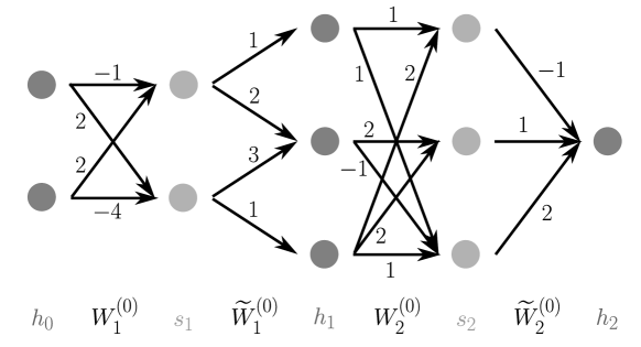
(a) Example of a two-layer augmented neural network $\Phi\in\Xi^{k}_{\textup{A},\mathbb{W}\setminus\mathbb{W}^{\ast}}(\mathcal{X},\mathbb{R})$, where the two weight matrices $W_{1}^{(0)}$ and $W_{2}^{(0)}$ have both not full rank.

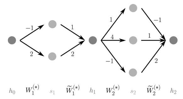
(b) Two-layer neural network $\overline{\Phi}\in\Xi^{k}_{\textup{B},\mathbb{W}^{\ast}}(\mathcal{Y},\mathbb{R})$ with a bottleneck, which has only full rank matrices and which is up to a linear change of coordinates equivalent to the neural network architecture $\Phi$ of 4(a).

Figure 3.4: Equivalent neural network architectures of Example 3.14 to illustrate Theorem 3.12(a).

Theorem 3.12 is an explicit algorithm showing equivalence up to a linear change of coordinates. Due to the linear change of coordinates, it is not guaranteed that the regularity of the critical points of equivalent neural networks stay the same. The following theorem shows that if a coordinate transformation is necessary to obtain an equivalent neural network with full rank matrices, it is possible that degenerate critical points become non-degenerate.

Theorem 3.15.

Let $\Phi\in\Xi^{k}(\mathcal{X},\mathbb{R})$, $k\geq 2$, $\mathcal{X}\subset\mathbb{R}^{n}$ be a classical feed-forward neural network, which is up to the linear change of coordinates $A\in\mathbb{R}^{\bar{n}\times n}$, $\bar{n}\leq n$, $\textup{rank}(A)=\bar{n}$ equivalent to $\overline{\Phi}\in\Xi^{k}(\mathcal{Y},\mathbb{R})$, $\mathcal{Y}=A(\mathcal{X})\subset\mathbb{R}^{\bar{n}}$. Then

$$\overline{\Phi}\in(\mathcal{C}1)^{k}(\mathcal{Y},\mathbb{R})\quad\Leftrightarrow\quad\Phi\in(\mathcal{C}1)^{k}(\mathcal{X},\mathbb{R}).$$

If $\bar{n}=n$, it holds additionally

$$\overline{\Phi}\in(\mathcal{C}2)^{k}(\mathcal{Y},\mathbb{R})\quad \Leftrightarrow\quad\Phi\in(\mathcal{C}2)^{k}(\mathcal{X},\mathbb{R}),$$

$$\overline{\Phi}\in(\mathcal{C}3)^{k}(\mathcal{Y},\mathbb{R})\quad \Leftrightarrow\quad\Phi\in(\mathcal{C}3)^{k}(\mathcal{X},\mathbb{R}).$$

If $\bar{n}<n$, then $\Phi\notin(\mathcal{C}2)^{k}(\mathcal{X},\mathbb{R})$ and it holds

$$\overline{\Phi}\in(\mathcal{C}2)^{k}(\mathcal{X},\mathbb{R})\cup(\mathcal{C}3)^{k}(\mathcal{Y},\mathbb{R})\quad\Leftrightarrow\quad\Phi\in(\mathcal{C}3)^{k}(\mathcal{X},\mathbb{R}).$$

Proof.

As $\Phi\in\Xi^{k}(\mathcal{X},\mathbb{R})$ is up to the linear change of coordinates $A$ equivalent to $\overline{\Phi}\in\Xi^{k}(\mathcal{Y},\mathbb{R})$, it holds

$$\Phi(x)=\overline{\Phi}(Ax)\qquad\text{for all }x\in\mathcal{X}.$$

Calculating the gradient leads to

$$\nabla\Phi(x)=A^{\top}\cdot\nabla\overline{\Phi}(Ax)\qquad\text{for all }x\in\mathcal{X}.$$

If $\nabla\overline{\Phi}(Ax)=0$ for some $x\in\mathcal{X}$ with $y=Ax\in\mathcal{Y}$, then $\nabla\overline{\Phi}(Ax)=0$ for all $x\in\mathcal{X}_{y}$, where

$$\mathcal{X}_{y}\coloneqq\left\{x\in\mathcal{X}:Ax=y\in\mathcal{Y}\right\}.$$

Given $y\in\mathcal{Y}$, $\nabla\overline{\Phi}(y)=0$ implies that $\nabla\Phi(x)=0$ for all $x\in\mathcal{X}_{y}$. As the matrix $A^{\top}\in\mathbb{R}^{n\times\bar{n}}$ has rank $\bar{n}\leq n$, the linear system $A^{\top}\cdot\nabla\overline{\Phi}(y)=0$ has only the solution $\nabla\overline{\Phi}(y)=0$, such that from $\nabla\Phi(x)=0$ for some $x\in\mathcal{X}$ it follows $\nabla\overline{\Phi}(Ax)=0$ for $Ax\in\mathcal{Y}$. Hence, there exists a bijection between the critical points $y\in\mathcal{Y}$ of $\overline{\Phi}$ and the set of critical points $\mathcal{X}_{y}\subset\mathcal{X}$ of $\Phi$. Especially, $\overline{\Phi}$ has critical points if and only if $\Phi$ has critical points, such that the first assertion follows.

To determine the regularity of the critical points, we calculate the Hessian matrices of $\Phi$ and $\overline{\Phi}$:

$$H_{\Phi}(x)=\nabla(\nabla\Phi(x)^{\top})=\nabla(\nabla\overline{\Phi}(Ax)^{\top}\cdot A)=A^{\top}\cdot H_{\overline{\Phi}}(x)\cdot A\qquad\text{for all }x\in\mathcal{X}.$$

As the matrix $A$ has rank $\bar{n}$ and $H_{\overline{\Phi}}(x)$ is a $\bar{n}\times\bar{n}$ matrix, it holds

$$\text{rank}(H_{\Phi}(x))=\text{rank}(A^{\top}\cdot H_{\overline{\Phi}}(x)\cdot A)=\text{rank}(A^{\top}\cdot H_{\overline{\Phi}}(x))=\text{rank}(H_{\overline{\Phi}}(x))\qquad\text{for all }x\in\mathcal{X},$$

which implies with the fact that $H_{\Phi}(x)$ is a $n\times n$ matrix the remaining assertions of the theorem. ∎

The following example shows a neural network with degenerate critical points, which is up to a linear change of coordinate equivalent to a neural network with only non-degenerate critical points. It illustrates the case of Theorem 3.15, where under a linear change of coordinates represented by a full rank matrix $A$, the class of the neural network can change.

Example 3.16.

Consider the neural network $\Phi\in\Xi^{\infty}(\mathbb{R}^{2},\mathbb{R})$ with $L=1$ defined by the weight matrices

$$W_{1}=\begin{pmatrix}1&2\\ 2&4\end{pmatrix},\qquad\widetilde{W}_{1}=\begin{pmatrix}2&-1\end{pmatrix},\qquad b_{1}=\begin{pmatrix}0\\ 0\end{pmatrix},\qquad\tilde{b}_{1}=0,$$

arbitrary biases and soft-plus activation functions $[\sigma_{1}]_{1}(x)=[\sigma_{1}]_{2}(x)=\ln(1+\exp(x))$, see Figure 3.55(a). As $\textup{rank}(W_{1})=1<2$ and $\textup{rank}(\widetilde{W}_{1})=1$, Theorem 3.12(a) implies that there exists a neural network architecture $\overline{\Phi}\in\Xi^{\infty}(\mathbb{R},\mathbb{R})$, which is up to a linear change of coordinates $A:\mathbb{R}^{2}\rightarrow\mathbb{R}$ equivalent to $\Phi$. As $[W_{1}]_{2}=2[W_{1}]_{1}$, it follows by the proof of Theorem 3.12(a) that the weights of $\overline{\Phi}$ and the matrix $A$ are given by

$$\overline{W}_{1}=\begin{pmatrix}1\\ 2\end{pmatrix},\qquad\overline{\widetilde{W}}_{1}=\begin{pmatrix}2&-1\end{pmatrix},\qquad\bar{b}_{1}=\begin{pmatrix}0\\ 0\end{pmatrix},\qquad\bar{\tilde{b}}_{1}=0,\qquad A=\begin{pmatrix}1&2\end{pmatrix},$$

such that $\Phi(x_{1},x_{2})=\overline{\Phi}(x_{1}+2x_{2})=\Phi(y)$ for $y=x_{1}+2x_{2}$. We verify now the properties of Theorem 3.15. It holds

$$\overline{\Phi}(y)=2\ln(1+\exp(y))-\ln(1+\exp(2y))$$

with gradient

$$\nabla\overline{\Phi}(y)=\frac{2\exp(y)(1-\exp(y))}{(1+\exp(y))(1+\exp(2y))},$$

such that $\overline{\Phi}$ has exactly one critical point at $y^{\ast}=0$. The critical point is non-degenerate as

$$H_{\overline{\Phi}}(y^{\ast})=-0.5\neq 0.$$

Consequently $\overline{\Phi}$ is of class $(\mathcal{C}2)^{\infty}(\mathbb{R},\mathbb{R})$. By Theorem 3.15 the original neural network $\Phi$ has to be of class $(\mathcal{C}3)^{\infty}(\mathbb{R}^{2},\mathbb{R})$. It holds

$$\Phi(x_{1},x_{2})=2\ln(1+\exp(x_{1}+2x_{2}))-\ln(1+\exp(2x_{1}+4x_{2})),$$

with gradient

$$\nabla\overline{\Phi}(x_{1},x_{2})=\begin{pmatrix}\frac{2\exp(x_{1}+2x_{2})(1-\exp(x_{1}+2x_{2}))}{(1+\exp(x_{1}+2x_{2}))(1+\exp(2x_{1}+4x_{2}))}\\ \frac{4\exp(x_{1}+2x_{2})(1-\exp(x_{1}+2x_{2}))}{(1+\exp(x_{1}+2x_{2}))(1+\exp(2x_{1}+4x_{2}))}\end{pmatrix},$$

such that $\Phi$ has a line of equilibria defined by $x_{1}+2x_{2}=0$. As the entries of $\nabla\overline{\Phi}(x_{1},x_{2})$ are linearly dependent, the Hessian matrix $H_{\Phi}(x_{1},x_{2})$ is for every $(x_{1},x_{2})\in\mathbb{R}^{2}$ singular, which implies that all equilibria of $\Phi$ are degenerate and $\Phi$ is of class $(\mathcal{C}3)^{\infty}(\mathbb{R}^{2},\mathbb{R})$.

.

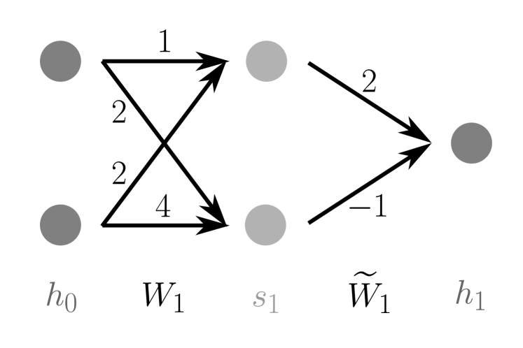
(a) Example of a one-layer neural network $\Phi\in\Xi^{\infty}(\mathbb{R}^{2},\mathbb{R})$ of class $(\mathcal{C}3)^{\infty}(\mathbb{R}^{2},\mathbb{R})$, which has one line of degenerate equilibria.

.

(b) One-layer neural network $\overline{\Phi}\in\Xi^{\infty}(\mathbb{R},\mathbb{R})$ of class $(\mathcal{C}2)^{\infty}(\mathbb{R},\mathbb{R})$, which is up to a linear change of coordinates equivalent to $\Phi$ of 5(a). $\overline{\Phi}$ has one non-degenerate critical point.

.

Figure 3.5: Equivalent neural network architectures of Example 3.16 to illustrate Theorem 3.15.

If we aim to have a large expressivity of classical feed-forward neural networks with respect to the space of $k$ times continuously differentiable functions, Theorem 3.15 implies that we should choose the input dimension as small as possible. If the input dimension $n$ can be reduced, the considered architecture cannot be of class $(\mathcal{C}2)^{k}(\mathcal{X},\mathbb{R})$, so at least one critical point is degenerate. Consequently, the generic class of Morse functions, where every critical point is non-degenerate, cannot be represented.

Due to Lemma 3.6 and Theorems 3.12 and 3.15, we assume in the upcoming analysis, that the considered neural network architecture has only full rank matrices, as every neural network with non-trivial dynamics is up to a linear change of coordinates equivalent to a smaller architecture in normal form and the set of matrices, where at least one weight matrix has not full rank, is a zero set in the weight space.

3.3 Existence of Critical Points

In this section, we study the existence of critical points dependent on the special architecture of the neural network. To that purpose, we first calculate the network gradient.

Lemma 3.17.

Let $\Phi\in\Xi^{k}(\mathcal{X},\mathbb{R})$, $k\geq 1$ be a classical feed-forward neural network with weight matrices $W=(W_{1},\widetilde{W}_{1},\ldots,W_{L},\widetilde{W}_{L})\in\mathbb{W}$ and biases $b=(b_{1},\tilde{b}_{1},\ldots,b_{L},\tilde{b}_{L})\in\mathbb{B}$. Then

$$\nabla\Phi(x)=\left[\widetilde{W}_{L}\Psi_{L}(s_{L})W_{L}\ldots\widetilde{W}_{1}\Psi_{1}(s_{1})W_{1}\right]^{\top}\in\mathbb{R}^{n},$$

where $\Psi_{l}(s_{l})=\textup{diag}([\sigma_{l}]_{i}^{\prime}([s_{l}]_{i}))\in\mathbb{R}^{m_{l}\times m_{l}}$, $i\in\{1,\ldots,m_{l}\}$ is a diagonal matrix.

Proof.

Due to the layer structure of the feed-forward neural network it holds for $l\in\{1,.\ldots,L-1\}$:

$$\Phi(x)=h_{L}=\widetilde{W}_{L}\sigma_{L}(W_{L}(\ldots\sigma_{2}(W_{2}(\widetilde{W}_{1}\sigma_{1}(W_{1}x+b_{1})+\tilde{b}_{1})+b_{2})\ldots)+b_{L})+\tilde{b}_{L}.$$

By Lemma 3.1 it holds $\Phi\in C^{1}(\mathcal{X},\mathbb{R})$, such that the multi-dimensional chain rule implies

$$\frac{\mathrm{d}\Phi}{\mathrm{d}x}=\widetilde{W}_{L}\Psi_{L}(s_{L})W_{L}\ldots\widetilde{W}_{1}\Psi_{1}(s_{1})W_{1}\in\mathbb{R}^{1\times n},$$

where $\Psi_{l}(s_{l})=\textup{diag}([\sigma_{l}]_{i}^{\prime}([s_{l}]_{i}))\in\mathbb{R}^{m_{l}\times m_{l}}$, $i\in\{1,\ldots,m_{l}\}$ is a diagonal matrix. The result follows by taking the transpose. ∎

Due to the reasons established in Section 3.2, we restrict our upcoming analysis to neural networks $\Phi\in\Xi^{k}_{\mathbb{W}^{\ast}}(\mathcal{X},\mathbb{R})$ in normal form. The upcoming theorems established for networks in $\Xi^{k}_{\mathbb{W}^{\ast}}(\mathcal{X},\mathbb{R})$ can be generalized to general networks in $\Xi^{k}(\mathcal{X},\mathbb{R})$ by using the statement of Lemma 3.6, that $\textup{vecm}(\mathbb{W}\setminus\mathbb{W}^{\ast})$ is a zero set in $\mathbb{R}^{N_{W}}$. For non-augmented classical feed-forward neural networks $\Phi$, the following theorem shows, that $\Phi$ has no critical points if all weight matrices have full rank.

Theorem 3.18.

Any non-augmented classical feed-forward neural network $\Phi\in\Xi^{k}_{\textup{N},\mathbb{W}^{\ast}}(\mathcal{X},\mathbb{R})$, $k\geq 1$, with weight matrices $W\in\mathbb{W}^{\ast}$ has no critical point, i.e. $\nabla\Phi(x)\neq 0$ for all $x\in\mathcal{X}$. Consequently it holds for $k\geq 1$

$$\Xi^{k}_{\textup{N},\mathbb{W}^{\ast}}(\mathcal{X},\mathbb{R})\subset(\mathcal{C}1)^{k}(\mathcal{X},\mathbb{R}).$$

This implies that for all weights $(\textup{vecm}(W);\textup{stk}(b))\in\mathbb{R}^{N_{W}+N_{B}}$, $W\in\mathbb{W}$, $b\in\mathbb{B}$ except possibly for a zero set in $\mathbb{R}^{N_{W}+N_{B}}$ w.r.t. the Lebesgue measure, a non-augmented classical feed-forward neural network $\Phi\in\Xi^{k}_{\textup{N}}(\mathcal{X},\mathbb{R})$, $k\geq 1$ is of class $(\mathcal{C}1)^{k}(\mathcal{X},\mathbb{R})$ and hence a Morse function.

Proof.

Let $\Phi\in\Xi^{k}_{N,\mathbb{W}^{\ast}}(\mathcal{X},\mathbb{R})$ with weight matrices $W=(W_{1},\widetilde{W}_{1},\ldots,W_{L},\widetilde{W}_{L})$. By Lemma 3.17 it holds

$$\nabla\Phi(x)=\left[\widetilde{W}_{L}\Psi_{L}(s_{L})W_{L}\ldots\widetilde{W}_{1}\Psi_{1}(s_{1})W_{1}\right]^{\top}\in\mathbb{R}^{n},$$

where $\Psi_{l}(s_{l})=\textup{diag}([\sigma_{l}]_{i}^{\prime}([s_{l}]_{i}))\in\mathbb{R}^{m_{l}\times m_{l}}$, $i\in\{1,\ldots,m_{l}\}$, is a diagonal matrix with $s_{l}=W_{l}h_{l-1}+b_{l}$. As $[\sigma_{l}]_{i}\in C^{k}(\mathbb{R},\mathbb{R})$, $k\geq 1$ is by Definition 3.2 strictly monotone for $l\in\{1,\ldots,L\}$, $i\in\{1,\ldots,m_{l}\}$, it either holds $[\sigma_{l}]_{i}^{\prime}>0$ or $[\sigma_{l}]_{i}^{\prime}<0$. Consequently each matrix $\Psi_{l}(s_{l})$, $l\in\{1,\ldots,L\}$ has non-zero diagonal entries and hence full rank. Due to the assumption $W\in\mathbb{W}^{\ast}$ all matrices $W_{l}$ and $\widetilde{W}_{l}$ have full rank for $l\in\{1,\ldots,L\}$. As the neural network is non-augmented, the dimensions of the full rank matrices $\widetilde{W}_{L},\Psi_{L}(s_{L}),\ldots,\Psi_{1}(s_{1}),W_{1}$ are monotonically increasing, such that Lemma 3.10 implies that the vector $[\nabla\Phi(x)]^{\top}\in\mathbb{R}^{1\times n}$ has independently of $x\in\mathcal{X}$ always rank one. Consequently $\nabla\Phi(x)\neq 0$ for all $x\in\mathcal{X}$. By Definition 2.3 it follows $\Xi^{k}_{\textup{N},\mathbb{W}^{\ast}}(\mathcal{X},\mathbb{R})\subset(\mathcal{C}1)^{k}(\mathcal{X},\mathbb{R})$. The second statement is a consequence of the first part and Lemma 3.6: as $\textup{vecm}(\mathbb{W}\setminus\mathbb{W}^{\ast})$ is a zero set w.r.t. the Lebesgue measure in $\mathbb{R}^{N_{W}}$, it follows that the set of non-full rank matrices and arbitrary biases $\textup{vecm}(\mathbb{W}\setminus\mathbb{W}^{\ast})\times\textup{stk}(\mathbb{B})$ is a zero set in $\mathbb{R}^{N_{W}+N_{B}}$ w.r.t. the Lebesgue measure. ∎

Example 3.19.

Consider the one-layer neural network architecture $\Phi\in\Xi^{k}_{\textup{N}}(\mathbb{R}^{3},\mathbb{R})$, $k\geq 1$ with $L=1$ defined by the weight matrices

$$W_{1}=\begin{pmatrix}w_{11}&w_{12}&w_{13}\\ w_{21}&w_{22}&w_{23}\end{pmatrix}\in\mathbb{R}^{2\times 3},\qquad\widetilde{W}_{1}=(\widetilde{w}_{1},\widetilde{w}_{2})\in\mathbb{R}^{1\times 2},$$

and arbitrary biases, see Figure 3.6. By Lemma 3.17 it holds

$$\nabla\Phi(x) =\begin{pmatrix}w_{11}&w_{21}\\ w_{12}&w_{22}\\ w_{13}&w_{23}\end{pmatrix}\begin{pmatrix}[\sigma_{1}]_{1}^{\prime}([s_{1}]_{1})&0\\ 0&[\sigma_{1}]_{2}^{\prime}([s_{1}]_{2})\end{pmatrix}\begin{pmatrix}\widetilde{w}_{1}\\ \widetilde{w}_{2}\end{pmatrix}$$

$$=\begin{pmatrix}\widetilde{w}_{1}w_{11}[\sigma_{1}]_{1}^{\prime}([s_{1}]_{1})+\widetilde{w}_{2}w_{21}[\sigma_{1}]_{2}^{\prime}([s_{1}]_{2})\\ \widetilde{w}_{1}w_{12}[\sigma_{1}]_{1}^{\prime}([s_{1}]_{1})+\widetilde{w}_{2}w_{22}[\sigma_{1}]_{2}^{\prime}([s_{1}]_{2})\\ \widetilde{w}_{1}w_{13}[\sigma_{1}]_{1}^{\prime}([s_{1}]_{1})+\widetilde{w}_{2}w_{23}[\sigma_{1}]_{2}^{\prime}([s_{1}]_{2})\end{pmatrix}.$$

By Theorem 3.18, there exists no critical point if $W_{1}$ and $\widetilde{W}_{1}$ have both full rank. This is the case, as if $\nabla\Phi(x)=0$ for some $x\in\mathcal{X}$ then

$$\widetilde{w}_{1}[\sigma_{1}]_{1}^{\prime}([s_{1}]_{1})\begin{pmatrix}w_{11}\\ w_{12}\\ w_{13}\end{pmatrix}+\widetilde{w}_{2}[\sigma_{1}]_{2}^{\prime}([s_{1}]_{2})\begin{pmatrix}w_{21}\\ w_{22}\\ w_{23}\end{pmatrix}=\begin{pmatrix}0\\ 0\\ 0\end{pmatrix},$$

such that either $W_{1}$ has only rank 1 as its columns are linearly dependent or the matrix $\widetilde{W}_{1}$ is the zero matrix and has rank 0.

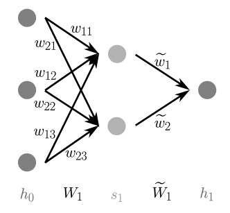
Figure 3.6: One-layer non-augmented neural network architecture $\Phi\in\Xi^{k}_{\textup{N}}(\mathbb{R}^{3},\mathbb{R})$ of Example 3.19.

In contrast to non-augmented neural networks, critical points can exist in the case of augmented or bottleneck architectures. To show this statement in Theorem 3.21, we need the following lemma.

Lemma 3.20.

Given $A\in\mathbb{R}^{1\times n}$, $\textup{rank}(A)=1$ and $C\in\mathbb{R}^{1\times m}$, $\textup{rank}(C)=1$ with $n\leq m$, the linear system $AB=C$ always has a full rank solution $B\in\mathbb{R}^{n\times m}$, $\textup{rank}(B)=n$.

Proof.

As by assumption $\text{rank}(A)=\text{rank}(A|C)=1$, the Rouché-Capelli Theorem [25] guarantees the existence of a solution to the linear system. In the following we show via an explicit construction, that the solution $B$ can be chosen as a full rank matrix. Denote by $\overline{A}=[A]_{i_{1},\ldots,i_{\bar{n}}}\in\mathbb{R}^{1\times\bar{n}}$, $\bar{n}\leq n$, $\{i_{1},\ldots,i_{\bar{n}}\}\subset\{1,\ldots,n\}$ the submatrix of $A$, which consists only of the non-zero entries of $A$, i.e. $[A]_{i_{k}}\neq 0$ for all $k\in\{1,\ldots,\bar{n}\}$ and denote the non-zero entries of $C$ by $[C]_{j_{1},\ldots,j_{\overline{m}}}\in\mathbb{R}^{1\times\overline{m}}$, $\overline{m}\leq m$, i.e. $[C]_{j_{k}}\neq 0$ for all $k\in\{1,\ldots,\overline{m}\}$. If $\overline{m}\geq\bar{n}$, we define the following matrix entries of the submatrix $[B]_{(i_{1},\ldots,i_{\bar{n}}),(1,\ldots,m)}$:

$$[B]_{i_{k},j_{k}} =\frac{[C]_{j_{k}}}{[A]_{i_{k}}}\neq 0,\qquad \text{if }k\in\{1,\ldots,\bar{n}\},$$

$$[B]_{i_{\bar{n}},j_{k}} =\frac{[C]_{j_{k}}}{[A]_{i_{\bar{n}}}}\neq 0,\qquad \text{if }k\in\{\bar{n}+1,\ldots,\overline{m}\},$$

and set all other matrix entries to zero. By construction, $[B]_{(i_{1},\ldots,i_{\bar{n}}),(1,\ldots,m)}$ has rank $\bar{n}$ and it holds

$$\overline{A}\cdot[B]_{(i_{1},\ldots,i_{\bar{n}}),(1,\ldots,m)}=C.$$

If $\overline{m}<\bar{n}$, define $j_{\overline{m}+1},\ldots,j_{\bar{n}}$ to be arbitrary, but different indices of $\{1,\ldots,m\}\setminus\{j_{1},\ldots,j_{\overline{m}}\}$, which is possible as $\bar{n}\leq n\leq m$. Let the matrix entries of $[B]_{(i_{1},\ldots,i_{\bar{n}}),(1,\ldots,m)}$ be

$$[B]_{i_{k},j_{k}} =\frac{[C]_{j_{k}}}{[A]_{i_{k}}}\neq 0,\qquad \text{if }k\in\{1,\ldots,\overline{m}\},$$

$$[B]_{i_{k},j_{k}} =A_{i_{1}},\quad[B]_{i_{1},j_{k}}=-A_{i_{k}},\qquad \text{if }k\in\{\overline{m}+1,\ldots,\bar{n}\},$$

and set all other matrix entries to zero. By construction, $[B]_{(i_{1},\ldots,i_{\bar{n}}),(1,\ldots,m)}$ has rank $\bar{n}$ and it holds

$$\overline{A}\cdot[B]_{(i_{1},\ldots,i_{\bar{n}}),(1,\ldots,m)}=C,$$

as for $k\in\{\overline{m}+1,\ldots,\bar{n}\}$ it holds $\overline{A}\cdot[B]_{(i_{1},\ldots,i_{\bar{n}}),(j_{k})}=A_{i_{1}}A_{i_{k}}-A_{i_{1}}A_{i_{k}}=0=[C]_{j_{k}}$.

For both cases, i.e. $\overline{m}\geq\bar{n}$ and $\overline{m}<\bar{n}$, choose the other rows of $B$, which are not part of $[B]_{(i_{1},\ldots,i_{\bar{n}}),(1,\ldots,m)}$ in such a way, that they are linearly independent of the rows of $[B]_{(i_{1},\ldots,i_{\bar{n}}),(1,\ldots,m)}$. This is possible, as the number $n$ of rows of $B$ is smaller than their dimension $m$. Hence, the constructed matrix $B$ has rank $n$. As $[A]_{i}=0$ for $i\in\{1,\ldots,n\}\setminus\{i_{1},\ldots,i_{\bar{n}}\}$ it follows $AB=C$. ∎

The following proposition shows, that for augmented and bottleneck architectures in normal form, there exist a choice of the full rank matrices $W\in\mathbb{W}^{\ast}$, such that the neural network has a critical point. Hereby the position of the critical point is freely selectable.

Theorem 3.21.

Given $L\geq 1$ and $\mathcal{X}\subset\mathbb{R}^{n}$, for every $x\in\mathcal{X}$ there exist weight matrices $W_{x}\in\mathbb{W}^{\ast}$ corresponding to an augmented architecture $\Phi\in\Xi^{k}_{\textup{A},\mathbb{W}^{\ast}}(\mathcal{X},\mathbb{R})$ and weight matrices $W_{x}\in\mathbb{W}^{\ast}$ corresponding to a bottleneck architecture $\Phi\in\Xi^{k}_{\textup{B},\mathbb{W}^{\ast}}(\mathcal{X},\mathbb{R})$, $k\geq 1$, such that $\nabla\Phi(x)=0$, i.e. $\Phi$ has a critical point at $x\in\mathcal{X}$.

Proof.

For $\Phi\in\Xi^{k}_{\textup{A}}(\mathcal{X},\mathbb{R})$, the first layer of maximal width $g_{l^{\ast}}$, $l^{\ast}\in\{1,\ldots,2L-1\}$ fulfills $d_{l^{\ast}-1}<d_{l^{\ast}}$ and it holds $d_{j-1}\geq d_{j}$ for $l^{\ast}<j\leq 2L$. For $\Phi\in\Xi^{k}_{\textup{B}}(\mathcal{X},\mathbb{R})$, consider the last bottleneck of $\Phi$. Then there exist layers $g_{i}^{\ast}$, $g_{j}^{\ast}$ and $g_{l}^{\ast}$ with $0\leq i^{\ast}<j^{\ast}<l^{\ast}\leq 2L$, such that $d_{i}^{\ast}>d_{j}^{\ast}$, $d_{j}^{\ast}\leq d_{j^{\ast}+1}\leq\ldots\leq d_{l^{\ast}-1}<d_{l}^{\ast}$ and $d_{j-1}\geq d_{j}$ for $l^{\ast}<j\leq 2L$. In both cases there exists a layer $g_{l^{\ast}}$ such that $d_{l^{\ast}-1}<d_{l^{\ast}}$, $d_{l^{\ast}}\geq d_{l^{\ast}+1}$ and from layer $g_{l^{\ast}}$ on-wards the width of the layers is monotonically decreasing.

Let $\Phi\in\Xi^{k}_{\textup{A}}(\mathcal{X},\mathbb{R})\cup\Xi^{k}_{\textup{B}}(\mathcal{X},\mathbb{R})$, fix some $x\in\mathcal{X}$ and denote the weight matrices by $W=(W_{1},\widetilde{W}_{1},\ldots,W_{L},\widetilde{W}_{L})=(V_{1},\ldots,V_{2L})\in\mathbb{W}$, where $V_{1},\ldots,V_{l^{\ast}},V_{l^{\ast}+2},\ldots,V_{2L}$ are arbitrary but fixed full rank matrices. As $d_{l^{\ast}-1}<d_{l^{\ast}}$, the corresponding weight matrix $V_{l^{\ast}}\in\mathbb{R}^{d_{l^{\ast}}\times d_{l^{\ast}-1}}$ has rank $d_{l^{\ast}-1}$, where $V_{l^{\ast}}=\widetilde{W}_{l^{\ast}/2}$ if $l^{\ast}$ is even and $V_{l^{\ast}}=W_{(l^{\ast}+1)/2}$ if $l^{\ast}$ is odd. As $d_{l^{\ast}}>d_{l^{\ast}-1}$ and $\text{rank}(V_{l^{\ast}})=d_{l^{\ast}-1}$, the $d_{l^{\ast}}$ rows of $V_{l^{\ast}}$ are linearly dependent. Hence, there exists a non-trivial linear combination of the rows of $V_{l^{\ast}}$, which results in a zero row, i.e. there exists $v_{l^{\ast}}\in\mathbb{R}^{1\times d_{l^{\ast}}}$, $\text{rank}(v_{l^{\ast}})=1$, such that

$$v_{l^{\ast}}V_{l^{\ast}}=0\in\mathbb{R}^{1\times d_{l^{\ast}-1}}.$$

If $l^{\ast}$ is even, then

$$(\nabla\Phi(x))^{\top}=V_{2L}\Psi_{L}(s_{L})V_{2L-1}\ldots\Psi_{l^{\ast}/2+1}(s_{l^{\ast}/2+1})V_{l^{\ast}+1}V_{l^{\ast}}\ldots V_{2}\Psi_{1}(s_{1})V_{1}\in\mathbb{R}^{1\times n}.$$

As $V_{2L}$, $\Psi_{L}(s_{L})$, …, $\Psi_{l^{\ast}/2+1}(s_{l^{\ast}/2+1})$ are full rank matrices with monotonically increasing width, Lemma  3.10 guarantees that the matrix product $V_{2L}\Psi_{L}(s_{L})\ldots\Psi_{l^{\ast}/2+1}(s_{l^{\ast}/2+1})\in\mathbb{R}^{1\times d_{l^{\ast}+1}}$ has rank one, independently of the choice of $x\in\mathcal{X}$. Since $d_{l^{\ast}}\geq d_{l^{\ast}+1}$, Lemma 3.20 implies that there exist a full rank solution $V_{l^{\ast}+1}\in\mathbb{R}^{d_{l^{\ast}+1}\times d_{l^{\ast}}}$ of the linear system

$$\left[V_{2L}\ldots\Psi_{l^{\ast}/2+1}(s_{l^{\ast}/2+1})\right]V_{l^{\ast}+1}=v_{l^{\ast}}\in\mathbb{R}^{1\times d_{l^{\ast}}}.$$

Hence, there exist weight matrices $W_{x}\in\mathbb{W}^{\ast}$, which depend on $x$, such that $\nabla\Phi(x)=0\in\mathbb{R}^{n}$ for the fixed $x\in\mathcal{X}$. If $l^{\ast}$ is odd, then

$$(\nabla\Phi(x))^{\top}=V_{2L}\Psi_{L}(s_{L})V_{2L-1}\ldots V_{l^{\ast}+2}V_{l^{\ast}+1}\Psi_{(l^{\ast}+1)/2}(s_{(l^{\ast}+1)/2})V_{l^{\ast}}\ldots V_{2}\Psi_{1}(s_{1})V_{1}\in\mathbb{R}^{1\times n}.$$

As $V_{2L}$, …, $V_{l^{\ast}+2}$ are full rank matrices with monotonically increasing width, Lemma  3.10 guarantees that the matrix product $\widetilde{W}_{L}\ldots V_{l^{\ast}+2}\in\mathbb{R}^{1\times d_{l^{\ast}+1}}$ has rank one, independently of the choice of $x\in\mathcal{X}$. As $\Psi_{(l^{\ast}+1)/2}(s_{(l^{\ast}+1)/2})$ is a diagonal, invertible full rank matrix, $v_{l^{\ast}}\left[\Psi_{(l^{\ast}+1)/2}(s_{(l^{\ast}+1)/2})\right]^{-1}$ has rank one. Since $d_{l^{\ast}}\geq d_{l^{\ast}+1}$, Lemma 3.20 implies that there exist a full rank solution $V_{l^{\ast}+1}\in\mathbb{R}^{d_{l^{\ast}+1}\times d_{l^{\ast}}}$ of the linear system

$$\left[V_{2L}\ldots V_{l^{\ast}+2}\right]V_{l^{\ast}+1}=v_{l^{\ast}}\left[\Psi_{(l^{\ast}+1)/2}(s_{(l^{\ast}+1)/2})\right]^{-1}\in\mathbb{R}^{1\times d_{l^{\ast}}}.$$

Hence there exist weight matrices $W_{x}\in\mathbb{W}^{\ast}$, which depend on $x$, such that $\nabla\Phi(x)=0\in\mathbb{R}^{n}$ for the fixed $x\in\mathcal{X}$. As $\Phi$ was an augmented or a bottleneck neural network, the result holds for both architectures. ∎

Examples of augmented and bottleneck architectures, which have critical points are shown in Examples 3.27 and 3.29, when the regularity of the critical points is analyzed. The last theorem has shown, that for every $x\in\mathcal{X}$, the weight matrices of augmented neural networks and neural networks with a bottleneck can be chosen in such a way, that $x\in\mathcal{X}$ is a critical point. From this statement we cannot deduce if it is a generic property of augmented and bottleneck architectures to have a critical point or not. In the following we show, that if there exists for a fixed architecture a non-degenerate critical point, then the set of weights, such that the corresponding neural network has a non-degenerate critical point, has non-zero Lebesgue measure in the weight space. Hence, if for one set of weights, a non-degenerate critical point exist, it is locally a generic property of the chosen architecture to have at least one non-degenerate critical point.

Theorem 3.22.

Let $\Phi\in\Xi^{k}(\mathcal{X},\mathbb{R})$, $k\geq 2$ be a classical feed-forward neural network with weight matrices $W^{\ast}\in\mathbb{W}$. If $\Phi$ has a non-degenerate critical point $x^{\ast}\in\mathcal{X}$, then there exist an open neighborhood $\mathcal{V}$ of $w^{\ast}=\textup{vecm}(W^{\ast})\in\mathbb{R}^{N_{W}}$, which has non-zero Lebesgue measure in $\mathbb{R}^{N_{W}}$, such that for every $w\in\mathcal{V}$, the corresponding neural network has at least one critical point. By choosing $\mathcal{V}$ small enough, it can be guaranteed that at last one critical point of the corresponding neural network is non-degenerate.

Proof.

Let $w^{\ast}=\textup{vecm}(W^{\ast})\in\mathbb{R}^{N_{W}}$ be the vector of stacked weight matrices of the neural network $\Phi$. Define the function

$$F:\mathcal{X}\times\mathbb{R}^{N_{W}}\rightarrow\mathbb{R}^{n},\qquad(x,w)\mapsto F(x,w)=\nabla\Phi(x)$$

with $\mathcal{X}\subset\mathbb{R}^{n}$ open and $\nabla\Phi(x)$ defined in Lemma 3.17, which also depends on $w\in\mathbb{R}^{N_{W}}$. As $k\geq 2$, $\Phi$ is a composition of functions, which are at least twice differentiable in $x$ and $w$, such that $F$ is a continuously differentiable function. By assumption, the neural network $\Phi$ has a critical point at $x^{\ast}\in\mathcal{X}$, such that $F(x^{\ast},w^{\ast})=0$. The $n\times n$ matrix

$$\frac{\partial F}{\partial x}=\frac{\nabla\Phi(x)}{\partial x}=H_{\Phi}(x)$$

is non-singular at the point $(x^{\ast},w^{\ast})$ as by assumption $x^{\ast}$ is a non-degenerate critical point. The Implicit Function Theorem (cf. [6]) now implies that there exist open neighborhoods $\mathcal{U}\subset\mathcal{X}$ and $\mathcal{V}\subset\mathbb{R}^{N_{W}}$ with $(x^{\ast},w^{\ast})\in\mathcal{U}\times\mathcal{V}$ and a continuously differentiable function $g:\mathcal{V}\rightarrow\mathcal{U}$ with $g(w^{\ast})=x^{\ast}$ such that

$$F(g(w),w)=0\qquad\text{for all }w\in\mathcal{V}.$$

Consequently for every $w\in\mathcal{V}$, the corresponding neural network has a critical point at $x=g(w)$. As $\mathcal{V}$ is an open set in $\mathbb{R}^{N_{W}}$ it has non-zero Lebesgue measure. As the determinant of the matrix $\frac{\partial F}{\partial x}=H_{\Phi}(x)$ is a continuous function in $w$, the neighborhood $\mathcal{V}$ can be chosen small enough, such that the critical point $x=g(w)$ is for every $w\in\mathcal{V}$ non-degenerate. ∎

3.4 Regularity of Critical Points

To prove the main results of this section, we use the following lemma of differential geometry, characterizing Morse function not via their Hessian, but via the mixed second derivatives with respect to the weights and the input data.

Lemma 3.23 ([20]).

Let $\widehat{\Lambda}\in C^{2}(\mathcal{X}\times\mathcal{V},\mathbb{R})$, $\mathcal{X}\subset\mathbb{R}^{n}$, $\mathcal{V}\subset\mathbb{R}^{p}$ with $n\leq p$ and denote by $\Lambda_{v}\in C^{2}(\mathcal{X},\mathbb{R})$ the family of functions $\Lambda_{v}(x)\coloneqq\widehat{\Lambda}(x,v)$, which depend continuously on the parameter $v\in\mathcal{V}$. If

$$\frac{\partial^{2}\widehat{\Lambda}}{\partial v\partial x}(x,v)\in\mathbb{R}^{n\times p},\quad\left[\frac{\partial^{2}\widehat{\Lambda}}{\partial v\partial x}(x,v)\right]_{ij}=\frac{\partial^{2}\widehat{\Lambda}}{\partial v_{j}\partial x_{i}}(x,v),\quad i\in\{1,\ldots,n\},\;j\in\{1,\ldots,p\},$$

is for every $(x,v)\in\mathcal{X}\times\mathcal{V}$ surjective, i.e. the matrix $\frac{\partial^{2}\widehat{\Lambda}}{\partial v\partial x}(x,v)$ has for every $(x,v)\in\mathcal{X}\times\mathcal{V}$ full rank $n$, then there exists a set $\mathcal{V}_{0}\subset\mathcal{V}$ of Lebesgue measure zero in $\mathbb{R}^{p}$, such that the function $\Lambda_{v}$ is for all weights $v\in\mathcal{V}\setminus\mathcal{V}_{0}$ a Morse function.

Example 3.24.

Let $\widehat{\Lambda}\in C^{2}(\mathbb{R}\times\mathbb{R}^{2},\mathbb{R})$ be defined by $\widehat{\Lambda}(x,v_{1},v_{2})=v_{1}x^{2}+v_{2}x$. As the matrix

$$\frac{\partial^{2}\widehat{\Lambda}}{\partial v\partial x}(x,v)=\left(2x,1\right)$$

has for all $(x,v)\in\mathbb{R}\times\mathbb{R}^{2}$ rank one, Lemma 3.23 implies that $\Lambda_{v}(x)=v_{1}x^{2}+v_{2}x$ is for all $v\in\mathbb{R}^{2}$, except possibly for a set $\mathcal{V}_{0}\subset\mathbb{R}$ of Lebesgue measure zero, a Morse function. In this example $\mathcal{V}_{0}=(0,0)$ as for $v_{1}\neq 0$ it holds for the Hessian $H_{\Lambda_{v}}(x)=2v_{1}\neq 0$, such that every possible critical point is non-degenerate. For $v_{1}=0$ and $v_{2}\neq 0$, the map $\Lambda_{v}$ has no critical point and hence is a Morse function, only for $v_{1}=v_{2}=0$ the map $\Lambda_{v}$ has degenerate critical points and is no Morse function.

The idea to apply Theorem 3.23 to feed-forward neural networks was already used b¡ Kurochkin in [16]. In this work, we rigorously proof an analogous result to the main theorem of [16] for our more general setting.

Theorem 3.25.

Any augmented classical feed-forward neural network $\Phi\in\Xi^{k}_{\textup{A}}(\mathcal{X},\mathbb{R})$, $k\geq 2$, with weight matrices $W\in\mathbb{W}^{\ast}$ and biases $b\in\mathbb{B}$, is for all weights $(\textup{vecm}(W);\textup{stk}(B))\in\mathbb{R}^{N_{W}+N_{B}}$, except possibly for a zero set in $\mathbb{R}^{N_{W}+N_{B}}$ w.r.t. the Lebesgue measure, of class $(\mathcal{C}1)^{k}(\mathcal{X},\mathbb{R})$ or $(\mathcal{C}2)^{k}(\mathcal{X},\mathbb{R})$ and hence a Morse function. The same statement holds if $\mathbb{W}^{\ast}$ is replaced by $\mathbb{W}$.

Proof.

Let $\Phi\in\Xi^{k}_{\textup{A},\mathbb{W}^{\ast}}(\mathcal{X},\mathbb{R})$, $k\geq 2$ be an augmented classical feed-forward neural network with weight matrices $(W_{1},\widetilde{W}_{1},\ldots,W_{L},\widetilde{W}_{L})\in\mathbb{W}^{\ast}$. By Theorem 3.21 it is possible that the neural network $\Phi$ has a critical point. In the case that $\Phi$ has no critical point, $\Phi$ is of class $(\mathcal{C}1)^{k}(\mathcal{X},\mathbb{R})$ and hence a Morse function. In the following we show that if $\Phi$ has a critical point, then it is for all weights, where $\Phi$ has critical points, except possibly for a zero set w.r.t. the Lebesgue measure, of class $(\mathcal{C}2)^{k}(\mathcal{X},\mathbb{R})$. To show this statement, we consider feed-forward neural networks with full rank weight matrices $W=(W_{1},\widetilde{W}_{1},\ldots,W_{L},\widetilde{W}_{L})\in\mathbb{W}^{\ast}$. By Lemma 3.17, the gradient of $\Phi$ is given by

$$\nabla\Phi(x)=\left[\widetilde{W}_{L}\Psi_{L}(s_{L})W_{L}\ldots\widetilde{W}_{1}\Psi_{1}(s_{1})W_{1}\right]^{\top}\in\mathbb{R}^{n},$$

where $\Psi_{l}(s_{l})=\textup{diag}([\sigma_{l}]_{i}^{\prime}([s_{l}]_{i}))\in\mathbb{R}^{n_{l}\times n_{l}}$, $i\in\{1,\ldots,n_{l}\}$, is a diagonal matrix with $s_{l}=W_{l}h_{l-1}+b_{l}$, $W\in\mathbb{W}^{\ast}$ and $b\in\mathbb{B}$. Let $v=(\textup{vecm}(W);\textup{stk}(b))\in\mathbb{R}^{p}$ with $p=N_{W}+N_{B}$ be the vector with all stacked weight matrices and biases and define $\widehat{\Phi}\in C^{k}(\mathcal{X}\times\left(\textup{vecm}(\mathbb{W}^{\ast})\times\textup{stk}(\mathbb{B})\right))$, $k\geq 2$ to be the neural network $\Phi$ with an explicit dependence on the weight vector $v\in\textup{vecm}(\mathbb{W}^{\ast})\times\textup{stk}(\mathbb{B})$. As a composition of $k$ times continuously differentiable functions $\widehat{\Phi}$ is not only in $x$ but also in $v$ $k$ times continuously differentiable. The second partial derivatives $\frac{\partial^{2}\widehat{\Phi}}{\partial v\partial x}\in\mathbb{R}^{n\times p}$ of $\widehat{\Phi}$ w.r.t. $x$ and $v$ can be explicitly calculated. First we calculate the derivatives w.r.t. the components of the biases $[b_{l}]_{i}$, $l\in\{1,\ldots,L\}$, $i\in\{1,\ldots,m_{l}\}$. They are given by

$$\frac{\partial^{2}\widehat{\Phi}}{\partial[b_{l}]_{i}\partial x}=\; \frac{\partial}{\partial[b_{l}]_{i}}\left[W_{1}^{\top}\Psi_{1}(s_{1})\widetilde{W}_{1}^{\top}\ldots W_{L}^{\top}\Psi_{L}(s_{L})\widetilde{W}_{L}^{\top}\right]$$

$$=\; \sum_{k=l}^{L}W_{1}^{\top}\Psi_{1}(s_{1})\ldots W_{k}^{\top}\Psi_{k}^{\prime}(s_{k})\textup{ diag}\left(\left[\frac{\partial s_{k}}{\partial[b_{l}]_{i}}\right]\right)\widetilde{W}_{k}^{\top}W_{k+1}^{\top}\ldots\Psi_{L}(s_{L})\widetilde{W}_{L}^{\top}$$

$$=\; \sum_{k=l}^{L}W_{1}^{\top}\ldots\Psi_{k}^{\prime}(s_{k})\textup{ diag}\left(\left[W_{k}\widetilde{W}_{k-1}\Psi_{k-1}(s_{k-1})\ldots\Psi_{l}(s_{l})\mathrm{e}_{i}^{(m_{l})}\right]\right)\widetilde{W}_{k}^{\top}\ldots\widetilde{W}_{L}^{\top},$$

where $\Psi_{k}^{\prime}(s_{k})=\textup{diag}([\sigma_{k}]_{i}^{\prime\prime}([s_{k}]_{i}))\in\mathbb{R}^{m_{k}\times m_{k}}$, $i\in\{1,\ldots,m_{k}\}$ and $\frac{\partial s_{k}}{\partial[b_{l}]_{i}}\in\mathbb{R}^{m_{k}}$, $k\in\{l,\ldots,L\}$. The operator diag applied to a vector $y\in\mathbb{R}^{m_{k}}$ defines a diagonal matrix in $\mathbb{R}^{m_{k}\times m_{k}}$ with the entries $y$ component-wise on its diagonal. The vector $\mathrm{e}_{i}^{(m_{l})}$ denotes the $i$-th unit vector in $\mathbb{R}^{m_{l}}$. In the calculation the product rule and the multidimensional chain rule was used. Analogously it follows for the biases $[\tilde{b}_{l}]_{i}$, $l\in\{1,\ldots,L-1\}$, $i\in\{1,\ldots,n_{l}\}$ that

$$\frac{\partial^{2}\widehat{\Phi}}{\partial[\tilde{b}_{l}]_{i}\partial x}=\; \frac{\partial}{\partial[\tilde{b}_{l}]_{i}}\left[W_{1}^{\top}\Psi_{1}(s_{1})\widetilde{W}_{1}^{\top}\ldots W_{L}^{\top}\Psi_{L}(s_{L})\widetilde{W}_{L}^{\top}\right]$$

$$=\; \sum_{k=l+1}^{L}W_{1}^{\top}\Psi_{1}(s_{1})\ldots W_{k}^{\top}\Psi_{k}^{\prime}(s_{k})\textup{ diag}\left(\left[\frac{\partial s_{k}}{\partial[\tilde{b}_{l}]_{i}}\right]\right)\widetilde{W}_{k}^{\top}W_{k+1}^{\top}\ldots\Psi_{L}(s_{L})\widetilde{W}_{L}^{\top}$$

$$=\; \sum_{k=l+1}^{L}W_{1}^{\top}\ldots\Psi_{k}^{\prime}(s_{k})\textup{ diag}\left(\left[W_{k}\widetilde{W}_{k-1}\Psi_{k-1}(s_{k-1})\ldots W_{l+1}\mathrm{e}_{i}^{(n_{l})}\right]\right)\widetilde{W}_{k}^{\top}\ldots\widetilde{W}_{L}^{\top}$$

and

$$\frac{\partial^{2}\widehat{\Phi}}{\partial\tilde{b}_{L}\partial x}=\frac{\partial}{\partial\tilde{b}_{L}}\left[W_{1}^{\top}\Psi_{1}(s_{1})\widetilde{W}_{1}^{\top}\ldots W_{L}^{\top}\Psi_{L}(s_{L})\widetilde{W}_{L}^{\top}\right]=0$$

where $\tilde{b}_{L}\in\mathbb{R}$.

The derivatives w.r.t. the matrix entries $[W_{l}]_{ij}$, $l\in\{1,\ldots,L\}$, $i\in\{1,\ldots,m_{l}\}$, $j\in\{1,\ldots,n_{l-1}\}$ are given by

$$\frac{\partial^{2}\widehat{\Phi}}{\partial[W_{l}]_{ij}\partial x}=\; \frac{\partial}{\partial[W_{l}]_{ij}}\left[W_{1}^{\top}\Psi_{1}(s_{1})\widetilde{W}_{1}^{\top}\ldots W_{L}^{\top}\Psi_{L}(s_{L})\widetilde{W}_{L}^{\top}\right]$$

$$=\; \sum_{k=l}^{L}W_{1}^{\top}\Psi_{1}(s_{1})\ldots W_{k}^{\top}\Psi_{k}^{\prime}(s_{k})\textup{ diag}\left(\left[\frac{\partial s_{k}}{\partial[W_{l}]_{ij}}\right]\right)\widetilde{W}_{k}^{\top}W_{k+1}^{\top}\ldots\Psi_{L}(s_{L})\widetilde{W}_{L}^{\top}$$

$$+W_{1}^{\top}\Psi_{1}(s_{1})\ldots\Psi_{l-1}(s_{l-1})\widetilde{W}_{l-1}^{\top}\delta_{ij}^{n_{l-1}\times m_{l}}\Psi_{l}(s_{l})\ldots\Psi_{L}(s_{L})\widetilde{W}_{L}^{\top}$$

$$=\; \sum_{k=l}^{L}W_{1}^{\top}\ldots\Psi_{k}^{\prime}(s_{k})\textup{ diag}\left(\left[W_{k}\widetilde{W}_{k-1}\Psi_{k-1}(s_{k-1})\ldots\Psi_{l}(s_{l})\mathrm{e}_{i}^{(m_{l})}[h_{l}]_{j}\right]\right)\widetilde{W}_{k}^{\top}\ldots\widetilde{W}_{L}^{\top}$$

$$+W_{1}^{\top}\Psi_{1}(s_{1})\ldots\Psi_{l-1}(s_{l-1})\widetilde{W}_{l-1}^{\top}\delta_{ij}^{n_{l-1}\times m_{l}}\Psi_{l}(s_{l})\ldots\Psi_{L}(s_{L})\widetilde{W}_{L}^{\top}$$

where $\delta_{ij}^{n_{l-1}\times m_{l}}$ denotes the matrix in $\mathbb{R}^{n_{l-1}\times m_{l}}$, which has everywhere zeros, only at the $i,j$-th entry the number one. Analogously it follows for the weight matrices $[\widetilde{W}_{l}]_{ij}$, $l\in\{1,\ldots,L-1\}$, $i\in\{1,\ldots,n_{l}\}$, $j\in\{1,\ldots,m_{l}\}$ that

$$\frac{\partial^{2}\widehat{\Phi}}{\partial[\widetilde{W}_{l}]_{ij}\partial x}=\; \frac{\partial}{\partial[\widetilde{W}_{l}]_{ij}}\left[W_{1}^{\top}\Psi_{1}(s_{1})\widetilde{W}_{1}^{\top}\ldots W_{L}^{\top}\Psi_{L}(s_{L})\widetilde{W}_{L}^{\top}\right]$$

$$=\; \sum_{k=l+1}^{L}W_{1}^{\top}\Psi_{1}(s_{1})\ldots W_{k}^{\top}\Psi_{k}^{\prime}(s_{k})\textup{ diag}\left(\left[\frac{\partial s_{k}}{\partial[\widetilde{W}_{l}]_{ij}}\right]\right)\widetilde{W}_{k}^{\top}W_{k+1}^{\top}\ldots\Psi_{L}(s_{L})\widetilde{W}_{L}^{\top}$$

$$+W_{1}^{\top}\Psi_{1}(s_{1})\ldots\Psi_{l}(s_{l})\delta_{ij}^{m_{l}\times n_{l}}W_{l+1}^{\top}\Psi_{l+1}(s_{l+1})\ldots\Psi_{L}(s_{L})\widetilde{W}_{L}^{\top}$$

$$=\; \sum_{k=l+1}^{L}W_{1}^{\top}\ldots\Psi_{k}^{\prime}(s_{k})\textup{ diag}\left(\left[W_{k}\widetilde{W}_{k-1}\Psi_{k-1}(s_{k-1})\ldots W_{l+1}\mathrm{e}_{i}^{(n_{l})}[\sigma_{l}(s_{l})]_{j}\right]\right)\widetilde{W}_{k}^{\top}\ldots\widetilde{W}_{L}^{\top}$$

$$+W_{1}^{\top}\Psi_{1}(s_{1})\ldots\Psi_{l}(s_{l})\delta_{ij}^{m_{l}\times n_{l}}W_{l+1}^{\top}\Psi_{l+1}(s_{l+1})\ldots\Psi_{L}(s_{L})\widetilde{W}_{L}^{\top}$$

and

$$\frac{\partial^{2}\widehat{\Phi}}{\partial[\widetilde{W}_{L}]_{1j}\partial x}=W_{1}^{\top}\Psi_{1}(s_{1})\widetilde{W}_{1}^{\top}\ldots W_{L}^{\top}\Psi_{L}(s_{L})\delta_{1j}^{m_{l}\times 1}$$

for $j\in\{1,\ldots,m_{L}\}$ as $\widetilde{W}_{L}\in\mathbb{R}^{1\times m_{L}}$. All calculated derivatives are columns of the matrix $\frac{\partial^{2}\widehat{\Phi}}{\partial v\partial x}\in\mathbb{R}^{n\times p}$. To apply Lemma 3.23 we show that the matrix $\frac{\partial^{2}\widehat{\Phi}}{\partial v\partial x}\in\mathbb{R}^{n\times p}$ has at any point $(x,v)\in\mathcal{X}\times\left(\textup{vecm}(\mathbb{W}^{\ast})\times\textup{stk}(\mathbb{B})\right)$ full rank, i.e. rank $n$ as $n\leq p$. As elementary column operations do not change the rank of a matrix, we can subtract for fixed $l\in\{1,\ldots,L\}$ from the columns $\frac{\partial^{2}\widehat{\Phi}}{\partial[W_{l}]_{ij}\partial x}$, $i\in\{1,\ldots,m_{l}\}$, $j\in\{1,\ldots,n_{l-1}\}$, corresponding to the weight matrix $W_{l}$, the columns $\frac{\partial^{2}\widehat{\Phi}}{\partial[b_{l}]_{i}\partial x}$, $i\in\{1,\ldots,m_{l}\}$, corresponding to the bias $b_{l}$, each multiplied with $[h_{l}]_{j}$, $j\in\{1,\ldots,n_{l-1}\}$. We obtain

$$\frac{\partial^{2}\widehat{\Phi}}{\partial[W_{l}]_{ij}\partial x}-\frac{\partial^{2}\widehat{\Phi}}{\partial[b_{l}]_{i}\partial x}\cdot[h_{l}]_{j}=W_{1}^{\top}\Psi_{1}(s_{1})\ldots\Psi_{l-1}(s_{l-1})\widetilde{W}_{l-1}^{\top}\delta_{ij}^{n_{l-1}\times m_{l}}\Psi_{l}(s_{l})\ldots\Psi_{L}(s_{L})\widetilde{W}_{L}^{\top}.$$ (3.2)

Analogously we can without changing the rank of the matrix subtract for fixed $l\in\{1,\ldots,L\}$ from the columns $\frac{\partial^{2}\widehat{\Phi}}{\partial[\widetilde{W}_{l}]_{ij}\partial x}$, $i\in\{1,\ldots,n_{l}\}$, $j\in\{1,\ldots,m_{l}\}$, corresponding to the weight matrix $\widetilde{W}_{l}$, the columns $\frac{\partial^{2}\widehat{\Phi}}{\partial[\tilde{b}_{l}]_{i}\partial x}$, $i\in\{1,\ldots,n_{l}\}$, corresponding to the bias $\tilde{b}_{l}$, each multiplied with every $[\sigma_{l}(s_{l})]_{j}$, $j\in\{1,\ldots,m_{l}\}$. We obtain

$$\frac{\partial^{2}\widehat{\Phi}}{\partial[\widetilde{W}_{l}]_{ij}\partial x}-\frac{\partial^{2}\widehat{\Phi}}{\partial[\tilde{b}_{l}]_{i}\partial x}\cdot[\sigma_{l}(s_{l})]_{j}=W_{1}^{\top}\Psi_{1}(s_{1})\ldots\Psi_{l}(s_{l})\delta_{ij}^{m_{l}\times n_{l}}W_{l+1}^{\top}\Psi_{l+1}(s_{l+1})\ldots\Psi_{L}(s_{L})\widetilde{W}_{L}^{\top}.$$ (3.3)

As the neural network $\Phi$ is augmented, there exists a layer $g_{l^{\ast}}$ of maximal width, $l^{\ast}\in\{1,\ldots,2L-1\}$, which has at least $n+1$ nodes, i.e. $d_{l^{\ast}}\geq n+1$. If $l^{\ast}$ is even, the layer $g_{l^{\ast}}$ of maximal width corresponds to the layer $h_{l^{\ast}/2}$, and we consider the modified columns (3.2) for the index $l^{\ast}/2+1$. We obtain

$$\;\frac{\partial^{2}\widehat{\Phi}}{\partial[W_{l^{\ast}/2+1}]_{ij}\partial x}-\frac{\partial^{2}\widehat{\Phi}}{\partial[b_{l^{\ast}/2+1}]_{i}\partial x}\cdot[h_{l^{\ast}/2+1}]_{j}$$

$$=\, \;W_{1}^{\top}\ldots\widetilde{W}_{l^{\ast}/2}^{\top}\delta_{ij}^{n_{l^{\ast}/2}\times m_{l^{\ast}/2+1}}\Psi_{l^{\ast}/2+1}(s_{l^{\ast}/2+1})\ldots\widetilde{W}_{L}^{\top}$$ (3.4)

$$\eqqcolon \;Y\delta_{ij}^{n_{l^{\ast}/2}\times{m_{l^{\ast}/2+1}}}Z$$

$$= \;Y_{i}\cdot[Z]_{j}\in\mathbb{R}^{n},$$ (3.5)

where $Y=[Y_{1},\ldots,Y_{n_{l^{\ast}/2}}]\in\mathbb{R}^{n\times n_{l^{\ast}/2}}$ and $Z\in\mathbb{R}^{m_{l^{\ast}/2+1}}$ are implicitly defined by equation (3.4). Expression (3.5) follows from the simple structure of the matrix $\delta_{ij}^{n_{l^{\ast}/2}\times m_{l^{\ast}/2+1}}$: it holds

$$Y\delta_{ij}^{n_{l^{\ast}/2}\times m_{l^{\ast}/2+1}}Z=Y\mathrm{e}_{i}^{(n_{l^{\ast}/2})}[Z]_{j}=Y_{i}\cdot[Z]_{j},$$

where $\mathrm{e}_{i}^{(n_{l^{\ast}/2})}$ denotes the $i$-th unit vector in $\mathbb{R}^{n_{l^{\ast}/2}}$ and $[Z]_{j}$ the $j$-th component of the vector $Z$. If $l^{\ast}$ is odd, the layer $g_{l^{\ast}}$ of maximal width corresponds to the layer $s_{(l^{\ast}+1)/2}$, and we consider the modified columns (3.2) for the index $(l^{\ast}+1)/2$. Analogously we obtain

$$\frac{\partial^{2}\widehat{\Phi}}{\partial[\widetilde{W}_{(l^{\ast}+1)/2}]_{ij}\partial x}-\frac{\partial^{2}\widehat{\Phi}}{\partial[\tilde{b}_{(l^{\ast}+1)/2}]_{i}\partial x}\cdot[\sigma_{(l^{\ast}+1)/2}(s_{(l^{\ast}+1)/2})]_{j}$$

$$=\, \;W_{1}^{\top}\ldots\Psi_{(l^{\ast}+1)/2}(s_{(l^{\ast}+1)/2})\delta_{ij}^{m_{(l^{\ast}+1)/2}\times n_{(l^{\ast}+1)/2}}W_{(l^{\ast}+3)/2}^{\top}\ldots\widetilde{W}_{L}^{\top}$$ (3.6)

$$\eqqcolon \;\widetilde{Y}\delta_{ij}^{m_{(l^{\ast}+1)/2}\times n_{(l^{\ast}+1)/2}}\widetilde{Z}$$

$$= \;\widetilde{Y}_{i}\cdot[\widetilde{Z}]_{j}\in\mathbb{R}^{n},$$ (3.7)

where $\widetilde{Y}=[\widetilde{Y}_{1},\ldots,\widetilde{Y}_{m_{(l^{\ast}+1)/2}}]\in\mathbb{R}^{n\times m_{(l^{\ast}+1)/2}}$ and $\widetilde{Z}\in\mathbb{R}^{n_{(l^{\ast}+1)/2}}$ are implicitly defined by equation (3.6). If $(l^{\ast}+1)/2=L$, the matrix product $\widetilde{Z}$ does not exist, so we define $\widetilde{Z}=1\in\mathbb{R}^{n_{L}}=\mathbb{R}$. In both cases we obtain from equations (3.5) or (3.7) modified columns of the form

$$\overline{Y}_{i}[\overline{Z}]_{j}\in\mathbb{R}^{n},\qquad i\in\{1,\ldots,d_{l^{\ast}}\},j\in\{1,\ldots,d_{l^{\ast}+1}\}$$

with $\overline{Y}=[\overline{Y}_{1},\ldots,\overline{Y}_{d_{l^{\ast}}}]\in\mathbb{R}^{n\times d_{l^{\ast}}}$ and $\overline{Z}\in\mathbb{R}^{d_{l^{\ast}+1}}$., where $d_{l}^{\ast}\geq n+1$ is the number of nodes in the layer of maximal width $g_{l^{\ast}}$.

In the following we aim to show that for every $(x,v)\in\mathcal{X}\times\left(\textup{vecm}(\mathbb{W}^{\ast})\times\textup{stk}(\mathbb{B})\right)$, there exists an index $j\in\{1,\ldots,d_{l^{\ast}+1}\}$, such that the matrix

$$Q_{j}\coloneqq\left[\overline{Y}_{1}\cdot[\overline{Z}]_{j},\ldots,\overline{Y}_{d_{l^{\ast}}}\cdot[\overline{Z}]_{j}\right]\in\mathbb{R}^{n\times d_{l^{\ast}}}$$ (3.8)

has full rank $n$. As $Q_{j}$ is a submatrix of $\frac{\partial^{2}\widehat{\Phi}}{\partial v\partial x}\in\mathbb{R}^{n\times p}$ of rank $n$, also the matrix $\frac{\partial^{2}\widehat{\Phi}}{\partial v\partial x}$ has full rank $n$ for every $(x,v)\in\mathcal{X}\times\left(\textup{vecm}(\mathbb{W}^{\ast})\times\textup{stk}(\mathbb{B})\right)$. Due to the assumption $(W_{1},\widetilde{W}_{1},\ldots,W_{L},\widetilde{W}_{L})\in\mathbb{W}^{\ast}$ all considered weight matrices as well as the diagonal matrices $\Psi_{l}(s_{l})$, $l\in\{1,\ldots,L\}$ have full rank. Since the neural network $\Phi$ is augmented, it holds $d_{i}\leq d_{j}$ for $0\leq i<j\leq l^{\ast}$ and $d_{i}\geq d_{j}$ for $l^{\ast}\leq i<j\leq L$. By Lemma 3.10, also the matrix products $\overline{Y}$ and $\overline{Z}$ have full rank, i.e. $\textup{rank}(\overline{Y})=n$ and $\textup{rank}(\overline{Z})=1$ (this also holds in the special case where $\overline{Z}=1$ for $(l^{\ast}+1)/2=L$). Consequently the vector $\overline{Z}\in\mathbb{R}^{d_{l^{\ast}+1}}$ has at least one non-zero entry, i.e. $[\overline{Z}]_{j^{\ast}}\neq 0$ for some $j^{\ast}\in\{1,\ldots,d_{l^{\ast}+1}\}$. As $\overline{Z}$ depends on $(x,v)\in\mathcal{X}\times\left(\textup{vecm}(\mathbb{W}^{\ast})\times\textup{stk}(\mathbb{B})\right)$, also the choice of $j^{\ast}$ depends on $x$ and $v$. For the index $j^{\ast}$, the matrix $Q_{j^{\ast}}$ arises from the matrix $\overline{Y}$ by elementary column operations, as each column is multiplied by the non-zero scalar $[Z]_{j^{\ast}}$. As the matrix $\overline{Y}$ has full rank $n$, also the matrix $Q_{j^{\ast}}$ has full rank $n$, which implies that $\frac{\partial^{2}\widehat{\Phi}}{\partial v\partial x}$ has full rank $n$ for every $(x,v)\in\mathcal{X}\times\left(\textup{vecm}(\mathbb{W}^{\ast})\times\textup{stk}(\mathbb{B})\right)$. As the map $\widehat{\Phi}\in C^{k}\left(\mathcal{X}\times\left(\textup{vecm}(\mathbb{W}^{\ast})\times\textup{stk}(\mathbb{B})\right)\right)$, $k\geq 2$, fulfills the assumptions of Lemma 3.23, it follows that for all weights $v\in\mathcal{V}\coloneqq\textup{vecm}(\mathbb{W}^{\ast})\times\textup{stk}(\mathbb{B})$, except possibly for a zero set $\mathcal{V}_{0}\subset\mathcal{V}$ w.r.t. the Lebesgue measure in $\mathbb{R}^{p}$, the corresponding augmented classical feed-forward neural network $\Phi\in\Xi^{k}_{\textup{A},\mathbb{W}^{\ast}}(\mathcal{X},\mathbb{R})$, $k\geq 2$ with weight vector $v$ is a Morse function.

As $\textup{vecm}(\mathbb{W}\setminus\mathbb{W}^{\ast})\times\textup{stk}(\mathbb{B})=\mathbb{R}^{p}\setminus\mathcal{V}$ is by Lemma 3.6 a zero set w.r.t. the Lebesgue measure in $\mathbb{R}^{p}$, also the finite union $(\mathbb{R}^{p}\setminus\mathcal{V})\cup\mathcal{V}_{0}$ is a zero set w.r.t. the Lebesgue measure in $\mathbb{R}^{p}$. It follows that for all weights $v\in\textup{vecm}(\mathbb{W})\times\textup{stk}(\mathbb{B})=\mathbb{R}^{p}$, except possibly for a zero set w.r.t. the Lebesgue measure in $\mathbb{R}^{p}$, the augmented classical feed-forward neural network $\Phi\in\Xi^{k}_{\textup{A}}(\mathcal{X},\mathbb{R})$, $k\geq 2$ with weight vector $v$ is a Morse function. The Morse function $\Phi$ can be of class $(\mathcal{C}1)^{k}(\mathcal{X},\mathbb{R})$ or of class $(\mathcal{C}2)^{k}(\mathcal{X},\mathbb{R})$, as by Lemma 3.21 it is possible that the augmented network $\Phi$ can or cannot have critical points for $W\in\mathbb{W}^{\ast}$. ∎

Remark 3.26.

The proof of Theorem 3.25 relies on the fact, that the matrix $Q_{j^{\ast}}$ defined in (3.8) has full rank as $\overline{Y}$ and $\overline{Z}$ are full rank matrices. This can be guaranteed, as the considered neural network is augmented and the weight matrices are assumed to have full rank. As this is the only time that the augmented structure of $\Phi$ is used, Theorem 3.25 is also applicable for neural networks with a bottleneck, where $\overline{Y}$ and $\overline{Z}$ are full rank matrices, see Section 3.5.

We end this section with an example of a one-layer augmented neural network illustrating the assertions of Theorems 3.22 and 3.25.

Example 3.27.

Consider the one-layer neural network architecture $\Phi\in\Xi^{\infty}_{\textup{A}}(\mathbb{R},\mathbb{R})$ with $L=1$ defined by the weights and biases

$$W_{1}=\begin{pmatrix}w_{1}\\ w_{2}\end{pmatrix}\in\mathbb{R}^{2},\qquad b_{1}=\begin{pmatrix}b_{11}\\ b_{12}\end{pmatrix}\in\mathbb{R}^{2},\qquad\widetilde{W}_{1}=(\widetilde{w}_{1},\widetilde{w}_{2})\in\mathbb{R}^{1\times 2},\qquad\tilde{b}_{1}\in\mathbb{R},$$

and soft-plus activation functions $[\sigma_{1}]_{1}(x)=[\sigma_{1}]_{2}(x)=\ln(1+\exp(x))$. $\Phi$ is visualized in Figure 3.7. By Theorem 3.25, the network $\Phi$ is for all $v=(w_{1},w_{2},\widetilde{w}_{1},\widetilde{w}_{2},b_{11},b_{12},\tilde{b}_{1})^{\top}\in\mathbb{R}^{7}$, except possibly for a zero set w.r.t. the Lebesgue measure in $\mathbb{R}^{7}$ a Morse function, which we verify in the following. By Lemma 3.17 it holds for the gradient

$$\nabla\Phi(x) =(w_{1},w_{2})\begin{pmatrix}[\sigma_{1}]_{1}^{\prime}([s_{1}]_{1})&0\\ 0&[\sigma_{1}]_{2}^{\prime}([s_{1}]_{2})\end{pmatrix}\begin{pmatrix}\widetilde{w}_{1}\\ \widetilde{w}_{2}\end{pmatrix}$$

$$=\frac{w_{1}\widetilde{w}_{1}}{1+\exp(-s_{1})}+\frac{w_{2}\widetilde{w}_{2}}{1+\exp(-s_{2})}$$

and the Hessian is given by

$$H_{\Phi}(x)=\frac{w_{1}^{2}\widetilde{w}_{1}\exp(-s_{1})}{(1+\exp(-s_{1}))^{2}}+\frac{w_{2}^{2}\widetilde{w}_{2}\exp(-s_{2})}{(1+\exp(-s_{2}))^{2}},$$

where $s_{1}=w_{1}x+b_{11}$ and $s_{2}=w_{2}x+b_{12}$. The set of weights

$$\mathcal{W}_{0}\coloneqq\left\{v\in\mathbb{R}^{7}:w_{1}=0\vee w_{2}=0\vee\widetilde{w}_{1}=0\vee\widetilde{w}_{2}=0\vee w_{1}=w_{2}\right\}$$

describes a lower-dimensional set and hence is a zero set w.r.t. the Lebesgue measure in $\mathbb{R}^{7}$. From now on we assume $v\in\mathbb{R}^{7}\setminus\mathcal{W}_{0}$. If $\Phi$ has no critical point it is of class $(\mathcal{C}1)^{\infty}(\mathbb{R},\mathbb{R})$. Otherwise let $x^{\ast}\in\mathbb{R}$ be a critical point, then the Hessian matrix evaluated at $x^{\ast}$ is given by

$$H_{\Phi}(x^{\ast})=\frac{\widetilde{w}_{1}}{\widetilde{w}_{2}}\frac{w_{1}^{2}}{(1+\exp(-s_{1}^{\ast}))^{2}}\left(\widetilde{w}_{2}\exp(-s_{1}^{\ast})+\widetilde{w}_{1}\exp(-s_{2}^{\ast})\right),$$

where we used the algebraic constraint $\nabla\Phi(x^{\ast})=0$ and defined $s_{1}^{\ast}=w_{1}x^{\ast}+b_{11}$ and $s_{2}^{\ast}=w_{2}x^{\ast}+b_{12}$. As $v\in\mathbb{R}^{7}\setminus\mathcal{W}_{0}$ it holds

$$H_{\Phi}(x^{\ast})=0\qquad\Leftrightarrow\qquad g(v,x^{\ast})\coloneqq\widetilde{w}_{2}\exp(-s_{1}^{\ast})+\widetilde{w}_{1}\exp(-s_{2}^{\ast})=0.$$

If $\widetilde{w}_{1}\widetilde{w}_{2}>0$, $g(v,x^{\ast})$ is always non-zero, such that every critical point is non-degenerate. Otherwise $\widetilde{w}_{1}\widetilde{w}_{2}<0$ and the equation $g(v,x^{\ast})=0$ is for fixed $v$ uniquely solvable for $x^{\ast}$:

$$g(v,x^{\ast})=0\qquad\Leftrightarrow\qquad x^{\ast}=h(v)=\frac{\ln(-\widetilde{w}_{2}/\widetilde{w}_{1})-b_{11}+b_{12}}{w_{1}-w_{2}}.$$ (3.9)

This implies, that for fixed $v\in\mathbb{R}^{7}\setminus\mathcal{W}_{0}$, there can exist at most one degenerate critical point. It is possible that that multiple critical points exist, but (3.9) implies that there cannot be multiple degenerate critical points. For the upcoming analysis, we have to exclude the set

$$\mathcal{W}_{1}\coloneqq\{v\in\mathbb{R}^{7}\setminus\mathcal{W}_{0}:1+\exp(-w_{1}h(v)-b_{11})+w_{1}h(v)=0\}$$

from the weight space. $\mathcal{W}_{1}$ has Lebesgue measure zero in $\mathbb{R}^{7}$ as for $\varepsilon>0$, it holds for the weight

$$\hat{v}(v,\varepsilon)=v+(0,0,0,0,\varepsilon,\varepsilon,0)=(w_{1},w_{2},\tilde{w}_{1},\tilde{w}_{2},b_{11}+\varepsilon,b_{12}+\varepsilon,\tilde{b}_{1})$$

that $h(\hat{v})=h(v)$, which implies that if $v\in\mathcal{W}_{1}$, then $\hat{v}\notin\mathcal{W}_{1}$ as $\exp(-\varepsilon)\neq 1$, such that the constraint defining $\mathcal{W}_{1}$ cannot be fulfilled. As $\varepsilon>0$ was arbitrary, $\mathcal{W}_{1}$ cannot have non-zero Lebesgue measure.

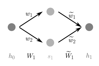
Figure 3.7: One-layer augmented neural network architecture $\Phi\in\Xi^{\infty}_{\textup{A}}(\mathbb{R},\mathbb{R})$ of Example 3.27.

In the following we show, that the set of weights

$$\mathcal{W}_{2}\coloneqq\{v\in\mathbb{R}^{7}\setminus(\mathcal{W}_{0}\cup\mathcal{W}_{1}):\;\exists\textup{ critical point }x^{\ast}\in\mathbb{R}\textup{ with }g(v,x^{\ast})=0\},$$

such that $\Phi$ has a degenerate critical point, has Lebesgue measure zero. To that purpose assume there exist weights $v\in\mathbb{R}^{7}\setminus(\mathcal{W}_{0}\cup\mathcal{W}_{1})$, such that $\Phi$ has a degenerate critical point $x^{\ast}$. We notice that by Theorem 3.22 a non-degenerate critical point perturbs to a non-degenerate critical point under small perturbation of the weights. Hence, if we aim to find degenerate critical points in a neighborhood of the considered weights $v\in\mathbb{R}^{7}\setminus(\mathcal{W}_{0}\cup\mathcal{W}_{1})$, the only possibility is that the degenerate critical point $x^{\ast}$ perturbs to a degenerate critical point. For $\varepsilon>0$ sufficiently small, consider the modified weights

$$\bar{v}(v,\varepsilon)=v+\left(\varepsilon,0,\delta(v,\varepsilon),0,0,0,0\right)^{\top}=\left(w_{1}+\varepsilon,w_{2},\widetilde{w}_{1}+\delta(v,\varepsilon),\widetilde{w}_{2},b_{11},b_{12},\tilde{b}_{1}\right)^{\top}\in\mathbb{R}^{7},$$

where

$$\delta(v,\varepsilon)=\widetilde{w}_{1}\left(\frac{w_{1}}{w_{1}+\varepsilon}\frac{1+\exp(-(w_{1}+\varepsilon)x^{\ast}-b_{11})}{1+\exp(-s_{1}^{\ast})}-1\right),$$ (3.10)

such that

$$\frac{w_{1}\widetilde{w}_{1}}{1+\exp(-s_{1}^{\ast})}=\frac{(w_{1}+\varepsilon)(\widetilde{w}_{1}+\delta(v,\varepsilon))}{1+\exp(-(w_{1}+\varepsilon)x^{\ast}-b_{11})}.$$

Hence, if and only if $x^{\ast}$ is a critical point of the network with weights $v$, then $x^{\ast}$ is also a critical point of the network with weights $\bar{v}$. It holds

$$\frac{\partial g(\bar{v}(v,\varepsilon),x^{\ast})}{\partial\varepsilon} =-\widetilde{w}_{2}x^{\ast}\exp(-(w_{1}+\varepsilon)x^{\ast}-b_{11})+\frac{\partial\delta(v,\varepsilon)}{\partial\varepsilon}\exp(-s_{2}^{\ast})$$

$$=-\widetilde{w}_{2}x^{\ast}\exp(-(w_{1}+\varepsilon)x^{\ast}-b_{11})+\left(-\frac{\widetilde{w}_{1}w_{1}}{(w_{1}+\varepsilon)^{2}}\frac{1+\exp(-(w_{1}+\varepsilon)x^{\ast}-b_{11})}{1+\exp(-s_{1}^{\ast})}\right.$$

$$\hskip 11.38109pt\left.-\frac{\widetilde{w}_{1}w_{1}x^{\ast}}{w_{1}+\varepsilon}\frac{\exp(-(w_{1}+\varepsilon)x^{\ast}-b_{11})}{1+\exp(-s_{1}^{\ast})}\right)\exp(-s_{2}^{\ast}),$$

which yields evaluated at $\varepsilon=0$:

$$\frac{\partial g(\bar{v}(v,0),x^{\ast})}{\partial\varepsilon} =-\widetilde{w}_{2}x^{\ast}\exp(-s_{1}^{\ast})-\frac{\widetilde{w}_{1}}{w_{1}}\exp(-s_{2}^{\ast})-\widetilde{w}_{1}x^{\ast}\frac{\exp(-s_{1}^{\ast})\exp(-s_{2}^{\ast})}{1+\exp(-s_{1}^{\ast})}$$

$$=-x^{\ast}(\widetilde{w}_{2}\exp(-s_{1}^{\ast})+\widetilde{w}_{1}\exp(-s_{2}^{\ast}))-\frac{\widetilde{w}_{1}}{w_{1}}\exp(-s_{2}^{\ast})+\widetilde{w}_{1}x^{\ast}\frac{\exp(-s_{2}^{\ast})}{1+\exp(-s_{1}^{\ast})}$$

$$=\frac{\widetilde{w}_{1}\exp(-s_{2}^{\ast})}{w_{1}(1+\exp(-s_{1}^{\ast}))}\left(1+\exp(-w_{1}h(v)-b_{11})+w_{1}h(v)\right)$$

where we used in the last line the property $g(v,x^{\ast})=0$, such that the first summand vanishes, and we replaced $x^{\ast}$ by $h(v)$ in the second summand. As $v\in\mathbb{R}^{7}\setminus(\mathcal{W}_{0}\cup\mathcal{W}_{1})$, it holds

$$\frac{\partial g(\bar{v}(v,0),x^{\ast})}{\partial\varepsilon}\neq 0.$$ (3.11)

For $\varepsilon>0$ sufficiently small we can deduce from $g(v,x^{\ast})=0$ and (3.11) that $g(\bar{v}(v,\varepsilon),x^{\ast})\neq 0$, such that $x^{\ast}$ is a non-degenerate critical point for the modified weights $\bar{v}$. From (3.10) it follows that for every $\mu>0$, the parameter $\varepsilon>0$ can be chosen small enough, such that $|\delta(v,\varepsilon)|<\mu$. Hence, we found a point $\bar{v}$ in a $\mu$-neighborhood of $v\in\mathcal{W}_{2}$, which is not contained in $\mathcal{W}_{2}$. Consequently $\mathcal{W}_{2}$ must have zero Lebesgue measure in $\mathbb{R}^{7}$ and $\Phi$ is a Morse function for all weighs in $\mathbb{R}^{7}\setminus(\mathcal{W}_{0}\cup\mathcal{W}_{1}\cup\mathcal{W}_{2})$, where $\mathcal{W}_{0}\cup\mathcal{W}_{1}\cup\mathcal{W}_{2}$ is a set of Lebesgue measure zero in $\mathbb{R}^{7}$.

3.5 Analysis of Bottleneck Architectures

In the last section, we proved Theorem 3.25 and showed regularity of the critical points of augmented neural networks. As mentioned in Remark 3.26, the theorem can also be applied to neural networks with a bottleneck, if they have a specific structure. In the following we study different types of neural networks with a bottleneck, and show that they can be of class $(\mathcal{C}1)^{k}(\mathcal{X},\mathbb{R})$ , $(\mathcal{C}2)^{k}(\mathcal{X},\mathbb{R})$ or $(\mathcal{C}3)^{k}(\mathcal{X},\mathbb{R})$. The main difference between the types of bottlenecks defined in the following theorem are if the neural network has an augmented part and if the assumptions specified in Remark 3.26 are fulfilled.

Theorem 3.28.

Let $\Phi\in\Xi_{\textup{B}}^{k}(\mathcal{X},\mathbb{R})$, $k\geq 2$, $\mathcal{X}\subset\mathbb{R}^{n}$ be a classical feed-forward neural network with weight matrices $W=(W_{1},\widetilde{W}_{1},\ldots,W_{L},\widetilde{W}_{L})=(V_{1},\ldots,V_{2L})\in\mathbb{W}$. Assume that $\Phi$ has its first bottleneck in layer $g_{j^{\ast}}\in\mathbb{R}^{d_{j^{\ast}}}$. Define for $l\in\{1,\ldots,2L-1\}$ the matrix product

$$Z_{l}(x)\coloneqq\widetilde{W}_{L}\Psi_{L}(s_{L})W_{L}\ldots V_{l+1}\in\mathbb{R}^{1\times d_{l}},$$

where $V_{l+1}=W_{l/2+1}$ if $l$ is even and $V_{l+1}=\widetilde{W}_{(l+1)/2}$ if $l$ is odd. $Z_{l}(x)$ is the product of all matrices occurring in the gradient defined in Lemma 3.17 until $V_{l+1}$.

1. Let the first bottleneck of $\Phi$ be non-augmented, i.e. $n=d_{0}\geq\ldots>d_{j^{\ast}}$ and let $Z_{j^{\ast}}(x)\neq 0$ for all $x\in\mathcal{X}$. If $W\in\mathbb{W}^{\ast}$, $\Phi$ is of class $(\mathcal{C}1)^{k}(\mathcal{X},\mathbb{R})$. Consequently for all set of weights $(\textup{vecm}(W);\textup{stk}(B))\in\mathbb{R}^{N_{W}+N_{B}}$, $W\in\mathbb{W}$, $b\in\mathbb{B}$, except possibly for a zero set in $\mathbb{R}^{N_{W}+N_{B}}$ w.r.t. the Lebesgue measure, $\Phi$ is of class $(\mathcal{C}1)^{k}(\mathcal{X},\mathbb{R})$.

2. Let the first bottleneck of $\Phi$ be non-augmented, i.e. $n=d_{0}\geq\ldots>d_{j^{\ast}}$ and denote the set of points $x\in\mathcal{X}$ such that $Z_{j^{\ast}}(x)=0$ by $\mathcal{X}^{\ast}\neq\varnothing$. Then every critical point $x^{\ast}\in\mathcal{X}^{\ast}$ is degenerate, such that $\Phi$ is of class $(\mathcal{C}3)^{k}(\mathcal{X},\mathbb{R})$.

3. Let the first bottleneck of $\Phi$ be augmented, i.e. there exists an index $i^{\ast}<j^{\ast}$ with $n=d_{0}\leq\ldots<d_{i^{\ast}}$ and let $Z_{i^{\ast}}(x)\neq 0$ for all $x\in\mathcal{X}$. Then $\Phi$ is for all weights $(\textup{vecm}(W);\textup{stk}(B))\in\mathbb{R}^{N_{W}+N_{B}}$, $W\in\mathbb{W}^{\ast}$, $b\in\mathbb{B}$, except possibly for a zero set in $\mathbb{R}^{N_{W}+N_{B}}$ w.r.t. the Lebesgue measure, of class $(\mathcal{C}1)^{k}(\mathcal{X},\mathbb{R})$ or $(\mathcal{C}2)^{k}(\mathcal{X},\mathbb{R})$. The same statement holds if $\mathbb{W}$ is replaced by $\mathbb{W}^{\ast}$.

4. Let the first bottleneck of $\Phi$ be augmented, i.e. there exists an index $i^{\ast}<j^{\ast}$ with $n=d_{0}\leq\ldots<d_{i^{\ast}}$ and and denote the set of points $x\in\mathcal{X}$ such that $Z_{i^{\ast}}(x)=0$ by $\mathcal{X}^{\ast}\neq\varnothing$. Then $x^{\ast}\in\mathcal{X}^{\ast}$ can be either degenerate or non-degenerate, so $\Phi$ is of class $(\mathcal{C}2)^{k}(\mathcal{X},\mathbb{R})$ or $(\mathcal{C}3)^{k}(\mathcal{X},\mathbb{R})$.

Proof.

Let $\Phi\in\Xi^{k}_{\textup{B}}(\mathcal{X},\mathbb{R})$, with weight matrices $W=(W_{1},\widetilde{W}_{1},\ldots,W_{L},\widetilde{W}_{L})=(V_{1},\ldots,V_{2L})\in\mathbb{W}$. By definition, there exist layers $g_{i}^{\ast}$, $g_{j}^{\ast}$ and $g_{l}^{\ast}$ with $0\leq i^{\ast}<j^{\ast}<l^{\ast}\leq 2L$, such that $d_{i}^{\ast}>d_{j}^{\ast}$ and $d_{j}^{\ast}<d_{l}^{\ast}$. The network gradient is by Lemma 3.17 given by

$$\nabla\Phi(x)^{\top} =\widetilde{W}_{L}\Psi_{L}(s_{L})W_{L}\ldots V_{l+1}V_{l}\ldots\widetilde{W}_{1}\Psi_{1}(s_{1})W_{1}$$

$$=V_{2L}\Psi_{L}(s_{L})V_{2L-1}\ldots V_{l+1}V_{l}\ldots V_{2}\Psi_{1}(s_{1})V_{1}$$

with $l\in\{1,\ldots,2L-1\}$, where $V_{l}=\widetilde{W}_{l/2}\in\mathbb{R}^{d_{l}\times d_{l-1}}$, $V_{l+1}=W_{l/2+1}\in\mathbb{R}^{d_{l+1}\times d_{l}}$ if $l$ is even and $V_{l}=\Psi_{(l+1)/2}(s_{(l+1)/2})\in\mathbb{R}^{d_{l}\times d_{l}}$, $V_{l+1}=\widetilde{W}_{(l+1)/2}\in\mathbb{R}^{d_{l+1}\times d_{l}}$ if $l$ is odd. We denote by $Z_{l}(x)\in\mathbb{R}^{1\times d_{l}}$ the matrix product $\widetilde{W}_{L}\ldots V_{l+1}$ and by $Y_{l}(x)\in\mathbb{R}^{d_{l}\times n}$ the matrix product $V_{l}\ldots W_{1}$, such that

$$\nabla\Phi(x)^{\top}=Z_{l}(x)Y_{l}(x)\in\mathbb{R}^{1\times n}.$$ (3.12)

For case (a), we assume that $n=d_{0}\geq\ldots>d_{j^{\ast}}$ and that $Z_{j^{\ast}}(x)\neq 0$ for all $x\in\mathcal{X}$. If $W\in\mathbb{W}^{\ast}$, the assumption $n=d_{0}\geq\ldots>d_{j^{\ast}}$ implies that the dimensions of the matrices in the product $Y_{j^{\ast}}(x)$ are monotonically increasing, such that by Lemma 3.10 $Y_{j^{\ast}}(x)$ has for every $x\in\mathcal{X}$ full rank $d_{j^{\ast}}$. As $Z_{j^{\ast}}(x)\neq 0$ for all $x\in\mathcal{X}$ also the matrix $Z_{j^{\ast}}(x)$ has always full rank 1, such that another application of Lemma 3.10 implies that $\nabla\Phi(x)$ has for every $x\in\mathcal{X}$ full rank. Consequently no critical point exists and $\Phi$ is of class $(\mathcal{C}1)^{k}(\mathcal{X},\mathbb{R})$ if $W\in\mathbb{W}^{\ast}$. The same argumentation as in Theorem 3.18 for non-augmented neural networks shows that for all set of weights $(\textup{vecm}(W);\textup{stk}(B))\in\mathbb{R}^{N_{W}+N_{B}}$, except possibly for a zero set in $\mathbb{R}^{N_{W}+N_{B}}$ w.r.t. the Lebesgue measure, $\Phi$ is of class $(\mathcal{C}1)^{k}(\mathcal{X},\mathbb{R})$.

For case (b), we assume that $n=d_{0}\geq\ldots>d_{j^{\ast}}$ and that $Z_{j^{\ast}}(x^{\ast})=0$ for all $x^{\ast}\in\mathcal{X}^{\ast}\neq\varnothing$. The structure of the gradient (3.12) implies that every $x^{\ast}\in\mathcal{X}^{\ast}$ is a critical point of $\Phi$. The $i$-th row $[H_{\Phi}(x)^{\top}]_{i}^{\top}$ of the Hessian $H_{\Phi}(x)\in\mathbb{R}^{n\times n}$ evaluated at a critical point $x^{\ast}\in\mathcal{X}^{\ast}$ is given by

$$[H_{\Phi}(x^{\ast})^{\top}]_{i}^{\top}=\frac{\partial}{\partial x_{i}}\left[Z_{j^{\ast}}(x)Y_{j^{\ast}}(x)\right]\bigg{|}_{x=x^{\ast}}=\frac{\partial Z_{j^{\ast}}}{\partial x_{i}}(x^{\ast})Y_{j^{\ast}}(x^{\ast})+Z_{j^{\ast}}(x^{\ast})\frac{\partial Y_{j^{\ast}}}{\partial x_{i}}(x^{\ast})=\frac{\partial Z_{j^{\ast}}}{\partial x_{i}}(x^{\ast})Y_{j^{\ast}}(x^{\ast}),$$

as $Z_{j^{\ast}}(x^{\ast})=0$ for $x^{\ast}\in\mathcal{X}^{\ast}$. The $n$ vectors $\frac{\partial Z_{j^{\ast}}}{\partial x_{i}}(x^{\ast})\in\mathbb{R}^{1\times d_{j^{\ast}}}$, $i\in\{1,\ldots,n\}$ are linearly dependent as $d_{j^{\ast}}<n$. Hence, there exist $\alpha_{1},\ldots,\alpha_{n}$ not all equal to zero such that

$$\sum_{i=1}^{n}\alpha_{i}\frac{\partial Z_{j^{\ast}}}{\partial x_{i}}(x^{\ast})=0\in\mathbb{R}^{1\times d_{j^{\ast}}}.$$

As matrix multiplication is distributive, it follows

$$\sum_{i=1}^{n}\alpha_{i}[H_{\Phi}(x^{\ast})^{\top}]_{i}^{\top}=\sum_{i=1}^{n}\alpha_{i}\left[\frac{\partial Z_{j^{\ast}}}{\partial x_{i}}(x^{\ast})Y_{j^{\ast}}(x^{\ast})\right]=\left[\sum_{i=1}^{n}\alpha_{i}\frac{\partial Z_{j^{\ast}}}{\partial x_{i}}(x^{\ast})\right]Y_{j^{\ast}}(x^{\ast})=0\in\mathbb{R}^{n},$$

which implies that the rows of the Hessian $H_{\Phi}(x^{\ast})$ are linearly dependent. Consequently $H_{\Phi}(x^{\ast})$ has not full rank and at least one eigenvalue is zero, such that the critical point $x^{\ast}$ is degenerate. As $x^{\ast}$ was arbitrary, it follows that every critical point of $\Phi$ is degenerate and $\Phi$ is of class $(\mathcal{C}3)^{k}(\mathcal{X},\mathbb{R})$.

For case (c) we assume that there exists an index $i^{\ast}<j^{\ast}$ with $n=d_{0}\leq\ldots<d_{i^{\ast}}$ and that $Z_{i^{\ast}}(x)\neq 0$ for all $x\in\mathcal{X}$. We aim to show the statement of Theorem 3.25 for the considered bottleneck architecture, as proposed in Remark 3.26. To that purpose, we compare the matrices $\overline{Y}$ and $\overline{Z}$ of the proof of Theorem 3.25 with the matrices $Y_{i^{\ast}}(x)$ and $Z_{i^{\ast}}(x)$ defined in this proof by identifying the index $l^{\ast}$ of Theorem 3.25 with the index $i^{\ast}$ considered here. If $i^{\ast}$ is even, equation (3.4) implies that $Y_{i^{\ast}}(x)=\overline{Y}^{\top}$ and $Z_{i^{\ast}}(x)=\overline{Z}^{\top}W_{i^{\ast}/2+1}$, and if $i^{\ast}$ is odd, (3.6) shows that $Y_{i^{\ast}}(x)=\overline{Y}^{\top}$ and $Z_{i^{\ast}}(x)=\overline{Z}^{\top}\widetilde{W}_{(i^{\ast}+1)2}$. If $W\in\mathbb{W}^{\ast}$, the assumption $n=d_{0}\leq\ldots<d_{j^{\ast}}$ implies that the dimensions of the matrices in the product $Y_{i^{\ast}}(x)$ are monotonically decreasing, such that by Lemma 3.10 $Y_{i^{\ast}}(x)$ has for every $x\in\mathcal{X}$ full rank $n$, and hence also $\overline{Y}$ has full rank $n$. The assumption $Z_{i^{\ast}}(x)\neq 0$ for all $x\in\mathcal{X}$ implies that it is necessary that $\overline{Z}\neq 0$ for all $x\in\mathcal{X}$, so $\overline{Z}$ has full rank 1. By Remark 3.26, the proof of Theorem 3.25 works analogously for the considered neural network $\Phi$ with a bottleneck, such that $\Phi$ is for all weights $(\textup{vecm}(W);\textup{stk}(B))\in\mathbb{R}^{N_{W}+N_{B}}$, $W\in\mathbb{W}^{\ast}$, $b\in\mathbb{B}$, except possibly for a zero set in $\mathbb{R}^{N_{W}+N_{B}}$ w.r.t. the Lebesgue measure, of class $(\mathcal{C}1)^{k}(\mathcal{X},\mathbb{R})$ or $(\mathcal{C}2)^{k}(\mathcal{X},\mathbb{R})$. As $\textup{vecm}(\mathbb{W}\setminus\mathbb{W}^{\ast})\times\textup{stk}(\mathbb{B})$ is a zero set w.r.t the Lebesgue measure in $\mathbb{R}^{N_{W}+N_{B}}$ and the union of two sets with measure zero has again measure zero, the same statement holds if $\mathbb{W}^{\ast}$ is replaced by $\mathbb{W}$.

For case (d) we assume that there exists an index $i^{\ast}<j^{\ast}$ with $n=d_{0}\leq\ldots<d_{i^{\ast}}$ and that $Z_{i^{\ast}}(x^{\ast})=0$ for all $x^{\ast}\in\mathcal{X}^{\ast}\neq\varnothing$. The structure of the gradient (3.12) implies that every $x^{\ast}\in\mathcal{X}^{\ast}$ is a critical point of $\Phi$. As in case (b), the $i$-th row $[H_{\Phi}(x)^{\top}]_{i}^{\top}$ of the Hessian $H_{\Phi}(x)\in\mathbb{R}^{n\times n}$ evaluated at a critical point $x^{\ast}\in\mathcal{X}^{\ast}$ is given by

$$[H_{\Phi}(x^{\ast})^{\top}]_{i}^{\top}=\frac{\partial}{\partial x_{i}}\left[Z_{j^{\ast}}(x)Y_{j^{\ast}}(x)\right]\bigg{|}_{x=x^{\ast}}=\frac{\partial Z_{j^{\ast}}}{\partial x_{i}}(x^{\ast})Y_{j^{\ast}}(x^{\ast})+Z_{j^{\ast}}(x^{\ast})\frac{\partial Y_{j^{\ast}}}{\partial x_{i}}(x^{\ast})=\frac{\partial Z_{j^{\ast}}}{\partial x_{i}}(x^{\ast})Y_{j^{\ast}}(x^{\ast}),$$

as $Z_{j^{\ast}}(x^{\ast})=0$ for $x^{\ast}\in\mathcal{X}^{\ast}$. As $d_{j^{\ast}}>n$, the $n$ vectors $\frac{\partial Z_{j^{\ast}}}{\partial x_{i}}(x^{\ast})\in\mathbb{R}^{1\times d_{j^{\ast}}}$, $i\in\{1,\ldots,n\}$ can be linearly dependent, but they can also be linearly independent. This implies in analogy to case (b), that the Hessian matrix can have full rank, but does not need to. In Example 3.29 we show that both cases are possible. As $\Phi$ always has at least one critical point, it follows that $\Phi$ is of class $(\mathcal{C}2)^{k}(\mathcal{X},\mathbb{R})$ or $(\mathcal{C}3)^{k}(\mathcal{X},\mathbb{R})$. ∎

We end this section with a few examples of neural networks with bottleneck architectures, which show that all cases mentioned in Theorem 3.28 exist. The considered architectures are visualized in Figure 3.8.

Example 3.29.

We present for each of the cases (a)-(d) of Theorem 3.28 a two-layer neural network architecture $\Phi\in\Xi_{\textup{B}}^{k}(\mathcal{X},\mathbb{R})$, $k\geq 2$ with full rank weight matrices $W\in\mathbb{W}^{\ast}$ and nonlinear, strictly monotonically increasing activation functions.

1. Let $\mathcal{X}=\mathbb{R}^{2}$, $L=2$ and $\Phi$ be defined by the weight matrices

   $$W_{1}=(1,1),\quad\widetilde{W}_{1}=\begin{pmatrix}1\\ 1\end{pmatrix},\quad W_{2}=(1,1),\quad\widetilde{W}_{2}=1$$

   and arbitrary biases $b\in\mathbb{B}$, see Figure 3.88(a). Then $\Phi$ has a non-augmented bottleneck at layer $g_{1}=s_{1}$, so $j^{\ast}=1$. It holds

   $$Z_{1}(x)=1\cdot\Psi_{2}(s_{2})\cdot(1,1)\cdot\begin{pmatrix}1\\ 1\end{pmatrix}=2\sigma_{2}^{\prime}(s_{2})\neq 0\qquad\forall\,x\in\mathcal{X}.$$

   By Theorem 3.28(a), $\Phi$ is off class $(\mathcal{C}1)^{k}(\mathcal{X},\mathbb{R})$. As

   $$\nabla\Phi(x)^{\top}=1\cdot\Psi_{2}(s_{2})\cdot(1,1)\cdot\begin{pmatrix}1\\ 1\end{pmatrix}\cdot\Psi_{1}(s_{1})\cdot(1,1)=(2\sigma_{2}^{\prime}(s_{2})\sigma_{1}^{\prime}(s_{1}),2\sigma_{2}^{\prime}(s_{2})\sigma_{1}^{\prime}(s_{1}))\neq(0,0)$$

   for all $x\in\mathcal{X}$, we verified that $\Phi$ cannot have any critical points.

2. Let $\mathcal{X}=\mathbb{R}^{2}$, $L=2$ and $\Phi$ be defined by the weight matrices

   $$W_{1}=(1,1),\quad\widetilde{W}_{1}=\begin{pmatrix}1\\ 0\end{pmatrix},\quad W_{2}=(0,1),\quad\widetilde{W}_{2}=1$$

   and arbitrary biases $b\in\mathbb{B}$, see Figure 3.88(b). Then $\Phi$ has a non-augmented bottleneck at layer $g_{1}=s_{1}$, so $j^{\ast}=1$. It holds

   $$Z_{1}(x)=1\cdot\Psi_{2}(s_{2})\cdot(0,1)\cdot\begin{pmatrix}1\\ 0\end{pmatrix}=0\qquad\forall\,x\in\mathcal{X}.$$

   By Theorem 3.28(b), $\Phi$ is off class $(\mathcal{C}3)^{k}(\mathcal{X},\mathbb{R})$. As

   $$\nabla\Phi(x)^{\top}=1\cdot\Psi_{2}(s_{2})\cdot(0,1)\cdot\begin{pmatrix}1\\ 0\end{pmatrix}\cdot\Psi_{1}(s_{1})\cdot(1,1)=(2\sigma_{2}^{\prime}(s_{2})\sigma_{1}^{\prime}(s_{1}),2\sigma_{2}^{\prime}(s_{2})\sigma_{1}^{\prime}(s_{1}))=(0,0)$$

   for all $x\in\mathcal{X}$, the gradient $\nabla\Phi$ is the constant zero function, hence the Hessian matrix $H_{\Phi}$ is also zero everywhere. Hence, we verified that $\Phi$ is of class $(\mathcal{C}3)^{k}(\mathcal{X},\mathbb{R})$, as every critical point is degenerate.

   .

   

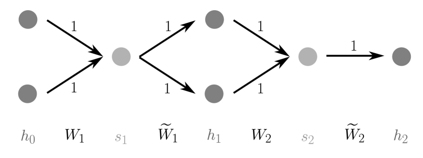
   (a) Example of a neural network $\Phi\in\Xi_{\textup{B}}^{k}(\mathbb{R}^{2},\mathbb{R})$ with a non-augmented bottleneck at layer $s_{1}$, which is of class $(\mathcal{C}1)^{k}(\mathcal{X},\mathbb{R})$.

   .

   

   (b) Example of a neural network $\Phi\in\Xi_{\textup{B}}^{k}(\mathbb{R}^{2},\mathbb{R})$ with a non-augmented bottleneck at layer $s_{1}$, which is of class $(\mathcal{C}3)^{k}(\mathcal{X},\mathbb{R})$.

   .

   .

   

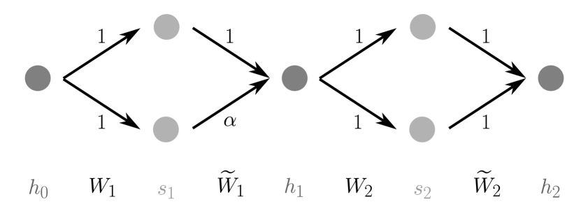
   (c) Example of a neural network $\Phi\in\Xi_{\textup{B}}^{k}(\mathbb{R},\mathbb{R})$ with an augmented bottleneck at layer $h_{1}$, which is depending on $\alpha$ of class $(\mathcal{C}1)^{k}(\mathcal{X},\mathbb{R})$ or $(\mathcal{C}2)^{k}(\mathcal{X},\mathbb{R})$.

   .

   

   (d) Example of a neural network $\Phi\in\Xi_{\textup{B}}^{k}(\mathbb{R},\mathbb{R})$ with an augmented bottleneck at layer $h_{1}$, which is depending on $\alpha$ and $\beta$ of class $(\mathcal{C}1)^{k}(\mathcal{X},\mathbb{R})$, $(\mathcal{C}2)^{k}(\mathcal{X},\mathbb{R})$ or $(\mathcal{C}3)^{k}(\mathcal{X},\mathbb{R})$

   .

   Figure 3.8: Two-layer neural network architectures $\Phi\in\Xi_{\textup{B}}^{k}(\mathcal{X},\mathbb{R})$ with full rank weight matrices $W\in\mathbb{W}^{\ast}$ and nonlinear, strictly monotonically increasing activation functions, which are analyzed in Example 3.29.

3. Let $\mathcal{X}=\mathbb{R}$, $L=2$ and $\Phi$ be defined by the weight matrices

   $$W_{1}=\begin{pmatrix}1\\ 1\end{pmatrix},\quad\widetilde{W}_{1}=(1,\alpha),\quad W_{2}=\begin{pmatrix}1\\ 1\end{pmatrix},\quad\widetilde{W}_{2}=(1,1)$$

   with $\alpha\in\mathbb{R}$ specified in the following and arbitrary biases $b\in\mathbb{B}$, see Figure 3.88(c). Then $\Phi$ has an augmented bottleneck at layer $g_{2}=h_{1}$, so $i^{\ast}=1$ and $j^{\ast}=2$. It holds

   $$Z_{1}(x) =(1,1)\cdot\Psi_{2}(s_{2})\cdot\begin{pmatrix}1\\ 1\end{pmatrix}\cdot(1,\alpha)$$

   $$=\big{(}[\sigma_{2}]_{1}^{\prime}([s_{2}]_{1})+[\sigma_{2}]_{2}^{\prime}([s_{2}]_{2}),\alpha([\sigma_{2}]_{1}^{\prime}([s_{2}]_{1})+[\sigma_{2}]_{2}^{\prime}([s_{2}]_{2}))\big{)}\neq 0\qquad\forall\,x\in\mathcal{X},$$

   as the sum of two strictly monotonically increasing functions is again strictly monotonically increasing. By Theorem 3.28(c), $\Phi$ is for all set of weights, except possibly for a zero set w.r.t. the Lebesgue measure, of class $(\mathcal{C}1)^{k}(\mathcal{X},\mathbb{R})$ or $(\mathcal{C}2)^{k}(\mathcal{X},\mathbb{R})$. We show that both cases are possible. It holds

   $$\nabla\Phi(x)^{\top} =(1,1)\cdot\Psi_{2}(s_{2})\cdot\begin{pmatrix}1\\ 1\end{pmatrix}\cdot(1,\alpha)\cdot\Psi_{1}(s_{1})\cdot\begin{pmatrix}1\\ 1\end{pmatrix}$$

   $$=\big{(}[\sigma_{2}]_{1}^{\prime}([s_{2}]_{1})+[\sigma_{2}]_{2}^{\prime}([s_{2}]_{2})\big{)}\cdot\big{(}[\sigma_{1}]_{1}^{\prime}([s_{1}]_{1})+\alpha[\sigma_{1}]_{2}^{\prime}([s_{1}]_{2})\big{)}.$$

   We define the set

   $$\mathcal{A}=\left\{a\in\mathbb{R}:a=-\frac{[\sigma_{1}]_{1}^{\prime}([s_{1}]_{1})}{[\sigma_{1}]_{2}^{\prime}([s_{1}]_{2})}\textup{ for some }x\in\mathbb{R}\right\}\subset\mathbb{R}_{<0},$$

   which is non-empty and by construction of the network independent of the choice of $\alpha$. Also $\mathbb{R}\setminus\mathcal{A}$ is non-empty as $\mathcal{A}\subset\mathbb{R}_{<0}$. If $\alpha\in\mathbb{R}\setminus\mathcal{A}$, then $\nabla\Phi(x)\neq 0$ for all $x\in\mathcal{X}$, such that $\Phi$ is of class $(\mathcal{C}1)^{k}(\mathcal{X},\mathbb{R})$. If the activation functions $[\sigma_{1}]_{1}$ and $[\sigma_{1}]_{2}$ are non-linear, then $[\sigma_{1}]_{1}^{\prime}$ and $[\sigma_{1}]_{2}^{\prime}$ are non-constant, such that $\mathcal{A}$ has non-zero Lebesgue measure. Hence, for all $\alpha\in\mathcal{A}$, except possibly for a zero set w.r.t. the Lebesgue measure, Theorem 3.28(c) implies that $\Phi$ is of class $(\mathcal{C}2)^{k}(\mathcal{X},\mathbb{R})$ and has only non-degenerate critical points.

4. Let $\mathcal{X}=\mathbb{R}$, $L=2$ and $\Phi$ be defined by the weight matrices

   $$W_{1}=\begin{pmatrix}1\\ 1\end{pmatrix},\quad\widetilde{W}_{1}=(1,\alpha),\quad W_{2}=\begin{pmatrix}1\\ 1\end{pmatrix},\quad\widetilde{W}_{2}=(1,\beta)$$

   with $\alpha,\beta\in\mathbb{R}$ specified in the following and arbitrary biases $b\in\mathbb{B}$, see Figure 3.88(d). It holds

   $$Z_{1}(x) =(1,\beta)\cdot\Psi_{2}(s_{2})\cdot\begin{pmatrix}1\\ 1\end{pmatrix}\cdot(1,\alpha)$$

   $$=\big{(}[\sigma_{2}]_{1}^{\prime}([s_{2}]_{1})+\beta[\sigma_{2}]_{2}^{\prime}([s_{2}]_{2}),\alpha([\sigma_{2}]_{1}^{\prime}([s_{2}]_{1})+\beta[\sigma_{2}]_{2}^{\prime}([s_{2}]_{2}))\big{)}.$$

   We define the set

   $$\mathcal{B}_{\alpha}=\left\{b\in\mathbb{R}:b=-\frac{[\sigma_{2}]_{1}^{\prime}([s_{2}]_{1})}{[\sigma_{2}]_{2}^{\prime}([s_{2}]_{2})}\textup{ for some }x\in\mathbb{R}\right\},$$

   which is non-empty and by construction of the network dependent on the choice of $\alpha$, but independent of the choice of $\beta$. If $\beta\notin\mathcal{B}_{\alpha}$, the analysis of the neural network is the same as in case (c) and $\Phi$ can be of class $(\mathcal{C}1)^{k}(\mathcal{X},\mathbb{R})$ or $(\mathcal{C}2)^{k}(\mathcal{X},\mathbb{R})$. In the following we choose $\beta\in\mathcal{B}_{\alpha}$, such that for every choice of $\alpha,\beta$ there exist $x^{\ast}\in\mathbb{R}$ such that $Z_{1}(x^{\ast})=0$ and the assumptions of Theorem 3.28(d) are fulfilled. Consequently $\Phi$ is off class $(\mathcal{C}2)^{k}(\mathcal{X},\mathbb{R})$ or $(\mathcal{C}3)^{k}(\mathcal{X},\mathbb{R})$. We show that both cases are possible. It holds

   $$\nabla\Phi(x)^{\top} =(1,\beta)\cdot\Psi_{2}(s_{2})\cdot\begin{pmatrix}1\\ 1\end{pmatrix}\cdot(1,\alpha)\cdot\Psi_{1}(s_{1})\cdot\begin{pmatrix}1\\ 1\end{pmatrix}$$

   $$=\big{(}[\sigma_{2}]_{1}^{\prime}([s_{2}]_{1})+\beta[\sigma_{2}]_{2}^{\prime}([s_{2}]_{2})\big{)}\cdot\big{(}[\sigma_{1}]_{1}^{\prime}([s_{1}]_{1})+\alpha[\sigma_{1}]_{2}^{\prime}([s_{1}]_{2})\big{)}.$$

   As $\beta\in\mathcal{B}_{\alpha}$, for every choice of $\alpha,\beta$ there exist at least one critical point $x^{\ast}\in\mathbb{R}$. The Hessian matrix $H_{\Phi}(x)$ is by the product rule given by

   $$H_{\Phi}(x) =\left([\sigma_{2}]_{1}^{\prime\prime}([s_{2}]_{1})\frac{\partial[s_{2}]_{1}}{\partial x}+\beta[\sigma_{2}]_{2}^{\prime\prime}([s_{2}]_{2})\frac{\partial[s_{2}]_{2}}{\partial x}\right)\cdot\left([\sigma_{1}]_{1}^{\prime}([s_{1}]_{1})+\alpha[\sigma_{1}]_{2}^{\prime}([s_{1}]_{2})\right)$$

   $$\;\;\;+\left([\sigma_{2}]_{1}^{\prime}([s_{2}]_{1})+\beta[\sigma_{2}]_{2}^{\prime}([s_{2}]_{2})\right)\cdot\left([\sigma_{1}]_{1}^{\prime\prime}([s_{1}]_{1})\frac{\partial[s_{1}]_{1}}{\partial x}+\alpha[\sigma_{1}]_{2}^{\prime\prime}([s_{1}]_{2})\frac{\partial[s_{1}]_{2}}{\partial x}\right).$$

   Evaluated at a critical point $x^{\ast}$ it holds

   $$H_{\Phi}(x^{\ast})=\left([\sigma_{2}]_{1}^{\prime\prime}([s_{2}]_{1})\frac{\partial[s_{2}]_{1}}{\partial x}+\beta[\sigma_{2}]_{2}^{\prime\prime}([s_{2}]_{2})\frac{\partial[s_{2}]_{2}}{\partial x}\right)\cdot\left([\sigma_{1}]_{1}^{\prime}([s_{1}]_{1})+\alpha[\sigma_{1}]_{2}^{\prime}([s_{1}]_{2})\right)$$

   as $Z_{1}(x^{\ast})=0$. By choosing $\alpha\in\mathcal{A}$, which is defined in part (c), we can guarantee that the critical point $x^{\ast}$ can be degenerate, so it is possible that $\Phi$ is of class $(\mathcal{C}3)^{k}(\mathcal{X},\mathbb{R})$. To show that $\Phi$ can also be of class $(\mathcal{C}2)^{k}(\mathcal{X},\mathbb{R})$, we choose some $\alpha\in\mathbb{R}\setminus\mathcal{A}$, such that $[\sigma_{1}]_{1}^{\prime}([s_{1}]_{1})+\alpha[\sigma_{1}]_{2}^{\prime}([s_{1}]_{2})\neq 0$ for all $x\in\mathbb{R}$. $\alpha\in\mathbb{R}\setminus\mathcal{A}$ exists by part (c). If we choose for example soft-plus activation functions $[\sigma_{2}]_{1}(x)=[\sigma_{2}]_{2}(x)=\ln(1+\exp(x))$, then

   $$\frac{\partial[s_{2}]_{1}}{\partial x}=\frac{\partial[s_{2}]_{2}}{\partial x}=[\sigma_{1}]_{1}^{\prime}([s_{1}]_{1})+\alpha[\sigma_{1}]_{2}^{\prime}([s_{1}]_{2}),$$

   such that

   $$H_{\Phi}(x^{\ast}) =\left(\frac{\exp(-[s_{2}]_{1})}{(1+\exp(-[s_{2}]_{1}))^{2}}+\beta\frac{\exp(-[s_{2}]_{2})}{(1+\exp(-[s_{2}]_{2}))^{2}}\right)\cdot\left([\sigma_{1}]_{1}^{\prime}([s_{1}]_{1})+\alpha[\sigma_{1}]_{2}^{\prime}([s_{1}]_{2})\right)^{2}$$

   $$=\left(\frac{\exp(-[s_{2}]_{1})}{(1+\exp(-[s_{2}]_{1}))^{2}}-\frac{1+\exp(-[s_{2}]_{2})}{1+\exp(-[s_{2}]_{1})}\frac{\exp(-[s_{2}]_{2})}{(1+\exp(-[s_{2}]_{2}))^{2}}\right)$$

   $$\hskip 11.38109pt\cdot\left([\sigma_{1}]_{1}^{\prime}([s_{1}]_{1})+\alpha[\sigma_{1}]_{2}^{\prime}([s_{1}]_{2})\right)^{2}$$

   $$=\frac{1}{1+\exp(-[s_{2}]_{1})}\left(\frac{1}{1+\exp([s_{2}]_{1})}-\frac{1}{1+\exp([s_{2}]_{2})}\right)\cdot\left([\sigma_{1}]_{1}^{\prime}([s_{1}]_{1})+\alpha[\sigma_{1}]_{2}^{\prime}([s_{1}]_{2})\right)^{2}$$

   which is non-zero as long as $[s_{2}]_{1}\neq[s_{2}]_{2}$ as $\frac{1}{1+\exp(x)}$ is a monotonically decreasing function. As $s_{2}=W_{1}h_{1}+b_{2}$, variation of the bias $b_{2}\in\mathbb{R}^{2}$ guarantees that for all $b_{2}\in\mathbb{R}^{2}$, except possibly for a set of measure w.r.t. the Lebesgue measure in $\mathbb{R}^{2}$, it holds $[s_{2}]_{1}\neq[s_{2}]_{2}$. Hence, we showed the existence of a neural network architecture $\Phi$ which fulfills the assumptions of Theorem 3.28(d) and which is of class $(\mathcal{C}2)^{k}(\mathcal{X},\mathbb{R})$.

4 Neural ODEs

Each neural ODE architecture is based on the solution $h:\mathcal{I}\rightarrow\mathbb{R}^{m}$ of an initial value problem

$$\frac{\mathrm{d}h}{\mathrm{d}t}=f(h(t),t),\qquad h(0)=s\in\mathcal{S}\subset\mathbb{R}^{m},$$ (IVP)

with $f:\mathbb{R}^{m}\times\mathcal{I}\rightarrow\mathbb{R}^{m}$, where $\mathcal{I}\subset\mathbb{R}$ open denotes the maximal time interval of existence. We denote a solution with initial condition $h(0)=s$ by $h_{s}(t)$ to take into account the dependence on the initial data. Hereby $\varnothing\neq\mathcal{S}\subset\mathbb{R}^{m}$ is a non-zero set of initial conditions. The considered neural ODE architectures depend on the time-$T$ map $h_{s}(T)$ of (IVP), hence we always assume that the maximal time interval of existence fulfills $\mathcal{I}\supset[0,T]$. The vector field $f:\mathbb{R}^{m}\times\mathcal{I}\rightarrow\mathbb{R}^{m}$ is a continuous function, which can depend on parameters. As the results established in this work do not depend on the choice of the vector field, we consider no specific paramterization of $f$. First, we state a basic result from ODE theory regarding the regularity of the solution map of the initial value problem (IVP).

Lemma 4.1 ([8]).

Let $f\in C^{k,0}(\mathbb{R}^{m}\times\mathcal{I},\mathbb{R}^{m})$, $k\geq 0$ and assume $[0,T]\subset\mathcal{I}$. Then it holds for the time-$T$ map of the solution $h_{s}:\mathcal{I}\rightarrow\mathbb{R}^{m}$ of the initial value problem (IVP) that $h_{s}(T)\in C^{k}(\mathcal{S},\mathbb{R}^{m})$ and if $k\geq 1$, the solution curves are unique.

We need to assume the regularity of the vector field, to be able to differentiate the network and characterize if the neural ODE is a Morse function. The analysis is restricted to neural ODE architectures with scalar output, for more general networks, the results apply to the scalar components of the output. The architectures we consider have a linear layer before and after the time-$T$ map of the initial value problem resulting in the neural ODE architecture

$$\Phi:\mathcal{X}\mapsto\mathbb{R},\qquad\Phi(x)\coloneqq\widetilde{L}(h_{L(x)}(T))=\widetilde{W}\cdot h_{Wx+b}(T)+\tilde{b}=\widetilde{W}\cdot h_{s}(T)+\tilde{b},$$ (4.1)

where the first linear layer $L:\mathbb{R}^{n}\rightarrow\mathbb{R}^{m}$ is represented by a matrix $W\in\mathbb{R}^{m\times n}$ and a vector $b\in\mathbb{R}^{m}$ and the second linear layer $\widetilde{L}:\mathbb{R}^{m}\rightarrow\mathbb{R}$ is represented by a row vector $\widetilde{W}\in\mathbb{R}^{1\times m}$ and a scalar $\tilde{b}\in\mathbb{R}$. The intermediate layer, which defines the initial condition of (IVP) is calculated by $s=L(x)=Wx+b$. We define the set of initial conditions of (IVP) to be $\mathcal{S}\coloneqq L(\mathcal{X})$. Compared to classical feed-forward neural networks, the neural ODE architecture (4.1) has one inner linear layer corresponding to the weights $W_{1}$ and $b_{1}$, then an initial value problem evolves in the dimension $m$ of the intermediate layer $s\coloneqq Wx+b$ and then a second outer linear layer corresponding to the weights $\widetilde{W}_{L}$ and $\tilde{b}_{L}$ is applied to the time-$T$ map of (IVP). The regularity of the neural ODE architecture (4.1) follows directly from the regularity of the underlying initial value problem.

Lemma 4.2.

Let $f\in C^{k,0}(\mathbb{R}^{m}\times\mathcal{I},\mathbb{R}^{m})$, $k\geq 0$ and assume $[0,T]\subset\mathcal{I}$. Then it holds for the neural ODE architecture defined in (4.1) that $\Phi\in C^{k}(\mathcal{X},\mathbb{R})$.

Proof.

The result follows directly from Lemma 4.1. ∎

Definition 4.3.

For $k\geq 0$, the set of all scalar neural ODE architectures $\Phi:\mathcal{X}\rightarrow\mathbb{R}$, $\mathcal{X}\subset\mathbb{R}^{n}$ open, defined by (4.1) with vector field $f\in C^{k,0}(\mathbb{R}^{m}\times\mathcal{I},\mathbb{R}^{m})$ and $[0,T]\subset\mathcal{I}$, $\mathcal{I}\subset\mathbb{R}$ open, is denoted by $\textup{NODE}^{k}(\mathcal{X},\mathbb{R})\subset C^{k}(\mathcal{X},\mathbb{R})$.

4.1 Special Architectures

In the following, we subdivide the set of all neural ODE architectures $\text{NODE}^{k}(\mathcal{X},\mathbb{R})$ introduced in Definition 4.3 in three different classes: non-augmented neural ODEs, augmented neural ODEs and neural ODEs with a bottleneck.

Non-Augmented

We call a neural ODE $\Phi\in\text{NODE}^{k}(\mathcal{X},\mathbb{R})$ non-augmented, if $n\geq m$, i.e. the dimension of the ODE is smaller than the dimension of the input data. We require that the weight matrices of both linear layers have full rank, i.e. $\text{rank}(W)=m$ and $\text{rank}(\widetilde{W})=1$. The subset of non-augmented neural ODEs is denoted by

$$\textup{NODE}^{k}_{\textup{N}}(\mathcal{X},\mathbb{R})\coloneqq\left\{\Phi\in\textup{NODE}^{k}(\mathcal{X},\mathbb{R}):\Phi\textup{ is non-augmented}\right\}.$$

Augmented

We call a neural ODE $\Phi\in\text{NODE}^{k}(\mathcal{X},\mathbb{R})$ augmented, if $n<m$, i.e. the dimension of the ODE is larger than the dimension of the input data. We require that the weight matrices of both linear layers have full rank, i.e. $\text{rank}(W)=n$ and $\text{rank}(\widetilde{W})=1$. The subset of augmented neural ODEs is denoted by

$$\textup{NODE}^{k}_{\textup{A}}(\mathcal{X},\mathbb{R})\coloneqq\left\{\Phi\in\textup{NODE}^{k}(\mathcal{X},\mathbb{R}):\Phi\textup{ is augmented}\right\}.$$

Bottleneck

We say that a neural ODE $\Phi\in\text{NODE}^{k}(\mathcal{X},\mathbb{R})$ has a bottleneck, if at least one of the weight matrices of the two linear layeres has not full rank, i.e. $\text{rank}(W)<\min\{m,n\}$ or $\text{rank}(\widetilde{W})=0$. The subset of neural ODEs with a bottleneck is denoted by

$$\textup{NODE}^{k}_{\textup{B}}(\mathcal{X},\mathbb{R})\coloneqq\left\{\Phi\in\textup{NODE}^{k}(\mathcal{X},\mathbb{R}):\Phi\textup{ has a bottleneck}\right\}.$$

The three different types of neural ODEs are visualized in Figure 4.1. In the following we show that these three types of architectures build a disjoint subdivision of all classical feed-forward neural networks.

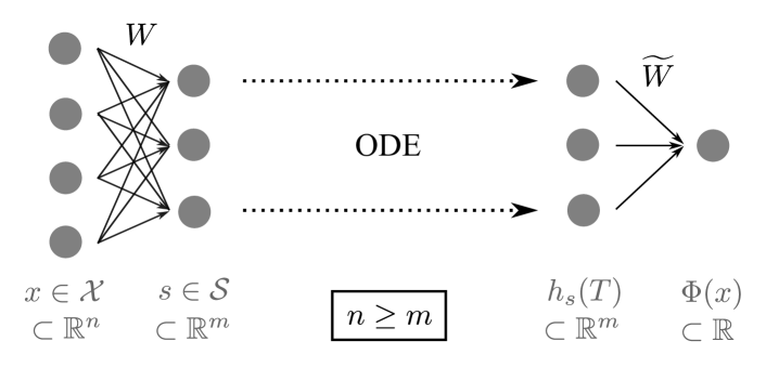
(a) Structure of a non-augmented neural ODE $\Phi\in\text{NODE}_{\textup{N}}^{k}(\mathcal{X},\mathbb{R})$, $W$ and $\widetilde{W}$ have full rank.

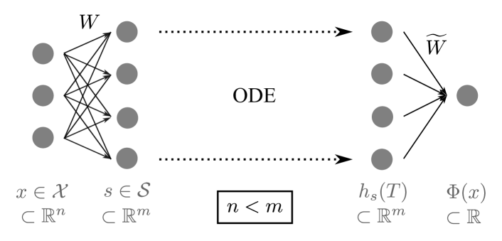
(b) Structure of an augmented neural ODE $\Phi\in\text{NODE}_{\textup{A}}^{k}(\mathcal{X},\mathbb{R})$, $W$ and $\widetilde{W}$ have full rank.

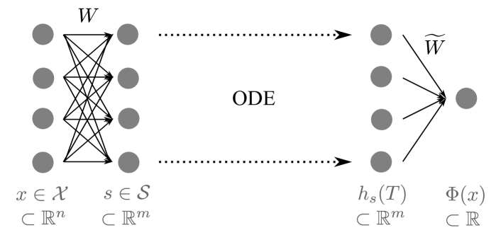
(c) Structure of a neural network with a bottleneck $\Phi\in\text{NODE}_{\textup{B}}^{k}(\mathcal{X},\mathbb{R})$, where at least one of the weight matrices $W$ or $\widetilde{W}$ has not full rank. There is no relationship between the dimensions $m$ and $n$.

Figure 4.1: The three different types of architectures non-augmented, augmented and bottleneck for classical feed-forward neural networks $\Phi\in\text{NODE}^{k}(\mathcal{X},\mathbb{R})$.

Proposition 4.4.

The subdivision of neural ODEs in non-augmented neural ODEs of the form $\textup{NODE}^{k}_{\textup{N}}(\mathcal{X},\mathbb{R})$, augmented neural ODEs of the form $\textup{NODE}^{k}_{\textup{A}}(\mathcal{X},\mathbb{R})$ and neural ODEs with a bottleneck $\textup{NODE}^{k}_{\textup{B}}(\mathcal{X},\mathbb{R})$, is a complete partition in three disjoint sub-classes of neural ODEs, i.e.

$$\textup{NODE}^{k}(\mathcal{X},\mathbb{R})=\textup{NODE}^{k}_{\textup{N}}(\mathcal{X},\mathbb{R})\;\dot{\cup}\;\,\textup{NODE}^{k}_{\textup{A}}(\mathcal{X},\mathbb{R})\;\dot{\cup}\;\,\textup{NODE}^{k}_{\textup{B}}(\mathcal{X},\mathbb{R}).$$

Proof.

All scalar neural ODEs of the form $\textup{NODE}^{k}(\mathcal{X},\mathbb{R})$ can be split up in neural ODEs, where the weight matrices $W$ and $\widetilde{W}$ have both full rank or at least one weight matrix has not full rank and hence the neural ODE is of class $\textup{NODE}^{k}_{\textup{B}}(\mathcal{X},\mathbb{R})$. The neural ODEs with full rank matrices are subdivided in the classes $\textup{NODE}^{k}_{\textup{N}}(\mathcal{X},\mathbb{R})$ and $\textup{NODE}^{k}_{\textup{A}}(\mathcal{X},\mathbb{R})$, depending on if $n\geq m$ or if $n<m$, such that we obtain a complete partition in three disjoint sub-classes of neural ODEs. ∎

Remark 4.5.

The comparison of non-augmented and augmented neural ODEs with classical feed-forward neural networks with full rank matrices is straightforward. Neural ODEs with a bottleneck resemble neural networks with a bottleneck in the following sense: if $\textup{rank}(W)=r<\min\{m,n\}$, then $L(x)$ has $r$ linearly independent components, such that the effective dimension of the input is reduced from $n$ to $r$. As the ODE lives in $\mathbb{R}^{m}$, the dimension is increased from $r$ to $m$, inducing a hidden bottleneck as $n>r$ and $r<m$. In the case that $\textup{rank}(\widetilde{W})=0$, the output of the neural ODE is constant and has no non-trivial dynamics.

For the upcoming analysis, we define in analogy to classical feed-forward neural networks a weight space for the weight matrices and biases of scalar neural ODEs. For neural ODEs, the vector field $f$, which corresponds to all weights, biases and activation functions of the hidden layer of a feed-forward neural network, can be freely chosen. As our results do not depend on the choice of the vector field $f$, we define in the following only a weight space for the weights and biases $W$, $\widetilde{W}$, $b$ and $\tilde{b}$.

Definition 4.6.

Let $\Phi\in\textup{NODE}^{k}(\mathcal{X},\mathbb{R})$ be a scalar neural ODE with weight matrices $W\in\mathbb{R}^{m\times n}$, $\widetilde{W}\in\mathbb{R}^{1\times m}$ and biases $b\in\mathbb{R}^{m}$, $\tilde{b}\in\mathbb{R}$. The weight spaces $\mathbb{V}$ of all possible weights is defined as

$$\mathbb{V}\coloneqq\mathbb{R}^{m\times n}\times\mathbb{R}^{1\times m}\times\mathbb{R}^{m}\times\mathbb{R}$$

The set of stacked weights, where the matrices $W$ and $\widetilde{W}$ have full rank, is a subset of $\mathbb{R}^{N_{V}}$, $N_{V}\coloneqq mn+2m+1$, defined by

$$\mathbb{V}^{\ast}\coloneqq\left\{(\textup{vec}(W);\widetilde{W}^{\top};b;\tilde{b})\in\mathbb{R}^{N_{V}}:\textup{rank}(W)=\min\{m,n\}\wedge\textup{rank}(\widetilde{W}=1)\right\},$$

with the operator vec of Definition 3.4.

By definition, it holds that the weight matrices of non-augmented and augmented neural ODEs lie in $\mathbb{V}^{\ast}$ and the weight matrices of neural ODEs with a bottleneck lie in $\mathbb{R}^{N_{V}}\setminus\mathbb{V}^{\ast}$. As for feed-forward neural networks it also holds for neural ODEs that the set of weights $\mathbb{R}^{N_{V}}\setminus\mathbb{V}^{\ast}$, where at least one weight matrix has not full rank, is a set of Lebesgue measure zero in $\mathbb{R}^{N_{V}}$.

Lemma 4.7.

The set $\mathbb{R}^{N_{V}}\setminus\mathbb{V}^{\ast}$ is a zero set w.r.t. the Lebesgue measure in $\mathbb{R}^{N_{V}}$.

Proof.

Let $(W,\widetilde{W},b,\tilde{b})\in\mathbb{V}$. By Lemma 3.6, the set

$$W_{0}\coloneqq\left\{\textup{vecm}(W,\widetilde{W})\in\mathbb{R}^{mn+m}:\textup{rank}(W)<\min\{m,n\}\vee\textup{rank}(\widetilde{W})=0\right\}$$

is a zero set w.r.t the Lebesgue measure in $\mathbb{R}^{mn+m}$. It follows that also the set

$$W_{0}\times\mathbb{R}^{m}\times\mathbb{R}=\mathbb{R}^{N_{V}}\setminus\mathbb{V}^{\ast}$$

is a zero set w.r.t the Lebesgue measure in $\mathbb{R}^{N_{V}}$. ∎

4.2 Existence of Critical Points

In this section, we study the existence of critical points dependent on the special architecture of the scalar neural ODE. As for feed-forward neural networks, we first calculate the network gradient.

Lemma 4.8.

Let $\Phi\in\textup{NODE}^{k}(\mathcal{X},\mathbb{R})$, $k\geq 1$, $\mathcal{X}\subset\mathbb{R}^{n}$, be a scalar neural ODE with weight matrices $(W,\widetilde{W},b,\tilde{b})\in\mathbb{V}$. Then

$$\nabla\Phi(x)=W^{\top}\left(\frac{\partial h_{s}(T)}{\partial s}\right)^{\top}\widetilde{W}^{\top}\in\mathbb{R}^{n},$$

where $s=Wx+b$ and $\frac{\partial h_{s}(T)}{\partial s}\in\mathbb{R}^{m\times m}$ is the Jacobian matrix of the time-$T$ map $h_{s}(T)$ w.r.t. the initial value $s$ of the ODE, i.e. : $\left[\frac{\partial h_{s}(T)}{\partial s}\right]_{ij}=\frac{\partial[h_{s}(T)]_{i}}{\partial s_{j}}$.

Proof.

By Lemma 4.2 it holds $\Phi\in C^{1}(\mathcal{X},\mathbb{R})$, such that the multi-dimensional chain rule applied to

$$\Phi(x)\coloneqq\widetilde{L}(h_{L(x)}(T))=\widetilde{W}\cdot h_{Wx+b}(T)+\tilde{b}=\widetilde{W}\cdot h_{s}(T)+\tilde{b}$$

yields

$$\frac{\mathrm{d}\Phi}{\mathrm{d}x}=\widetilde{W}\frac{\partial h_{s}(T)}{\partial s}W\in\mathbb{R}^{1\times n}$$

where $s=Wx+b$. The result follows by taking the transpose. ∎

To determine if a neural ODE has critical points, we need to characterize the Jacobian matrix $\frac{\partial h_{s}(T)}{\partial s}$. To that purpose, we need the following two results from ODE theory.

Lemma 4.9 ([8]).

Let $f\in C^{k,0}(\mathbb{R}^{m}\times\mathcal{I},\mathbb{R}^{m})$ with $k\geq 1$. Then the solution $h_{s}(t)$ of the initial value problem (IVP) is continuously differentiable w.r.t. the initial condition $s\in\mathcal{S}$ and the Jacobian matrix $\frac{\partial h_{s}(t)}{\partial s}\in\mathbb{R}^{m\times m}$ satisfies the linear variational equation

$$\frac{\mathrm{d}Y}{\mathrm{d}t}=\frac{\partial f(h_{s}(t),t)}{\partial h_{s}}Y,$$

with $Y(t)\in\mathbb{R}^{m\times m}$ and initial condition $\frac{\partial h_{s}(0)}{\partial s}=\textup{Id}_{m}$, where $\textup{Id}_{m}\in\mathbb{R}^{m\times m}$ is the identity matrix. The matrix $\frac{\partial f(h_{s}(t),t)}{\partial h_{s}}\in\mathbb{R}^{m\times m}$ is the Jacobian of the vector field $f(h_{s}(t),t)$ w.r.t. $h_{s}$, defined by $\left[\frac{\partial f(h_{s}(t),t)}{\partial h_{s}}\right]_{ij}=\frac{\partial[f(h_{s}(t),t)]_{i}}{\partial[h_{s}]_{j}}$.

Lemma 4.10 ([3]).

Consider the linear homogeneous ODE

$$\frac{\mathrm{d}y}{\mathrm{d}t}=A(t)y,$$ (4.2)

where $y\in\mathbb{R}^{m}$ and $A\in C^{0}(\mathcal{I},\mathbb{R}^{m\times m})$, $\mathcal{I}\subset\mathbb{R}$ open, is continuous.

1. Given an initial condition $y(t_{0})=y_{0}$, $t_{0}\in\mathcal{I}$, then (4.2) has a unique solution $y:\mathcal{I}\rightarrow\mathbb{R}^{m}$.

2. If $Y:\mathcal{I}\rightarrow\mathbb{R}^{m\times m}$ is a matrix solution of (4.2) with initial condition $Y(t_{0})=Y_{0}\in\mathbb{R}^{m\times m}$, i.e. every column $[Y]_{i}\in\mathbb{R}^{m}$, $i\in\{1,\ldots,m\}$ is a solution of  (4.2) with initial condition $[Y]_{i}(0)=[Y_{0}]_{i}\in\mathbb{R}^{m}$, then Liouville’s formula holds:

   $$\det(Y(t))=\det(Y(t_{0}))\exp\left(\int_{t_{0}}^{t}\textup{tr}(A(r))\;\mathrm{d}r\right),$$

   where $\textup{tr}(A(r))$ is the trace of the matrix $A\in C^{0}(\mathcal{I},\mathbb{R}^{m\times m})$.

With these two lemmas, we can prove that the Jacobian matrix $\frac{\partial h_{s}(T)}{\partial s}$ has independently of the choice of the vector field $f$ and the initial condition $s$ always full rank.

Proposition 4.11.

Let $\Phi\in\textup{NODE}(\mathcal{X},\mathbb{R})$. Then the Jacobian $\frac{\partial h_{s}(T)}{\partial s}$ of the time-$T$ map $h_{s}(T)$ w.r.t the initial data $s\in\mathcal{S}=L(\mathcal{X})$ of the underlying initial value problem (IVP) has always full rank $m$.

Proof.

As $k\geq 1$, the initial value problem (IVP) with initial condition $s\in\mathcal{S}=L(\mathcal{X})$ has by Lemma 4.1 a unique solution $h_{s}:\mathcal{I}\rightarrow\mathbb{R}^{m}$ with $[0,T]\subset\mathcal{I}$, $\mathcal{I}\subset\mathbb{R}$ open. Furthermore, given the continuously differentiable solution $h_{s}:\mathcal{I}\rightarrow\mathbb{R}^{m}$ of (IVP), the matrix function $A:\mathcal{I}\rightarrow\mathbb{R}^{m\times m}$, $A(t)\coloneqq\frac{\partial f(h_{s}(t),t)}{\partial h_{y}}$, is continuous. By Lemma 4.9, the Jacobian matrix $\frac{\partial h_{s}(t)}{\partial s}\in\mathbb{R}^{m\times m}$ satisfies the linear homogeneous ODE

$$\frac{\mathrm{d}Y}{\mathrm{d}t}=A(t)Y,\qquad Y(0)=\text{Id}_{m},$$

where $\text{Id}_{m}\in\mathbb{R}^{m\times m}$ is the identity matrix. By Lemma 4.10(a), each column of $Y$ defines a unique solution $[Y]_{i}:\mathcal{I}\rightarrow\mathbb{R}^{m}$ with initial condition $[Y]_{i}(0)=\mathrm{e}_{i}^{(m)}$, where $\mathrm{e}_{i}^{(m)}$ is the $i$-th unit vector in $\mathbb{R}^{m}$. Hence, $Y:\mathcal{I}\rightarrow\mathbb{R}^{m\times m}$ is a unique matrix solution defined for all $t\in[0,T]\subset\mathcal{I}$ with initial condition $Y(0)=\text{Id}_{m}$, such that $\det(Y(0))=1$. As the matrix $A(t)\in\mathbb{R}^{m\times m}$ has only real entries, all eigenvalues of $A(t)$ are real or they come in complex conjugate pairs, such that the trace of $A(t)$ is a real number for all $t\in\mathcal{I}$. Consequently,

$$\exp\left(\int_{t_{0}}^{t}\textup{tr}(A(r))\;\mathrm{d}r\right)$$

is a real-valued, positive number, such that it follows by Lemma 4.10(b) that $\det(Y(T))\neq 0$. Consequently $Y(T)=\frac{\partial h_{s}(T)}{\partial s}$ has full rank $m$, independently of the initial data $s\in\mathcal{S}$. ∎

The characterization of the Jacobian matrix $\frac{\partial h_{s}(T)}{\partial s}$ in Proposition 4.11 is sufficient to prove that for non-augmented scalar ODEs, no critical points can exist.

Theorem 4.12.

Any non-augmented scalar neural ODE $\Phi\in\textup{NODE}_{\textup{N}}(\mathcal{X},\mathbb{R})$, $k\geq 1$ has no critical point, i.e. $\nabla\Phi(x)\neq 0$ for all $x\in\mathcal{X}$. Consequently it holds for $k\geq 1$ that

$$\textup{NODE}_{\textup{N}}(\mathcal{X},\mathbb{R})\subset(\mathcal{C}1)^{k}(\mathcal{X},\mathbb{R}),$$

such that every non-augmented scalar neural ODE is a Morse function.

Proof.

Denote the weight matrices of $\Phi$ by $(W,\widetilde{W},b,\tilde{b})\in\mathbb{V}$. By Lemma 4.8 it holds

$$\nabla\Phi(x)=W^{\top}\left(\frac{\partial h_{s}(T)}{\partial s}\right)^{\top}\widetilde{W}^{\top}\in\mathbb{R}^{n}.$$

As the neural ODE is non-augmented, $W^{\top}\in\mathbb{R}^{n\times m}$ has rank $m\leq n$ and $\widetilde{W}^{\top}\in\mathbb{R}^{m\times 1}$ has rank 1. By Proposition 4.11, the Jacobian $\left(\frac{\partial h_{s}(T)}{\partial s}\right)^{\top}\in\mathbb{R}^{m\times m}$ has independently of $s\in\mathcal{S}$ and hence also independently of $x\in\mathcal{X}$ full rank $m\geq 1$. By Lemma 3.10, the product $\nabla\Phi(x)$ of the three given full rank matrices with monotonically decreasing widths has also full rank $1$, which implies that $\nabla\Phi(x)\neq 0$ for all $x\in\mathcal{X}$ and the result follows. ∎

Remark 4.13.

Theorem 4.12 generalizes the results obtained in [15], where it is shown that a non-augmented neural ODE with $n=m$ and $W=\textup{Id}_{n}$ cannot be of class $(\mathcal{C}2)^{k}(\mathcal{X},\mathbb{R})$.

The following theorem shows, that the proof of Theorem 4.12 does not apply for augmented and bottleneck neural ODEs. It guarantees the existence of neural ODE architectures $\Phi\in\textup{NODE}_{\textup{A}}(\mathcal{X},\mathbb{R})$ and $\Phi\in\textup{NODE}_{\textup{B}}(\mathcal{X},\mathbb{R})$, which do have critical points.

Theorem 4.14.

Let $f\in C^{k,0}(\mathbb{R}^{m}\times\mathcal{I},\mathbb{R}^{m})$, $k\geq 1$ be a vector field, such that $[0,T]\subset\mathcal{I}$ for the initial value problem (IVP).

1. Given $W\in\mathbb{R}^{n\times m}$ with $n<m$ and $\textup{rank}(W)=n$ and a point $x\in\mathcal{X}$, then the weight matrix $\widetilde{W}\in\mathbb{R}^{1\times m}$ can be chosen in such a way, that $\Phi\in\textup{NODE}_{\textup{A}}(\mathcal{X},\mathbb{R})$ has a critical point at $x$.

2. Given $W\in\mathbb{R}^{n\times m}$ with $\textup{rank}(W)<\min\{m,n\}$ and a point $x\in\mathcal{X}$, then the weight matrix $\widetilde{W}\in\mathbb{R}^{1\times m}$ can be chosen in such a way, that $\Phi\in\textup{NODE}_{\textup{B}}(\mathcal{X},\mathbb{R})$ has a critical point at $x$.

Proof.

By Lemma 4.8 it holds

$$\nabla\Phi(x)=W^{\top}\left(\frac{\partial h_{s}(T)}{\partial s}\right)^{\top}\widetilde{W}^{\top}\in\mathbb{R}^{n},$$

where $s=Wx+b$ for the given $x\in\mathcal{X}$. The Jacobian $\frac{\partial h_{s}(T)}{\partial s}$ has by Lemma 4.11 full rank $m$.

In case (a), the matrix product $W^{\top}\left(\frac{\partial h_{s}(T)}{\partial s}\right)^{\top}\in\mathbb{R}^{n\times m}$ has by Lemma 3.10 full rank $n<m$, which implies that the $m$ columns of the matrix product are linearly dependent. Hence, there exists a non-zero choice of the matrix $\widetilde{W}\in\mathbb{R}^{1\times m}$, such that $\nabla\Phi(x)=0$ for the given $x\in\mathcal{X}$.

In case (b), the matrix $W$ has non-full rank, i.e. $\text{rank}(W)=r<\min\{m,n\}$. As the Jacobian matrix $\frac{\partial h_{s}(T)}{\partial s}$, has full rank, it follows that the matrix product $W^{\top}\left(\frac{\partial h_{s}(T)}{\partial s}\right)^{\top}\in\mathbb{R}^{n\times m}$ has also rank $r$. Since $r<\min\{m,n\}$, the $m$ columns of the matrix product are linearly dependent. Hence, there exists a non-zero choice of the matrix $\widetilde{W}\in\mathbb{R}^{1\times m}$, such that $\nabla\Phi(x)=0$ for the given $x\in\mathcal{X}$. ∎

4.3 Regularity of Critical Points

For a further characterization of augmented and bottleneck neural ODEs, we study the regularity of the critical points. A first observation already made in [15] and [28], is that an augmentation of the phase space in combination with a linear layer is sufficient, to represent any function exactly. In our setting this means, that for any map $\Psi\in C^{k}(\mathcal{X},\mathbb{R})$, $k\geq 0$, there exists an augmented scalar neural ODE $\Phi\in\text{NODE}^{k}(\mathcal{X},\mathbb{R})$ such that $\Psi(x)=\Phi(x)$ for all $x\in\mathcal{X}$.

Theorem 4.15.

Any map $\Psi\in C^{k}(\mathcal{X},\mathbb{R})$, $k\geq 0$, $\mathcal{X}\subset\mathbb{R}^{n}$ can be exactly represented by an augmented scalar neural ODE $\Phi\in\textup{NODE}^{k}_{\textup{A}}(\mathcal{X},\mathbb{R})$ with arbitrary $m>n$, i.e. $\Psi(x)=\Phi(x)$ for all $x\in\mathcal{X}$.

Proof.

In analogy to the proof in [14], we fix $T>0$, choose $m>n$ and define the augmented neural ODE $\Phi$ by the weights

$$W=\begin{pmatrix}\textup{Id}_{n}\\ 0\end{pmatrix}\in\mathbb{R}^{m\times n},\quad b=0\in\mathbb{R}^{m},\quad\widetilde{W}=(0,\ldots,0,1)\in\mathbb{R}^{1\times m},\quad\tilde{b}=0\in\mathbb{R}$$

and the ODE

$$\frac{\mathrm{d}}{\mathrm{d}t}\begin{pmatrix}h_{1}\\ \vdots\\ h_{m-1}\\ h_{m}\end{pmatrix}=\begin{pmatrix}0\\ \vdots\\ 0\\ \frac{1}{T}\cdot\Psi(h_{1},\ldots.h_{n})\end{pmatrix}\eqqcolon f(h_{1},\ldots,h_{n},t),$$

such that the vector field $f$ is of class $C^{k,0}(\mathcal{X}\times\mathbb{R},\mathbb{R})$. $\Phi$ is augmented, as $m>n$ and the weights matrices $W$ and $\widetilde{W}$ have full rank. By Lemma 4.2 it holds $\Phi\in\textup{NODE}^{k}_{\textup{A}}(\mathcal{X},\mathbb{R})$ and it follows

$$\Phi(x)=\widetilde{W}\cdot h_{Wx+b}(T)+\tilde{b}=\widetilde{W}\cdot h_{(x,0)^{\top}}(T)=\widetilde{W}\begin{pmatrix}x\\ 0\\ \Psi(x)\end{pmatrix}=\Psi(x)$$

for all $x\in\mathcal{X}$. ∎

The last theorem implies, that any function $\Psi\in C^{k}(\mathcal{X},\mathbb{R})$, $k\geq 0$ can be represented exactly by an augmented neural ODE. If $k\geq n+1\geq 2$, Morse functions are by Theorem 2.2 a dense subset in the Banach space of $k$ times differentiable functions. Theorem 4.15 does not characterize, if Morse functions are also dense in the space of augmented neural ODEs, i.e. if it is a generic property of a map $\Phi\in\textup{NODE}^{k}_{\textup{A}}(\mathcal{X},\mathbb{R})$ to be a Morse function. In analogy to classical feed-forward neural networks, we show in the following that this is the case for all weights, except possibly for a zero set with respect to the Lebesgue measure.

Theorem 4.16.

Any augmented scalar neural ODE $\Phi\in\textup{NODE}^{k}_{\textup{A}}(\mathcal{X},\mathbb{R})$, $k\geq 2$ is for all weights $(\textup{vec}(W);\widetilde{W}^{\top};b;\tilde{b})\in\mathbb{V}^{\ast}$, except possibly for a zero set in $\mathbb{R}^{N_{V}}$ w.r.t. the Lebesgue measure, of class $(\mathcal{C}1)^{k}(\mathcal{X},\mathbb{R})$ or $(\mathcal{C}2)^{k}(\mathcal{X},\mathbb{R})$ and hence a Morse function.

Proof.

Let $\Phi\in\textup{NODE}^{k}_{\textup{A}}(\mathcal{X},\mathbb{R})$ be an augmented scalar neural ODE with full rank weight matrices $W\in\mathbb{R}^{m\times n}$, $\widetilde{W}\in\mathbb{R}^{1\times m}$ and biases $b\in\mathbb{R}^{n}$, $\tilde{b}\in\mathbb{R}$. By Theorem 4.14(a) it is possible that the neural ODE $\Phi$ has a critical point. In the case that $\Phi$ has no critical point, $\Phi$ is of class $(\mathcal{C}1)^{k}(\mathcal{X},\mathbb{R})$ and hence a Morse function. In the following we show, that if $\Phi$ has a critical point, then it is for all weights, where $\Phi$ has critical points, except possibly for a zero set w.r.t. the Lebesgue measure in $\mathbb{R}^{N_{V}}$ of class $(\mathcal{C}2)^{k}(\mathcal{X},\mathbb{R})$. By Lemma 4.8, the gradient of $\Phi$ is given by

$$\nabla\Phi(x)=W^{\top}\left(\frac{\partial h_{s}(T)}{\partial s}\right)^{\top}\widetilde{W}^{\top}\in\mathbb{R}^{n},$$

where $s=Wx+b$ and $\frac{\partial h_{s}(T)}{\partial s}\in\mathbb{R}^{m\times m}$ is the Jacobian matrix of the time-$T$ map $h_{s}(T)$ w.r.t. the initial value $s$. For a weight vector $v\in\mathbb{V}^{\ast}$, we define $\widehat{\Phi}\in C^{k}(\mathcal{X}\times\mathbb{V}^{\ast})$, $k\geq 2$, to be the neural ODE $\Phi$ with an explicit dependence on the weight vector $v$. As a composition of $k$ times continuously differentiable functions, $\widehat{\Phi}$ is not only in $x$ but also in $v$ $k$ times continuously differentiable. We aim to apply Lemma 3.23 to show that $\Phi$ is for all weights $v\in\mathbb{V}^{\ast}$, except possibly for a set of measure zero w.r.t. the Lebesgue measure in $\mathbb{R}^{N_{V}}$ a Morse function. To that purpose, we need to show that the matrix $\frac{\partial^{2}\widehat{\Phi}}{\partial v\partial x}\in\mathbb{R}^{n\times p}$ has for every $(x,v)\in\mathcal{X}\times\mathbb{V}^{\ast}$ full rank. The second partial derivatives with respect to $x$ and the components of $\widetilde{W}$ are given by

$$\frac{\partial^{2}\widehat{\Phi}}{\partial[\widetilde{W}]_{i}\partial x}=\frac{\partial}{\partial[\widetilde{W}]_{i}}\left[W^{\top}\left(\frac{\partial h_{s}(T)}{\partial s}\right)^{\top}\widetilde{W}^{\top}\right]=W^{\top}\left(\frac{\partial h_{s}(T)}{\partial s}\right)^{\top}\mathrm{e}_{i}^{(m)},$$

where $\mathrm{e}_{i}^{(m)}$ denotes the $i$-th unit vector in $\mathbb{R}^{m}$. Consequently it follows that

$$\frac{\partial^{2}\widehat{\Phi}}{\partial\widetilde{W}\partial x}=W^{\top}\left(\frac{\partial h_{s}(T)}{\partial s}\right)^{\top}\in\mathbb{R}^{n\times m},$$

has full rank $n$, since by assumption the matrix $W$ has full rank $n$ as $m>n$ and by Proposition 4.11 the Jacobian $\frac{\partial h_{s}(T)}{\partial s}$ has full rank $m$. Hence, the weight matrix $\frac{\partial^{2}\widehat{\Phi}}{\partial v\partial x}\in\mathbb{R}^{n\times p}$ has for every $(x,v)\in\mathcal{X}\times\mathbb{V}^{\ast}$ full rank $n<p$, because the submatrix $\frac{\partial^{2}\widehat{\Phi}}{\partial\widetilde{W}\partial x}$ has rank $n$. Lemma 3.23 implies, that $\Phi$ is for all weights $v\in\mathbb{V}^{\ast}$, except possibly for a zero set w.r.t. the Lebesgue measure in $\mathbb{R}^{N_{V}}$ a Morse function. ∎

We illustrate the assertion of the last theorem in a one-dimensional example.

Example 4.17.

Consider the scalar augmented neural ODE $\Phi\in\textup{NODE}^{\infty}_{\textup{A}}(\mathbb{R},\mathbb{R})$ with $n=1$, $m=2$ defined by the weights and biases

$$W=\begin{pmatrix}w_{1}\\ w_{2}\end{pmatrix}\in\mathbb{R}^{2},\qquad b=\begin{pmatrix}b_{1}\\ b_{2}\end{pmatrix}\in\mathbb{R}^{2},\qquad\widetilde{W}=(\widetilde{w}_{1},\widetilde{w}_{2})\in\mathbb{R}^{1\times 2},\qquad\tilde{b}\in\mathbb{R},$$

which is visualized in Figure 4.2. As underlying initial value problem we consider

$$\frac{\mathrm{d}}{\mathrm{d}t}\begin{pmatrix}h_{1}\\ h_{2}\end{pmatrix}=\begin{pmatrix}0\\ \exp(h_{1})\end{pmatrix},\qquad\begin{pmatrix}h_{1}(0)\\ h_{2}(0)\end{pmatrix}=Wx+b,$$

with solution

$$\begin{pmatrix}h_{1}(t)\\ h_{2}(t)\end{pmatrix}=\begin{pmatrix}w_{1}x+b_{1}\\ w_{2}x+b_{2}+\exp(w_{1}x+b_{1})t\end{pmatrix},$$

such that it follows

$$\Phi(x) =\tilde{w}_{1}(w_{1}x+b_{1})+\tilde{w}_{2}(w_{2}x+b_{2}+\exp(w_{1}x+b_{1})T),$$

$$\nabla\Phi(x) =\tilde{w}_{1}w_{1}+\tilde{w}_{2}w_{2}+\tilde{w}_{2}w_{1}\exp(w_{1}x+b_{1})T,$$

$$H_{\Phi}(x) =\tilde{w}_{2}w_{1}^{2}\exp(w_{1}x+b_{1})T.$$

Consequently, $\Phi$ can only be of class $(C3)^{\infty}(\mathbb{R},\mathbb{R})$ if

$$(\textup{vec}(W);\widetilde{W}^{\top};b;\tilde{b})\in\left\{(w_{1},w_{2},\tilde{w}_{1},\tilde{w}_{2},b_{1},b_{2},\tilde{b})\in\mathbb{V}^{\ast}\subset\mathbb{R}^{7}:\tilde{w}_{2}=0\vee w_{1}=0\right\},$$

which is a zero set w.r.t. the Lebesgue measure in $\mathbb{R}^{7}$. Hence for all weights $(\textup{vec}(W);\widetilde{W}^{\top};b;\tilde{b})\in\mathbb{V}^{\ast}$, except possibly for a zero set in $\mathbb{R}^{7}$ w.r.t. the Lebesgue measure, $\Phi$ is of class $(\mathcal{C}1)^{k}(\mathcal{X},\mathbb{R})$ or $(\mathcal{C}2)^{k}(\mathcal{X},\mathbb{R})$.

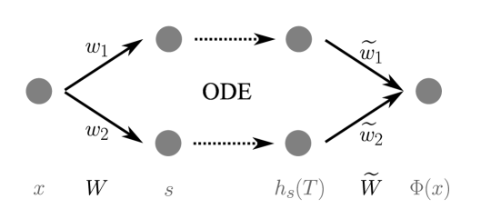
Figure 4.2: Scalar augmented neural ODE $\Phi\in\textup{NODE}^{\infty}_{\textup{A}}(\mathbb{R},\mathbb{R})$ of Example 4.17.

For neural ODEs with a bottleneck, we cannot guarantee that the considered matrix $\frac{\partial^{2}\widehat{\Phi}}{\partial v\partial x}$ in the proof of Theorem 4.16 has always full rank. In the following we can directly show, that any critical point of a neural ODE with a bottleneck has to be degenerate. To that purpose, we derive a formula for the Hessian matrix $H_{\Phi}(x)$.

Lemma 4.18.

Let $\Phi\in\textup{NODE}^{k}(\mathcal{X},\mathbb{R})$, $k\geq 2$, $\mathcal{X}\subset\mathbb{R}^{n}$ be a scalar neural ODE with weight matrices $(W,\widetilde{W},b,\tilde{b})\in\mathbb{V}$. Then

$$H_{\Phi}(x)=W^{\top}H_{\eta}(s)W\in\mathbb{R}^{n\times n},$$

where $s=L(x)=Wx+b$ and $\eta\in C^{k}(\mathcal{S},\mathbb{R})$, $\eta(s)\coloneqq\widetilde{W}h_{s}(T)$, $\mathcal{S}=L(\mathcal{X})$.

Proof.

We introduce $\eta:\mathcal{S}\rightarrow\mathbb{R}$, $\eta(s)\coloneqq\widetilde{W}h_{s}(T)$, which is by Lemma 4.1 of class $C^{k}(\mathcal{S},\mathbb{R})$ with $\mathcal{S}=L(\mathcal{X})$. It follows

$$\nabla\eta(x)=\frac{\partial h_{s}(T)}{\partial s}^{\top}\widetilde{W}^{\top}\in\mathbb{R}^{m},$$

such that Lemma 4.8 implies $\nabla\Phi(x)=W^{\top}\nabla\eta(x)$. Hence, the multi-dimensional chain rule implies

$$H_{\Phi}(x)=\nabla(\nabla\Phi(x)^{\top})=\nabla(\nabla\eta(x)^{\top}W)=W^{\top}H_{\eta}(s)W\in\mathbb{R}^{n\times n},$$

where $s=Wx+b$. ∎

Without any analysis of the Hessian matrix $H_{\eta}$, we can directly conclude, that every critical point of a neural ODE with a bottleneck is degenerate, as at least one of the weight matrices $W$ or $\widetilde{W}$ is singular.

Theorem 4.19.

Any scalar neural ODE with a bottleneck $\Phi\in\textup{NODE}^{k}_{\textup{B}}(\mathcal{X},\mathbb{R})$ has only degenerate critical points, i.e. $\Phi$ is of class $(\mathcal{C}1)^{k}(\mathcal{X},\mathbb{R})$ or $(\mathcal{C}3)^{k}(\mathcal{X},\mathbb{R})$.

Proof.

As the scalar neural ODE $\Phi$ has a bottleneck, at least one of the weight matrices $W\in\mathbb{R}^{m\times n}$ and $\widetilde{W}\in\mathbb{R}^{1\times m}$ has not full rank. If $\widetilde{W}=0$, then $\Phi(x)=\tilde{b}$ is constant, such that every point $x\in\mathcal{X}$ is a degenerate critical point and hence $\Phi\in(\mathcal{C}3)^{k}(\mathcal{X},\mathbb{R})$. If $\textup{rank}(W)<\min\{m,n\}$, then it holds

$$\textup{rank}(H_{\Phi}(x))\leq\min\{\textup{rank}(W^{\top}),\textup{rank}(H_{\eta}(s)),\textup{rank}(W)\}<\min\{m,n\},$$

which implies that the Hessian matrix $H_{\Phi}(x)$ is singular. Consequently if $\Phi$ has a critical point, then $\Phi\in(\mathcal{C}3)^{k}(\mathcal{X},\mathbb{R})$ and if $\Phi$ has no critical point, then $\Phi\in(\mathcal{C}1)^{k}(\mathcal{X},\mathbb{R})$. ∎

In Theorem 3.28 we showed, that feed-forward neural networks with a bottleneck can be of all classes $(\mathcal{C}1)^{k}(\mathcal{X},\mathbb{R})$, $(\mathcal{C}2)^{k}(\mathcal{X},\mathbb{R})$ and $(\mathcal{C}3)^{k}(\mathcal{X},\mathbb{R})$. The following remark explains, why nevertheless, the results established for neural networks and neural ODEs are comparable.

Remark 4.20.

It is for both scalar neural ODEs and feed-forward neural networks the case that if the last layer $\widetilde{W}\in\mathbb{R}^{1\times m}$ or $\widetilde{W}_{L}\in\mathbb{R}^{1\times m_{L}}$ has not full rank, the output is constant and hence the network is of class $(C3)^{k}(\mathcal{X},\mathbb{R})$. We can compare the case that the weight matrix $W\in\mathbb{R}^{m\times n}$ of the neural ODE has not full rank with the case, that the first weight matrix $W_{1}\in\mathbb{R}^{m_{1}\times n}$ of the feed-forward neural network has not full rank. If $W_{1}$ is singular, still all four types of bottlenecks in Theorem 3.28 are possible, but Theorem  3.15 implies, that the neural network cannot be of class $(\mathcal{C}2)^{k}(\mathcal{X},\mathbb{R})$. This is the case, as a linear change of coordinates to obtain an equivalent neural network architecture is by the proof of Theorem 3.12 needed if and only if the first weight matrix $W_{1}$ has not full rank. The difference of the results of neural ODEs and feed-forward neural networks is induced by the fact, that for neural ODEs the bottleneck obstruction cannot occur in the initial value problem, which corresponds to the hidden layer of the neural network.

For the more interesting case, that the first weight matrix $W\in\mathbb{R}^{m\times n}$ of the scalar neural ODE has not full rank, we provide an example which illustrates that the neural ODE can be both of class $(\mathcal{C}1)^{k}(\mathcal{X},\mathbb{R})$ or $(\mathcal{C}3)^{k}(\mathcal{X},\mathbb{R})$.

Example 4.21.

Consider the scalar neural ODE with a bottleneck $\Phi\in\textup{NODE}^{k}_{\textup{B}}(\mathbb{R},\mathbb{R})$, $k\geq 2$ with $n=2$, $m=2$ defined by the weights and biases

$$W=\begin{pmatrix}w_{11}&w_{12}\\ w_{21}&w_{22}\end{pmatrix}\in\mathbb{R}^{2\times 2},\qquad b=\begin{pmatrix}b_{1}\\ b_{2}\end{pmatrix}\in\mathbb{R}^{2},\qquad\widetilde{W}=(\widetilde{w}_{1},\widetilde{w}_{2})\in\mathbb{R}^{1\times 2},\qquad\tilde{b}\in\mathbb{R},$$

where we assume that the bottleneck is induced by the condition $\textup{rank}(W)=1$. $\Phi$ is visualized in Figure 4.3. As $\textup{rank}(W)=1$, there exists a constant $\lambda$, such that

$$\begin{pmatrix}w_{21}&w_{22}\end{pmatrix}=\lambda\cdot\begin{pmatrix}w_{11}&w_{12}\end{pmatrix}\qquad\Rightarrow\qquad s=\begin{pmatrix}s_{1}\\ s_{2}\end{pmatrix}=Wx+b=\begin{pmatrix}q+b_{1}\\ \lambda q+b_{2}\end{pmatrix}$$

with $q\coloneqq w_{11}x_{1}+w_{12}x_{2}$. Consequently it holds

$$\Phi(x)=\tilde{w}_{1}[h_{s}(T)]_{1}+\tilde{w}_{2}[h_{s}(T)]_{2}$$

and it follows for the gradient

$$\nabla\Phi(x)=\begin{pmatrix}w_{11}\left(\frac{\partial\Phi}{\partial s_{1}}+\lambda\frac{\partial\Phi}{\partial s_{2}}\right)\\ w_{12}\left(\frac{\partial\Phi}{\partial s_{1}}+\lambda\frac{\partial\Phi}{\partial s_{2}}\right)\end{pmatrix}.$$

As the columns of $\nabla\Phi$ are linearly dependent, also the columns of the Hessian $H_{\Phi}$ are linearly dependent, which implies that every possible critical point of $\Phi$ is degenerate. Dependent on the vector field and on $\lambda$, $\Phi$ has or does not have critical points. As an example we consider the underlying initial value problem defined by

$$\frac{\mathrm{d}}{\mathrm{d}t}\begin{pmatrix}h_{1}\\ h_{2}\end{pmatrix}=\begin{pmatrix}h_{1}\\ h_{2}\end{pmatrix},\qquad\begin{pmatrix}h_{1}(0)\\ h_{2}(0)\end{pmatrix}=\begin{pmatrix}s_{1}\\ s_{2}\end{pmatrix}\qquad\Rightarrow\qquad\begin{pmatrix}h_{1}(T)\\ h_{2}(T)\end{pmatrix}=\begin{pmatrix}s_{1}e^{T}\\ s_{2}e^{T}\end{pmatrix},$$

such that

$$\nabla\Phi(x)=\begin{pmatrix}w_{11}\left(\tilde{w}_{1}+\lambda\tilde{w}_{2}\right)e^{T}\\ w_{12}\left(\tilde{w}_{1}+\lambda\tilde{w}_{2}\right)e^{T}\end{pmatrix}.$$

Hence, for $\lambda=-\frac{\tilde{w}_{1}}{\tilde{w}_{2}}$ or for $W=0$, every point $x\in\mathcal{X}$ is a degenerate critical point and $\Phi$ is of class $(\mathcal{C}3)^{\infty}(\mathcal{X},\mathbb{R})$, otherwise $\Phi$ has no critical point and is of class $(\mathcal{C}1)^{\infty}(\mathcal{X},\mathbb{R})$.

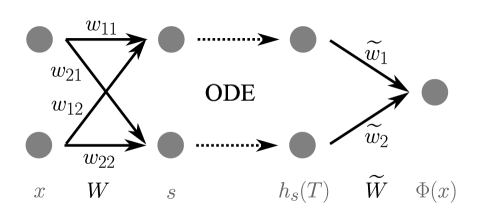
Figure 4.3: Scalar neural ODE with a bottleneck $\Phi\in\textup{NODE}^{k}_{\textup{B}}(\mathbb{R},\mathbb{R})$ of Example 4.21.

5 Conclusion and Outlook

In this work, we studied the geometric structure of the input-output map of feed-forward neural networks and neural ODEs. We used the definition of a Morse function, which is a scalar function, where every critical point is non-degenerate. It is interesting to study the property of being a Morse function, as Morse functions are dense in the space of sufficiently smooth scalar functions and are fundamental building blocks within many areas of mathematics. We fully classified the existence and regularity of critical points depending on the specific architecture of the feed-forward neural network or the neural ODE.

The architectures studied are subdivided in non-augmented, augmented and bottleneck architectures. For classical feed-forward neural networks, the subdivision is defined by width of the largest layer and by checking if there exists a bottleneck in the underlying graph. If at least one weight matrix of a neural network $\Phi$ has not full rank, there exists up to a linear change of coordinates a normal form $\overline{\Phi}$, which is a feed-forward neural network with only full rank matrices and which is equivalent to $\Phi$, i.e. it has the same input-output map. Our proof of the existence of a normal form is constructive, i.e. we gave an explicit algorithm to calculate an equivalent normal form $\overline{\Phi}$. Furthermore we proved that the case that all weight matrices have full rank is generic, i.e. the set of weights, where at least one weight matrix has not full rank has Lebesgue measure zero in the weight space. Hence, we focused in the following analysis on neural networks in normal form.

For neural ODEs, we defined an analogous subdivision in non-augmented, augmented and bottleneck architectures. As neural ODEs can be interpreted as an infinite depth limit of classical feed-forward neural networks, the vector field $f$ of the neural ODE represents all weights, biases and activation functions of the hidden layers. We studied the most general case, where $f$ can be any non-autonomous vector field. In analogy to feed-forward neural networks, the dimension of the phase space defines if an architecture is augmented or non-augmented. We say that a neural ODE has a bottleneck, if at least one of the weight matrices of the linear layers before and after the initial value problem has not full rank.

Our main contribution of this work is to classify in each case the existence and regularity of critical points. In both non-augmented cases, no critical points can exist, as the network gradient has always full rank, which we proved via rank arguments and linear variational equations. If the dimension of at least one layer or the dimension of the phase space is augmented, we showed that it is in both cases possible that critical points exist. Using differential geometry and Morse theory we showed, that except for a zero set with respect to the Lebesgue measure in the weight space, the input-output map is a Morse function. For feed-forward neural networks with a bottleneck, we showed that critical points can be degenerate or non-degenerate. Depending on the dimension of the first bottleneck and the weight matrices, we derived conditions, specifying the regularity of the critical points depending on the type of bottleneck. In contrast to that, we proved for neural ODEs with a bottleneck, that every critical points is degenerate. The different classification for bottleneck architectures relies on the fact, that for neural ODEs the bottleneck cannot occur in the hidden layer. We explain, why nevertheless the results obtained for neural ODEs with a bottleneck are comparable to the results for feed-forward neural networks, where the first weight matrix has not full rank. Overall our results show, that the geometric structure of the input-output map is comparable for feed-forward neural networks and for neural ODEs.

Besides the classification of critical points, we also studied the implications of our results on the universal embedding property of feed-forward neural networks and neural ODEs. For neural ODEs we showed that they cannot have the universal embedding property in the non-augmented and in the bottleneck case, whereas augmented neural ODEs have the universal embedding property. Hereby it was used, that $f$ can be any non-autonomous vector field. In the non-augmented case, feed-forward neural networks cannot have the universal embedding property. For augmented feed-forward neural networks, there exist already various universal approximation theorems in the literature. For the bottleneck case, we distinguished between cases, where no universal embedding is possible, and cases, where the input-output dynamics resembles augmented neural networks, such that it is possible that the neural network has the universal approximation property.

The focus on the exact output of feed-forward neural networks and neural ODEs explains, why certain architectures perform better than others. Our analysis showed, how the dimensions of the layers and the phase space, the rank of the weight matrices, and obstructions such as bottlenecks influence if the input-output map is a Morse function. The established results could be used as a starting point for a perturbation analysis to derive universal approximation results. Furthermore, in future work it would be interesting to study the geometric implications if a feed-forward neural network or a neural ODE is a Morse function. Morse functions are used across many areas, such as topology, differential geometry and data analysis, to study the underlying manifold, on which the Morse function is defined. Transferred to our setting, it is of interest to study the manifold of input data or initial conditions with an augmented neural network defined on it, which is generically a Morse function. Beyond the evident connection to data geometry and its applications, one could even aim to consider from a very theoretical viewpoint, whether neural network representations of Morse functions could be helpful to solve open conjectures in Morse, Morse-Bott and Floer homology.

Acknowledgments: CK and SVK would like to thank the DFG for partial support via the SPP2298 ‘Theoretical Foundations of Deep Learning’. CK would like to thank the VolkswagenStiftung for support via a Lichtenberg Professorship. SVK would like to thank the Munich Data Science Institute (MDSI) for partial support via a Linde doctoral fellowship.

References

- [1] C. C. Aggarwal. Neural Networks and Deep Learning. Springer, 1 edition, 2018. doi:10.1007/978-3-319-94463-0.
- [2] R. T. Q. Chen, Y. Rubanova, J. Bettencourt, and D. Duvenaud. Neural ordinary differential equations. 2018. doi:10.48550/ARXIV.1806.07366.
- [3] C. Chicone. Ordinary Differential Equations with Applications, volume 34 of Texts in Applied Mathematics. Springer New York, 2 edition, 2006. doi:10.1007/0-387-35794-7.
- [4] B. J. Cook, A. D. H. Peterson, W. Woldman, and J. R. Terry. Neural field models: A mathematical overview and unifying framework. Mathematical Neuroscience and Applications, Volume 2, 2022. doi:10.46298/mna.7284.
- [5] C. Esteve, B. Geshkovski, D. Pighin, and E. Zuazua. Large-time asymptotics in deep learning. 2020. doi:10.48550/ARXIV.2008.02491.
- [6] O. Forster. Analysis 2, Differentialrechnung im , gewöhnliche Differentialgleichungen. Grundkurs Mathematik. Springer Spektrum, 11 edition, 2017. doi:10.1007/978-3-658-19411-6.
- [7] J. Guckenheimer and P. Holmes. Nonlinear Oscillations, Dynamical Systems, and Bifurcations of Vector Fields, volume 42 of Applied Mathematical Sciences. Springer New York, 7 edition, 2002. doi:10.1007/978-1-4612-1140-2.
- [8] J. K. Hale. Ordinary Differential Equations. Krieger Publishing Company, 2 edition, 1980.
- [9] K. He, X. Zhang, S. Ren, and J. Sun. Deep residual learning for image recognition. IEEE Conference on Computer Vision and Pattern Recognition, pages 770–778, jun 2016. doi:10.1109/cvpr.2016.90.
- [10] M. W. Hirsch. Differential Topology, volume 33 of Graduate Texts in Mathematics. Springer New York, 1976. doi:10.1007/978-1-4684-9449-5.
- [11] K. Hornik, M. Stinchcombe, and H. White. Multilayer feedforward networks are universal approximators. Neural Networks, 2(5):359–366, jan 1989. doi:10.1016/0893-6080(89)90020-8.
- [12] P. Kidger. On Neural Differential Equations. PhD thesis, Mathematical Institute, University of Oxford, 2022. doi:10.48550/ARXIV.2202.02435.
- [13] A. Kratsios. The universal approximation property - characterization, construction, representation, and existence. Annals of Mathematics and Artificial Intelligence, 89(5-6):435–469, jan 2021. doi:10.1007/s10472-020-09723-1.
- [14] C. Kuehn. PDE Dynamics: An Introduction. Society for Industrial and Applied Mathematics, 2019. doi:10.1137/1.9781611975666.
- [15] C. Kuehn and S.-V. Kuntz. Embedding capabilities of neural ODEs. 2023. doi:10.48550/ARXIV.2308.01213.
- [16] S. V. Kurochkin. Neural network with smooth activation functions and without bottlenecks is almost surely a morse function. Computational Mathematics and Mathematical Physics, 61(7):1162–1168, 2021. doi:10.1134/s0965542521070101.
- [17] H. Lin and S. Jegelka. ResNet with one-neuron hidden layers is a universal approximator. Advances in Neural Information Processing Systems, 31:6169–6178, 2018. doi:10.48550/ARXIV.1806.10909.
- [18] J. R. Magnus and H. Neudecker. Matrix Differential Calculus with Applications in Statistics and Econometrics. Wiley, 3 edition, 2019. doi:10.1002/9781119541219.
- [19] M. Morse. The Calculus of Variations in the Large, volume 18 of Colloquium Publications. American Mathematical Society, 1934.
- [20] L. Nicolaescu. An Invitation to Morse Theory. Springer New York, 2011. doi:10.1007/978-1-4614-1105-5.
- [21] A. Pinkus. Approximation theory of the MLP model in neural networks. Acta Numerica, 8:143–195, jan 1999. doi:10.1017/s0962492900002919.
- [22] V. Prasolov. Elements of Combinatorial and Differential Topology. American Mathematical Society, 2006. doi:10.1090/gsm/074.
- [23] F. Rosenblatt. The perceptron - a perceiving and recognizing automaton. Cornell Aeronautical Laboratory, INC., Buffalo, New York, (85-460-1), 1957.
- [24] A. M. Schäfer and H. G. Zimmermann. Recurrent Neural Networks Are Universal Approximators, pages 632–640. Springer Berlin Heidelberg, 2006. doi:10.1007/11840817_66.
- [25] I. R. Shafarevich and A. O. Remizov. Linear Algebra and Geometry. Springer Berlin Heidelberg, 2013. doi:10.1007/978-3-642-30994-6.
- [26] N. Thome. Inequalities and equalities for l=2 (sylvester), l=3 (frobenius), and l¿3 matrices. Aequationes mathematicae, 90(5):951–960, 2016. doi:10.1007/s00010-016-0412-4.
- [27] E. Weinan. A proposal on machine learning via dynamical systems. Commun. Math. Stat, 5:1–11, mar 2017. doi:10.1007/s40304-017-0103-z.
- [28] H. Zhang, X. Gao, J. Unterman, and T. Arodz. Approximation capabilities of neural odes and invertible residual networks. Proceedings of the 37th International Conference on Machine Learning, 119:11086–11095, 2020. doi:10.48550/ARXIV.1907.12998.