Digging into the ultraviolet luminosity functions of galaxies at high redshifts: galaxies evolution, reionization, and cosmological parameters

Abstract

Thanks to the successful performance of the James Webb Space Telescope, our understanding of the epoch of reionization of the Universe has been advanced. The ultraviolet luminosity functions (UV LFs) of galaxies span a wide range of redshift, not only revealing the connection between galaxies and dark matter (DM) halos but also providing the information during reionization. In this work, we develop a model connecting galaxy counts and apparent magnitude based on UV LFs, which incorporates redshift-dependent star formation efficiency (SFE) and corrections for dust attenuation. By synthesizing some observations across the redshift range $4\leq z\leq 10$ from various galaxy surveys, we discern the evolving SFE with increasing redshift and DM halo mass through model fitting. Subsequent analyses indicate that the Thomson scattering optical depth was $\tau_{\rm e}=0.052^{+0.003}_{-0.002}$ and the epoch of reionization started (ended) at $z=20.58^{+6.25}_{-6.75}$ ($z=5.38^{+0.65}_{-0.70}$) which is insensitive to the choice of the truncated magnitude of the UV LFs. Incorporating additional dataset and some reasonable constraints, the amplitude of matter perturbation is found to be $\sigma_{8}=0.79\pm 0.05$, which is consistent with the standard $\Lambda$CDM model. Future galaxy surveys and the dynamical simulations of galaxy evolution will break the degeneracy between SFE and cosmological parameters, improving the accuracy and the precision of the UV LF model further.

1 Introduction

Following the formation of the first stars, the Universe emerged from its dark ages as the neutral hydrogen gas gradually became ionized under the illumination of the first lights. During the epoch of reionization, there has been debate regarding the primary energy sources responsible for rendering the universe transparent. A recent study (Jiang et al., 2022) found that the contribution of quasars was negligible, providing less than $7\%$ of the total required photons. Based on the ultra-deep James Webb Space Telescope (JWST) imaging, Atek et al. (2024) analyzed eight ultra-faint galaxies and demonstrated that the majority of the necessary photons originated from dwarf galaxies, highlighting the significant connection between reionization and galaxies. However, researches on the evolution of the neutral hydrogen fraction ($x_{\rm HI}$) across different redshifts yielded various results (Ishigaki et al., 2018; Finkelstein et al., 2019; Naidu et al., 2020), accompanied by notable uncertainties and discrepancies. For instance, Hsiao et al. (2023) imposed a constraint of $x_{\rm HI}>0.9$ at $z=10.17$ whereas Bruton et al. (2023) derived $x_{\rm HI}<0.88$ at $z=10.6$. The UV luminosity functions (UV LFs) of galaxies span a wide range of redshift from cosmic dawn to cosmic noon. Currently, the observations of UV LFs have extended up to $z\sim 15-16$ (Bouwens et al., 2023; Harikane et al., 2023; Donnan et al., 2024), offering opportunities to explore the epoch of reionization.

Since galaxies were formed inside the dark matter (DM) halos, their abundance intricately tied to the distribution of DM halos (Berlind et al., 2003). The UV LFs represent the number density of galaxies at specific luminosity, serving as an observable metric that links galaxies with their DM halos. This connection unveils the underlying physical mechanisms governing galaxy formation and evolution, particularly the star formation efficiency (SFE), which quantifies the effectiveness of converting gas into stars. Based on the assumption that the most massive galaxies inhabit the most massive DM halos, the SFE of central galaxies can be derived by the abundance matching between the DM mass function and UV LFs (Bell et al., 2003; Yang et al., 2009). As DM halo masses increase, the profile of SFE reflects the influence from diversified feedback processes, including AGN feedback (Croton et al., 2006), supernovae feedback (Hopkins et al., 2012), dynamical friction effect and others (Dekel & Birnboim, 2006). Only in the local universe around $z\sim 0$, the evolution of the SFE with increasing DM halo mass has almost been ascertained (see Wechsler & Tinker (2018) for a review). However, it remains unclear whether the SFE evolves with redshift, and if it does, the nature of its evolutionary trajectory is yet to be known. Nevertheless, by establishing connections between DM halo mass and galaxy luminosity (or mass), UV LFs provide a promising avenue to extend SFE investigations to higher redshift ranges (Moster et al., 2018; Harikane et al., 2022; Wang et al., 2023).

Besides exploring the epoch of reionization and the SFE, UV LFs provide additional capabilities for cosmological constraints (Yang et al., 2003; Krause & Eifler, 2017). At high redshift, UV LFs possess the ability to extract the information within Mpc scales. For instance, Sabti et al. (2022a) measured the matter power spectrum $p(k)$ at wavenumbers of $0.5\,{\rm Mpc^{-1}}<k<10\,{\rm Mpc^{-1}}$ to roughly $30\%$ precision by UV LFs at the range of $4\leq z\leq 10$. Given that the number density of DM halos is sensitive to the amplitude of mass fluctuations $\sigma_{8}$, UV LFs can be used to constrain $\sigma_{8}$ at high redshift, alleviating the $\sigma_{8}$ tension potentially (Sabti et al., 2022b). Furthermore, UV LFs provide a way to examine theoretical scenarios beyond the $\Lambda$CDM model, such as the warm DM, the ultralight axion DM and the effect of primordial non-Gaussianities (Chevallard et al., 2015; Corasaniti et al., 2017; Winch et al., 2024).

In this work, we analyze the UV LFs data with a universal model to depict the evolution of galaxies and the process of reionization. To mitigate the biases arising from differing cosmological framework, we rescale the observations and the UV LFs model to the galaxy counts and apparent magnitude. Differing from our previous research (Wang et al., 2023), the function of SFE in this study is redshift-dependent and demonstrates a distinct evolution with increasing redshift. In that case, the feedback strength that suppresses the birth of stellar displays a more continuous variation. The derived UV luminosity density is tightly constrained within a narrow range and is well consistent with findings from other studies. Additionally, by incorporating supplementary observations, we enhance constraints on the entire evolution of $x_{\rm HI}$, the beginning redshift of reionization and the Thomson scattering optical depth $\tau_{\rm e}$. We also estimate the values of $H_{0}$ and $\rm\Omega_{m}$ using an additional dataset, as these two cosmological parameters can not be effectively constrained by the UV LFs observations alone. Furthermore, we constrain $\sigma_{8}$ within a reasonable range based on plausible assumptions.

2 Method

Building on previous works (e.g., Inayoshi et al., 2022; Shen et al., 2023; Padmanabhan & Loeb, 2023), we refine the UV LF model $\Phi(M_{\rm UV})$ to elucidate the relationship between the distribution of DM halos and the UV LFs observations. Our analysis spans redshifts ranging from 4 to 10, adopting the DM mass function $\phi(M_{\rm h})$ characterized by the “Sheth-Mo-Tormen” function (Sheth et al., 2001). The calculations of the transfer function within $\phi(M_{\rm h})$ are conducted using the CAMB software (Lewis et al., 2000), which accommodates all parameter spaces of the Friedmann-Robertson-Walker models. The mathematical representation of the DM mass function is readily available through the Python package HMFcal (Murray et al., 2013), which supports computations across multiple cosmological frameworks. Subsequently, the DM mass function is transformed into $\Phi(M_{\rm UV})$ using

$$\Phi(M_{\rm UV})=\phi(M_{\rm h})\bigg{|}\frac{{\rm d}M_{\rm h}}{{\rm d}M_{\rm UV}}\bigg{|},$$ (1)

where $\big{|}\frac{{\rm d}M_{\rm h}}{{\rm d}M_{\rm UV}}\big{|}$ is the Jacobian determinant. In the AB magnitude system, $M_{\rm UV}$ denotes the intrinsic ultraviolet magnitude (Oke & Gunn, 1983), which is related to the UV luminosity $L_{\rm UV}$ according to the equation

$$M_{\rm UV}=-2.5\log_{10}\bigg{(}\frac{L_{\rm UV}}{\rm erg\,s^{-1}}\bigg{)}+51.63.$$ (2)

The UV luminosity can be straightforwardly derived from the star formation rate (SFR) (Madau & Dickinson, 2014). Employing the Salpeter initial mass function (IMF) (Salpeter, 1955) at a wavelength of $\lambda_{0}=1500\rm\AA$, the specific UV luminosity is expressed as

$$L_{\rm UV}=\frac{1}{1.15}\times 10^{28}\times\bigg{[}\rm\frac{erg\,s^{-1}\,Hz^{-1}}{yr^{-1}\,M_{\odot}}\bigg{]}\times{\rm SFR}.$$ (3)

Specifically, the SFR is contingent upon the total baryonic inflow rate $\dot{M}_{\rm b}$ into the DM halo and the star formation efficiency (SFE) $\epsilon$. Consequently, the SFR can be formulated as ${\rm SFR}=\epsilon\dot{M}_{b}$, where $\dot{M}_{\rm b}$ is defined as $\dot{M}_{\rm h}f_{\rm b}$, with $f_{\rm b}$ being the baryonic fraction $\Omega_{b}/\Omega_{m}=0.156$ (Planck Collaboration et al., 2020).

Different from our previous work (Wang et al., 2023), which focused on calculating the DM accretion rate within the $\Lambda$CDM framework, this study employs a more comprehensive accretion model to facilitate the analysis of cosmological parameters. We utilize an alternative analytical method, the extended Press-Schechter (EPS) theory (Bond et al., 1991; Bower, 1991; Lacey & Cole, 1993), to characterize the DM accretion histories. Liu et al. (2024) conducted a comparison between two analytical models based on the EPS theory and three empirical models derived from cosmological simulations. Their findings confirmed the accuracy of the differential equation method for describing mass growth ($\dot{M}_{\rm h}={\rm d}M_{\rm EPS}/{\rm d}z$) (Correa et al., 2015). Therefore, we adopt their equations (A5-B7) for calculating mass accretion, incorporating adjustable cosmological parameters.

In the redshift range of $4\leq z\leq 10$, we have collected observations of UV LFs from various surveys conducted by multiple telescopes. These include JWST (SMACS0723, GLASS, CEERS, COSMOS, NGDEEP, HUDF, CANUCS and JADES; Bouwens et al. (2023); Donnan et al. (2023); Willott et al. (2023); Adams et al. (2023b); Pérez-González et al. (2023)), the Hubble Space Telescope (HST) (the Ultra-Deep Field, the GOODS fields, the Hubble Frontier Fields parallel fields, and all five CANDELS fields; McLure et al. (2013); Finkelstein et al. (2015); Oesch et al. (2018); Bouwens et al. (2021, 2022)) , the Subaru/Hyper Suprime-Cam survey and CFHT Large Area U-band Survey (Harikane et al., 2022; Morishita & Stiavelli, 2023; Adams et al., 2023a), the Visible and Infrared Survey Telescope for Astronomy (VISTA) (COSMOS, XMM-LSS, VIDEO, and Extended Chandra Deep Field South (E-CDFS) field; Bowler et al. (2020); Adams et al. (2023a)), and the UK Infrared Telescope (UKIRT) (UKIDSS UDS field; Bowler et al. (2020)).

Prior to analysis, overlaps in magnitudes, fields, and redshift bins were eliminated to prevent duplication. Nevertheless, the UV flux emitted by galaxies is invariably absorbed by interstellar dust, especially in massive galaxies and at lower redshifts. Due to this dust extinction, such observations cannot be directly integrated into the UV LFs model. Moreover, it is necessary to harmonize all observations within a consistent cosmological framework, as differing constructions of the UV LFs rely on varied cosmological parameters, specifically matter density ($\Omega_{\rm m}$) and the Hubble constant ($H_{0}$).

2.1 Calibrating the observations to intrinsic magnitude

At first, we address the issue of dust extinction. For a spectrum modeled as $f_{\rm\lambda}\sim{\rm\lambda}^{\beta}$, the UV-continuum slope $\beta$ and its magnitude are linearly related as $\langle\beta\rangle=({\rm d}\beta/{\rm d}M_{\rm UV})[M_{\rm UV}-M_{0}]+\beta_{0}$ (Bouwens et al., 2012). Tacchella et al. (2013) refined the $A_{\rm UV}-\beta$ relationship originally proposed by Meurer et al. (1999), introducing a Gaussian distribution for $\beta$ at each $M_{\rm UV}$ with a standard deviation $\sigma_{\beta}=0.34$. Consequently, the average UV extinction $\langle A_{\rm UV}\rangle$ can be expressed as

$$\langle A_{\rm UV}\rangle=C_{0}+0.2C_{1}^{2}\ln{(10)}\sigma_{\beta}^{2}+C_{1}\langle\beta(z,M_{{\rm UV}})\rangle,$$ (4)

where $\sigma_{\beta}=0.34$, $C_{0}=4.54$, and $C_{1}=2.07$ (Overzier et al., 2011). Besides, Mason et al. (2015) described $\langle\beta\rangle$ as

$$\langle\beta(z,M_{{\rm UV}})\rangle=$$ (5)

$$\left\{\begin{array}[]{ll}(\beta_{M_{0}}(z)-c)\exp{\bigg{[}-\frac{\frac{{\rm d}\beta}{{\rm d}M_{0}}(z)[M_{{\rm UV}}-M_{0}]}{\beta_{M_{0}}(z)-c}\bigg{]}}+c,&M_{{\rm UV}}\geq M_{0}\\ \frac{{\rm d}\beta}{{\rm d}M_{0}}(z)[M_{{\rm UV}}-M_{0}]+\beta_{M_{0}}(z),&M_{{\rm UV}}<M_{0},\end{array}\right.$$

where $c=-2.33$, $M_{0}=-19.5$. The values for $\beta_{M_{0}}$ and ${\rm d}\beta/{\rm d}M_{0}$ were sourced from Bouwens et al. (2014). This formulation allows for the transformation of observed UV LFs into an intrinsic framework by adjusting observed magnitudes, $M_{\rm UV}({\rm obs})$, using the relation $M_{\rm UV}({\rm int})=M_{\rm UV}({\rm obs})-\langle A_{\rm UV}\rangle(z,M_{\rm UV})$.

2.2 Eliminating the artificial biases

Subsequently, we attempt to mitigate the artificial biases present in the observations of the UV LFs. The UV LFs at a specific magnitude is calculated by dividing the number of detected galaxies by the comoving volume of the surveyed area. In our analysis, one objective is to derive various cosmological parameters from the UV LFs. Accordingly, it is essential to rescale the observations and their associated errors, e.g.,

$$\Phi_{\rm UV}({\rm new}) =\Phi_{\rm UV}({\rm old})\times\frac{V_{\rm c}({\rm old})}{V_{\rm c}({\rm new})},$$ (6)

$$\sigma_{\rm UV}({\rm new}) =\sigma_{\rm UV}({\rm old})\times\frac{V_{\rm c}({\rm old})}{V_{\rm c}({\rm new})},$$

as suggested by Sabti et al. (2022b). However, this adjustment may prove to be inadequate. Considering a standard likelihood function

$$\mathcal{L}=\prod^{N}_{i}\frac{1}{\sqrt{2\pi}\sigma_{{\rm UV},i}}\exp{\bigg{[}-\frac{1}{2}\bigg{(}\frac{\Phi_{\rm model}(M_{\rm i})-\Phi_{{\rm UV},i}}{\sigma_{{\rm UV},i}}\bigg{)}^{2}\bigg{]}},$$ (7)

it is evident that a smaller $\sigma_{\rm UV}$ leads to an increased likelihood value. Consequently, the estimation of cosmological constants such as $H_{0}$ or $\Omega_{\rm m}$ could be significantly underestimated in Bayesian analysis due to the variability of $\sigma_{\rm UV}$.

To ensure that the “observations” and their associated errors are insensitive to cosmological parameters and remain constant during Bayesian inference, we transform the “observations” from density $\Phi_{\rm UV}$ and absolute magnitude $M_{\rm UV}$, to the directly observed quantities: the number $N$ of galaxies and their apparent magnitude $m_{\rm UV}$, i.e,

$$N =V_{\rm c}({\rm old})\Phi({\rm old}),$$ (8)

$$m_{\rm UV} =M_{\rm UV}({\rm old})+5\log_{10}\frac{(1+z)d_{\rm L}({\rm old})}{\rm Mpc}+25,$$

where the old values are based on the cosmological parameters that each UV LFs observation assumed.

This treatment also mitigates the bias across various galaxy surveys, which arises from differing assumptions in cosmological frameworks. Consequently, the UV LF model referenced in Equation 1 and Equation 2 would be modified accordingly.

With the above corrections, the complete conversion is given by

$$N({\rm new}) =V_{\rm c}({\rm old})\Phi_{{\rm UV}}({\rm old})\bigg{|}\frac{\Delta m_{\rm UV}({\rm old})}{\Delta m_{\rm UV}({\rm new})}\bigg{|},$$ (9)

$$\sigma_{N}({\rm new}) =V_{\rm c}({\rm old})\sigma_{{\rm UV}}({\rm old})\bigg{|}\frac{\Delta m_{\rm UV}({\rm old})}{\Delta m_{\rm UV}({\rm new})}\bigg{|},$$

where

$$m_{\rm UV}({\rm new})=M_{{\rm UV}}({\rm old})-\langle A_{{\rm UV}}\rangle\big{(}z,M_{{\rm UV}}({\rm old})\big{)}$$ (10)

$$\qquad\qquad\qquad+5\log_{10}\frac{(1+z)d_{{\rm L}}({\rm old})}{\rm Mpc}+25,$$

$$\bigg{|}\frac{\Delta m_{\rm UV}({\rm old})}{\Delta m_{\rm UV}({\rm new})}\bigg{|}=$$

$$\frac{\Delta M_{{\rm UV}}({\rm old})}{\Delta M_{{\rm UV}}({\rm old})-\langle A_{{\rm UV}}\rangle\big{(}z,M_{{\rm UV}}^{+}({\rm old})\big{)}+\langle A_{{\rm UV}}\rangle\big{(}z,M_{{\rm UV}}^{-}({\rm old})\big{)}},$$

$\Delta M_{{\rm UV}}$ represents the bin width, and $M_{\rm UV}^{+/-}({\rm old})=M_{\rm UV}\pm\Delta M_{{\rm UV}}/2$.

2.3 Redshift-dependent star formation efficiency

SFE is a critical ingredient in UV LF model, as it directly influences SFR which further impacts UV LFs. Previously, it was widely assumed that SFE was either constant or solely dependent on the mass of DM halos, i.e.,

$$\epsilon=\epsilon_{0}~{}{\rm or}~{}\frac{2\epsilon_{\rm N}}{\big{(}\frac{M_{\rm h}}{M_{1}}\big{)}^{-\beta}+\big{(}\frac{M_{\rm h}}{M_{1}}\big{)}^{\gamma}},$$ (11)

while being independent of redshift.

Recent studies by Moster et al. (2018) and Sabti et al. (2022b), however, have proposed models where SFE varies with redshift, incorporating parameters such as $\epsilon_{\rm N}$, $M_{1}$, $\beta$, and $\gamma$ that evolve over time. Figure 1 provides a comparative overview, illustrating how these parameters evolve with redshift according to two different definitions. Notably, due to significant variability observed in the blue lines of the diagram, we adopted definitions of $F_{2}(z)$ where both $\gamma$ and $\beta$ vary with redshift. Consequently, the formulation of these SFE parameters is expressed as

$$par(z)=10^{par_{i}}\bigg{(}\frac{1+z}{1+z_{*}}\bigg{)}^{par_{s}},$$ (12)

where $z_{*}$ is the specific redshift, and $par_{i}$, $z_{*}$ and $par_{s}$ are the free variables for each SFE parameter.

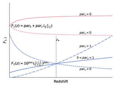
Figure 1: The variation of the parameter in SFE. The red ($F_{1}(z)$) and blue ($F_{2}(z)$) colors represent the models defined by Moster et al. (2018) and Sabti et al. (2022b), respectively. For example, $\epsilon_{\rm N}$ is described by $\epsilon_{0}+\epsilon_{z}(\frac{z}{z+1})$ following $F_{1}(z)$ or $10^{\epsilon_{i}}(\frac{1+z}{1+z_{*}})^{\epsilon_{s}}$ following $F_{2}(z)$. Other parameters $M_{1}$, $\gamma$ and $\beta$ have the same definitions. Therefore, these two different formulae need 2 or 3 free variables and present different variable spaces. $z_{*}$ presents the specific redshift value defined in Equation 12.

2.4 Bayesian analysis

With the comprehensive UV LF model in hand, we aim to investigate the evolution of SFE and cosmological parameters. To accommodate the asymmetric and unequal error bars, we employed an asymmetric Gaussian distribution (Kiziltan et al., 2013) as the likelihood function over the redshift range from 4 to 10, i.e.,

$${\rm Likelihood}=\prod^{N}_{i}{{\rm AN}}(f(x_{i})-y_{i}|c_{i},d_{i}),$$ (13)

where $(x_{i},y_{i})$ are the observational data points, $f(x_{i})$ represents the predicted values, $d_{i}$ serves as a scale parameter, and $c_{i}$ is the asymmetry parameter. The priors for all primary parameters are detailed in Table 1. For an optimal balance between accuracy and efficiency, we implemented the nested sampling method, utilizing Pymultinest for Bayesian parameter estimation. We configured the analysis with 1000 live points and an evidence tolerance of 0.5 to terminate the sampling process.

Table 1: Prior distributions of the parameters for SFE

Parameters	Priors of parameter inference
$\epsilon_{i}$	Uniform(-3, 3)
$\epsilon_{s}$	Uniform(-3, 3)
$M_{1,i}$	Uniform(7, 15)
$M_{1,s}$	Uniform(-7, 7)
$\beta_{i}$	Uniform(-3, 3)
$\beta_{s}$	Uniform(-3, 3)
$\gamma_{i}$	Uniform(-3, 3)
$\gamma_{s}$	Uniform(-3, 3)
$z_{*}$	Uniform(0, 10)
$\sigma_{8}$	0.812 or Uniform(0.1, 1.5)a

• ^a Note that, in the first scenario (discussing the evolution of SFE and reionization process), we use the former; otherwise, we use the latter.

3 Results

In this section, we present the fitting results under two scenarios. Initially, all parameters listed in Table 1 are evaluated within $\rm\Lambda$CDM framework (Planck Collaboration et al., 2020). This allows for an in-depth exploration of various reionization processes through the analysis of the derived UV luminosity density. Then, we assume $\sigma_{8}$ to be free and consider several additional datasets to evaluate the capability of constraining cosmological parameters by UV LFs.

3.1 The Evolution of SFE and UV LFs

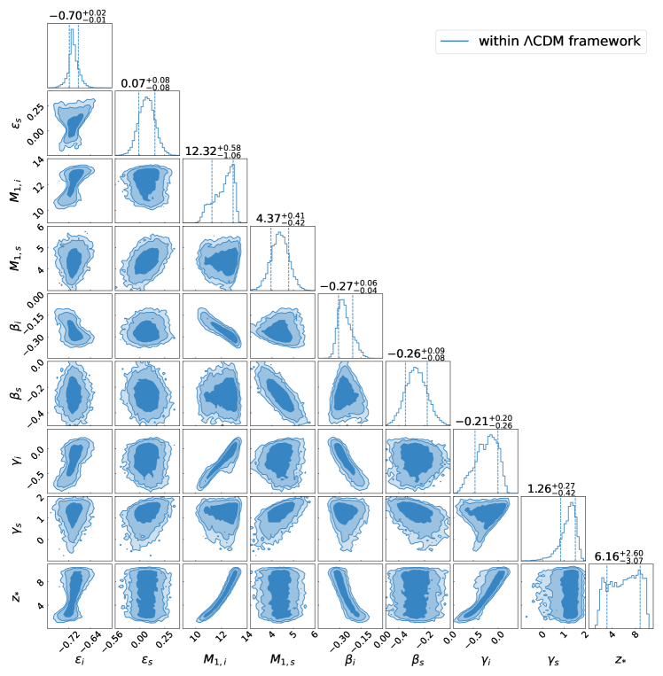
Figure 8: Posterior distributions of the SFE parameters for the UV LFs presented in Figure 2. The contours are at the 68%, 95%, and 99% credible level, respectively. The reported values are at the 68% credible level.

As shown in Figure 2, we present the best-fit UV LFs and SFE, alongside the observations. The corresponding posterior distributions are shown in Figure 8. For a better view, we present the UV LFs rather than the numbers of galaxies that are used practically. It is evident that the UV LF model fits well with the observations except for the data points at the bright end, which may be attributed to the contribution from active galactic nuclear (Harikane et al., 2022) in addition to the galaxy UV LFs. The corresponding distributions of the evolved SFE are consistent with other researches (such as Fig. 2 in Wechsler & Tinker (2018)). The SFE peaks at $M_{1}\sim 10^{11.67}M_{\odot}$ for $z=4$ and $10^{13.11}\,\rm M_{\odot}$ for $z=10$ (note that the latter is only obtained for extrapolation since the extremely bright end of the UV LFs has not been detected at $z\geq 8$). At low halo masses, the profile of SFE is determined by $\beta$, which remains almost constant with $\beta\sim 0.50$ across wide redshift range. Conversely, at high masses, $\gamma$ dominates the profile which varies from $\sim 0.44$ to $\sim 1.39$, resulting in a notable steepening of the SFE. However, at $z\geq 8$, due to the absence of UV LFs at the bright end, the SFE profile at $M_{1}\geq 10^{12}\,\rm M_{\odot}$ can not be well constrained. Consequently, it remains inconclusive whether there is a reliable evolution of the SFE at high masses.

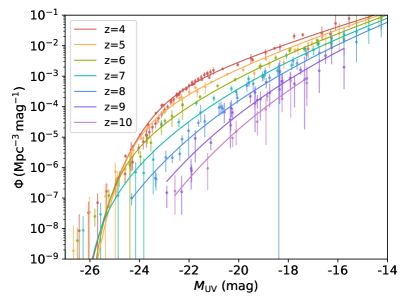
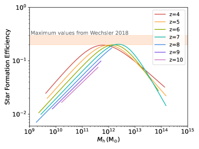
Figure 2: The left panel shows the observations of UV LFs and the best-fit results in the redshift range of $4\leq z\leq 10$. The right panel shows the corresponding distributions of SFE. The light orange region represents the range of maximum value (20%-30%) of SFE (Wechsler & Tinker, 2018). Due to the redshift-dependent nature of SFE, which connects all observations at each redshift, the estimated UV LFs are tightly constrained. Therefore, only the best-fit results are shown.

Based on the fitting results of SFE, the entire UV LFs in the redshift range of $4\leq z\leq 10$ can be described. By integrating over a proper range of the absolute magnitude, the UV luminosity densities $\rho$ can be calculated by

$$\rho_{\rm UV}=\int^{M_{\rm trunc}}_{-\infty}\Phi_{{\rm UV}}(M)M_{{\rm UV}}(M){\rm d}M,$$ (14)

where $M_{\rm trunc}$ denotes the truncation magnitude of the UV LFs. In general, $M_{\rm trunc}=-17$ corresponds to the SFR of $0.3\,\rm M_{\odot}\,yr^{-1}$ (Finkelstein et al., 2015; Bouwens et al., 2020; Oesch et al., 2018; Harikane et al., 2022). Additionally, we consider another truncated limit with $M_{\rm trunc}=-15$ following McLeod et al. (2016) and Ishigaki et al. (2018). As shown in Figure 3, the UV luminosity densities derived from the fitted UV LFs are in accordance with other observations. The empirical equation Eq.(15) in Madau & Dickinson (2014) fits well with the observations at low redshifts (i.e., $z\leq 6.5$) but tends to overestimate the UV luminosity density and the SFR density at higher redshifts.

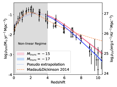
Figure 3: The evolution of the derived cosmic SFR density and UV luminosity density. The blue and red solid lines depict the best-fit values of UV LFs with $M_{\rm trunc}=-17$ and $M_{\rm trunc}=-15$, respectively. The blue and red dotted lines are the pseudo extrapolation to low redshift range. The light blue and red shades indicate the 90% credible regions. The orange dashed line denotes the analytical form derived by Madau & Dickinson (2014). The grey region $0\leq z\leq 4$ implicates that the galaxy evolution is in a highly non-linear stage, which can not be analyzed using the UV LF model. The black error bars are not considered in Bayesian analysis and are solely included for comparison with our predictions. These observations encompass the radio, near-infrared, H$\alpha$ and UV bands at the redshift range of $4\leq z\leq 10.5$ (Madau & Dickinson, 2014; Bouwens et al., 2015; Finkelstein et al., 2015; McLeod et al., 2016; Moster et al., 2018; Bouwens et al., 2020; Harikane et al., 2023).

3.2 Properties of the Reionization

Table 2: The observations of $x_{\rm H_{I}}$

redshift	$x_{\rm H_{I}}$	Publication
5.913	$0.3_{-0.2}^{+0.2}$	Totani et al. (2014)
6.2	$0.025_{-0.015}^{+0.015}$	Fan et al. (2006)
6.6	$0.15_{-0.15}^{+0.15}$	Ouchi et al. (2018)
6.6	$0.3_{-0.2}^{+0.2}$	Konno et al. (2018)
6.6	$0.08_{-0.05}^{+0.08}$	Morales et al. (2021)
7.0	$0.48_{-0.16}^{+0.16}$	Ota et al. (2008)
7.0	$0.59_{-0.15}^{+0.11}$	Mason et al. (2018)
7.0	$0.7_{-0.23}^{+0.20}$	Wang et al. (2020)
7.0	$0.55_{-0.13}^{+0.11}$	Whitler et al. (2020)
7.0	$0.28_{-0.05}^{+0.05}$	Morales et al. (2021)
7.09	$0.48_{-0.26}^{+0.26}$	Davies et al. (2018)
7.12	$0.54_{-0.54}^{+0.13}$	Umeda et al. (2023)
7.3	$0.55_{-0.25}^{+0.25}$	Konno et al. (2014)
7.3	$0.5_{-0.3}^{+0.1}$	Inoue et al. (2018)
7.3	$0.83_{-0.07}^{+0.06}$	Morales et al. (2021)
7.44	$0.69_{-0.38}^{+0.30}$	Umeda et al. (2023)
7.5	$0.88_{-0.10}^{+0.05}$	Hoag et al. (2019)
7.5	$0.21_{-0.19}^{+0.17}$	Greig et al. (2019)
7.54	$0.60_{-0.23}^{+0.20}$	Davies et al. (2018)
7.6	$0.88_{-0.10}^{+0.05}$	Hoag et al. (2019)
7.6	$0.49_{-0.19}^{+0.19}$	Jung et al. (2020)
8.28	$0.92_{-0.56}^{+0.08}$	Umeda et al. (2023)
10.28	$0.94_{-0.41}^{+0.06}$	Umeda et al. (2023)
11.48	$0.85_{-0.3}^{+0.15}$	Curtis-Lake et al. (2023)
5.6	$<0.09$	McGreer et al. (2015)
5.9	$<0.06$	McGreer et al. (2015)
6.3	$<0.17$	Totani et al. (2006)
6.6	$<0.5$	Sobacchi & Mesinger (2014)
7	$<0.6$	Whitler et al. (2020)
7.3	$>0.28$	Goto et al. (2021)
7.88	$>0.45$	Morishita et al. (2023)
8	$>0.76$	Mason et al. (2019)
10.17	$>0.9$	Hsiao et al. (2023)
10.6	$<0.88$	Bruton et al. (2023)
6-7	$x_{\rm H_{I}}(7)-x_{\rm H_{I}}(6)\geq 0.4$	Greig & Mesinger (2017)

Since the UV luminosity density covers the range of $4\leq z\leq 10$, it can be used to analyze the process of reionization. Robertson et al. (2013) described the evolution of the ionized hydrogen fraction $\mathcal{Q}_{\rm H_{II}}$ as

$$\dot{\mathcal{Q}}_{\rm H_{II}} =\frac{\dot{n}_{\rm ion}}{\langle n_{\rm H}\rangle}-\frac{\mathcal{Q}_{\rm H_{II}}}{t_{\rm tec}},$$ (15)

$$\dot{n}_{\rm ion} \equiv\langle f_{\rm esc}\xi_{\rm ion}\rangle\rho_{\rm UV},$$

$$\langle n_{\rm H}\rangle =\frac{X_{\rm p}{\rm\Omega_{\rm b}\rho_{\rm c}}}{m_{\rm H}},$$

$$t_{{\rm rec}} =\frac{1}{C_{{\rm H_{II}}}\alpha_{{\rm B}}(T)(1+Y_{{\rm p}}/4X_{{\rm p}})\langle n_{{\rm H}}\rangle(1+z)^{3}},$$

where $\langle n_{\rm H}\rangle$ is the mean hydrogen number density, $\dot{n}_{\rm ion}$ is the production rate of ionizing photons, and $t_{\rm tec}$ is the average recombination time in the IGM. Other parameters are defined as follows: the primordial mass fraction of hydrogen $X_{\rm p}=0.75$, the primordial helium abundance $Y_{\rm p}=1-X_{\rm p}$, the critical mass density $\rho_{c}=8.535\times 10^{-30}\,\rm g\,cm^{-3}$, the mass of hydrogen atom $m_{\rm H}=1.66\times 10^{-24}\,\rm g$, the coefficient for case B recombination $\alpha_{{\rm B}}=2.6\times 10^{-13}\,{\rm cm^{3}\,s^{-1}}$ (Sun & Furlanetto, 2016), and the clumping factor $C_{\rm H_{II}}=2.9\times\big{[}\frac{(1+z)}{6}\big{]}^{-1.1}$. The integral product of the ionizing photon production efficiency $\xi_{\rm ion}$ and the escape fraction $f_{\rm esc}$ are regarded as variables during model fitting. The evolution of $\mathcal{Q}_{\rm H_{II}}$ can be depicted after considering two extra boundary conditions,

$$\mathcal{Q}_{\rm H_{II}}(z_{0})=1\quad{\rm and}\quad\mathcal{Q}_{\rm H_{II}}(z_{\rm max})=0,$$ (16)

where $z_{0}$ and $z_{\rm max}$ are the redshift at the beginning and the end of the reionization, respectively.

Table 3: Prior distributions and posterior results of the parameters for $\mathcal{Q}_{\rm H_{II}}$

Parameters	Priors	Posterior resultsa
$z_{0}$	Uniform(0,10)	$5.38^{+0.65}_{-0.70}\,(5.52^{+0.60}_{-0.79})$
$z_{\rm max}$	Uniform(10,30)	$20.58^{+6.25}_{-6.75}\,(20.33^{+6.20}_{-6.69})$
$f_{\rm esc}$b	Uniform(0,1)	$0.43^{+0.02}_{-0.02}\,(0.28^{+0.01}_{-0.02})$

• ^a The values in these rows represent $\rho_{\rm UV}$ follows $M_{\rm trunc}=-15$. The uncertainties correspond to the $68\%$ confidence level.

• ^b During fitting process, $\xi_{\rm ion}$ is assumed to be $10^{24.5}$ for convenient analysis, but $\langle f_{\rm esc}\xi_{\rm ion}\rangle$ is still the practical fitting parameters.

Whereafter, the evolution of $\mathcal{Q}_{\rm H_{II}}$ can be constrained by the observations of the neutral hydrogen fraction $x_{\rm H_{I}}$ ($x_{\rm H_{I}}=1-\mathcal{Q}_{\rm H_{II}}$). These additional data were obtained through various methods, including analysis of the ${\rm Ly}\alpha$ and ${\rm Ly}\beta$ forests of quasars, distributions of ${\rm Ly}\alpha$ equivalent width, adsorptions in ${\rm Ly}\alpha$ damping wings, fractions of ${\rm Ly}\alpha$ emitters, the afterglow spectrum of the gamma-ray burst, and the Gunn Peterson troughs. All of the observation results are summarized in Table 2.

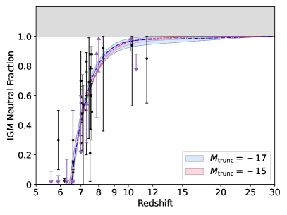
Figure 4: The evolution of the IGM neutral fraction. The black error bars and the purple bounds are the fitting data that listed in Table 2. The red and blue lines correspond to the results shown in Figure 3. The light-colored regions indicate the $90\%$ confidence level.

Besides, the Thomson optical depth to microwave background can be obtained by integrating $\mathcal{Q}_{\rm H_{II}}$,

$$\tau_{e}(z)=\int^{z}_{0}\frac{c(1+z^{\prime})^{2}}{H(z^{\prime})}\mathcal{Q}_{{\rm H_{II}}}\sigma_{{\rm T}}\langle n_{{\rm H}}\rangle\bigg{(}1+\eta\frac{Y_{{\rm p}}}{4X_{{\rm p}}}\bigg{)}{\rm d}z^{\prime},$$ (17)

where $\sigma_{\rm T}$ is the Thomson cross-section ($\sigma_{\rm T}=6.65\times 10^{-29}\,{\rm m^{2}}$), $\eta=1$ at $z>4$ and $\eta=2$ at $z\leq 4$. Thus, the observation of $\tau_{\rm e}$ ($\tau_{\rm e}=0.054\pm 0.007$) can be used to constrain $\mathcal{Q}_{\rm H_{II}}$. The Bayesian analysis follows the same process described in subsection 2.4. For these upper and lower limits, the likelihood functions are assumed to be uniform within the limited range and to be a half-Gaussian beyond the boundary (Greig & Mesinger, 2017). The prior distributions and the posterior results of the free parameters are listed in Table 3. Using the $\rho_{\rm UV}$ derived from UV LFs (at $z>10$, the $\rho_{\rm UV}$ is extrapolated), the estimated evolution of $x_{\rm H_{I}}$ is shown in Figure 4. Furthermore, we find out that the reionization started at $20.58^{+6.25}_{-6.75}\,(20.33^{+6.20}_{-6.69})$ and ended at $5.38^{+0.65}_{-0.70}\,(5.52^{+0.60}_{-0.79})$ when $M_{\rm trunc}$ is fixed to $-17\,(-15)$. Interestingly, such results are insensitive on the choice of $M_{\rm trunc}$.

Since Equation 17 describes the relation between $\mathcal{Q}_{\rm H_{II}}$ and $\tau_{\rm e}$, we evaluate $\tau$ by fitting observations of $x_{\rm H_{I}}$ listed in Table 2. Using $\rho_{\rm UV}$ with $M_{\rm trunc}=-17$, we present the extrapolated projections of $\tau_{\rm e}$ in Figure 5. Notably, our estimation is consistent with the result of Planck Collaboration et al. (2020), demonstrating the validity and reliability of our model.

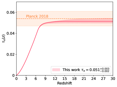
Figure 5: The predicted distribution of $\tau_{\rm e}$. The shaded pink region represents $68\%$ credible uncertainty range for $\tau_{\rm e}$. The light orange shade corresponds to the estimation provided by Planck Collaboration et al. (2020).

3.3 The constraints of the cosmological parameters

As discussed in section 2, the luminosity of galaxies relies on a specific cosmological framework, particularly $H_{0}$, $\Omega_{\rm m}$ and $\sigma_{8}$. However, these parameters degenerate with the parameters of SFE apparently, since SFE dictate SFR, $\sigma_{8}$ governs the relative density of DM halos, and $\Omega_{\rm m}$ and $H_{0}$ influence the density of galaxies through regulating $H(z)$. Therefore, additional constraints or supplementary dataset are required to narrow down the posterior parameter spaces within physical boundaries, especially for $H_{0}$ and $\Omega_{\rm m}$ because of their insensitivity to UV LFs. In light of this, we refer to the previous works of both Moster et al. (2018) and Sabti et al. (2022b), considering three comparative cases:

$Case\,1:$ To estimate $\sigma_{8}$, $\beta$ and $\gamma$ are assumed to be redshift-independence (i.e., $\beta_{s}=0$ and $\gamma_{s}=0$).

$Case\,2:$ To estimate $\sigma_{8}$, $\gamma$ is assumed to be redshift-independence (i.e., $\gamma_{s}=0$).

$Case\,3:$ To estimate $\sigma_{8}$, $\Omega_{\rm m}$ and $H_{0}$. Pantheon+ dataset (Scolnic et al., 2022) and a prior constraint on $\Omega_{\rm b}$ (Pisanti et al., 2021) are incorporated, and $\gamma$ is assumed to be redshift-independence (i.e., $\gamma_{s}=0$). The prior of the absolute B-band magnitude for the fiducial SN Ia is constrained within $[-20,-18]$ and the prior of $\Omega_{\rm b}$ follows the Gaussian distribution with $\mu=0.2233$ and $\sigma=0.00036$. The priors of $H_{0}$ and $\rm\Omega_{m}$ follow a Uniform distribution within $[50,90]$ and $[0.05,0.99]$, respectively.

Additionally, the maximum values of SFE are limited in $[0.01,0.5]$, which well covers the typical value $\sim 0.2-0.3$ found in previous analysis (Wechsler & Tinker, 2018). Furthermore, the parameter $M_{1,s}$ is bounded within $[-3,3]$, following the constraints from Sabti et al. (2022b).

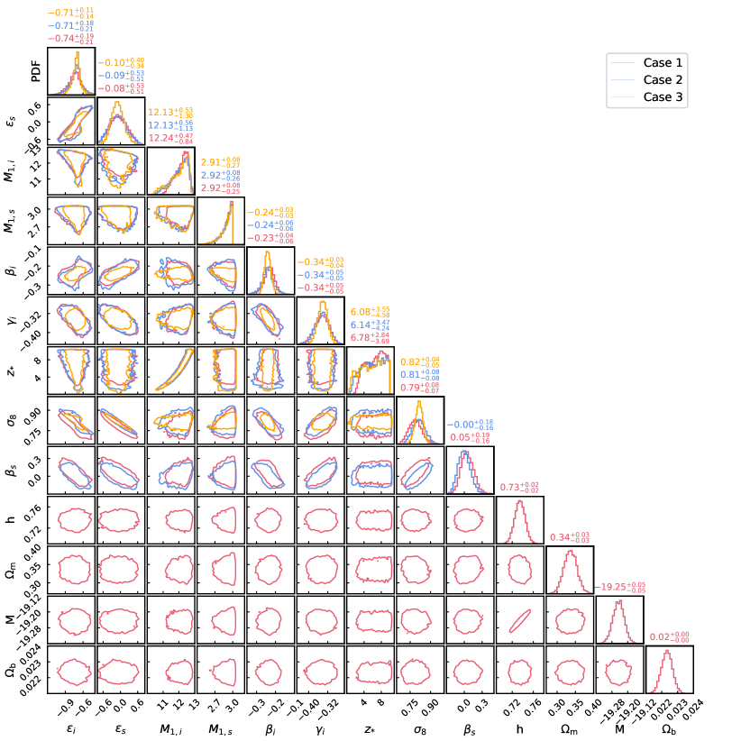
Figure 9: Complete posterior distributions of the SFE parameters and cosmological parameters for case 1, case 2 and case 3. All of the ranges are at the $90\%$ credible level.

The posterior distributions of estimated $\sigma_{8}$ are shown in Figure 6, which are more consistent with that obtained from early universe measurement. In $case\,3$, the contours of $H_{0}$, $\Omega_{\rm m}$, and $\sigma_{8}$ are depicted in Figure 7, resembling the results of Sabti et al. (2022b). Because we utilize a larger amount of data and align the observations within the same framework, our result of $\sigma_{8}=0.787^{+0.048}_{-0.047}$ reduces the uncertainty by $\sim 60\%$ compared to the estimation (i.e., $\sigma_{8}=0.76^{+0.12}_{-0.14}$) from Sabti et al. (2022b). The complete posterior results of these three cases are shown in Figure 9. It is worth noting that all estimated parameters are well converged except for $M_{1,s}$, which tends to converge towards a higher value close to the upper limit as Sabti et al. (2022b) derived. Furthermore, due to the insensitivity to UV LF, the constraints on $H_{0}$ and $\Omega_{\rm m}$ are not significantly improved in comparison to that derived by sole Pantheon+ dataset.

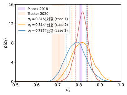
Figure 6: The results of $\sigma_{8}$ in three cases. To present the $\sigma_{8}$ tension, the purple and light orange regions represent the estimated $\sigma_{8}$ from Planck Collaboration et al. (2020) and Tröster et al. (2020), respectively.

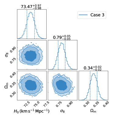
Figure 7: The posterior results of $H_{0}$, $\sigma_{8}$, and $\Omega_{\rm m}$ for $case\,3$. The contours indicate the $68\%$, $95\%$, $99\%$ credible levels. The values are at $68\%$ credible level.

4 Conclusions and discussions

Over the passed several years, numerous/various galaxy surveys accumulated a wealth of observations. Especially, the observed UV LFs span a wide range of redshift, from the local universe to very high-redshift ($z\sim 16$), providing the opportunity to study the epochs of cosmic dawn, reionization, and cosmic noon. In this work, we have developed a general UV LF model incorporating a redshift-dependent SFE and an alterable cosmological framework to explore the evolution of SFE, the process of reionization, and several cosmological parameters. By “correcting“ the observations to eliminate the effect of dust attenuation and reconcile the discrepancies of different cosmological frameworks, our results have higher precision compared with other works.

Under the framework of $\Lambda$CDM, the UV LFs within the redshift range of $z=4-10$ can constrain the evolution of SFE stringently. In Figure 2, the profile of SFE shows a clear tendency of evolution with redshift, particularly in the low mass range. The corresponding mass of the DM halos ($\sim 10^{12}\,\rm M_{\odot}$) at maximum SFE ($\sim 20\%$) presents a shift towards higher values, although further investigation is needed/warranted. Since the variable feedback mechanism and the environmental factors influence the relative strength of SFE, disentangling the contributions of each component solely from UV LFs poses challenges. Fortunately, dynamical simulations provide comparisons for these elements(e.g., Guszejnov et al., 2022; Scharré et al., 2024), including the IMF, stellar radiation, stellar winds, supernovae, AGN and others. Therefore, once the profile of SFE can be constrained by other methods beyond UV LFs, the cosmological researches relying on UV LFs can yield more precise results, as the intrinsic degeneracy between SFE and cosmological parameters is alleviated. Furthermore, based on the derived UV luminosity density and abundant observations of the IGM neutral fraction, the beginning and ending redshifts of the reionization epoch are constrained to $20.58^{+6.25}_{-6.75}$ ($20.33^{+6.20}_{-6.69}$) and $5.38^{+0.65}_{-0.70}$ ($5.52^{+0.60}_{-0.79}$) with $M_{\rm trunc}=-17$ and $-15$, respectively. If considering the observations of UV LFs at $z>10$, $\rho_{\rm UV}$ will be much higher than the extrapolated ones (Donnan et al., 2023; Harikane et al., 2023), but does not impact Figure 4 notably. We validate the reliability of our model by comparing the inferred Thomson scattering optical depth $\tau_{\rm e}$ with the result of Planck Collaboration et al. (2020). Nonetheless, our model is applicable only to the nonlinear regime and not to regimes with $z>10$, as uncertainties in stellar populations and dust attenuation lead to large uncertainties of SFE (Inayoshi et al., 2022; Wang et al., 2023) and other parameters.

On the other hand, we attempt to analyze cosmology by UV LF observations. Similar to previous works, we find that only introducing some reasonable and additional information, the cosmological parameters can be constrained within physically meaningful scopes. Within a specific parameter space, we obtain $\sigma_{8}=0.815^{+0.026}_{-0.030}$, which is consistent with the $\Lambda$CDM framework. Moreover, following Sabti et al. (2022b) and employing the same dataset and parameter spaces, the inferred $\sigma_{8}=0.784^{+0.051}_{-0.048}$ has a better precision, improved by $\sim 2-3$ times compared to the results reported by Sabti et al. (2022b). It is in line with expectations since $\sigma_{8}$ is constrained by UV LFs mainly and the number of UV LF observations we used is over four times greater than they used, thereby reducing the error to $\sim 0.12/\sqrt{4}$. Besides the increase of data points, the expansion of galaxy survey areas decrease the uncertainties of cosmic variance and then improve the accuracy of cosmology analysis.

In the foreseeable future, various galaxy survey projects will make remarkable progresses. The Large Synoptic Survey Telescope (Ivezić et al., 2019), the Roman Space Telescope (Eifler et al., 2021), Euclid (Laureijs et al., 2011), the Extremely Large Telescope (Gilmozzi & Spyromilio, 2007), and the China Space Station Telescope (Zhan, 2011) will explore the Universe in deep field, providing extensive observational data with sufficient precision and covering a wide range of redshift. Furthermore, with the improving accuracy of dynamical simulation, the profile of SFE will be understood in depth, thereby breaking the intrinsic degeneracy between the SFE parameters and cosmological parameters. Consequently, through future observations of UV LFs and additional simulated constraints, there will be opportunities to analyze cosmological model, galaxy evolution, and the epoch of reionization with greater precision and to a more complete understanding in the future.

5 Acknowledgements

This work is supported in part by NSFC under grants of No. 11921003, No. 12233011 and 12303056; S.-P. T. acknowledges support from the General Fund (No. 2023M733736) of the China Postdoctoral Science Foundation; G.-W. Y. acknowledges support from the University of Trento and the Provincia Autonoma di Trento (PAT, Autonomous Province of Trento) through the UniTrento Internal Call for Research 2023 grant “Searching for Dark Energy off the beaten track” (DARKTRACK, grant agreement no.E63C22000500003, PI: Sunny Vagnozzi).

Software: Pymultinest (Buchner (2016), version 2.11, https://pypi.org/project/pymultinest/), HMFcalc (Murray (2014)), https://github.com/halomod/hmf/

Appendix A The posterior distributions of the parameters of SFE model

Here, we present the whole posterior distributions of SFE parameters mentioned in subsection 3.1 and the detailed results for Case 1, Case 2, and Case 3 in subsection 3.3.

References

- Adams et al. (2023a) Adams, N. J., Bowler, R. A. A., Jarvis, M. J., Varadaraj, R. G., & Häußler, B. 2023a, MNRAS, 523, 327, doi: 10.1093/mnras/stad1333
- Adams et al. (2023b) Adams, N. J., Conselice, C. J., Austin, D., et al. 2023b, arXiv e-prints, arXiv:2304.13721, doi: 10.48550/arXiv.2304.13721
- Ashton et al. (2022) Ashton, G., Bernstein, N., Buchner, J., et al. 2022, Nature Reviews Methods Primers, 2, 39, doi: 10.1038/s43586-022-00121-x
- Atek et al. (2024) Atek, H., Labbé, I., Furtak, L. J., et al. 2024, Nature, 626, 975, doi: 10.1038/s41586-024-07043-6
- Bell et al. (2003) Bell, E. F., McIntosh, D. H., Katz, N., & Weinberg, M. D. 2003, ApJ, 585, L117, doi: 10.1086/374389
- Berlind et al. (2003) Berlind, A. A., Weinberg, D. H., Benson, A. J., et al. 2003, ApJ, 593, 1, doi: 10.1086/376517
- Bond et al. (1991) Bond, J. R., Cole, S., Efstathiou, G., & Kaiser, N. 1991, ApJ, 379, 440, doi: 10.1086/170520
- Bouwens et al. (2020) Bouwens, R., González-López, J., Aravena, M., et al. 2020, ApJ, 902, 112, doi: 10.3847/1538-4357/abb830
- Bouwens et al. (2022) Bouwens, R. J., Illingworth, G., Ellis, R. S., Oesch, P., & Stefanon, M. 2022, ApJ, 940, 55, doi: 10.3847/1538-4357/ac86d1
- Bouwens et al. (2012) Bouwens, R. J., Illingworth, G. D., Oesch, P. A., et al. 2012, ApJ, 754, 83, doi: 10.1088/0004-637X/754/2/83
- Bouwens et al. (2014) —. 2014, ApJ, 793, 115, doi: 10.1088/0004-637X/793/2/115
- Bouwens et al. (2015) —. 2015, ApJ, 803, 34, doi: 10.1088/0004-637X/803/1/34
- Bouwens et al. (2021) Bouwens, R. J., Oesch, P. A., Stefanon, M., et al. 2021, AJ, 162, 47, doi: 10.3847/1538-3881/abf83e
- Bouwens et al. (2023) Bouwens, R. J., Stefanon, M., Brammer, G., et al. 2023, MNRAS, 523, 1036, doi: 10.1093/mnras/stad1145
- Bower (1991) Bower, R. G. 1991, MNRAS, 248, 332, doi: 10.1093/mnras/248.2.332
- Bowler et al. (2020) Bowler, R. A. A., Jarvis, M. J., Dunlop, J. S., et al. 2020, MNRAS, 493, 2059, doi: 10.1093/mnras/staa313
- Bruton et al. (2023) Bruton, S., Lin, Y.-H., Scarlata, C., & Hayes, M. J. 2023, ApJ, 949, L40, doi: 10.3847/2041-8213/acd5d0
- Buchner (2016) Buchner, J. 2016, PyMultiNest: Python interface for MultiNest, Astrophysics Source Code Library, record ascl:1606.005. http://ascl.net/1606.005
- Chevallard et al. (2015) Chevallard, J., Silk, J., Nishimichi, T., et al. 2015, MNRAS, 446, 3235, doi: 10.1093/mnras/stu2280
- Corasaniti et al. (2017) Corasaniti, P. S., Agarwal, S., Marsh, D. J. E., & Das, S. 2017, Phys. Rev. D, 95, 083512, doi: 10.1103/PhysRevD.95.083512
- Correa et al. (2015) Correa, C. A., Wyithe, J. S. B., Schaye, J., & Duffy, A. R. 2015, MNRAS, 450, 1514, doi: 10.1093/mnras/stv689
- Croton et al. (2006) Croton, D. J., Springel, V., White, S. D. M., et al. 2006, MNRAS, 365, 11, doi: 10.1111/j.1365-2966.2005.09675.x
- Curtis-Lake et al. (2023) Curtis-Lake, E., Carniani, S., Cameron, A., et al. 2023, Nature Astronomy, 7, 622, doi: 10.1038/s41550-023-01918-w
- Davies et al. (2018) Davies, F. B., Hennawi, J. F., Bañados, E., et al. 2018, ApJ, 864, 143, doi: 10.3847/1538-4357/aad7f8
- Dekel & Birnboim (2006) Dekel, A., & Birnboim, Y. 2006, MNRAS, 368, 2, doi: 10.1111/j.1365-2966.2006.10145.x
- Donnan et al. (2023) Donnan, C. T., McLeod, D. J., Dunlop, J. S., et al. 2023, MNRAS, 518, 6011, doi: 10.1093/mnras/stac3472
- Donnan et al. (2024) Donnan, C. T., McLure, R. J., Dunlop, J. S., et al. 2024, arXiv e-prints, arXiv:2403.03171, doi: 10.48550/arXiv.2403.03171
- Eifler et al. (2021) Eifler, T., Miyatake, H., Krause, E., et al. 2021, MNRAS, 507, 1746, doi: 10.1093/mnras/stab1762
- Fan et al. (2006) Fan, X., Strauss, M. A., Becker, R. H., et al. 2006, AJ, 132, 117, doi: 10.1086/504836
- Finkelstein et al. (2015) Finkelstein, S. L., Ryan, Russell E., J., Papovich, C., et al. 2015, ApJ, 810, 71, doi: 10.1088/0004-637X/810/1/71
- Finkelstein et al. (2019) Finkelstein, S. L., D’Aloisio, A., Paardekooper, J.-P., et al. 2019, ApJ, 879, 36, doi: 10.3847/1538-4357/ab1ea8
- Gilmozzi & Spyromilio (2007) Gilmozzi, R., & Spyromilio, J. 2007, The Messenger, 127, 11
- Goto et al. (2021) Goto, H., Shimasaku, K., Yamanaka, S., et al. 2021, ApJ, 923, 229, doi: 10.3847/1538-4357/ac308b
- Greig & Mesinger (2017) Greig, B., & Mesinger, A. 2017, MNRAS, 465, 4838, doi: 10.1093/mnras/stw3026
- Greig et al. (2019) Greig, B., Mesinger, A., & Bañados, E. 2019, MNRAS, 484, 5094, doi: 10.1093/mnras/stz230
- Guszejnov et al. (2022) Guszejnov, D., Grudić, M. Y., Offner, S. S. R., et al. 2022, MNRAS, 515, 4929, doi: 10.1093/mnras/stac2060
- Harikane et al. (2022) Harikane, Y., Ono, Y., Ouchi, M., et al. 2022, ApJS, 259, 20, doi: 10.3847/1538-4365/ac3dfc
- Harikane et al. (2023) Harikane, Y., Ouchi, M., Oguri, M., et al. 2023, ApJS, 265, 5, doi: 10.3847/1538-4365/acaaa9
- Hoag et al. (2019) Hoag, A., Bradač, M., Huang, K., et al. 2019, ApJ, 878, 12, doi: 10.3847/1538-4357/ab1de7
- Hopkins et al. (2012) Hopkins, P. F., Quataert, E., & Murray, N. 2012, MNRAS, 421, 3522, doi: 10.1111/j.1365-2966.2012.20593.x
- Hsiao et al. (2023) Hsiao, T. Y.-Y., Abdurro’uf, Coe, D., et al. 2023, arXiv e-prints, arXiv:2305.03042, doi: 10.48550/arXiv.2305.03042
- Inayoshi et al. (2022) Inayoshi, K., Harikane, Y., Inoue, A. K., Li, W., & Ho, L. C. 2022, ApJ, 938, L10, doi: 10.3847/2041-8213/ac9310
- Inoue et al. (2018) Inoue, A. K., Hasegawa, K., Ishiyama, T., et al. 2018, PASJ, 70, 55, doi: 10.1093/pasj/psy048
- Ishigaki et al. (2018) Ishigaki, M., Kawamata, R., Ouchi, M., et al. 2018, ApJ, 854, 73, doi: 10.3847/1538-4357/aaa544
- Ivezić et al. (2019) Ivezić, Ž., Kahn, S. M., Tyson, J. A., et al. 2019, ApJ, 873, 111, doi: 10.3847/1538-4357/ab042c
- Jiang et al. (2022) Jiang, L., Ning, Y., Fan, X., et al. 2022, Nature Astronomy, 6, 850, doi: 10.1038/s41550-022-01708-w
- Jung et al. (2020) Jung, I., Finkelstein, S. L., Dickinson, M., et al. 2020, ApJ, 904, 144, doi: 10.3847/1538-4357/abbd44
- Kiziltan et al. (2013) Kiziltan, B., Kottas, A., De Yoreo, M., & Thorsett, S. E. 2013, ApJ, 778, 66, doi: 10.1088/0004-637X/778/1/66
- Konno et al. (2014) Konno, A., Ouchi, M., Ono, Y., et al. 2014, ApJ, 797, 16, doi: 10.1088/0004-637X/797/1/16
- Konno et al. (2018) Konno, A., Ouchi, M., Shibuya, T., et al. 2018, PASJ, 70, S16, doi: 10.1093/pasj/psx131
- Krause & Eifler (2017) Krause, E., & Eifler, T. 2017, MNRAS, 470, 2100, doi: 10.1093/mnras/stx1261
- Lacey & Cole (1993) Lacey, C., & Cole, S. 1993, MNRAS, 262, 627, doi: 10.1093/mnras/262.3.627
- Laureijs et al. (2011) Laureijs, R., Amiaux, J., Arduini, S., et al. 2011, arXiv e-prints, arXiv:1110.3193, doi: 10.48550/arXiv.1110.3193
- Lewis et al. (2000) Lewis, A., Challinor, A., & Lasenby, A. 2000, ApJ, 538, 473, doi: 10.1086/309179
- Liu et al. (2024) Liu, Y., Gao, L., Bose, S., et al. 2024, MNRAS, 527, 11740, doi: 10.1093/mnras/stae003
- Madau & Dickinson (2014) Madau, P., & Dickinson, M. 2014, ARA&A, 52, 415, doi: 10.1146/annurev-astro-081811-125615
- Mason et al. (2015) Mason, C. A., Trenti, M., & Treu, T. 2015, ApJ, 813, 21, doi: 10.1088/0004-637X/813/1/21
- Mason et al. (2018) Mason, C. A., Treu, T., Dijkstra, M., et al. 2018, ApJ, 856, 2, doi: 10.3847/1538-4357/aab0a7
- Mason et al. (2019) Mason, C. A., Fontana, A., Treu, T., et al. 2019, MNRAS, 485, 3947, doi: 10.1093/mnras/stz632
- McGreer et al. (2015) McGreer, I. D., Mesinger, A., & D’Odorico, V. 2015, MNRAS, 447, 499, doi: 10.1093/mnras/stu2449
- McLeod et al. (2016) McLeod, D. J., McLure, R. J., & Dunlop, J. S. 2016, MNRAS, 459, 3812, doi: 10.1093/mnras/stw904
- McLure et al. (2013) McLure, R. J., Dunlop, J. S., Bowler, R. A. A., et al. 2013, MNRAS, 432, 2696, doi: 10.1093/mnras/stt627
- Meurer et al. (1999) Meurer, G. R., Heckman, T. M., & Calzetti, D. 1999, ApJ, 521, 64, doi: 10.1086/307523
- Morales et al. (2021) Morales, A. M., Mason, C. A., Bruton, S., et al. 2021, ApJ, 919, 120, doi: 10.3847/1538-4357/ac1104
- Morishita et al. (2023) Morishita, T., Roberts-Borsani, G., Treu, T., et al. 2023, ApJ, 947, L24, doi: 10.3847/2041-8213/acb99e
- Morishita & Stiavelli (2023) Morishita, T., & Stiavelli, M. 2023, ApJ, 946, L35, doi: 10.3847/2041-8213/acbf50
- Moster et al. (2018) Moster, B. P., Naab, T., & White, S. D. M. 2018, MNRAS, 477, 1822, doi: 10.1093/mnras/sty655
- Murray (2014) Murray, S. 2014, HMF: Halo Mass Function calculator, Astrophysics Source Code Library, record ascl:1412.006. http://ascl.net/1412.006
- Murray et al. (2013) Murray, S. G., Power, C., & Robotham, A. S. G. 2013, Astronomy and Computing, 3, 23, doi: 10.1016/j.ascom.2013.11.001
- Naidu et al. (2020) Naidu, R. P., Tacchella, S., Mason, C. A., et al. 2020, ApJ, 892, 109, doi: 10.3847/1538-4357/ab7cc9
- Oesch et al. (2018) Oesch, P. A., Bouwens, R. J., Illingworth, G. D., Labbé, I., & Stefanon, M. 2018, ApJ, 855, 105, doi: 10.3847/1538-4357/aab03f
- Oke & Gunn (1983) Oke, J. B., & Gunn, J. E. 1983, ApJ, 266, 713, doi: 10.1086/160817
- Ota et al. (2008) Ota, K., Iye, M., Kashikawa, N., et al. 2008, ApJ, 677, 12, doi: 10.1086/529006
- Ouchi et al. (2018) Ouchi, M., Harikane, Y., Shibuya, T., et al. 2018, PASJ, 70, S13, doi: 10.1093/pasj/psx074
- Overzier et al. (2011) Overzier, R. A., Heckman, T. M., Wang, J., et al. 2011, ApJ, 726, L7, doi: 10.1088/2041-8205/726/1/L7
- Padmanabhan & Loeb (2023) Padmanabhan, H., & Loeb, A. 2023, ApJ, 953, L4, doi: 10.3847/2041-8213/acea7a
- Pérez-González et al. (2023) Pérez-González, P. G., Costantin, L., Langeroodi, D., et al. 2023, ApJ, 951, L1, doi: 10.3847/2041-8213/acd9d0
- Pisanti et al. (2021) Pisanti, O., Mangano, G., Miele, G., & Mazzella, P. 2021, J. Cosmology Astropart. Phys, 2021, 020, doi: 10.1088/1475-7516/2021/04/020
- Planck Collaboration et al. (2020) Planck Collaboration, Aghanim, N., Akrami, Y., et al. 2020, A&A, 641, A6, doi: 10.1051/0004-6361/201833910
- Robertson et al. (2013) Robertson, B. E., Furlanetto, S. R., Schneider, E., et al. 2013, ApJ, 768, 71, doi: 10.1088/0004-637X/768/1/71
- Sabti et al. (2022a) Sabti, N., Muñoz, J. B., & Blas, D. 2022a, ApJ, 928, L20, doi: 10.3847/2041-8213/ac5e9c
- Sabti et al. (2022b) —. 2022b, Phys. Rev. D, 105, 043518, doi: 10.1103/PhysRevD.105.043518
- Salpeter (1955) Salpeter, E. E. 1955, ApJ, 121, 161, doi: 10.1086/145971
- Scharré et al. (2024) Scharré, L., Sorini, D., & Davé, R. 2024, arXiv e-prints, arXiv:2404.07252, doi: 10.48550/arXiv.2404.07252
- Scolnic et al. (2022) Scolnic, D., Brout, D., Carr, A., et al. 2022, ApJ, 938, 113, doi: 10.3847/1538-4357/ac8b7a
- Shen et al. (2023) Shen, X., Vogelsberger, M., Boylan-Kolchin, M., Tacchella, S., & Kannan, R. 2023, MNRAS, 525, 3254, doi: 10.1093/mnras/stad2508
- Sheth et al. (2001) Sheth, R. K., Mo, H. J., & Tormen, G. 2001, MNRAS, 323, 1, doi: 10.1046/j.1365-8711.2001.04006.x
- Sobacchi & Mesinger (2014) Sobacchi, E., & Mesinger, A. 2014, MNRAS, 440, 1662, doi: 10.1093/mnras/stu377
- Sun & Furlanetto (2016) Sun, G., & Furlanetto, S. R. 2016, MNRAS, 460, 417, doi: 10.1093/mnras/stw980
- Tacchella et al. (2013) Tacchella, S., Trenti, M., & Carollo, C. M. 2013, ApJ, 768, L37, doi: 10.1088/2041-8205/768/2/L37
- Totani et al. (2006) Totani, T., Kawai, N., Kosugi, G., et al. 2006, PASJ, 58, 485, doi: 10.1093/pasj/58.3.485
- Totani et al. (2014) Totani, T., Aoki, K., Hattori, T., et al. 2014, PASJ, 66, 63, doi: 10.1093/pasj/psu032
- Tröster et al. (2020) Tröster, T., Sánchez, A. G., Asgari, M., et al. 2020, A&A, 633, L10, doi: 10.1051/0004-6361/201936772
- Umeda et al. (2023) Umeda, H., Ouchi, M., Nakajima, K., et al. 2023, arXiv e-prints, arXiv:2306.00487, doi: 10.48550/arXiv.2306.00487
- Wang et al. (2020) Wang, F., Davies, F. B., Yang, J., et al. 2020, ApJ, 896, 23, doi: 10.3847/1538-4357/ab8c45
- Wang et al. (2023) Wang, Y.-Y., Lei, L., Yuan, G.-W., & Fan, Y.-Z. 2023, ApJ, 954, L48, doi: 10.3847/2041-8213/acf46c
- Wechsler & Tinker (2018) Wechsler, R. H., & Tinker, J. L. 2018, ARA&A, 56, 435, doi: 10.1146/annurev-astro-081817-051756
- Whitler et al. (2020) Whitler, L. R., Mason, C. A., Ren, K., et al. 2020, MNRAS, 495, 3602, doi: 10.1093/mnras/staa1178
- Willott et al. (2023) Willott, C. J., Desprez, G., Asada, Y., et al. 2023, arXiv e-prints, arXiv:2311.12234, doi: 10.48550/arXiv.2311.12234
- Winch et al. (2024) Winch, H., Rogers, K. K., Hložek, R., & Marsh, D. J. E. 2024, arXiv e-prints, arXiv:2404.11071, doi: 10.48550/arXiv.2404.11071
- Yang et al. (2003) Yang, X., Mo, H. J., & van den Bosch, F. C. 2003, MNRAS, 339, 1057, doi: 10.1046/j.1365-8711.2003.06254.x
- Yang et al. (2009) —. 2009, ApJ, 695, 900, doi: 10.1088/0004-637X/695/2/900
- Zhan (2011) Zhan, H. 2011, Scientia Sinica Physica, Mechanica & Astronomica, 41, 1441, doi: 10.1360/132011-961