Csikvári’s poset and Tutte polynomial

Abstract.

Csikvári constructed a poset on trees to prove that several graph functions attain extreme values at the star and the path among the trees on a fixed number of vertices. Reiner and Smith proved that the Tutte polynomials ${\mathbf{T}}(1,y)$ of cones over trees, which are the graphs obtained by attaching a cone vertex to a tree, have the described extreme behavior. They further conjectured that the result can be strengthened in terms of Csikvári’s poset. We solve this conjecture affirmatively.

1. Introduction

This paper aims to prove a conjecture of Victor Reiner and Dorian Smith. We first introduce some background.

Fix a positive integer $n\geq 3$ and consider the set ${\mathcal{T}}_{n}$ of all trees on $n$ vertices. In ${\mathcal{T}}_{n}$, two extreme elements are the tree $\text{Path}_{n}$ with exactly $2$ leaves and the tree $\text{Star}_{n}$ with exactly $n-1$ leaves. Many graph functions $F(G)$ attain extreme values at $\text{Star}_{n}$ and $\text{Path}_{n}$ among trees in ${\mathcal{T}}_{n}$. For example, Lovász and Pelikán [7] proved that the star has the largest spectral radius and the path has the smallest spectral radius among all trees in ${\mathcal{T}}_{n}$ (in short, we say that the function $F(G)$ can be the spectral radius of $G$); Zhou and Gutman [11] proved that $F(G)$ can be the coefficients of the characteristic polynomial of the Laplacian matrix of $G$; Péter Csikvári [4] proved that $F(G)$ can the number of closed walks of a fixed length $l$ in $G$. For more examples, see [5].

Among these works, Csikvári’s is of most interest to us. Csikvári’s main tool is an operation on ${\mathcal{T}}_{n}$ called the generalized tree shift, which makes ${\mathcal{T}}_{n}$ a partially ordered set. We call it the Csikvári poset. One basic feature of the Csikvári poset is that the tree $\text{Star}_{n}$ is the unique maximal element and the tree $\text{Path}_{n}$ is the unique minimal element [4, Corollary 2.5].

For the definition of Csikvári poset, see Section 2. For readers’ convenience, we quote the example of ${\mathcal{T}}_{7}$ from [10] here; see Figure 1. For the example of ${\mathcal{T}}_{6}$ , see [5, Figure 2].

The generalized tree shift indeed generalizes many transformations for trees found in the literature; see [5, Section 10] for a detailed discussion. Csikvári’s tree shift was inspired by a graph transformation defined by Kelmans in [6]. In [3], the tree shift is called the KC-transformation in honor of Kelmans and Csikvári. Csikvári’s tree shift was used to prove that several graph functions $F(G)$ have the property described in the first paragraph; see [4, 3, 5].

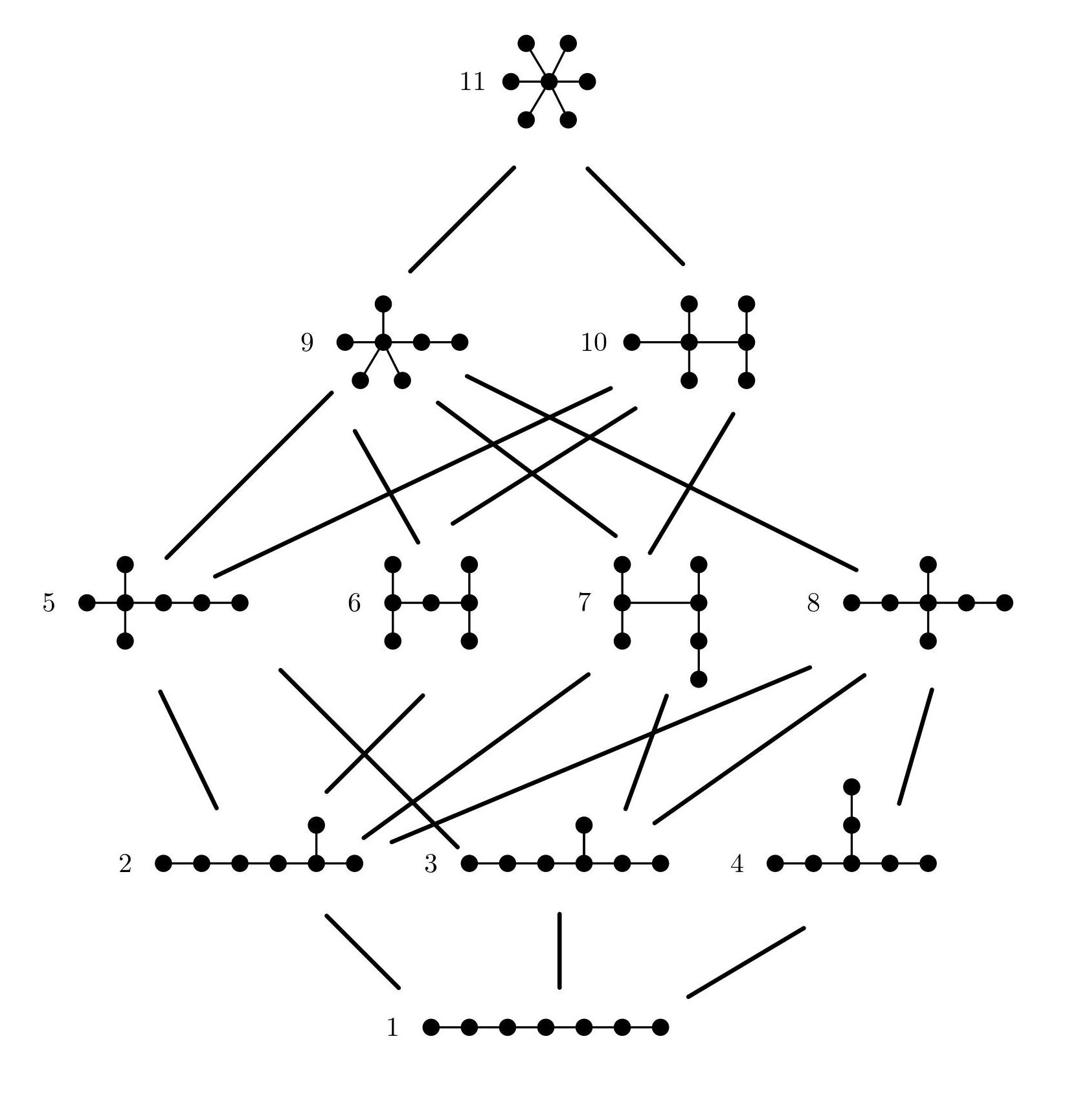
Figure 1. The Hasse diagram of the Csikvári poset on trees with $7$ vertices [10].

In [10], Victor Reiner and Dorian Smith studied the sandpile groups of graphs ${\text{Cone}(T)}$ obtained by attaching a cone vertex to a tree $T$. In particular, they studied the function

$$f(T):={\mathbf{T}}_{\text{Cone}(T)}(1,y),$$

where ${\mathbf{T}}_{G}(x,y)\in{\mathbb{Z}}[x,y]$ denotes the Tutte polynomial of a graph $G$.

In general, the coefficients of the Tutte polynomial ${\mathbf{T}}_{G}(1,y)$ encode some information from $G$ including external activities, the number of recurrent sandpile configurations (also known as critical configurations) at a given level, and the number of reduced divisors (also known as $G$-parking functions or superstable configurations) at a given level; see [8, 2, 1]. Via duality, ${\mathbf{T}}_{G}(1,y)$ can be viewed as the $h$-vector of the cographic matroid $M^{*}(G)$ [9].

Going back to Reiner and Smith’s work, they proved the following result.

Theorem 1.1.

[10, Theorem 1.4] For a tree $T\in{\mathcal{T}}_{n}$, the inequalities

$$f(\text{Star}_{n})\leq f(T)\leq f(\text{Path}_{n})$$

hold coefficientwise.

For readers’ convenience, we quote the values $f(T)$ for all the trees $T\in{\mathcal{T}}_{7}$ from [10]; see Table 1.

$T$	$f(T)$
1	$y^{6}+7y^{5}+26y^{4}+63y^{3}+104y^{2}+122y+64$
2	$y^{6}+7y^{5}+25y^{4}+59y^{3}+96y^{2}+104y+64$
3	$y^{6}+7y^{5}+25y^{4}+58y^{3}+94y^{2}+104y+64$
4	$y^{6}+7y^{5}+25y^{4}+57y^{3}+92y^{2}+104y+64$
5	$y^{6}+7y^{5}+24y^{4}+53y^{3}+83y^{2}+92y+64$
6	$y^{6}+7y^{5}+24y^{4}+55y^{3}+89y^{2}+96y+64$
7	$y^{6}+7y^{5}+24y^{4}+54y^{3}+86y^{2}+96y+64$
8	$y^{6}+7y^{5}+24y^{4}+52y^{3}+80y^{2}+92y+64$
9	$y^{6}+7y^{5}+23y^{4}+47y^{3}+68y^{2}+78y+64$
10	$y^{6}+7y^{5}+23y^{4}+49y^{3}+76y^{2}+84y+64$
11	$y^{6}+7y^{5}+22y^{4}+42y^{3}+57y^{2}+63y+64$

Table 1. The values $f(T)$ for all the trees $T\in{\mathcal{T}}_{7}$. See Figure 1 for the labels of the trees.

Victor Reiner and Dorian Smith conjectured and we will prove the following.

Conjecture 1.2.

[10, Conjecture 7.1] Let $T$ and $T^{\prime}$ be two trees. If $T<T^{\prime}$ in the Csikvári poset, then $f(T^{\prime})\leq f(T)$ coefficientwise in ${\mathbb{Z}}[y]$.

Note that the conjecture implies Theorem 1.1. Since our proof does not rely on Theorem 1.1 (or its proof), we obtain a new proof of Theorem 1.1. Comparing the proof in [10] and ours, one can notice that they deal with many inequalities while we mostly deal with equalities.

Remarkably, our proof makes use of what Csikvári called “General Lemma” ([5, Theorem 5.1]). In particular, when $T^{\prime}$ covers $T$ in the Csikvári poset, we can factor $f(T)-f(T^{\prime})$ into three polynomials with no negative coefficients (Proposition 3.2). Thus our result can be viewed as another successful application of Csikvári’s method in [5].

Our paper is arranged as follows. In Section 2, we give the necessary definitions and notations. In Section 3, we present the proof of Conjecture 1.2.

2. Preliminaries

2.1. Tutte polynomial and Cone of Tree

By a graph, we mean a finite undirected graph possibly with parallel edges and loops. Recall that the Tutte polynomial ${\mathbf{T}}_{G}(x,y)$ of a graph $G$ can be defined recursively by the following contraction-deletion relation.

$${\mathbf{T}}_{G}(x,y)=\begin{cases}{\mathbf{T}}_{G\setminus e}(x,y)+{\mathbf{T}}_{G/e}(x,y),&\text{if }e\text{ is neither a loop nor a bridge},\\ y\cdot{\mathbf{T}}_{G\setminus e}(x,y),&\text{if e is a loop,}\\ x\cdot{\mathbf{T}}_{G/e}(x,y),&\text{if e is a bridge,}\\ 1,&\text{if }G\text{ has no edges,}\end{cases}$$

where $G\setminus e$ (resp. $G/e$) is the graph obtained from $G$ by deleting (resp. contracting) the edge $e$. It follows that the coefficients of Tutte polynomials are non-negative integers.

By the contraction-deletion relation, it is easy to see that the trees in ${\mathcal{T}}_{n}$ cannot be distinguished by their Tutte polynomials. Following [10], we may consider the Tutte polynomials of the cones over trees to help with this issue.

Definition 2.1.

Let $G$ be a graph.

1. The cone over the graph $G$ is the graph obtained from $G$ by adding an extra vertex $r$ and then connecting $r$ to each vertex of $G$, denoted by $\text{Cone}(G)$.

2. Define the function

   $$f(G):={\mathbf{T}}_{\text{Cone}(G)}(1,y)\in{\mathbb{Z}}[y].$$

Definition 2.2.

Throughout our paper, for two polynomials $f_{1},f_{2}\in{\mathbb{Z}}[y]$, the inequality $f_{1}\leq f_{2}$ means that the coefficients of $f_{2}-f_{1}$ are all non-negative.

In Section 1, we have seen that the function $f(G)$ attains extreme values at $\text{Star}_{n}$ and $\text{Path}_{n}$ when taking values in ${\mathcal{T}}_{n}$ (Theorem 1.1).

2.2. Csikvári poset

We first introduce a useful notation, which is also adopted in [5].

Definition 2.3.

For $i=1,2$, let $G_{i}$ be a graph with a distinguished vertex $v_{i}$. Let $G_{1}:G_{2}$ be the graph obtained from $G_{1}$ and $G_{2}$ by identifying the vertices $v_{1}$ and $v_{2}$.

This operation depends on the vertices we choose, but we omit this in the notation for simplicity. It should be clear from the context what $v_{1}$ and $v_{2}$ are. Sometimes we also use the same label $v$ for the two distinguished vertices in $G_{1}$ and $G_{2}$. The operation is also known as a $1$-sum of $G_{1}$ and $G_{2}$ as a special case of clique-sums.

The following operation on ${\mathcal{T}}_{n}$ plays a central role in Csikvári’s theory [4, 5] and our paper.

Definition 2.4.

Let $P_{k}$ be a path in a tree $T$ with the vertex sequence $v_{1},v_{2},\cdots,v_{k}(k\geq 2)$ such that all the interior vertices $v_{2},\cdots,v_{k-1}$ have degree two in $T$. (When $k=2$, there is no interior vertex.) By removing all the edges and interior vertices in the path $P_{k}$ from $T$, we obtain a tree $H_{1}$ with the distinguished vertex $v_{1}$ and a tree $H_{2}$ with the distinguished vertex $v_{k}$. Then the generalized tree shift (with respect to $P_{k}$) transforms the tree $T$ into the tree $T^{\prime}:=(H_{1}:H_{2}):P_{k}$, where we identify the vertex $v_{k}$ in $H_{1}:H_{2}$ with the vertex $v_{k}$ in $P_{k}$. (See Figure 2.)

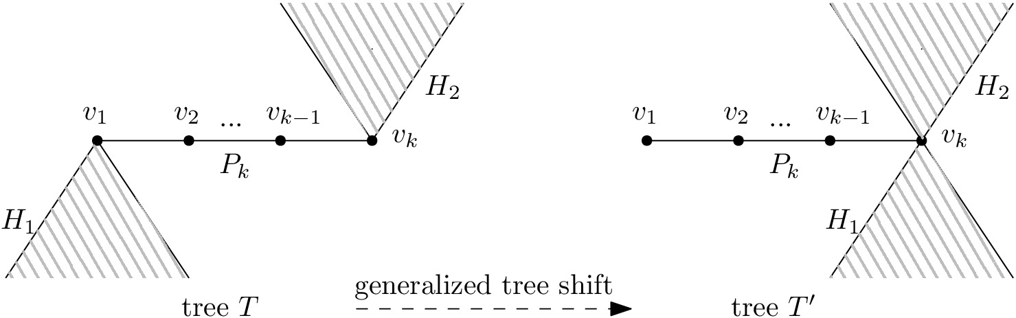
Figure 2. A generalized tree shift transforms a tree $T$ to anther tree $T^{\prime}$ (Definition 2.4).

Observe that the generalized tree shift increases the number of leaves by $1$ unless $T$ and $T^{\prime}$ are isomorphic graphs (when $v_{1}$ or $v_{k}$ is a leaf of $T$). Hence we may define the following poset.

Definition 2.5.

For $T,T^{\prime}\in{\mathcal{T}}_{n}$, we denote $T\leq T^{\prime}$ if $T^{\prime}$ can be obtained from $T$ by some generalized tree shifts. This gives a partial order on ${\mathcal{T}}_{n}$. We call it the Csikvári poset on ${\mathcal{T}}_{n}$. (See Figure 1.)

If a tree has two vertices that are not leaves, then one can increase the number of leaves by applying a generalized tree shift to the tree. This implies that the only maximal element of the Csikvári poset is the star. It is less trivial that the only minimal element is the path.

Proposition 2.6.

[4, Corollary 2.5] In the Csikvári poset $({\mathcal{T}}_{n},\leq)$, the tree $\text{Star}_{n}$ is the unique maximal element and the tree $\text{Path}_{n}$ is the unique minimal element.

3. Proof of Conjecture 1.2

When the tree $T^{\prime}$ covers $T$ in the Csikvári poset, we will prove the inequality $f(T^{\prime})\leq f(T)$ by factoring $f(T)-f(T^{\prime})$ into three polynomials with no negative coefficients (Proposition 3.2). To state this result, we need to define the following function.

Definition 3.1.

For a graph $G$ and a vertex $v$ of $G$, let $e(v)$ be the edge of $\text{Cone}(G)$ connecting the vertex $v$ and the apex $r$ of the cone. Note that $e(v)$ is a bridge if and only if there is no edge of $G$ incident to $v$. Define the function

$$g_{v}(G):=\begin{cases}T_{\text{Cone}(G)\backslash e(v)}(1,y),&\text{if there exists an edge of }G\text{ incident to }v,\\ 0,&\text{otherwise}.\end{cases}$$

Proposition 3.2.

For the two trees $T$ and $T^{\prime}$ in Definition 2.4, we have

$$f(T)-f(T^{\prime})=y\cdot g_{v_{1}}(H_{1})\cdot g_{v_{k}}(H_{2})\cdot g_{v_{1}}(P_{k}).$$

Consequently, $f(T^{\prime})\leq f(T)$.

Corollary 3.3.

Conjecture 1.2 holds.

Proof.

This is a direct consequence of Proposition 3.2 and the definition of Csikvári poset. ∎

Before we present the technical proof of Proposition 3.2, we introduce a notation and give an example first.

In this section, any path on $k$ vertices will be denoted by $P_{k}$ where the vertices are labeled by $v_{1},\cdots,v_{k}$ in order. Sometimes a formula or a sentence will involve two different paths where we use the same label for two different vertices; e.g. the paths $P_{2}$ and $P_{3}$ both have a vertex labeled by $v_{1}$. This abuse of notation should not cause any confusion in the context.

Example 3.4.

This example demonstrates Proposition 3.2. By direct computations, we have

$$g_{v_{1}}(P_{2})={\mathbf{T}}_{P_{2}}(1,y)=1,$$

$$g_{v_{2}}(P_{3})={\mathbf{T}}_{4\text{-cycle}}(1,y)=y+3,\text{ and}$$

$$g_{v_{1}}(P_{3})={\mathbf{T}}_{3\text{-cycle}}(1,y)=y+2.$$

Then we consider the data in Figure 1 and Table 1. The tree $T_{2}$ consists of a subtree $H_{1}=P_{3}$ with the distinguished vertex $v_{1}$, a subtree $H_{2}=P_{3}$ with the distinguished vertex $v_{2}$, and the path $P_{2}$ connecting the two distinguished vertices. The generalized tree shift transforms the tree $T_{2}$ into $T_{8}$. Then one can check that $f(T_{2})-f(T_{8})=y^{4}+7y^{3}+16y^{2}+12y=yg_{v_{1}}(P_{3})g_{v_{2}}(P_{3})g_{v_{1}}(P_{3})$.

Our main tool to prove Proposition 3.2 is what Csikvári called “General Lemma”.

Lemma 3.5.

(General Lemma)[5, Theorem 5.1] Let $f(G)$ be a graph polynomial in $y$. Assume there exists a graph polynomial $g_{v}(G)$ in $y$ whose inputs are a graph $G$ and a vertex of $G$ such that the following two conditions hold.

1. For any two graphs $G_{1}$ and $G_{2}$, we have

   $$f(G_{1}:G_{2})=c_{1}f(G_{1})f(G_{2})+c_{2}f(G_{1})g_{v}(G_{2})+c_{2}f(G_{2})g_{v}(G_{1})+c_{3}g_{v}(G_{1})g_{v}(G_{2}),$$

   where $c_{1},c_{2},c_{3}$ are rational functions of $y$ and $v$ is the identified vertex in $G_{1}:G_{2}$.

2. Denote

   $$q_{v}(G):=c_{2}f(G)+c_{3}g_{v}(G).$$

   We have that $q_{v_{1}}(P_{2})$ is not a zero polynomial.

Then the conclusion is

$$f(T)-f(T^{\prime})=\frac{g_{v_{1}}(P_{3})-g_{v_{2}}(P_{3})}{(q_{v_{1}}(P_{2}))^{2}}q_{v_{1}}(P_{k})q_{v_{1}}(H_{1})q_{v_{k}}(H_{2}),$$

where the trees $T$ and $T^{\prime}$ are as in Definition 2.4.

Although in our paper the function $f$ has been defined, the function $f$ in the lemma could be any graph polynomial. Csikvári called it the General Lemma because it was used to prove “$T<T^{\prime}\Rightarrow f(T)\leq f(T^{\prime})$” for several graph polynomials $f$ in [5]. One difficulty of applying the General Lemma is to find the function $g_{v}$, which we have given for our function $f$.

We will prove Proposition 3.2 by checking that our functions $f$ and $g_{v}$ satisfy the conditions in the General Lemma. We first introduce an auxiliary function

$$h_{v}(G):=T_{\text{Cone}(G)/e(v)}(1,y).$$

By the contraction-deletion relation of Tutte polynomials, we get

(1) $$f(G)=g_{v}(G)+h_{v}(G).$$

It is not hard to show that ${\mathbf{T}}_{G_{1}:G_{2}}(x,y)={\mathbf{T}}_{G_{1}}(x,y){\mathbf{T}}_{G_{2}}(x,y)$. Hence we have

(2) $$h_{v}(G_{1}:G_{2})=h_{v}(G_{1})h_{v}(G_{2}),$$

where $v$ is the identified vertex in $G_{1}:G_{2}$.

Lemma 3.6.

Let $v$ be the identified vertex in $G_{1}:G_{2}$. Then

$$f(G_{1}:G_{2})=f(G_{1})f(G_{2})-yg_{v}(G_{1})g_{v}(G_{2}).$$

Proof.

Observe that if there is no edge $e$ of $G_{1}$ incident to $v$, then we have $g_{v}(G_{1})=0$ and $f(G_{1}:G_{2})=f(G_{1})f(G_{2})$. Thus the desired equality holds.

Now we use induction on the number edges in $G_{1}$ to prove

$$f(G_{1})f(G_{2})-f(G_{1}:G_{2})=yg_{v}(G_{1})g_{v}(G_{2}).$$

The base case is that $G_{1}$ has no edge, which is covered by the observation above. For the inductive step, we may assume that there exists an edge $e$ of $G_{1}$ incident to $v$ (otherwise the case is covered by the observation). Let $e(v)$ be the edge of $\text{Cone}(G_{1})$ connecting the vertex $v$ and the apex of the cone.

Then by applying the contraction-deletion relation to the edge $e$ of $\text{Cone}(G_{1})$, we get

$$f(G_{1})=f(G_{1}\setminus e)+{\mathbf{T}}_{\text{Cone}(G_{1})/e}(1,y).$$

By further applying the contraction-deletion relation to the edge $e(v)$ of $\text{Cone}(G_{1})/e$ (which is one of the multiple edges produced by the contraction), we get

(3) $$f(G_{1})=f(G_{1}\setminus e)+f(G_{1}/e)+yh_{v}(G_{1}/e).$$

Similarly, by applying the contraction-deletion relation to the edge $e$ in $\text{Cone}(G_{1})\backslash e(v)$ and then applying Equation (1), we get

(4) $$\begin{split}g_{v}(G_{1})&=f(G_{1}/e)+g_{v}(G_{1}\setminus e)\\ &=g_{v}(G_{1}/e)+h_{v}(G_{1}/e)+g_{v}(G_{1}\setminus e).\end{split}$$

The following computation finishes the proof, where IH means the induction hypothesis.

$$\begin{split}&f(G_{1})f(G_{2})-f(G_{1}:G_{2})\\ \overset{(\ref{eq3})}{=}\ &(f(G_{1}\setminus e)+f(G_{1}/e)+yh_{v}(G_{1}/e))\cdot f(G_{2})-f(G_{1}\setminus e:G_{2})-f(G_{1}/e:G_{2})-yh_{v}(G_{1}/e:G_{2})\\ \overset{\text{IH}}{=}\ &yg_{v}(G_{1}\setminus e)g_{v}(G_{2})+yg_{v}(G_{1}/e)g_{v}(G_{2})+yh_{v}(G_{1}/e)f(G_{2})-yh_{v}(G_{1}/e:G_{2})\\ \overset{(\ref{eq2})}{=}\ &yg_{v}(G_{1}\setminus e)g_{v}(G_{2})+yg_{v}(G_{1}/e)g_{v}(G_{2})+yh_{v}(G_{1}/e)f(G_{2})-yh_{v}(G_{1}/e)h_{v}(G_{2})\\ \overset{(\ref{eq1})}{=}\ &yg_{v}(G_{1}\setminus e)g_{v}(G_{2})+yg_{v}(G_{1}/e)g_{v}(G_{2})+yh_{v}(G_{1}/e)g_{v}(G_{2})\\ \overset{(\ref{eq4})}{=}\ &yg_{v}(G_{1})g_{v}(G_{2}).\end{split}$$

∎

Proof of Proposition 3.2.

Consider applying the General Lemma with $c_{1}=1,c_{2}=0,c_{3}=-y$.

By Lemma 3.6, the first condition in the General Lemma holds. For the second condition, we have

$$q_{v}(G)=-yg_{v}(G),$$

and hence $q_{v_{1}}(P_{2})=-yg_{v_{1}}(P_{2})=-y\neq 0$ by Example 3.4. Thus the General Lemma can be applied in our setting, and a direct computation gives the desired equality. The inequality follows from the fact that the Tutte polynomials and hence $g_{v}(G)$ do not have negative coefficients. ∎

References

• [1] Matthew Baker and Farbod Shokrieh. Chip-firing games, potential theory on graphs, and spanning trees. J. Combin. Theory Ser. A, 120(1):164–182, 2013.
• [2] Olivier Bernardi. Tutte polynomial, subgraphs, orientations and sandpile model: new connections via embeddings. Electron. J. Combin., 15(1):Research Paper 109, 53, 2008.
• [3] Béla Bollobás and Mykhaylo Tyomkyn. Walks and paths in trees. J. Graph Theory, 70(1):54–66, 2012.
• [4] Péter Csikvári. On a poset of trees. Combinatorica, 30(2):125–137, 2010.
• [5] Péter Csikvári. On a poset of trees II. J. Graph Theory, 74(1):81–103, 2013.
• [6] A. K. Kelmans. On graphs with randomly deleted edges. Acta Math. Acad. Sci. Hungar., 37(1-3):77–88, 1981.
• [7] L. Lovász and J. Pelikán. On the eigenvalues of trees. Period. Math. Hungar., 3:175–182, 1973.
• [8] Criel Merino. Matroids, the Tutte polynomial and the chip firing game. PhD thesis, University of Oxford,, 1999.
• [9] Criel Merino. The chip firing game and matroid complexes. In Discrete models: combinatorics, computation, and geometry (Paris, 2001), volume AA of Discrete Math. Theor. Comput. Sci. Proc., pages 245–255. Maison Inform. Math. Discrèt. (MIMD), Paris, 2001.
• [10] Victor Reiner and Dorian Smith. Sandpile groups for cones over trees. arXiv preprint math/2402.15453, 2024.
• [11] Bo Zhou and Ivan Gutman. A connection between ordinary and Laplacian spectra of bipartite graphs. Linear Multilinear Algebra, 56(3):305–310, 2008.