On Holographic Vacuum Misalignment

Abstract

We develop a bottom-up holographic model that provides the dual description of a strongly coupled field theory, in which the spontaneous breaking of an approximate global symmetry yields the $SO(5)/SO(4)$ coset relevant to minimal composite-Higgs models. The gravity background is completely regular and smooth, and has an end of space that mimics confinement on the field theory side. We add to the gravity description a set of localised boundary terms, that introduce additional symmetry-breaking effects, capturing those that would result from coupling the dual strongly coupled field theory to an external, weakly coupled sector. Such terms encapsulate the gauging of a subgroup of the global $SO(5)$ symmetry of the dual field theory, as well as additional explicit symmetry-breaking effects. We show how to combine spurions and gauge fixing and how to take the appropriate limits, so as to respect gauge principles and avoid violations of unitarity.

The interplay of bulk and boundary-localised couplings leads to the breaking of the $SO(5)$ symmetry to either its $SO(4)$ or $SO(3)$ subgroup, via vacuum misalignment. In field theory terms, the model describes the spontaneous breaking of a $SO(4)$ gauge symmetry to its $SO(3)$ subgroup. We expose the implications of the higgsing phenomenon by computing the spectrum of fluctuations of the model, which we interpret in four-dimensional field-theory terms, for a few interesting choices of parameters. We conclude by commenting on the additional steps needed to build a realistic composite Higgs model.

I Introduction

The discovery of the Higgs boson Aad:2012tfa ; Chatrchyan:2012xdj provides a compelling argument for the study of composite Higgs models (CHMs) Kaplan:1983fs ; Georgi:1984af ; Dugan:1984hq : they extend the standard model (SM) of particle physics and can be tested by Large Hadron Collider (LHC) experiments. In this context, Higgs fields emerge as composite pseudo-Nambu-Goldstone bosons (PNGBs), in the weakly-coupled effective field theory (EFT) description of a more fundamental theory. Reviews can be found in Refs. Panico:2015jxa ; Witzel:2019jbe ; Cacciapaglia:2020kgq , and the summary tables in Refs. Ferretti:2013kya ; Ferretti:2016upr ; Cacciapaglia:2019bqz provide an interesting classification of possible fundamental field theory origins for CHMs, amenable (in principle) to non-perturbative numerical studies with lattice gauge theory.

The literature on model-building and phenomenological studies (see, e.g., Refs. Katz:2005au ; Barbieri:2007bh ; Lodone:2008yy ; Gripaios:2009pe ; Mrazek:2011iu ; Marzocca:2012zn ; Grojean:2013qca ; Barnard:2013zea ; Cacciapaglia:2014uja ; Ferretti:2014qta ; Arbey:2015exa ; Cacciapaglia:2015eqa ; vonGersdorff:2015fta ; Feruglio:2016zvt ; DeGrand:2016pgq ; Fichet:2016xvs ; Galloway:2016fuo ; Agugliaro:2016clv ; Belyaev:2016ftv ; Bizot:2016zyu ; Csaki:2017cep ; Chala:2017sjk ; Golterman:2017vdj ; Serra:2017poj ; Csaki:2017jby ; Alanne:2017rrs ; Alanne:2017ymh ; Sannino:2017utc ; Alanne:2018wtp ; Bizot:2018tds ; Cai:2018tet ; Agugliaro:2018vsu ; Cacciapaglia:2018avr ; Gertov:2019yqo ; Ayyar:2019exp ; Cacciapaglia:2019ixa ; BuarqueFranzosi:2019eee ; Cacciapaglia:2019dsq ; Cacciapaglia:2020vyf ; Dong:2020eqy ; Cacciapaglia:2021uqh ; Ferretti:2022mpy ; Banerjee:2022izw ; Cai:2022zqu ; Cacciapaglia:2024wdn ), is complemented by an expanding body of numerical lattice calculations, in theories with gauge group $SU(2)$ Hietanen:2014xca ; Detmold:2014kba ; Arthur:2016dir ; Arthur:2016ozw ; Pica:2016zst ; Lee:2017uvl ; Drach:2017btk ; Drach:2020wux ; Drach:2021uhl ; Bowes:2023ihh , $Sp(4)$ Bennett:2017kga ; Lee:2018ztv ; Bennett:2019jzz ; Bennett:2019cxd ; Lucini:2021xke ; Bennett:2021mbw ; Bennett:2022yfa ; Lee:2022xbp ; Bennett:2023wjw ; Bennett:2023rsl ; Bennett:2023gbe ; Mason:2023ixv ; Bennett:2023mhh ; Bennett:2023qwx ; Hsiao:2023nyn ; Bennett:2024cqv ; Bennett:2024wda ; Dengler:2024maq and $SU(4)$ Ayyar:2017qdf ; Ayyar:2018zuk ; Ayyar:2018ppa ; Ayyar:2018glg ; Cossu:2019hse ; Shamir:2021frg ; Lupo:2021nzv ; DelDebbio:2022qgu ; Hasenfratz:2023sqa . Results for the $SU(3)$ theory with $N_{f}=8$ Dirac fermions Aoki:2014oha ; Appelquist:2016viq ; Aoki:2016wnc ; Gasbarro:2017fmi ; Appelquist:2018yqe ; LSD:2023uzj ; LatticeStrongDynamics:2023bqp ; Ingoldby:2023mtf have been reinterpreted in terms of new CHMs, embedded in the dilaton EFT framework Appelquist:2020bqj ; Appelquist:2022qgl —see also Refs. Vecchi:2015fma ; Ma:2015gra ; BuarqueFranzosi:2018eaj . But the microscopic origin of CHMs with minimal $SO(5)/SO(4)$ coset is more obscure—see for instance Ref. Caracciolo:2012je .

Central to the CHM model-building programme is the absence of new physics signals in direct and indirect searches, indicating that the scale of new phenomena, $f$, is higher than the electroweak scale, $v$. This little hierarchy originates in the strong-coupling dynamics, as a consequence of small destabilising perturbations of the vacuum, due to perturbative, weak interactions with an external sector. Rephrasing the title of the classical work in Ref. Peskin:1980gc , the electroweak scale is suppressed by what is called the vacuum misalignment angle, $\theta\sim v/f\ll 1$—see, e.g., Sect. 2.2.1 of Ref. Cacciapaglia:2020kgq , and references therein. In practical terms, phenomenological constraints can be satisfied with a rather modest suppression of $\theta$, and only a moderate tuning of parameters, which adds to the appeal of CHMs. Yet, computing $\theta$ from first principles requires non-perturbative methods.

A new alternative avenue for the study of non-perturbative phenomena opened within the context of string theory and supergravity, with the discovery of gauge-gravity dualities (holography) Maldacena:1997re ; Gubser:1998bc ; Witten:1998qj ; Aharony:1999ti . The strongly coupled regime of special field theories admits an equivalent description as a weakly coupled gravity theory in higher dimensions. For example, type-IIA supergravity backgrounds, in which the geometry includes a shrinking internal circle, provide a holographic description of linear confinement in Yang-Mills theories Witten:1998zw , allowing to study glueball spectra Brower:2000rp , chiral symmetry breaking Karch:2002sh ; Babington:2003vm , and masses of mesons Sakai:2004cn ; Sakai:2005yt ; Kruczenski:2003be ; Nunez:2003cf ; Erdmenger:2007cm . Also within type IIB supergravity, backgrounds exist in which a whole portion of internal space, the base of the conifold Candelas:1989js , shrinks to zero size, giving rise to a rich phenomenology Klebanov:1998hh ; Klebanov:2000nc ; Klebanov:2000hb ; Chamseddine:1997nm ; Maldacena:2000yy ; Butti:2004pk , including the possibility of a light dilaton Elander:2009pk ; Elander:2012yh ; Elander:2014ola ; Elander:2017cle ; Elander:2017hyr . Simpler bottom-up holographic models dispense with the microscopic origin of the gravity theory, complementing lattice explorations of CHMs Erdmenger:2020lvq ; Erdmenger:2020flu ; Elander:2020nyd ; Elander:2021bmt ; Erdmenger:2023hkl ; Erdmenger:2024dxf . It is indeed in this context that CHMs based on the minimal $SO(5)/SO(4)$ coset have been first developed Contino:2003ve ; Agashe:2004rs ; Agashe:2005dk ; Agashe:2006at ; Contino:2006qr ; Falkowski:2008fz ; Contino:2010rs ; Contino:2011np .

A holographic CHM derived from a fundamental gravity theory more accurately predicts the properties of composite states. A step towards such a construction was pursued in Ref. Elander:2021kxk , by exploiting the classical work on $S^{4}$ compactifications of maximal supergravity in $D=11$ dimensions Pilch:1984xy ; Nastase:1999cb ; Pernici:1984xx ; Pernici:1984zw ; Cvetic:1999xp ; Lu:1999bc ; Cvetic:2000ah ; Samtleben:2005bp , its reductions to $D=7$ dimensions, and its symmetry-breaking backgrounds Campos:2000yu ; Elander:2013jqa , which lead to the appearance of the minimal $SO(5)/SO(4)$ coset. Reference Elander:2021kxk is the first exploratory work, in the larger space of supergravity theories, that features a variety of different coset structures and gauge symmetries—a useful review on gauged supergravities is Ref. Samtleben:2008pe .

In this paper, we present the next stage of development of the minimal realisation of holographic CHMs. Our motivation for embarking on this task is that the ambitious programme of embedding a holographic CHM within the fully rigorous context of top-down holography requires additional preliminary work on the formalism, before making contact with model-building and phenomenological aspects. In the next subsection, we elaborate on why this is so, and clarify what are the objectives of the present investigation, in which we focus on developing and testing the formalism with a semi-realistic bottom-up model. The simpler construction we propose captures much of the physically interesting aspects of the CHM programme and is interesting and useful in itself, as a stand-alone model.

I.1 A roadmap towards top-down holographic composite Higgs

The complete construction of a top-down holographic CHM would involve the following steps.

• Identify a fundamental gravity theory (the low energy description of which may be given by supergravity), providing the dual description of a field theory in which spontaneous symmetry breaking involves the $G/H$ coset relevant to a CHM of interest.

• Find regular gravity solutions that holographically describe confinement in the dual four-dimensional field theory.

• Compute the (holographically renormalised) free energy, and the spectrum of fluctuations, dual to the bound states of the field theory. Verify the absence of tachyons or other signals of instability.

• Extend the gravity theory so that in the field-theory interpretation a subgroup of the global symmetry is gauged, with coupling strength weak enough to allow for the perturbative treatment to be viable.

• Extend the gravity theory to implement explicit breaking of the field-theory global symmetry, compatibly with gauge principles and unitarity. Additional auxiliary fields (spurions) may be needed.

• Perform a vacuum alignment analysis, within the gravity theory, to determine the field-theory vacuum structure.

• Verify that no pathologies emerge in the mass spectrum in the presence of symmetry-breaking terms.

• Couple the theory to standard-model fields, and identify viable regions of parameter space. This step might also involve the introduction of top partial compositeness Kaplan:1991dc (see also the discussions in Refs. Grossman:1999ra ; Gherghetta:2000qt ; Lodone:2008yy ; Chacko:2012sy ; Grojean:2013qca ).

Points 1), 2), and 3) are addressed in Ref. Elander:2021kxk ; the minimal $SO(5)/SO(4)$ coset, relevant to CHMs, emerges within maximal supergravity in $D=7$ dimensions, which lifts to type-IIA supergravity in $D=10$ dimensions. The spectrum of fluctuations of bosons, upon compactification on a 2-torus, is computed Elander:2021kxk for backgrounds dual to a confining, four-dimensional field theory, by exploiting the formalism in Refs. Bianchi:2003ug ; Berg:2005pd ; Berg:2006xy ; Elander:2009bm ; Elander:2010wd —see also Refs. Elander:2014ola ; Elander:2017cle ; Elander:2017hyr ; Elander:2020csd ; Elander:2020fmv ; Roughley:2021suu ; Elander:2018aub .

A simpler bottom-up model, written in $D=6$ dimensions Elander:2022ebt ; Elander:2023aow , readdresses points 1), 2), and 3), with several technical advantages: the spectrum is simpler, the action contains only essential fields, with canonical normalisations and minimal interactions. The model is free from the complexities descending from supersymmetry in higher dimensions, while retaining the essential features of interest (confinement and symmetry breaking).

In this paper, we address points 4), 5), 6), and 7) for the bottom-up model in Refs. Elander:2022ebt ; Elander:2023aow , in a way that can be generalised to more complicated cosets and geometries. The $SO(4)$ subgroup of the (field-theory) global symmetry is gauged weakly, and a spurion field introduces explicit breaking of $SO(5)$ to $SO(4)$. We discuss how to implement gauge-fixing within this setting. Both new features are controlled by a boundary-localised action in the gravity theory. The interplay with the background dynamics—vacuum (mis)alignment—determines whether the mass spectra display $SO(5)\rightarrow SO(4)$ breaking (and unbroken gauged $SO(4)$) or $SO(5)\rightarrow SO(3)$ breaking (with the gauged $SO(4)$ subgroup higgsed to $SO(3)$).

In contrast to the earliest bottom-up models Contino:2010rs , the smooth and regular geometry deviates substantially from AdS, and the mass gap is due to the existence of an endpoint of the radial (holographic) direction Witten:1998zw , while symmetry breaking is triggered by bulk fields, similar to so-called soft-wall models previously considered in the literature Karch:2006pv ; Falkowski:2008fz ; Batell:2008me . For these reasons, some formal developments warrant special attention, and are the main topic of this paper. The consequences of holographic vacuum (mis)alignment can be illustrated within this simple model to highlight general results that apply to a large variety of holographic realisations of CHMs. We detail necessary, unconventional yet rigorous elements of the formalism, and subtleties in the (weak) gauging of the symmetry that generalise holographic renormalisation Bianchi:2001kw ; Skenderis:2002wp ; Papadimitriou:2004ap . We defer the construction of a realistic bottom-up holographic CHM EWSB , obtained by gauging the standard-model $SU(2)_{L}\times U(1)_{Y}\subset SO(4)\times U(1)_{B-L}$—the Abelian factor is related to baryon, $B$, and lepton, $L$, quantum numbers—and by adding fermions, either in the bulk or localised at the boundary.

The paper is organised as follows. In Sect. II, we introduce the six-dimensional bottom-up gravity model of interest and its $SO(5)$ gauge symmetry. The profile of a bulk scalar field breaks such symmetry. A shrinking circle in the geometry mimics confinement on the field theory side. We introduce the elements needed to make the exposition self-contained, and fix notation and conventions, but dispense with details, that may be found in Refs. Elander:2022ebt ; Elander:2023aow . We digress in Sect. III, to discuss a rather general description, in effective field theory terms, of non-linear sigma models based on the $SO(5)/SO(4)$ coset, in particular in order to clarify the subtle differences between gauge and global symmetries, and explicit and spontaneous symmetry breaking. In Sect. IV, we return to the gravity theory. In order to weakly gauge, in the dual field theory, an $SO(4)$ subgroup of the $SO(5)$ global symmetry, we add appropriate boundary terms to the gravity description. We discuss the implications for the vacuum of the theory, and the resulting symmetry breaking pattern, in Sect. V. In Sect. VI, we display the mass spectrum of fluctuations of the gravity theory, which we interpret as bound states of the dual field theory. We outline further work that we leave for future investigations in Sect. VII. We relegate to the Appendix extensive amounts of technical details.

II The gravity model

The bottom-up holographic model of interest Elander:2023aow is built by coupling gravity in $D=6$ dimensions to a bulk scalar field, $\mathcal{X}$, transforming in the vector, real representation, $5$, of a gauged $SO(5)$ symmetry. One of the non-compact space-time dimensions, denoted as $\rho$, is interpreted as the holographic direction. We restrict attention to background solutions with asymptotically AdS₆ geometry, for large values of the holographic direction—the ultra-violet (UV) regime of the (putative) dual field theory. Another one of the space-like dimensions is compactified on a circle that shrinks smoothly to zero size at a finite value, $\rho=\rho_{o}$, of the holographic direction—the infra-red (IR) regime. The presence of an end to the space introduces a mass gap in the dual field theory interpretation, mimicking the effect of confinement in the four-dimensional field theory. A subclass of backgrounds exists in which $\mathcal{X}$ acquires a non-trivial profile, breaking spontaneously the $SO(5)$ gauge symmetry of the gravity theory to its $SO(4)$ subgroup.

II.1 Six-dimensional action

Table 1: Field content of the model, organised in terms of irreducible representations of the symmetries in $D=6$ dimensions ($SO(5)$ multiplets), as well as $D=5$ dimensions ($SO(4)$ multiplets, assuming $\langle{\mathcal{X}}\rangle\neq 0$), and $D=4$ dimensions ($SO(3)$ multiplets, assuming $\langle\vec{\pi}\rangle\neq 0$). In the case of the language in $D=4$ dimensions, we indicate the field content in terms of the massive representations of the Poincaré group, and keep into account the degrees of freedom of gauge-invariant combinations only. The irreducible representations for which we indicate $N_{\rm dof}=-$ refer to cases where the degrees of freedom have been included in propagating degrees of freedom of other fields, to build gauge invariant combinations—for explanations, see the body of the paper. For space-time indexes, $\hat{M}=0,\,1,\,2,\,3,\,5,\,6$, while $M=0,\,1,\,2,\,3,\,5$, and $\mu=0,\,1,\,2,\,3$. For indexes of the internal symmetry, $\alpha,\beta=1,\,\cdots,\,5$, while $A=1,\,\cdots,\,10$, $\hat{A}=1,\,\cdots,\,4$, and $\bar{A}=6,\,\cdots,\,10$. When the $SO(4)$ symmetry is broken to $SO(3)$, we use indexes $\hat{\cal A}=1,\,2,\,3$, $\tilde{\cal A}=5,\,6,\,7$, and $\bar{\cal A}=8,\,9,\,10$.

$D=6$, $SO(5)$,			$D=5$, $SO(4)$,			$D=4$, $SO(3)$,
massless irreps.			massless irreps.			massive irreps.
Field	$SO(5)$	$N_{\rm dof}$	Field	$SO(4)$	$N_{\rm dof}$	Field	$SO(3)$	$N_{\rm dof}$
$\hat{g}_{\hat{M}\hat{N}}$	$1$	$9$	$g_{MN}$	$1$	$5$	$g_{\mu\nu}$	$1$	$5$
						$g_{\mu 5}$	$1$	$-$
						$g_{55}$	$1$	$-$
			$\chi_{M}$	$1$	$3$	$\chi_{\mu}$	$1$	$3$
						$\chi_{5}$	$1$	$-$
			$\chi$	$1$	$1$	$\chi$	$1$	$1$
${\mathcal{X}}_{\alpha}$	$5$	$5$	$\phi$	$1$	$1$	$\phi$	$1$	$1$
			$\pi^{\hat{A}}$	$4$	$4$	$\pi^{\hat{\cal A}}$	$3$	$3$
						$\pi^{4}$	$1$	$1$
${\cal A}_{\hat{M}\,\alpha}{}^{\beta}$	$10$	$40$	${\cal A}_{M}^{\,\,\,\hat{A}}$	$4$	$12$	${\cal A}_{\mu}^{\,\,\,\hat{\cal A}}$	$3$	$9$
						${\cal A}_{\mu}^{\,\,\,4}$	$1$	$3$
						${\cal A}_{5}^{\,\,\,\hat{\cal A}}$	$3$	$-$
						${\cal A}_{5}^{\,\,\,4}$	$1$	$-$
			${\cal A}_{6}^{\,\,\,\hat{A}}$	$4$	$4$	${\cal A}_{6}^{\,\,\,\hat{\cal A}}$	$3$	$3$
						${\cal A}_{6}^{\,\,\,4}$	$1$	$1$
			${\cal A}_{M}^{\,\,\,\bar{A}}$	$6$	$18$	${\cal A}_{\mu}^{\,\,\,\tilde{\cal A}}$	$3$	$9$
						${\cal A}_{\mu}^{\,\,\,\bar{\cal A}}$	$3$	$9$
						${\cal A}_{5}^{\,\,\,\tilde{\cal A}}$	$3$	$-$
						${\cal A}_{5}^{\,\,\,\bar{\cal A}}$	$3$	$-$
			${\cal A}_{6}^{\,\,\,\bar{A}}$	$6$	$6$	${\cal A}_{6}^{\,\,\,\tilde{\cal A}}$	$3$	$3$
						${\cal A}_{6}^{\,\,\,\bar{\cal A}}$	$3$	$3$
$P_{5}{}_{\alpha}$	5	5	$P_{5}{}_{\hat{A}}$	4	4	$P_{5}{}_{\hat{\cal A}}$	3	3
						$P_{5}{}_{4}$	1	1
			$P_{5}{}_{5}$	1	1	$P_{5}{}_{5}$	1	1

We review the essential features of the model to keep the presentation self-contained and explain the notation—see Table 1—without discussing details that can be found in Ref. Elander:2022ebt , in respect to which we rescale the action in $D=6$ dimensions by an overall factor of $\frac{1}{2\pi}$, to lighten the notation in matching it to lower dimensions:

$$\mathcal{S}_{6}^{(bulk)} =\frac{1}{2\pi}\int\mbox{d}^{6}x\sqrt{-\hat{g}_{6}}\,\bigg{\{}\frac{\mathcal{R}_{6}}{4}-\frac{1}{2}\hat{g}^{\hat{M}\hat{N}}\left(D_{\hat{M}}\mathcal{X}\right)^{T}D_{\hat{N}}\mathcal{X}-\mathcal{V}_{6}(\mathcal{X})-\frac{1}{2}{\rm Tr}\left[\hat{g}^{\hat{M}\hat{P}}\hat{g}^{\hat{N}\hat{Q}}\mathcal{F}_{\hat{M}\hat{N}}\mathcal{F}_{\hat{P}\hat{Q}}\right]\bigg{\}}\,.$$ (1)

The six-dimensional space-time indexes are denoted by $\hat{M}=0,1,2,3,5,6$. The six-dimensional metric, $\hat{g}_{\hat{M}\hat{N}}$, has determinant $\hat{g}_{6}$, and signature mostly $+$. The six-dimensional Ricci scalar is denoted as $\mathcal{R}_{6}$.

The components, ${\mathcal{X}}_{\alpha}$, of the scalar transforming in the $5$ of $SO(5)$, are labelled by Greek indexes, $\alpha=1,\,\cdots,\,5$. The $SO(5)$ gauge field is denoted by $\mathcal{A}_{\hat{M}}$. The covariant derivatives are defined as follows:

$$\left(D_{\hat{M}}\mathcal{X}\right)_{\alpha} \equiv\partial_{\hat{M}}\mathcal{X}_{\alpha}+i{g}\mathcal{A}_{\hat{M}\,\alpha}{}^{\beta}\mathcal{X}_{\beta}\,,$$ (2)

and the field-strength tensors are

$$\mathcal{F}_{\hat{M}\hat{N}\,\alpha}{}^{\beta} \equiv 2\left(\partial_{[\hat{M}}\mathcal{A}_{\hat{N}]\,\alpha}{}^{\beta}+i{g}\mathcal{A}_{[\hat{M}\,\alpha}{}^{\gamma}\mathcal{A}_{\hat{N}]\,\gamma}{}^{\beta}\right)\,,$$ (3)

where antisymmetrisation is defined as $[n_{1}n_{2}]\equiv\frac{1}{2}\left(n_{1}n_{2}-n_{2}n_{1}\right)$. The bulk gauge coupling, ${g}$, is a free parameter. One can, equivalently, write covariant derivatives and field-strength tensors in terms of the generators, $t^{A}$ ($A=1,\cdots,10$) of $SO(5)$, normalised so that ${\rm Tr}(t^{A}t^{B})=\frac{1}{2}\delta^{AB}$. We exhibit an explicit basis for these generators in Appendix A.

The bulk scalar potential, $\mathcal{V}_{6}(\mathcal{X})$, is manifestly $SO(5)$ invariant, as it depends only on the combination $\phi\equiv\sqrt{\mathcal{X}^{T}\mathcal{X}}$. With the convenient choice of superpotential, ${\mathcal{W}}_{6}$, adopted in Ref. Elander:2023aow :

$$\mathcal{W}_{6}\equiv-2-\frac{\Delta}{2}{\mathcal{X}}^{T}{\mathcal{X}}\,=\,-2-\frac{\Delta}{2}\phi^{2}\,,$$ (4)

one finds the potential to be the following:

$$\mathcal{V}_{6}\equiv\frac{1}{2}\sum_{\alpha}\left(\frac{\partial{\mathcal{W}}_{6}}{\partial{\mathcal{X}}_{\alpha}}\right)^{2}-\frac{5}{4}\mathcal{W}_{6}^{2}=-5-\frac{\Delta(5-\Delta)}{2}\phi^{2}-\frac{5\Delta^{\chi}}{16}\phi^{4}\,,$$ (5)

We adopt this form of the potential, $\mathcal{V}_{6}$, for its simplicity, and note that its origin in terms of a superpotential, $\mathcal{W}_{6}$, does not make the model supersymmetric: there are no fermionic fields, nor do the backgrounds discussed in this paper originate from solving first-order equations derived from $\mathcal{W}_{6}$.

The general configuration of the scalar field, $\mathcal{X}$, can be parametrised as

$$\mathcal{X} \equiv\exp\left[2i\sum_{\hat{A}}\pi^{\hat{A}}t^{\hat{A}}\right]\,\mathcal{X}_{0}\,\phi\,,\qquad{\rm where}\qquad\mathcal{X}_{0}\equiv(0,0,0,0,1)^{T}\,,$$ (6)

with ${\hat{A}}=1,\,\cdots,\,4$, labelling the generators of the $SO(5)/SO(4)$ coset. If $\langle\phi\rangle\neq 0$, one can also write $\mathcal{X}$ explicitly, as

$$\mathcal{X}=\phi\left(\sin(|\vec{\pi}|)\frac{\vec{\pi}}{|\vec{\pi}|},\cos(|\vec{\pi}|)\right)^{T}\,,$$ (7)

in terms of the four PNGBs, $\vec{\pi}=(\pi^{1},\,\pi^{2},\,\pi^{3},\,\pi^{4})$, spanning the $SO(5)/SO(4)$ coset.

II.2 Dimensional reduction and background solutions

We find it convenient to write the background solutions of interest by first dimensionally reducing the theory to $D=5$ dimensions. The sixth dimension is a circle, parameterised by an angle, $0\leq\eta<2\pi$. The metric ansatz is

$$\mbox{d}s_{6}^{2} =e^{-2\chi}\mbox{d}s_{5}^{2}+e^{6\chi}\left(\mbox{d}\eta+\chi_{M}\mbox{d}x^{M}\right)^{2}\,,$$ (8)

where the five-dimensional space-time index is $M=0,1,2,3,5$, and the five-dimensional metric is

$$\mbox{d}s_{5}^{2}=\mbox{d}r^{2}+e^{2A(r)}\mbox{d}x_{1,3}^{2}=e^{2\chi(\rho)}\mbox{d}\rho^{2}+e^{2A(\rho)}\mbox{d}x_{1,3}^{2}\,.$$ (9)

In the background, the warp factor, $A$, as well as the scalars, $\mathcal{X}_{\alpha}$ and $\chi$, depend only on the holographic coordinate, $\rho$, whereas $\mathcal{A}_{6}=0$, and $\mathcal{A}_{M}=0=\chi_{M}$. The background equations of motion for $\mathcal{X}_{\alpha}(\rho)$, $\chi(\rho)$, and $A(\rho)$ are given by

$$\partial_{\rho}^{2}\mathcal{X}_{\alpha}+(4\partial_{\rho}A-\partial_{\rho}\chi)\partial_{\rho}\mathcal{X}_{\alpha} =\frac{\partial{\mathcal{V}_{6}}}{\partial{\mathcal{X}}_{\alpha}}\,,$$ (10)

$$\partial_{\rho}^{2}\chi+(4\partial_{\rho}A-\partial_{\rho}\chi)\partial_{\rho}\chi =-\frac{\mathcal{V}_{6}}{3}\,,$$ (11)

$$3(\partial_{\rho}A)^{2}-\frac{1}{2}\partial_{\rho}\mathcal{X}_{\alpha}\partial_{\rho}\mathcal{X}_{\alpha}-3(\partial_{\rho}\chi)^{2} =-\mathcal{V}_{6}\,.$$ (12)

In Refs. Elander:2022ebt ; Elander:2023aow , radial profiles of the background fields, $\phi(\rho)$, $\chi(\rho)$, and $A(\rho)$, satisfying Eqs. (10–12), and resulting in regular geometries, are identified and referred to (with some abuse of language) as confining solutions. We repeat here their IR expansions, that can be used to construct the full solutions numerically, by setting up the boundary conditions in the vicinity of the coordinate, $\rho=\rho_{o}$, at which the space ends, and by expanding in powers of the small difference, $\rho-\rho_{o}$:

$$\phi(\rho) = \phi_{I}-\frac{1}{16}\Delta\phi_{I}\left(20+\Delta\left(5\phi_{I}^{2}-4\right)\right)(\rho-\rho_{o})^{2}+\mathcal{O}\left((\rho-\rho_{o})^{4}\right)\,,$$ (13)

$$\chi(\rho) = \chi_{I}+\frac{1}{3}\log(\rho-\rho_{o})+\frac{1}{288}\left(-80+8\left(\Delta-5\right)\Delta\phi_{I}^{2}-5\Delta^{\chi}\phi_{I}^{4}\right)(\rho-\rho_{o})^{2}+O\left((\rho-\rho_{o})^{4}\right)\,,$$ (14)

$$A(\rho) = A_{I}+\frac{1}{3}\log(\rho-\rho_{o})+\frac{7}{576}\left(80+\Delta\phi_{I}^{2}\left(40+\Delta\left(5\phi_{I}^{2}-8\right)\right)\right)(\rho-\rho_{o})^{2}+\mathcal{O}\left((\rho-\rho_{o})^{4}\right)\,.$$ (15)

Here, $\phi_{I}$, $\chi_{I}$, and $A_{I}$ are integration constants, and we set $\chi_{I}=0$ to avoid a conical singularity in the plane described in polar coordinates by $(\rho,\eta)$. In those solutions, $\langle\vec{\pi}\rangle=0$. In this paper, we adopt the same solutions for $\phi(\rho)$, $\chi(\rho)$, and $A(\rho)$, but we allow for $\langle\vec{\pi}\rangle\neq 0$, as we shall see in Sect. IV.

We also reproduce here the UV expansions for the background solutions, written in terms of $z\equiv e^{-\rho}$. These depend non-trivially on the value of $\Delta$. Defining $\Delta_{J}={\rm min}\left(\Delta,\,5-\Delta\right)$, and $\Delta_{V}=5-\Delta_{J}$, they take the generic form

$$\phi(z) = \phi_{J}z^{\Delta_{J}}\,+\,\cdots\,+\phi_{V}z^{\Delta_{V}}\,+\,\cdots\,,$$ (16)

$$\chi(z) = \chi_{U}-\frac{1}{3}\log(z)\,+\,\cdots+({\chi_{5}}+\cdots)z^{5}\,+\,\cdots\,,$$ (17)

$$A(z) = A_{U}-\frac{4}{3}\log(z)\,+\,\cdots\,.$$ (18)

The integration constants, $\phi_{J}$ and $\phi_{V}$, appear at leading and subleading order, respectively. Another integration constant, $\chi_{5}$, is related to the radial dependence of the size of the compactified circle. Finally, $A_{U}$ and $\chi_{U}$ only appear trivially, as overall factors, and in the following, we set them to zero without loss of generality—see Ref. Elander:2020ial .

The circle reduction of the six-dimensional model leads to the following five-dimensional bulk action Elander:2023aow :

$$\mathcal{S}_{5}^{(bulk)} = \int\mbox{d}^{5}x\sqrt{-g_{5}}\,\left\{\rule{-2.84544pt}{21.33955pt}\right.\frac{R}{4}-3g^{MN}\partial_{M}\chi\partial_{N}\chi-\frac{g^{MN}}{2}\left(D_{M}\mathcal{X}\right)^{T}(D_{N}\mathcal{X})-g^{MN}e^{-6\chi}{\rm Tr}\left[D_{M}\mathcal{A}_{6}\frac{}{}D_{N}\mathcal{A}_{6}\right]$$

$$-e^{-2\chi}\mathcal{V}_{6}-\frac{1}{2}g^{2}e^{-8\chi}\mathcal{X}^{T}\mathcal{A}_{6}^{2}\mathcal{X}-\frac{1}{16}e^{8\chi}g^{MP}g^{NQ}F^{(\chi)}_{MN}F^{(\chi)}_{PQ}-\frac{1}{2}e^{2\chi}{\rm Tr}\left[g^{MP}g^{NQ}\mathcal{F}_{MN}\mathcal{F}_{PQ}\right]$$

$$-ig\,g^{MN}\chi_{M}\mathcal{X}^{T}\mathcal{A}_{6}D_{N}\mathcal{X}-2e^{2\chi}g^{MN}g^{OP}\chi_{M}{\rm Tr}\left(\mathcal{F}_{NO}D_{P}\mathcal{A}_{6}\right)-\frac{1}{2}g^{2}g^{MN}\chi_{M}\chi_{N}\mathcal{X}^{T}\mathcal{A}_{6}^{2}\mathcal{X}$$

$$+e^{2\chi}g^{MP}g^{NQ}\chi_{M}\chi_{N}{\rm Tr}\left(D_{P}\mathcal{A}_{6}D_{Q}\mathcal{A}_{6}\right)-e^{2\chi}g^{MN}g^{PQ}\chi_{M}\chi_{N}{\rm Tr}\left(D_{P}\mathcal{A}_{6}D_{Q}\mathcal{A}_{6}\right)\left.\rule{-2.84544pt}{21.33955pt}\right\}\,.$$

We exhibit this action purely in the interest of completeness, and anticipate that, in Sect. IV, we will rewrite it, in a form more suitable for the computation of spectra, by expanding it in powers of small fluctuations, and approximating it by retaining only quadratic order in said fluctuations.

III Effective Field Theory

Figure 1: Moose diagram representing the $SO(5)/SO(4)$ EFT—figure generated with axodraw2 Collins:2016aya .

The purpose of this subsection is to clarify, within the language of four-dimensional effective field theories, the role of explicit and spontaneous breaking of internal continuous symmetries. In particular, we want to expose differences and commonalities between the treatment of global and local symmetries. We occasionally recall definitions and notational conventions introduced earlier on in such a way that this short section is self-contained. It should be stressed that this section does not provide the precise EFT, low-energy description of the theory of interest in the rest of the paper, and we do not attempt to match the two, as doing so would go beyond current purposes.

We start by writing the non-linear sigma-model Lagrangian density capturing the long distance dynamics associated with the spontaneous breaking of a gauged $SO(5)$ symmetry to its $SO(3)$ subgroup. The field content consists of two (real) fields, $\Sigma$ and ${\Xi}$, both transforming in the $5$ of $SO(5)$, so that, under the action of a symmetry transformation:

$$(\Sigma,\,{\Xi}) \rightarrow (U\,\Sigma,\,U\,{\Xi})\,,$$ (20)

where $U\in SO(5)$ is a group element (a special, orthogonal, real matrix).

As stated in Sect. II, we denote as $t^{A}$ the generators of $SO(5)$, normalised so that ${\rm Tr}\,(t^{{A}}t^{B})=\frac{1}{2}\delta^{AB}$, and use, where appropriate, the choice of basis in Appendix A. We gauge the $SO(5)$ symmetry, by defining $A_{\mu}\equiv\sum_{A}A_{\mu}^{{A}}t^{{A}}$, so that the covariant derivatives are

$$D_{\mu}\Sigma \equiv \partial_{\mu}\Sigma\,+\,i\,g\,A_{\mu}\Sigma\,,$$ (21)

$$D_{\mu}{\Xi} \equiv \partial_{\mu}{\Xi}\,+\,i\,g\,A_{\mu}{\Xi}\,,$$ (22)

$$F_{\mu\nu} \equiv \partial_{\mu}A_{\nu}-\partial_{\nu}A_{\mu}+i\,g\left[A_{\mu},\,A_{\nu}\right]\,,$$ (23)

with $g$ the (weak) gauge coupling strength. The $SO(5)$-invariant Lagrangian density is the following:

$${\cal L}_{SO(5)} \equiv \frac{f^{2}}{2}\left[\left(D_{\mu}\Sigma\right)^{T}\left(D^{\mu}\Sigma\right)\right]\,+\,\frac{\kappa^{2}f^{2}}{2}\left[\left(D_{\mu}{\Xi}\right)^{T}\left(D^{\mu}{\Xi}\right)\right]$$

$$\,-\,\frac{1}{2}{\rm Tr}\left[F_{\mu\nu}F^{\mu\nu}\right]\,+\,{(1-\tilde{\kappa}^{2})}{}\,{\Xi}^{T}\,F_{\mu\nu}\,F^{\mu\nu}\,{\Xi}$$

$$\,-\,\lambda_{\Sigma}f^{4}\left(\Sigma^{T}\Sigma-1\right)^{2}\,-\,\lambda_{\Xi}f^{4}\left({\Xi}^{T}{\Xi}-1\right)^{2}\,-\,{\cal V}_{SO(5)}(\Sigma,\,\Xi)\,,$$

where $f$ is the scale of the theory, and the couplings are denoted by $\kappa$, $\tilde{\kappa}$, $\lambda_{\Sigma}$, and $\lambda_{\Xi}$. We will return to the $SO(5)$-invariant potential, ${\cal V}_{SO(5)}(\Sigma,\,\Xi)$, and the important physical parameters it encodes, in due course.

We require the divergence of the couplings $\lambda_{\Sigma}\rightarrow+\infty$ and $\lambda_{{\cal V}}\rightarrow+\infty$, hence enforcing the non-linear constraints $\Sigma^{T}\Sigma=1={\Xi}^{T}{\Xi}$. Both these vacuum expectation values (VEVs) break $SO(5)$ to a $SO(4)$ subgroup, which may differ in the two cases. We conventionally adapt our choice of basis for $SO(5)$ so that we denote as $t^{\bar{A}}$, with $\bar{A}=5,\,\cdots,\,10$, the generators that obey the relation $t^{\bar{A}}\,\langle{\Xi}\rangle=0$, and generate an $SO(4)$ subgroup of $SO(5)$, while $t^{\hat{A}}$, with $\hat{A}=1,\,\cdots,\,4$, are the four generators describing the corresponding $SO(5)/SO(4)$ coset. We then define $\varsigma=\sum_{\hat{A}}\varsigma^{\hat{A}}t^{\hat{A}}$ and $\varrho=\sum_{\hat{A}}\varrho^{\hat{A}}t^{\hat{A}}$, to parameterise the two scalar fields as

$$\Sigma = e^{\frac{2i}{f}{\varsigma}}\,\left(\begin{array}[]{c}0\cr 0\cr 0\cr 0\cr 1\end{array}\right)\,,\qquad{\rm and}\qquad{\Xi}\,=\,e^{\frac{2i}{f}\varrho}\,\left(\begin{array}[]{c}0\cr 0\cr 0\cr 0\cr 1\end{array}\right)\,.$$ (35)

If the VEVs are aligned, the $SO(4)$ symmetry is unbroken. If otherwise, an $SO(3)$ symmetry is left intact, and it can be used to show that the most general vacuum can be written as

$$\langle\Sigma\rangle=\left(\begin{array}[]{c}0\cr 0\cr 0\cr\sin\left(\frac{v}{f}\right)\cr\cos\left(\frac{v}{f}\right)\end{array}\right)\,,\qquad{\rm and}\qquad\langle{\Xi}\rangle=\left(\begin{array}[]{c}0\cr 0\cr 0\cr 0\cr 1\end{array}\right)\,.$$ (46)

General values of the misalignment angle, $\frac{v}{f}$, lead to the breaking of $SO(4)$ to $SO(3)$. The vacuum in Eq. (46) is given by the choice of parameters $\langle\varrho\rangle=0$ and $\langle\varsigma\rangle=v\,t^{4}$.

With all of the above in place, by imposing the non-linear constraints, the first two lines of Eq. (III) provide the leading-order, two-derivative terms of the EFT that determines all the two-point functions involving gauge fields. We ignore higher-derivative terms, that give small corrections to observable quantities computed at small energy. To make any further progress, we discuss the properties expected of the last potential term in Eq. (III), ${\cal V}_{SO(5)}(\Sigma,\,\Xi)$, that controls vacuum (mis)alignment and spontaneous breaking of $SO(4)$ to $SO(3)$. For current purposes, the only two quantities of interest are the position of the minimum of the potential, and its second derivative at said minimum. The former controls the vacuum misalignment angle, the latter the mass of scalar excitations. As we ignore all interaction terms and higher-order interactions, rather than worrying about power-counting and other subtleties, we adopt a simplified, illustrative choice, in the remainder of this section. (We will discuss more realistic, physically motivated choices in Sect. III.1.) We write the potential as

$${\cal V}_{SO(5)} = \lambda\frac{f^{4}}{2}\left({\Xi}^{T}\Sigma-\cos\theta\right)^{2}\,,$$ (47)

where $\theta$ and $\lambda$ are treated as free parameters, that can be traded for the VEV and mass. To this purpose, we replace the parametrisation of the vacuum in Eqs. (46), to study, as a function of $v$, the resulting static potential:

$$\mathcal{V}_{\rm static} = -\left.{\cal L}_{SO(5)}\frac{}{}\right|_{\varrho=0=A_{\mu},\,\varsigma=vt^{4}}\,=\,\frac{\lambda f^{4}}{2}\left(\cos\left(\frac{v}{f}\right)-\cos\theta\right)^{2}\,.$$ (48)

The minimum of the potential is at $v=\theta f$, and the second derivative evaluated at the minimum yields

$$\left.\frac{\partial^{2}\mathcal{V}_{\rm static}}{\partial v^{2}}\right|_{v=\theta f} = \lambda f^{2}\sin^{2}\theta\,>\,0\,~{}~{}~{}~{}({\rm for}\,\lambda>0)\,.$$ (49)

The mass matrix, ${\cal M}^{2}_{0}$, of the spin-0 states, evaluated at the minimum, ${v=\theta f}$, is

$${\cal M}^{2}_{0} = \lambda f^{2}\sin^{2}\theta\left(\begin{array}[]{cccccccc}0&0&0&0&0&0&0&0\cr 0&0&0&0&0&0&0&0\cr 0&0&0&0&0&0&0&0\cr 0&0&0&1&0&0&0&-\frac{1}{{\kappa}}\cr 0&0&0&0&0&0&0&0\cr 0&0&0&0&0&0&0&0\cr 0&0&0&0&0&0&0&0\cr 0&0&0&-\frac{1}{{\kappa}}&0&0&0&\frac{1}{{\kappa^{2}}}\cr\end{array}\right)\,,$$ (58)

written in the basis $(\varsigma^{1},\,\varsigma^{2},\,\varsigma^{3},\,\varsigma^{4},\,\varrho^{1},\,\varrho^{2},\,\varrho^{3},\,\varrho^{4})$. The dependence on $\kappa$ comes from the non-canonical normalisation of the kinetic terms in ${\cal L}_{SO(5)}$. For $\theta\neq 0$, the seven resulting massless states are exact Nambu-Goldstone bosons associated with the breaking $SO(5)\rightarrow SO(4)\rightarrow SO(3)$, while one scalar has mass squared given by $m_{\pi}^{2}=\frac{1+\kappa^{2}}{\kappa^{2}}\lambda f^{2}\sin^{2}(\theta)$.

The mass matrix for the gauge fields, ${\cal M}^{2}_{1}$, evaluated at the minimum, ${v=\theta f}$, obeys

$$\frac{4{\cal M}^{2}_{1}}{g^{2}f^{2}} = \left(\begin{array}[]{cccccccccc}\frac{\cos(2\theta)+2\kappa^{2}+1}{2\tilde{\kappa}^{2}}&0&0&0&\frac{\sin(2\theta)}{2\tilde{\kappa}}&0&0&0&0&0\\ 0&\frac{\cos(2\theta)+2\kappa^{2}+1}{2\tilde{\kappa}^{2}}&0&0&0&\frac{\sin(2\theta)}{2\tilde{\kappa}}&0&0&0&0\\ 0&0&\frac{\cos(2\theta)+2\kappa^{2}+1}{2\tilde{\kappa}^{2}}&0&0&0&\frac{\sin(2\theta)}{2\tilde{\kappa}}&0&0&0\\ 0&0&0&\frac{\kappa^{2}+1}{\tilde{\kappa}^{2}}&0&0&0&0&0&0\\ \frac{\sin(2\theta)}{2\tilde{\kappa}}&0&0&0&\sin^{2}(\theta)&0&0&0&0&0\\ 0&\frac{\sin(2\theta)}{2\tilde{\kappa}}&0&0&0&\sin^{2}(\theta)&0&0&0&0\\ 0&0&\frac{\sin(2\theta)}{2\tilde{\kappa}}&0&0&0&\sin^{2}(\theta)&0&0&0\\ 0&0&0&0&0&0&0&0&0&0\\ 0&0&0&0&0&0&0&0&0&0\\ 0&0&0&0&0&0&0&0&0&0\\ \end{array}\right)\,,$$ (69)

written in the basis $(A_{\mu}^{1},\,A_{\mu}^{2},\,A_{\mu}^{3},\,A_{\mu}^{4},A_{\mu}^{5},\,A_{\mu}^{6},\,A_{\mu}^{7},\,A_{\mu}^{8},\,A_{\mu}^{9},\,A_{\mu}^{10})$. The factors of $\tilde{\kappa}^{2}$ descend from the fact that the kinetic terms for the gauge bosons, in the vacuum with $\langle{\Xi}\rangle\neq 0$, are normalised by the kinetic matrix ${\rm diag}\,\left(\tilde{\kappa}^{2},\,\tilde{\kappa}^{2},\,\tilde{\kappa}^{2},\,\tilde{\kappa}^{2},\,1,\,1,\,1,\,1,\,1,\,1\right)$. The three massless states, $A_{\mu}^{8},\,A_{\mu}^{9},$ and $A_{\mu}^{10}$, are associated with the unbroken $SO(3)$. For $\theta=0$, only $(A_{\mu}^{1},\,A_{\mu}^{2},\,A_{\mu}^{3},\,A_{\mu}^{4})$ are massive. But for $v=f\theta\neq 0$, seven gauge fields acquire a mass, and the seven massless pions provide the longitudinal polarisations necessary for the Higgs mechanism. Only one massive real scalar remains in the physical spectrum. The gauge fixing condition, defining the unitary gauge, is $\varsigma^{1}=\varsigma^{2}=\varsigma^{3}=0=\varrho^{1}=\varrho^{2}=\varrho^{3}$, and $\varsigma^{4}+\kappa\varrho^{4}=0$.

So far, all the symmetries are local, and only spontaneous symmetry breaking is present. Yet, this scenario is of general validity, and encompasses also the case of global symmetries, and their explicit breaking. We show in the remainder of this section how to take appropriate limits and recover more general symmetry-breaking patterns. In particular, we want to describe the case in which only the $SO(4)$ subgroup of $SO(5)$ is gauged, and there is an additional, independent source of explicit breaking of $SO(5)$ to $SO(4)$. Their combined effect is to trigger, via vacuum misalignment, the further spontaneous breaking to $SO(3)$. We proceed as follows, in reference to Eq. (III).

• The limits $\lambda_{\Sigma},\,\lambda_{\Xi}\rightarrow+\infty$ impose the non-linear constraints, $\Sigma^{T}\Sigma=1={\Xi}^{T}{\Xi}$. We also find it convenient to redefine the constant $\kappa$, by the rescaling $\kappa\equiv a\,\tilde{\kappa}$.

• When $\tilde{\kappa}\gg 1$, the coefficients of kinetic terms of $A_{\mu}^{1}$, $A_{\mu}^{2}$, $A_{\mu}^{3}$, and $A_{\mu}^{4}$ are large, hence the couplings of these four fields are small, and the mass matrices are approximately diagonal. We take a second limit, $\tilde{\kappa}\rightarrow+\infty$, to find

  $${\cal M}^{2}_{0} \rightarrow \lambda f^{2}\sin^{2}\theta\,\,{\rm diag}\,\left(\frac{}{}0,\,0,\,0,\,1,\,0,\,0,\,0,\,0\frac{}{}\right)\,,$$ (70)

  $${\cal M}^{2}_{1} \rightarrow \frac{g^{2}f^{2}}{4}\,\,{\rm diag}\,\left(\frac{}{}a^{2},\,a^{2},\,a^{2},\,a^{2},\,\sin^{2}(\theta),\,\sin^{2}(\theta),\,\sin^{2}(\theta),\,0,\,0,\,0\frac{}{}\right)\,.$$ (71)

  The unitary gauge is defined by setting $\varsigma^{1}=\varsigma^{2}=\varsigma^{3}=0=\varrho^{1}=\varrho^{2}=\varrho^{3}=\varrho^{4}=0$, while $\varsigma^{4}$ remains in the theory as a physical spin-0 field.

• Holding fixed $g$ and $f$ (besides $\lambda$ and $\theta$), for very large choices of $a\gg 1$, the four gauge bosons, $A_{\mu}^{\hat{A}}$, that live in the $SO(5)/SO(4)$ coset, decouple from the physical scalar, $\varsigma^{4}$, and become parametrically heavy. They can be trivially integrated out of the EFT. We hence take the third limit $a\rightarrow+\infty$. The EFT field content now consists of the scalar $\varsigma^{4}$, with mass $m_{\pi}^{2}=\lambda f^{2}\sin^{2}(\theta)$, three massive gauge fields, with mass $\frac{1}{4}g^{2}f^{2}\sin^{2}(\theta)$, corresponding to the spontaneous breaking $SO(4)\rightarrow SO(3)$, and denoted as $A_{\mu}^{5}$, $A_{\mu}^{6}$, and $A_{\mu}^{7}$ (their longitudinal components are provided by $\varsigma^{1}$, $\varsigma^{2}$ and $\varsigma^{3}$), and, finally, the massless gauge bosons $A_{\mu}^{8}$, $A_{\mu}^{9}$, and $A_{\mu}^{10}$.

The result of this process is equivalent to adopting the following Lagrangian density:

$${\cal L}_{{SO(4)}} \equiv \frac{f^{2}}{2}\left[\left(\tilde{D}_{\mu}\Sigma\right)^{T}\left(\tilde{D}^{\mu}\Sigma\right)\right]\,-\,\frac{1}{4}\sum_{A=5}^{10}\left.F_{\mu\nu}F^{\mu\nu}\right.\,-\,\lambda_{\Sigma}f^{4}\left(\Sigma^{T}\Sigma-1\right)^{2}-{\cal V}_{SO(4)}(\Sigma)\,,$$ (72)

which has been obtained by replacing the second field, $\Xi$, with a spurion field, $P_{5}=\left(0,\,0,\,0,\,0,\,1\right)$. The covariant derivative is now restricted to $SO(4)$:

$$\tilde{D}_{\mu}\Sigma \equiv \partial_{\mu}\Sigma\,+\,i\,g\,\sum_{A=5}^{10}A_{\mu}^{A}t^{A}\Sigma\,,$$ (73)

as are the kinetic kinetic terms for the gauge field. By taking $\lambda_{\Sigma}\rightarrow+\infty$ one imposes the non-linear constraint $\Sigma^{T}\Sigma=1$. From the choice in Eq. (47), one finds that ${\cal V}_{SO(4)}=\lambda\frac{f^{4}}{2}\left(P_{5}^{T}\Sigma-\cos\theta\right)^{2}$. This potential term leads to vacuum misalignment, and also provides a mass for $\varsigma^{4}$. In this Lagrangian, the global $SO(5)$ symmetry is broken explicitly, both by the gauging of an $SO(4)$ subgroup, and by the coupling to the spurion, $P_{5}$.

In summary, as is well known, in the presence of an admixture of explicit and spontaneous breaking of a set of continuous global symmetries, one must pay attention to gauge only unbroken subgroups, as prescribed by the Higgs mechanism. Yet, one may be able to elegantly describe the whole system in terms of only gauge symmetries, undergoing spontaneous breaking, without ever referring to explicit symmetry breaking. If this can be arranged, the case of interest can then be recovered by taking the appropriate limits in the space of parameters. Caution must be applied to the order of limits one takes for the parameters, in such a way that no violation of unitarity ensues, no ghosts or negative norm states remain, and the theory is weakly coupled, at all stages of the analysis.

III.1 External fields, Coleman-Weinberg potential, and vacuum misalignment

The choice of potential in Eq. (47) has a certain appeal, both for its simplicity, and for the fact that it induces vacuum misalignment, while also suppressing the mass of the associated scalar field, $\varsigma^{4}$. But it is not realistic. As anticipated, since we are interested only in the vacuum misalignment angle and the mass of the scalar, and only in the two-point functions, not in interaction terms, the detailed functional form of the potential is not important for our purposes. Yet, it may be instructive to demonstrate how a more realistic potential may emerge dynamically. We devote this short subsection to demonstrating one simple example of such a potential.

To build such an example, we couple the EFT to external fermions, by borrowing some ideas from the discussion of Eq. (116) in Ref. Contino:2010rs , but with major simplifications. First, we write the couplings in such a way as to preserve an $SO(4)\sim SU(2)_{L}\times SU(2)_{R}$ subgroup of $SO(5)$. Second, as we are not attempting here to implement a version of top partial compositeness, we do not couple the external fermions to bulk fermions, that would represent baryons in the strongly coupled dual field theory. In its stead, we realise a simpler mechanism for fermion mass generation, reminiscent at the algebraic level of the one adopted in the literature on technicolor Weinberg:1975gm ; Susskind:1978ms , extended technicolor theories Dimopoulos:1979es ; Eichten:1979ah , and walking technicolor Holdom:1984sk ; Yamawaki:1985zg ; Appelquist:1986an (see also the reviews in Refs. Chivukula:2000mb ; Lane:2002wv ; Hill:2002ap ; Sannino:2009za ; Piai:2010ma ), by coupling directly a fermion bilinear to a scalar composite operator of the strongly coupled theory (a meson). As we are interested only in the symmetry and symmetry-breaking patterns emerging, rather than in controlling the dynamics and predicting the natural magnitude of the couplings involved, this simpler approach is adequate for our current purposes.

We start from the local identification $SO(5)\sim Sp(4)$. We introduce a convenient basis of $4\times 4$ matrices defining the adjoint, $10$, and the antisymmetric, $5$, irreducible representations of $Sp(4)$. We borrow the latter, with some adjustments, from Refs. Bennett:2017kga ; Bennett:2019cxd —see also Appendix A. We write the symplectic matrix, $\Omega$, as follows:

$$\Omega_{\alpha\beta} \equiv \left(\begin{array}[]{cccc}0&0&1&0\cr 0&0&0&1\cr-1&0&0&0\cr 0&-1&0&0\cr\end{array}\right)\,,$$ (78)

and define the matrices, $T^{A}$, that satisfy

$$\Omega\,T^{A}+T^{A\,T}\Omega\,=\,0\,,\qquad{\rm for}\qquad A=1,\,\cdots,\,10\,,$$ (79)

as the $10$ generators of $Sp(4)$. We also introduce the Hermitian and traceless matrices $\Gamma^{B}$ that satisfy the relation

$$\Omega\,\Gamma^{B}-\Gamma^{B\,T}\Omega\,=\,0\,,\qquad{\rm for}\qquad B=1,\,\cdots,\,5\,,$$ (80)

hence identifying them with the $5$ generators of the coset $SU(4)/Sp(4)$, so that we have a complete basis of the natural embedding of $Sp(4)$ in $SU(4)$. We adopt the normalisation ${\rm Tr}\,(T^{A}T^{B})=\frac{1}{4}\delta^{AB}={\rm Tr}\,(\Gamma^{A}\Gamma^{B})$.

The components of $\Sigma$, that can be read off Eq. (35), are recombined to define the Hermitian matrix

$${{\Sigma}{/}}^{\,\alpha}{}_{\beta} \equiv 4\sum_{A=1}^{5}\Sigma^{A}\left(\Gamma^{A}\right)^{\alpha}_{\,\,\,\beta}\,=\,\left(\begin{array}[]{cccc}\Sigma^{5}&\Sigma^{1}-i\Sigma^{2}&0&-i\Sigma^{3}+\Sigma^{4}\cr\Sigma^{1}+i\Sigma^{2}&-\Sigma^{5}&i\Sigma^{3}-\Sigma^{4}&0\cr 0&-i\Sigma^{3}-\Sigma^{4}&\Sigma^{5}&\Sigma^{1}+i\Sigma^{2}\cr i\Sigma^{3}+\Sigma^{4}&0&\Sigma^{1}-i\Sigma^{2}&-\Sigma^{5}\cr\end{array}\right)\,.$$ (85)

Similarly, the components of $\Xi$ are used to define ${{\Xi}{/}}^{\,\alpha}{}_{\beta}\equiv 4\sum_{A=1}^{5}{\Xi}^{A}\left(\Gamma^{A}\right)^{\alpha}_{\,\,\,\beta}$. Both these matrix-valued fields transform in the adjoint representation:

$$({{\Sigma}{/}},\,{{\Xi}{/}}) \rightarrow (\tilde{U}\,{{\Sigma}{/}}\tilde{U}^{\dagger},\,\tilde{U}\,{{\Xi}{/}}\tilde{U}^{\dagger})\,,$$ (86)

where $\tilde{U}=\exp(i\sum_{A=1}^{10}\alpha^{A}T^{A})$ are $4\times 4$ unitary matrices describing $Sp(4)$ transformations. The combination $\tilde{\Sigma}\equiv{\Sigma}{/}\,\Omega$ is a $4\times 4$ antisymmetric matrix transforming as the $5$ of $Sp(4)$. The same applies to $\tilde{\Xi}\equiv{\Xi}{/}\,\Omega$:

$$(\tilde{\Sigma},\,\tilde{\Xi})\, \rightarrow (\tilde{U}\,\tilde{\Sigma}\tilde{U}^{T},\,\tilde{U}\,\tilde{\Xi}\tilde{U}^{T})\,.$$ (87)

We introduce chiral fermions, $\psi_{L\,\alpha}$ and $\psi_{R\,\alpha}$, formally transforming in the $4$ of $Sp(4)$, which is also the spinorial representation of $SO(5)$. We break explicitly the symmetry by writing the fermions as incomplete multiplets:

$$\psi_{L} = \left(\begin{array}[]{c}t_{L}\cr 0\cr b_{L}\cr 0\cr\end{array}\right)\,,\qquad{\rm and}\qquad\tilde{\psi}_{R}\,=\,\Omega^{-1}\psi_{R}\,=\,\Omega^{T}\,\left(\begin{array}[]{c}t_{R}\cr 0\cr b_{R}\cr 0\cr\end{array}\right)\,=\,\left(\begin{array}[]{c}-b_{R}\cr 0\cr t_{R}\cr 0\cr\end{array}\right)\,.$$ (100)

Each of the entries is itself a 2-component chiral spinor. The notation is suggestive of the fact that in an extension of the standard model they would represent the top and bottom quarks, respectively, but notice the absence of QCD color quantum numbers.

Finally, we add to the Lagrangian density a set of couplings between scalars and fermions, written as

$${\cal L}_{Y} = -y{f}\overline{\psi_{L}}\left(\tilde{\Sigma}\,\frac{}{}-\frac{}{}\,\tilde{\Xi}\right)\tilde{\psi}_{R}\,+\,{\rm h.c.}\,,$$ (101)

where $y$ is a Yukawa coupling. In the vacuum, $\langle\tilde{\Sigma}\rangle\neq 0\neq{\langle\tilde{\Xi}\rangle}$, one finds:

$${\cal L}_{Y} = -\,\overline{t_{L}}\left[{y\,f}\left(\cos\left(\frac{v}{f}\right)-1\right)\right]t_{R}-\,\overline{b_{L}}\left[y\,f\left(\cos\left(\frac{v}{f}\right)-1\right)\right]b_{R}\,+\,{\rm h.c.}\,+\,\cdots\,,$$ (102)

where we omit interactions with the PNGBs. The resulting Dirac mass matrices break $SU(2)_{L}\times SU(2)_{R}\sim SO(4)$, but preserves the diagonal subgroup, $SU(2)\sim SO(3)$. The fermion mass is ${\cal M}_{1/2}={y\,f}{}\left(\cos\left(\frac{v}{f}\right)-1\right)$. It vanishes when the vacuum is aligned, $\langle\tilde{\Sigma}\rangle=\langle\tilde{\Xi}\rangle$.

Perturbatively, at the one-loop level, the presence of the symmetry-breaking terms, encoded in the Yukawa coupling and in the gauging of $SO(4)$, induces a divergent contribution (à la Coleman-Weinberg Coleman:1973jx ) to the static effective potential, ${\cal V}_{\rm CW}$. Defining the matrix $T\equiv{\rm diag}(1,\,0,\,1,\,0)$, the naive result for ${\cal V}_{\rm CW}$ takes the form

$${\cal V}_{\rm CW} = \frac{\Lambda^{2}}{32\pi^{2}}{\cal S}{\rm Tr}{\cal M}^{2}$$ (103)

$$= \left.\frac{\Lambda^{2}}{32\pi^{2}}\left(3g^{2}f^{2}\sum_{A=5}^{10}\Sigma^{T}\,t^{A}\,t^{A}\,\Sigma\,-\,4y^{2}f^{2}\,{\rm Tr}\left[\frac{}{}\left(\tilde{\Sigma}\,\frac{}{}-\frac{}{}\,\tilde{\Xi}\right)T\left(\tilde{\Sigma}\,\frac{}{}-\frac{}{}\,\tilde{\Xi}\right)^{\dagger}T\frac{}{}\right]\right)\right|_{\tilde{\Sigma},\,\tilde{\Xi}=\langle\tilde{\Sigma}\rangle,\,\langle\tilde{\Xi}\rangle}\,.$$ (104)

This potential depends explicitly on the divergent cutoff, $\Lambda$, of the theory, which requires the introduction of counter-terms and a choice of subtraction prescription. Doing so requires two free parameters, controlling the overall size of the terms proportional to $g^{2}$ and $y^{2}$, respectively. By denoting these two free parameters as $C_{g},C_{t}\sim{\cal O}(1)$ (and estimating $\Lambda\sim{\cal O}(4\pi f)$), we conclude that in the Lagrangian density in Eq. (III) one should include the potential

$${\cal V}_{SO(4)} = \left.\frac{3}{2}g^{2}f^{4}C_{g}\,\sum_{A=5}^{10}\Sigma^{T}\,t^{A}\,t^{A}\,\Sigma\,-\,2y^{2}f^{4}C_{t}\,{\rm Tr}\left[\frac{}{}\left(\tilde{\Sigma}\,\frac{}{}-\frac{}{}\,\tilde{\Xi}\right)T\left(\tilde{\Sigma}\,\frac{}{}-\frac{}{}\,\tilde{\Xi}\right)^{\dagger}T\frac{}{}\right]\right|_{\tilde{\Sigma},\,\tilde{\Xi}=\langle\tilde{\Sigma}\rangle,\,\langle\tilde{\Xi}\rangle}$$ (105)

$$= \frac{9}{8}g^{2}f^{4}C_{g}\,\sin^{2}\left(\frac{v}{f}\right)-{4}y^{2}f^{4}C_{t}\,\left(\cos\left(\frac{v}{f}\right)-1\right)^{2}\,.$$ (106)

While the resulting potential in Eq. (105) is different from Eq. (47), it is not difficult to convince oneself that a potential with the structure in Eq. (105) will ultimately lead to vacuum misalignment, and yield the same leading-order, long distance features as they emerge from Eq. (47)—as we are interested only in the vacuum and in the mass of the scalar excitation around the vacuum, not in the interactions or the details of the potential away from its minimum. Furthermore, there are other possible choices for fermion sector that one can make, that lead to different 1-loop potentials. As anticipated, it is also possible to marry this model with fermion partial compositeness, in which case the divergencies can be milder, or even absent, depending on details that vary between different models. We close here this digression, and return to the gravity theory.

IV Boundary terms and action to quadratic order

We return in this section to the higher-dimensional gravity model of interest and to its dual field theory interpretation. We want to build a holographic model such that its long-distance behaviour reproduces the qualitative features of the EFT described in Sect. III, at least at the level of low-momentum two-point functions and light particle spectrum. We implement the (weak) gauging of an $SO(4)$ subgroup of the $SO(5)$ global symmetry of the four-dimensional field theory. The further explicit breaking of $SO(5)$ to $SO(4)$ is realised through the addition of a set of interaction terms that are localised at the boundary of the five-dimensional gravity geometry obtained in Sect. II.2. We do not specify the short-distance origin of such terms, neither in field-theory, nor in higher-dimensional gravity terms, and leave such tasks for future work. In particular, we keep our treatment of the explicit symmetry breaking terms general, rather than specifying the external sector and performing a perturbative effective potential analysis a la Coleman-Weinberg Coleman:1973jx . As discussed in Sect. III.1, we are interested in the misalignment angle and mass for the lightest scalar excitation, while the shape of the effective potential and the higher-order couplings are beyond the scope of this paper.

In the gravity description, the $SO(5)$ symmetry is gauged, and hence one is not allowed to write terms that explicitly break it. As illustrated in Sect. III, this difficulty can be overcome if one writes the full action in a manifestly $SO(5)$-invariant way, by introducing a new field, $P_{5}$—transforming in the $5$ of $SO(5)$ and localised at the UV boundary. Explicit breaking of $SO(5)$ to $SO(4)$ is recovered (without violating unitarity or introducing other pathologies) by taking the appropriate limits, that decouple the additional degrees of freedom.

The boundary terms added to the gravity theory are necessary in order to gauge a subgroup of the corresponding global symmetry in the dual field theory interpretation. They also introduce explicit breaking of global symmetries in the way that triggers vacuum misalignment and spontaneous breaking of the $SO(4)$ gauge symmetry in the dual field theory down to its $SO(3)$ subgroup. The gravity background solutions of interest break (spontaneously) the $SO(5)$ symmetry to $SO(4)$, due to the radial profile of the bulk scalar field, $\phi$. The boundary conditions for the background fields select a (constant) value of $\pi^{\hat{A}}$, which further breaks (spontaneously) $SO(4)$ to $SO(3)$. The radial profiles of all other background fields have been discussed in Sect. II, and remain the same as in Ref. Elander:2023aow . We end this section by expanding the action of the model to quadratic order around the new background solutions, and writing it in a form suitable to the computation of the spectrum of fluctuations in Sect. VI.

IV.1 Boundary-localised interactions

In the five-dimensional theory, we introduce boundaries at finite values of the radial directions, $\rho=\rho_{i}$, with $i=1,\,2$, to serve as regulators; our calculations are performed within the restricted range range $\rho_{1}<\rho<\rho_{2}$, yet physical results are obtained by taking the limits $\rho_{1}\rightarrow\rho_{o}$ and $\rho_{2}\rightarrow\infty$. As in Table 1, we denote boundary space-time indexes by $\mu=0,1,2,3$. We add to the bulk action, $\mathcal{S}_{5}^{(bulk)}$, several boundary terms—denoted as $\mathcal{S}_{{\rm GHY},i}$, $\mathcal{S}_{\lambda,i}$, $\mathcal{S}_{P_{5},2}$, $\mathcal{S}_{\mathcal{V}_{4},2}$, $\mathcal{S}_{\mathcal{A},2}$, $\mathcal{S}_{\chi,2}$, and $\mathcal{S}_{\mathcal{X},2}$—in order to obtain the complete five-dimensional action, $\mathcal{S}_{5}$:

$$\mathcal{S}_{5}=\mathcal{S}_{5}^{(bulk)}+\sum_{i=1,2}\Big{(}\mathcal{S}_{{\rm GHY},i}+\mathcal{S}_{\lambda,i}\Big{)}+\mathcal{S}_{P_{5},2}+\mathcal{S}_{\mathcal{V}_{4},2}+\mathcal{S}_{\mathcal{A},2}+\mathcal{S}_{\chi,2}+\mathcal{S}_{\mathcal{X},2}\,.$$ (107)

The boundary actions with subscript $i=1,\,2$ are localised at $\rho=\rho_{i}$. We now proceed to discuss each of these terms, in both gravity and field-theory language.

The Gibbons-Hawking-York boundary actions, $\mathcal{S}_{{\rm GHY},i}$, take the following form:

$$\mathcal{S}_{{\rm GHY},i}=(-)^{i}\int\mbox{d}^{4}x\sqrt{-\tilde{g}}\,\frac{K}{2}\bigg{|}_{\rho=\rho_{i}}\,,$$ (108)

where $\tilde{g}_{MN}$ is the induced metric on the boundaries, $\tilde{g}$ is its determinant, and $K$ is the extrinsic curvature—see Appendix B.1. Boundary-localised scalar potentials, $\lambda_{i}(\mathcal{X},\chi,\mathcal{A}_{6})$, that are $SO(5)$ invariant, enter the action as

$$\mathcal{S}_{\lambda,i}=(-)^{i}\int\mbox{d}^{4}x\sqrt{-\tilde{g}}\,\lambda_{i}(\mathcal{X},\chi,\mathcal{A}_{6})\bigg{|}_{\rho=\rho_{i}}\,.$$ (109)

These two types of boundary terms are needed to make the variational problem well-defined, and ultimately ensure that the background solutions can be consistently truncated at the boundaries, $\rho=\rho_{i}$, in the holographic direction.

The UV-localised actions, $\mathcal{S}_{P_{5},2}$ and $\mathcal{S}_{\mathcal{V}_{4},2}$, involve the bulk scalar, $\mathcal{X}$, and a new, boundary-localised field, $P_{5}$, transforming as the $5$ of $SO(5)$. We refer to $P_{5}$ as a spurion, because its dynamics is frozen (in the appropriate limit). These terms have the same qualitative structure and implications as the second, sixth and seventh terms of the Lagrangian density in Eq. (III). Explicitly, we write them as follows:

$$\mathcal{S}_{P_{5},2}= \int\mbox{d}^{4}x\sqrt{-\tilde{g}}\,\bigg{\{}-\frac{1}{2}K_{5}\,\tilde{g}^{\mu\nu}\left(D_{\mu}P_{5}\right)D_{\nu}P_{5}-\lambda_{5}\left(P_{5}^{T}P_{5}-v_{5}^{2}\right)^{2}\bigg{\}}\bigg{|}_{\rho=\rho_{2}}\,,$$ (110)

$$\mathcal{S}_{\mathcal{V}_{4},2}= -\int\mbox{d}^{4}x\sqrt{-\tilde{g}}\,\mathcal{V}_{4}(\mathcal{X},\chi,P_{5})\bigg{|}_{\rho=\rho_{2}}\,,$$ (111)

where $K_{5}$, $\lambda_{5}$, and $v_{5}$ are free parameters. The potential, $\mathcal{V}_{4}(\mathcal{X},\chi,P_{5})$, is $SO(5)$ invariant. It depends (besides $\chi$) on two invariants, $\phi\equiv\sqrt{\mathcal{X}^{T}\mathcal{X}}$ and $\psi\equiv\mathcal{X}^{T}P_{5}$.

The background equation for a boundary-localised, constant $P_{5}$ is

$$4\lambda_{5}(P_{5}^{T}P_{5}-v_{5}^{2})P_{5\,\alpha}+\frac{\partial\mathcal{V}_{4}}{\partial\psi}\mathcal{X}_{\alpha}=0\,.$$ (112)

We take the limit $\lambda_{5}\rightarrow\infty$, so that $|P_{5}|=v_{5}$, freezing one component of the spurion, $P_{5}$. In the next section, we will further discuss a limit that involves $K_{5}$, and which decouples the four remaining spurion degrees of freedom. Because of $SO(5)$ invariance, without loss of generality, we fix the background value of $P_{5}$ to be along its fifth component:

$$\overline{P_{5}}\equiv(0,0,0,0,v_{5})^{T}\,.$$ (113)

We assume there exists a value of $\psi$ with $\partial_{\psi}\mathcal{V}_{4}=0$. Since $\mathcal{V}_{4}$ is a function of $SO(5)$ invariants, $\phi$ and $\psi$, then $\mathcal{V}_{4}(\chi,\mathcal{X},\overline{P_{5}})=\mathcal{V}_{4}(\chi,\phi,|\vec{\pi}|)$ is $SO(4)$ invariant. Hence, $\mathcal{S}_{\mathcal{V}_{4}}$ effectively serves as a UV boundary-localised potential for $\mathcal{X}$ (and $\chi$), that captures the explicit breaking of $SO(5)$ to $SO(4)$, due to an external sector. All of these steps realise, in the context of the five-dimensional gravity theory with boundaries, the mechanism discussed in Sect. III.

Next, the boundary-localised action, $S_{A,2}$, realises in the gravity theory the (weak) gauging of an $SO(4)\subset SO(5)$ subgroup of the global symmetry of the dual field theory. We write

$$\mathcal{S}_{\mathcal{A},2}=\int\mbox{d}^{4}x\sqrt{-\tilde{g}}\,\bigg{\{}-\frac{\hat{D}_{2}}{v_{5}^{2}}\,\tilde{g}^{\mu\rho}\tilde{g}^{\nu\sigma}P_{5}^{T}\mathcal{F}_{\mu\nu}\mathcal{F}_{\rho\sigma}P_{5}-\frac{1}{4}\bar{D}_{2}\,\tilde{g}^{\mu\rho}\tilde{g}^{\nu\sigma}\left(\mathcal{F}^{A}_{\mu\nu}\mathcal{F}^{A}_{\rho\sigma}-\frac{4}{v_{5}}P_{5}^{T}\mathcal{F}_{\mu\nu}\mathcal{F}_{\rho\sigma}P_{5}\right)\bigg{\}}\bigg{|}_{\rho=\rho_{2}}\,,$$ (114)

which, after fixing the spurion to its background value, $P_{5}=\overline{P_{5}}$, becomes

$$\mathcal{S}_{\mathcal{A},2}\big{|}_{P_{5}=\overline{P_{5}}}=\int\mbox{d}^{4}x\sqrt{-\tilde{g}}\,\bigg{\{}-\frac{1}{4}\hat{D}_{2}\,\tilde{g}^{\mu\rho}\tilde{g}^{\nu\sigma}{\cal F}^{\hat{A}}_{\mu\nu}{\cal F}^{\hat{A}}_{\rho\sigma}-\frac{1}{4}\bar{D}_{2}\,\tilde{g}^{\mu\rho}\tilde{g}^{\nu\sigma}{\cal F}^{\bar{A}}_{\mu\nu}{\cal F}^{\bar{A}}_{\rho\sigma}\bigg{\}}\bigg{|}_{\rho=\rho_{2}}\,.$$ (115)

We shall show how the choice of coefficients, $\hat{D}_{2}$ and $\bar{D}_{2}$, relates to the $SO(4)$ gauge coupling in field theory. We anticipate here that the two terms appearing in this localised action are closely related to the third and fourth terms in the Lagrangian density of Eq. (III).

The circle reduction also left an Abelian symmetry in the five-dimensional gravity theory, which requires the introduction of the corresponding boundary action for the $U(1)$ gauge field:

$$\mathcal{S}_{\chi,2}=\int\mbox{d}^{4}x\sqrt{-\tilde{g}}\,\bigg{\{}-\frac{1}{4}D_{\chi,2}\,\tilde{g}^{\mu\rho}\tilde{g}^{\nu\sigma}F^{(\chi)}_{\mu\nu}F^{(\chi)}_{\rho\sigma}\bigg{\}}\bigg{|}_{\rho=\rho_{2}}\,,$$ (116)

with $D_{\chi,2}$ a (possibly divergent) constant required by holographic renormalisation. This term will not play a crucial role in the following, but is needed for completeness.

By contrast, the next term is needed for holographic renormalisation and will play an important role in the following, consisting of a boundary-localised action for the bulk scalar, $\mathcal{X}$:

$$\mathcal{S}_{\mathcal{X},2}=\int\mbox{d}^{4}x\sqrt{-\tilde{g}}\,\bigg{\{}-\frac{1}{2}K_{\mathcal{X},2}\,\tilde{g}^{\mu\nu}(D_{\mu}\mathcal{X})^{T}D_{\nu}\mathcal{X}\bigg{\}}\bigg{|}_{\rho=\rho_{2}}\,.$$ (117)

Finally, the complete action of the model also contains gauge-fixing terms that realise the $R_{\xi}$ gauge. We relegate their explicit form to the Appendix, as there are no substantive elements of novelty to this technical part, and we follow the formalism in Ref. Elander:2018aub , adapted to include the treatment of the additional, boundary-localised spurion.

IV.2 Boundary conditions for the background solutions

The bulk equations of motion for the background fields, Eqs. (10)–(12), are not affected by the addition of localised terms to action. The boundary conditions differ from Ref. Elander:2023aow , and read as follows:

$$\left(\partial_{r}\mathcal{X}_{\alpha}-\frac{\partial\lambda_{1}}{\partial\mathcal{X}_{\alpha}}\right)\bigg{|}_{\rho_{1}} =0\,,\qquad\left(\partial_{r}\mathcal{X}_{\alpha}-\frac{\partial\lambda_{2}}{\partial\mathcal{X}_{\alpha}}+\frac{\partial\mathcal{V}_{4}}{\partial\mathcal{X}_{\alpha}}\right)\bigg{|}_{\rho_{2}}=0\,,$$

$$\left(6\partial_{r}\chi-\frac{\partial\lambda_{1}}{\partial\chi}\right)\bigg{|}_{\rho_{1}} =0\,,\qquad\left(6\partial_{r}\chi-\frac{\partial\lambda_{2}}{\partial\chi}+\frac{\partial\mathcal{V}_{4}}{\partial\chi}\right)\bigg{|}_{\rho_{2}}=0\,,$$

$$\left(\frac{3}{2}\partial_{r}A+\lambda_{1}\right)\bigg{|}_{\rho_{1}} =0\,,\qquad\left(\frac{3}{2}\partial_{r}A+\lambda_{2}-\mathcal{V}_{4}\right)\bigg{|}_{\rho_{2}}=0\,.$$ (118)

Recalling that $\psi=\mathcal{X}^{T}P_{5}$, and replacing $P_{5}=\overline{P_{5}}=(0,0,0,0,v_{5})^{T}$, we can write the second of these equations, evaluated at the UV boundary, $\rho=\rho_{2}$, as follows:

$$0=\left(\left[\partial_{r}\phi-\frac{\partial\lambda_{2}}{\partial\phi}+\frac{\partial\mathcal{V}_{4}}{\partial\phi}\right]\frac{\mathcal{X}_{\alpha}}{\phi}+2i\partial_{r}\pi^{\hat{A}}(t^{\hat{A}})_{\alpha}{}^{\beta}\mathcal{X}_{\beta}+\frac{\partial\mathcal{V}_{4}}{\partial\psi}\overline{P_{5}}{}_{\,\alpha}\right)\bigg{|}_{\rho_{2}}\,.$$ (119)

This is solved by imposing the following algebraic constraints:

$$\partial_{r}\phi|_{\rho_{2}}=\left(\frac{\partial\lambda_{2}}{\partial\phi}-\frac{\partial\mathcal{V}_{4}}{\partial\phi}\right)\bigg{|}_{\rho_{2}}\,,\qquad\partial_{r}\pi^{\hat{A}}|_{\rho_{2}}=0\,,\qquad\frac{\partial\mathcal{V}_{4}}{\partial\psi}=0\,.$$ (120)

The boundary conditions for $\phi$, $\chi$, and $A$ are only trivially modified by the presence of $\mathcal{V}_{4}$, in a way that can be absorbed into a redefinition of the boundary potentials, $\lambda_{i}$, hence there is no element of novelty in this respect, and the solutions are those displayed in Sect. II.2. The only significant difference is that the third of the conditions (120) is satisfied by choosing $\vec{\pi}$ so that $|\vec{\pi}|=v$, where the parameter $v$ is related to the vacuum misalignment angle, and governs the spontaneous breaking to $SO(3)$. Without loss of generality, we assume that only the fourth component of $\vec{\pi}$ is non-zero on the background solutions, i.e. $\pi^{4}=v$—in analogy with Sect. III.

IV.3 Truncation of the action to quadratic order

Besides identifying interesting gravity backgrounds, associated with the field-theory vacuum, the main objective of this paper is to compute the mass spectrum of their fluctuations, which correspond to the field-theory bound states. We hence simplify the action by expanding it in powers of the fields that vanish in the background and truncating the resulting action to quadratic order. This approximation retains all the information needed to compute two-point functions. We retain full functional dependence of the action on fields having non-trivial profiles: $\phi$, $\chi$, and $g_{MN}$.

As anticipated, we set the background value of the spurion, $P_{5}=\overline{P_{5}}$, by taking the limit $\lambda_{5}\rightarrow\infty$, so that the fluctuation of its fifth component has infinite mass. We hence only retain its first four components, treating them as perturbations. We write the resulting five-dimensional action, truncated at the quadratic order, as follows:

$$\mathcal{S}_{5}^{(2)}=\mathcal{S}_{5}^{(bulk,2)}+\mathcal{S}_{P_{5},2}^{(2)}+S_{\mathcal{V}_{4},2}^{(2)}+\sum_{i=1,2}\mathcal{S}_{4,i}^{(2)}\,,$$ (123)

where $\mathcal{S}_{5}^{(bulk,2)}$ is the bulk part of the action, the boundary actions $\mathcal{S}_{P_{5},2}^{(2)}$ and $S_{\mathcal{V}_{4},2}^{(2)}$ are localised at $\rho=\rho_{2}$, while $\mathcal{S}_{4,i}^{(2)}$ are localised at $\rho=\rho_{i}$ ($i=1,2$). In the remainder of this subsection, we display the explicit form of these terms.

In the backgrounds, the non-zero value of $\pi^{4}=v$ breaks spontaneously $SO(4)$ to $SO(3)$. It is convenient to use indices adapted to the $SO(3)$ language, namely $\hat{\mathcal{A}}=1,2,3$, $\tilde{\mathcal{A}}=5,6,7$, and $\bar{\mathcal{A}}=8,9,10$, chosen so that $t^{\bar{\mathcal{A}}}$ are the unbroken generators of $SO(3)$. We parametrise the fluctuations of the fourth component of $\pi^{\hat{A}}$ by writing $\pi^{4}=v+\Pi^{4}$. We note that the physical (mass eigen-)states in the spin-1 sector of the theory result from mixing of the two triplets labelled by the $\hat{\cal A}$ and $\tilde{\cal A}$ indexes. To simplify the resulting equations, we define the linear combinations:

$$\mathcal{B}_{6}^{\hat{\mathcal{A}}} = \cos(v)\mathcal{A}_{6}^{\hat{\mathcal{A}}}+\sin(v)\mathcal{A}_{6}^{\hat{\mathcal{A}}+4}\,,$$ (124)

$$\mathcal{B}_{6}^{\tilde{\mathcal{A}}} = -\sin(v)\mathcal{A}_{6}^{\tilde{\mathcal{A}}-4}+\cos(v)\mathcal{A}_{6}^{\tilde{\mathcal{A}}}\,,$$ (125)

$$\mathcal{B}_{M}{}^{\hat{\mathcal{A}}} = \cos(v)\mathcal{A}_{M}{}^{\hat{\mathcal{A}}}+\sin(v)\mathcal{A}_{M}{}^{\hat{\mathcal{A}}+4}\,,$$ (126)

$$\mathcal{B}_{M}{}^{\tilde{\mathcal{A}}} = -\sin(v)\mathcal{A}_{M}{}^{\tilde{\mathcal{A}}-4}+\cos(v)\mathcal{A}_{M}{}^{\tilde{\mathcal{A}}}\,.$$ (127)

We hence adopt the following choice of basis for the fields (other than the metric) that we allow to fluctuate over the backgrounds:

$$\Phi^{a} = \{\phi,\chi\}\,,$$ (128)

$$\Phi^{(0)a} = {\{\mathcal{B}_{6}^{\hat{\mathcal{A}}},\mathcal{A}_{6}^{4},\mathcal{B}_{6}^{\tilde{\mathcal{A}}},\mathcal{A}_{6}^{\bar{\mathcal{A}}}\}}\,,$$ (129)

$$V_{M}{}^{A} = {\{\chi_{M},\mathcal{B}_{M}{}^{\hat{\mathcal{A}}},\mathcal{A}_{M}{}^{4},\mathcal{B}_{M}{}^{\tilde{\mathcal{A}}},\mathcal{A}_{M}{}^{\bar{\mathcal{A}}}\}}\,,$$ (130)

$${\cal H}^{(1)}_{M}{}^{A} = {\left\{0,\frac{\sin(v)}{v}\partial_{M}\pi^{\hat{\mathcal{A}}}+\frac{g}{2}\mathcal{B}_{M}{}^{\hat{\mathcal{A}}},\partial_{M}\Pi^{4}+\frac{g}{2}\mathcal{A}_{M}{}^{4},0,0\right\}}\,.$$ (131)

We write explicitly the action, starting from the bulk part, which takes the form:

$$\mathcal{S}_{5}^{(bulk,2)}= \int\mbox{d}^{5}x\sqrt{-g_{5}}\,\bigg{\{}\frac{R}{4}-\frac{1}{2}g^{MN}G_{ab}\partial_{M}\Phi^{a}\partial_{N}\Phi^{b}-\mathcal{V}_{5}(\Phi^{a})$$

$$-\frac{1}{2}g^{MN}G_{ab}^{(0)}\partial_{M}\Phi^{(0)a}\partial_{N}\Phi^{(0)b}-\frac{1}{2}m_{ab}^{(0)2}\Phi^{(0)a}\Phi^{(0)b}$$

$$-\frac{1}{2}g^{MN}G^{(1)}_{AB}{\cal H}^{(1)}_{M}{}^{A}{\cal H}^{(1)}_{N}{}^{B}-\frac{1}{4}g^{MO}g^{NP}H^{(1)}_{AB}F_{MN}{}^{A}F_{OP}{}^{B}\bigg{\}}\,.$$ (132)

In this expression, the field strengths are $F_{MN}{}^{A}\equiv 2\partial_{[M}V_{N]}{}^{A}$, and the scalar potential is $\mathcal{V}_{5}(\phi,\chi)=e^{-2\chi}\mathcal{V}_{6}(\phi)$. For completeness, we reproduce here all the entries of the sigma-model matrices, that are independent of $v$ Elander:2023aow :

$$G_{ab}={\rm diag}\left(1,6\right)\,,\qquad G^{(0)}={\left(\begin{array}[]{c|c}e^{-6\chi}\mathbb{1}_{4\times 4}&\cr\hline\cr&e^{-6\chi}\mathbb{1}_{6\times 6}\cr\end{array}\right)}\,,\qquad\frac{m^{(0)2}}{g^{2}}={\left(\begin{array}[]{c|c}\frac{1}{4}\phi^{2}e^{-8\chi}\mathbb{1}_{4\times 4}&\cr\hline\cr&\mathbb{0}_{6\times 6}\cr\end{array}\right)}\,,$$ (137)

$$G^{(1)}={\left(\begin{array}[]{c|c|c}0&&\cr\hline\cr&\phi^{2}\,\mathbb{1}_{4\times 4}&\cr\hline\cr&&\mathbb{0}_{6\times 6}\cr\end{array}\right)}\,,\qquad H^{(1)}={\left(\begin{array}[]{c|c|c}\frac{1}{4}e^{8\chi}&&\cr\hline\cr&e^{2\chi}\,\mathbb{1}_{4\times 4}&\cr\hline\cr&&e^{2\chi}\,\mathbb{1}_{6\times 6}\cr\end{array}\right)}\,.$$ (144)

We now turn attention to the boundary-localised actions, $S_{P_{5},2}^{(2)}$, $S_{\mathcal{V}_{4},2}^{(2)}$, and $\mathcal{S}_{4,i}^{(2)}$. After defining the variables

$$\mathcal{P}_{5\,\mu}^{(1)}{}^{\hat{A}} = \left\{\partial_{\mu}P_{5}^{\hat{\mathcal{A}}}+\frac{gv_{5}}{2}\mathcal{A}_{\mu}{}^{\hat{\mathcal{A}}},\partial_{\mu}P_{5}^{4}+\frac{gv_{5}}{2}\mathcal{A}_{\mu}{}^{4}\right\}$$ (145)

$$= \left\{\partial_{\mu}P_{5}^{\hat{\mathcal{A}}}+\frac{gv_{5}}{2}\left(\cos(v)\mathcal{B}_{\mu}{}^{\hat{\mathcal{A}}}-\sin(v)\mathcal{B}_{\mu}{}^{\hat{\mathcal{A}}+4}\right),\partial_{\mu}P_{5}^{4}+\frac{gv_{5}}{2}\mathcal{A}_{\mu}{}^{4}\right\}\,,$$

we find that we can write

$$S_{P_{5}}^{(2)}=\int\mbox{d}^{4}x\sqrt{-\tilde{g}}\,\bigg{\{}-\frac{1}{2}\tilde{g}^{\mu\nu}K_{5}\delta_{\hat{A}\hat{B}}\mathcal{P}_{5\,\mu}^{(1)}{}^{\hat{A}}\mathcal{P}_{5\,\nu}^{(1)}{}^{\hat{B}}\bigg{\}}\bigg{|}_{\rho=\rho_{2}}\,.$$ (146)

The expansion of $\mathcal{V}_{4}$ to quadratic order can be written formally as

$$S_{\mathcal{V}_{4},2}^{(2)}=-\int\mbox{d}^{4}x\sqrt{-\tilde{g}}\,\bigg{\{}\mathcal{V}_{4}^{(0)}(\phi,\chi,v)+\mathcal{V}_{4}^{(2)}(\phi,\chi,v,P_{5}^{4},\Pi^{4})\bigg{\}}\bigg{|}_{\rho=\rho_{2}}\,,$$ (147)

where the zeroth-order contribution, $\mathcal{V}_{4}^{(0)}$, is evaluated on the background solutions, while at second order

$$\mathcal{V}_{4}^{(2)}=\frac{1}{2}\partial_{v}^{2}\mathcal{V}_{4}\left(\Pi^{4}-\frac{P_{5}^{4}}{v_{5}}\right)^{2}\,,\qquad{\rm with}\qquad\partial_{v}^{2}\mathcal{V}_{4}=\sin^{2}(v)\phi^{2}v_{5}^{2}\frac{\partial^{2}\mathcal{V}_{4}}{\partial\psi^{2}}\,.$$ (148)

The final contributions to the boundary actions, $\mathcal{S}_{4,i}^{(2)}$, take the form

$$\mathcal{S}_{4,i}^{(2)}=(-)^{i} \int\mbox{d}^{4}x\sqrt{-\tilde{g}}\,\bigg{\{}\frac{K}{2}+\lambda_{i}-\frac{1}{2}\tilde{g}^{\mu\nu}K_{\mathcal{X},i}\partial_{\mu}\phi\partial_{\nu}\phi$$

$$-\frac{1}{2}\tilde{g}^{\mu\nu}C_{i\,AB}^{(1)}{\cal H}^{(1)}_{\mu}{}^{A}{\cal H}^{(1)}_{\nu}{}^{B}-\frac{1}{4}\tilde{g}^{\mu\sigma}\tilde{g}^{\nu\gamma}D_{i\,AB}^{(1)}F_{\mu\nu}{}^{A}F_{\sigma\gamma}{}^{B}\bigg{\}}\bigg{|}_{\rho=\rho_{i}}\,,$$ (149)

with $C_{1}^{(1)}=0$, $D_{1}^{(1)}=0$, while

$$C_{2}^{(1)}=K_{\mathcal{X},2}\,\phi^{2}\,{\left(\begin{array}[]{c|c|c|c|c}0&&&&\cr\hline\cr&\mathbb{1}_{3\times 3}&&&\cr\hline\cr&&1&&\cr\hline\cr&&&\mathbb{0}_{3\times 3}&\cr\hline\cr&&&&\mathbb{0}_{3\times 3}\cr\end{array}\right)}\,,$$ (150)

and

$$D_{2}^{(1)}={\left(\begin{array}[]{c|c|c|c|c}D_{\chi,2}&&&&\cr\hline\cr&\frac{1}{2}\big{[}\bar{D}_{2}+\hat{D}_{2}+\cos(2v)(\hat{D}_{2}-\bar{D}_{2})\big{]}\,\mathbb{1}_{3\times 3}&&\frac{1}{2}\sin(2v)(\bar{D}_{2}-\hat{D}_{2})\,\mathbb{1}_{3\times 3}&\cr\hline\cr&&\hat{D}_{2}&&\cr\hline\cr&\frac{1}{2}\sin(2v)(\bar{D}_{2}-\hat{D}_{2})\,\mathbb{1}_{3\times 3}&&\frac{1}{2}\big{[}\bar{D}_{2}+\hat{D}_{2}+\cos(2v)(\bar{D}_{2}-\hat{D}_{2})\big{]}\,\mathbb{1}_{3\times 3}&\cr\hline\cr&&&&\bar{D}_{2}\,\mathbb{1}_{3\times 3}\cr\end{array}\right)}\,.$$ (151)

V Fluctuation equations and the parameters of the model

Table 2: Summary table associating the fields in five-dimensional language (left) to their fluctuations in the four-dimensional, ADM formalism (right). Notice the existence of mixing in the physical states denoted by the parenthesis: the mass eigenstates for $(\mathfrak{a}^{\phi},\mathfrak{a}^{\chi})$ and $\left(\mathfrak{v}_{\mu}{}^{\tilde{\mathcal{A}}},\mathfrak{v}_{\mu}{}^{\hat{\mathcal{A}}}\right)$ are admixtures of the original fluctuations in the theory. For some of the spin-0 fluctuations, mass degeneracies survive even after the spontaneous breaking $SO(4)\rightarrow SO(3)$, hence the eigenstates can be grouped together in the $SO(4)$ language.

Field	Fluctuation
$g_{MN}$	$\mathfrak{e}_{\mu\nu}$
$\chi_{M}{}$	$\mathfrak{v}_{\mu}$
$(\phi,\,\chi)$	$(\mathfrak{a}^{\phi},\mathfrak{a}^{\chi})$
$\left.\begin{array}[]{c}\mathcal{B}_{6}^{\hat{\mathcal{A}}}\cr\mathcal{A}_{6}^{4}\end{array}\right\}$	$\mathfrak{a}^{\hat{A}}=\left\{\begin{array}[]{c}\mathfrak{a}^{\hat{\cal A}}\cr\mathfrak{a}^{4}\end{array}\right.$
$\left.\begin{array}[]{c}\mathcal{B}_{6}^{\tilde{\mathcal{A}}}\cr\mathcal{A}_{6}^{\bar{\mathcal{A}}}\end{array}\right\}$	$\mathfrak{a}^{\bar{A}}=\left\{\begin{array}[]{c}\mathfrak{a}^{\tilde{\cal A}}\cr\mathfrak{a}^{\bar{\cal A}}\end{array}\right.$
$\left({\cal B}_{M}{}^{\hat{\mathcal{A}}},{\cal B}_{M}{}^{\tilde{\mathcal{A}}}\right)$	$\left(\mathfrak{v}_{\mu}{}^{\hat{\mathcal{A}}},\mathfrak{v}_{\mu}{}^{\tilde{\mathcal{A}}}\right)$
${\cal A}_{M}{}^{4}$	$\mathfrak{v}_{\mu}{}^{4}$
${\cal A}_{M}{}^{\bar{\mathcal{A}}}$	$\mathfrak{v}_{\mu}{}^{\bar{\mathcal{A}}}$
$\left.\begin{array}[]{c}\pi^{\hat{\mathcal{A}}}\cr\Pi^{4}\end{array}\right\}$	$\mathfrak{p}^{\hat{A}}=\left\{\begin{array}[]{c}\mathfrak{p}^{\hat{\cal A}}\cr\mathfrak{p}^{4}\end{array}\right.$

In this section, we discuss the fluctuations of all the fields in the backgrounds of interest, and summarise the salient features of the gauge-invariant formalism that we use to compute the mass spectrum reported in Sect. VI (for further details, including our use of the ADM formalism Arnowitt:1962hi and the introduction of gauge-invariant combinations of the fluctuations, see Appendix B). We find it convenient to switch between the $SO(4)$ language (the $SO(4)$ indices are $\hat{A}=1,\cdots,4$ and $\bar{A}=5,\cdots,10$), and the $SO(3)$ language (with indices $\hat{\mathcal{A}}=1,2,3$, $\tilde{\mathcal{A}}=5,6,7$, and $\bar{\mathcal{A}}=8,9,10$). We denote the original fields in the action and the gauge-invariant combinations of fluctuations corresponding to them with different symbols, summarising the correspondences in Table 2.

We apply the gauge-invariant formalism of Refs. Bianchi:2003ug ; Berg:2005pd ; Berg:2006xy ; Elander:2009bm ; Elander:2010wd ; Elander:2014ola ; Elander:2017cle ; Elander:2017hyr to the treatment of tensor, ${\mathfrak{e}}_{\mu\nu}$, and scalar fluctuations of fields carrying no $SO(4)$ quantum numbers, $\mathfrak{a}^{\phi}$ and $\mathfrak{a}^{\chi}$. Scalar fluctuations associated with non-trivial $SO(3)$ irreducible representations, denoted as $\{\mathcal{B}_{6}^{\tilde{\mathcal{A}}},\mathcal{A}_{6}^{\bar{\mathcal{A}}}\}$ and $\{\mathcal{B}_{6}^{\hat{\mathcal{A}}},\mathcal{A}_{6}^{4}\}$, form $SO(4)$ multiplets transforming in the adjoint and fundamental representations, respectively—see Table 2. We treat them in the same way as $\mathfrak{a}^{\phi}$ and $\mathfrak{a}^{\chi}$, although they do not mix with components of the metric, and they do not introduce significant elements of novelty in the paper—see Appendix B.1 and Refs. Elander:2023aow ; Elander:2022ebt .

The vector fluctuations, ${\mathfrak{v}}_{\mu}$ ($\mathfrak{v}$ in the following), associated with the $U(1)$ gauge field, $\chi_{M}$, complete the set of $SO(4)$ singlets in the model. Their treatment requires gauge fixing, but ultimately the study of the mass spectrum is carried out by focusing on the (gauge-invariant) transverse part of the fluctuations, which obeys the differential equation Elander:2022ebt

$$0 = \bigg{[}\partial_{\rho}^{2}+(2\partial_{\rho}A+7\partial_{\rho}\chi)\partial_{\rho}-e^{2\chi-2A}q^{2}\bigg{]}\mathfrak{v}\,,$$ (152)

subject to the UV boundary condition

$$0=\bigg{[}e^{7\chi}\partial_{\rho}+D_{\chi,2}e^{-2A}q^{2}\bigg{]}\mathfrak{v}^{\bar{\mathcal{A}}}\Big{|}_{\rho=\rho_{2}}\,,$$ (153)

together with the Neumann boundary condition, $\partial_{\rho}\mathfrak{v}|_{\rho=\rho_{1}}=0$, in the IR. The mass spectrum is given by those $M^{2}\equiv-q^{2}$ for which solutions exist that satisfy both the bulk equations of motion and boundary conditions above. In the following, we make the choice $D_{\chi,2}=0$, as this $U(1)$ is a global symmetry in the field theory dual.

We devote central attention to the fluctuations that are affected by $SO(5)$ and $SO(4)$ symmetry breaking, given by the vectors $\mathfrak{v}^{\tilde{\mathcal{A}}}$, $\mathfrak{v}^{\bar{\mathcal{A}}}$, $\mathfrak{v}^{\hat{\mathcal{A}}}$, and $\mathfrak{v}^{4}$, associated with the fields defined in Eq. (130) (except $\chi_{M}$), together with the pseudoscalars $\mathfrak{p}^{\hat{\mathcal{A}}}$ and $\mathfrak{p}^{4}$, associated with ${\cal H}^{(1)}_{M}{}^{\hat{\mathcal{A}}}$ and ${\cal H}^{(1)}_{M}{}^{4}$ defined in Eq. (131). The treatment of these vector and pseudoscalar states requires adding appropriate gauge-fixing terms. We adopt the $R_{\xi}$-gauge, and report details of the procedure in Appendix B.2. The (gauge-invariant) bulk equations of motion associated with the transverse polarisations of the spin-1 fluctuations in the symmetry-breaking backgrounds, as well as the pseudoscalar ones, are manifestly SO(4) invariant, and can be written as follows Elander:2023aow :

$$0 = \bigg{[}\partial_{\rho}^{2}+(2\partial_{\rho}A+\partial_{\rho}\chi)\partial_{\rho}-e^{2\chi-2A}q^{2}\bigg{]}\mathfrak{v}^{\bar{A}}\,,$$ (154)

$$0 = \bigg{[}\partial_{\rho}^{2}+(2\partial_{\rho}A+\partial_{\rho}\chi)\partial_{\rho}-\frac{g^{2}\phi^{2}}{4}-e^{2\chi-2A}q^{2}\bigg{]}\mathfrak{v}^{\hat{A}}\,,$$ (155)

$$0 = \bigg{[}\partial_{\rho}^{2}-\left(2\partial_{\rho}A+\partial_{\rho}\chi+\frac{2\partial_{\rho}\phi}{\phi}\right)\partial_{\rho}-\frac{g^{2}\phi^{2}}{4}-e^{2\chi-2A}q^{2}\bigg{]}\mathfrak{p}^{\hat{A}}\,.$$ (156)

The UV boundary conditions, at $\rho=\rho_{2}$, induce spontaneous symmetry breaking to $SO(3)\subset SO(4)$. The vectors that transform as triplets, $3$, of $SO(3)$, but live along the $SO(5)/SO(3)$ broken directions, are denoted as $\mathfrak{v}^{\tilde{\mathcal{A}}}$ and $\mathfrak{v}^{\hat{\mathcal{A}}}$. They mix and obey the following boundary conditions:

$$0 = \bigg{[}e^{\chi}\partial_{\rho}+\frac{g^{2}}{4}\sin(v)^{2}K_{5}v_{5}^{2}+\frac{1}{2}\Big{(}\bar{D}_{2}+\hat{D}_{2}+\cos(2v)(\bar{D}_{2}-\hat{D}_{2})\Big{)}e^{-2A}q^{2}\bigg{]}\mathfrak{v}^{\tilde{\mathcal{A}}}\Big{|}_{\rho=\rho_{2}}$$ (157)

$$+\frac{\sin(2v)}{2}\bigg{[}-\frac{g^{2}}{4}K_{5}v_{5}^{2}+(\bar{D}_{2}-\hat{D}_{2})e^{-2A}q^{2}\bigg{]}\mathfrak{v}^{\hat{\mathcal{A}}}\Big{|}_{\rho=\rho_{2}}\,,$$

$$0 = \bigg{[}e^{\chi}\partial_{\rho}+\frac{g^{2}}{4}\Big{(}K_{\mathcal{X},2}\phi^{2}+\cos(v)^{2}K_{5}v_{5}^{2}\Big{)}+\frac{1}{2}\Big{(}\bar{D}_{2}+\hat{D}_{2}+\cos(2v)(\hat{D}_{2}-\bar{D}_{2})\Big{)}e^{-2A}q^{2}\bigg{]}\mathfrak{v}^{\hat{\mathcal{A}}}\Big{|}_{\rho=\rho_{2}}$$ (158)

$$+\frac{\sin(2v)}{2}\bigg{[}-\frac{g^{2}}{4}K_{5}v_{5}^{2}+(\bar{D}_{2}-\hat{D}_{2})e^{-2A}q^{2}\bigg{]}\mathfrak{v}^{\tilde{\mathcal{A}}}\Big{|}_{\rho=\rho_{2}}\,.$$

The boundary conditions for the other vectors, $\mathfrak{v}^{\bar{\mathcal{A}}}$ and $\mathfrak{v}^{4}$, are given by

$$0 = \bigg{[}e^{\chi}\partial_{\rho}+\bar{D}_{2}e^{-2A}q^{2}\bigg{]}\mathfrak{v}^{\bar{\mathcal{A}}}\Big{|}_{\rho=\rho_{2}}\,,$$ (159)

$$0 = \bigg{[}e^{\chi}\partial_{\rho}+\frac{g^{2}}{4}\Big{(}K_{\mathcal{X},2}\phi^{2}+K_{5}v_{5}^{2}\Big{)}+\hat{D}_{2}e^{-2A}q^{2}\bigg{]}\mathfrak{v}^{4}\Big{|}_{\rho=\rho_{2}}\,.$$ (160)

The presence of the spurion, $P_{5}$, does not affect the boundary conditions for the pseudoscalar triplet, $\mathfrak{p}^{\hat{\mathcal{A}}}$:

$$0=\bigg{[}K_{\mathcal{X},2}e^{-\chi}\partial_{\rho}+1\bigg{]}\mathfrak{p}^{\hat{\mathcal{A}}}\Big{|}_{\rho=\rho_{2}}\,,$$ (161)

yet, it modifies the boundary condition for the $SO(3)$ singlet, $\mathfrak{p}^{4}$, that at $\rho=\rho_{2}$ obeys:

$$0 = \bigg{[}\left(K_{\mathcal{X},2}+\frac{K_{5}v_{5}^{2}}{\phi^{2}}+\frac{K_{5}v_{5}^{2}}{\partial_{v}^{2}\mathcal{V}_{4}}K_{\mathcal{X},2}e^{-2A}q^{2}\right)e^{-\chi}\partial_{\rho}+\left(1+\frac{K_{5}v_{5}^{2}}{\partial_{v}^{2}\mathcal{V}_{4}}e^{-2A}q^{2}\right)\bigg{]}\mathfrak{p}^{4}\Big{|}_{\rho=\rho_{2}}\,.$$ (162)

In the IR, the boundary conditions obeyed by the fluctuations at $\rho=\rho_{1}$ are significantly simpler. They reduce to Neumann boundary conditions for the vectors, with $\partial_{\rho}v^{\tilde{\mathcal{A}}}(\rho_{1})=\partial_{\rho}v^{\hat{\mathcal{A}}}(\rho_{1})=\partial_{\rho}v^{\bar{\mathcal{A}}}(\rho_{1})=\partial_{\rho}v^{4}(\rho_{1})=0$, and to Dirichlet boundary conditions for the pseudoscalars, with $\mathfrak{p}^{\hat{\mathcal{A}}}(\rho_{1})=\mathfrak{p}^{4}(\rho_{1})=0$. The IR boundary conditions do not introduce additional symmetry breaking, and could be recast, equivalently, in terms of $SO(4)$ multiplets.

V.1 Model parameters and $SO(4)$ gauging

It is instructive to compute some of the two-point functions, in particular $\langle\mathcal{A}_{\mu}^{\bar{\mathcal{A}}}(q)\mathcal{A}_{\nu}^{\bar{\mathcal{A}}}(-q)\rangle$ and $\langle\mathcal{A}_{\mu}^{4}(q)\mathcal{A}_{\nu}^{4}(-q)\rangle$, and exhibit their structure. We separate the transverse and longitudinal polarisations, and write the results in terms of the projectors, $P_{\mu\nu}=\eta_{\mu\nu}-\frac{q_{\mu}q_{\nu}}{q^{2}}$ and $\frac{q_{\mu}q_{\nu}}{q^{2}}$, highlighting the dependence on gauge-fixing parameters, $\bar{M}_{2}$ and $M_{2}^{4}$ (defined in Appendix B.2), in the longitudinal part of the propagators only:

$$\langle\mathcal{A}_{\mu}^{\bar{\mathcal{A}}}(q)\mathcal{A}_{\nu}^{\bar{\mathcal{A}}}(-q)\rangle = (-i)\lim_{\rho_{2}\rightarrow\infty}\Bigg{\{}\,e^{-2A}\bigg{(}\bar{D}_{2}e^{-2A}q^{2}+e^{\chi}\frac{\partial_{\rho}\mathfrak{v}^{\bar{\mathcal{A}}}}{\mathfrak{v}^{\bar{\mathcal{A}}}}\bigg{)}^{-1}\bigg{|}_{\rho=\rho_{2}}P_{\mu\nu}$$ (163)

$$\hskip 42.67912pt+e^{-2A}\bigg{(}\frac{1}{\bar{M}_{2}}e^{-2A}q^{2}+e^{\chi}\frac{\partial_{\rho}\mathfrak{v}_{L}^{\bar{\mathcal{A}}}}{\mathfrak{v}_{L}^{\bar{\mathcal{A}}}}\bigg{)}^{-1}\bigg{|}_{\rho=\rho_{2}}\frac{q_{\mu}q_{\nu}}{q^{2}}\Bigg{\}}\,,$$

$$\langle\mathcal{A}_{\mu}^{4}(q)\mathcal{A}_{\nu}^{4}(-q)\rangle = (-i)\lim_{\rho_{2}\rightarrow\infty}\Bigg{\{}\,e^{-2A}\bigg{(}\hat{D}_{2}e^{-2A}q^{2}+\frac{g^{2}}{4}K_{5}v_{5}^{2}+\frac{g^{2}}{4}K_{\mathcal{X},2}\phi^{2}+e^{\chi}\frac{\partial_{\rho}\mathfrak{v}^{4}}{\mathfrak{v}^{4}}\bigg{)}^{-1}\bigg{|}_{\rho=\rho_{2}}P_{\mu\nu}$$ (164)

$$\hskip 42.67912pt+e^{-2A}\bigg{(}\frac{1}{M_{2}^{4}}e^{-2A}q^{2}+\frac{g^{2}}{4}K_{5}v_{5}^{2}+\frac{g^{2}}{4}K_{\mathcal{X},2}\phi^{2}+e^{\chi}\frac{\partial_{\rho}\mathfrak{v}_{L}^{4}}{\mathfrak{v}_{L}^{4}}\bigg{)}^{-1}\bigg{|}_{\rho=\rho_{2}}\frac{q_{\mu}q_{\nu}}{q^{2}}\Bigg{\}}\,.$$

Here, $\mathfrak{v}^{4,\bar{\mathcal{A}}}_{L}$ stand the longitudinal ($L$) parts of the corresponding gauge fields. They appear in the unphysical, longitudinal parts of the two-point functions, that contain gauge-fixing parameters. We include them for completeness, and their bulk equations of motion and boundary conditions can be found in Appendix B.2.

A careful analysis of the (UV) expansions in powers of small $z\equiv e^{-\rho}$, shows that $A\simeq 4\chi\simeq-\frac{4}{3}\log(z)$ and $\phi\simeq\phi_{J}z^{\Delta_{J}}$—see Eqs. (16)–(18). The second and third terms contribute to $\langle\mathcal{A}_{\mu}^{4}(q)\mathcal{A}_{\nu}^{4}(-q)\rangle$, if we impose the scalings

$$K_{5}=\frac{k_{5}}{v_{5}^{2}}\,z^{8/3}\,,\qquad K_{\mathcal{X},2}=k_{\mathcal{X}}\,z^{8/3-2\Delta_{J}}\,,$$ (165)

where we introduced new parameters, $k_{5}$ and $k_{\mathcal{X}}$, that do not depend on $z$.

In order to see how to fix $\bar{D}_{2}$ and $\hat{D}_{2}$, we work out the example of $\Delta=\Delta_{J}=2$—the generalisation to any $\Delta$ requires a case-by-case analysis, but is straightforward. By building upon the small-$z$ expansions reported in Appendix B.3, one sees that in order to cancel divergences one must choose

$$\bar{D}_{2}=-z^{-1}+\frac{1}{\bar{\varepsilon}^{2}}\,,\qquad\hat{D}_{2}=-z^{-1}+\frac{1}{\hat{\varepsilon}^{2}}\,,$$ (166)

with ${\bar{\varepsilon}^{2}}$ and ${\hat{\varepsilon}^{2}}$ two free parameters, independent of $z$. With these replacements, one can take the $z\rightarrow 0$ limit, to find:

$$P^{\mu\sigma}P^{\nu\gamma}\langle\mathcal{A}_{\mu}^{\bar{\mathcal{A}}}(q)\mathcal{A}_{\nu}^{\bar{\mathcal{A}}}(-q)\rangle = -i\,\Bigg{(}\frac{q^{2}}{\bar{\varepsilon}^{2}}-\frac{3v^{\bar{\mathcal{A}}}_{3}}{v^{\bar{\mathcal{A}}}_{0}}\Bigg{)}^{-1}P^{\sigma\gamma}\,,$$ (167)

$$P^{\mu\sigma}P^{\nu\gamma}\langle\mathcal{A}_{\mu}^{4}(q)\mathcal{A}_{\nu}^{4}(-q)\rangle = -i\,\Bigg{(}\frac{q^{2}}{\hat{\varepsilon}^{2}}-\frac{3v^{4}_{3}}{v^{4}_{0}}+\frac{g^{2}k_{5}}{4}+\frac{g^{2}k_{\mathcal{X}}\phi_{J}^{2}}{4}\Bigg{)}^{-1}P^{\sigma\gamma}\,.$$ (168)

Choosing the values of $\bar{\varepsilon}$ and $\hat{\varepsilon}$ corresponds to choosing the strength of the (weak) gauge couplings. After rescaling the normalisation of the fields, we set $\hat{\varepsilon}\rightarrow 0$. Only the $SO(4)$ subgroup is gauged in the dual field theory, with coupling strength that, for small $\bar{\varepsilon}$, is approximately equal to $g_{4}\equiv\bar{\varepsilon}\,g$. These expressions are valid for small $q^{2}$ and $\bar{\varepsilon}$; we discuss how to improve these results, and obtain the physical two-point function valid for all $q^{2}$, in Appendix C.

Finally, in order to obtain a non-trivial contribution to Eq. (162), from $\partial_{v}^{2}\mathcal{V}_{4}$, for any $\Delta$, we must impose the scaling:

$$\partial_{v}^{2}\mathcal{V}_{4}=m_{4}^{2}\,z^{16/3}\,,$$ (169)

which introduces the parameter $m_{4}^{2}$. This parameter is the analogue of the combination $\lambda f^{2}\sin^{2}\theta$, in Eq. (47).

Let us then summarise the order of limits, as we did in Sect. III. By first taking the limit $\lambda_{5}\rightarrow\infty$, which introduces an infinite mass term in the action $\mathcal{S}_{P_{5}}$ of Eq. (110), the absolute value of $P_{5}$ is frozen. By then taking the limit $k_{5}\rightarrow\infty$, the couplings of the remaining degrees of freedom in $P_{5}$ vanish as well. At this point, $P_{5}$ is a genuine spurion: although we introduced it as a field, obeying its characteristic transformation rules under a symmetry transformation, it has been reduced to a vector of real numbers. Third, the limit $\hat{\varepsilon}\rightarrow 0$ incorporates the gauging of the $SO(4)$ subgroup, by effectively freezing the gauge bosons along the coset $SO(5)/SO(4)$. In this way, one recovers the spontaneous breaking of an approximate symmetry in the dual field theory (as in Sect. III), without violating the gauge principle (and unitarity). At this point, one can take the $\rho_{2}\rightarrow\infty$ limit, removing the UV regulator.

We conclude by providing an explicit example of how to set up the UV boundary conditions for the vector and pseudoscalar modes. We specify to the particular case of $\Delta=2$; other cases requiring a case-by-case analysis. We make use of the UV expansions for the fluctuations, as reported in Appendix B.3, which we replace into the boundary conditions given in Eqs. (157–162), and obtain relations between the leading and subleading coefficients appearing in the general solution of the bulk second-order linearised equations. This results in the following relations:

$$0 = \frac{q^{2}}{\bar{\varepsilon}^{2}}v^{\bar{\mathcal{A}}}_{0}-3\mathfrak{v}^{\bar{\mathcal{A}}}_{3}\,,$$ (170)

$$0 = \cos(v)\mathfrak{v}^{\hat{\mathcal{A}}}_{0}-\sin(v)\mathfrak{v}^{\tilde{\mathcal{A}}}_{0}\,,$$ (171)

$$0 = -3\cos(v)\mathfrak{v}^{\tilde{\mathcal{A}}}_{3}+\sin(v)\left(\frac{g^{2}}{4}k_{\mathcal{X}}\phi_{J}^{2}\mathfrak{v}^{\hat{\mathcal{A}}}_{0}-3\mathfrak{v}^{\hat{\mathcal{A}}}_{3}\right)+\frac{q^{2}}{\bar{\varepsilon}^{2}}\left(\cos(v)\mathfrak{v}^{\tilde{\mathcal{A}}}_{0}+\sin(v)\mathfrak{v}^{\hat{\mathcal{A}}}_{0}\right)\,,$$ (172)

$$0 = \mathfrak{v}^{4}_{0}\,,$$ (173)

$$0 = \mathfrak{p}^{\hat{\mathcal{A}}}_{0}-k_{\mathcal{X}}\mathfrak{p}^{\hat{\mathcal{A}}}_{1}\,,$$ (174)

$$0 = \mathfrak{p}^{4}_{0}-\left(k_{\mathcal{X}}+\frac{m_{4}^{2}}{q^{2}\phi_{J}^{2}}\right)\mathfrak{p}^{4}_{1}\,.$$ (175)

The body of our numerical study, exemplified by the plots in Sect. VI, consists of an extensive study of the parameter space of the model, in which we studied in detail the dependence of the whole spectrum of fluctuations on the remaining free parameters of the model, which we summarise as follows.

• The background functions are determined by the parameters $\Delta$ (associated with the dimension of the dual operator inducing $SO(5)$ breaking) and $\phi_{I}$ (the parameter in the IR expansion that controls the profile for $\phi$, including how much it departs from $0$). We restrict the former to lie in the range $\frac{3}{2}\leq\Delta\leq\frac{7}{2}$, and the latter to choices that lie along the stable branch of background solutions, as identified in Ref. Elander:2022ebt , by requiring that $\phi_{I}\leq\phi_{I}(c)$, with $\phi_{I}(c)$ the critical value at which a first-order phase transition is taking place.

• The $SO(4)$ gauge coupling in the dual field theory interpretation is approximately given by $g_{4}\equiv\bar{\varepsilon}g$, where $g$ is the bulk coupling. We require the renormalisation constant $\bar{\varepsilon}$ to be small enough to apply perturbation theory.

• The vacuum misalignment angle, $v$, and the mass of the lightest scalar particle, $m_{4}^{2}$, are dialled to produce an appreciable separation of mass scales between parametrically light states and towers of heavy resonances.

• The constant $k_{\mathcal{X}}$ deserves further discussion, and we devote the short subsection V.2 to it.

• In presenting numerical results, we specify the values of $\rho_{1}-\rho_{o}$ and $\rho_{2}-\rho_{o}$ used in generating them. We verified that the results do not depend on these choices, within the set numerical accuracy of our study.

We conclude with two clarifications. First of all, the bulk equations and boundary conditions we discussed here are used to identify the eigenstates with $M^{2}=-q^{2}\neq 0$. For the massless modes, we already have the spectrum: the multiplicity is determined by the symmetries of the system. For example, the unbroken $SO(3)$ leads to three massless vector states. Secondly, the gauging process we outlined, in the presence of a non-trivial bulk profile for $\phi$ in a $D$-dimensional gravity background that is asymptotically AdS, hence reproducing the lines of thought of Sect. III, relies on the value of $\Delta$ lying in the range $\frac{D-3}{2}\leq\Delta\leq\frac{D+1}{2}$. In this range of $\Delta$, the scalar field in the gravity description admits more than one interpretation in terms of operators in the dual field theory Klebanov:1999tb . Indeed, in the numerical examples we will display, we choose $\Delta=2$, with $D=6$. We elaborate further on this point in the next, short subsection.

V.2 More on the gauging of $SO(4)$ and the role of $k_{\mathcal{X}}$

We find it useful to pause and digress, in order to clarify the role of the parameter $k_{\mathcal{X}}$. In the gravity theory, the action is $SO(5)$ gauge-invariant, but the background solutions have $\mathcal{X}_{\alpha}\neq 0$, breaking (spontaneously) the $SO(5)$ symmetry to $SO(4)$. The standard field-theory interpretation invokes an admixture of explicit and spontaneous breaking of a global $SO(5)$ symmetry, encoded in the two non-vanishing parameters, $\phi_{J}$ and $\phi_{V}$, appearing in the UV expansion of the background solutions in Eqs. (16)–(18). The (asymptotic) boundary values of the bulk fields become (up to normalisations) the sources for composite operators on the field theory side, appearing as a deformation of the form

$$\int\mbox{d}^{5}x\,\mathcal{X}^{(0)}_{\alpha}\mathcal{O}^{\alpha}\,,\qquad{\rm where}\qquad\mathcal{X}^{(0)}_{\alpha}\equiv\lim_{z\rightarrow 0}\left(z^{-\Delta_{J}}\mathcal{X}_{\alpha}\right)\,,$$ (176)

where $\mathcal{O}^{\alpha}$ is the (composite) operator dual to $\mathcal{X}_{\alpha}$.

The gauged $SO(4)$ subgroup of $SO(5)$ is not the same $SO(4)$ preserved by the aforementioned deformation. But explicitly broken symmetries cannot be gauged. This obstruction requires turning the boundary value, $\mathcal{X}^{(0)}_{\alpha}$, into a dynamical field, to restore the full $SO(5)$ invariance of the field theory. One can then take the appropriate limits to turn the field is a non-dynamical spurion. But, to do so, the field/spurion (before freezing) must admit a (unitary) field theory description, which restricts its scaling dimension to lie above the unitarity bound. This is possible only if

$$\frac{D-3}{2}\leq\Delta\leq\frac{D+1}{2}\,,$$ (177)

with $D=6$ in the present case.

The boundary-localised potentials of the sigma-model fields, $\lambda_{i}$, include mass terms, which we take to infinity when setting up the boundary conditions for the corresponding fluctuations, to freeze the absolute of $\mathcal{X}_{\alpha}$. This is analogous to the limit $\lambda_{5}\rightarrow+\infty$ for the spurion $P_{5}$, but also related to the limit $\lambda_{\Sigma}\rightarrow+\infty$ discussed in Sect. III. Similarly, the parameter $k_{\mathcal{X}}$ is analogous to $k_{5}$. In Ref. Elander:2023aow , the boundary conditions were chosen such that the limit $k_{\mathcal{X}}\rightarrow+\infty$ was implemented, leading the four extra massless degrees of freedom (the PNGBs associated with the spontaneous breaking of $SO(5)$ to $SO(4)$ due to the VEV of $\mathcal{X}^{(0)}_{\alpha}$) to decouple. Here, instead, we keep $k_{\mathcal{X}}$ as a (finite) free parameter. Three of the massless components of the scalar are eaten by the Higgs mechanism, and become the longitudinal components for the massive gauge fields along the $SO(4)/SO(3)$ coset. The fourth component (morally corresponding to the Higgs boson in a CHM implementation of these ideas) acquires a mass, due to the explicit breaking encoded in $m_{4}^{2}\neq 0$.

VI Spectrum

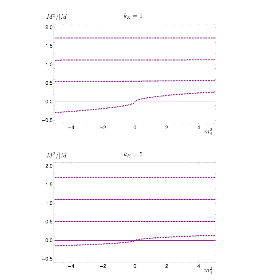
Figure 2: Mass spectrum, $\frac{M^{2}}{|M|}$, of pseudoscalar fluctuations, $\mathfrak{p}^{\hat{\mathcal{A}}}$ (lines) and $\mathfrak{p}^{4}$ (crosses), as a function of the parameter $m_{4}^{2}$, for two representative choices, $k_{\mathcal{X}}=1$ (top panel) and $k_{\mathcal{X}}=5$ (bottom panel). The spectrum shown is that of the theory prior to gauging the $SO(4)$ subgroup, hence the $\mathfrak{p}^{\hat{\mathcal{A}}}$ sector contains massless modes, higgsed away in the gauged case. All plots have $\Delta=2$, $g=5$, $\phi_{I}=\phi_{I}(c)\approx 0.3882$, and the values of the IR and UV cutoffs are, respectively, $\rho_{1}-\rho_{o}=10^{-9}$ and $\rho_{2}-\rho_{o}=5$.

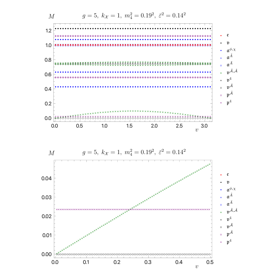
Figure 3: Mass spectrum, $M$, of fluctuations, including pseudoscalar, $\mathfrak{p}^{4}$ (purple crosses), $\mathfrak{p}^{\hat{\mathcal{A}}}$ (purple diamonds), vectors $\mathfrak{v}^{\bar{\mathcal{A}}}$ (black diamonds), $\mathfrak{v}^{4}$ (black crosses), $\mathfrak{v}^{\hat{\mathcal{A}}}$ and $\mathfrak{v}^{\tilde{\mathcal{A}}}$ (green crosses), scalars $\mathfrak{a}^{\bar{A}}$ (blue diamond), and $\mathfrak{a}^{\hat{A}}$ (blue crosses), active scalars, $\mathfrak{a}^{\phi},\mathfrak{a}^{\chi}$ (blue dots), graviphoton $\mathfrak{v}$ (black dots), and spin-2 tensors, $\mathfrak{e}$ (red dots), as a function of the misalignement angle, $v$, for fixed values of $k_{\mathcal{X}},m_{4}^{2}$, and $\bar{\varepsilon}$. The bottom panel is a detail of the top one. All plots have $\Delta=2$, $g=5$, and $\phi_{I}=\phi_{I}(c)\approx 0.3882$, and the values of the IR and UV cutoffs are, respectively, given by $\rho_{1}-\rho_{o}=10^{-9}$ and $\rho_{2}-\rho_{o}=5$.

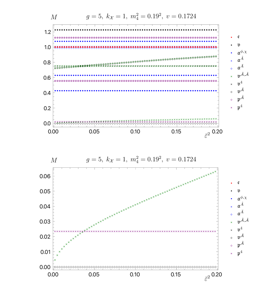
Figure 4: Mass spectrum, $M$, of fluctuations, including pseudoscalar, $\mathfrak{p}^{4}$ (purple crosses), $\mathfrak{p}^{\hat{\mathcal{A}}}$ (purple diamonds), vectors $\mathfrak{v}^{\bar{\mathcal{A}}}$ (black diamonds), $\mathfrak{v}^{4}$ (black crosses), $\mathfrak{v}^{\hat{\mathcal{A}}}$ and $\mathfrak{v}^{\tilde{\mathcal{A}}}$ (green crosses), scalars $\mathfrak{a}^{\bar{A}}$ (blue diamond), and $\mathfrak{a}^{\hat{A}}$ (blue crosses), active scalars, $\mathfrak{a}^{\phi},\mathfrak{a}^{\chi}$ (blue dots), graviphoton $\mathfrak{v}$ (black dots), and spin-2 tensors, $\mathfrak{e}$ (red dots), as a function of the parameter $\bar{\varepsilon}^{2}$, for fixed values of $k_{\mathcal{X}},m_{4}^{2}$, and $v$. The bottom panel is a detail of the top one. All plots have $\Delta=2$, $g=5$, $\phi_{I}=\phi_{I}(c)\approx 0.3882$, and the values of the IR and UV cutoffs are, respectively, given by $\rho_{1}-\rho_{o}=10^{-9}$ and $\rho_{2}-\rho_{o}=5$.

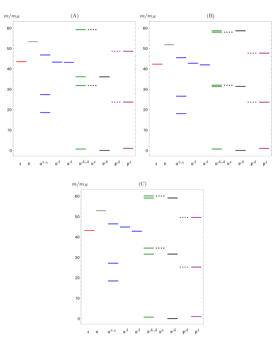
Figure 5: Mass spectrum, $M$, of fluctuations, normalized to the mass, $m_{H}$, of the lightest $\mathfrak{p}^{4}$ state, including pseudoscalars, $\mathfrak{p}^{\hat{\mathcal{A}}}$ (purple), $\mathfrak{p}^{4}$ (purple dashed), vectors, $\mathfrak{v}^{\hat{\mathcal{A}}}$ and $\mathfrak{v}^{\tilde{\mathcal{A}}}$ (green), $\mathfrak{v}^{\bar{\mathcal{A}}}$ (black), $\mathfrak{v}^{4}$ (black dahsed), $v$ (black dotted), scalars, $\mathfrak{a}^{\phi},\mathfrak{a}^{\chi},\mathfrak{a}^{\bar{A}},\mathfrak{a}^{\hat{A}}$ (blue) and spin-2 tensors, $\mathfrak{e}$ (red), for three values of the coupling $g$: (A) $g=2,\;v=0.15,\;g_{4}=0.7,\;m_{4}^{2}=0.185^{2}$, (B) $g=5,\;v=0.1724,\;g_{4}=0.7,\;m_{4}^{2}=0.19^{2}$, (C) $g=8,\;v=0.17,\;g_{4}=0.7,\;m_{4}^{2}=0.185^{2}$. All plots have $\Delta=2$, $\phi_{I}=\phi_{I}(c)\approx 0.3882$, and $k_{\mathcal{X}}=1$. The IR and UV cutoffs are given by $\rho_{1}-\rho_{o}=10^{-9}$ and $\rho_{2}-\rho_{o}=5$, respectively.

In this section, we present examples of the numerical results we obtained for the complete mass spectrum of fluctuations, and its dependence on the model parameters. For concreteness, we set $\Delta=2$, $\phi_{I}=\phi_{I}(c)\approx 0.3882$, $\rho_{2}-\rho_{o}=5$, and $\rho_{1}-\rho_{o}=10^{-9}$, throughout the section. Figures 2–5 illustrate the spectrum dependence on the residual freedom encoded in the choices of $\bar{\varepsilon}$, $g$, $v$, $m_{4}^{2}$, and $k_{\mathcal{X}}$. All spectra, except for Fig. 5, are normalised so that the lightest of the $SO(3)$-singlet spin-2 fluctuations, $\mathfrak{e}_{\mu\nu}$, has unit mass.

Figure 2 displays the dependence of the mass spectrum of the pseudoscalar fluctuations, $\mathfrak{p}^{\hat{\mathcal{A}}}$ and $\mathfrak{p}^{4}$, as a function of the parameter $m_{4}^{2}$, for two representative choices of $k_{\mathcal{X}}$. The spectra in these two sectors do not depend on $\bar{\varepsilon}$ or $v$. Several interesting features are worth commenting about. We notice that the spectrum of $\mathfrak{p}^{\hat{\mathcal{A}}}$ contains three exactly massless states, that disappear when the $SO(4)$ subgroup is gauged, and we work in unitary gauge, as they provide the longitudinal components for three of the vector bosons. A tachyonic mode appears in $\mathfrak{p}^{4}$ if one chooses $m_{4}^{2}<0$, which is hence forbidden. Positive, but small values of $m_{4}^{2}$, close to zero, lead to a small mass for the physical state corresponding to the PNGB responsible for $SO(4)$ spontaneous symmetry breaking. (If this were a composite Higgs model, such a state would be identified with the Higgs boson.)

Figures 3 and 4 show the complete spectra, for representative choices of $g$, $k_{\mathcal{X}}$, $\Delta$, $\phi_{I}$, and $m_{4}^{2}$, as a function of $v$ and $\bar{\varepsilon}^{2}$, respectively. Superficially, the spectra appear to be quite complicated, due to the large number of states, and details depend on the choices of parameters. Yet, the figures display a few important general features. First, only a small number of states are light: the massless vectors corresponding to zero modes in the unbroken, gauged $SO(3)$ sector, the lightest of the $\mathfrak{p}^{4}$ pseudoscalars, and the lightest combination of vectors in the $SO(4)/SO(3)$ coset. All other states have masses that are of the order of the typical scale in the theory, that we identify with the mass of the lightest spin-2 state. A small hierarchy emerges between these two groups of states. Furthermore, as expected on general grounds, the mass of the lightest vector states grows when either of $v$ or $\bar{\varepsilon}^{2}$ is small and growing, and vanishes when either of these two parameters vanishes, which are the natural expectations for vector bosons associated with the Higgs mechanism for spontaneous breaking of a weakly coupled gauge theory.

In Figure 5, we show three numerical examples of the spectrum, aimed at illustrating how a semi-realistic implementation of this model as a CHM would look like. We set aside the differences with the standard model, purely for illustration purposes, and interpret the lightest state in the $\mathfrak{p}^{4}$ fluctuations as the Higgs boson. For the sole purposes of this exercise, we call its mass $m_{H}$, and measure the other masses in units of $m_{H}$. We fix $\Delta=2$ and $\phi_{I}=\phi_{I}(c)\approx 0.3882$, impose the requirement that $g_{4}=\bar{\varepsilon}g=0.7$—of the order of the $SU(2)_{L}$ coupling in the standard model—and adjust the other parameters so that the ratio of mass between the lightest fluctuation in the spin-1 ($v^{\hat{\mathcal{A}}}$ and $v^{\tilde{\mathcal{A}}}$) sector, and the spin-0 ($\mathfrak{p}^{4}$) sector, be approximately given by $M_{Z}/m_{H}\simeq 0.73$—the ratio between the experimental values of the mass of the $Z$ and Higgs bosons.

This model is not realistic, and this final exercise should be taken with a grain of salt. Yet, it meets its purpose, and demonstrates that it is possible, within this model, to produce a small hierarchy between the Higgs and $Z$ mass on one side, and, on the other side, the towers of new bound states predicted by the theory. It is also worth noting that the next-to-lightest states appear to be the spin-0 states, with spin-1 states and spin-2 states significantly heavier.

VII Outlook

In summary, we demonstrated how to build a bottom-up, holographic model that, at low energies, can be interpreted in dual field theory terms as a sigma-model with $SO(5)$ global symmetry broken to $SO(4)$. An $SO(4)$ subgroup is gauged. The presence of explicit $SO(5)$ symmetry-breaking interactions leads to vacuum misalignment and to the spontaneous breaking of the gauged $SO(4)$ to its $SO(3)$ gauge group. Much of this paper is devoted to the non-trivial development of the formalism, showing that symmetry breaking can be consistently triggered by a bulk scalar field in the gravity theory, in which the $SO(5)$ is gauged. It is worth noticing that this can be done without violating the gauge principle, despite the presence of explicit symmetry breaking in the dual field theory. But this can be done consistently only if the bulk field triggering symmetry breaking corresponds in the dual field theory to an operator with scaling dimension restricted to the range $\frac{D-3}{2}\leq\Delta\leq\frac{D+1}{2}$, for reasons described in the body of the paper.

A significant distinctive feature of this proposal is that the gravity background is completely smooth, in a way that mimics confinement in the dual field theory and leads to the introduction of a mass gap. Although more sophisticated holographic descriptions of confinement may require further extensions, and although we did not yet implement a realistic realisation of the electroweak model, the study of the spectrum we performed and reported here indicates that the phenomenology is quite simple, as expected in CHMs based on the $SO(5)/SO(4)$ coset. All the new particles are parametrically heavy in respect to the bosons that play the role of the $Z$, $W$, and Higgs boson. Because a (custodial) $SO(4)$ symmetry is built into the model, one expects a realistic realisation of a CHM based on this model to have escaped indirect detection although a detailed calculation of all precision on electroweak parameters is needed.

To build a fully realistic model, that might be detectable in direct collider searches, requires additional non-trivial steps. First, the model has a gauged $SO(4)$ symmetry, while the SM gauge symmetry is $SU(2)_{L}\times U(1)_{Y}$, and, furthermore, the quantum assignments of the standard-model fermions require identifying an additional $U(1)$ global symmetry, related to baryon and lepton number, so that hypercharge assignments are realistic. We leave this task for future work.

Second, this theory does not contain fermions. We anticipated in the body of the paper that we could proceed in two ways towards their introduction: either by assuming that all fermions are localised on the UV boundary, or that there are additional bulk fermions, transforming in the spinorial representation, $4$, of $SO(5)$. These ingredients would then determine the mechanism for mass generation for the SM fermions, and in turn the contribution of the fermions to the effective potential triggering spontaneous symmetry breaking of the gauge symmetry via vacuum misalignment. Also this task is left for future investigations.

Finally, the techniques illustrated in this paper can be applied to a large class of holographic models in which bulk scalar fields implement symmetry breaking. In particular, there are clear similarities between the gravity set up we discussed here and the one in Ref. Elander:2021kxk , which is based on maximal supergravity in $D=7$ dimensions, and has bulk $SO(5)$ gauge symmetry. As discussed in the Introduction, it is still an open challenge to identify a UV-complete CHM model based on the $SO(5)/SO(4)$ coset, in which the gravity theory is embedded into a known supergravity. The results of this paper provide a major step in this direction.

Appendix A Basis of $SO(5)$ generators

We present here an example of a basis of $SO(5)$ generators, used in the body of the paper, taken from Ref. Elander:2023aow .

$$t^{1} = \frac{i}{2}\left(\begin{array}[]{ccccc}0&0&0&0&-1\\ 0&0&0&0&0\\ 0&0&0&0&0\\ 0&0&0&0&0\\ 1&0&0&0&0\end{array}\right)\,,\quad t^{2}=\frac{i}{2}\left(\begin{array}[]{ccccc}0&0&0&0&0\\ 0&0&0&0&-1\\ 0&0&0&0&0\\ 0&0&0&0&0\\ 0&1&0&0&0\end{array}\right)\,,\quad t^{3}=\frac{i}{2}\left(\begin{array}[]{ccccc}0&0&0&0&0\\ 0&0&0&0&0\\ 0&0&0&0&-1\\ 0&0&0&0&0\\ 0&0&1&0&0\end{array}\right)\,,\quad t^{4}=\frac{i}{2}\left(\begin{array}[]{ccccc}0&0&0&0&0\\ 0&0&0&0&0\\ 0&0&0&0&0\\ 0&0&0&0&-1\\ 0&0&0&1&0\end{array}\right)\,,$$ (198)

$$t^{5} = \frac{i}{2}\left(\begin{array}[]{ccccc}0&0&0&-1&0\\ 0&0&0&0&0\\ 0&0&0&0&0\\ 1&0&0&0&0\\ 0&0&0&0&0\end{array}\right)\,,\quad t^{6}=\frac{i}{2}\left(\begin{array}[]{ccccc}0&0&0&0&0\\ 0&0&0&-1&0\\ 0&0&0&0&0\\ 0&1&0&0&0\\ 0&0&0&0&0\end{array}\right)\,,\quad t^{7}=\frac{i}{2}\left(\begin{array}[]{ccccc}0&0&0&0&0\\ 0&0&0&0&0\\ 0&0&0&-1&0\\ 0&0&1&0&0\\ 0&0&0&0&0\end{array}\right)\,,$$ (214)

$$t^{8} = \frac{i}{2}\left(\begin{array}[]{ccccc}0&0&-1&0&0\\ 0&0&0&0&0\\ 1&0&0&0&0\\ 0&0&0&0&0\\ 0&0&0&0&0\end{array}\right)\,,\quad t^{9}=\frac{i}{2}\left(\begin{array}[]{ccccc}0&0&0&0&0\\ 0&0&-1&0&0\\ 0&1&0&0&0\\ 0&0&0&0&0\\ 0&0&0&0&0\end{array}\right)\,,\quad t^{10}=\frac{i}{2}\left(\begin{array}[]{ccccc}0&-1&0&0&0\\ 1&0&0&0&0\\ 0&0&0&0&0\\ 0&0&0&0&0\\ 0&0&0&0&0\end{array}\right)\,,\quad$$ (230)

We find it convenient to present also a basis of $SU(4)$, adapted from Ref. Bennett:2017kga , written in terms of $4\times 4$ Hermitian matrices. The adjoint representation of $SU(4)$ decomposes as $15=5\oplus 10$ in $Sp(4)\sim SO(5)$, both being used in the body of the paper. We order the basis so that $\Gamma^{A}$, for $A=1,\,\cdots,\,5$, spans the coset $SU(4)/Sp(4)$, and hence can be used to describe the $5$ of $Sp(4)$, while the generators of $Sp(4)$ are denoted $T^{A}$, with $A=1,\,\cdots,\,10$. We conventionally normalise ${\rm Tr}\,(T^{A}T^{B})=\frac{1}{4}\delta^{AB}={\rm Tr}\,(\Gamma^{A}\Gamma^{B})$, for all the $SU(4)$ matrices. The $\Gamma^{A}$ matrices are

$$\Gamma^{1} = \frac{1}{4}\left(\begin{array}[]{cccc}0&1&0&0\cr 1&0&0&0\cr 0&0&0&1\cr 0&0&1&0\end{array}\right)\,,\qquad\Gamma^{2}\,=\,\frac{1}{4}\left(\begin{array}[]{cccc}0&-i&0&0\cr i&0&0&0\cr 0&0&0&i\cr 0&0&-i&0\end{array}\right)\,,\qquad\Gamma^{3}\,=\,\frac{1}{4}\left(\begin{array}[]{cccc}0&0&0&-i\cr 0&0&i&0\cr 0&-i&0&0\cr i&0&0&0\end{array}\right)\,,$$ (243)

$$\Gamma^{4} = \frac{1}{4}\left(\begin{array}[]{cccc}0&0&0&1\cr 0&0&-1&0\cr 0&-1&0&0\cr 1&0&0&0\end{array}\right)\,,\qquad\Gamma^{5}\,=\,\frac{1}{4}\left(\begin{array}[]{cccc}1&0&0&0\cr 0&-1&0&0\cr 0&0&1&0\cr 0&0&0&-1\end{array}\right)\,.$$ (252)

The generators of $Sp(4)$, the $10$ of $Sp(4)\sim SO(5)$ are:

$$T^{1} = \frac{1}{4}\left(\begin{array}[]{cccc}0&i&0&0\cr-i&0&0&0\cr 0&0&0&i\cr 0&0&-i&0\end{array}\right)\,,\qquad T^{2}\,=\,\frac{1}{4}\left(\begin{array}[]{cccc}0&1&0&0\cr 1&0&0&0\cr 0&0&0&-1\cr 0&0&-1&0\end{array}\right)\,,\qquad T^{3}\,=\,\frac{1}{4}\left(\begin{array}[]{cccc}0&0&0&1\cr 0&0&1&0\cr 0&1&0&0\cr 1&0&0&0\end{array}\right)\,,$$ (265)

$$T^{4} = \frac{1}{4}\left(\begin{array}[]{cccc}0&0&0&i\cr 0&0&i&0\cr 0&-i&0&0\cr-i&0&0&0\end{array}\right)\,,\qquad T^{5}\,=\,\frac{1}{4}\left(\begin{array}[]{cccc}0&0&i&0\cr 0&0&0&-i\cr-i&0&0&0\cr 0&i&0&0\end{array}\right)\,,\qquad T^{6}\,=\,\frac{1}{4}\left(\begin{array}[]{cccc}0&0&1&0\cr 0&0&0&1\cr 1&0&0&0\cr 0&1&0&0\end{array}\right)\,,$$ (278)

$$T^{7} = \frac{1}{4}\left(\begin{array}[]{cccc}-1&0&0&0\cr 0&-1&0&0\cr 0&0&1&0\cr 0&0&0&1\end{array}\right)\,,\qquad T^{8}\,=\,\frac{1}{4}\left(\begin{array}[]{cccc}0&0&1&0\cr 0&0&0&-1\cr 1&0&0&0\cr 0&-1&0&0\end{array}\right)\,\qquad T^{9}\,=\,\frac{1}{4}\left(\begin{array}[]{cccc}0&0&-i&0\cr 0&0&0&-i\cr i&0&0&0\cr 0&i&0&0\end{array}\right)\,$$ (291)

$$T^{10} = \frac{1}{4}\left(\begin{array}[]{cccc}1&0&0&0\cr 0&-1&0&0\cr 0&0&-1&0\cr 0&0&0&1\end{array}\right)\,.$$ (296)

They can be written as commutators of two $\Gamma^{A}$ matrices. For example, $T^{1}=-2i\left[\Gamma^{1},\,\Gamma^{5}\right]$. Similar relations hold for the other generators.

Appendix B Five-dimensional formalism

In this Appendix, we report technical details on the treatment of gauge-invariant fluctuations. Most of this material is borrowed from the literature, but we find it useful to summarise it here, to make the exposition self-contained, and the notation coherent and self-consistent.

B.1 Scalars coupled to gravity

We report here the salient features of the gauge-invariant formalism developed in Refs. Bianchi:2003ug ; Berg:2005pd ; Berg:2006xy ; Elander:2009bm ; Elander:2010wd ; Elander:2014ola ; Elander:2017cle ; Elander:2017hyr . Borrowing from Refs. Berg:2005pd ; Elander:2010wd , consider $n$ real scalars, $\Phi^{a}$, with $a=1\,,\,\cdots\,,\,n$; the action, ${\cal S}_{D}$, is written in general as follows:

$${\cal S}_{D} = \int\mbox{d}^{D}x\sqrt{-g}\left[\frac{{R}}{4}-\frac{1}{2}G_{ab}g^{MN}\partial_{M}\Phi^{a}\partial_{N}\Phi^{b}-{\mathcal{V}}(\Phi^{a})\right]\,.$$ (297)

(In this paper, the relevant scalars are denoted as $\{\chi,\phi,{\cal B}_{6}^{\tilde{\cal A}},{\cal A}_{6}^{\bar{\cal A}},{\cal B}_{6}^{\hat{\cal A}},{\cal A}_{6}^{4}\}$, hence $n=12$, and the dimensionality of the system is $D=5$.) The backgrounds are described by the ansatz

$$\mbox{d}s^{2}_{D} = \mbox{d}r^{2}+e^{2{A}(r)}\,\eta_{\mu\nu}\mbox{d}x^{\mu}\mbox{d}x^{\nu}\,,$$ (298)

$$\Phi^{a} = \Phi^{a}(r)\,,$$ (299)

in which the background functions depend only on the radial direction, $r$. The connection symbols are

$$\Gamma^{P}_{\,\,\,\,MN} \equiv \frac{1}{2}g^{PQ}\left(\frac{}{}\partial_{M}g_{NQ}+\partial_{N}g_{QM}-\partial_{Q}g_{MN}\right)\,,$$ (300)

while the Riemann tensor is

$$R_{MNP}^{\,\,\,\,\,\,\,\,\,\,\,\,\,\,\,\,\,Q} \equiv \partial_{N}\Gamma^{Q}_{\,\,\,\,MP}-\partial_{M}\Gamma^{Q}_{\,\,\,\,NP}+\Gamma^{S}_{\,\,\,\,MP}\Gamma^{Q}_{\,\,\,\,SN}-\Gamma^{S}_{\,\,\,\,NP}\Gamma^{Q}_{\,\,\,\,SM}\,,$$ (301)

the Ricci tensor is

$$R_{MN} \equiv R_{MPN}^{\,\,\,\,\,\,\,\,\,\,\,\,\,\,\,\,\,P}\,,$$ (302)

and the Ricci scalar is

$${R} \equiv R_{MN}g^{MN}\,.$$ (303)

The conventions are such that the (gravity) covariant derivative for a $(1,1)$-tensor takes the form

$$\nabla_{M}T^{P}_{\,\,\,\,N} \equiv \partial_{M}T^{P}_{\,\,\,\,N}+\Gamma^{P}_{\,\,\,\,MQ}T^{Q}_{\,\,\,\,N}-\Gamma^{Q}_{\,\,\,\,MN}T^{P}_{\,\,\,\,Q}\,,$$ (304)

and generalises to any $(m,n)$-tensors.

Because of the presence of boundaries, at which the five-dimensional manifold ends on two four-dimensional manifolds, one must introduce the induced metric, $\tilde{g}_{MN}$, for which we adopt the following conventions:

$$\tilde{g}_{MN} \equiv g_{MN}-N_{M}N_{M}\,,$$ (305)

where $N_{M}$ is the ortho-normalised vector to the boundary, which satisfies the defining properties:

$$g_{MN}N^{M}N^{N} = 1\,,\qquad{\rm and}\qquad\tilde{g}_{MN}N^{N}\,=\,0\,.$$ (306)

It is conventional to orient the ortho-normalised vector so that it points outside of the space. Yet, in the body of the paper, we use a definition of $N_{M}$ which aligns it along the holographic direction, so that it points outwards from the boundary at the UV, but inside the space at the IR boundary. For this reason, different signs appear in front of the terms localised at the two boundaries in Eq. (108). The extrinsic curvature, $K$, is given by $K\equiv\tilde{g}^{MN}K_{MN}$, in terms of the symmetric tensor

$$K_{MN} \equiv \nabla_{M}N_{N}\,=\,\partial_{M}N_{N}-\Gamma^{Q}_{\,\,\,\,MN}N_{Q}\,.$$ (307)

In parallel to the space-time, in the internal space, the sigma-model connection descends from the sigma-model metric, $G_{ab}$, and the sigma-model derivative, $\partial_{b}=\frac{\partial}{\partial\Phi^{b}}$, to read

$${\cal G}^{d}_{\,\,\,\,ab} \equiv \frac{1}{2}G^{dc}\left(\frac{}{}\partial_{a}G_{cb}+\partial_{b}G_{ca}-\partial_{c}G_{ab}\right)\,.$$ (308)

The sigma-model Riemann tensor is

$${\cal R}^{a}_{\,\,\,\,bcd} \equiv \partial_{c}{\cal G}^{a}_{\,\,\,\,bd}-\partial_{d}{\cal G}^{a}_{\,\,\,\,bc}+{\cal G}^{e}_{\,\,\,\,bd}{\cal G}^{a}_{\,\,\,\,ce}-{\cal G}^{e}_{\,\,\,\,bc}{\cal G}^{a}_{\,\,\,\,de}\,,$$ (309)

while the sigma-model covariant derivative is

$$D_{b}X^{d}_{\,\,\,\,a} \equiv \partial_{b}X^{d}_{\,\,\,\,a}+{\cal G}^{d}_{\,\,\,\,cb}X^{c}_{\,\,\,\,a}-{\cal G}^{c}_{\,\,\,\,ab}X^{d}_{\,\,\,\,c}\,.$$ (310)

The equations of motion, satisfied by the background scalars, are the following:

$$\partial_{r}^{2}\Phi^{a}\,+\,(D-1)\partial_{r}{A}\partial_{r}\Phi^{a}\,+\,{\cal G}^{a}_{\,\,\,\,bc}\partial_{r}\Phi^{b}\partial_{r}\Phi^{c}\,-\,\mathcal{V}^{a} = 0\,,$$ (311)

where the sigma-model derivatives are given by $\mathcal{V}^{a}\equiv G^{ab}\partial_{b}\mathcal{V}$, and $\partial_{b}\mathcal{V}\equiv\frac{\partial\mathcal{V}}{\partial\Phi^{b}}$. The Einstein equations reduce to

$$(D-1)(\partial_{r}{A})^{2}\,+\,\partial_{r}^{2}{A}\,+\,\frac{4}{D-2}\mathcal{V} = 0\,,$$ (312)

$$(D-1)(D-2)(\partial_{r}{A})^{2}\,-\,2G_{ab}\partial_{r}\Phi^{a}\partial_{r}\Phi^{b}\,+\,4\mathcal{V} = 0\,.$$ (313)

B.1.1 Tensor and scalar fluctuations

Following Refs. Bianchi:2003ug ; Berg:2006xy ; Berg:2005pd ; Elander:2009bm ; Elander:2010wd , the scalar fields can be written as

$$\Phi^{a}(x^{\mu},r)=\Phi^{a}(r)+\varphi^{a}(x^{\mu},r)\,,$$ (314)

where $\varphi^{a}(x^{\mu},r)$ are small fluctuations around the background solutions, $\Phi^{a}(r)$. The metric fluctuations are decomposed with the ADM formalism Arnowitt:1962hi :

$$\mbox{d}s_{D}^{2} = \left((1+\nu)^{2}+\nu_{\sigma}\nu^{\sigma}\right)\mbox{d}r^{2}+2\nu_{\mu}\mbox{d}x^{\mu}\mbox{d}r+e^{2{A}(r)}\left(\eta_{\mu\nu}+h_{\mu\nu}\right)\mbox{d}x^{\mu}\mbox{d}x^{\nu}\,,$$ (315)

where

$$h^{\mu}{}_{\nu} = \mathfrak{e}^{\mu}{}_{\nu}+iq^{\mu}\epsilon_{\nu}+iq_{\nu}\epsilon^{\mu}+\frac{q^{\mu}q_{\nu}}{q^{2}}H+\frac{1}{D-2}\delta^{\mu}{}_{\nu}h.$$ (316)

Here, $\nu(x^{\mu},r)$, $\nu^{\mu}(x^{\mu},r)$, $\mathfrak{e}^{\mu}{}_{\nu}(x^{\mu},r)$, $\epsilon^{\mu}(x^{\mu},r)$, $H(x^{\mu},r)$, and $h(x^{\mu},r)$ are small fluctuations around the background metric, of which $\mathfrak{e}^{\mu}{}_{\nu}$ is transverse and traceless (while $\epsilon^{\mu}$ is transverse), and gauge invariant.

The other (diffeomorphism) gauge-invariant combinations are

$$\mathfrak{a}^{a} = \varphi^{a}-\frac{\partial_{r}\Phi^{a}}{2(D-2)\partial_{r}{A}}h\,,$$ (317)

$$\mathfrak{b} = \nu-\partial_{r}\left(\frac{h}{2(D-2)\partial_{r}{A}}\right)\,,$$ (318)

$$\mathfrak{c} = e^{-2{A}}\partial_{\mu}\nu^{\mu}-\frac{e^{-2{A}}q^{2}h}{2(D-2)\partial_{r}A}-\frac{1}{2}\partial_{r}H\,,$$ (319)

$$\mathfrak{d}^{\mu} = e^{-2{A}}P^{\mu}{}_{\nu}\nu^{\nu}-\partial_{r}\epsilon^{\mu}\,.$$ (320)

The algebraic nature of the equations for $\mathfrak{b}$ and $\mathfrak{c}$ allows us to decouple the equations and solve them.

The tensor fluctuations $\mathfrak{e}^{\mu}{}_{\nu}$ obey the equation of motion

$$\left[\partial_{r}^{2}+(D-1)\partial_{r}{A}\partial_{r}-e^{-2{A}(r)}q^{2}\right]\mathfrak{e}^{\mu}_{\,\,\,\nu}=0\,,$$ (321)

with boundary conditions given by

$$\left.\frac{}{}\partial_{r}\mathfrak{e}^{\mu}_{\,\,\,\nu}\right|_{r=r_{i}}=0\,.$$ (322)

The equation of motion for $\mathfrak{d}^{\mu}$ is algebraic and does not lead to a spectrum of states. The equations of motion for $\mathfrak{a}^{a}$ obey the following equations of motion:

$$0 = \Big{[}{\cal D}_{r}^{2}+(D-1)\partial_{r}{A}{\cal D}_{r}-e^{-2{A}}q^{2}\Big{]}\mathfrak{a}^{a}\,\,$$

$$-\Big{[}{\mathcal{V}}^{\,\,a}{}_{\,|c}-\mathcal{R}^{a}{}_{bcd}\partial_{r}\Phi^{b}\partial_{r}\Phi^{d}+\frac{4(\partial_{r}\Phi^{a}{\mathcal{V}}^{\,b}+{\mathcal{V}}^{\,a}\partial_{r}\Phi^{b})G_{bc}}{(D-2)\partial_{r}{A}}+\frac{16{\mathcal{V}}\partial_{r}\Phi^{a}\partial_{r}\Phi^{b}G_{bc}}{(D-2)^{2}(\partial_{r}{A})^{2}}\Big{]}\mathfrak{a}^{c}\,,$$

while the boundary conditions are given by

$$\frac{2e^{2A}\partial_{r}\Phi^{a}}{(D-2)q^{2}\partial_{r}{A}}\left[\partial_{r}\Phi^{b}{\cal D}_{r}-\frac{4{\cal V}\partial_{r}\Phi^{b}}{(D-2)\partial_{r}{A}}-{\cal V}^{b}\right]\mathfrak{a}_{b}-\mathfrak{a}^{a}\Big{|}_{r_{i}}=0\,.$$ (324)

The background covariant derivative is $\mathcal{D}_{r}\mathfrak{a}^{a}\equiv\partial_{r}\mathfrak{a}^{a}+\mathcal{G}^{a}_{\ bc}\partial_{r}\Phi^{b}\mathfrak{a}^{c}$, and ${\mathcal{V}}^{a}{}_{|b}\equiv\frac{\partial{\mathcal{V}}^{a}}{\partial\Phi^{b}}+\mathcal{G}^{a}_{\ bc}{\mathcal{V}}^{c}$.

B.2 Vectors, pseudoscalars, and spurions

In this appendix, we provide the gauge fixing terms and equations of motion for the spin-1 and spin-0 fluctuations introduced in Sect. IV. The resulting equations for the fields defined in Eq. (130) (except for $\chi_{M}$) and other fields interacting with them are distributed in the following subsections. Section  B.2.1 reports the equations of motion and boundary conditions for $\mathcal{B}_{M}{}^{\tilde{\mathcal{A}}}$ and $\mathcal{B}_{M}{}^{\hat{\mathcal{A}}}$, and for the associated spin-0 states. Section B.2.2 discusses $\mathcal{A}_{M}{}^{4}$ and Sect. B.2.3 focuses on $\mathcal{A}_{M}{}^{\bar{\mathcal{A}}}$, respectively.

B.2.1 The $\mathcal{B}_{M}{}^{\hat{\mathcal{A}}}$ and $\mathcal{B}_{M}{}^{\tilde{\mathcal{A}}}$ sectors

Following the procedure in Ref. Elander:2018aub , we choose the gauge fixing terms for $\mathcal{B}_{M}{}^{\hat{\mathcal{A}}}$ and $\mathcal{B}_{M}{}^{\tilde{\mathcal{A}}}$ to be

$$\mathcal{S}_{\hat{\xi}}^{(1)} = \int\mathrm{d}^{4}q\mathrm{~{}d}r\left\{-\frac{H^{(1)}_{\hat{\mathcal{A}}\hat{\mathcal{A}}}}{2\hat{\xi}}\left[iq^{\mu}\mathcal{B}_{\mu}{}^{\hat{\mathcal{A}}}(-q)-\frac{g\sin(v)}{2v}\frac{\hat{\xi}}{H^{(1)}_{\hat{\mathcal{A}}\hat{\mathcal{A}}}}G^{(1)}_{\hat{\mathcal{A}}\hat{\mathcal{A}}}e^{2A}\pi^{\hat{\mathcal{A}}}(-q)-\frac{\hat{\xi}}{H^{(1)}_{\hat{\mathcal{A}}\hat{\mathcal{A}}}}\partial_{r}\left(H^{(1)}_{\hat{\mathcal{A}}\hat{\mathcal{A}}}e^{2A}\mathcal{B}_{5}{}^{\hat{\mathcal{A}}}(-q)\right)\right]\times\right.$$ (325)

$$\times{\left.\left[-iq^{\nu}\mathcal{B}_{\nu}{}^{\hat{\mathcal{A}}}(q)-\frac{g\sin(v)}{2v}\frac{\hat{\xi}}{H^{(1)}_{\hat{\mathcal{A}}\hat{\mathcal{A}}}}G^{(1)}_{\hat{\mathcal{A}}\hat{\mathcal{A}}}e^{2A}\pi^{\hat{\mathcal{A}}}(q)-\frac{\hat{\xi}}{H^{(1)}_{\hat{\mathcal{A}}\hat{\mathcal{A}}}}\partial_{r}\left(H^{(1)}_{\hat{\mathcal{A}}\hat{\mathcal{A}}}e^{2A}\mathcal{B}_{5}{}^{\hat{\mathcal{A}}}(q)\right)\right]\right\}\,,}$$

and

$$\mathcal{S}_{\tilde{\xi}}^{(1)} = \int\mathrm{d}^{4}q\mathrm{~{}d}r\left\{-\frac{H^{(1)}_{\tilde{\mathcal{A}}\tilde{\mathcal{A}}}}{2\tilde{\xi}}\left[iq^{\mu}\mathcal{B}_{\mu}{}^{\tilde{\mathcal{A}}}(-q)-\frac{\tilde{\xi}}{H^{(1)}_{\tilde{\mathcal{A}}\tilde{\mathcal{A}}}}\partial_{r}\left(H^{(1)}_{\tilde{\mathcal{A}}\tilde{\mathcal{A}}}e^{2A}\mathcal{B}_{5}{}^{\tilde{\mathcal{A}}}(-q)\right)\right]\times\right.$$ (326)

$$\times{\left.\left[-iq^{\nu}\mathcal{B}_{\nu}{}^{\tilde{\mathcal{A}}}(q)-\frac{\tilde{\xi}}{H^{(1)}_{\tilde{\mathcal{A}}\tilde{\mathcal{A}}}}\partial_{r}\left(H^{(1)}_{\tilde{\mathcal{A}}\tilde{\mathcal{A}}}e^{2A}\mathcal{B}_{5}{}^{\tilde{\mathcal{A}}}(q)\right)\right]\right\}\,,}$$

where $\hat{\xi}$ and $\tilde{\xi}$ are gauge-fixing parameters. The boundary-localised gauge fixing terms at $r=r_{2}$ are

$$\mathcal{S}_{\hat{M}}^{(1)}= \int\mathrm{d}^{4}q\mathrm{~{}d}r\delta\left(r-r_{2}\right)\left\{-\frac{1}{2\hat{M}_{2}}\left[iq^{\mu}\mathcal{B}_{\mu}{}^{\hat{\mathcal{A}}}(-q)+\hat{M}_{2}H^{(1)}_{\hat{\mathcal{A}}\hat{\mathcal{A}}}e^{2A}\mathcal{B}_{5}{}^{\hat{\mathcal{A}}}(-q)-\hat{M}_{2}K_{5}\frac{gv_{5}}{2}e^{2A}\cos(v)P^{\hat{\mathcal{A}}}_{5}(-q)\right.\right.$$ (327)

$$\left.\left.-\frac{g\sin(v)}{2v}\hat{M}_{2}C_{2\,\hat{\mathcal{A}}\hat{\mathcal{A}}}^{(1)}e^{2A}\pi^{\hat{\mathcal{A}}}(-q)\right]\times\left[(q\rightarrow-q)\right]\right\}\,,$$

and

$$\mathcal{S}_{\tilde{M}}^{(1)}= \int\mathrm{d}^{4}q\mathrm{~{}d}r\delta\left(r-r_{2}\right)\left\{-\frac{1}{2\tilde{M}_{2}}\left[iq^{\mu}\mathcal{B}_{\mu}{}^{\tilde{\mathcal{A}}}(-q)+\tilde{M}_{2}H^{(1)}_{\tilde{\mathcal{A}}\tilde{\mathcal{A}}}e^{2A}\mathcal{B}_{5}{}^{\tilde{\mathcal{A}}}(-q)+\tilde{M}_{2}K_{5}\frac{gv_{5}}{2}e^{2A}\sin(v)P^{\hat{\mathcal{A}}}_{5}(-q)\right]\right.\times$$ (328)

$$\left.\times\left[(q\rightarrow-q)\right]\right\}\,.$$

The boundary-localised gauge fixing parameters, $\hat{M}_{2}$ and $\tilde{M}_{2}$, are independent of the bulk dynamics. Gauge fixing at $r=r_{1}$ can be done in a similar manner. Gathering terms from the action Eq. (123) and gauge fixing terms in Eqs. (325), (326), (327), and (328), the equations of motion and boundary conditions for $\mathcal{B}_{\mu}{}^{\hat{\mathcal{A}}}$ and $\mathcal{B}_{\mu}{}^{\tilde{\mathcal{A}}}$ read

$$0= {\left[q^{2}H^{(1)}_{\hat{\mathcal{A}}\hat{\mathcal{A}}}-\partial_{r}\left(H^{(1)}_{\hat{\mathcal{A}}\hat{\mathcal{A}}}e^{2A}\partial_{r}\right)+\left(\frac{g}{2}\right)^{2}G^{(1)}_{\hat{\mathcal{A}}\hat{\mathcal{A}}}e^{2A}\right]P^{\mu\nu}\mathcal{B}_{\mu}{}^{\hat{\mathcal{A}}}(q,r)},$$ (329)

$$0= {\left.\left[q^{2}D_{2\,\hat{\mathcal{A}}\hat{\mathcal{A}}}^{(1)}+H^{(1)}_{\hat{\mathcal{A}}\hat{\mathcal{A}}}e^{2A}\partial_{r}+e^{2A}\left(\frac{g}{2}\right)^{2}C_{2\,\hat{\mathcal{A}}\hat{\mathcal{A}}}^{(1)}+e^{2A}(\frac{gv_{5}}{2})^{2}K_{5}\cos(v)^{2}\right]P^{\mu\nu}\mathcal{B}_{\nu}{}^{\hat{\mathcal{A}}}(q,r)\right|_{r=r_{2}}}$$

$$+\left.\left[q^{2}D_{2\,\hat{\mathcal{A}}\tilde{\mathcal{A}}}^{(1)}-e^{2A}(\frac{gv_{5}}{2})^{2}K_{5}\cos(v)\sin(v)\right]P^{\mu\nu}\mathcal{B}_{\nu}{}^{\tilde{\mathcal{A}}}(q,r)\right|_{r=r_{2}}\,,$$ (330)

$$0= {\left[\frac{q^{2}}{\hat{\xi}}H^{(1)}_{\hat{\mathcal{A}}\hat{\mathcal{A}}}-\partial_{r}\left(H^{(1)}_{\hat{\mathcal{A}}\hat{\mathcal{A}}}e^{2A}\partial_{r}\right)+\left(\frac{g}{2}\right)^{2}G^{(1)}_{\hat{\mathcal{A}}\hat{\mathcal{A}}}e^{2A}\right]\frac{q^{\mu}q^{\nu}}{q^{2}}\mathcal{B}_{\mu}{}^{\hat{\mathcal{A}}}(q,r)},$$ (331)

$$0= {\left.\left[\frac{q^{2}}{\hat{M}_{2}}+H^{(1)}_{\hat{\mathcal{A}}\hat{\mathcal{A}}}e^{2A}\partial_{r}+e^{2A}\left(\frac{g}{2}\right)^{2}C_{2\,\hat{\mathcal{A}}\hat{\mathcal{A}}}^{(1)}+e^{2A}(\frac{gv_{5}}{2})^{2}K_{5}\cos(v)^{2}\right]\frac{q^{\mu}q^{\nu}}{q^{2}}\mathcal{B}_{\nu}{}^{\hat{\mathcal{A}}}(q,r)\right|_{r=r_{2}}}$$

$${\left.-\left[e^{2A}(\frac{gv_{5}}{2})^{2}K_{5}\cos(v)\sin(v)\right]\frac{q^{\mu}q^{\nu}}{q^{2}}\mathcal{B}_{\nu}{}^{\tilde{\mathcal{A}}}(q,r)\right|_{r=r_{2}}}\,,$$ (332)

$$0= {\left[q^{2}H^{(1)}_{\tilde{\mathcal{A}}\tilde{\mathcal{A}}}-\partial_{r}\left(H^{(1)}_{\tilde{\mathcal{A}}\tilde{\mathcal{A}}}e^{2A}\partial_{r}\right)\right]P^{\mu\nu}\mathcal{B}_{\mu}{}^{\tilde{\mathcal{A}}}(q,r)}\,,$$ (333)

$$0= {\left.\left[q^{2}D_{2\,\tilde{\mathcal{A}}\tilde{\mathcal{A}}}^{(1)}+H^{(1)}_{\tilde{\mathcal{A}}\tilde{\mathcal{A}}}e^{2A}\partial_{r}+e^{2A}(\frac{gv_{5}}{2})^{2}K_{5}\sin(v)^{2}\right]P^{\mu\nu}\mathcal{B}_{\nu}{}^{\tilde{\mathcal{A}}}(q,r)\right|_{r=r_{2}}}$$

$${\left.+\left[q^{2}D_{2\,\tilde{\mathcal{A}}\hat{\mathcal{A}}}^{(1)}-e^{2A}(\frac{gv_{5}}{2})^{2}K_{5}\cos(v)\sin(v)\right]P^{\mu\nu}\mathcal{B}_{\nu}{}^{\hat{\mathcal{A}}}(q,r)\right|_{r=r_{2}}}\,,$$ (334)

$$0= {\left[\frac{q^{2}}{\tilde{\xi}}H^{(1)}_{\tilde{\mathcal{A}}\tilde{\mathcal{A}}}-\partial_{r}\left(H^{(1)}_{\tilde{\mathcal{A}}\tilde{\mathcal{A}}}e^{2A}\partial_{r}\right)\right]\frac{q^{\mu}q^{\nu}}{q^{2}}\mathcal{B}_{\mu}{}^{\tilde{\mathcal{A}}}(q,r)}\,,$$ (335)

$$0= {\left.\left[\frac{q^{2}}{\tilde{M}_{2}}+H^{(1)}_{\tilde{\mathcal{A}}\tilde{\mathcal{A}}}e^{2A}\partial_{r}+e^{2A}(\frac{gv_{5}}{2})^{2}K_{5}\sin(v)^{2}\right]\frac{q^{\mu}q^{\nu}}{q^{2}}\mathcal{B}_{\nu}{}^{\tilde{\mathcal{A}}}(q,r)\right|_{r=r_{2}}}$$

$$-{\left.\left[e^{2A}(\frac{gv_{5}}{2})^{2}K_{5}\cos(v)\sin(v)\right]\frac{q^{\mu}q^{\nu}}{q^{2}}\mathcal{B}_{\nu}{}^{\hat{\mathcal{A}}}(q,r)\right|_{r=r_{2}}}\,.$$ (336)

Equations (329), (331), (333), and (334) can be compared to Eqs. (154), (155), and (157) in the body of the paper.

For pseudoscalar and spurion fields, the equations are obtained from the variation with respect to $\mathcal{B}_{5}{}^{\tilde{\mathcal{A}}}$, $\mathcal{B}_{5}{}^{\hat{\mathcal{A}}}$, $\pi^{\hat{\mathcal{A}}}$ in the bulk and boundary and $P_{5}^{\hat{\mathcal{A}}}$ in the boundary, respectively:

$$0= {\left[q^{2}-\partial_{r}\left(\frac{\tilde{\xi}}{H^{(1)}_{\tilde{\mathcal{A}}\tilde{\mathcal{A}}}}\partial_{r}\left(H^{(1)}_{\tilde{\mathcal{A}}\tilde{\mathcal{A}}}e^{2A}\right)\right)\right]\mathcal{B}_{5}{}^{\tilde{\mathcal{A}}}(q,r)}\,,$$ (337)

$$0= {\left.\left[\tilde{\xi}\frac{e^{-2A}}{H^{(1)}_{\tilde{\mathcal{A}}\tilde{\mathcal{A}}}}\partial_{r}\left(H^{(1)}_{\tilde{\mathcal{A}}\tilde{\mathcal{A}}}e^{2A}\right)+\tilde{M}_{2}H^{(1)}_{\tilde{\mathcal{A}}\tilde{\mathcal{A}}}\right]\mathcal{B}_{5}{}^{\tilde{\mathcal{A}}}(q,r)\right|_{r=r_{2}}+\left.\left[\frac{gv_{5}}{2}\tilde{M}_{2}K_{5}\sin(v)\right]P_{5}^{\hat{\mathcal{A}}}(q)\right|_{r=r_{2}}}\,,$$ (338)

$$0= {\left[q^{2}H^{(1)}_{\hat{\mathcal{A}}\hat{\mathcal{A}}}-H^{(1)}_{\hat{\mathcal{A}}\hat{\mathcal{A}}}\partial_{r}\left(\frac{\hat{\xi}}{H^{(1)}_{\hat{\mathcal{A}}\hat{\mathcal{A}}}}\partial_{r}\left(H^{(1)}_{\hat{\mathcal{A}}\hat{\mathcal{A}}}e^{2A}\right)\right)+\frac{g}{2}^{2}G^{(1)}_{\hat{\mathcal{A}}\hat{\mathcal{A}}}e^{2A}\right]\mathcal{B}_{5}{}^{\hat{\mathcal{A}}}(q,r)}$$

$$+{\frac{g\sin(v)}{2v}\left[G^{(1)}_{\hat{\mathcal{A}}\hat{\mathcal{A}}}e^{2A}\partial_{r}-H^{(1)}_{\hat{\mathcal{A}}\hat{\mathcal{A}}}\partial_{r}\left(\hat{\xi}\frac{G^{(1)}_{\hat{\mathcal{A}}\hat{\mathcal{A}}}e^{2A}}{H^{(1)}_{\hat{\mathcal{A}}\hat{\mathcal{A}}}}\right)\right]\pi^{\hat{\mathcal{A}}}(q,r)}\,,$$ (339)

$$0= {\left.\left[\frac{e^{-2A}}{H^{(1)}_{\tilde{\mathcal{A}}\tilde{\mathcal{A}}}}\partial_{r}\left(\hat{\xi}H^{(1)}_{\hat{\mathcal{A}}\hat{\mathcal{A}}}e^{2A}\right)+\hat{M}_{2}H^{(1)}_{\hat{\mathcal{A}}\hat{\mathcal{A}}}\right]\mathcal{B}_{5}{}^{\hat{\mathcal{A}}}(q,r)-\left[\frac{gv_{5}}{2}\hat{M}_{2}\cos(v)K_{5}\right]P_{5}^{\hat{\mathcal{A}}}(q)\right|_{r=r_{2}}}$$

$$+{\left.\frac{g\sin(v)}{2v}\left[\hat{\xi}\frac{G^{(1)}_{\hat{\mathcal{A}}\hat{\mathcal{A}}}}{H^{(1)}_{\tilde{\mathcal{A}}\tilde{\mathcal{A}}}}-\hat{M}_{2}C_{2\,\hat{\mathcal{A}}\hat{\mathcal{A}}}^{(1)}\right]\pi^{\hat{\mathcal{A}}}(q,r)\right|_{r=r_{2}}}\,,$$ (340)

$$0= {\frac{\sin(v)}{v}\left[\partial_{r}\left(G^{(1)}_{\hat{\mathcal{A}}\hat{\mathcal{A}}}e^{4A}\partial_{r}\right)-G^{(1)}_{\hat{\mathcal{A}}\hat{\mathcal{A}}}e^{2A}q^{2}-\left(\frac{g}{2}\right)^{2}\frac{\hat{\xi}}{H^{(1)}_{\hat{\mathcal{A}}\hat{\mathcal{A}}}}e^{4A}(G^{(1)}_{\hat{\mathcal{A}}\hat{\mathcal{A}}})^{2}\right]\pi^{\hat{\mathcal{A}}}(q,r)}$$

$$+{\frac{g}{2}\left[\partial_{r}\left(G^{(1)}_{\hat{\mathcal{A}}\hat{\mathcal{A}}}e^{4A}\right)-\frac{\hat{\xi}}{H^{(1)}_{\hat{\mathcal{A}}\hat{\mathcal{A}}}}e^{2A}G^{(1)}_{\hat{\mathcal{A}}\hat{\mathcal{A}}}\partial_{r}\left(H^{(1)}_{\hat{\mathcal{A}}\hat{\mathcal{A}}}e^{2A}\right)\right]\mathcal{B}_{5}{}^{\hat{\mathcal{A}}}(q,r)}\,,$$ (341)

$$0= {\left.\frac{\sin(v)}{v}\left[C_{2\,\hat{\mathcal{A}}\hat{\mathcal{A}}}^{(1)}e^{-2A}q^{2}+\hat{M}_{2}\left(\frac{g}{2}\right)^{2}(C_{2\,\hat{\mathcal{A}}\hat{\mathcal{A}}}^{(1)})^{2}+G^{(1)}_{\hat{\mathcal{A}}\hat{\mathcal{A}}}\partial_{r}\right]\pi^{\hat{\mathcal{A}}}(q,r)\right|_{r=r_{2}}}$$

$$+{\left.\left[\hat{M}_{2}v_{5}\left(\frac{g}{2}\right)^{2}\cos(v)K_{5}C_{2\,\hat{\mathcal{A}}\hat{\mathcal{A}}}^{(1)}\right]P_{5}^{\hat{\mathcal{A}}}(q)\right|_{r=r_{2}}-\left.\left[\frac{g}{2}\hat{M}_{2}(C_{2\,\hat{\mathcal{A}}\hat{\mathcal{A}}}^{(1)})H^{(1)}_{\hat{\mathcal{A}}\hat{\mathcal{A}}}-\frac{g}{2}G^{(1)}_{\hat{\mathcal{A}}\hat{\mathcal{A}}}\right]\mathcal{B}_{5}{}^{\hat{\mathcal{A}}}(q,r)\right|_{r=r_{2}}}\,,$$ (342)

$$0= {\left.\left[K_{5}e^{-2A}q^{2}+\left(\frac{gv_{5}}{2}\right)^{2}K_{5}^{2}\left(\cos(v)^{2}\hat{M}_{2}+\sin(v)^{2}\tilde{M}_{2}\right)\right]P_{5}^{\hat{\mathcal{A}}}(q)\right|_{r=r_{2}}}$$

$$+\left.\left[\hat{M}_{2}K_{5}\left(\frac{gv_{5}}{2}\right)^{2}\frac{\cos(v)\sin(v)}{v}C_{2\,\hat{\mathcal{A}}\hat{\mathcal{A}}}^{(1)}\right]\pi^{\hat{\mathcal{A}}}(q,r)\right|_{r=r_{2}}$$

$$-{\left.\left[K_{5}\cos(v)\frac{gv_{5}}{2}\hat{M}_{2}H^{(1)}_{\hat{\mathcal{A}}\hat{\mathcal{A}}}\right]\mathcal{B}_{5}{}^{\hat{\mathcal{A}}}(q,r)\right|_{r=r_{2}}+\left.\left[K_{5}\sin(v)\frac{gv_{5}}{2}\tilde{M}_{2}H^{(1)}_{\tilde{\mathcal{A}}\tilde{\mathcal{A}}}\right]\mathcal{B}_{5}{}^{\tilde{\mathcal{A}}}(q,r)\right|_{r=r_{2}}}\,.$$ (343)

We introduce convenient redefinitions

$$\mathcal{B}_{5}{}^{\hat{\mathcal{A}}} \equiv \frac{X^{\hat{\mathcal{A}}}}{e^{4A}G^{(1)}_{\hat{\mathcal{A}}\hat{\mathcal{A}}}}-\frac{2}{g}\frac{\sin(v)}{v}\partial_{r}\pi^{\hat{\mathcal{A}}}\,,$$ (344)

$$\pi^{\hat{\mathcal{A}}} \equiv \frac{v}{\sin(v)}\left(Y^{\hat{\mathcal{A}}}+\frac{(g/2)\partial_{r}X^{\hat{\mathcal{A}}}}{q^{2}e^{2A}G^{(1)}_{\hat{\mathcal{A}}\hat{\mathcal{A}}}}\right)\,,$$ (345)

to separate the physical states from the gauge-dependent ones. The equations for the gauge-independent scalar fields, $X^{\hat{\mathcal{A}}}$, and gauge dependent, non physical $Y^{\hat{\mathcal{A}}}$ are

$$0= {\left[\partial^{2}_{r}+\left(-2\partial_{r}A(r)-\frac{\partial_{r}G^{(1)}_{\hat{\mathcal{A}}\hat{\mathcal{A}}}}{G^{(1)}_{\hat{\mathcal{A}}\hat{\mathcal{A}}}}\right)\partial_{r}+\left(-q^{2}e^{-2A(r)}-\frac{g^{2}G^{(1)}_{\hat{\mathcal{A}}\hat{\mathcal{A}}}}{4H^{(1)}_{\hat{\mathcal{A}}\hat{\mathcal{A}}}}\right)\right]X^{\hat{\mathcal{A}}}(q,r)}\,,$$ (346)

$$0= {\left[\partial^{2}_{r}+\left(2\partial_{r}A(r)+\frac{\partial_{r}H^{(1)}_{\hat{\mathcal{A}}\hat{\mathcal{A}}}}{H^{(1)}_{\hat{\mathcal{A}}\hat{\mathcal{A}}}}\right)\partial_{r}+\left(-\frac{q^{2}e^{-2A(r)}}{\hat{\xi}}-\frac{g^{2}G^{(1)}_{\hat{\mathcal{A}}\hat{\mathcal{A}}}}{4H^{(1)}_{\hat{\mathcal{A}}\hat{\mathcal{A}}}}\right)\right]Y^{\hat{\mathcal{A}}}(q,r)}\,.$$ (347)

For the boundary terms we only mention the physical $X^{\hat{\mathcal{A}}}$ boundary condition:

$$0= {\left.\left[\partial_{r}+\frac{G^{(1)}_{\hat{\mathcal{A}}\hat{\mathcal{A}}}}{C_{2\,\hat{\mathcal{A}}\hat{\mathcal{A}}}^{(1)}}\right]X^{\hat{\mathcal{A}}}(q,r)\right|_{r=r_{2}}}.$$ (348)

Equations (346) and (348) can be compared to Eqs. (156) and (161).

B.2.2 The $\mathcal{A}_{M}{}^{4}$ sector

Appropriate gauge fixing terms for $\mathcal{A}_{M}{}^{4}$ in the bulk are the following:

$$\mathcal{S}_{\xi}^{(1)}= \int\mathrm{d}^{4}q\mathrm{~{}d}r\left\{-\frac{H^{(1)}_{44}}{2\xi}\left[iq^{\mu}\mathcal{A}_{\mu}{}^{4}(-q)-\frac{g}{2}\frac{\xi}{H^{(1)}_{44}}G^{(1)}_{44}e^{2A}\Pi^{4}(-q)-\frac{\xi}{H^{(1)}_{44}}\partial_{r}\left(H^{(1)}_{44}e^{2A}\mathcal{A}_{5}{}^{4}(-q)\right)\right]\times\right.$$

$$\times{\left.\left[-iq^{\nu}\mathcal{A}_{\nu}{}^{4}(q)-\frac{g}{2}\frac{\xi}{H^{(1)}_{44}}G^{(1)}_{44}e^{2A}\Pi^{4}(q)-\frac{\xi}{H^{(1)}_{44}}\partial_{r}\left(H^{(1)}_{44}e^{2A}\mathcal{A}_{5}{}^{4}(q)\right)\right]\right\},}$$ (349)

where $\xi$ is the gauge-fixing parameter. The boundary-localised, gauge-fixing terms at $r=r_{2}$ are

$$\mathcal{S}_{M}^{(1)}= \int\mathrm{d}^{4}q\mathrm{~{}d}r\delta\left(r-r_{2}\right)\left\{-\frac{1}{2M_{2}}\left[iq^{\mu}\mathcal{A}_{\mu}{}^{4}(-q)+M_{2}H^{(1)}_{44}e^{2A}\mathcal{A}_{5}{}^{4}(-q)-M_{2}K_{5}\frac{gv_{5}}{2}e^{2A}P^{4}_{5}(-q)\right.\right.$$

$$\left.\left.-\frac{g}{2}M_{2}C_{2\,44}^{(1)}e^{2A}\Pi^{4}(-q)\right]\times\left[(q\rightarrow-q)\right]\right\}\,,$$ (350)

with $M_{2}$ a free parameter. Thus, the equations of motion and boundary conditions for $\mathcal{A}_{\mu}{}^{4}$ read as

$$0= {\left[q^{2}H^{(1)}_{44}-\partial_{r}\left(H^{(1)}_{44}e^{2A}\partial_{r}\right)+\left(\frac{g}{2}\right)^{2}G^{(1)}_{44}e^{2A}\right]P^{\mu\nu}\mathcal{A}_{\mu}{}^{4}(q,r)},$$ (351)

$$0= {\left.\left[H^{(1)}_{44}e^{2A}\partial_{r}+q^{2}D_{2\,44}^{(1)}+e^{2A}\left(\frac{g}{2}\right)^{2}C_{2\,44}^{(1)}+(\frac{gv_{5}}{2})^{2}K_{5}e^{2A}\right]P^{\mu\nu}\mathcal{A}_{\nu}{}^{4}(q,r)\right|_{r=r_{2}}},$$ (352)

$$0= {\left[\frac{q^{2}}{\xi}H^{(1)}_{44}-\partial_{r}\left(H^{(1)}_{44}e^{2A}\partial_{r}\right)+\left(\frac{g}{2}\right)^{2}G^{(1)}_{44}e^{2A}\right]\frac{q^{\mu}q^{\nu}}{q^{2}}\mathcal{A}_{\mu}{}^{4}(q,r)},$$ (353)

$$0= {\left.\left[H^{(1)}_{44}e^{2A}\partial_{r}+\frac{q^{2}}{M_{2}}+e^{2A}\left(\frac{g}{2}\right)^{2}C_{2\,44}^{(1)}+(\frac{gv_{5}}{2})^{2}K_{5}e^{2A}\right]\frac{q^{\mu}q^{\nu}}{q^{2}}\mathcal{A}_{\nu}{}^{4}(q,r)\right|_{r=r_{2}}}.$$ (354)

Equations (351) and (352) are restated in Eqs. (155) and (160).

For the pseudoscalars and the spurion, the equations are obtained from the variation with respect to $\mathcal{A}_{5}{}^{4}$ and $\Pi^{4}$ in bulk and boundary and $P_{5}^{4}$ in the boundary, respectively. They are the following:

$$0= {\left[q^{2}H^{(1)}_{44}-H^{(1)}_{44}\partial_{r}\left(\frac{\xi}{H^{(1)}_{44}}\partial_{r}\left(H^{(1)}_{44}e^{2A}\right)\right)+\left(\frac{g}{2}\right)^{2}G^{(1)}_{44}e^{2A}\right]\mathcal{A}_{5}{}^{4}(q,r)}$$

$$+\frac{g}{2}{\left[G^{(1)}_{44}e^{2A}\partial_{r}-H^{(1)}_{44}\partial_{r}\left(\frac{\xi G^{(1)}_{44}e^{2A}}{H^{(1)}_{44}}\right)\right]\Pi^{4}(q,r)}\,,$$ (355)

$$0= {\left.\left[\xi\frac{e^{-2A}}{H^{(1)}_{44}}\partial_{r}\left(H^{(1)}_{44}e^{2A}\right)+M_{2}H^{(1)}_{44}\right]\mathcal{A}_{5}{}^{4}(q,r)\right|_{r=r_{2}}}$$

$$+{\left.\frac{g}{2}\left[\frac{\xi}{H^{(1)}_{44}}G^{(1)}_{44}-M_{2}C_{2\,44}^{(1)}\right]\Pi^{4}(q,r)-\left[M_{2}\frac{g}{2}K_{5}v_{5}\right]P^{4}_{5}(q)\right|_{r=r_{2}}}\,,$$ (356)

$$0= {\left[\partial_{r}\left(G^{(1)}_{44}e^{4A}\partial_{r}\right)-G^{(1)}_{44}e^{2A}q^{2}-\left(\frac{g}{2}\right)^{2}\frac{\xi}{H^{(1)}_{44}}e^{4A}(G^{(1)}_{44})^{2}\right]\Pi^{4}(q,r)}$$

$$+{\frac{g}{2}\left[\partial_{r}\left(G^{(1)}_{44}e^{4A}\right)-\frac{\xi}{H^{(1)}_{44}}e^{2A}G^{(1)}_{44}\partial_{r}\left(H^{(1)}_{44}e^{2A}\right)\right]\mathcal{A}_{5}{}^{4}(q,r)}\,,$$ (357)

$$0= {\left.\left[C_{2\,44}^{(1)}e^{-2A}q^{2}+M_{2}\left(\frac{g}{2}\right)^{2}(C_{2\,44}^{(1)})^{2}+\partial_{v}^{2}\mathcal{V}_{4}+G^{(1)}_{44}\partial_{r}\right]\Pi^{4}(q,r)\right|_{r=r_{2}}}$$

$$+{\left.\frac{g}{2}\left[G^{(1)}_{44}-M_{2}C_{2\,44}^{(1)}H^{(1)}_{44}\right]\mathcal{A}_{5}{}^{4}(q,r)+\left[\frac{g^{2}v_{5}}{4}M_{2}K_{5}C_{2\,44}^{(1)}-\frac{1}{v_{5}}\partial_{v}^{2}\mathcal{V}_{4}\right]P^{4}_{5}(q)\right|_{r=r_{2}}}\,,$$ (358)

$$0= {\left.\left[K_{5}e^{-2A}q^{2}+M_{2}\left(\frac{gv_{5}}{2}\right)^{2}K_{5}^{2}+\frac{1}{v_{5}^{2}}\partial_{v}^{2}\mathcal{V}_{4}\right]P^{4}_{5}(q)\right|_{r=r_{2}}}$$

$${\left.-\left[M_{2}\frac{gv_{5}}{2}K_{5}H^{(1)}_{44}\right]\mathcal{A}_{5}{}^{4}(q,r)+\left[\frac{g^{2}v_{5}}{4}M_{2}K_{5}C_{2\,44}^{(1)}-\frac{1}{v_{5}}\partial_{v}^{2}\mathcal{V}_{4}\right]\Pi^{4}(q,r)\right|_{r=r_{2}}}\,.$$ (359)

By applying the convenient definition

$$\mathcal{A}_{5}{}^{4} \equiv \frac{X^{4}}{e^{4A}G^{(1)}_{44}}-\frac{2}{g}\partial_{r}\Pi^{4}\,,$$ (360)

one can derive the equations for gauge invariant field $X^{4}$:

$$0= {\left[\partial^{2}_{r}+\left(-2\partial_{r}A-\frac{\partial_{r}G^{(1)}_{44}}{G^{(1)}_{44}}\right)\partial_{r}+\left(-q^{2}e^{-2A}-\frac{g^{2}G^{(1)}_{44}}{4H^{(1)}_{44}}\right)\right]X^{4}(q,r)},$$ (361)

$$0= {\left.\left[\partial_{r}+G^{(1)}_{44}\left(\frac{\partial_{v}^{2}\mathcal{V}_{4}e^{2A(r)}+K_{5}v_{5}^{2}q^{2}}{\partial_{v}^{2}\mathcal{V}_{4}K_{5}v_{5}^{2}e^{2A(r)}+C_{2\,44}^{(1)}\partial_{v}^{2}\mathcal{V}_{4}e^{2A(r)}+K_{5}C_{2\,44}^{(1)}v_{5}^{2}q^{2}}\right)\right]X^{4}(q,r)\right|_{r=r_{2}}}.$$ (362)

Equations (361) and (362) are restated in Eqs. (156) and (162).

B.2.3 The $\mathcal{A}_{M}{}^{\bar{\mathcal{A}}}$ sector

The gauge fixing terms for $\mathcal{A}_{M}{}^{\bar{\mathcal{A}}}$ in the bulk are chosen to be

$$\mathcal{S}_{\bar{\xi}}^{(1)}= \int\mathrm{d}^{4}q\mathrm{~{}d}r\left\{-\frac{H^{(1)}_{\bar{\mathcal{A}}\bar{\mathcal{A}}}}{2\bar{\xi}}\left[iq^{\mu}\mathcal{A}_{\mu}{}^{\bar{\mathcal{A}}}(-q)-\frac{\bar{\xi}}{H^{(1)}_{\bar{\mathcal{A}}\bar{\mathcal{A}}}}\partial_{r}\left(H^{(1)}_{\bar{\mathcal{A}}\bar{\mathcal{A}}}e^{2A}\mathcal{A}_{5}{}^{\bar{\mathcal{A}}}(-q)\right)\right]\times\right.$$

$${\left.\left[-iq^{\nu}\mathcal{A}_{\nu}{}^{\bar{\mathcal{A}}}(q)-\frac{\bar{\xi}}{H^{(1)}_{\bar{\mathcal{A}}\bar{\mathcal{A}}}}\partial_{r}\left(H^{(1)}_{\bar{\mathcal{A}}\bar{\mathcal{A}}}e^{2A}\mathcal{A}_{5}{}^{\bar{\mathcal{A}}}(q)\right)\right]\right\},}$$ (363)

where $\bar{\xi}$ is the gauge fixing parameter. The boundary-localised gauge fixing terms at $r=r_{2}$ reads

$$\mathcal{S}_{\bar{M}}^{(1)}= \int\mathrm{d}^{4}q\mathrm{~{}d}r\delta\left(r-r_{2}\right)\left\{-\frac{1}{2\bar{M}_{2}}\left[iq^{\mu}\mathcal{A}_{\mu}{}^{\bar{\mathcal{A}}}(-q)+\bar{M}_{2}H^{(1)}_{\bar{\mathcal{A}}\bar{\mathcal{A}}}e^{2A}\mathcal{A}_{5}{}^{\bar{\mathcal{A}}}(-q)\right]\times\left[-iq^{\nu}\mathcal{A}_{\nu}{}^{\bar{\mathcal{A}}}(q)+\bar{M}_{2}H^{(1)}_{\bar{\mathcal{A}}\bar{\mathcal{A}}}e^{2A}\mathcal{A}_{5}{}^{\bar{\mathcal{A}}}(q))\right]\right\}\,,$$ (364)

with $\bar{M}_{2}$, the boundary gauge fixing parameter.

Similar to the previous sections, the equations of motion and boundary conditions for $\mathcal{A}_{\mu}{}^{\bar{\mathcal{A}}}$ are

$$0= {\left[q^{2}H^{(1)}_{\bar{\mathcal{A}}\bar{\mathcal{A}}}-\partial_{r}\left(H^{(1)}_{\bar{\mathcal{A}}\bar{\mathcal{A}}}e^{2A}\partial_{r}\right)\right]P^{\mu\nu}\mathcal{A}_{\mu}{}^{\bar{\mathcal{A}}}(q,r)},$$ (365)

$$0= {\left.\left[H^{(1)}_{\bar{\mathcal{A}}\bar{\mathcal{A}}}e^{2A}\partial_{r}+q^{2}D_{2\,\bar{\mathcal{A}}\bar{\mathcal{A}}}^{(1)}\right]P^{\mu\nu}\mathcal{A}_{\nu}{}^{\bar{\mathcal{A}}}(q,r)\right|_{r=r_{2}}},$$ (366)

$$0= {\left[\frac{q^{2}}{\bar{\xi}}H^{(1)}_{\bar{\mathcal{A}}\bar{\mathcal{A}}}-\partial_{r}\left(H^{(1)}_{\bar{\mathcal{A}}\bar{\mathcal{A}}}e^{2A}\partial_{r}\right)\right]\frac{q^{\mu}q^{\nu}}{q^{2}}\mathcal{A}_{\mu}{}^{\bar{\mathcal{A}}}(q,r)},$$ (367)

$$0= {\left.\left[\frac{q^{2}}{\bar{M}_{2}}+H^{(1)}_{\bar{\mathcal{A}}\bar{\mathcal{A}}}e^{2A}\partial_{r}\right]\frac{q^{\mu}q^{\nu}}{q^{2}}\mathcal{A}_{\nu}{}^{\bar{\mathcal{A}}}(q,r)\right|_{r=r_{2}}}.$$ (368)

Equations  (365) and (366) are restated in Eqs. (154), and (159). The fifth component of the gauge field is pure gauge in this case.

B.3 Asymptotic expansions of the fluctuations

We present here some of the asymptotic expansions for the fluctuations, see also Ref. Elander:2023aow .

B.3.1 IR expansions

For convenience, we put $\rho_{o}=0$ and $A_{I}=0$ in this subsection, while $\chi_{I}=0$ in order to avoid a conical singularity.

For the fluctuations of the scalars, we have

$$\mathfrak{a}^{\phi}= \ \mathfrak{a}^{\phi}_{I,0}+\mathfrak{a}^{\phi}_{I,l}\log(\rho)+\frac{1}{4}\rho^{2}\bigg{[}-\frac{1}{4}\Delta\left(\mathfrak{a}^{\phi}_{I,0}\left(\Delta\left(15\phi_{I}^{2}-4\right)+20\right)+6\phi_{I}(\mathfrak{a}^{\chi}_{I,0}-\mathfrak{a}^{\chi}_{I,l})\left(\Delta\left(5\phi_{I}^{2}-4\right)+20\right)\right)$$

$$+q^{2}(\mathfrak{a}^{\phi}_{I,0}-\mathfrak{a}^{\phi}_{I,l})-\frac{1}{48}\mathfrak{a}^{\phi}_{I,l}\left(\Delta\left(25\Delta\phi_{I}^{4}+20(10-11\Delta)\phi_{I}^{2}+48(\Delta-5)\right)+400\right)$$

$$+\log(\rho)\left(\mathfrak{a}^{\phi}_{I,l}\left(-\frac{15\Delta^{2}\phi_{I}^{2}}{4}+(\Delta-5)\Delta+q^{2}\right)-\frac{3}{2}\mathfrak{a}^{\chi}_{I,l}\Delta\phi_{I}\left(\Delta\left(5\phi_{I}^{2}-4\right)+20\right)\right)\bigg{]}+\mathcal{O}\left(\rho^{4}\right)\,,$$ (369)

$$\mathfrak{a}^{\chi}= \ \mathfrak{a}^{\chi}_{I,0}+\mathfrak{a}^{\chi}_{I,l}\log(\rho)+\frac{1}{4}\rho^{2}\bigg{[}-\frac{1}{4}\Delta\phi_{I}(\mathfrak{a}^{\phi}_{I,0}-\mathfrak{a}^{\phi}_{I,l})\left(\Delta\left(5\phi_{I}^{2}-4\right)+20\right)+q^{2}(\mathfrak{a}^{\chi}_{I,0}-\mathfrak{a}^{\chi}_{I,l})$$

$$-\frac{3}{8}\mathfrak{a}^{\chi}_{I,0}\left(\Delta\phi_{I}^{2}\left(\Delta\left(5\phi_{I}^{2}-8\right)+40\right)+80\right)+\frac{13}{48}\mathfrak{a}^{\chi}_{I,l}\left(\Delta\phi_{I}^{2}\left(\Delta\left(5\phi_{I}^{2}-8\right)+40\right)+80\right)$$

$$+\log(\rho)\left(-\frac{5}{4}\mathfrak{a}^{\phi}_{I,l}\Delta^{2}\phi_{I}^{3}+\mathfrak{a}^{\phi}_{I,l}(\Delta-5)\Delta\phi_{I}+\mathfrak{a}^{\chi}_{I,l}\left(-\frac{15}{8}\Delta^{2}\phi_{I}^{4}+3(\Delta-5)\Delta\phi_{I}^{2}+q^{2}-30\right)\right)\bigg{]}+\mathcal{O}\left(\rho^{4}\right)\,,$$ (370)

$$\mathfrak{a}^{\bar{A}}= \ \mathfrak{a}^{\bar{A}}_{I,0}+\rho^{2}\left(\frac{1}{2}\mathfrak{a}^{\bar{A}}_{I,0}q^{2}\log(\rho)+\mathfrak{a}^{\bar{A}}_{I,2}\right)+\mathcal{O}\left(\rho^{4}\right)\,,$$ (371)

$$\mathfrak{a}^{\hat{A}}= \ \mathfrak{a}^{\hat{A}}_{I,0}+\rho^{2}\left(\frac{1}{2}\mathfrak{a}^{\hat{A}}_{I,0}\left(q^{2}+\frac{g^{2}\phi_{I}^{2}}{4}\right)\log(\rho)+\mathfrak{a}^{\hat{A}}_{I,2}\right)+\mathcal{O}\left(\rho^{4}\right)\,.$$ (372)

For the pseudoscalar fluctuations, we have

$$\mathfrak{p}^{\hat{A}}=\mathfrak{p}^{\hat{A}}_{I,0}+\rho^{2}\left[\mathfrak{p}^{\hat{A}}_{I,2}+\frac{1}{2}\mathfrak{p}^{\hat{A}}_{I,0}\left(q^{2}+\frac{g^{2}}{4}\phi_{I}^{2}\right)\log(\rho)\right]+\mathcal{O}\left(\rho^{4}\right)\,.$$ (373)

For the vector fluctuations, we have

$$\mathfrak{v}= \ \mathfrak{v}_{I,-2}\rho^{-2}+\frac{1}{2}q^{2}\mathfrak{v}_{I,-2}\log(\rho)+\mathfrak{v}_{I,0}+\frac{1}{12288}\rho^{2}\Big{[}1536q^{2}\mathfrak{v}_{I,0}+80\Delta^{2}\mathfrak{v}_{I,-2}\phi_{I}^{4}\left(2\left(8\Delta^{2}-50\Delta+75\right)-3q^{2}\right)$$

$$+128(\Delta-5)\Delta\mathfrak{v}_{I,-2}\phi_{I}^{2}\left(-3(\Delta-5)\Delta+3q^{2}-50\right)-64\left(9q^{4}+60q^{2}-500\right)\mathfrak{v}_{I,-2}+125\Delta^{4}\mathfrak{v}_{I,-2}\phi_{I}^{8}$$

$$-1000(\Delta-2)\Delta^{3}\mathfrak{v}_{I,-2}\phi_{I}^{6}+768q^{4}\mathfrak{v}_{I,-2}\log(\rho)\Big{]}+\mathcal{O}\left(\rho^{4}\right)\,,$$ (374)

$$\mathfrak{v}^{\bar{A}}= \ \mathfrak{v}^{\bar{A}}_{I,0}+\mathfrak{v}^{\bar{A}}_{I,l}\log(\rho)+\frac{1}{96}\rho^{2}\Big{[}24q^{2}(\mathfrak{v}^{\bar{A}}_{I,0}-\mathfrak{v}^{\bar{A}}_{I,l})+\mathfrak{v}^{\bar{A}}_{I,l}\left(-5\Delta^{2}\phi_{I}^{4}+8(\Delta-5)\Delta\phi_{I}^{2}-80\right)$$

$$+24q^{2}\mathfrak{v}^{\bar{A}}_{I,l}\log(\rho)\Big{]}+\mathcal{O}\left(\rho^{4}\right)\,,$$ (375)

$$\mathfrak{v}^{\hat{A}}= \ \mathfrak{v}^{\hat{A}}_{I,0}+\mathfrak{v}^{\hat{A}}_{I,l}\log(\rho)+\frac{1}{96}\rho^{2}\Big{[}\left(24q^{2}+6g^{2}\phi_{I}^{2}\right)\mathfrak{v}^{\hat{A}}_{I,0}+\left(-80-24q^{2}-6g^{2}\phi_{I}^{2}-40\Delta\phi_{I}^{2}+\Delta^{2}\left(8\phi_{I}^{2}-5\phi_{I}^{4}\right)\right)\mathfrak{v}^{\hat{A}}_{I,l}$$

$$+\left(24q^{2}+6g^{2}\phi_{I}^{2}\right)\log(\rho)\mathfrak{v}^{\hat{A}}_{I,l}\Big{]}+\mathcal{O}\left(\rho^{4}\right)\,.$$ (376)

For the tensor fluctuations, we have

$$\mathfrak{e}=\mathfrak{e}_{I,0}+\mathfrak{e}_{I,l}\log(\rho)+\frac{1}{192}\rho^{2}\Big{[}48q^{2}(\mathfrak{e}_{I,0}-\mathfrak{e}_{I,l})-25\Delta^{2}\mathfrak{e}_{I,l}\phi_{I}^{4}+40(\Delta-5)\Delta\mathfrak{e}_{I,l}\phi_{I}^{2}-400\mathfrak{e}_{I,l}+48\mathfrak{e}_{I,l}q^{2}\log(\rho)\Big{]}+\mathcal{O}\left(\rho^{4}\right)\,.$$ (377)

B.3.2 UV expansions

In this subsection, we put $\Delta=2$, and $A_{U}=0=\chi_{U}$. We write the expansions in terms of $z\equiv e^{-\rho}$.

For the fluctuations of the scalars, we have

$$\mathfrak{a}^{\phi}= \ \mathfrak{a}^{\phi}_{2}z^{2}+\mathfrak{a}^{\phi}_{3}z^{3}+\frac{1}{2}\mathfrak{a}^{\phi}_{2}q^{2}z^{4}+\frac{1}{6}\mathfrak{a}^{\phi}_{3}q^{2}z^{5}+\frac{1}{24}\mathfrak{a}^{\phi}_{2}\left(q^{4}-12\phi_{V}^{2}\right)z^{6}+\mathcal{O}\left(z^{7}\right)\,,$$ (378)

$$\mathfrak{a}^{\chi}= \ \mathfrak{a}^{\chi}_{0}-\frac{1}{6}\mathfrak{a}^{\chi}_{0}q^{2}z^{2}+\frac{1}{24}\mathfrak{a}^{\chi}_{0}q^{4}z^{4}+\mathfrak{a}^{\chi}_{5}z^{5}+\frac{1}{144}\mathfrak{a}^{\chi}_{0}q^{2}\left(q^{4}-14\phi_{V}^{2}\right)z^{6}+\mathcal{O}\left(z^{7}\right)\,,$$ (379)

$$\mathfrak{a}^{\bar{A}}= \ \mathfrak{a}^{\bar{A}}_{0}-\frac{1}{2}\mathfrak{a}^{\bar{A}}_{0}q^{2}z^{2}+\mathfrak{a}^{\bar{A}}_{3}z^{3}-\frac{1}{8}\mathfrak{a}^{\bar{A}}_{0}q^{4}z^{4}+\frac{1}{10}\mathfrak{a}^{\bar{A}}_{3}q^{2}z^{5}-\frac{1}{144}\mathfrak{a}^{\bar{A}}_{0}q^{2}\left(q^{4}+10\phi_{V}^{2}\right)z^{6}+\mathcal{O}\left(z^{7}\right)\,,$$ (380)

$$\mathfrak{a}^{\hat{A}}= \ \mathfrak{a}^{\hat{A}}_{0}-\frac{1}{2}\mathfrak{a}^{\hat{A}}_{0}q^{2}z^{2}+\mathfrak{a}^{\hat{A}}_{3}z^{3}+\frac{1}{16}\mathfrak{a}^{\hat{A}}_{0}\left(g^{2}\phi_{J}^{2}-2q^{4}\right)z^{4}+\frac{1}{20}\left(\mathfrak{a}^{\hat{A}}_{0}g^{2}\phi_{J}\phi_{V}+2\mathfrak{a}^{\hat{A}}_{3}q^{2}\right)z^{5}$$

$$-\frac{1}{288}\mathfrak{a}^{\hat{A}}_{0}\left(2q^{6}+(20+g^{2})q^{2}\phi_{J}^{2}-4g^{2}\phi_{V}^{2}\right)z^{6}+\mathcal{O}\left(z^{7}\right)\,.$$ (381)

For the pseudo-scalar fluctuations, we have

$$\mathfrak{p}^{\hat{A}}=\mathfrak{p}^{\hat{A}}_{0}+\mathfrak{p}^{\hat{A}}_{1}z+\left(\frac{\mathfrak{p}^{\hat{A}}_{0}q^{2}}{2}+\frac{\mathfrak{p}^{\hat{A}}_{1}\phi_{V}}{\phi_{J}}\right)z^{2}+\frac{2\mathfrak{p}^{\hat{A}}_{0}q^{2}\phi_{J}\phi_{V}+\mathfrak{p}^{\hat{A}}_{1}q^{2}\phi_{J}^{2}+2\mathfrak{p}^{\hat{A}}_{1}\phi_{V}^{2}}{6\phi_{J}^{2}}z^{3}+\mathcal{O}\left(z^{4}\right)\,.$$ (382)

For the vector fluctuations, we have

$$\mathfrak{v}= \ \mathfrak{v}_{0}-\frac{1}{6}q^{2}\mathfrak{v}_{0}z^{2}+\frac{1}{24}q^{4}\mathfrak{v}_{0}z^{4}+\mathfrak{v}_{5}z^{5}+\frac{1}{144}q^{2}\mathfrak{v}_{0}\left(q^{4}-14\phi_{V}^{2}\right)z^{6}$$

$$+\frac{1}{350}q^{2}(350\mathfrak{v}_{0}\chi_{5}-38\mathfrak{v}_{0}\phi_{V}\phi_{J}+25\mathfrak{v}_{5})z^{7}+\mathcal{O}\left(z^{8}\right)\,,$$ (383)

$$\mathfrak{v}^{\bar{A}}= \ \mathfrak{v}^{\bar{A}}_{0}-\frac{1}{2}q^{2}\mathfrak{v}^{\bar{A}}_{0}z^{2}+\mathfrak{v}^{\bar{A}}_{3}z^{3}-\frac{1}{8}q^{4}\mathfrak{v}^{\bar{A}}_{0}z^{4}+\frac{1}{10}q^{2}\mathfrak{v}^{\bar{A}}_{3}z^{5}-\frac{1}{144}q^{2}\mathfrak{v}^{\bar{A}}_{0}\left(q^{4}+10\phi_{V}^{2}\right)z^{6}$$

$$+\frac{1}{280}\left(q^{4}\mathfrak{v}^{\bar{A}}_{3}+6q^{2}\mathfrak{v}^{\bar{A}}_{0}(15\chi_{5}-\frac{26}{5}\phi_{V}\phi_{J})+45\mathfrak{v}^{\bar{A}}_{3}\phi_{V}^{2}\right)z^{7}+\mathcal{O}\left(z^{8}\right)\,,$$ (384)

$$\mathfrak{v}^{\hat{A}}= \ \mathfrak{v}^{\hat{A}}_{0}-\frac{1}{2}q^{2}\mathfrak{v}^{\hat{A}}_{0}z^{2}+\mathfrak{v}^{\hat{A}}_{3}z^{3}-\frac{1}{8}\mathfrak{v}^{\hat{A}}_{0}\left(q^{4}-\frac{g^{2}}{2}\phi_{J}^{2}\right)z^{4}+\frac{1}{10}\left(q^{2}\mathfrak{v}^{\hat{A}}_{3}+\frac{g^{2}}{2}\mathfrak{v}^{\hat{A}}_{0}\phi_{J}\phi_{V}\right)z^{5}+\mathcal{O}\left(z^{6}\right)\,.$$ (385)

For the tensor fluctuations, we have

$$\mathfrak{e}=\mathfrak{e}_{0}-\frac{1}{6}\mathfrak{e}_{0}q^{2}z^{2}+\frac{1}{24}\mathfrak{e}_{0}q^{4}z^{4}+\mathfrak{e}_{5}z^{5}+\mathcal{O}\left(z^{6}\right)\,.$$ (386)

Appendix C Of two-point functions

In this short appendix, we perform an exercise to demonstrate the relation between mass spectra of vector fluctuations and holographically renormalised two-point functions. To this purpose, we digress and analyse a simplified system, in which analytical calculations can be carried out, and symmetries are manifest. We consider a new $U(1)$ gauge theory living in a new six-dimensional spacetime, yet adopt the same ansatz as in Eqs. (8) and (9). At variance with the body of the paper, we consider solutions for which $A=4\chi=4\rho/3$, resulting in an AdS₆ geometry. To introduce a scale, we hold the IR cutoff, $\rho_{1}=0$, fixed, and interpret it as a confinement scale, as in hard-wall models in the AdS/QCD literature Erlich:2005qh ; DaRold:2005mxj . The (reduced) five-dimensional action for the new $U(1)$ gauge field, $\mathcal{A}_{M}$, is

$$\mathcal{S}=\int\mbox{d}\rho\int\mbox{d}^{4}x\sqrt{-g}\,\bigg{\{}-\frac{1}{4}\,e^{2\chi}\,g^{MP}g^{NQ}\mathcal{F}_{MN}\mathcal{F}_{PQ}\bigg{\}}+\int\mbox{d}^{4}x\sqrt{-\tilde{g}}\,\bigg{\{}-\frac{1}{4}D_{2}\,\tilde{g}^{\mu\rho}\tilde{g}^{\nu\sigma}\mathcal{F}_{\mu\nu}\mathcal{F}_{\rho\sigma}\bigg{\}}\bigg{|}_{\rho=\rho_{2}}\,,$$ (387)

where $\mathcal{F}_{MN}=\partial_{M}{\cal A}_{N}-\partial_{N}{\cal A}_{M}$, and ${\cal A}_{M}$ has trivial background profile. After Fourier transforming in the Minkowski directions, the transverse part of the gauge field satisfies an equation of motion that can be written as follows:

$$\bigg{[}\partial_{\rho}^{2}+3\partial_{\rho}-e^{-2\rho}q^{2}\bigg{]}P_{\mu\nu}\mathcal{A}^{\nu}(q,\rho)=0\,.$$ (388)

In the following, we call $v(q,\rho)$ the solutions to this linear equation, which depend on the four-momentum, $q_{\mu}$, and on the radial direction, $\rho$. In the IR, we impose Neumann boundary conditions, $\partial_{\rho}v(q,\rho)\big{|}_{\rho=\rho_{1}}=0$.

The presence of the boundary-localised term, proportional to $D_{2}$, introduces (weak) gauging of the global $U(1)$ symmetry of the dual field theory. The transverse part of the two-point function (propagator) is

$$P^{\mu\sigma}P^{\nu\gamma}\langle{\cal A}_{\mu}(q){\cal A}_{\nu}(-q)\rangle = \lim_{\rho_{2}\rightarrow+\infty}\frac{-i\,P^{\sigma\gamma}}{q^{2}}\,\frac{1}{\Pi(q^{2},\rho_{2})}\,,$$ (389)

where we anticipated that we will take the limit $\rho_{2}\rightarrow+\infty$, and where

$$\Pi(q^{2},\rho) \equiv D_{2}+\frac{1}{q^{2}}e^{3\rho}\frac{\partial_{\rho}v(q,\rho)}{v(q,\rho)}\,.$$ (390)

To remove a divergence, that appears when $\rho_{2}\rightarrow+\infty$, we require that

$$D_{2} \equiv -e^{\rho_{2}}+\frac{1}{\varepsilon^{2}}\,,$$ (391)

where $\varepsilon$ is a renormalisation constant. The transverse part of the propagator in the background has the closed form:

$$P^{\mu\sigma}P^{\nu\gamma}\langle{\cal A}_{\mu}(q){\cal A}_{\nu}(-q)\rangle = \frac{-i\,P^{\sigma\gamma}}{q^{2}}\,\frac{\varepsilon^{2}}{1+\varepsilon^{2}\Pi_{o}(q^{2})}\,,$$ (392)

and the physical $q^{2}$-dependence is encoded in

$$\Pi_{o}(q^{2}) = -\frac{\sqrt{-q^{2}}}{\tan(\sqrt{-q^{2}})}\,.$$ (393)

The poles in Eq. (392) identify the mass spectrum. Equivalently, one can solve Eq. (388), subject to Neumann boundary condition in the IR, $\partial_{\rho}v(q,\rho)\big{|}_{\rho=\rho_{1}}=0$, impose in the UV the constraint $\partial_{\rho}v(q,\rho)+q^{2}D_{2}e^{-3\rho}v(q,\rho)\big{|}_{\rho=\rho_{2}}=0$, hence identifying the discrete spectrum in $q^{2}$, and afterwards take the limit $\rho_{2}\rightarrow+\infty$ to recover the physical spectrum.

As long as $\varepsilon^{2}$ and $|q^{2}|$ are small, the process discussed after Eq. (392) yields sensible physical results. However, if one considers large values of $|q^{2}|$, an unphysical tachyonic mode appears, with $q^{2}\simeq(\varepsilon^{2})^{-2}$, which is due to having taken the limit $\rho_{2}\rightarrow 0$.

If one, conversely, chooses $D_{2}$ to be non-negative, and retains a large, but finite, value for $\rho_{2}$, there are no tachyons while the rest of the spectrum is shifted only by small effects. The appearance of the tachyon is, hence, truly unphysical, and it should be ignored. Is there a way to write a two-point function that does not depend explicitly on the (unphysical) cutoff, $\rho_{2}$, nor leads to the appearance of an (unphysical) tachyon? We devote these final paragraphs to propose a simple and elegant solution to this puzzle.

As in ordinary perturbation theory, the presence of large hierarchies between the renormalisation scale and physical scales of interest may lead to difficulties, which can be overcome by applying the renormalisation group to improve perturbation theory. Inspired by the work on the holographic Wilsonian renormalisation group Heemskerk:2010hk ; Faulkner:2010jy (see also Refs. Laia:2011wf ; Elander:2011vh ; Elander:2021bmt and Ref. Papadimitriou:2010as ), we proceed as follows.

Suppose one computes the spectrum with a finite cutoff, $\rho_{2}=\rho_{\Lambda}$, for a given choice of $D_{2}$. One can ask how to change $D_{2}$ into a function that depends on $q^{2}$ and $\rho_{2}$ so that the same spectrum is reproduced for any choice of the finite cutoff, $\rho_{2}$. This can be achieved by requiring that $D_{2}(q^{2},\rho_{2})$ satisfies the first-order differential equation

$$\partial_{\rho_{2}}D_{2}-e^{-3\rho_{2}}q^{2}D_{2}^{2}+e^{\rho_{2}}=0\,,$$ (394)

with boundary condition $D_{2}(q^{2},\rho_{\Lambda})=D_{2,\,\Lambda}$.

For concreteness, we set $D_{2,\Lambda}=0$. From Eq. (391), we see that if one identifies $\varepsilon^{2}=e^{-\rho_{\Lambda}}$, then the new $D_{2}$ matches the previous expression at $\rho_{2}=\rho_{\Lambda}$. The solution is given by

$$D_{2}(q^{2},\rho_{2})=-\frac{e^{\rho_{2}}}{1+e^{-\rho_{2}}\sqrt{-q^{2}}\cot\left(\sqrt{-q^{2}}\left(\varepsilon^{2}-e^{-\rho_{2}}\right)\right)}\,,$$ (395)

and we can replace it into Eq. (390). One may verify that, for any $q^{2}$ such that the resulting $\Pi(q^{2},\rho_{2})=0$, one also has $\partial_{\rho_{2}}\Pi(q^{2},\rho_{2})=0$. The zeroes of the new $\Pi(q^{2},\rho_{2})$ do not change as a function of $\rho_{2}$, leaving the spectrum invariant.

We may now take the limit $\rho_{2}\rightarrow\infty$, evolving $D_{2}(q^{2},\rho_{2})$ towards the UV by using Eq. (395), after which the renormalised two-point function is given by

$$P^{\mu\sigma}P^{\nu\gamma}\langle\mathcal{A}_{\mu}(q)\mathcal{A}_{\nu}(-q)\rangle=(-i)\,\left(\frac{1}{-\frac{1}{\varepsilon^{2}}\Pi_{o}(q^{2}(\varepsilon^{2})^{2})+\Pi_{o}(q^{2})}\right)\,\frac{1}{q^{2}}\,P^{\sigma\gamma}\,.$$ (396)

Equation (396) is approximately equal to Eq. (392) for small $\varepsilon^{2}$ and $q^{2}$, which validates the approximation used in the body of the paper. Furthermore, the (unphysical) tachyon is no longer present, while the physical states are retained. Finally, by expanding $\langle\mathcal{A}_{\mu}(q)\mathcal{A}_{\nu}(-q)\rangle$ in powers of small $q^{2}$, one finds a normalisation factor for the gauge fields, so that the four-dimensional gauge coupling is

$${g_{4}^{2}}=\frac{\varepsilon^{2}}{1-\varepsilon^{2}}\,{g^{2}}\approx\varepsilon^{2}{g^{2}}\,.$$ (397)

References

• (1) G. Aad et al. [ATLAS Collaboration], “Observation of a new particle in the search for the Standard Model Higgs boson with the ATLAS detector at the LHC,” Phys. Lett. B 716, 1 (2012) doi:10.1016/j.physletb.2012.08.020 [arXiv:1207.7214 [hep-ex]].
• (2) S. Chatrchyan et al. [CMS Collaboration], “Observation of a new boson at a mass of 125 GeV with the CMS experiment at the LHC,” Phys. Lett. B 716, 30 (2012) doi:10.1016/j.physletb.2012.08.021 [arXiv:1207.7235 [hep-ex]].
• (3) D. B. Kaplan and H. Georgi, “$SU(2)\times U(1)$ Breaking by Vacuum Misalignment,” Phys. Lett.  136B, 183 (1984). doi:10.1016/0370-2693(84)91177-8
• (4) H. Georgi and D. B. Kaplan, “Composite Higgs and Custodial SU(2),” Phys. Lett.  145B, 216 (1984). doi:10.1016/0370-2693(84)90341-1
• (5) M. J. Dugan, H. Georgi and D. B. Kaplan, “Anatomy of a Composite Higgs Model,” Nucl. Phys. B 254, 299 (1985). doi:10.1016/0550-3213(85)90221-4
• (6) G. Panico and A. Wulzer, “The Composite Nambu-Goldstone Higgs,” Lect. Notes Phys.  913, pp.1 (2016) doi:10.1007/978-3-319-22617-0 [arXiv:1506.01961 [hep-ph]].
• (7) O. Witzel, “Review on Composite Higgs Models,” PoS LATTICE 2018, 006 (2019) doi:10.22323/1.334.0006 [arXiv:1901.08216 [hep-lat]].
• (8) G. Cacciapaglia, C. Pica and F. Sannino, “Fundamental Composite Dynamics: A Review,” Phys. Rept. 877, 1-70 (2020) doi:10.1016/j.physrep.2020.07.002 [arXiv:2002.04914 [hep-ph]].
• (9) G. Ferretti and D. Karateev, “Fermionic UV completions of Composite Higgs models,” JHEP 03, 077 (2014) doi:10.1007/JHEP03(2014)077 [arXiv:1312.5330 [hep-ph]].
• (10) G. Ferretti, “Gauge theories of Partial Compositeness: Scenarios for Run-II of the LHC,” JHEP 06, 107 (2016) doi:10.1007/JHEP06(2016)107 [arXiv:1604.06467 [hep-ph]].
• (11) G. Cacciapaglia, G. Ferretti, T. Flacke and H. Serôdio, “Light scalars in composite Higgs models,” Front. Phys.  7, 22 (2019) doi:10.3389/fphy.2019.00022 [arXiv:1902.06890 [hep-ph]].
• (12) E. Katz, A. E. Nelson and D. G. E. Walker, “The Intermediate Higgs,” JHEP 0508, 074 (2005) doi:10.1088/1126-6708/2005/08/074 [hep-ph/0504252].
• (13) R. Barbieri, B. Bellazzini, V. S. Rychkov and A. Varagnolo, “The Higgs boson from an extended symmetry,” Phys. Rev. D 76, 115008 (2007) doi:10.1103/PhysRevD.76.115008 [arXiv:0706.0432 [hep-ph]].
• (14) P. Lodone, “Vector-like quarks in a composite Higgs model,” JHEP 0812, 029 (2008) doi:10.1088/1126-6708/2008/12/029 [arXiv:0806.1472 [hep-ph]].
• (15) B. Gripaios, A. Pomarol, F. Riva and J. Serra, “Beyond the Minimal Composite Higgs Model,” JHEP 0904, 070 (2009) doi:10.1088/1126-6708/2009/04/070 [arXiv:0902.1483 [hep-ph]].
• (16) J. Mrazek, A. Pomarol, R. Rattazzi, M. Redi, J. Serra and A. Wulzer, “The Other Natural Two Higgs Doublet Model,” Nucl. Phys. B 853, 1-48 (2011) doi:10.1016/j.nuclphysb.2011.07.008 [arXiv:1105.5403 [hep-ph]].
• (17) D. Marzocca, M. Serone and J. Shu, “General Composite Higgs Models,” JHEP 1208, 013 (2012) doi:10.1007/JHEP08(2012)013 [arXiv:1205.0770 [hep-ph]].
• (18) C. Grojean, O. Matsedonskyi and G. Panico, “Light top partners and precision physics,” JHEP 1310, 160 (2013) doi:10.1007/JHEP10(2013)160 [arXiv:1306.4655 [hep-ph]].
• (19) J. Barnard, T. Gherghetta and T. S. Ray, “UV descriptions of composite Higgs models without elementary scalars,” JHEP 1402, 002 (2014) doi:10.1007/JHEP02(2014)002 [arXiv:1311.6562 [hep-ph]].
• (20) G. Cacciapaglia and F. Sannino, “Fundamental Composite (Goldstone) Higgs Dynamics,” JHEP 1404, 111 (2014) doi:10.1007/JHEP04(2014)111 [arXiv:1402.0233 [hep-ph]].
• (21) G. Ferretti, “UV Completions of Partial Compositeness: The Case for a SU(4) Gauge Group,” JHEP 06, 142 (2014) doi:10.1007/JHEP06(2014)142 [arXiv:1404.7137 [hep-ph]].
• (22) A. Arbey, G. Cacciapaglia, H. Cai, A. Deandrea, S. Le Corre and F. Sannino, “Fundamental Composite Electroweak Dynamics: Status at the LHC,” Phys. Rev. D 95, no. 1, 015028 (2017) doi:10.1103/PhysRevD.95.015028 [arXiv:1502.04718 [hep-ph]].
• (23) G. Cacciapaglia, H. Cai, A. Deandrea, T. Flacke, S. J. Lee and A. Parolini, “Composite scalars at the LHC: the Higgs, the Sextet and the Octet,” JHEP 1511, 201 (2015) doi:10.1007/JHEP11(2015)201 [arXiv:1507.02283 [hep-ph]].
• (24) G. von Gersdorff, E. Pontón and R. Rosenfeld, “The Dynamical Composite Higgs,” JHEP 06 (2015), 119 doi:10.1007/JHEP06(2015)119 [arXiv:1502.07340 [hep-ph]].
• (25) F. Feruglio, B. Gavela, K. Kanshin, P. A. N. Machado, S. Rigolin and S. Saa, “The minimal linear sigma model for the Goldstone Higgs,” JHEP 1606, 038 (2016) doi:10.1007/JHEP06(2016)038 [arXiv:1603.05668 [hep-ph]].
• (26) T. DeGrand, M. Golterman, E. T. Neil and Y. Shamir, “One-loop Chiral Perturbation Theory with two fermion representations,” Phys. Rev. D 94, no. 2, 025020 (2016) doi:10.1103/PhysRevD.94.025020 [arXiv:1605.07738 [hep-ph]].
• (27) S. Fichet, G. von Gersdorff, E. Pontòn and R. Rosenfeld, “The Excitation of the Global Symmetry-Breaking Vacuum in Composite Higgs Models,” JHEP 1609, 158 (2016) doi:10.1007/JHEP09(2016)158 [arXiv:1607.03125 [hep-ph]].
• (28) J. Galloway, A. L. Kagan and A. Martin, “A UV complete partially composite-pNGB Higgs,” Phys. Rev. D 95, no. 3, 035038 (2017) doi:10.1103/PhysRevD.95.035038 [arXiv:1609.05883 [hep-ph]].
• (29) A. Agugliaro, O. Antipin, D. Becciolini, S. De Curtis and M. Redi, “UV complete composite Higgs models,” Phys. Rev. D 95, no. 3, 035019 (2017) doi:10.1103/PhysRevD.95.035019 [arXiv:1609.07122 [hep-ph]].
• (30) A. Belyaev, G. Cacciapaglia, H. Cai, G. Ferretti, T. Flacke, A. Parolini and H. Serodio, “Di-boson signatures as Standard Candles for Partial Compositeness,” JHEP 01, 094 (2017) doi:10.1007/JHEP01(2017)094 [arXiv:1610.06591 [hep-ph]].
• (31) N. Bizot, M. Frigerio, M. Knecht and J. L. Kneur, “Nonperturbative analysis of the spectrum of meson resonances in an ultraviolet-complete composite-Higgs model,” Phys. Rev. D 95, no. 7, 075006 (2017) doi:10.1103/PhysRevD.95.075006 [arXiv:1610.09293 [hep-ph]].
• (32) C. Csaki, T. Ma and J. Shu, “Maximally Symmetric Composite Higgs Models,” Phys. Rev. Lett.  119, no. 13, 131803 (2017) doi:10.1103/PhysRevLett.119.131803 [arXiv:1702.00405 [hep-ph]].
• (33) M. Chala, G. Durieux, C. Grojean, L. de Lima and O. Matsedonskyi, “Minimally extended SILH,” JHEP 1706, 088 (2017) doi:10.1007/JHEP06(2017)088 [arXiv:1703.10624 [hep-ph]].
• (34) M. Golterman and Y. Shamir, “Effective potential in ultraviolet completions for composite Higgs models,” Phys. Rev. D 97, no. 9, 095005 (2018) doi:10.1103/PhysRevD.97.095005 [arXiv:1707.06033 [hep-ph]].
• (35) J. Serra and R. Torre, “Neutral naturalness from the brother-Higgs model,” Phys. Rev. D 97, no.3, 035017 (2018) doi:10.1103/PhysRevD.97.035017 [arXiv:1709.05399 [hep-ph]].
• (36) C. Csaki, T. Ma and J. Shu, “Trigonometric Parity for Composite Higgs Models,” Phys. Rev. Lett.  121, no. 23, 231801 (2018) doi:10.1103/PhysRevLett.121.231801 [arXiv:1709.08636 [hep-ph]].
• (37) T. Alanne, D. Buarque Franzosi and M. T. Frandsen, “A partially composite Goldstone Higgs,” Phys. Rev. D 96, no. 9, 095012 (2017) doi:10.1103/PhysRevD.96.095012 [arXiv:1709.10473 [hep-ph]].
• (38) T. Alanne, D. Buarque Franzosi, M. T. Frandsen, M. L. A. Kristensen, A. Meroni and M. Rosenlyst, “Partially composite Higgs models: Phenomenology and RG analysis,” JHEP 1801, 051 (2018) doi:10.1007/JHEP01(2018)051 [arXiv:1711.10410 [hep-ph]].
• (39) F. Sannino, P. Stangl, D. M. Straub and A. E. Thomsen, “Flavor Physics and Flavor Anomalies in Minimal Fundamental Partial Compositeness,” Phys. Rev. D 97, no. 11, 115046 (2018) doi:10.1103/PhysRevD.97.115046 [arXiv:1712.07646 [hep-ph]].
• (40) T. Alanne, N. Bizot, G. Cacciapaglia and F. Sannino, “Classification of NLO operators for composite Higgs models,” Phys. Rev. D 97, no. 7, 075028 (2018) doi:10.1103/PhysRevD.97.075028 [arXiv:1801.05444 [hep-ph]].
• (41) N. Bizot, G. Cacciapaglia and T. Flacke, “Common exotic decays of top partners,” JHEP 1806, 065 (2018) doi:10.1007/JHEP06(2018)065 [arXiv:1803.00021 [hep-ph]].
• (42) C. Cai, G. Cacciapaglia and H. H. Zhang, “Vacuum alignment in a composite 2HDM,” JHEP 1901, 130 (2019) doi:10.1007/JHEP01(2019)130 [arXiv:1805.07619 [hep-ph]].
• (43) A. Agugliaro, G. Cacciapaglia, A. Deandrea and S. De Curtis, “Vacuum misalignment and pattern of scalar masses in the SU(5)/SO(5) composite Higgs model,” JHEP 1902, 089 (2019) doi:10.1007/JHEP02(2019)089 [arXiv:1808.10175 [hep-ph]].
• (44) G. Cacciapaglia, T. Ma, S. Vatani and Y. Wu, “Towards a fundamental safe theory of composite Higgs and Dark Matter,” Eur. Phys. J. C 80, no.11, 1088 (2020) doi:10.1140/epjc/s10052-020-08648-7 [arXiv:1812.04005 [hep-ph]].
• (45) H. Gertov, A. E. Nelson, A. Perko and D. G. E. Walker, “Lattice-Friendly Gauge Completion of a Composite Higgs with Top Partners,” JHEP 1902, 181 (2019) doi:10.1007/JHEP02(2019)181 [arXiv:1901.10456 [hep-ph]].
• (46) V. Ayyar, M. F. Golterman, D. C. Hackett, W. Jay, E. T. Neil, Y. Shamir and B. Svetitsky, “Radiative Contribution to the Composite-Higgs Potential in a Two-Representation Lattice Model,” Phys. Rev. D 99, no. 9, 094504 (2019) doi:10.1103/PhysRevD.99.094504 [arXiv:1903.02535 [hep-lat]].
• (47) G. Cacciapaglia, H. Cai, A. Deandrea and A. Kushwaha, “Composite Higgs and Dark Matter Model in SU(6)/SO(6),” JHEP 1910, 035 (2019) doi:10.1007/JHEP10(2019)035 [arXiv:1904.09301 [hep-ph]].
• (48) D. Buarque Franzosi and G. Ferretti, “Anomalous dimensions of potential top-partners,” SciPost Phys.  7, no. 3, 027 (2019) doi:10.21468/SciPostPhys.7.3.027 [arXiv:1905.08273 [hep-ph]].
• (49) G. Cacciapaglia, S. Vatani and C. Zhang, “Composite Higgs Meets Planck Scale: Partial Compositeness from Partial Unification,” Phys. Lett. B 815, 136177 (2021) doi:10.1016/j.physletb.2021.136177 [arXiv:1911.05454 [hep-ph]].
• (50) G. Cacciapaglia, A. Deandrea, T. Flacke and A. M. Iyer, “Gluon-Photon Signatures for color octet at the LHC (and beyond),” JHEP 05, 027 (2020) doi:10.1007/JHEP05(2020)027 [arXiv:2002.01474 [hep-ph]].
• (51) Z. Y. Dong, C. S. Guan, T. Ma, J. Shu and X. Xue, “UV completed composite Higgs model with heavy composite partners,” Phys. Rev. D 104, no.3, 035013 (2021) doi:10.1103/PhysRevD.104.035013 [arXiv:2011.09460 [hep-ph]].
• (52) G. Cacciapaglia, T. Flacke, M. Kunkel and W. Porod, “Phenomenology of unusual top partners in composite Higgs models,” JHEP 02, 208 (2022) doi:10.1007/JHEP02(2022)208 [arXiv:2112.00019 [hep-ph]].
• (53) G. Ferretti, “Compositeness above the electroweak scale and a proposed test at LHCb,” EPJ Web Conf. 258, 08002 (2022) doi:10.1051/epjconf/202225808002
• (54) A. Banerjee, D. B. Franzosi and G. Ferretti, “Modelling vector-like quarks in partial compositeness framework,” JHEP 03, 200 (2022) doi:10.1007/JHEP03(2022)200 [arXiv:2202.00037 [hep-ph]].
• (55) H. Cai and G. Cacciapaglia, “Partial compositeness under precision scrutiny,” JHEP 12, 104 (2022) doi:10.1007/JHEP12(2022)104 [arXiv:2208.04290 [hep-ph]].
• (56) G. Cacciapaglia, A. Deandrea, M. Kunkel and W. Porod, “Coloured spin-1 states in composite Higgs models,” [arXiv:2404.02198 [hep-ph]].
• (57) A. Hietanen, R. Lewis, C. Pica and F. Sannino, “Fundamental Composite Higgs Dynamics on the Lattice: SU(2) with Two Flavors,” JHEP 1407, 116 (2014) doi:10.1007/JHEP07(2014)116 [arXiv:1404.2794 [hep-lat]].
• (58) W. Detmold, M. McCullough and A. Pochinsky, “Dark nuclei. II. Nuclear spectroscopy in two-color QCD,” Phys. Rev. D 90, no. 11, 114506 (2014) doi:10.1103/PhysRevD.90.114506 [arXiv:1406.4116 [hep-lat]].
• (59) R. Arthur, V. Drach, M. Hansen, A. Hietanen, C. Pica and F. Sannino, “SU(2) gauge theory with two fundamental flavors: A minimal template for model building,” Phys. Rev. D 94, no. 9, 094507 (2016) doi:10.1103/PhysRevD.94.094507 [arXiv:1602.06559 [hep-lat]].
• (60) R. Arthur, V. Drach, A. Hietanen, C. Pica and F. Sannino, “$SU(2)$ Gauge Theory with Two Fundamental Flavours: Scalar and Pseudoscalar Spectrum,” arXiv:1607.06654 [hep-lat].
• (61) C. Pica, V. Drach, M. Hansen and F. Sannino, “Composite Higgs Dynamics on the Lattice,” EPJ Web Conf.  137, 10005 (2017) doi:10.1051/epjconf/201713710005 [arXiv:1612.09336 [hep-lat]].
• (62) J. W. Lee, B. Lucini and M. Piai, “Symmetry restoration at high-temperature in two-color and two-flavor lattice gauge theories,” JHEP 1704, 036 (2017) doi:10.1007/JHEP04(2017)036 [arXiv:1701.03228 [hep-lat]].
• (63) V. Drach, T. Janowski and C. Pica, “Update on SU(2) gauge theory with NF = 2 fundamental flavours,” EPJ Web Conf.  175, 08020 (2018) doi:10.1051/epjconf/201817508020 [arXiv:1710.07218 [hep-lat]].
• (64) V. Drach, T. Janowski, C. Pica and S. Prelovsek, “Scattering of Goldstone Bosons and resonance production in a Composite Higgs model on the lattice,” JHEP 04, 117 (2021) doi:10.1007/JHEP04(2021)117 [arXiv:2012.09761 [hep-lat]].
• (65) V. Drach, P. Fritzsch, A. Rago and F. Romero-López, “Singlet channel scattering in a composite Higgs model on the lattice,” Eur. Phys. J. C 82, no.1, 47 (2022) doi:10.1140/epjc/s10052-021-09914-y [arXiv:2107.09974 [hep-lat]].
• (66) L. S. Bowes, V. Drach, P. Fritzsch, A. Rago and F. Romero-Lopez, “2-flavour $SU(2)$ gauge theory with exponential clover Wilson fermions,” [arXiv:2401.00589 [hep-lat]].
• (67) E. Bennett, D. K. Hong, J. W. Lee, C.-J. D. Lin, B. Lucini, M. Piai, and D. Vadacchino, “Sp(4) gauge theory on the lattice: towards SU(4)/Sp(4) composite Higgs (and beyond),” JHEP 1803, 185 (2018) doi:10.1007/JHEP03(2018)185 [arXiv:1712.04220 [hep-lat]].
• (68) J. W. Lee, E. Bennett, D. K. Hong, C. J. D. Lin, B. Lucini, M. Piai and D. Vadacchino, “Progress in the lattice simulations of Sp(2$N$) gauge theories,” PoS LATTICE2018, 192 (2018) doi:10.22323/1.334.0192 [arXiv:1811.00276 [hep-lat]].
• (69) E. Bennett, D. K. Hong, J. W. Lee, C.-J. D. Lin, B. Lucini, M. Piai and D. Vadacchino, “Sp(4) gauge theories on the lattice: $N_{f}=2$ dynamical fundamental fermions,” JHEP 1912, 053 (2019) [arXiv:1909.12662 [hep-lat]].
• (70) E. Bennett, D. K. Hong, J. W. Lee, C. J. D. Lin, B. Lucini, M. Mesiti, M. Piai, J. Rantaharju and D. Vadacchino, “$Sp(4)$ gauge theories on the lattice: quenched fundamental and antisymmetric fermions,” Phys. Rev. D 101, no.7, 074516 (2020) doi:10.1103/PhysRevD.101.074516 [arXiv:1912.06505 [hep-lat]].
• (71) B. Lucini, E. Bennett, J. Holligan, D. K. Hong, H. Hsiao, J. W. Lee, C. J. D. Lin, M. Mesiti, M. Piai and D. Vadacchino, “Sp(4) gauge theories and beyond the standard model physics,” EPJ Web Conf. 258, 08003 (2022) doi:10.1051/epjconf/202225808003 [arXiv:2111.12125 [hep-lat]].
• (72) E. Bennett, J. Holligan, D. K. Hong, H. Hsiao, J. W. Lee, C. J. D. Lin, B. Lucini, M. Mesiti, M. Piai and D. Vadacchino, “Progress in $Sp(2N)$ lattice gauge theories,” PoS LATTICE2021, 308 (2022) doi:10.22323/1.396.0308 [arXiv:2111.14544 [hep-lat]].
• (73) E. Bennett, D. K. Hong, H. Hsiao, J. W. Lee, C. J. D. Lin, B. Lucini, M. Mesiti, M. Piai and D. Vadacchino, “Lattice studies of the Sp(4) gauge theory with two fundamental and three antisymmetric Dirac fermions,” Phys. Rev. D 106, no.1, 014501 (2022) doi:10.1103/PhysRevD.106.014501 [arXiv:2202.05516 [hep-lat]].
• (74) J. W. Lee, E. Bennett, D. K. Hong, H. Hsiao, C. J. D. Lin, B. Lucini, M. Piai and D. Vadacchino, “Composite dynamics in Sp(2N) gauge theories,” EPJ Web Conf. 274, 08005 (2022) doi:10.1051/epjconf/202227408005 [arXiv:2211.09262 [hep-lat]].
• (75) E. Bennett, J. Holligan, D. K. Hong, H. Hsiao, J. W. Lee, C. J. D. Lin, B. Lucini, M. Mesiti, M. Piai and D. Vadacchino, “Sp(2N) Lattice Gauge Theories and Extensions of the Standard Model of Particle Physics,” Universe 9, no.5, 236 (2023) doi:10.3390/universe9050236 [arXiv:2304.01070 [hep-lat]].
• (76) E. Bennett, H. Hsiao, J. W. Lee, B. Lucini, A. Maas, M. Piai and F. Zierler, “Singlets in gauge theories with fundamental matter,” Phys. Rev. D 109, no.3, 034504 (2024) doi:10.1103/PhysRevD.109.034504 [arXiv:2304.07191 [hep-lat]].
• (77) E. Bennett, P. A. Boyle, L. Del Debbio, N. Forzano, D. K. Hong, J. W. Lee, J. Lenz, C. J. D. Lin, B. Lucini and A. Lupo, et al. “Symplectic lattice gauge theories in the grid framework: Approaching the conformal window,” Phys. Rev. D 108, no.9, 094508 (2023) doi:10.1103/PhysRevD.108.094508 [arXiv:2306.11649 [hep-lat]].
• (78) D. Mason, B. Lucini, M. Piai, E. Rinaldi and D. Vadacchino, “The deconfinement phase transition in $Sp(2N)$ gauge theories and the density of states method,” PoS LATTICE2023, 085 (2024) doi:10.22323/1.453.0085 [arXiv:2310.02145 [hep-lat]].
• (79) E. Bennett, D. K. Hong, H. Hsiao, J. W. Lee, C. J. D. Lin, B. Lucini, M. Piai and D. Vadacchino, “Lattice investigations of the chimera baryon spectrum in the Sp(4) gauge theory,” [arXiv:2311.14663 [hep-lat]].
• (80) E. Bennett, J. Holligan, D. K. Hong, J. W. Lee, C. J. D. Lin, B. Lucini, M. Piai and D. Vadacchino, “On the spectrum of mesons in quenched $Sp(2N)$ gauge theories,” [arXiv:2312.08465 [hep-lat]].
• (81) H. Hsiao, E. Bennett, D. K. Hong, J. W. Lee, C. J. D. Lin, B. Lucini, M. Piai and D. Vadacchino, “Chimera baryon spectrum in the Sp(4) completion of composite Higgs models,” PoS LATTICE2023, 089 (2024) doi:10.22323/1.453.0089 [arXiv:2401.05637 [hep-lat]].
• (82) E. Bennett, L. Del Debbio, N. Forzano, R. C. Hill, D. K. Hong, H. Hsiao, J. W. Lee, C. J. D. Lin, B. Lucini and A. Lupo, et al. “Meson spectroscopy from spectral densities in lattice gauge theories,” [arXiv:2405.01388 [hep-lat]].
• (83) Bennett, N. Forzano, D. K. Hong, H. Hsiao, J. W. Lee, C. J. D. Lin, B. Lucini, M. Piai, D. Vadacchino and F. Zierler, “On the mixing between flavor singlets in lattice gauge theories coupled to matter fields in multiple representations,” [arXiv:2405.05765 [hep-lat]].
• (84) Y. Dengler, A. Maas and F. Zierler, “Scattering of dark pions in Sp(4) gauge theory,” [arXiv:2405.06506 [hep-lat]].
• (85) V. Ayyar, T. DeGrand, M. Golterman, D. C. Hackett, W. I. Jay, E. T. Neil, Y. Shamir and B. Svetitsky, “Spectroscopy of SU(4) composite Higgs theory with two distinct fermion representations,” Phys. Rev. D 97, no. 7, 074505 (2018) doi:10.1103/PhysRevD.97.074505 [arXiv:1710.00806 [hep-lat]].
• (86) V. Ayyar, T. Degrand, D. C. Hackett, W. I. Jay, E. T. Neil, Y. Shamir and B. Svetitsky, “Baryon spectrum of SU(4) composite Higgs theory with two distinct fermion representations,” Phys. Rev. D 97, no. 11, 114505 (2018) doi:10.1103/PhysRevD.97.114505 [arXiv:1801.05809 [hep-ph]].
• (87) V. Ayyar, T. DeGrand, D. C. Hackett, W. I. Jay, E. T. Neil, Y. Shamir and B. Svetitsky, “Finite-temperature phase structure of SU(4) gauge theory with multiple fermion representations,” Phys. Rev. D 97, no. 11, 114502 (2018) doi:10.1103/PhysRevD.97.114502 [arXiv:1802.09644 [hep-lat]].
• (88) V. Ayyar, T. DeGrand, D. C. Hackett, W. I. Jay, E. T. Neil, Y. Shamir and B. Svetitsky, “Partial compositeness and baryon matrix elements on the lattice,” Phys. Rev. D 99, no. 9, 094502 (2019) doi:10.1103/PhysRevD.99.094502 [arXiv:1812.02727 [hep-ph]].
• (89) G. Cossu, L. Del Debbio, M. Panero and D. Preti, “Strong dynamics with matter in multiple representations: SU(4) gauge theory with fundamental and sextet fermions,” Eur. Phys. J. C 79, no. 8, 638 (2019) doi:10.1140/epjc/s10052-019-7137-1 [arXiv:1904.08885 [hep-lat]].
• (90) Y. Shamir, M. Golterman, W. I. Jay, E. T. Neil and B. Svetitsky, “$S$ parameter from a prototype composite-Higgs model,” [arXiv:2110.05198 [hep-lat]].
• (91) A. Lupo, M. Panero, N. Tantalo and L. Del Debbio, “Spectral reconstruction in SU(4) gauge theory with fermions in multiple representations,” PoS LATTICE2021, 092 (2022) doi:10.22323/1.396.0092 [arXiv:2112.01158 [hep-lat]].
• (92) L. Del Debbio, A. Lupo, M. Panero and N. Tantalo, “Multi-representation dynamics of SU(4) composite Higgs models: chiral limit and spectral reconstructions,” Eur. Phys. J. C 83, no.3, 220 (2023) doi:10.1140/epjc/s10052-023-11363-8 [arXiv:2211.09581 [hep-lat]].
• (93) A. Hasenfratz, E. T. Neil, Y. Shamir, B. Svetitsky and O. Witzel, “Infrared fixed point and anomalous dimensions in a composite Higgs model,” [arXiv:2304.11729 [hep-lat]].
• (94) Y. Aoki et al. [LatKMI Collaboration], “Light composite scalar in eight-flavor QCD on the lattice,” Phys. Rev. D 89, 111502 (2014) doi:10.1103/PhysRevD.89.111502 [arXiv:1403.5000 [hep-lat]].
• (95) T. Appelquist et al., “Strongly interacting dynamics and the search for new physics at the LHC,” Phys. Rev. D 93, no. 11, 114514 (2016) doi:10.1103/PhysRevD.93.114514 [arXiv:1601.04027 [hep-lat]].
• (96) Y. Aoki et al. [LatKMI Collaboration], “Light flavor-singlet scalars and walking signals in $N_{f}=8$ QCD on the lattice,” Phys. Rev. D 96, no. 1, 014508 (2017) doi:10.1103/PhysRevD.96.014508 [arXiv:1610.07011 [hep-lat]].
• (97) A. D. Gasbarro and G. T. Fleming, “Examining the Low Energy Dynamics of Walking Gauge Theory,” PoS LATTICE 2016, 242 (2017) doi:10.22323/1.256.0242 [arXiv:1702.00480 [hep-lat]].
• (98) T. Appelquist et al. [Lattice Strong Dynamics Collaboration], “Nonperturbative investigations of SU(3) gauge theory with eight dynamical flavors,” Phys. Rev. D 99, no. 1, 014509 (2019) doi:10.1103/PhysRevD.99.014509 [arXiv:1807.08411 [hep-lat]].
• (99) T. Appelquist et al. [LSD], “Hidden Conformal Symmetry from the Lattice,” [arXiv:2305.03665 [hep-lat]].
• (100) R. C. Brower et al. [Lattice Strong Dynamics], “Light Scalar Meson and Decay Constant in SU(3) Gauge Theory with Eight Dynamical Flavors,” [arXiv:2306.06095 [hep-lat]].
• (101) J. Ingoldby [Lattice Strong Dynamics], “Hidden Conformal Symmetry from Eight Flavors,” [arXiv:2401.00267 [hep-lat]].
• (102) T. Appelquist, J. Ingoldby and M. Piai, “Nearly Conformal Composite Higgs Model,” Phys. Rev. Lett. 126, no.19, 191804 (2021) doi:10.1103/PhysRevLett.126.191804 [arXiv:2012.09698 [hep-ph]].
• (103) T. Appelquist, J. Ingoldby and M. Piai, “Composite two-Higgs doublet model from dilaton effective field theory,” Nucl. Phys. B 983, 115930 (2022) doi:10.1016/j.nuclphysb.2022.115930 [arXiv:2205.03320 [hep-ph]].
• (104) L. Vecchi, “A dangerous irrelevant UV-completion of the composite Higgs,” JHEP 02, 094 (2017) doi:10.1007/JHEP02(2017)094 [arXiv:1506.00623 [hep-ph]].
• (105) T. Ma and G. Cacciapaglia, “Fundamental Composite 2HDM: SU(N) with 4 flavours,” JHEP 03, 211 (2016) doi:10.1007/JHEP03(2016)211 [arXiv:1508.07014 [hep-ph]].
• (106) D. Buarque Franzosi, G. Cacciapaglia and A. Deandrea, “Sigma-assisted low scale composite Goldstone–Higgs,” Eur. Phys. J. C 80, no.1, 28 (2020) doi:10.1140/epjc/s10052-019-7572-z [arXiv:1809.09146 [hep-ph]].
• (107) F. Caracciolo, A. Parolini and M. Serone, “UV Completions of Composite Higgs Models with Partial Compositeness,” JHEP 02, 066 (2013) doi:10.1007/JHEP02(2013)066 [arXiv:1211.7290 [hep-ph]].
• (108) M. E. Peskin, “The Alignment of the Vacuum in Theories of Technicolor,” Nucl. Phys. B 175, 197-233 (1980) doi:10.1016/0550-3213(80)90051-6
• (109) J. M. Maldacena, “The Large N limit of superconformal field theories and supergravity,” Int. J. Theor. Phys.  38, 1113 (1999) [Adv. Theor. Math. Phys.  2, 231 (1998)] doi:10.1023/A:1026654312961, 10.4310/ATMP.1998.v2.n2.a1 [hep-th/9711200].
• (110) S. S. Gubser, I. R. Klebanov and A. M. Polyakov, “Gauge theory correlators from noncritical string theory,” Phys. Lett. B 428, 105 (1998) doi:10.1016/S0370-2693(98)00377-3 [hep-th/9802109].
• (111) E. Witten, “Anti-de Sitter space and holography,” Adv. Theor. Math. Phys.  2, 253 (1998) doi:10.4310/ATMP.1998.v2.n2.a2 [hep-th/9802150].
• (112) O. Aharony, S. S. Gubser, J. M. Maldacena, H. Ooguri and Y. Oz, “Large N field theories, string theory and gravity,” Phys. Rept.  323, 183 (2000) doi:10.1016/S0370-1573(99)00083-6 [hep-th/9905111].
• (113) E. Witten, “Anti-de Sitter space, thermal phase transition, and confinement in gauge theories,” Adv. Theor. Math. Phys.  2, 505 (1998) doi:10.4310/ATMP.1998.v2.n3.a3 [hep-th/9803131].
• (114) R. C. Brower, S. D. Mathur and C. I. Tan, “Glueball spectrum for QCD from AdS supergravity duality,” Nucl. Phys. B 587, 249 (2000) doi:10.1016/S0550-3213(00)00435-1 [hep-th/0003115].
• (115) A. Karch and E. Katz, “Adding flavor to AdS / CFT,” JHEP 06, 043 (2002) doi:10.1088/1126-6708/2002/06/043 [arXiv:hep-th/0205236 [hep-th]].
• (116) J. Babington, J. Erdmenger, N. J. Evans, Z. Guralnik and I. Kirsch, “Chiral symmetry breaking and pions in nonsupersymmetric gauge / gravity duals,” Phys. Rev. D 69, 066007 (2004) doi:10.1103/PhysRevD.69.066007 [arXiv:hep-th/0306018 [hep-th]].
• (117) T. Sakai and S. Sugimoto, “Low energy hadron physics in holographic QCD,” Prog. Theor. Phys.  113, 843 (2005) doi:10.1143/PTP.113.843 [hep-th/0412141].
• (118) T. Sakai and S. Sugimoto, “More on a holographic dual of QCD,” Prog. Theor. Phys.  114, 1083 (2005) doi:10.1143/PTP.114.1083 [hep-th/0507073].
• (119) M. Kruczenski, D. Mateos, R. C. Myers and D. J. Winters, “Meson spectroscopy in AdS / CFT with flavor,” JHEP 07, 049 (2003) doi:10.1088/1126-6708/2003/07/049 [arXiv:hep-th/0304032 [hep-th]].
• (120) C. Nunez, A. Paredes and A. V. Ramallo, “Flavoring the gravity dual of N=1 Yang-Mills with probes,” JHEP 12, 024 (2003) doi:10.1088/1126-6708/2003/12/024 [arXiv:hep-th/0311201 [hep-th]].
• (121) J. Erdmenger, N. Evans, I. Kirsch and Threlfall, “Mesons in Gauge/Gravity Duals - A Review,” Eur. Phys. J. A 35, 81-133 (2008) doi:10.1140/epja/i2007-10540-1 [arXiv:0711.4467 [hep-th]].
• (122) A. F. Faedo, D. Mateos, D. Pravos and J. G. Subils, “Mass Gap without Confinement,” JHEP 06, 153 (2017) doi:10.1007/JHEP06(2017)153 [arXiv:1702.05988 [hep-th]].
• (123) D. Elander, A. F. Faedo, D. Mateos, D. Pravos and J. G. Subils, “Mass spectrum of gapped, non-confining theories with multi-scale dynamics,” JHEP 05, 175 (2019) doi:10.1007/JHEP05(2019)175 [arXiv:1810.04656 [hep-th]].
• (124) P. Candelas and X. C. de la Ossa, “Comments on Conifolds,” Nucl. Phys. B 342, 246-268 (1990) doi:10.1016/0550-3213(90)90577-Z
• (125) I. R. Klebanov and E. Witten, “Superconformal field theory on three-branes at a Calabi-Yau singularity,” Nucl. Phys. B 536, 199-218 (1998) doi:10.1016/S0550-3213(98)00654-3 [arXiv:hep-th/9807080 [hep-th]].
• (126) I. R. Klebanov and A. A. Tseytlin, “Gravity duals of supersymmetric SU(N) x SU(N+M) gauge theories,” Nucl. Phys. B 578, 123-138 (2000) doi:10.1016/S0550-3213(00)00206-6 [arXiv:hep-th/0002159 [hep-th]].
• (127) I. R. Klebanov and M. J. Strassler, “Supergravity and a confining gauge theory: Duality cascades and chi SB resolution of naked singularities,” JHEP 08, 052 (2000); doi:10.1088/1126-6708/2000/08/052 [arXiv:hep-th/0007191 [hep-th]].
• (128) A. H. Chamseddine and M. S. Volkov, “NonAbelian BPS monopoles in N=4 gauged supergravity,” Phys. Rev. Lett. 79, 3343-3346 (1997) doi:10.1103/PhysRevLett.79.3343 [arXiv:hep-th/9707176 [hep-th]].
• (129) J. M. Maldacena and C. Nunez, “Towards the large N limit of pure N=1 superYang-Mills,” Phys. Rev. Lett. 86, 588-591 (2001); doi:10.1103/PhysRevLett.86.588 [arXiv:hep-th/0008001 [hep-th]].
• (130) A. Butti, M. Grana, R. Minasian, M. Petrini and A. Zaffaroni, “The Baryonic branch of Klebanov-Strassler solution: A supersymmetric family of SU(3) structure backgrounds,” JHEP 03, 069 (2005) doi:10.1088/1126-6708/2005/03/069 [arXiv:hep-th/0412187 [hep-th]].
• (131) D. Elander, C. Nunez and M. Piai, “A light scalar from walking solutions in gauge-string duality,” Phys. Lett. B 686, 64 (2010) doi:10.1016/j.physletb.2010.02.023 [arxiv:0908.2808 [hep-th]].
• (132) D. Elander and M. Piai, “On the glueball spectrum of walking backgrounds from wrapped-D5 gravity duals,” Nucl. Phys. B 871, 164 (2013) doi:10.1016/j.nuclphysb.2013.01.022 [arxiv:1212.2600 [hep-th]].
• (133) D. Elander, “Light scalar from deformations of the Klebanov-Strassler background,” Phys. Rev. D 91, no. 12, 126012 (2015) doi:10.1103/PhysRevD.91.126012 [arxiv:1401.3412 [hep-th]].
• (134) D. Elander and M. Piai, “Calculable mass hierarchies and a light dilaton from gravity duals,” Phys. Lett. B 772, 110 (2017) doi:10.1016/j.physletb.2017.06.035 [arxiv:1703.09205 [hep-th]].
• (135) D. Elander and M. Piai, “Glueballs on the Baryonic Branch of Klebanov-Strassler: dimensional deconstruction and a light scalar particle,” JHEP 1706, 003 (2017) doi:10.1007/JHEP06(2017)003 [arxiv:1703.10158 [hep-th]].
• (136) J. Erdmenger, N. Evans, W. Porod and K. S. Rigatos, “Gauge/gravity dynamics for composite Higgs models and the top mass,” Phys. Rev. Lett. 126, no.7, 071602 (2021) doi:10.1103/PhysRevLett.126.071602 [arXiv:2009.10737 [hep-ph]].
• (137) J. Erdmenger, N. Evans, W. Porod and K. S. Rigatos, “Gauge/gravity dual dynamics for the strongly coupled sector of composite Higgs models,” JHEP 02, 058 (2021) doi:10.1007/JHEP02(2021)058 [arXiv:2010.10279 [hep-ph]].
• (138) D. Elander, M. Frigerio, M. Knecht and J. L. Kneur, “Holographic models of composite Higgs in the Veneziano limit. Part I. Bosonic sector,” JHEP 03, 182 (2021) doi:10.1007/JHEP03(2021)182 [arXiv:2011.03003 [hep-ph]].
• (139) D. Elander, M. Frigerio, M. Knecht and J. L. Kneur, “Holographic models of composite Higgs in the Veneziano limit. Part II. Fermionic sector,” JHEP 05, 066 (2022) doi:10.1007/JHEP05(2022)066 [arXiv:2112.14740 [hep-ph]].
• (140) J. Erdmenger, N. Evans, Y. Liu and W. Porod, “Holographic Non-Abelian Flavour Symmetry Breaking,” Universe 9, no.6, 289 (2023) doi:10.3390/universe9060289 [arXiv:2304.09190 [hep-th]].
• (141) J. Erdmenger, N. Evans, Y. Liu and W. Porod, “Holography for Sp(2$N_{c}$) Gauge Dynamics: from Composite Higgs to Technicolour,” [arXiv:2404.14480 [hep-ph]].
• (142) R. Contino, Y. Nomura and A. Pomarol, “Higgs as a holographic pseudoGoldstone boson,” Nucl. Phys. B 671 (2003), 148-174 doi:10.1016/j.nuclphysb.2003.08.027 [arXiv:hep-ph/0306259 [hep-ph]].
• (143) K. Agashe, R. Contino and A. Pomarol, “The Minimal composite Higgs model,” Nucl. Phys. B 719, 165 (2005) doi:10.1016/j.nuclphysb.2005.04.035 [hep-ph/0412089].
• (144) K. Agashe and R. Contino, “The Minimal composite Higgs model and electroweak precision tests,” Nucl. Phys. B 742 (2006), 59-85 doi:10.1016/j.nuclphysb.2006.02.011 [arXiv:hep-ph/0510164 [hep-ph]].
• (145) K. Agashe, R. Contino, L. Da Rold and A. Pomarol, “A Custodial symmetry for $Zb\bar{b}$,” Phys. Lett. B 641 (2006), 62-66 doi:10.1016/j.physletb.2006.08.005 [arXiv:hep-ph/0605341 [hep-ph]].
• (146) R. Contino, L. Da Rold and A. Pomarol, “Light custodians in natural composite Higgs models,” Phys. Rev. D 75, 055014 (2007) doi:10.1103/PhysRevD.75.055014 [hep-ph/0612048].
• (147) A. Falkowski and M. Perez-Victoria, “Electroweak Breaking on a Soft Wall,” JHEP 12, 107 (2008) doi:10.1088/1126-6708/2008/12/107 [arXiv:0806.1737 [hep-ph]].
• (148) R. Contino, “The Higgs as a Composite Nambu-Goldstone Boson,” doi:10.1142/9789814327183_0005 [arXiv:1005.4269 [hep-ph]].
• (149) R. Contino, D. Marzocca, D. Pappadopulo and R. Rattazzi, “On the effect of resonances in composite Higgs phenomenology,” JHEP 10 (2011), 081 doi:10.1007/JHEP10(2011)081 [arXiv:1109.1570 [hep-ph]].
• (150) D. Elander and M. Piai, “Towards top-down holographic composite Higgs: minimal coset from maximal supergravity,” JHEP 03, 049 (2022) doi:10.1007/JHEP03(2022)049 [arXiv:2110.02945 [hep-th]].
• (151) K. Pilch, P. van Nieuwenhuizen and P. K. Townsend, “Compactification of $d=11$ Supergravity on S(4) (Or 11 = 7 + 4, Too),” Nucl. Phys. B 242, 377-392 (1984) doi:10.1016/0550-3213(84)90400-0
• (152) H. Nastase, D. Vaman and P. van Nieuwenhuizen, “Consistent nonlinear K K reduction of 11-d supergravity on AdS(7) x S(4) and self-duality in odd dimensions,” Phys. Lett. B 469, 96 (1999) doi:10.1016/S0370-2693(99)01266-6 [hep-th/9905075].
• (153) M. Pernici, K. Pilch and P. van Nieuwenhuizen, “Gauged Maximally Extended Supergravity in Seven-dimensions,” Phys. Lett.  143B, 103 (1984). doi:10.1016/0370-2693(84)90813-X
• (154) M. Pernici, K. Pilch, P. van Nieuwenhuizen and N. P. Warner, “Noncompact Gaugings and Critical Points of Maximal Supergravity in Seven-dimensions,” Nucl. Phys. B 249, 381 (1985). doi:10.1016/0550-3213(85)90046-X
• (155) M. Cvetic, M. J. Duff, P. Hoxha, J. T. Liu, H. Lu, J. X. Lu, R. Martinez-Acosta, C. N. Pope, H. Sati and T. A. Tran, “Embedding AdS black holes in ten-dimensions and eleven-dimensions,” Nucl. Phys. B 558, 96-126 (1999) doi:10.1016/S0550-3213(99)00419-8 [arXiv:hep-th/9903214 [hep-th]].
• (156) H. Lu and C. N. Pope, “Exact embedding of N=1, D = 7 gauged supergravity in D = 11,” Phys. Lett. B 467, 67 (1999) doi:10.1016/S0370-2693(99)01170-3 [hep-th/9906168].
• (157) M. Cvetic, H. Lu, C. N. Pope, A. Sadrzadeh and T. A. Tran, “S**3 and S**4 reductions of type IIA supergravity,” Nucl. Phys. B 590, 233-251 (2000) doi:10.1016/S0550-3213(00)00466-1 [arXiv:hep-th/0005137 [hep-th]].
• (158) H. Samtleben and M. Weidner, “The Maximal D=7 supergravities,” Nucl. Phys. B 725, 383-419 (2005) doi:10.1016/j.nuclphysb.2005.07.028 [arXiv:hep-th/0506237 [hep-th]].
• (159) V. L. Campos, G. Ferretti, H. Larsson, D. Martelli and B. E. W. Nilsson, “A Study of holographic renormalization group flows in D = 6 and D = 3,” JHEP 0006, 023 (2000) doi:10.1088/1126-6708/2000/06/023 [hep-th/0003151].
• (160) D. Elander, A. F. Faedo, C. Hoyos, D. Mateos and M. Piai, “Multiscale confining dynamics from holographic RG flows,” JHEP 1405, 003 (2014) doi:10.1007/JHEP05(2014)003 [arXiv:1312.7160 [hep-th]].
• (161) H. Samtleben, “Lectures on Gauged Supergravity and Flux Compactifications,” Class. Quant. Grav. 25 (2008), 214002 doi:10.1088/0264-9381/25/21/214002 [arXiv:0808.4076 [hep-th]].
• (162) D. B. Kaplan, “Flavor at SSC energies: A New mechanism for dynamically generated fermion masses,” Nucl. Phys. B 365, 259-278 (1991) doi:10.1016/S0550-3213(05)80021-5
• (163) Y. Grossman and M. Neubert, “Neutrino masses and mixings in nonfactorizable geometry,” Phys. Lett. B 474, 361-371 (2000) doi:10.1016/S0370-2693(00)00054-X [arXiv:hep-ph/9912408 [hep-ph]].
• (164) T. Gherghetta and A. Pomarol, “Bulk fields and supersymmetry in a slice of AdS,” Nucl. Phys. B 586, 141-162 (2000) doi:10.1016/S0550-3213(00)00392-8 [arXiv:hep-ph/0003129 [hep-ph]].
• (165) Z. Chacko and R. K. Mishra, “Effective Theory of a Light Dilaton,” Phys. Rev. D 87, no.11, 115006 (2013) doi:10.1103/PhysRevD.87.115006 [arXiv:1209.3022 [hep-ph]].
• (166) M. Bianchi, M. Prisco and W. Mueck, “New results on holographic three point functions,” JHEP 0311, 052 (2003) doi:10.1088/1126-6708/2003/11/052 [hep-th/0310129].
• (167) M. Berg, M. Haack and W. Mueck, “Bulk dynamics in confining gauge theories,” Nucl. Phys. B 736, 82 (2006) doi:10.1016/j.nuclphysb.2005.11.029 [hep-th/0507285].
• (168) M. Berg, M. Haack and W. Mueck, “Glueballs vs. Gluinoballs: Fluctuation Spectra in Non-AdS/Non-CFT,” Nucl. Phys. B 789, 1 (2008) doi:10.1016/j.nuclphysb.2007.07.012 [hep-th/0612224].
• (169) D. Elander, “Glueball Spectra of SQCD-like Theories,” JHEP 1003, 114 (2010) doi:10.1007/JHEP03(2010)114 [arXiv:0912.1600 [hep-th]].
• (170) D. Elander and M. Piai, “Light scalars from a compact fifth dimension,” JHEP 1101, 026 (2011) doi:10.1007/JHEP01(2011)026 [arXiv:1010.1964 [hep-th]].
• (171) D. Elander, M. Piai and J. Roughley, “Probing the holographic dilaton,” JHEP 06, 177 (2020) [erratum: JHEP 12, 109 (2020)] doi:10.1007/JHEP06(2020)177 [arXiv:2004.05656 [hep-th]].
• (172) D. Elander, M. Piai and J. Roughley, “Light dilaton in a metastable vacuum,” Phys. Rev. D 103, no.4, 046009 (2021) doi:10.1103/PhysRevD.103.046009 [arXiv:2011.07049 [hep-th]].
• (173) J. Roughley, “Non-perturbative aspects of gauge theories from gauge-gravity dualities,” doi:10.23889/SUthesis.58266 [arXiv:2109.11949 [hep-th]].
• (174) D. Elander, M. Piai and J. Roughley, “Holographic glueballs from the circle reduction of Romans supergravity,” JHEP 1902, 101 (2019) doi:10.1007/JHEP02(2019)101 [arXiv:1811.01010 [hep-th]].
• (175) D. Elander, A. Fatemiabhari and M. Piai, “Phase transitions and light scalars in bottom-up holography,” Phys. Rev. D 108, no.1, 015021 (2023) doi:10.1103/PhysRevD.108.015021 [arXiv:2212.07954 [hep-th]].
• (176) D. Elander, A. Fatemiabhari and M. Piai, “Toward minimal composite Higgs models from regular geometries in bottom-up holography,” Phys. Rev. D 107, no.11, 115021 (2023) doi:10.1103/PhysRevD.107.115021 [arXiv:2303.00541 [hep-th]].
• (177) D. Elander, M. Piai and J. Roughley, “Dilatonic states near holographic phase transitions,” Phys. Rev. D 103, 106018 (2021) doi:10.1103/PhysRevD.103.106018 [arXiv:2010.04100 [hep-th]].
• (178) D. Elander, M. Piai and J. Roughley, “Coulomb branch of N=4 SYM and dilatonic scions in supergravity,” Phys. Rev. D 104, no.4, 046003 (2021) doi:10.1103/PhysRevD.104.046003 [arXiv:2103.06721 [hep-th]].
• (179) D. B. Kaplan, J. W. Lee, D. T. Son and M. A. Stephanov, “Conformality Lost,” Phys. Rev. D 80, 125005 (2009) doi:10.1103/PhysRevD.80.125005 [arXiv:0905.4752 [hep-th]].
• (180) P. Breitenlohner and D. Z. Freedman, “Stability in Gauged Extended Supergravity,” Annals Phys. 144, 249 (1982) doi:10.1016/0003-4916(82)90116-6
• (181) A. G. Cohen and H. Georgi, “Walking Beyond the Rainbow,” Nucl. Phys. B 314, 7-24 (1989) doi:10.1016/0550-3213(89)90109-0
• (182) E. Pomoni and L. Rastelli, “Large N Field Theory and AdS Tachyons,” JHEP 04, 020 (2009) doi:10.1088/1126-6708/2009/04/020 [arXiv:0805.2261 [hep-th]].
• (183) K. Jensen, A. Karch, D. T. Son and E. G. Thompson, “Holographic Berezinskii-Kosterlitz-Thouless Transitions,” Phys. Rev. Lett. 105, 041601 (2010) doi:10.1103/PhysRevLett.105.041601 [arXiv:1002.3159 [hep-th]].
• (184) D. Kutasov, J. Lin and A. Parnachev, “Conformal Phase Transitions at Weak and Strong Coupling,” Nucl. Phys. B 858, 155-195 (2012) doi:10.1016/j.nuclphysb.2012.01.004 [arXiv:1107.2324 [hep-th]].
• (185) V. Gorbenko, S. Rychkov and B. Zan, “Walking, Weak first-order transitions, and Complex CFTs,” JHEP 10, 108 (2018) doi:10.1007/JHEP10(2018)108 [arXiv:1807.11512 [hep-th]].
• (186) V. Gorbenko, S. Rychkov and B. Zan, “Walking, Weak first-order transitions, and Complex CFTs II. Two-dimensional Potts model at $Q>4$,” SciPost Phys. 5, no.5, 050 (2018) doi:10.21468/SciPostPhys.5.5.050 [arXiv:1808.04380 [hep-th]].
• (187) A. Pomarol, O. Pujolas and L. Salas, “Holographic conformal transition and light scalars,” JHEP 10, 202 (2019) doi:10.1007/JHEP10(2019)202 [arXiv:1905.02653 [hep-th]].
• (188) A. F. Faedo, C. Hoyos, D. Mateos and J. G. Subils, “Holographic Complex Conformal Field Theories,” Phys. Rev. Lett. 124, no.16, 161601 (2020) doi:10.1103/PhysRevLett.124.161601 [arXiv:1909.04008 [hep-th]].
• (189) A. F. Faedo, C. Hoyos, D. Mateos and J. G. Subils, “Multiple mass hierarchies from complex fixed point collisions,” JHEP 10, 246 (2021) doi:10.1007/JHEP10(2021)246 [arXiv:2106.01802 [hep-th]].
• (190) R. Zwicky, “QCD with an Infrared Fixed Point and a Dilaton,” [arXiv:2312.13761 [hep-ph]].
• (191) A. Pomarol and L. Salas, “Exploring the conformal transition from above and below,” [arXiv:2312.08332 [hep-ph]].
• (192) A. Karch, E. Katz, D. T. Son and M. A. Stephanov, “Linear confinement and AdS/QCD,” Phys. Rev. D 74 (2006), 015005 doi:10.1103/PhysRevD.74.015005 [arXiv:hep-ph/0602229 [hep-ph]].
• (193) B. Batell, T. Gherghetta and D. Sword, “The Soft-Wall Standard Model,” Phys. Rev. D 78 (2008), 116011 doi:10.1103/PhysRevD.78.116011 [arXiv:0808.3977 [hep-ph]].
• (194) M. Bianchi, D. Z. Freedman and K. Skenderis, “Holographic renormalization,” Nucl. Phys. B 631 (2002), 159-194 doi:10.1016/S0550-3213(02)00179-7 [arxiv:hep-th/0112119 [hep-th]].
• (195) K. Skenderis, “Lecture notes on holographic renormalization,” Class. Quant. Grav.  19, 5849 (2002) doi:10.1088/0264-9381/19/22/306 [hep-th/0209067].
• (196) I. Papadimitriou and K. Skenderis, “AdS / CFT correspondence and geometry,” IRMA Lect. Math. Theor. Phys.  8, 73 (2005) doi:10.4171/013-1/4 [hep-th/0404176].
• (197) D. Elander, A. Fatemiabhari, and M. Piai ”A new bottom-up holographic composite Higgs model,” in preparation.
• (198) J. C. Collins and J. A. M. Vermaseren, “Axodraw Version 2,” [arXiv:1606.01177 [cs.OH]].
• (199) S. Weinberg, “Implications of Dynamical Symmetry Breaking,” Phys. Rev. D 13, 974-996 (1976) doi:10.1103/PhysRevD.19.1277
• (200) L. Susskind, “Dynamics of Spontaneous Symmetry Breaking in the Weinberg-Salam Theory,” Phys. Rev. D 20, 2619-2625 (1979) doi:10.1103/PhysRevD.20.2619
• (201) S. Dimopoulos and L. Susskind, “Mass Without Scalars,” Nucl. Phys. B 155, 237-252 (1979) doi:10.1016/0550-3213(79)90364-X
• (202) E. Eichten and K. D. Lane, “Dynamical Breaking of Weak Interaction Symmetries,” Phys. Lett. B 90, 125-130 (1980) doi:10.1016/0370-2693(80)90065-9
• (203) B. Holdom, “Techniodor,” Phys. Lett. B 150, 301-305 (1985) doi:10.1016/0370-2693(85)91015-9
• (204) K. Yamawaki, M. Bando and K. i. Matumoto, “Scale Invariant Technicolor Model and a Technidilaton,” Phys. Rev. Lett. 56, 1335 (1986) doi:10.1103/PhysRevLett.56.1335
• (205) T. W. Appelquist, D. Karabali and L. C. R. Wijewardhana, “Chiral Hierarchies and the Flavor Changing Neutral Current Problem in Technicolor,” Phys. Rev. Lett. 57, 957 (1986) doi:10.1103/PhysRevLett.57.957
• (206) R. S. Chivukula, “Lectures on technicolor and compositeness,” [arXiv:hep-ph/0011264 [hep-ph]].
• (207) K. Lane, “Two Lectures on Technicolor,” [arXiv:hep-ph/0202255 [hep-ph]].
• (208) C. T. Hill and E. H. Simmons, “Strong Dynamics and Electroweak Symmetry Breaking,” Phys. Rept. 381, 235-402 (2003) [erratum: Phys. Rept. 390, 553-554 (2004)] doi:10.1016/S0370-1573(03)00140-6 [arXiv:hep-ph/0203079 [hep-ph]].
• (209) F. Sannino, “Conformal Dynamics for TeV Physics and Cosmology,” Acta Phys. Polon. B 40, 3533-3743 (2009) [arXiv:0911.0931 [hep-ph]].
• (210) M. Piai, “Lectures on walking technicolor, holography and gauge/gravity dualities,” Adv. High Energy Phys. 2010, 464302 (2010) doi:10.1155/2010/464302 [arXiv:1004.0176 [hep-ph]].
• (211) A. Banerjee and G. Ferretti, “Vacuum misalignment in presence of four-Fermi operators,” Phys. Rev. D 107, no.9, 095006 (2023) doi:10.1103/PhysRevD.107.095006 [arXiv:2302.11598 [hep-ph]].
• (212) S. R. Coleman and E. J. Weinberg, “Radiative Corrections as the Origin of Spontaneous Symmetry Breaking,” Phys. Rev. D 7, 1888-1910 (1973) doi:10.1103/PhysRevD.7.1888
• (213) R. L. Arnowitt, S. Deser and C. W. Misner, “The Dynamics of general relativity,” Gen. Rel. Grav. 40, 1997-2027 (2008) doi:10.1007/s10714-008-0661-1 [arXiv:gr-qc/0405109 [gr-qc]]. Alternative quantisation
• (214) I. R. Klebanov and E. Witten, “AdS / CFT correspondence and symmetry breaking,” Nucl. Phys. B 556 (1999), 89-114 doi:10.1016/S0550-3213(99)00387-9 [arXiv:hep-th/9905104 [hep-th]].
• (215) D. Elander, A. Fatemiabhari, and M. Piai, “On holographic vacuum misalignment—data release,” in preparation.
• (216) J. Erlich, E. Katz, D. T. Son and M. A. Stephanov, “QCD and a holographic model of hadrons,” Phys. Rev. Lett. 95, 261602 (2005) doi:10.1103/PhysRevLett.95.261602 [arXiv:hep-ph/0501128 [hep-ph]].
• (217) L. Da Rold and A. Pomarol, “Chiral symmetry breaking from five dimensional spaces,” Nucl. Phys. B 721, 79-97 (2005) doi:10.1016/j.nuclphysb.2005.05.009 [arXiv:hep-ph/0501218 [hep-ph]].
• (218) I. Heemskerk and J. Polchinski, “Holographic and Wilsonian Renormalization Groups,” JHEP 06 (2011), 031 doi:10.1007/JHEP06(2011)031 [arXiv:1010.1264 [hep-th]].
• (219) T. Faulkner, H. Liu and M. Rangamani, “Integrating out geometry: Holographic Wilsonian RG and the membrane paradigm,” JHEP 08 (2011), 051 doi:10.1007/JHEP08(2011)051 [arXiv:1010.4036 [hep-th]].
• (220) J. N. Laia and D. Tong, “Flowing Between Fermionic Fixed Points,” JHEP 11 (2011), 131 doi:10.1007/JHEP11(2011)131 [arXiv:1108.2216 [hep-th]].
• (221) D. Elander, H. Isono and G. Mandal, “Holographic Wilsonian flows and emergent fermions in extremal charged black holes,” JHEP 11, 155 (2011) doi:10.1007/JHEP11(2011)155 [arXiv:1109.3366 [hep-th]].
• (222) I. Papadimitriou, JHEP 11, 014 (2010) doi:10.1007/JHEP11(2010)014 [arXiv:1007.4592 [hep-th]].