Quaternionic Cartan coverings and applications

Jasna Prezelj UL FMF, Jadranska 19, Ljubljana, Slovenija, UP FAMNIT, Glagoljaška 8, Koper, Slovenija, IMFM, Jadranska 19, Ljubljana, Slovenija jasna.prezelj@fmf.uni-lj.si  and  Fabio Vlacci MIGe Università di Trieste Piazzale Europa 1, Trieste, Italy fvlacci@units.it
Abstract.

We present the topological foundation for solvability of Multiplicative Cousin problems formulated on an axially symmetric domain $\Omega\subset\mathbb{H}.$ In particular, we provide a geometric construction of quaternionic Cartan coverings, which are generalizations of (complex) Cartan coverings as presented in Section 4 of [FP]. Because of the requirements of symmetry inherent to the domains of definition of quaternionic regular functions, the existence of quaternionic Cartan coverings of $\Omega$ is not a consequence of existence of complex Cartan coverings, because for the latter there are no requirements for the symmetries with respect to the real axis. Due to the special role of the real axis, also the covering restricted to $\Omega\cap\mathbb{R}$ has to have additional properties. All these required properties were achieved by starting from a particular symmetric tiling of the symmetric set $\Omega\cap(\mathbb{R}+i\mathbb{R})$. Finally we provide an application of these results to prove the vanishing of ’antisymmetric’ cohomology groups of planar symmetric domains for $n\geq 2$.

Key words and phrases:
quaternionic Cartan coverings, antisymmetric cohomology groups
1991 Mathematics Subject Classification:
30G35, 32L20
The first author was partially supported by research program P1-0291 and by research projects N1-0237, J1-3005 at Slovenian Research Agency. The second author was partially supported by Progetto MIUR di Rilevante Interesse Nazionale PRIN 2010-11 Varietà reali e complesse: geometria, topologia e analisi armonica. The research that led to the present paper was partially supported by a grant of the group GNSAGA of Istituto Nazionale di Alta Matematica ‘F: Severi’.

1. Introduction

We denote by $\mathbb{H}$ the algebra of quaternions. If $\Omega\subset\mathbb{H}$, the set of slice–regular functions in $\Omega$ will be denoted by $\mathcal{SR}(\Omega)$. The theory of slice–regular functions (shortly recalled in Section 2 where we mainly address our attention on specific features of $\mathcal{SR}(\Omega)$ which will be useful later) clearly shows many promising aspects to become a good framework to consider the generalizations of Cousin problems for quaternionic functions; indeed, the notion of slice–regularity is a good extension of the notion of holomorphicity for quaternionic functions and semi-regular functions play the role of meromorphic functions. The analog of Weierstras and of Mittag-Leffler Theorems are already obtained in the framework of slice–regular functions (see [GSS]). Furthermore, domains of holomorphicity are generalized in terms of quaternionic axially symmetric domains.

In the present paper we provide the topological foundation for the proofs of the analogues of the above theorems for an arbitrary axially symmetric domain $\Omega\subset\mathbb{H}.$ The main technique for the proofs of these theorems in the holomorphic setting is gluing local solutions; requested compatibility is related to Cousin problems. To deal with these problems in the framework of slice–regular functions, one has to work with Cartan coverings (Definition 4.7), which are a quaternionic analogues of Cartan coverings of domains in $\mathbb{C}$ with some additional properties. First, we require that no four distinct sets of a Cartan covering intersect, i.e. a Cartan covering has the order at most $3$; in addition, due to the fact that only the real numbers form the center of $\mathbb{H}$ - as opposed to complex numbers, where the product is commutative, we require, among other things, that the subcovering $\mathcal{B}_{\mathbb{R}}\subset\mathcal{B}$ of a Cartan covering $\mathcal{B}$ defined by $\mathcal{B}_{\mathbb{R}}:=\{U\in\mathcal{B},U\cap\mathbb{R}\neq\varnothing\}$ has the order $2$ and forms ‘a chain’, so no three distinct sets intersect. The construction of Cartan coverings on axially symmetric domains is the core of the paper and occupies the majority of Section 4. Section 2 gives some preliminaries on slice–regular functions and axially symmetric domains and Section 3 presents the properties of the set of slice–regular functions on finite unions of disjoint basic sets.

The main result of this paper is the existence of such coverings for axially symmetric domains in $\mathbb{H}$.

Theorem 1.1 (Main Theorem).

Let ${\mathcal{U}}$ be a locally finite axially symmetric open covering of an axially symmetric domain $\Omega\subset\mathbb{H}$ and let $Z\subset\Omega$ be a discrete set of points or spheres. Then $\Omega$ admits a Cartan covering $\mathcal{B}$ subordinated to $({\mathcal{U}},Z).$

Even more, there exists a Cartan covering $\mathcal{B}=\{B_{n}\}_{n\in\mathbb{N}_{0}}$ and a sequence $\{\varepsilon_{n}\}_{n\in\mathbb{N}_{0}}$ such that also the coverings

$${\mathcal{B}}^{t}:=\{B_{n}+B(0,t\varepsilon_{n})\}_{n\in\mathbb{N}_{0}}$$

are Cartan and subordinated to $({\mathcal{U}},Z)$ for all $t\in[0,1].$

In the last section (Section 5), we apply Cartan coverings to prove theorems, which are similar to results on vanishing of $H^{2}(D,\mathbb{Z})$ for complex domains $D$ but extended to axially symmetric domains in $\mathbb{H}$.

Originally this paper was only a preliminary part of a longer paper about the existence of the solutions of Cousin problems in the framework of slice–regular functions; for the sake of the reader, the authors have decided to present the sections on Cartan coverings as a separate paper because of its potential interest also in different settings. At the same time, the results on the solutions of Cousin problems in $\mathcal{SR}(\Omega)$, which will appear in another paper soon and require a specific cohomological approach to introduce, have a better presentations without a too technical part on Cartan coverings, which instead will be only recalled and essentially applied.

2. Preliminary results

Let $\mathbb{S}$ be the sphere of imaginary units in $\mathbb{H}$, i.e. the set of quaternions $I$ such that $I^{2}=-1$. Given any quaternion $z\not\in\mathbb{R},$ there exist (and are uniquely determined) an imaginary unit $I$, and two real numbers $x,y$ (with $y\geq 0$) such that $z=x+Iy$. With this notation, the conjugate of $z$ will be $\bar{z}:=x-Iy$ and $|z|^{2}=z\bar{z}=\bar{z}z=x^{2}+y^{2}$. Each imaginary unit $I$ generates (as a real algebra) a copy of a complex plane denoted by $\mathbb{C}_{I}:=\mathbb{R}+I\mathbb{R}$. We call such a complex plane a slice. The upper half-plane in $\mathbb{C}_{I}$, namely $\{x+yI\ :\ y>0\}$ will be denoted by $\mathbb{C}_{I}^{+}$ and called a leaf. Set $\mathbb{C}_{I}^{-}:=\mathbb{C}_{-I}^{+}$ and for a subset $E\subset\mathbb{H}$ define $E_{I}:=E\cap\mathbb{C}_{I}$, $E_{I}^{+}:=E\cap\mathbb{C}_{I}^{+}$, $E_{I}^{-}:=E\cap\mathbb{C}_{I}^{-}$, $E_{I}^{0}:=E\cap\mathbb{R}.$

Definition 2.1 (Closure, interior, complex conjugation and complex symmetrization).

For a set $D\subset\mathbb{C}$ we denote by $\overline{D}$ its closure, by $\mathring{D}$ or $\mathrm{int}(D)$ its interior, by $R(D)$ the conjugated (reflected) set, $R(D)=\{\bar{z},z\in D\}$ and by $S(D)$ the symmetrized set, $S(D)=D\cup R(D).$ A set $D\subset\mathbb{C}$ is symmetric if $S(D)=D.$ A real-valued function $m$on a symmetric set $D\subset\mathbb{C}$ is symmetric if $m(z)=m(\bar{z})$ for any $z\in D$. We also use the notation $m(x,y)$ for $m(z).$

Notice that for a smooth symmetric real-valued function defined near a point $(x_{0},0)$ we always have ${\mathrm{grad}\,}m(x_{0},0)=\lambda(1,0)$, $\lambda\in\mathbb{R}$.

Definition 2.2.

The (axial) symmetrization $\widetilde{E}$ of a subset $E$ of $\mathbb{H}$ is defined by

$$\widetilde{E}=\{x+Iy:x,y\in\mathbb{R},I\in\mathbb{S},(x+\mathbb{S}y)\cap E\neq\varnothing\}.$$

A subset $\Omega$ of $\mathbb{H}$ is called (axially) symmetric (in $\mathbb{H}$) if $\widetilde{\Omega}=\Omega.$

Proposition 2.3.

Let $\Omega\subseteq\mathbb{H}$ be an axially symmetric domain. For all $I\in\mathbb{S}$, we have that

$$\Omega=\bigcup_{x+Iy\in\Omega_{I}}x+\mathbb{S}y$$

Moreover, for all $I\in\mathbb{S}$, the set $\Omega_{I}\subseteq\mathbb{C}_{I}$ is invariant under conjugation, i.e., $\Omega_{I}=R(\Omega_{I})$.

A class of natural domains of definition for slice–regular functions is the following one.

Definition 2.4.

A domain $\Omega$ of $\mathbb{H}$ is called a slice domain if, for all $I\in\mathbb{S}$, the subset $\Omega_{I}$ is a domain in $\mathbb{C}_{I}$ and if $\Omega^{0}=\Omega\cap\mathbb{R}\neq\varnothing$. If, moreover, $\Omega$ is axially symmetric, then it is called a symmetric slice domain.

On the other hand, slice functions (see [GP]) are naturally defined on axially symmetric domains which are not necessarily slice domains.

Definition 2.5.

An axially symmetric domain $\Omega$ of $\mathbb{H}\setminus\mathbb{R}$ is called a product domain.

Hence an axially symmetric domain $\Omega$ is either a symmetric slice domain or it is a product domain.

If $\Omega\subseteq\mathbb{H}$ is an axially symmetric domain, then for (one and hence for) all $I\in\mathbb{S}$, the set $\Omega_{I}$ is an open subset of $\mathbb{C}_{I}$ such that: either it is a connected set that intersects $\mathbb{R}$, or it has two symmetric connected components separated by the real axis, swapped by the conjugation. In the former case, $\Omega$ is an axially symmetric slice domain; in the latter case $\Omega$ is a product domain.

Definition 2.6.

An axially symmetric domain $\Omega$ has slice–piecewise smooth boundary if for some (and hence for all) $I\in\mathbb{S},$ the set $\Omega_{I}\subset\mathbb{C}_{I}$ has piecewise smooth boundary.

The following classes of domains will play a key role in this paper.

Definition 2.7.

A domain $\Omega$ of $\mathbb{H}$ is called a basic domain if it is axially symmetric and if, for (one and hence for) all $I\in\mathbb{S}$, the single connected component or both the connected components of $\Omega_{I}$ are simply connected. A basic domain is also a basic neighborhood of any of its points. We define also the empty set to be a basic set. An axially symmetric closed set $V$ of $\mathbb{H}$ is called a closed basic set if, for (one and hence for) all $I\in\mathbb{S}$, the set $V_{I}$ has either a single connected component if it intersects the real axis or two connected components otherwise and the connected components of $V_{I}$ are closed topological discs.

Notice that the intersection of a basic domain with the real axis is either empty or connected. The closure of a basic set is not necessarily a closed basic set. A closed basic set with a piecewise smooth boundary has a basis of basic sets.

The standard definition of slice–regular functions and their properties can be found in [GMP, GSS, AdF1]. Here we present an equivalent way of defining the set of slice–regular functions on axially symmetric domains, together with summation and $*$-multiplication, which easier to use for a nonexpert reader.

Definition 2.8 (Slice–regular functions).

Let $\Omega$ be an axially symmetric domain, $I\in\mathbb{S}$ and $f:\Omega_{I}\rightarrow\mathbb{C}_{I}$ a Schwarz symmetric holomorphic function, i.e. $f(x+Iy)=u(x,y)+Iv(x,y)=\overline{f(x-Iy)},$ $u={\rm Re}(f),$ $v={\rm Im}(f)$. The extension of $f$ from $\Omega_{I}$ to $\Omega$, defined by $f(x+Jy)=u(x,y)+Jv(x,y)$ for any $J\in\mathbb{S}$, is a slice–preserving slice–regular function. The set of all such functions is denoted by $\mathcal{SR}_{\mathbb{R}}(\Omega)$. Let $\{1,i,j,k\}\subset\mathbb{H}$ be a standard basis of $\mathbb{H}$. The set of all slice–regular functions on $\Omega$ is

$$\mathcal{SR}(\Omega):=\{f_{0}+f_{1}i+f_{2}j+f_{3}k,f_{0},\ldots,f_{3}\in\mathcal{SR}_{\mathbb{R}}(\Omega)\}.$$

The set $\mathcal{SR}^{*}_{\mathbb{R}}(\Omega)\subset\mathcal{SR}_{\mathbb{R}}(\Omega)$ denotes the subset set of all nonvanishing functions and $\mathcal{SR}^{+}_{\mathbb{R}}(\Omega)\subset\mathcal{SR}_{\mathbb{R}}(\Omega)$ denotes the set of all functions $\mathcal{SR}_{\mathbb{R}}(\Omega)$ which are strictly positive on the real axis, provided that $\Omega\cap\mathbb{R}\neq\varnothing$.

Remark 2.9.

Definition 2.8 immediately implies that any slice–regular function is uniquely defined by its restriction to any slice and vice versa. Given $f_{0},\ldots,f_{3}\in\mathcal{O}(\Omega_{I}),$ there exists a unique extension of $f_{0}+f_{1}i+f_{2}j+f_{3}k$ to $\Omega$.

Let us now define the imaginary unit function

$$\mathcal{I}\colon\mathbb{H}\setminus\mathbb{R}\to\mathbb{S}\,$$

by setting $\mathcal{I}(q)=I$ if $q\in\mathbb{C}_{I}^{+}$. The function $\mathcal{I}$ is slice–regular and slice–preserving, because it is an extension of the function defined as $f\equiv I$ on $\mathbb{C}_{I}^{+}$ and $f\equiv-I$ on $\mathbb{C}_{I}^{-},$ but it is not an open mapping and it is not defined on any slice domain.

Definition 2.10 (The sum and $*$-product).

Given any $f,g\in\mathcal{SR}(\Omega)$, $f=f_{0}+f_{1}i+f_{2}j+f_{3}k$, $g=g_{0}+g_{1}i+g_{2}j+g_{3}k$, we define the sum as $f+g:=(f_{0}+g_{0})+(f_{1}+g_{1})i+(f_{2}+g_{2})j+(f_{3}+g_{3})k$. The $*$-product of $f$ and $g$ is defined as $f*g:=(f*g)_{0}+(f*g)_{0}i+(f*g)_{0}j+(f*g)_{0}k,$ where

(2.1) $$\begin{array}[]{ccc}(f*g)_{0}&=&f_{0}g_{0}-f_{1}g_{1}-f_{2}g_{2}-f_{3}g_{3}\\ (f*g)_{1}&=&f_{0}g_{1}+f_{1}g_{0}+f_{2}g_{3}-f_{3}g_{2}\\ (f*g)_{2}&=&f_{0}g_{2}-f_{1}g_{3}+f_{2}g_{0}+f_{3}g_{1}\\ (f*g)_{3}&=&f_{0}g_{3}+f_{1}g_{2}-f_{2}g_{1}+f_{3}g_{0}\end{array}$$

Notice that the definition of $*$-product mimics the usual product in quaternions.

Proposition 2.11.

Let $\Omega\subseteq\mathbb{H}$ be an axially symmetric open set, and let $f,g\in\mathcal{SR}(\Omega)$ be two slice–regular functions. Then

  1. (a)

    the $*$-product $f*g$ is a slice–regular function on $\Omega$;

  2. (b)

    if $f$ is slice–preserving, then $f*g=fg=g*f$, i.e, the $*$-product coincides with the pointwise product.

  3. (c)

    if $f$ is slice–preserving, then $g\circ f$ is slice–regular.

Remark 2.12.

Recall (see [AdF1, AdF2, GPV]) that for any $f\in\mathcal{SR}(\Omega)$ the function $\exp_{*}f:=\sum_{n+0}^{\infty}f^{*n}/n!$ is slice–regular on $\Omega$ and if $|1-f|_{\Omega}\leq r<1$, also $\log_{*}(1-f):=-\sum_{n=1}^{\infty}f^{*n}/n$ is slice–regular and $\exp_{*}(\log_{*}(1-f))=1-f.$ Contrary to the complex case, there are invertible functions on balls in $\mathbb{H}$ without slice–regular logarithm.

3. Properties of slice–regular functions on finite disjoint unions of basic sets

We begin the section with this technical lemma.

Lemma 3.1.

Let $B\subset\mathbb{H}$ be a basic set and $a\in B$. If $B$ is a slice domain and $a$ is real, then there exists a slice–preserving slice–biregular mapping $f:B\rightarrow B^{4}(0,1)\subset\mathbb{H},f(a)=0.$ If $B$ is a product domain and $a+b\mathbb{S}\subset B,\,a,b\geq 0$ a sphere, then there exists a slice–preserving slice–biregular mapping $f:B\rightarrow\widetilde{B^{4}(2i,1)}\subset\mathbb{H},$ $f(a+Ib)=1+2I.$

Set $H_{1}(x+Iy,t)=t(x+I(y))$ on $B^{4}(0,1)$ and $H_{1}(x+Iy,t)=1+2I+t(x-1+I(y-2))$ on $\widetilde{B^{4}(2I,1)}$. Then $H:=f^{-1}\circ H_{1}\circ f$ is a homotopy of slice–preserving slice–regular mappings with $H(\cdot,1)$ the identity mapping and $H(\cdot,0)$ a slice–preserving retraction $B\rightarrow a+b\mathbb{S}$.

Proof.

The first claim follows from the fact that for any fixed $I\in\mathbb{S}$ there exists, by Riemann mapping theorem, a biholomorphic mapping $f_{I}:B_{I}\rightarrow B^{2}(0,1),$ such that $f_{I}(\bar{z})=\overline{f_{I}(z)}$; this can be seen by first mapping $B_{I}^{+}\cup B_{0}$ to $\mathbb{D}^{+}:=\{z\in\mathbb{C}_{I}:|z|<1,{\rm Im}(z)\geq 0\}$ via a Riemann mapping $f_{I}^{+}$ so that $(f_{I}^{+})^{-1}(-1,1)=B_{0}$ which is extended to $\mathbb{D}^{-}:=\{z\in\mathbb{C}_{I}:|z|<1,{\rm Im}(z)\leq 0\}$ by reflection and hence defines the map $f_{I}$ with the required properties. The extension of $f_{I}$ to $B$ is then slice–preserving slice–regular.

Similarly, if $B$ is a product domain, then there exists a biholomorphic mapping $f_{I}:B^{+}_{I}\rightarrow B^{2}(2I,1).$ Set $f_{I}(z):=\overline{f^{+}_{I}(\bar{z})}$ on $B_{I}^{-}.$ Then the extension of $f_{I}$ to $\widetilde{B^{4}(2i,1)}$ is slice–regular slice–preserving. ∎

Proposition 3.2.

Let $B\subset\mathbb{H}$ be a basic domain. Then the group of invertible slice–regular functions $(\mathcal{SR}^{*}(B),*)$ is connected. If $B$ is a slice basic domain, then the group $(\mathcal{SR}^{*}_{\mathbb{R}}(B),*)$ has two connected components and if $B$ is a product domain then the group $(\mathcal{SR}^{*}_{\mathbb{R}}(B),*)$ has one connected component.

Proof.

If $B$ is a product domain and $f$ a slice–regular invertible function, then Lemma 3.1 gives a homotopy $F=f\circ H$ between $f$ and its restriction to the sphere $a+b\mathbb{S}$, which is affine. The restriction is $a+bI\mapsto q_{0}+q_{1}\mathcal{I}$ and nonzero. If $q_{1}=0,$ we are done. If not, this can then be homotoped to constant $1$ and avoiding 00 because the cone $q_{0}+tq_{1}\mathbb{S}$ generically misses 00 and if not, then $q_{0}+\varepsilon+q_{1}t\mathbb{S}$ misses 00. For the slice basic domains, Lemma 3.1 shows that there is a homotopy through slice–preserving functions between $f$ and a nonzero constant, which is homotopic to the constant $1$ through nonzero constants.

Let now $f$ be a slice–preserving function. If the domain is a slice domain, then the above $F$ from Lemma 3.1 connects $f$ with its restriction to $a\in\mathcal{B}\cap\mathbb{R}$ and the value $f(a)$ is a nonzero real number. Because $\mathbb{R}\setminus\{0\}$ is not connected and has two connected components, also $(\mathcal{SR}^{*}_{\mathbb{R}}(B),*)$ has two connected components. If the domain is a product domain, then $f$ is homotopic to its restriction to $a+\mathbb{S}b,$ $a+bI\mapsto q_{0}+q_{1}\mathcal{I}$ with $q_{0},q_{1}$ real. The same argument as above for $\varepsilon$ real then provides a homotopy between this map and constant $1$. ∎

Proposition 3.3.

(Compare [GR], VI.E, Lemma 2). Let $K$ be a compact subset of a basic domain $B$. Then for any $f\in\mathcal{SR}^{*}(B)$ there exist ${f_{1}},{f_{2}},\ldots,{f_{n}}\in{\mathcal{SR}^{*}}(B)$ such that

$$f={f_{1}}*{f_{2}}*\cdots*{f_{n}}\mbox{ in }B$$

and $|{f_{j}}-1|_{K}<1$ for $j=1,2,\ldots,n$.

Proof.

Because $\mathcal{SR}^{*}(B)$ is a (path) connected topological group, every neighbourhood of $1$ generates the whole group. Since there exists a homotopy between $f\in\mathcal{SR}^{*}(B)$ and the constant $1$ and its image is compact, there exist functions $f_{1},\ldots f_{n}$ from the neighbourhood $U:=\{g,|g-1|_{K}<1\}$ of $1$ so that there exists $n\in\mathbb{N}$ so that $f=f_{1}*\ldots*f_{n}$. ∎

Remark 3.4.

Proposition 3.3 also holds if $\Omega$ is a finite union of disjoint basic domains.

Question 3.5.

We do not know whether a bounded slice–regular function $f$ on a basic domain $\Omega$ admits a (finite) factorization to slice–regular functions $f_{j}$ satisfying $|f_{j}-1|_{\Omega}<1.$ The positive answer could be of interest to prove the contractibility of the subgroup of bounded functions in $\mathcal{SR}^{*}(\Omega)$.

We finish this section by proving Runge-type approximation results; see also [BW] for Theorem 3.6 and [GR], VI.E, Theorem 3, for Theorem 3.8.

Theorem 3.6 (Runge Theorem for $\mathcal{SR}_{\mathbb{R}}$ and $\mathcal{SR}$).

Let $U\subset\Omega$ be axially symmetric domains, $K\subset U$ an axially symmetric compact set and $f\in\mathcal{SR}(U)$. If for some $I\in\mathbb{S}$ the set $K_{I}$ is Runge in $\Omega_{I}$ and if $\varepsilon>0,$ then there exists $\tilde{f}\in\mathcal{SR}(\Omega)$ so that $|f-\tilde{f}|_{K}<\varepsilon.$ If, in addition, $f\in\mathcal{SR}_{\mathbb{R}}(U)$, then we can also choose $\tilde{f}\in\mathcal{SR}_{\mathbb{R}}(U).$

Proof.

Assume that $f$ is slice–preserving. The restriction $f|_{U_{I}}$ is holomorphic, then, by classical results, it can be approximated on ${K_{I}}$ by a holomorphic function ${g}\in\mathcal{O}(\Omega_{I})$ as well as we wish. The function $\tilde{f}(z):=(g(z)+\overline{g(\bar{z})})/2$ also approximates $f|_{U_{I}}$ on $K_{I}$ and extends to a slice–preserving function on $\Omega$. Because by definition of slice–regularity, for $f\in\mathcal{SR}(U)$ we have $f=f_{0}+f_{1}i+f_{2}j+f_{3}k$ with $f_{0},\ldots,f_{3}$ slice–preserving, the Runge theorem also holds for slice–regular functions. ∎

Remark 3.7.

Any finite union of disjoint closed basic sets is Runge in any axially symmetric open set $\Omega.$

Theorem 3.8 (Runge theorem for $\mathcal{SR}^{*}$).

Let $K$ be a union of finitely many disjoint closed basic sets in $\mathbb{H}$ and let $f\in\mathcal{SR}^{*}(\Omega)$ with $\Omega$ an open axially symmetric neighborhood of $K$. Then, for any $\varepsilon>0$, there exists $g\in{\mathcal{SR}^{*}}(\mathbb{H})$ such that

$$|f-g|_{K}<\varepsilon.$$
Proof.

From Proposition 3.3, for $j=1,\ldots,n$, one can define $h_{j}:=\log({f_{j}})$ on a neighbourhood $U$ of $K$ in $\Omega$. By Runge theorem 3.6 there exist slice–regular polynomials $p_{j}$ such that $|h_{j}-p_{j}|_{K}$ can be made as small as desired. Following the proof in [GR] we see that the function $g:=g_{1}\cdot g_{2}\cdots g_{n},$ where $g_{j}=:\exp_{*}(p_{j}),$ $j=1,\ldots,n,$ fulfills the requirements of the theorem. ∎

4. Cartan coverings

To proceed towards Cousin problems in the framework of slice–regular functions one needs to define a special type of axially symmetric coverings of axially symmetric open sets $\Omega\subset\mathbb{H};$ without loss of generality we will assume that $\Omega$ is an axially symmetric domain. We have seen in previous section that for good approximation properties the sets in question have to be finite disjoint unions of closed basic sets.

The assumptions on symmetry allow us to construct the open covering in the complex plane and then extend it to quaternions by symmetrization. The construction in the plane resembles in part the construction of Lebesgue; Lebesgue’s ‘bricks’ are symmetric tiles in our setting, with additional properties for the tiles intersecting the real axis. Moreover, to be able to proceed inductively, the members of the covering have to be ordered in such a way that for any $n$ the intersection of the $n$-th tile with the union of the previous ones is a finite union of disjoint closed basic sets with piecewise smooth boundaries.

4.1. Symmetric exhaustions and symmetric coverings

Symmetric covering of a symmetric set is defined as expected.

Definition 4.1.

Let $D\subset\mathbb{C}$ be a symmetric domain and let $\mathcal{D}=\{D_{\lambda}\}_{\lambda\in\Lambda}$ be an open covering of $D.$ The covering $\mathcal{D}$ is a symmetric open covering if each $D_{\lambda}\in{\mathcal{D}}$ is symmetric.

We recall the following

Definition 4.2.

Given any open set $D\subset\mathbb{C}$, the sequence $\{K_{n}\}_{n\iota\mathbb{N}}$ of compact sets is called an exhaustion of $D$ with compact sets if $K_{n}\Subset K_{n+1}$ and $\cup_{n\in\mathbb{N}}K_{n}=D.$ If the set $D$ and the sets $\{K_{n}\}_{n\in\mathbb{N}_{0}}$ are symmetric, then the exhaustion is called a symmetric exhaustion of $D.$ If, moreover, $\{K_{n}\}_{n\in\mathbb{N}_{0}}$ are Runge in $D$, the exhaustion is called a symmetric Runge exhaustion of $D.$

Notation. Let $K\subset\mathbb{C}$ be homeomorphic to a closed $k$-annulus. Then there exists a finite family of disjoint closed topological discs $D_{1},\ldots,D_{k}$, called holes, with interiors disjoint from $K$ so that the filled $K$, $K^{\bullet}:=K\cup(\cup_{j=1}^{k}D_{j})$ is simply connected. If $K=K_{1}\cup\ldots\cup K_{m}$ is a union of disjoint compact sets $K_{j},$ each one homeomorphic to a closed $k_{j}$-annulus, then the filled $K$ is $K^{\bullet}=K_{1}^{\bullet}\cup\ldots\cup K_{m}^{\bullet}.$ We also set $\varnothing^{\bullet}:=\varnothing.$

Proposition 4.3.

Let $D\subset\mathbb{C}$ be a symmetric set and $K\subset D$ a symmetric compact set with smooth boundary, that is Runge in $D$. Then there exists a symmetric Runge exhaustion of $D$ with compact sets $\{K_{n}\}_{n\in\mathbb{N}_{0}}$ such that $\partial K_{n}$ is smooth for each $n$ and $K_{0}=K$ if $K\neq\varnothing.$ If $K=\varnothing,$ then we choose the set $K_{0}$ to be a closed basic set and if $D\cap\mathbb{R}\neq\varnothing$, then also $K_{0}\cap\mathbb{R}\neq\varnothing$.

Remark 4.4.

Because $\partial K_{n}$ has smooth boundary, it also has a finite number of connected components. For each connected component $K_{j}$ there exists a $k_{j}$ so that $K_{j}$ is homeomorphic to a closed $k_{j}$-annulus.

Proof.

It suffices to prove the proposition under the assumption that $K=\varnothing.$

Consider first the case when $D\cap\mathbb{R}=\emptyset$. Then the set $D^{+}:=D\cap\mathbb{C}^{+}$ is Stein and by classical results there exists a strictly subharmonic exhaustion function $m:D^{+}\rightarrow[0,\infty)$ with only nondegenerate critical points and with global minimum 00 attained at precisely one point. Since the set of regular values is an open set, there exists a strictly increasing sequence of regular values numbers $\{r_{n}\}_{n\in\mathbb{N}_{0}}.$ Set $K^{+}_{n}:=m^{-1}((-\infty,r_{n}]).$ Then the sets $K_{n}:=K^{+}_{n}\cup R(K^{+}_{n})$ have all the desired properties provided $r_{0}$ is small enough.

If $D\cap\mathbb{R}\neq\varnothing,$ then let $m_{1}:D\rightarrow[0,\infty)$ be a strictly subharmonic exhaustion function with $m_{1}^{-1}(0)=(x_{0},0).$ Then the function $m:D\rightarrow[0,\infty)$ defined by $m(x,y)=m_{1}(x,y)+m_{1}(x,-y)$ is a symmetric strictly subharmonic exhaustion function with $m^{-1}(0)=(x_{0},0)$ a global minimum and $(x_{0},0)$ a nondegenerate critical point. If $\{r_{n}\}_{n\in\mathbb{N}_{0}}$ is a strictly increasing sequence of regular values, then the sets $K_{n}:=m^{-1}((-\infty,r_{n}]),n\in\mathbb{N}_{0}$ are Runge in $D$. If $K_{0}$ is already given, then we choose $r_{1}$ to be such that $K_{0}\Subset K_{1}$. If $K_{0}$ is not given, we choose $r_{0}$ to be close enough to 00 and then $m^{-1}[0,r_{0}]$ is a closed symmetric topological disc.

4.2. Axially symmetric coverings and symmetric tilings

In this section we introduce the coverings of axially symmetric domains we are looking for, induced by tilings.

Definition 4.5.

Let $\Omega\subset\mathbb{H}$ be an axially symmetric domain and let $\mathcal{U}=\{U_{\lambda}\}_{\lambda\in\Lambda}$ be an open covering of $\Omega.$ The covering $\mathcal{U}$ is an axially symmetric open covering if each $U_{\lambda}\in{\mathcal{U}}$ is an axially symmetric open set.

A covering $\mathcal{U}$ of $\Omega$ is a basic covering if each $U_{\lambda}\in{\mathcal{U}}$ is a basic open set.

An indexed family $\mathcal{U}^{\prime}=\{U^{\prime}_{\lambda^{\prime}}\}_{\lambda^{\prime}\in\Lambda^{\prime}}$ of subsets of $\Omega$ is said to be subordinated to the covering $\mathcal{U}$ of $\Omega$ if for each $U^{\prime}_{\lambda^{\prime}}\in\mathcal{U}^{\prime}$ there exists $U_{\lambda}\in\mathcal{U}$ such that $U^{\prime}_{\lambda^{\prime}}\subset U_{\lambda}$.

If $\Omega\subset\mathbb{H}$ is an axially symmetric domain of $\mathbb{H}$, $\mathcal{U}=\{U_{\lambda}\}_{\lambda\in\Lambda}$ a covering of $\Omega$, then $\{U_{\lambda}\cap\mathbb{C}_{I}\}_{\lambda\in\Lambda}$ is a symmetric covering of $\Omega_{I}$ which will be denoted by $\mathcal{U}_{I}$. For any given indexed family $\mathcal{V}=\{V_{\lambda}\}_{\lambda\in\Lambda}$ of sets we indicate their intersections by using the following standard notation: if $(\lambda_{1},\ldots,\lambda_{k})\in\Lambda^{k}$ is a multiindex, then $V_{\lambda_{1}\ldots\lambda_{k}}:=V_{\lambda_{1}}\cap\ldots\cap V_{\lambda_{k}}.$

Definition 4.7 is an adaptation of Cartan strings (see Section 4 [FP]) to axially symmetric domains in $\mathbb{H}$.

Definition 4.6 (Cartan pair, Cartan string).

Let $A,B\subset\mathbb{H}$ be axially symmetric compact sets with slice-piecewise smooth boundaries fulfilling the separation property $\overline{(A\setminus B)}\cap\overline{(B\setminus A)}=\varnothing.$ If $B$ is a closed basic set, $A\cap B$ a finite union of disjoint closed basic sets then we say that $(A,B)$ form a Cartan pair or a Cartan $2$-string. A sequence $A_{1},\ldots,A_{n}\subset\mathbb{H}$ of axially symmetric compact sets with piecewise smooth boundary is a Cartan $n$-string if $(A_{1},\ldots,A_{n-1})$ and $(A_{1}\cap A_{n},\ldots A_{n-1}\cap A_{n})$ are Cartan $(n-1)$-strings and $(A_{1}\cup\ldots\cup A_{n-1},A_{n})$ is a Cartan pair.

Definition 4.7 (Cartan sequence).

Let $\Omega$ be an axially symmetric domain. Let $\mathcal{A}=\{A_{n}\}_{n\in\mathbb{N}_{0}}$ be a sequence of closed basic sets in $\Omega$ such that

  • $(1)$

    for all $n\in\mathbb{N}_{0}$ the sets $A_{n}$ have slice-piecewise smooth boundary,

  • $(2)$

    if $A_{n_{i}}\cap\mathbb{R}\neq\varnothing$ for $n_{1}\neq n_{2}$ and $A_{n_{1}n_{2}}\neq\varnothing$, the set $A_{n_{1}n_{2}}$ is a slice basic domain; moreover, if $A_{n_{i}}\cap\mathbb{R}\neq\varnothing$ for distinct $n_{1},n_{2},n_{3}$, then $A_{n_{1}n_{2}n_{3}}=\varnothing$;

  • $(3)$

    $A_{n_{1}n_{2}}$ and $A_{n_{1}n_{2}n_{3}}$ are closed basic sets for distinct $n_{1},n_{2},n_{3}$;

  • $(4)$

    $A_{n_{1}n_{2}n_{3}n_{4}}=\varnothing$ for distinct $n_{1},n_{2},n_{3},n_{4}$;

  • $(5)$

    for each $n\in\mathbb{N}$, the sequence $(A_{0},\ldots,A_{n})$ is a Cartan $n+1$-string.

Then, we define such a sequence $\mathcal{A}$ to be a Cartan sequence in $\Omega$.

Let $\mathcal{U}=\{U_{\lambda}\}_{\lambda\in\Lambda}$ be an axially symmetric open covering of $\Omega$, let $Z\subset\Omega$ be a discrete set of points or spheres $S=\{x+Iy\ :\ I\in\mathbb{S}\}$ and $\mathcal{A}$ a Cartan sequence in $\Omega$. If each $A_{n}$ is contained in an open set $U_{\lambda}\in\mathcal{U}$ and $A_{n_{1}n_{2}}\cap Z=\varnothing$ for $n_{1}\neq n_{2}$, then we say that $\mathcal{A}$ is a Cartan sequence subordinated to the pair $({\mathcal{U}},Z)$. If, in addition, the sets in the sequence ${\mathcal{B}}:=\{B_{n}:=\mathring{A}_{n},n\in\mathbb{N}_{0}\}$ form a covering of $\Omega,$ then we call the sequence $\mathcal{B}$ a Cartan covering subordinated to $({\mathcal{U}},Z)$.

Notice that, being basic, a set $\mathring{A}_{n}\in\mathcal{B}$ intersects at most one connected component of $\Omega\cap\mathbb{R}$.

For the reader familiar with cohomology groups with values in a sheaf, let us briefly explain the reasons for the choice of coverings with the listed properties. As already mentioned, the set of real points in a domain $\Omega\subset\mathbb{H}$ plays a different role with respect to nonreal quaternions. For example, we have seen that the group of invertible slice–preserving functions on a basic slice domain has two components, whereas on the basic product domain it has one. In particular, there is no quaternionic logarithm of $-1$ in the class of slice–preserving functions on a basic slice domain ([AdF2, GPV]). Condition $(2)$ says that the covering has order $2$ when restricted to the reals and that the nonempty intersection of two tiles that intersect the real axis is connected and also intersects the real axis; when dealing with cocycles of slice–preserving invertible functions, this enables us to choose representatives of a cocycle in the connected component of $1$, where slice–preserving logarithm exists ([AdF2, GPV]). For similar reasons related to the existence of logarithm, we require in $(3)$ that the intersections $A_{n_{1}n_{2}},A_{n_{1}n_{2}n_{3}}$ for distinct $n_{1},n_{2},n_{3}$ consist of a finite number of disjoint closed basic sets; namely on such sets one has the possibility of finding slice–regular logarithmic functions. Because the topology of an axially symmetric domain $\Omega$ is determined by the topology of $\Omega_{I}$, we require that the covering reflects this fact: conditions $(3)$ and $(4)$ imply that the nerve of the covering is planar. The requirement $(5)$, among other things, says that besides $(A_{0},\ldots,A_{n-1})$ also $(A_{1}\cap A_{n},\ldots A_{n-1}\cap A_{n})$ is a Cartan string and this allows us work with higher cohomology groups. Sometimes certain subclasses of slice–regular functions intrinsically determine a discrete set $Z$ of points and spheres, therefore we require that $Z\cap A_{n_{1}n_{2}}=\varnothing$.

The assumption of axially symmetry for the sets considered enables us to search for such coverings by restricting the problem to (any) slice $\mathbb{C}_{I}$. Recall that if $B\subset\mathbb{H}$ is a basic set, then for each $I\subset\mathbb{S},$ the set $B_{I}$ is simply connected if $B$ is a slice domain. If $B$ is a product domain then $B\cap\mathbb{R}=\varnothing$ and $B_{I}=B_{I}^{+}\cup B_{I}^{-}$ is a union of two disjoint simply connected open sets. In particular, the sets $B_{I}$ are always symmetric in the sense of Definition 2.1.

The idea is to define a fine enough symmetric grid $\Gamma$ in $\Omega_{I},$ $\Gamma\cap{(\widetilde{Z})}_{I}=\varnothing,$ such that the regions cut by the grid define a tiling $\mathcal{T}$ of the set $\Omega_{I},$ subordinated to $\mathcal{U}_{I},$ with the tiles being closed topological discs (or symmetric pairs of such) with piecewise smooth boundaries satisfying $T_{l_{1}l_{2}l_{3}}\cap\mathbb{R}=\varnothing$ and $T_{l_{1}l_{2}l_{3}l_{4}}=\varnothing.$ The tiles listed in a correct order define a sequence of compact sets $\{T_{l}\}_{l\in\mathbb{N}}$ and the symmetrizations (in $\mathbb{H}$) of their small tubular open neighbourhoods with piecewise smooth boundaries give the desired Cartan covering subordinated to ${\mathcal{U}}.$

Remark 4.8.

The requirement that the grid misses the discrete set ${(\widetilde{Z})}_{I}$ is easy to achieve by locally perturbing the grid. Small enough symmetric perturbations do not destroy other properties. Therefore it suffices to construct a grid such that the tiles fulfill all other requirements, i.e. from now on $Z=\varnothing.$

Let us first define precisely what a symmetric tiling of a symmetric set in $\mathbb{C}_{I}$ is.

Definition 4.9 (Tiling).

Let $K\subset\mathbb{C}$ be a compact symmetric set with a piecewise smooth boundary and $\mathcal{U}$ a symmetric open covering of $K$. A symmetric tiling $\mathcal{T}$ of $K$ subordinated to $\mathcal{U}$ is a finite sequence $\mathcal{T}=\{T_{0},T_{1},\ldots,T_{m}\}$ of symmetric closed sets with piecewise smooth boundaries and disjoint interiors such that for each $T_{l}$ there exists $U\in\mathcal{U}$ and $T_{l}\subset U$ and the following holds:

  • (i) $\bigcup\limits_{l=0}^{m}T_{l}=K;$

  • (ii) each $T_{l}$ is symmetric and is either a closed topological disc (if it intersects $\mathbb{R}$) or an union of two symmetric closed topological discs (if it does not intersect $\mathbb{R}$); moreover, it intersects the union of the previous tiles only in boundary points, i.e. for each $l=1,\ldots,m$, the we have $T_{l}\cap(T_{0}\cup\ldots\cup T_{l-1})=\partial T_{l}\cap\partial(T_{0}\cup\ldots\cup T_{l-1})$ and this set is either empty or a finite union of disjoint piecewise smooth closed arcs;

  • (iii) for $0\leq l_{1}<l_{2}<l_{3}\leq m$ the sets $T_{l_{1}l_{2}l_{3}}$ and $T_{l_{1}l_{2}}\cap\partial K$ consist of at most finitely many points which are called the vertices of the tiling and $T_{l_{1}l_{2}l_{3}l_{4}}=\varnothing$ for $0\leq l_{1}<l_{2}<l_{3}<l_{4}\leq m$;

  • (iv) if nonempty, the intersection $T_{l}\cap\mathbb{R}$ is connected and $\partial T_{l}\cap\mathbb{R}$ consists of two points; moreover, there exists at most two tiles $T_{l_{1}},T_{l_{2}}$ which intersect the real axis and also $T_{l}$; in ths case $T_{l_{1}l_{2}l}=\varnothing.$

If $D\subset\mathbb{C}$ is a symmetric open set and $\mathcal{U}$ a symmetric open covering of $D$, then the symmetric tiling $\mathcal{T}$ of $D$ subordinated to $\mathcal{U}$ is an infinite sequence $\mathcal{T}=\{T_{0},T_{1},\ldots\}$ such that for each $m,$ the sequence $\mathcal{T}^{m}:=\{T_{0},\ldots,T_{m}\}$ is a symmetric tiling of the compact symmetric set $T_{0}\cup\ldots\cup T_{m}$ subordinated to $\mathcal{U}$ and fulfills also the condition $\bigcup\limits_{l=0}^{\infty}T_{l}=D.$

If $K\subset\mathbb{C}_{I}^{+}$ then the tiling $\mathcal{T^{+}}$ of $K$ is defined in the same manner as the tiling for the symmetric set but with the requirement for the symmetry dropped (and analogously for $D\subset\mathbb{C}_{I}^{+}$).

Given $\delta>0,$ a tiling is a $\delta$-tiling, if the diameters of the connected components of the tiles are less than $\delta.$

Remark 4.10.

The tiles which intersect the real axis form a ‘chain’ of closed topological discs which covers the set $D\cap\mathbb{R}.$ Their intersections with the real axis are bounded closed intervals.

Remark 4.11.

If $K\subset\mathbb{C}_{I}^{+},$ and we have a tiling ${\mathcal{T}}^{+}=\{T_{0},\ldots,T_{m}\}$ of $K$ fulfilling all the conditions except the requirement that the tiles are symmetric, then $\mathcal{T}:=\{T_{0}\cup R(T_{0}),\ldots,T_{m}\cup R(T_{m})\}$ is a symmetric tiling of $K\cup R(K).$

In general the union of tilings of two sets with disjoint interiors is not a tiling of the union of these sets.

Definition 4.12.

Let $A,B$ be two compact sets and ${\mathcal{T}}_{A}=\{T_{A,0},\ldots,T_{A,j}\}$, ${\mathcal{T}}_{B}=\{T_{B,0},\ldots,T_{B,k}\}$ their tilings, then

$${\mathcal{T}}_{A}\underrightarrow{\cup}{\mathcal{T}}_{B}:=\{T_{A,0},\ldots,T_{A,j},T_{B,0},\ldots,T_{B,k}\}.$$

If this is tiling of $A\cup B$ then we say that we have extended the tiling from the set $A$ to the set $A\cup B$ and that the tiling ${\mathcal{T}}_{A}\underrightarrow{\cup}{\mathcal{T}}_{B}$ is an extension of the tiling ${\mathcal{T}}_{A}$ with the tiling ${\mathcal{T}}_{B}.$

Proposition 4.13 represents a part of Theorem 1.1.

Proposition 4.13.

Let $\Omega\subset\mathbb{H}$ be an axially symmetric domain, together with $\mathcal{U}=\{U_{n}\}_{n\in\mathbb{N}}$, a locally finite axially symmetric covering of $\Omega$ and $\mathcal{T}$, a symmetric tiling of $\Omega_{I}$ subordinated to $\mathcal{U}_{I}$ for some $I\in\mathbb{S}$. Then there exist a Cartan covering $\mathcal{B}$ of $\Omega$ subordinated to ${\mathcal{U}}$.

Proof.

For each $l\in\mathbb{N}_{0}$ let $D_{l}\Subset\Omega_{I},$ be an axially symmetric tubular neighbourhood of $T_{l}$ with piecewise smooth boundary and such that

  • $(1)$

    if $T_{l}\subset U_{j,I}$ then $T_{l}\subset D_{l}\subset\overline{D_{l}}\subset U_{j,I},$

  • (2)

    if nonempty, the intersection $D_{l}\cap\mathbb{R}$ is connected and $\partial D_{l}\cap\mathbb{R}$ consists of two points; moreover, there exists at most two sets $D_{l_{1}},D_{l_{2}}$ which intersect the real axis and $D_{l}$, hence $D_{l_{1}l_{2}l}=\varnothing$;

  • (3)

    for $0\leq l_{1}<l_{2}<l_{3}\leq l$ the sets $D_{l_{1}l_{2}l_{3}}$ and $D_{l_{1}l_{2}}$ consist of at most finitely topological discs with disjoint closures and $D_{l_{1}l_{2}l_{3}l_{4}}=\varnothing$ for $0\leq l_{1}<l_{2}<l_{3}<l_{4}\leq l$;

  • $(4)$

    the intersections $D_{l}\cap(D_{0}\cup\ldots\cup D_{l-1})$ are tubular neighbourhoods of the arcs $T_{l}\cap(T_{0}\cup\ldots\cup T_{l-1})$ (i.e. open topological discs) such that also their closures are disjoint and the sets $D_{l}$ and $(D_{0}\cup\ldots\cup D_{l-1})$ enjoy the separation property.

Refer to captionRefer to captionRefer to captionRefer to caption\begin{array}[]{cc}{\includegraphics[width=173.44534pt]{Tiles1.pdf}}&{\includegraphics[width=173.44534pt]{TilesNbhds1.pdf}}\end{array}

Figure 1. Tiles (left) and tiles with neighbourhoods (right).

As depicted in Figure 1, the neighbourhoods are obtained by basically enlarging the interiors of the tiles. The separation property means that their closures share a piece of boundary. This property is insured if the tiles are in the same geometric position as the left and the right tile in the Figure 1. If we place a tile on top of them, then we have to enlarge the neighbourhood near the boundary the top tile shares with the lower ones to achieve the separation property (black dashed line in Figure 1).

These properties ensure that if $T_{l}$ is a closed topological disc with a piecewise smooth boundary, then $D_{l}$ is an open disc and if $T_{l}$ is an union of two closed disjoint topological discs then the set $D_{l}$ is a union of two open disjoint topological discs. Without loss of generality we assume that the closures of these two discs are also disjoint (else we shrink them a little). Denote by $B_{l}:=\tilde{D}_{l}$ the axial symmetrization of $B_{l}$. Then $\mathcal{B}:=\{B_{l}\}_{l\in\mathbb{N}_{0}}$ is a Cartan covering of $\Omega.$

From now on we restrict our considerations to constructing the symmetric tilings of $\Omega_{I}.$

Example 4.14.

As the first model example we present a tiling of the square $[-1,1]\times[-1,1]\subset\mathbb{R}^{2}\cong\mathbb{C}_{I}$ which also serves as a model case. The tiling is obtained from a symmetric grid which consists of horizontal and vertical lines chosen in the manner presented in Figure 2 (a). By choosing a finer division in the coordinate directions, the resulting tiles can be as fine as we wish. In addition, if a finite number of points is given on the boundary of the square, we can choose the horizontal and vertical lines so that the intersection points of the boundary of the square and vertical and horizontal segments do not contain any of the given points. The tiles are listed in such an order, that the tiles on the real axis come first and then the tiles which consist of pairs of symmetric regions are added so that the distance from the real axis is increasing.

Refer to captionRefer to caption(a)(b)Refer to captionRefer to caption𝑎𝑏\begin{array}[]{cc}{\includegraphics[width=173.44534pt]{Bricks3N.pdf}}&{\includegraphics[width=173.44534pt]{TAnnN.pdf}}\\ (a)&(b)\end{array}

Figure 2. (a) Symmetric tilings of the square and (b) the annulus $\overline{A(0;1,3)}$ with $c_{0}=1,c_{1}=2$ and $c_{2}=3$.
Example 4.15.

As another example consider the closed annulus $\overline{A(0;1,3)}$ (Figure 2 (b)). In a slice $\mathbb{C}_{I}$, the grid can be defined by using polar coordinates. Given an axially symmetric open covering $\mathcal{U}$, the intersection with $\mathbb{C}_{I}$ defines a symmetric open covering of $\mathbb{C}_{I}.$

To tile the closed annulus $\overline{A(0;1,3)},$ divide $[1,3]$ to $1=c_{0}<c_{1}<\ldots<c_{m}=3$ and $[0,\pi]$ to $0<\varphi_{0}<\varphi_{1}<\ldots<\varphi_{2k+1}<\pi.$ Cut the annuli $\overline{A(0,c_{2i},c_{2i+1})}$ with rays $\varphi=\pm\varphi_{2j}$ and the annuli $\overline{A(0;c_{2i+1},c_{2i+2})}$ with rays $\varphi=\pm\varphi_{2j+1}.$ If both partitions are fine enough, then the grid defined by the circles $r=c_{i}$ and by the rays $\varphi=\pm\varphi_{2j}$ is such that each tile defined by this grid is contained in a member of the covering. The same holds for the grid defined by the circles $r=c_{i}$ and by the rays $\varphi=\pm\varphi_{2j+1}.$

The tiles have to be listed in the correct order in the sense that for each $i,$ all tiles in $\overline{A(0,c_{i},c_{i+1})}$ are listed before those in $\overline{A(0,c_{i+1},c_{i+2})}.$ It is obvious that in this manner a new-added tile intersects the previously added tiles is a union of Jordan arcs.

Example 4.16.

As the third model example (Figure 3) we present a tiling of the union of squares $[-1,1]\times[-3,-1]\cup[-1,1]\times[1,3].$

Refer to captionRefer to caption(a)(b)Refer to captionmissing-subexpressionmissing-subexpressionmissing-subexpressionRefer to caption𝑎missing-subexpressionmissing-subexpressionmissing-subexpression𝑏\begin{array}[]{ccccc}{\includegraphics[height=131.52861pt]{SImBricks.pdf}}&&&&{\includegraphics[width=173.44534pt]{BricksUN.pdf}}\\ (a)&&&&(b)\end{array}

Figure 3. (a) Pair of squares and (b) tiling of the model square $Q=[-1,1]\times[1,3]\qquad\qquad$

By Remark 4.11 it suffices to construct a nonsymmetric tiling of $[-1,1]\times[1,3]$ and then extend it to $[-1,1]\times[-3,-1]$ by reflection. The tiling is obtained from a grid which consists of horizontal and vertical lines chosen in the manner presented on Figure 3. By choosing a finer division in the coordinate directions, the resulting tiles can be as fine as we wish. As in the previous model example, the tiles with smaller distance from the real axis are listed first.

Notice that the tiling of a square in Example 4.14 can be obtained by tiling the upper rectangle $[0,1]\times[-1,1]$ following the scheme in this example and then symmetrize the tiles.

4.3. Symmetric tilings for the general case

The main result of this section, Theorem 4.17, whose proof will be given after providing some extra tools, is a key ingredient for the proof of Theorem 1.1.

Theorem 4.17.

Let $\Omega$ be an axially symmetric domain and ${\mathcal{U}}_{I}=\{U_{I,n}\}_{n\in\mathbb{N}}$ a symmetric locally finite open covering of $\Omega_{I}$. Then there exists a symmetric tiling ${\mathcal{T}}$ of $\Omega_{I}$ subordinated to $\mathcal{U}_{I}.$

Proof of Theorem 1.1..

Theorem 1.1 follows directly from Theorem 4.17 and Proposition 4.13. It is obvious from the construction in the proof of Proposition 4.13 that a sequence $\{\varepsilon_{n}>0\}_{n\in\mathbb{N}_{0}}$ exists so that the family $\mathcal{B}^{t}$ defined in Theorem 1.1 has all the desired properties. ∎

Remark 4.18.

In complex analysis, the covering of this sort normally appears when considering a Morse function. In several variables the approach is different and relies upon to the so–called “bump method” introduced by Henkin-Leiterer in ([HL]).

In general for an axially symmetric slice domain $\Omega\subset\mathbb{H}$ a symmetric Morse function $\Omega_{I}\rightarrow\mathbb{R}$ may not exist, since in the construction of a Morse function of a set one has to use Sard’s theorem. Even if it existed, it is difficult to control the number of sets that intersect for the covering restricted to the real axis.

Another possibility would be to approximate $m$ by a Morse function and construct the covering by reflection of its level sets and integral curves of the gradient vector field in the upper closed leaf. Unfortunately, if there were a degenerate critical point on the real axis, a regular level set of the approximated function might intersect the real axis many times and hence the reflection of the sublevelset creates a hole that cannot be covered without creating a non-simply connected intersection.

Before going to the proof we define some useful notions. The following definition explains how we join the given family of smooth discs in a necklace.

Definition 4.19 ($\mathcal{D}$-necklace).

Let $D$ be a closed topological disc with a piecewise smooth boundary and let $\mathcal{D}:=\{D_{i}\subset D,i=1,\ldots,{k}\}$ be a family of closed disjoint discs in $\mathring{D}$ with smooth boundaries. Let $l_{i}:[0,1]\rightarrow D,i=1,\ldots,k$ be smooth disjoint arcs so that

  • $\cup_{i=1}^{k_{1}}l_{i}((0,1))\cap D_{i}=\varnothing$ for all $i,$

  • $l_{1}(0)\in\partial D,l_{1}(1)\in\partial D_{1}$ and $l_{i}(0)\in\partial D_{i-1},$ $l_{i}(1)\in\partial D_{i},$ $i=2,\ldots,k,$

  • the intersections of the arcs with the boundaries of the discs are perpendicular.

Then the sequence $\{l_{1},D_{1},l_{2},D_{2},\ldots,l_{k},D_{k}\}$ is called a $\mathcal{D}$-necklace. If the discs are all contained in $\mathbb{C}^{+}$, then we require that also the arcs in $\mathbb{C}^{+}.$ If $D$ and the discs $D_{i}$ are symmetric and the arcs $l_{i}$ are segments on the real axis, the necklace is called a symmetric $\mathcal{D}$-necklace. If, in addition, a segment $l_{k+1}$ on the real axis joining $\partial D_{k}$ and $\partial D$ is added, then $\{l_{1},D_{1},l_{2},D_{2},\ldots,l_{k},D_{k},l_{k+1}\}$ is called a complete $\mathcal{D}$-necklace. A complete necklace is trivial if $\mathcal{D}$ is empty and the arc is $l:=\mathrm{id}|_{D\cap\mathbb{R}}.$

The lemma below is the classical lemma on diffeomorphisms between tubular neighbourhoods and neighbourhoods of zero sections in the normal bundle.

Lemma 4.20.

Let $l:[0,1]\rightarrow D\subset\mathbb{C}$ be either a smooth arc or a smooth simple closed curve, $n:l^{*}\rightarrow\mathbb{C}^{*}$ its (smooth) unitary normal, where $l^{*}:=l([0,1])$. Then there exists $r>0$ so that $\phi_{l}:l^{*}\times[-r,r]\rightarrow D$ defined by $\phi_{l}(z,t)=z+n(z)t$ is a diffeomorphism onto the image.

With the next definition we explain how to define a tiling in a neighbourhood of a necklace.

Definition 4.21.

A $\delta$-tiling of a (symmetric) $\mathcal{D}$-necklace $\{l_{1},D_{1},l_{2},D_{2},\ldots,l_{k},D_{k}\}$ in a closed topological disc $D$ is defined to be any tiling $\mathcal{T}=\{T_{0},\ldots,T_{n}\}$ of $T:=T_{0}\cup\ldots\cup T_{n}\subset D$ so that for any $j$ the connected components of $T_{j}$ have of diameter at most $\delta$, the sets $l_{j}^{*},\partial D_{j}\subset T$ and for any tile $T_{l}$ we have $T_{l}\cap\partial D_{j}=T_{l}\cap D_{j}$ (i.e. the tiles are attached to $\partial D_{j}$ from the outside (see Figure 4)). Moreover, we require that each $\partial D_{j}$ is not contained in the union of only two tiles.

In the sequel, we are going to construct a specific tiling of a necklace $\{l_{1},D_{1}\}$, where tiles are listed in the precise order, following the order of arcs and discs given by the necklace and their orientations. Recall that if the necklace is symmetric (i.e. $D$ and $D_{1}$ are both symmetric), then the arc is a segment on the real axis. If $D_{1}$ is in the upper half-plane, also the arc is in the upper half-plane.

Let $\lambda_{1}:[0,1]\rightarrow\partial D_{1}$ be a parametrization of positively oriented $\partial D_{1}$ and let $n:\partial D\rightarrow\mathbb{C}^{*}$ be its unitary outer normal. Choose $0=t_{0}<t_{1}<\ldots<t_{j}=1$ for some $j\geq 3$ so that $\lambda_{1}(t_{i})\neq l_{1}(1)$, $\operatorname{diam}\lambda_{1}([t_{i},t_{i+1}])<\delta/4$ and $\operatorname{diam}l_{1}([t_{i},t_{i+1}])<\delta/4$ for $i=0,\ldots j-1$. Moreover, if $\partial D_{1}$ is symmetric, then we choose $t_{i}$ so that the points $d_{i}=\lambda_{1}(t_{i})$ are symmetric and nonreal. Let $r>0$ and $\phi_{l_{1}},\phi_{\lambda_{1}}$ be given by Lemma 4.20 and assume that $\delta<r$ so that Lemma 4.20 applies and, moreover, that $\operatorname{diam}(\phi_{\lambda_{1}}(\lambda_{1}([t_{i},t_{i+1}])\times[0,\delta/4]))<\delta$ and $\operatorname{diam}(\phi_{l_{1}}(l_{1}([t_{i},t_{i+1}])\times[0,\delta/4]))<\delta$ for $i=0,\ldots j-1$.

Tiles attached to $\partial D_{1}$. Define the sets by $S_{i}:=\phi_{\lambda_{1}}(\lambda_{1}([t_{i},t_{i+1}])\times[0,\delta/4]),$ $i=0,\ldots j-1.$ Without loss of generality we my assume that $S_{0}$ is the only one of the sets $S_{i}$ which intersects the arc $l_{1}.$ Set $\mathcal{T}_{\lambda_{1}}:=\{T_{0}:=S_{0},\ldots,T_{j}:=S_{j}\}.$

In the case of a symmetric necklace, we define the tile $T_{0}$ in the same manner, and the rest of the tiles are unions of pairs of symmetric sets $S_{i}$ following the orientation of the part of the circle in the upper half-plane, as in Figure 2(b).

Tiles covering $l_{1}$. Choose $\delta_{1}<\delta/4$ and set $T^{\prime\prime}_{i}:=\phi_{l_{1}}(l_{1}([t_{i},t_{i+1}])\times[0,\delta_{1}])$ for $i=0,\ldots j-1.$ Let $\delta_{1}$ be so small, that the tiles $T_{i}^{\prime\prime}$ do not intersect the tiles $T_{1},\ldots,T_{j}.$ Define $T^{\prime}_{i}:=\overline{T_{i}^{\prime\prime}\setminus T_{0}}$, discard the empty tiles and list the remaining tiles in the tiling $\mathcal{T}_{l_{1}}:=\{T^{\prime}_{0},\ldots,T^{\prime}_{j^{\prime}}\}$ following the orientation of the arc $l_{1}$. By choosing $\delta_{1}$ small enough, we achieve that the tiles $T^{\prime}_{k},k=0,\ldots,j^{\prime}$ and $T_{0}$ do not have common vertices and so $\mathcal{T}_{l_{1}}\underrightarrow{\cup}\mathcal{T}_{\lambda_{1}}$ is a tiling of the union of all of its tiles. Any such a tiling is called an ordered $\delta$-tiling of the $\mathcal{D}$-necklace. If the necklace is symmetric, then the constructed tiling is also symmetric and called a symmetric ordered $\delta$-tiling of the $\mathcal{D}$-necklace.

The construction of the tiling of a necklace $\{l_{1},D_{1},\ldots,l_{k},D_{k}\}$ or a $\mathcal{D}$-complete necklace is analogous, taking into account the ordering of the necklace. If all the discs are in the upper half-plane so can be the necklaces and the tilings.

Remark 4.22.

If, in addition, a finite set of points on $\partial D\cup(\cup_{D_{j}\in\mathcal{D}}\partial D_{j})$ is given, the tiling can be chosen in such a way that the vertices of the tiling avoid the given points.

Remark 4.23.

If we have two families of disjoint discs $\mathcal{D}$ and $\mathcal{B}$ in $D,$ it is straightforward that we can construct disjoint $\mathcal{D}$- and $\mathcal{B}$-necklaces with disjoint tilings.

Refer to caption
Figure 4. Symmetric $\mathcal{D}$-and $\mathcal{B}$-necklaces and their tilings.
Remark 4.24.

It follows from the construction above, that given an arbitrary open covering $\mathcal{U}=\{U_{\lambda}\}_{\lambda\in\Lambda}$ of a smooth closed disc $D\subset\mathbb{C},$ one can choose $\delta>0$ so that the constructed ordered $\delta$-tiling of any necklace in $D$ is subordinated to $\mathcal{U}$. If, in addition, $D$, the open covering $\mathcal{U}$ and the necklace are all symmetric, the ordered $\delta$-tiling of $D$ can be constructed to be symmetric.

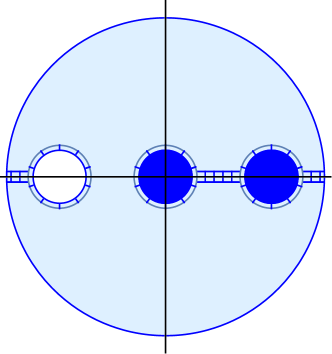
An example of such (symmetric) tiling with two families is presented in Figure 4, $\mathcal{D}=\{D_{1}\},$ $\mathcal{B}=\{B_{1},B_{2}\}$, where $D_{1}$ is a white disc and $B_{1},B_{2}$ are blue discs.

Proposition 4.25.

Let $D$ be a closed disc with a piecewise smooth boundary, $\mathcal{D}=\{D_{i}\subset D,i=1,\ldots,{k_{1}}\}$ and $\mathcal{B}=\{B_{j}\subset D,j=1,\ldots{k_{2}}\}$ families of smooth disjoint closed discs, which can be also empty, i.e. $k_{1}=0$ or $k_{2}=0.$ Set $\Delta:={D}\setminus\mathrm{int}(D_{1}\cup\ldots\cup D_{k_{1}}\cup B_{1}\cup\ldots\cup B_{k_{2}})$ and let $V\subset\partial\Delta$ be a discrete set of points containing all nonsmooth points of $\partial D$. Let $\delta>0$ be given.

Then there exists a $\delta$-tiling $\mathcal{T}_{\Delta}$ of $\Delta,$ so that the vertices of the tiling are disjoint from $V.$ More precisely,

$$\mathcal{T}_{\Delta}=\mathcal{T}_{\mathcal{B}}\underrightarrow{\cup}\mathcal{T}\underrightarrow{\cup}\mathcal{T}_{\mathcal{D}},$$

where $\mathcal{T}_{B}$ is a $\delta$-tiling of the $\mathcal{B}$-necklace, $\mathcal{T}_{D}$ is a $\delta$-tiling of the $\mathcal{D}$-necklace and $\mathcal{T}$ is a tiling of the closure of the set $\Delta$ with tiles from $\mathcal{T}_{\mathcal{B}}$ and $\mathcal{T}_{\mathcal{D}}$ removed.

Proof.

Let $\mathcal{T}_{\mathcal{B}}$ be an ordered $\delta$-tiling of the $\mathcal{B}$-necklace, $\mathcal{T}_{\mathcal{D}}$ an ordered $\delta$-tiling of the $\mathcal{D}$-necklace with the vertices of both tilings disjoint from $V.$ Define $T_{B}:=\cup_{T\in\mathcal{T}_{B}}T,$ $T_{D}:=\cup_{T\in\mathcal{T}_{D}}T,$ and let $K:=\Delta\setminus(\mathring{T_{B}}\cup\mathring{T_{D}})).$ The set $K$ needs to be tiled.

Assume that $k_{1},k_{2}>0.$ The set $K$ is a topological disc with a piecewise smooth boundary and can be mapped by a map, smooth up to the boundary (except at finitely many points, where it is only continuous) to the model square $Q=[-1,1]\times[1,3]$ of Example 4.16, Figure 3 (b), in such a way that $\partial K\cap T_{B}$ is mapped to $[-1,1]\times\{1\}$ and $\partial K\cap T_{D}$ is mapped to $[-1,1]\times\{3\}.$ As $\delta$-tiling $\mathcal{T}$ of $K$ consider the one induced by a fine enough tiling of the model square $Q$. We may assume that the images of vertices of $\mathcal{T}_{B}$ and $\mathcal{T}_{D}$ and the images of set $V$ are not the endpoints of horizontal and vertical segments of the grid of $Q.$ Then $\mathcal{T}_{B}\underrightarrow{\cup}\mathcal{T}\underrightarrow{\cup}\mathcal{T}_{D}$ is the desired tiling of $K.$

If $k_{1}=0$ (or $k_{2}=0$) we apply the same argument without the requirements that the $\partial K\cap T_{B}$ (or $\partial K\cap T_{D}$) is mapped to the edge $[-1,1]\times\{1\}$ (or $[-1,1]\times\{3\}$).

4.4. Proof of Theorem 4.17

Since the problem for axially symmetric domains which are not slice domains will be covered as a subproblem for slice domains, we assume that $\Omega_{I}$ is a slice domain.

We will apply a procedure following two steps: by Proposition 4.3 we first exhaust $\Omega_{I}$ by symmetric compact sets $\{K_{n}\}_{n\in\mathbb{N}_{0}}$ with smooth boundaries and then proceed by induction. Once the tiling $\mathcal{T}_{n}$ of $K_{n}$ is defined, we extend it to the tiling of $K_{n+1}$ by tiling the set $K_{n+1}\setminus\mathring{K_{n}}$ in the following manner: we first extend the tiling of ${K}_{n}$ with a tiling of $K_{n+1}\setminus\mathring{(K^{\bullet}_{n})}$ (extension outwards) and then we extend the new tiling with a tiling of the set $K^{\bullet}_{n}\cap\mathring{K}_{n+1}$ (extension inwards).

The initial tile is $T_{0}=K_{0}$; recall that $K_{0}\cap\mathbb{R}\neq\varnothing$. For the induction step, let $\mathcal{T}_{n}$ be the symmetric tiling of $K_{n}$ which is already defined. Observe that because the covering is locally finite, there exists $\delta_{n+1}>0$ such that for each $z\in K_{n+1}$ the disc $B(z,\delta_{n+1})$ is contained in all of the open sets of the covering $\mathcal{U}_{I}$ that intersect $B(z,\delta_{n+1})$. Fix such a $\delta_{n+1}.$ In order to satisfy the condition that the tiling is subordinated to the given covering it suffices to construct tiles such that their connected components have diameter less than $\delta_{n+1}.$

Denote the union of connected components of $K_{n},$ which intersect the real axis by $K_{n}^{\prime},$ and the union of those which do not by $K_{n}^{\prime\prime}.$ Hence $K_{n}=K_{n}^{\prime}\cup K_{n}^{\prime\prime},$ similarly $K_{n+1}=K_{n+1}^{\prime}\cup K_{n+1}^{\prime\prime};$ analogously, for the filled components of $K_{n},$ we set ${K}^{\bullet}_{n}={K}^{\prime\bullet}_{n}\cup{K}^{\prime\prime\bullet}_{n},$ where ${K}^{\prime\bullet}_{n}$ (resp. ${K}^{\prime\prime\bullet}_{n}$) denote the union of filled components of $K_{n}$ that intersect (resp. do not intersect the real axis). Notice that $(K_{n}^{\prime})^{\bullet}=(K^{\bullet}_{n})^{\prime},$ $(K_{n}^{\prime\prime})^{\bullet}=(K^{\bullet}_{n})^{\prime\prime}.$

Let $K_{n+1,\nu}$ be a connected component of $K_{n+1}.$ Put $K_{-1}:=K_{n}\cap K_{n+1,\nu}.$ We extend the tiling to the set ${K_{n+1,\nu}}$ in two steps. First we extend the tiling to ${K_{n+1,\nu}}\setminus\mathring{K}_{-1}^{\bullet}$ (outwards) and then to ${K}_{-1}^{\bullet}\cap K_{n+1,\nu}$. (inwards).

We also distinguish two cases: (1) if the set $K_{n+1,\nu}$ is in the upper half-plane, we extend the tiling from $K_{n}$ to $K_{n+1,\nu}$ and then extend it to ${K_{n+1,\nu}}\cup R(K_{n+1,\nu})$ by reflection over the real axis; (2) if $K_{n+1,\nu}$ intersects the real axis, it is symmetric and hence we have to extend the symmetric tiling of $K_{n}$ to a symmetric tiling $K_{n+1,\nu}.$

Case 1: $K_{n+1,\nu}\subset K_{n+1}^{\prime\prime}.$ Then either $K_{n+1,\nu}\subset\mathbb{C}_{I}^{+}$ or $K_{n+1,\nu}\subset\mathbb{C}_{I}^{-}$ and without loss of generality we assume that $K_{n+1,\nu}\subset\mathbb{C}_{I}^{+}.$ By Remark 4.11 it suffices to define the tiling of $K_{n+1,\nu}$ and then extend it to ${K_{n+1,\nu}}\cup R(K_{n+1,\nu})$ by reflection.

Consider the set $K_{n+1,\nu}\cup{K}^{\bullet}_{-1}.$ It is a topological closed disc with finitely many holes $D_{1},\ldots D_{k_{1}}$ and contains (at most) finitely many closed discs $B_{1},\ldots B_{k_{2}}$ which are all the connected components of ${K}^{\bullet}_{-1}.$ Put $K:=K_{n+1,\nu}^{\bullet},$ $\mathcal{D}=\{D_{1},\ldots D_{k_{1}}\},$ $\mathcal{B}=\{B_{1},\ldots B_{k_{2}}\}.$

(i) Extending the tiling outwards. Proposition 4.25 with $D:=K$ and families $\mathcal{B},\mathcal{D}$ of closed discs yields the desired tiling, so that the vertices of the new grid that are on the set $K_{-1}$ are different from the ones on $\partial K_{-1}$ induced by the tiling of $K_{n}.$

(ii) For the extension of the tiling inwards it suffices to explain the construction for one of the discs $B\in\mathcal{B},$ since they are disjoint.

If $B$ is a connected component of $K_{n},$ it is already tiled and there is nothing to do. Hence, assume that $B$ is not a connected component of $K_{n}$ and therefore $B\cap K_{n}$ has at least one hole. Because $K_{n}$ is Runge in $K_{n+1}$ also the intersection $B\cap K_{n+1,\nu}$ has at least one smaller hole in each hole of $B\cap K_{n}$. Let $D_{1}^{\prime},\ldots,D^{\prime}_{k_{1}}$ be the holes of $K_{n+1,\nu}$ contained in $B$. Take a small disc $B(p,r)\Subset D_{1}^{\prime}$ and reflect the set $B\cap K_{n}$ across the circle $\partial B(p,r).$ The reflection transforms the problem of extending inwards to the problem of extending outwards and by (i) we can extend the tiling.

Case 2: $K_{n+1,\nu}\subset K_{n+1}^{\prime}.$ Also in this case we proceed in a similar manner. First we fill outwards and then inwards.

Consider the set $K_{n+1,\nu}\cup{K}^{\bullet}_{-1}.$ It is a symmetric closed disc with finitely many holes $D_{1},\ldots D_{k_{1}}$ and contains (at most) finitely many closed symmetric discs $B_{1},\ldots B_{k_{2}}$ which are connected components of ${K}^{\bullet}_{-1}.$ Recall that the tiling of $K_{n}$ implies that there are vertices of $\partial B_{j}$ to be avoided.

(i) Extending the tiling outwards. Form a complete (symmetric) necklace of all $D_{i}$ and $B_{j}$ that contain real points and let the symmetric $\delta_{n+1}-$ tiling of the necklace be given by Remark 4.24 with vertices disjoint from vertices on tilings contained in the discs $B_{j}$. In the case of trivial necklace, tile the line segment. Define the set $V$ as the set of the vertices of this tiling of the necklace. Remove the union of the tiles from the set $K_{n+1,\nu}\setminus\mathring{(K^{\bullet}_{-1})}$ and define $D$ to be the connected component of the new set in the upper half-plane. So $D$ is a closed disc with a piecewise smooth boundary which contains all the remaining discs $B_{j}$ and has all the remaining holes $D_{i}.$ As before, we collect them in the families $\mathcal{B}$ and $\mathcal{D}.$ The Proposition 4.25 for $D$ and the set of vertices $V$ yields the desired tiling.

(ii) It remains to extend the tiling inwards, i.e. to tile the set $(K_{-1}^{\bullet}\cap K_{n+1,\nu})\setminus\mathring{K_{n}}.$ Choose a connected component $B$ of $K_{-1}^{\bullet}.$ If $B$ is a connected component of $K_{n},$ it is already tiled and there is nothing to do. Hence, assume that $B$ is not a connected component of $K_{n}.$

If $B$ is in the upper (or lower) half-plane, then Case 1 applies.

Assume that $B$ intersects the real axis. As before, $K_{n}\cap B$ equals $B$ with finitely many holes and each of them contains a hole of $K_{n+1,\nu}$ (see Figure 5(a)). Since the holes of $K_{n}\cap B$ are disjoint, each one can be filled separately so we may assume that there is either a pair of symmetric holes (Figure 5(b) on the right) and then Case 1 applies or there is only one (Figure 5(b), the light blue disc with centre at the origin) and intersects the real axis. Assume the latter and denote the hole by $D^{\prime}.$ Our aim is to extend the tiling to the set $D^{\prime}\cap K_{n+1,\nu}$.

The set $(D^{\prime}\cap K_{n+1,\nu})\cup(K_{n}\cap D^{\prime})^{\bullet}$ equals $D^{\prime}$ with holes $D_{1},\ldots,D_{k_{1}}$ and contains filled components $B_{1},\ldots,B_{k_{2}}$ of $K_{n}\cap D^{\prime}.$ It may happen, that $k_{2}=0,$ but since $D^{\prime}$ is a hole of $K_{n},$ $k_{1}$ is necessarily strictly positive. If $D_{1}$ is a hole on the real axis, then by reflection across small circle $S(a,r)\subset D_{1},$ centered at the real axis, we transform the case to the first part of Case 2, (filling outwards).

Refer to captionRefer to captionRefer to caption(a)(b)(c)Refer to captionRefer to captionRefer to captionmissing-subexpressionmissing-subexpression𝑎𝑏𝑐missing-subexpressionmissing-subexpression\begin{array}[]{ccccc}{\includegraphics[width=130.08731pt]{IntTiling.pdf}}&{\includegraphics[width=130.08731pt]{LadyBug1.pdf}}&{\includegraphics[width=130.08731pt]{LadyBugTiled1.pdf}}\\ (a)&(b)&(c)\end{array}

Figure 5. (a) the set $B\cap K_{n+1,\nu}$, (b) the set $K_{n}\cap B$ (blue), already tiled, with a hole $D$ (light blue centered in the origin) that intersects the real axis and with a pair of symmetric holes (light blue), filled components of $K_{n}$ (dark blue), domain to be tiled (light blue) and holes of $K_{n+1}$ (white), (c) the symmetric tiling of the symmetric necklace.

If there is no hole on the real axis, then we form a symmetric (possibly trivial) necklace with the filled components of $K_{n}$ contained in $D^{\prime},$ which intersect the real axis (Figure 5(c)) and extend the already constructed tiling with the tiling of the necklace. Remove the union of tiles of this tiling of the necklaces from the set $D^{\prime},$ denote the closure of the connected component in the upper half-plane by $K^{\prime}$ and by $V$ the set of vertices of the tiling in $\partial K^{\prime}.$ Then it suffices to extend the tiling to $K^{\prime}$ and reflect it over the real axis to obtain the tiling of $D^{\prime}\cap K_{n+1,\nu}.$

Recall that the outer boundary of $K^{\prime}$ is already contained in the tiling, but since there is at least one hole in $K^{\prime}$, the associated family of holes, $\mathcal{D}$, is not empty, we extend the existing tiling with the one provided by Proposition 4.25 for the set $K^{\prime}$ in the place of $D,$ the family $\mathcal{D}$ (and the family $\mathcal{B}$ of filled connected components of $K_{n}$, if it exists). Observe that in this manner we do get the extension of the tiling, because the last tiles are added around the holes and therefore it does not happen that the last tile intersects the union of the previously added tiles in a closed curve.

Notice that since $D^{\prime}$ itself may contain the filled components of $K_{n}\cap D^{\prime},$ which are not connected components of $K_{n}$, we have to proceed inductively to extend the tiling to $(K_{n}\cap D^{\prime})^{\bullet}\cap K_{n+1,\nu}$. Since there are only finitely many of them, the process stops and defines a (finite) tiling of the compact set $K_{n+1}.$ This completes the induction step.∎

5. Applications to antisymmetric homology groups of symmetric planar domains

As for the holomorphic case, one has to take into account that the slice–preserving quaternionic $\exp$ has some periodicity, but this periodicity only applies when $\exp$ is restricted to a slice $\mathbb{C}_{I}$ and cannot be extended automatically; to be more precise, the function $f(z)=\exp(z+2\pi i)$ is periodic in $\mathbb{C}_{i}$ but it is no longer slice–preserving (it is only $\mathbb{C}_{i}$ preserving), hence the periodicity of the (extension) of the function $f$ to $\mathbb{H}$ is not preserved. On the hand the function $\exp(z)$ is $2\pi\mathcal{I}$– periodic in $\mathbb{H}\setminus\mathbb{R}$.

In order to give a consistent definition of fundamental domains of $\exp$ and its restrictions $\exp_{I}$ on each slice $\mathbb{C}_{I}$, it is convenient to extend the lattice $i\mathbb{Z}$ in $\mathbb{C}_{i}$ and consider the (image of) $\mathcal{I}\mathbb{Z}$ in $\mathbb{H}$ as its generalization. Observe that, if $z\in\mathbb{H}\setminus\mathbb{R}$, then

(5.2) $$\mathcal{I}(z)=-\mathcal{I}(\overline{z}).$$

In what follows, we are going to investigate the periods of quaternionic exponential function in the perspective of looking for solutions of the multiplicative quaternionic Cousin problems. In a more general setting these problems can be formulated in terms of vanishing of properly defined cohomology groups, which the authors will present in a forthcoming paper.

As usual, we proceed by first restricting the problem to slices. The property (5.2) instructs as to consider antisymmetric functions on symmetric domains in $\mathbb{C}$.

Definition 5.1 (Antisymmetric complexes and cohomology groups).

Let $D\subset\mathbb{C}$ be an open symmetric set and $\mathcal{U}=\{U_{\lambda}\}_{\lambda\in\Lambda}$ an open symmetric covering of $D$. An antisymmetric $m$-cochain of $\mathcal{U}$ is any collection $\{(f_{L},U_{L}),f_{L}:U_{L}\rightarrow\mathbb{Z}\}_{L\in\Lambda^{m}}$ with $f_{L}$ continuous, constant in $U_{L}^{+}$ and satisfying the antisymmetric property:

$$f_{L}(z)=-f_{L}(\bar{z}).$$

Antisymmetric cochain complexes and coboundary operators are defined as usual and corresponding cohomology groups denoted by $H^{n}_{a}(\mathcal{U},\mathbb{Z})$. The open symmetric coverings of $D$ form a directed set under refinement, therefore we define $H^{n}_{a}(D,\mathbb{Z})$ to be a direct limit over symmetric open coverings of $D$.

Notice that the definition of the antisymmetric $m$-cochain implies that $f_{L}=0$ whenever $U_{L}\cap\mathbb{R}\neq\varnothing$.

Theorem 5.2 (Vanishing of antisymmetric cohomology groups).

Let $D\subset\mathbb{C}$ be a symmetric open set. Then

$$H^{n}_{a}(D,\mathbb{Z})=0\mbox{ for all }n\geq 2.$$
Proof.

Take $n=2$. Without loss of generality we may assume, by Theorem 1.1, that there exists a Cartan covering ${\mathcal{U}}$ of $\widetilde{D}\subset\mathbb{H},$ which defines an open symmetric covering $\mathcal{U}_{I}$ when restricted to $\mathbb{C}_{I}\cong\mathbb{C}$ and that the antisymmetric cocycle $C_{coc}$ is given by

$$C_{coc}=\{(f_{klm},U_{klm,I}),f_{klm}:U_{klm,I}\rightarrow\mathbb{Z}\}_{k,l,m\in\mathbb{N}_{0}}.$$

We would like to show that $C_{coc}$ is a coboundary, i.e. there exists an antisymmetric cochain $C=\{(f_{kl},U_{kl,I}),f_{kl}:U_{kl,I}\rightarrow\mathbb{Z}\}_{k,l\in\mathbb{N}_{0}}$ which is mapped to $C_{coc}$ by the coboundary operator.

By definition, if $U_{klm,I}$ consists of two symmetric components, $U_{klm,I}=U_{klm,I}^{+}\cup U_{klm,I}^{-}$, then $f_{klm}$ equals $n_{klm}$ on $U_{klm,I}^{+}$ and $-n_{klm}$ on $U_{klm,I}^{-}.$

Define a new covering $\mathcal{V}=\{V_{\kappa}\}_{\kappa\in\mathbb{N}_{0}}$, where the open sets are the connected components of the sets $U_{k,I}$, i.e. the sets $U_{k,I}^{0}:=U_{k,I}$ if connected and the sets $U_{k,I}^{+}$ and $U_{k,I}^{-}$ otherwise.

We define the cocycle $C_{I}:=\{(\nu_{\kappa\lambda\mu},V_{\kappa\lambda\mu})\}_{\kappa,\lambda,\mu\in\mathbb{N}_{0}}$ in $\Omega_{I}$ in the following manner. If $V_{\kappa}$ is a connected component of $U_{k,I},$ $V_{\lambda}$ a connected component of $U_{l,I}$, $V_{\mu}$ a connected component of $U_{m,I}$, then we set

$$\nu_{\kappa\lambda\mu}:=\left\{\begin{array}[]{rl}n_{klm},&\mbox{ if }\quad V_{\kappa\lambda\mu}\subset\mathbb{C}_{I}^{+},\\ -n_{klm},&\mbox{ if }\quad V_{\kappa\lambda\mu}\subset\mathbb{C}_{I}^{-},\\ 0,&\mbox{ if }\quad V_{\kappa\lambda\mu}\cap\mathbb{R}\neq\varnothing,\end{array}\right.$$

because if $V_{\kappa\lambda\mu}\cap\mathbb{R}\neq\varnothing,$ we know that $n_{klm}=0.$

Since we know that $H^{2}(\Omega_{I},\mathbb{Z})$ is trivial, the cocycle $C_{I}$ is a coboundary, hence there exists a cochain $C_{1}:=\{(\nu_{\kappa\lambda},V_{\kappa\lambda})\}_{\kappa,\lambda\in\mathbb{N}}$ so that $\nu_{\kappa\lambda\mu}=\nu_{\kappa\lambda}+\nu_{\lambda\mu}+\nu_{\mu\kappa}$ in $V_{\kappa\lambda\mu}$.

We are looking for an antisymmetric cochain; in principle there is no reason that if $V_{\kappa}=U_{k,I}^{+},$ $V_{\lambda}=U_{l,I}^{+}$ and $V_{\kappa_{1}}=U_{k,I}^{-},$ $V_{\lambda_{1}}=U_{l,I}^{-},$ we also have $\nu_{\kappa\lambda}=-\nu_{\kappa_{1}\lambda_{1}}.$ Using the notation above we define a new cochain by setting ${\mu}_{\kappa\lambda}:=-\nu_{\kappa_{1}\lambda_{1}}$ (and ${\mu}_{\kappa_{1}\lambda_{1}}:=-\nu_{\kappa\lambda});$ in the cases $V_{\kappa}=U_{k,I}^{0},$ $V_{\lambda}=U_{l,I}^{+},$ $V_{\kappa_{1}}=V_{\kappa}=U_{k,I}^{0},$ $V_{\lambda_{1}}=U_{l,I}^{-}$ and $V_{\kappa}=U_{k,I}^{0},$ $V_{\lambda}=U_{l,I}^{0},$ $V_{\kappa_{1}}=V_{\kappa}=U_{k,I}^{0},$ $V_{\lambda_{1}}=V_{\lambda}=U_{l,I}^{0}$ the definition is analogous. Set $N_{\kappa\lambda}=(\nu_{\kappa\lambda}+{\mu}_{\kappa\lambda})/2.$ Then by construction $N_{\kappa\lambda}=-N_{\kappa_{1}\lambda_{1}}.$ In particular, if $V_{\kappa\lambda}\cap\mathbb{R}\neq\varnothing,$ $V_{\kappa\lambda}$ is its own reflection and $N_{\kappa\lambda}=0.$

Since the covering is symmetric, the cochain $C_{2}:=\{({\mu}_{\kappa\lambda},V_{\kappa\lambda}),\kappa,\lambda\in\mathbb{N}\}$ is mapped to the cocycle $C_{I}$ and hence also cochain $C_{3}:=\{(N_{\kappa\lambda},V_{\kappa\lambda}),\kappa,\lambda\in\mathbb{N}\}$ is mapped to $C_{I}$ by the coboundary mapping.

To define the cochain $C=\{(f_{kl},U_{kl,I}),k,l\in\mathbb{N}\}$ we proceed as follows. If $U_{kl,I}\cap\mathbb{R}\neq\varnothing$, then, by assumption on symmetry, it is its own reflection image and (by definition of $\mathcal{V}$) it equals some $V_{\kappa\lambda};$ we set $n_{kl}=N_{\kappa\lambda}(=0).$ Let $V_{\kappa}\subset U_{k,I}$, $V_{\lambda}\subset U_{l,I}$. If $U_{kl,I}\cap\mathbb{R}=\varnothing,$ then $U_{kl,I}=U_{kl,I}^{+}\cup U_{kl,I}^{-}.$ If $U_{kl,I}^{+}=V_{\kappa\lambda}$ then define $f_{kl}:=N_{\kappa\lambda}$ on $U_{kl,I}^{+}$ and $f_{kl}:=-N_{\kappa\lambda}$ on $U_{kl,I}^{-}$. If $U_{kl,I}^{-}=V_{\kappa\lambda}$ then define $f_{kl}:=N_{\kappa\lambda}$ on $U_{kl,I}^{-}$ and $f_{kl}:=-N_{\kappa\lambda}$ on $U_{kl,I}^{+}$. This implies that $C$ is indeed an antisymmetric cocycle that is mapped to $C_{coc}$ by a coboundary operator thus making $C_{coc}$ a coboundary.

If $n\geq 3,$ the groups $H^{n}_{a}(D,\mathbb{Z})$ are trivial, because there exist arbitrarily fine Cartan coverings and they have order at most $3$, which means that no four distinct sets of such a covering intersect. ∎

References

  • [AdF1] A. Altavilla, C. de Fabritiis, *-exponential of slice regular functions, Proc. Amer. Math. Soc. 147, 1173–1188, 2019.
  • [AdF2] A. Altavilla, C. de Fabritiis, *-logarithm for slice regular functions, Atti Accad. Naz. Lincei Cl. Sci. Fis. Mat. Natur. 34, no. 2, 491–-529 2023.
  • [BW] C. Bisi, J. Winkelmann, On Runge pairs and topology of axially symmetric domains, J. Noncommut. Geom. 15, 2, 713–-734, 2021
  • [FP] F. Forstnerič, J. Prezelj, Oka’s principle for holomorphic submersions with sprays, Math. Ann., 322 (4), 633–666, 2002.
  • [GPV] G.Gentili, J.Prezelj, F. Vlacci, On a definition of logarithm of quaternionic functions, J. Noncommut. Geom. 17 (3), 1099–-1128, 2023.
  • [GSS] G. Gentili, C. Stoppato, D. Struppa, Regular functions of a quaternionic variable, Springer Monographs in Mathematics, Springer, Heidelberg, 2013.
  • [GS] G. Gentili, D. Struppa, A new theory of regular functions of a quaternionic variable, Adv. Math., 216, 279–301, 2007.
  • [GMP] R. Ghiloni, V. Moretti, A. Perotti, Continuous slice functional calculus in quaternionic Hilbert spaces, Rev. Math. Phys. 25 (4), :1350006,83, 2013.
  • [GP] R. Ghiloni, A. Perotti, Slice regular functions of several Clifford variables, Proceedings of ICNPAA 2012 - Workshop “Clifford algebras, Clifford analysis and their applications”, AIP Conf. Proc. 1493, 734–738, 2012
  • [GR] R.C. Gunning, H. Rossi, Analytic Functions of Several Complex Variables, AMS Chelsea publishing, American Mathematical Society. Providence, Rhode Island, 2009
  • [HL] G. Henkin, J. Leiterer, The Oka-Grauert principle without induction over the basis dimension. Math. Ann.  311, 71–93, 1998.