Enhancing Reinforcement Learning in Sensor Fusion: A Comparative Analysis of Cubature and Sampling-based Integration Methods for Rover Search Planning
Abstract
This study investigates the computational speed and accuracy of two numerical integration methods, cubature and sampling-based, for integrating an integrand over a 2D polygon. Using a group of rovers searching the Martian surface with a limited sensor footprint as a test bed, the relative error and computational time are compared as the area was subdivided to improve accuracy in the sampling-based approach. The results show that the sampling-based approach exhibits a deviation in relative error compared to cubature when it matches the computational performance at . Furthermore, achieving a relative error below necessitates a increase in relative time to calculate due to the complexity of the sampling-based method. It is concluded that for enhancing reinforcement learning capabilities and other high iteration algorithms, the cubature method is preferred over the sampling-based method.
I Introduction
Machine Learning (ML) has gained massive popularity in the last decade[1] driven by both the ongoing research into learning algorithms and cheap computational performance[2]. Phenomenon such as the success of generative artificial intelligence[3] have put ML more into the eye of the public than ever before. However, behind the scenes, researchers spend a vast amount of time preparing data for learning. All three major forms of ML require high-quality data for the best performance: supervised learning needs well-labelled data points, unsupervised learning must have noise-free data for labeling, and reinforcement learning has to have access to a good representation of the environment. Studies on the impact of non-systematic noise on training have shown massively degraded performance [4, 5].
A lot of research effort is dedicated to increasing the robustness of ML algorithms against noise [6], or even creating new ones specifically for noisy training [7]. However, in the realm of reinforcement learning noise can be beneficial. Action noise, which is the addition of randomness to the action selected by the algorithm, can be desirable to encourage exploration of the action space. Using Gaussian or Ornstein-Uhlenbeck noise has been shown to significantly improve training across popular reinforcement algorithms such as Soft Actor-Critic [8] or Deep Deterministic Policy Gradient [9] when coupled with scheduled noise reduction [10]. However, this scheduling shows that noise must be minimized to fine-tune the model. In comparison, observation noise in reinforcement learning, akin to poor-quality labelled data for supervised learning, is known to make training unstable [11]. Noise in ML, when not controllable, is undesirable as it increases the difficulty in successfully learning a model.
A famously noisy task is numerical integration. From Euler integration to complex modern algorithms, errors are inevitable compared to continuous methods as numerical methods are just approximations. However, reducing these errors is paramount to decreasing noise. It is very common to have simulation step updates within a reinforcement learning environment which require integration in multiple forms. This might be double integrating acceleration to get the position, or integrating a function within a 2D shape. The latter is what this research focuses on. This problem takes the form
| (1) |
where , is the integrand, and is the collection of -simplices. In search path planning, the integrand is commonly a Probability Distribution Map (PDM), and is the path buffered by the sensor footprint . A widely used method of integration is a sampling-based approach which calculates the integration result through grid sampling of the PDM and then calculating the summation of pixels within . A different approach uses cubature [12] to achieve a similar result. This relies on the transformation of into a sum of computable simplices such as triangles or rectangles. The works by [13] implement methods for 15 primitive regions that any simplex can be dissected into, like the aforementioned triangle and rectangle. The integration result is then the sum of cubature results for each simplex.
The task of numerically integrating an integrand over a 2D shape within search planning can be thought of as ”How much probability has been seen by executing this mission?” In this application, the integrand is a PDM that defines the probability of detection at a given point and the 2D shape is the search path buffered by some quantity to get a polygon. To apply reinforcement learning to this problem, the newly observed probability could be used to calculate the reward function. As previously outlined, this requires a fast and noiseless numerical integration method for good training characteristics.
Search planning typically is applied in situations where exhaustive search (also known as coverage planning) is infeasible due to mission constraints such as limited resources. One such situation where a reduced vehicle lifespan is the limiting factor is searching the Martian surface for items of scientific interest based on a PDM. In 2020, NASA’s Mars Mission utilized two robots: the Perseverance rover and the Ingenuity helicopter - opening the door to the use of collaborative robotic teams for planetary exploration [14]. The use of multi-rover teams for planetary exploration missions has been considered in terms of both surface [15] and cave [16] exploration. By using a team of planetary exploration rovers, the data collection capabilities of a mission can be increased due to the extended sensor footprint.
In this study, the two aforementioned integration methods are benchmarked against each other to determine the performance differences between them. This will inform future studies on which method is appropriate for their application. A group of rovers searching the Martian landscape with reduced sensor footprints is used as a benchmark. The generated paths are highly irregular due to collision avoidance and inter-rover communications creating a challenging 2D polygon to integrate over. The PDM for this scenario is analogous to the probability distribution of a meteor that has crashed on the surface and that the rovers are now searching for.
The top-level mission planning and environment generation is introduced in Sect. II-A, with modelling and path planning in Sect. II-B. Sampling-based and cubature integration is defined in Sect. II-C1 and Sect. II-C2 respectively. The results are presented and discussed in Sect. III with a conclusion being drawn in Sect. IV.
II Method
II-A Mission Planning
The PDM is modelled as a sum of bivariate Gaussians[17] such that a point on the surface of Mars at coordinate has a probability of containing the meteor p
| (2) |
where and are the mean location and covariance matrix of the th bivariate Gaussian respectively. For this study, these values are randomly generated with . [18] used a similar method to approximate a discrete PDM through a Gaussian mixture model which employs Eq. \tagform@2 for the final .
This PDM is then used in conjunction with LHC_GW_CONV [19] to generate mission waypoints with a search radius of . The area is and is thus segmented into a grid such that each cell is the size of the search radius.
LHC_GW_CONV is, at its core, a greedy algorithm by employing the local hill climb (LHC) optimization method. This evaluates all eight surrounding cells and moves to the highest-scoring one. If there is a tie, a convolution kernel centred around the offending cells is evaluated and the cell with the highest score
| (3) |
is selected. A normalized box blur kernel is typically used and is defined as
| (4) |
Furthermore, LHC does not handle multi-modal problems well as it attempts to cover one mode completely before being able to move to the next. This often leads to LHC ignoring much more rewarding modes. To solve this, global warming (GW) is introduced. This works by subtracting from the PDM a number of times, where and is the global maxima. This then gives the updated PDM
| (5) |
which the LHC uses to generate a new path. After all GW steps are evaluated, they are scored using the original PDM and the path with the highest accumulated probability is selected.
Finally, each visited cell is marked a seen, and subsequent evaluations of at this cell will return . This discourages revisiting a position but does not entirely forbid it.
II-B Rover Modelling and Path Planning
II-B1 Mars Map Generation
A 3D terrain model has been created using data from the High-Resolution Imaging Science Experiment (HiRISE) on the Mars Reconnaissance Orbiter. The map is a matrix of latitude, longitude, and elevation data, and has a resolution of per pixel [20]. For this work, a mission site has been selected from within the Jezero crater. The generated mission site consists of a block grid. Fig. 1 shows the 3D terrain model that has been generated, based on previous work at the University of Glasgow [21].
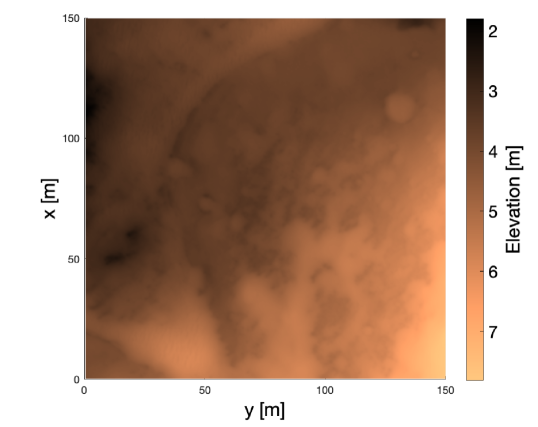
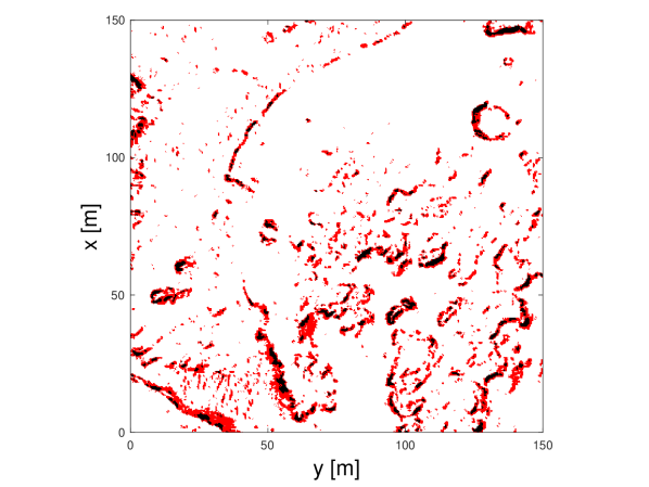
The 3D terrain model is analysed in terms of the elevation of neighbouring blocking in the grid. A given block inherits the worst-case slope angle, , from its eight neighbouring blocks. Three traversability categories have been defined: traversable (), high-risk (), and impassable (). The thresholds of the three traversability categories have been set in line with the nominal operational limits of the Perseverance rover [22]. Fig. 2 shows the resulting traversability map for the selected mission site.
II-B2 Rover Model
The robot utilised for analysis and testing in this work is the rocker bogie runt (RBR). This rover has a small form factor (), and a six-wheel rocker bogie suspension in line with the baseline mobility characteristics of current planetary exploration robotos [23]. The RBR has six wheels; three wheels on each side, where a front wheel is connected to the rocker, and the middle and rear wheels are connected to the bogie. Each of the six wheels is driven by its own 6V DC motor. Unlike NASA’s Mars rovers, which utilise steerable wheels, all RBR wheels are fixed and cannot rotate. Therefore, the differential drive steering method is used. For this work, a team of five rovers is utilised, each with a search footprint diameter of .
II-B3 Generating Safe Paths
The paths of each member of the rover team must be coordinated such that no collisions occur between them as they traverse paths toward their respective targets. As planetary exploration rovers operate in such remote and hazardous environments, collisions could cause the loss of the rovers involved and severe degradation to the group’s data collection capabilities.
For each target point generated by LHC_GW_CONV, a set of safe paths is generated using prioritised planning coordination [24]. Each rover path is given an arbitrary priority number. A path planning attempt is then made for the first rover, using RRT*. A simulation of the rover is run to obtain 4D pose data. The path of the second rover the then planned, and its behaviour is simulated. The 4D pose data for both rovers is compared to check for collisions. If a collision occurs, the path of the lower priority rover is re-planned until a safe path is found. If no collisions occur, the path is saved and the algorithm moves to the next rover. This process continues until all five rovers have safe paths.
II-C Path Analysis
Each rover generates a unique path as it executes the mission which is buffered by the search footprint diameter . The total search area is then the union of the set of buffered paths such that
| (6) |
This can be extended to be a function of time by
| (7) |
where is the set of buffered paths covered by the rovers up until . If is the time taken for the entire mission to be completed, it then follows that and .
II-C1 Sampling-based Integration
Accessing the value of at a given coordinate is trivial, and is as computationally expensive as the definition of itself. A harder task is determining if the point at is within .
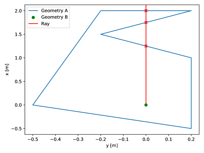
A popular method is ray casting along a straight line from a point [25]. If this ray intersects (geometry B in the example seen in Fig. 3) an odd amount of times then the point is contained by the buffered search paths.
Another popular method uses the Dimensionally Extended Nine Intersection Matrix (DE-9IM)[26]. This is calculated using
| (8) |
where is the dimension of ( if , and if ), and the superscripts , , and denote the interior, boundary, and exterior regions respectively. This matrix can be used to calculate different predicates for and to be in. The predicate of interest here is the topological within, which is described by the pattern matrix
| (9) |
where an entry in the matrix is marked if , if , and if .
The DE-9IM approach is faster than the ray-casting method when dealing with the high-vertex polygons generated by the buffered paths and is the method used for the rest of this study.
As touched on in Sect. I, the sampling method is the sum of pixels within the polygon written as
| (10) |
where and are the dimensions of the rasterisation, is the area enclosed by the rasterisation, is the integrand (akin to from Eq. \tagform@1) which is a function accessing the pixel value at , and is a single polygon. This method can be fast with low values of and , and accurate with high values alike. However, this method highly suffers from aliasing around the borders of . Methods to get around the aliasing problem have been tried [27] with major performance penalties. Nonetheless, due to its simplicity, it is prominently used in the literature [18, 28, 29, 30, 31].
II-C2 Cubature Integration
The simplex must first be subdivided into a set of the 15 primitive simplices [13], with the simplest and most ubiquitous of these being the triangle. As is likely to have many holes and unlikely to be convex, the constrained Delaunay triangulation [chew_constrained_1989] is used to get the set of triangles .
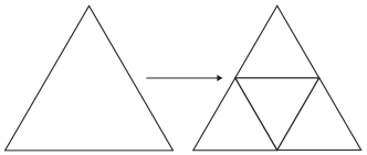
At the beginning of the algorithm, the integration estimate and error estimate is evaluated for every triangle in where the unit triangle is transformed to the given triangle, while the cubature formula maintains its given degree. To calculate , the cubature formula of polynomial degree 13 with 37 points [32] is used. is calculated using several null rules as defined in [33]. If (where are user-defined absolute and relative error tolerances respectively) is above the tolerance set, the triangle with the highest error is subdivided into four smaller triangles as seen in Fig. 4. Each new triangle has its integral and error estimates evaluated, and the four replace the original triangle. This process is continued until either is below the tolerance, or a maximum number of calculations has been exceeded.
III Results
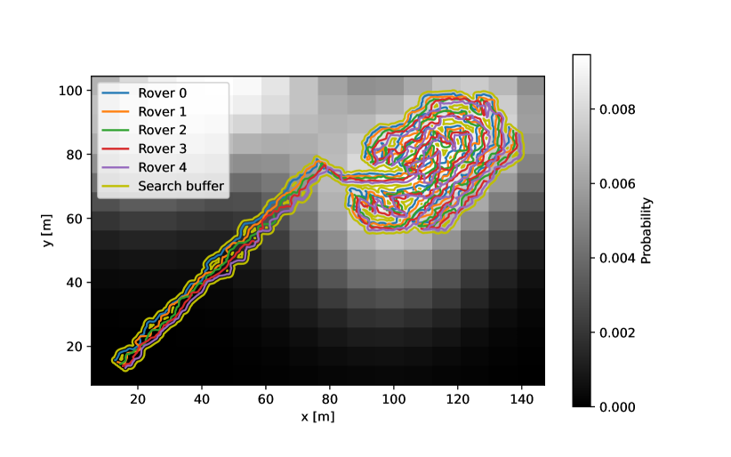
As discussed in Sect. II-A, LHC is a greedy algorithm that prioritizes local modes. This can be seen in Fig. 5 at where the mission abruptly leaves the saddle between the modes to ascend the local probability mode. The rovers attempt to avoid collision and obstacles, creating small holes in the buffered search path as well as a highly irregular exterior. This creates a challenging benchmark to compare and contrast the methods.
To benchmark the methods, the cubature method is evaluated for each PDM and corresponding paths and the mean of this result (time and integration result) was deemed the baseline. Overall, missions have been simulated using the mission planning from Sect. II-A and the rover simulation from Sect. II-B. In this case, the sampling method is evaluated from to , and the relative error and relative time are calculated with
| (11) |
where and are the cubature and sampling values respectively.
From Eq. \tagform@10, it can be seen that the grid that the sampling method uses grows in . For the remainder of this study, for simplicity making this algorithm . This is evident from Fig. 6 where it can be seen that after , the cubature method is as fast to compute as the sampling method. After , this value is at . For reinforcement learning, where billions of steps are taken in the modelled environments during training, this can quickly add days to the learning time.
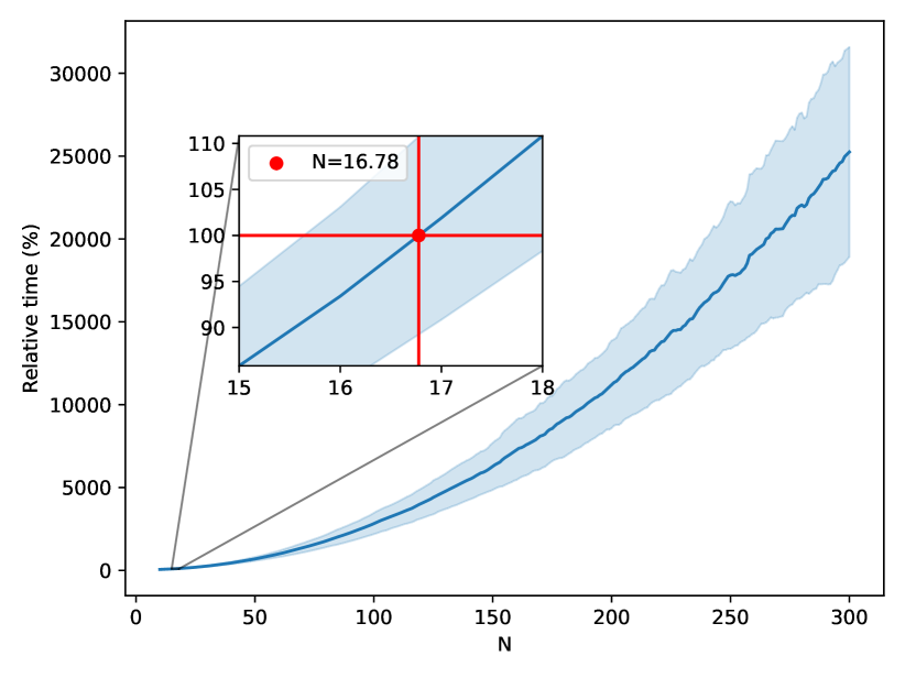
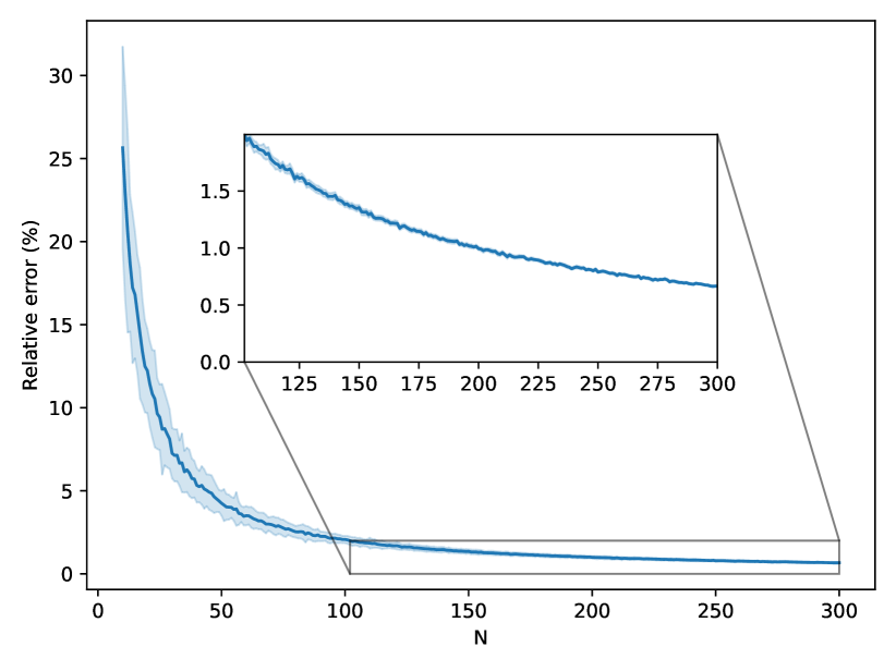
Fig. 7 shows the exponential decay of the relative error as increases. At the crossing point of , the relative error is . Depending on the application, this level of accuracy might be deemed sufficient. However, for reinforcement learning, as outlined in Sect. I, any noise is to be mitigated as it can lead to unstable training and therefore diminished results. Even at the high value of , the relative error is still above . This size of error is likely to be acceptable, however the computational cost is too high to justify this method.
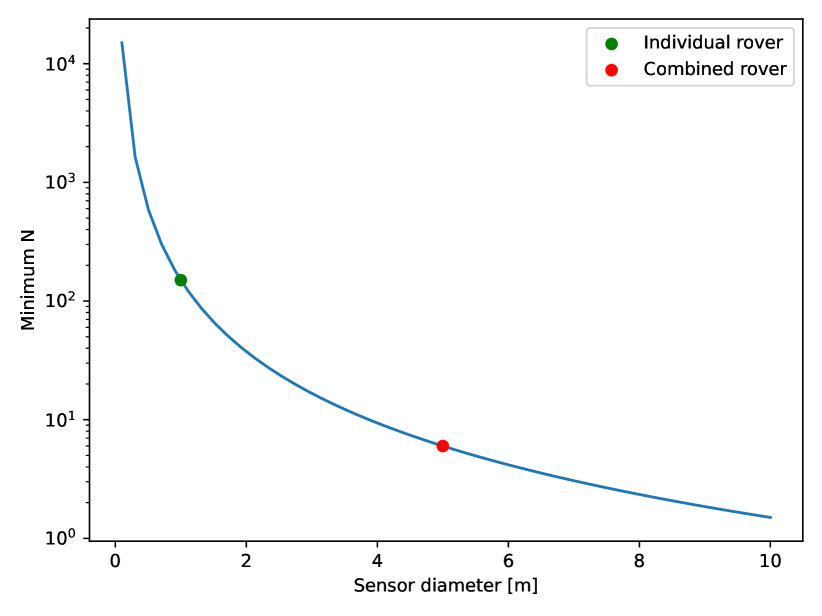
A smaller might lead to faster computation, the physical meaning of must be considered. The individual rovers have a sensor diameter of and the area has dimensions . To ensure that each grid cell is the same size as that of a single rover’s sensor, which would lead to a relative time difference between the two methods.
The impact of the varying maximum number of coordinates per trial, denoted as , on the relative error was examined to ensure it was not a dependent variable. The null hypothesis posited that does not affect the relative error. Following the application of an ordinary least squares, a -value of was computed surpassing the level of significance (). Thus, the null hypothesis cannot be rejected indicating that there is no significant evidence to suggest that influences the relative error.
IV Conclusion
This study presents a comprehensive analysis comparing cubature and sampling-based integration of an integrand over a 2D polygon. An example scenario requiring the search of an area on Mars by a coordinated group of rovers was used as a test bed. These rovers completed a search mission created from the integrand; a random PDM. The union of the resultant buffered paths was then used as the 2D polygon. Using the trajectories from missions, the aggregated data analysis showed that the cubature approach is substantially more accurate and significantly faster. Both of these qualities are important within reinforcement learning, where marginal performance gains can quickly snowball into days of saved training time. Furthermore, these results also translate to embedded devices where the computational budget is typically limited. This could be the case for the likes of onboard navigation systems on a self-sufficient rover similar to the one used in this research.
Overall, the results of this study highlight the superiority of the cubature approach in terms of accuracy and computational efficiency, particularly in scenarios requiring coordinated search missions like those encountered in reinforcement learning and embedded systems for autonomous navigation. However, it’s important to acknowledge the limitations of this work. While the focus was on comparing two prevalent integration methods, numerous other techniques warrant exploration. Additionally, the requirement of a continuous integrand for the cubature method may pose challenges in certain scenarios, though potential solutions using approximations have been discussed. By recognizing these limitations, future research can build upon these findings to further enhance integration techniques for a wide range of applications.
References
- [1] I. H. Sarker, “Machine Learning: Algorithms, Real-World Applications and Research Directions,” SN Computer Science, vol. 2, no. 3, p. 160, May 2021.
- [2] M. I. Jordan and T. M. Mitchell, “Machine learning: Trends, perspectives, and prospects,” Science, vol. 349, no. 6245, pp. 255–260, Jul. 2015.
- [3] C. Stokel-Walker and R. Van Noorden, “What ChatGPT and generative AI mean for science,” Nature, vol. 614, no. 7947, pp. 214–216, Feb. 2023.
- [4] D. F. Nettleton, A. Orriols-Puig, and A. Fornells, “A study of the effect of different types of noise on the precision of supervised learning techniques,” Artificial Intelligence Review, vol. 33, no. 4, pp. 275–306, Apr. 2010.
- [5] J. R. Quinlan, “Induction of decision trees,” Machine Learning, vol. 1, no. 1, pp. 81–106, Mar. 1986.
- [6] Y. Guo and W. Wang, “A robust adaptive linear regression method for severe noise,” Knowledge and Information Systems, vol. 65, no. 11, pp. 4613–4653, Nov. 2023.
- [7] R. Fox, A. Pakman, and N. Tishby, “Taming the Noise in Reinforcement Learning via Soft Updates,” Mar. 2017.
- [8] T. Haarnoja, A. Zhou, P. Abbeel, and S. Levine, “Soft Actor-Critic: Off-Policy Maximum Entropy Deep Reinforcement Learning with a Stochastic Actor,” Aug. 2018.
- [9] T. P. Lillicrap, J. J. Hunt, A. Pritzel, N. Heess, T. Erez, Y. Tassa, D. Silver, and D. Wierstra, “Continuous control with deep reinforcement learning,” Jul. 2019.
- [10] J. Hollenstein, S. Auddy, M. Saveriano, E. Renaudo, and J. Piater, “Action Noise in Off-Policy Deep Reinforcement Learning: Impact on Exploration and Performance,” Jun. 2023.
- [11] K. Sun, Y. Zhao, S. Jui, and L. Kong, “Exploring the Training Robustness of Distributional Reinforcement Learning Against Noisy State Observations,” in Machine Learning and Knowledge Discovery in Databases: Research Track, ser. Lecture Notes in Computer Science, D. Koutra, C. Plant, M. Gomez Rodriguez, E. Baralis, and F. Bonchi, Eds. Cham: Springer Nature Switzerland, 2023, pp. 36–51.
- [12] J. Lyness and R. Cools, “A Survey of Numerical Cubature over Triangles,” Proceedings of Symposia in Applied Mathematics American Mathematical Society Providence, RI, vol. 48, Apr. 1994.
- [13] R. Cools, L. Pluym, and D. Laurie, “Algorithm 764: Cubpack++: A C++ package for automatic two-dimensional cubature,” ACM Transactions on Mathematical Software, vol. 23, no. 1, pp. 1–15, Mar. 1997.
- [14] K. Farley, K. Williford, and K. e. a. Stack, “Mars 2020 mission overview,” Space Science Reviews, vol. 216, no. 142, 2020.
- [15] T. Fong, B. D. Allen, and S. Azimi, “Autonomous systems & robotics for lunar surface infrastructure,” in AIAA ASCEND, 2021.
- [16] T. Vaquero, M. Troesch, and S. Chien, “An approach for autonomous multi-rover collaboration for mars cave exploration: Preliminary results,” in International Symposium on Artificial Intelligence, Robotics, and Automation in Space (i-SAIRAS 2018), Madrid, Spain, June 2018.
- [17] P. Yao, Z. Xie, and P. Ren, “Optimal UAV Route Planning for Coverage Search of Stationary Target in River,” IEEE Transactions on Control Systems Technology, vol. 27, no. 2, pp. 822–829, Mar. 2019.
- [18] L. Lin and M. A. Goodrich, “Hierarchical Heuristic Search Using a Gaussian Mixture Model for UAV Coverage Planning,” IEEE Transactions on Cybernetics, vol. 44, no. 12, pp. 2532–2544, Dec. 2014.
- [19] ——, “UAV intelligent path planning for wilderness search and rescue,” 2009 IEEE/RSJ International Conference on Intelligent Robots and Systems, IROS 2009, vol. 0, no. 1, pp. 709–714, 2009.
- [20] J. W. Bergstrom, W. Delamere, and A. McEwen, “Mro high resolution imaging science experiment (hirise): Instrument test, calibration and operating contrainst,” in 55th International Astronautical Congress of the International Astronautical Federation, the International Academy of Astronautics, and the International Institute of Space Law, 2004, pp. Q–3.
- [21] M. Baxter, “Modelling and visualisation of the mars terrain for rover simulations,” Master’s thesis, University of Glasgow, 2022.
- [22] A. Rankin, M. Maimone, J. Biesiadecki, N. Patel, D. Levine, and O. Toupet, “Driving curiosity: Mars rover mobility trends during the first seven years,” in 2020 IEEE Aerospace Conference. IEEE, 2020, pp. 1–19.
- [23] T. Flessa, E. W. McGookin, and D. G. Thomson, “Taxonomy, systems review and performance metrics of planetary exploration rovers,” in 2014 13th International Conference on Control Automation Robotics & Vision (ICARCV). IEEE, 2014, pp. 1554–1559.
- [24] S. Swinton and E. McGookin, “A Novel, RRT* Based Approach to the Coordination of Multiple Planetary Rovers,” in 2022 UKACC 13th International Conference on Control (CONTROL), Apr. 2022, pp. 88–93.
- [25] I. E. Sutherland, R. F. Sproull, and R. A. Schumacker, “A Characterization of Ten Hidden-Surface Algorithms,” ACM Computing Surveys, vol. 6, no. 1, pp. 1–55, Mar. 1974.
- [26] E. Clementini, P. Di Felice, and P. Van Oosterom, “A small set of formal topological relationships suitable for end-user interaction,” in Advances in Spatial Databases, G. Goos, J. Hartmanis, D. Abel, and B. Chin Ooi, Eds. Berlin, Heidelberg: Springer Berlin Heidelberg, 1993, vol. 692, pp. 277–295.
- [27] J.-H. Ewers, D. Anderson, and D. Thomson, “Optimal path planning using psychological profiling in drone-assisted missing person search,” Advanced Control for Applications, p. e167, Sep. 2023.
- [28] M. Morin, I. Abi-Zeid, and C.-G. Quimper, “Ant colony optimization for path planning in search and rescue operations,” European Journal of Operational Research, vol. 305, no. 1, pp. 53–63, Feb. 2023.
- [29] A. Subramanian, R. Alimo, T. Bewley, and P. Gill, “A Probabilistic Path Planning Framework for Optimizing Feasible Trajectories of Autonomous Search Vehicles Leveraging the Projected-Search Reduced Hessian Method,” in AIAA Scitech 2020 Forum, AIAA. Orlando, FL: American Institute of Aeronautics and Astronautics, Jan. 2020.
- [30] D. Ebrahimi, S. Sharafeddine, P.-H. Ho, and C. Assi, “Autonomous UAV Trajectory for Localizing Ground Objects: A Reinforcement Learning Approach,” IEEE Transactions on Mobile Computing, vol. 20, no. 4, pp. 1312–1324, Apr. 2021.
- [31] L. Hong, Y. Wang, Y. Du, X. Chen, and Y. Zheng, “UAV search-and-rescue planning using an adaptive memetic algorithm,” Frontiers of Information Technology & Electronic Engineering, vol. 22, no. 11, pp. 1477–1491, Dec. 2011.
- [32] S. Wandzurat and H. Xiao, “Symmetric quadrature rules on a triangle,” Computers & Mathematics with Applications, vol. 45, no. 12, pp. 1829–1840, Jun. 2003.
- [33] J. Berntsen and T. O. Espelid, “Algorithm 706: DCUTRI: An algorithm for adaptive cubature over a collection of triangles,” ACM Transactions on Mathematical Software, vol. 18, no. 3, pp. 329–342, Sep. 1992.