Influence of Organic Molecules and Phosphate Ions on the Formation of Biosilica Patterns in Diatoms

The formation of regularly structured silica valves in diatoms is a captivating process in biomineralization. Specific organic molecules, including long-chain polyamines, silaffins, and silacidins, have been found to be essential in this process. The molecular structure of synthesized polyamines greatly affects the quantity, size, and shape of silica precipitates. Experimental findings indicate that silica precipitation occurs at specific concentrations of phosphate ions, with higher concentrations resulting in larger aggregates of organic molecules that serve as templates for silica formation.

Our study focuses on the hypothesis that pattern formation in diatom valve structures is driven by the phase separation of species-specific organic molecules, with the evolving organic structures acting as templates for silica deposition. We specifically investigate the role of phosphate ions in the self-assembly of long-chain polyamines and analyze how their reaction with organic molecules impacts the morphology of the organic template. By varying the model parameters, including degree of dissociation and initial concentrations of reacting components, we show that the resulting geometric features of the patterns are highly dependent on these factors.

Furthermore, we explore the scenario where an initial array of organic droplets serves as a static template for silica deposition, considering the effects of "prepatterning" by the silica costae in the base layer. We obtain numerical solutions that generate a diverse range of two-dimensional patterns closely resembling the valve structures observed experimentally.

1 Introduction

Diatoms, with their intricately designed silica valves, have secrets that could revolutionize science and transform our world. They are a type of unicellular algae well studied for the formation of biological silica. They are found in aquatic environments with sufficient sunlight and minerals. Their cell walls, comprising two thecae adorned with intricately shaped valves and girdle bands[33], serve multifaceted functions. They offer mechanical strength to resist shear stress and for protection against predators[11, 18, 14], and nutrient filtration[17]. The valves themselves are constructed using a system of silica ribs connected by tiny silica bridges, resulting in self-supporting structures that utilize minimal silica. In addition, the valves in the areas between the ribs exhibit distinctive patterns characterized by self-similar pores.

Diatoms, often called the "lungs of our planet", are of great ecological importance. These minuscule wonders are pivotal actors in the global carbon cycle[28, 38] and have a significant impact on climate regulation. They make a great contribution to oxygenation of the air we breathe[1, 3], highlighting their vital role in the maintenance of human existence.

However, diatoms have even greater potential. They have exceptional optical and electrical properties that remain largely unexplored. Their meticulously designed silica valves exhibit optical qualities similar to those of natural microlenses[10, 12], diffracting light in a manner reminiscent of photonic crystals[21]. This unique characteristic can be used in a wide range of optical applications, from advanced imaging systems to innovative sensor technologies[32].

Beyond their optical qualities, diatom silica valves are sustainable, cost-effective[40], and eco-friendly materials[41]. The renewable nature of diatoms and their biomineralization process stand as a compelling paradigm for sustainable materials production. Diatom-based materials have potential in biosensors[27, 32], drug delivery systems[46, 30, 13], and as supportive materials for advanced technological devices[31]. Their distinctive properties, including photoluminescence[20], give them significant value in a wide range of applications.

Unlocking the secrets of diatom morphogenesis is important in addressing climate change, developing renewable energy, creating advanced materials, enhancing biomedicine, and much more. Equipped with this knowledge, we can envision a future that is greener, healthier, and more sustainable.

The formation of diatom cell walls occurs within specialized compartments known as silica deposition vesicles (SDVs). Silicic acid, a soluble form of silica, is taken up by silicon transporters into the SDV where it is precipitated. To maintain high intracellular concentrations of silicic acid, diatoms use sophisticated mechanisms to prevent uncontrolled precipitation. The proposal that organic components interact with silicic acid to stabilize it within silica transport vesicles (STVs) provides insight into the formation of silica spheres, which promote cell wall growth[34].

Recent advances in diatom research have elucidated the molecular mechanisms that underlie pore pattern morphogenesis in diatom silica [19]. This fascinating process begins during the early stages of costae formation and centers around organic droplets within valve silica deposition vesicles (SDVs). During this stage, the space between the silica ribs does not contain silica, but organic droplets are formed through a liquid-liquid phase separation process. These droplets, positively charged because of long-chain polyamines (LCPAs), arrange themselves along the negatively charged silica rib edges, maintaining a uniform spacing via electric repulsion. As they take positions, they provide the basis for the formation of the cribrum matrix, which covers the entire intervening space of the silica ridges except where the organic droplets are located.

The silica precursor enters the space between the ribs, although its precise composition remains uncertain. The silica nanoparticles found in SDVs hint at their potential role as feedstock for silica growth in the SDV. At this stage, organic droplets act as templates, preventing infiltration of the silica precursor and guiding the formation of pores. The unique precursor pores exhibit wave-like peaks and anvil-shaped features, which emerge as a result of organic droplets arresting silica deposition. Silicification begins at the edges of the ribs and advances toward the opposing silica ribs. The matrix of the cribrum plate is continuously silicified.

Chemical analysis of diatom biosilica have elucidated a diverse set of organic components, including carbohydrates, lipids, amino acids, and proteins, particularly $\alpha 1$ -frustulin, which is related to the biosilica matrix [39]. The formation of silica structures is influenced by species-specific organic molecules, such as long-chain polyamines, silaffins, and silacidins, which play a key role in templating the silica deposition [29, 24].

Studies have indicated that the molecular structure of synthesized polyamines significantly impacts the amount, size, and morphology of silica precipitates [4]. Furthermore, the role of phosphate ions is essential in the process of silica precipitation [36, 4, 43]. In these studies, the pH threshold required for silica precipitation has been shown to depend on the phosphate concentration [36]. The higher concentrations of phosphate lead to the formation of larger spherical aggregates of organic molecules, which serve as templates for silica formation upon the addition of silicic acid molecules to the solution [36]. Size control of polyamine aggregates can be achieved by adjusting the pH value at a fixed polyamine/phosphate ratio [36]. Furthermore, an experimental study on silaffins in [23] showed that unlike natSil-1A, silaffin 1-A could not induce silica precipitation without phosphate. Considering these experimental insights, it becomes evident that the interaction between organic molecules and phosphate ions significantly influences the phase separation of organic molecules.

Considerable strides have been made in elucidating the complex chemical and biological processes involved in the silica morphogenesis of diatom valves. Despite these advances, the field of theoretical modeling for diatom valve morphogenesis remains relatively underexplored.

One of the pioneering theories proposed diffusion-limited aggregation (DLA) of silica nanoparticles at the leading edges of the SDV as a model for silica rib formation [16]. This model described the random fluctuation of silica particles in a fluid environment, leading to dendritic structures. It suggested that a nucleation structure in the center of the SDV initiates the formation of silica ribs, with aggregation and sintering processes involved.

Laterally dependent stochastic aggregation (LSDA) model, probabilistic model, which focus on silica precipitation and dissolution rates at solid/fluid interfaces, provided valuable insights into porous structures [44]. Negative lateral feedback in the solid regions promoted pore formation, while fluid regions encouraged silicification. Potential chemical reagents inside SDVs were suggested to control this feedback.

The hypothesis of organic molecules guiding silica pattern formation within SDVs introduced the concept of liquid-liquid phase separation as a mechanism for pattern template formation [35, 26, 5]. Models suggested that these processes create organic phases with silica precipitation activity and aqueous phases containing silica precursors. Silica precipitates around organic droplets, forming pore cavities. The work carried out in [26] yielded numerous two-dimensional patterns that closely resembled the observed valve structures, where phase separation was induced by an additional local field arising from pre-existing silica costae in the base layer. Another more recent model [5], which coupled phase separation with a chemical reaction, aimed to study the role of phosphate ions in the self-assembly of LCPAs. While two- and three-dimensional simulations of pattern formation were presented, the influence of model parameters on the morphology of the organic template remains unclear.

Building upon these previous works, our study seeks to elucidate the roles of organic molecules and phosphate ions in the formation of diatom valve silica. Expanding on the framework in [5], which couples phase separation with chemical reactions, our aim is to demonstrate how the model parameters influence pattern formation.

This paper is structured as follows: Firstly, in order to study the role of phosphate ions in the aggregation process, we introduce a comprehensive mathematical model of the phase separation of organic molecules coupled with a chemical reaction. Subsequently, we examine the free energy associated with this process using the Flory-Huggins model. Following this, we conduct a linear stability analysis of the model equations to obtain the necessary conditions for pattern formation. The next section is devoted to numerical simulations to study the various stationary patterns that are obtained. Furthermore, we analyze the influence of confined geometry, model parameters, and prepatterning field on the resulting patterns.

2 Model

Our research aims to analyze the aggregation of organic molecules. In order to comprehend the influence of phosphate ions on this phenomenon, we have decided to study a simplified and generic chemical reaction:

$$A+B\overset{\beta}{\underset{\alpha}{\leftrightarrows}}C,$$ (1)

where $A$ represents organic molecules that cannot undergo phase separation. We assume that when phosphate ions (component $B$) bind to these organic molecules, a new organic component (component $C$) is formed with a higher level of phosphorylation, see [5]. This increased phosphorylation decreases the charge of component $C$, making it more likely to phase separate. The dynamics of the system (1) is determined by the continuity equation:

$$\cfrac{\partial\mathbf{c}}{\partial t}=-\nabla\cdot\mathbf{j}+\mathbf{r},$$ (2)

where $\mathbf{c}=(c_{A},c_{B},c_{C})$, with $c_{A}$, $c_{B}$ and $c_{C}$ as concentrations of the chemical components $A$, $B$ and $C$, respectively; $\mathbf{j}$ denotes spatial fluxes, which for simplicity will be driven by diffusive process for species $A$ and $B$; $\mathbf{r}$ denotes the source term related to chemical reactions that convert new organic component into a mixture of solvent and organic molecules able to phase separate. The chemical reactions are local, described by rate laws (depending on the composition).

The source term $\mathbf{r}$ is defined by (1). The reaction velocity of the components $A$ and $B$ is described by the coefficient $\alpha$, and the reverse reaction (dissociation of the component $C$) is described by the coefficient $\beta$. Therefore, from (1) it follows:

$$\mathbf{r}=(-\alpha c_{A}c_{B}+\beta c_{C},-\alpha c_{A}c_{B}+\beta c_{C},\alpha c_{A}c_{B}-\beta c_{C}).$$

For organic molecules and phosphate ions the diffusion flux $\mathbf{j}$ is given by Fick’s law. Therefore, the evolution of the concentrations of components $A$ and $B$ is described by the following reaction-diffusion equations:

$$\cfrac{\partial c_{A}}{\partial t}=\nabla\cdot D_{A}\nabla c_{A}-\alpha c_{A}c_{B}+\beta c_{C}$$ (3)

$$\cfrac{\partial c_{B}}{\partial t}=\nabla\cdot D_{B}\nabla c_{B}-\alpha c_{A}c_{B}+\beta c_{C},$$ (4)

where $D_{A}$ and $D_{B}$ are the diffusion coefficients, which are typically dependent on concentrations $c_{A}$, $c_{B}$ and $c_{C}$ and the charge state of the polymer. However, because specific information on the studied polyamine-phosphate ion-water system is not available, we assume in this analysis that these kinetic coefficients are constant.

To describe the phase separation process of the component $C$ we use the Cahn-Hilliard model. The volume fraction $\phi$ of the component $C$ is related to the concentration by $\phi=\Omega_{c}c_{C}$ with $\Omega_{c}$ as the molecular volume. This model is particularly useful for understanding the thermodynamic behavior of the system, and it allows us to study the effects of different parameters on the phase separation process. The thermodynamic state of phase separating component is governed by the free energy:

$$F[\phi]=\int\left(f(\phi)+\cfrac{\kappa}{2}(\nabla\phi)^{2}\right)dV,$$ (5)

where $\phi(\mathbf{r})$ is the volume fraction of component $C$, $f(\phi)$ is the free energy density of mixing and $\kappa$ is the gradient energy coefficient (assumed to be constant).

For component $C$, non-local diffusive fluxes $j$ are driven by a gradient in the chemical potential. Linear non-equilibrium thermodynamic implies $j=-M(\phi)\nabla\mu$, where $M$ is the positive mobility (for simplicity, it is approximated as a constant) and $\mu$ is the chemical potential. Hence we obtain

$$\cfrac{\partial\phi}{\partial t}=\nabla\cdot\left(M\nabla\mu\right)+\alpha c_{A}c_{B}-\beta\phi.$$ (6)

Together with the constraint $\cfrac{1}{V}\int dV\phi(\mathbf{r})=\overline{\phi}$ and since $\mu=\delta F/\delta\phi$, we obtain the evolution equation for volume fraction $\phi(\mathbf{r},t)$:

$$\cfrac{\partial\phi}{\partial t}=\nabla\cdot M\nabla\left(f^{\prime}(\phi)-\kappa\nabla^{2}\phi\right)+\alpha c_{A}c_{B}-\beta\phi.$$ (7)

We employ the Flory-Huggins free energy density:

$$f(\phi)=kT\left[\cfrac{1}{N}\phi\ln\phi+(1-\phi)\ln(1-\phi)+\chi\phi(1-\phi)\right],$$ (8)

where $k$ is the Boltzmann constant, $T$ is the absolute temperature, $N$ is the length of polymer in units of the solvent size and $\chi$ is the Flory-Huggins interaction parameter.

In this study, the notion of spinodal decomposition is used. It refers to the process in which a single thermodynamic phase naturally splits into two phases without the need for nucleation. This separation occurs in the absence of any thermodynamic barrier to the phase separation. Spinodal decomposition is observed when the second derivative of the free energy density is negative, denoted as $f^{\prime\prime}(\phi)<0$.

To make the equations dimensionless, we introduce the length unit $l=\sqrt{\kappa/(kT)}$, the time unit $\widehat{t}=t/\tau$ with $\tau=l^{2}/(M(kT))$, $\widehat{\nabla}=l\nabla$, and $\widehat{f}=f/(kT)$. This allows us to express the reaction-diffusion equations (3),(4) for $c_{A}$, $c_{B}$ multiplying by $\Omega_{C}$ and the evolution equation (7) for the volume fraction $\phi$ in a dimensionless form:

$$\cfrac{\partial\widehat{c}_{A}}{\partial\widehat{t}}=\widehat{\nabla}\cdot\widehat{D}_{A}\widehat{\nabla}\widehat{c}_{A}-\widehat{\alpha}\widehat{c}_{A}\widehat{c}_{B}+\widehat{\beta}\phi$$ (9)

$$\cfrac{\partial\widehat{c}_{B}}{\partial\widehat{t}}=\widehat{\nabla}\cdot\widehat{D}_{B}\widehat{\nabla}\widehat{c}_{B}-\widehat{\alpha}\widehat{c}_{A}\widehat{c}_{B}+\widehat{\beta}\phi$$ (10)

$$\cfrac{\partial\phi}{\partial\widehat{t}}=\widehat{\nabla}^{2}\left(\widehat{f}^{\prime}(\phi)-\widehat{\nabla}^{2}\phi\right)+\widehat{\alpha}\widehat{c}_{A}\widehat{c}_{B}-\widehat{\beta}\phi,$$ (11)

where $\widehat{c}_{A}=\Omega_{C}c_{A}$, $\widehat{c}_{B}=\Omega_{C}c_{B}$ are concentrations $c_{A}$ an $c_{B}$ scaled by the molecular volume of component $C$; $\widehat{D}_{A}=D_{A}\tau/l^{2}$, $\widehat{D}_{B}=D_{B}\tau/l^{2}$, $\widehat{\alpha}=\alpha\tau/\Omega_{C}$ and $\widehat{\beta}=\beta\tau$. This is the model used in [5].

We solve numerically the system of nonlinear partial differential equations (9)-(11), which describe the coupled evolution of the three components. To conduct simulations in a confined geometry, we utilized the finite element software Comsol Multiphysics. Our phase separation model is distinguished by six model parameters $\chi$, $N$, $D_{A}$, $D_{B}$, $\alpha$, and $\beta$, together with the initial concentrations $c_{A,0}$ and $c_{B,0}$. Given the significant number of parameters involved, our initial analysis focuses on determining the conditions under which a uniform system becomes unstable, leading to spinodal decomposition.

3 Flory-Huggins model

Before diving into the analysis of linear stability, we will thoroughly examine the free energy using the Flory-Huggins model.

The Flory-Huggins model stands as a fundamental theoretical framework that elucidates the intricate behavior of liquid-liquid phase separation, which emerges from the interplay between entropy and interaction energy. In this particular model, we examine the blending of a polymer species of length $N$ with a homogeneous solvent. The Flory-Huggins model employs an effective lattice site contact energy between the polymer and solvent, denoted as $\chi\equiv\cfrac{z}{2}\cfrac{2\epsilon_{ps}-\epsilon_{ss}-\epsilon_{pp}}{kT}$ in which $z$ is a coordination constant, and $\epsilon_{ps}$, $\epsilon_{ss}$ and $\epsilon_{pp}$ are bare polymer-solvent, solvent-solvent and polymer-polymer contact energies. The free energy density of the Flory-Huggins model is represented in (8).

On examination of the right-hand side of (8), we discern that the first two terms signify the entropic free energy of mixing, while the third term represents the effective contact energy. The spinodal concentration defines the boundary between locally stable and unstable regions and can be precisely determined.

The free energy density becomes locally unstable when $f^{\prime\prime}(\phi)\leq 0$, and consequently the spinodal boundary $\phi^{*}$ is defined at the transition point $f^{\prime\prime}(\phi^{*})=0$

$$f^{\prime\prime}(\phi)=\cfrac{1}{N\phi}+\cfrac{1}{1-\phi}-2\chi.$$ (12)

Solving for this condition, we obtain the dense $(\phi^{s}_{1})$ and dilute phase $(\phi^{s}_{2})$ spinodal concentrations

$$\phi^{s}_{1,2}=\cfrac{1}{4\chi N}\left(N(2\chi-1)+1\pm\sqrt{(N(2\chi-1)+1)^{2}-8\chi N}\right).$$ (13)

The critical point of liquid-liquid phase separation occurs when the dense and dilute phases coincide, corresponding to a critical interaction strength $\chi^{*}$ and concentration $\phi^{*}$:

$$\chi^{*}=\cfrac{1}{2}\left(1+\cfrac{1}{N}+\cfrac{2}{\sqrt{N}}\right),\qquad\phi^{*}=\cfrac{\sqrt{N}+1}{N+1+2\sqrt{N}}.$$

Near the critical point with $\delta\chi\equiv\chi-\chi^{*}\approx 0$, the spinodal concentrations have the approximate form

$$\phi^{s}_{1,2}=\phi^{*}\pm\sqrt{\cfrac{\delta\chi}{2(\chi^{*})^{2}\sqrt{N}}}+O(\delta\chi).$$

Figure S1 illustrates how the Flory-Huggins interaction parameter affects the spinodal decomposition for a given value of $N$.

For simplicity of the model, we assume that the reaction and diffusion processes are faster than phase separation. Therefore, we start from the initial conditions:

$$\left.c_{A}\right|_{t=0}=c_{A,0},\qquad\left.c_{B}\right|_{t=0}=c_{B,0},\qquad\left.\phi\right|_{t=0}=0.$$

Following this, a rapid establishment of reaction equilibrium takes place:

$$\alpha c_{A,e}c_{B,e}=\beta\phi_{e}.$$

Considering the conservation law of the particles, we derive:

$$c_{A,0}=c_{A,e}+\phi_{e},\qquad c_{B,0}=c_{B,e}+\phi_{e}.$$

By considering both the initial and equilibrium conditions, we can deduce the equilibrium concentration of component $C$:

$$\phi_{e}=\cfrac{1}{2}\left(c_{A,0}+c_{B,0}+\cfrac{\beta}{\alpha}-\sqrt{\left(c_{A,0}+c_{B,0}+\cfrac{\beta}{\alpha}\right)^{2}-4c_{A,0}c_{B,0}}\right).$$ (14)

Keeping $\chi$ and $N$ fixed and substituting $\phi$ with $\phi_{e}$ in (12), we can examine $f^{\prime\prime}(\phi_{e}(c_{A,0},c_{B,0},\alpha,\beta))$. This allows us to determine the range of values for $c_{A,0}$, $c_{B,0}$, $\alpha$, $\beta$ within which spinodal decomposition occurs or our system remains stable, in other words, phase separation will not occur if the equilibrium volume fraction of the component $C$ lies outside the spinodal region of the free energy $(f^{\prime\prime}(\varphi_{e})<0)$.

Taking $N=10$ and $\chi=1.3$ in subsequent calculations, we find $\phi^{s}_{1,2}$ from (13). The set of plots presented in Fig. 1 elucidates the relationship between the equilibrium volume fraction of the component $C$ and the initial concentrations of organic molecules, phosphate ions, and the rate of the backward chemical reaction.

Keeping $c_{A,0}$ constant, we study the change in $\phi_{e}$ with respect to $c_{B,0}$ for different values of $\beta$, as shown in Fig. 1(a). A remarkable observation emerges: in a certain range of parameters on the graph, there is a region where the curves consistently lie below the concentration $\phi^{s}_{1}$ of the dense phase. This phenomenon means that spinodal degradation is excluded in this region, emphasizing the need for a minimum phosphate concentration to initiate spinodal degradation. Furthermore, an intriguing trend is observed: curves associated with higher values of $\beta$ descend onto the plot, implying that an increased concentration of $c_{B,0}$ is required for spinodal decomposition. Additionally, an increase in $c_{A,0}$ (see the Appendix) corresponds to a reduced requirement of $c_{B,0}$ for phase separation to take place. These findings provide valuable insight into the interplay of initial concentrations and dissociation coefficient that govern phase separation in the system.

We achieve analogous results in another set of curves presented in Fig. 1(b). Here, we explore the relationship between $\phi_{e}$ and $c_{B,0}$ for different values of $c_{A,0}$, while maintaining a constant coefficient of the backward reaction, $\beta$. When fixing the parameter $\beta$, our observations reveal that lower concentrations of $c_{A,0}$ require a higher concentration of $c_{B,0}$ to induce spinodal decomposition.

The comparison between the analytical results obtained from equations (13)-(14) and the numerical results obtained using the COMSOL Multiphysics software reveals that the theoretical predictions exhibit a wider range of parameters for spinodal decomposition compared to the numerical calculations, as presented in Fig. 1(d).

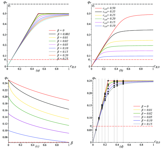
Figure 1: Equilibrium concentration of component $C$ depending on the reaction parameters at $N=10$ and $\chi=1.3$ for the case: $(a)$ $c_{A,0}=0.25$, $(b)$ $\beta=0.1$, $(c)$ $c_{B,0}=0.25$ and $(d)$ $c_{A,0}=0.25$. The dashed lines correspond to $\phi_{1}$ (red) and $\phi_{2}$ (black). Plot (d) compares the analytical results with the numerical results: the black dots represent spinodal decomposition, while the black cross indicates the absence of it in the numerical simulations.

4 Stability Analysis

Another approach to examine linear stability is to analyze whether small perturbations $(\delta c_{A},\delta c_{B},\delta\phi)$ to the equilibrium state of the system will grow or decay. By substituting $c_{a}=c_{A,e}+\delta c_{A}$, $c_{B}=c_{B,e}+\delta c_{B}$, and $\phi=\phi_{e}+\delta\phi$ into equations (9)-(11) (for simplicity, omitting the hat notation), we obtain the following equations for small fluctuations:

$$\cfrac{\partial\delta c_{A}}{\partial t}=D_{A}\nabla^{2}\delta c_{A}-\alpha(c_{A,e}\delta c_{B}+\delta c_{A}c_{B,e})+\beta\delta\phi$$ (15)

$$\cfrac{\partial\delta c_{B}}{\partial t}=D_{B}\nabla^{2}\delta c_{B}-\alpha(c_{A,e}\delta c_{B}+\delta c_{A}c_{B,e})+\beta\delta\phi$$ (16)

$$\cfrac{\partial\delta\phi}{\partial t}=\nabla^{2}(f^{\prime\prime}(\phi_{e})\delta\phi-\nabla^{2}\delta\phi)+\alpha(c_{A,e}\delta c_{B}+\delta c_{A}c_{B,e})-\beta\delta\phi$$ (17)

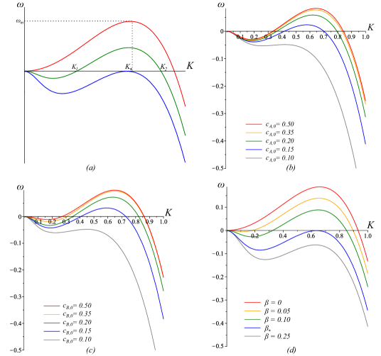
Figure 2: Dispersion relation $\omega(K)$: $(a)$ three scenarios, $(b)$ and $(c)$ for different initial concentrations of components $A$ and $B$, respectively, at $\beta=0.1$ and for $(b)$ $c_{B,0}=0.25$, for $(c)$ $c_{A,0}=0.25$; $(d)$ for different values of $\beta$ and $c_{A,0}=c_{B,0}=0.25$ revealing the strong impact of the dissociation constant on the spinodal decomposition. Shared parameters: $D_{A}=100$, $D_{B}=1000$, $\alpha=10$.

We seek a solution of the form:

$$\delta c_{A}=h_{A}\exp{\left(i(k_{1}x+k_{2}y)+\omega t\right)}$$

$$\delta c_{B}=h_{B}\exp{\left(i(k_{1}x+k_{2}y)+\omega t\right)}$$

$$\delta\phi=h_{C}\exp{\left(i(k_{1}x+k_{2}y)+\omega t\right)}$$

We aim to find a separable solution. By substituting the ansatz into equations (15)-(17), we obtain a set of equations for the amplitudes, which can be expressed in matrix form (2):

$$\begin{pmatrix}\omega+K^{2}D_{A}+\alpha c_{B,e}&\alpha c_{A,e}&-\beta\\ \alpha c_{B,e}&\omega+K^{2}D_{B}+\alpha c_{A,e}&-\beta\\ -\alpha c_{B,e}&-\alpha c_{A,e}&\omega+K^{2}(f^{\prime\prime}(\phi_{e})+K^{2})+\beta\end{pmatrix}\begin{pmatrix}h_{A}\\ h_{B}\\ h_{C}\end{pmatrix}=0$$ (18)

where $K^{2}=k_{1}^{2}+k_{2}^{2}$. To determine the solution to the linear system of homogeneous equations for the reaction-diffusion system, we calculate the determinant of the coefficient matrix. This results in a cubic equation for the growth rate $\omega$, which depends on the wave vector $K$:

$$\omega^{3}+\mathcal{G}(K^{2})\omega^{2}+\mathcal{P}(K^{2})\omega+\mathcal{V}(K^{2})=0$$ (19)

where

$$\mathcal{G}(K^{2})=K^{4}+\left(D_{A}+D_{B}+f^{\prime\prime}(\phi_{e})\right)K^{2}+\alpha(c_{A,e}+c_{B,e})+\beta$$ (20)

$$\mathcal{P}(K^{2})=K^{2}\left\{(D_{A}+D_{B})K^{4}+\left((D_{A}+D_{B})f^{\prime\prime}(\phi_{e})+D_{A}D_{B}+\alpha(c_{A,e}+c_{B,e})\right)K^{2}+\right.$$

$$\left.+D_{A}(\alpha c_{A,e}+\beta)+D_{B}(\alpha c_{B,e}+\beta)+\alpha(c_{A,e}+c_{B,e})f^{\prime\prime}(\phi_{e})\right\}$$ (21)

$$\mathcal{V}(K^{2})=K^{4}\left\{D_{A}D_{B}(K^{4}+K^{2}f^{\prime\prime}(\phi_{e})+\beta)+\alpha(D_{a}c_{A,e}+D_{B}c_{B,e})(K^{2}+f^{\prime\prime}(\phi_{e}))\right\}$$ (22)

In the region of interest within our parameter space, all three solutions of the equation are real. Two of these solutions consistently yield negative values across all wave vectors. The remaining solution, distinguished by positive values, is referred to the dispersion relation $\omega(K)$ that determines the growth rates for each mode with wavenumber $K$. In Fig. 2(a), distinct scenarios of characteristic growth rate are presented, each represented by a unique curve.

For wavenumber values $K$ where $w(K)>0$, the system becomes unstable, initiating spinodal decomposition. Generally, the function $w(K)$ transitions to negative values beyond a critical wavenumber $K_{*}$, marked by $\omega(K_{*})=0$. The blue curve in Fig. 2(a) represents a critical case in which the curve is entirely below the horizontal axis ($\omega=0$). Interestingly, it features a point of tangency with the $K$-axis, highlighting an equilibrium point at $\omega(K_{*})=0$ in the dispersion relation. In addition, it should be noted that fluctuations characterized by wavelengths shorter than $\lambda_{*}=2\pi/K_{*}$ decay as time progresses.

In this particular case, the model parameters must meet two essential conditions: first, they must satisfy equation (19), and second, the derivative of $\omega$ with respect to $K^{2}$ must equal zero, expressed as $\cfrac{d\omega}{dK^{2}}=0$. This implies that $\mathcal{V}$ and $\mathcal{V}^{\prime}_{K^{2}}$ must simultaneously be equal to zero. We obtain a quadratic equation for $K^{2}$:

$$K^{4}+\left(f^{\prime\prime}(\phi_{e})+\alpha\left(\cfrac{c_{A,e}}{D_{B}}+\cfrac{c_{B,e}}{D_{A}}\right)\right)K^{2}+\alpha\left(\cfrac{c_{A,e}}{D_{B}}+\cfrac{c_{B,e}}{D_{A}}\right)f^{\prime\prime}(\phi_{e})+\beta=0$$ (23)

When this equation possesses a repeated root, it introduces specific conditions necessary to attain patterning and determine the critical wavenumber:

$$\left\{\begin{aligned} &K^{2}_{*}=-\cfrac{1}{2}\left(\alpha\left(\cfrac{c_{A,e}}{D_{B}}+\cfrac{c_{B,e}}{D_{A}}\right)+f^{\prime\prime}(\phi_{e})\right)\\ &\left(\alpha\left(\cfrac{c_{A,e}}{D_{B}}+\cfrac{c_{B,e}}{D_{A}}\right)-f^{\prime\prime}(\phi_{e})\right)^{2}=4\beta\\ &-f^{\prime\prime}(\phi_{e})>\alpha\left(\cfrac{c_{A,e}}{D_{B}}+\cfrac{c_{B,e}}{D_{A}}\right)\end{aligned}\right.$$

On the second curve in Fig. 2(a), depicted in green, we observe a scenario where a portion of the plot extends above zero. This behavior results in two distinct roots corresponding to the exact points where the curve intersects the $K$-axis. Moreover, when the condition $\left(\alpha\left(\cfrac{c_{A,e}}{D_{B}}+\cfrac{c_{B,e}}{D_{A}}\right)-f^{\prime\prime}(\phi_{e})\right)^{2}>4\beta$ is satisfied, it signifies the existence of two roots for $\mathcal{V}(K^{2})=0$. In simpler terms, this condition implies the presence of two specific values, denoted as $K_{1,2}$, for which $\omega(K_{1,2})=0$:

$$K^{2}_{1,2}=-\cfrac{1}{2}\left\{f^{\prime\prime}(\phi_{e})+\alpha\left(\cfrac{c_{A,e}}{D_{B}}+\cfrac{c_{B,e}}{D_{A}}\right)\pm\sqrt{\left(\alpha\left(\cfrac{c_{A,e}}{D_{B}}+\cfrac{c_{B,e}}{D_{A}}\right)-f^{\prime\prime}(\phi_{e})\right)^{2}-4\beta}\right\}$$ (24)

The characteristic size of the initially emerging phase regions is defined by the wavelength $\lambda_{max}=2\pi/K_{max}$, where $K_{max}$ is the wave vector at which $\omega(K)$ reaches its maximum (see the red curve in Fig. 2(a)), determining the wavelength of the fastest growing Fourier mode. To obtain the case for the maximum growth rate, we have to write down the growth equation derived from (19). After simplifications, it takes the following form:

$$\omega(K^{2})=\mathcal{H}(K^{2})-\mathcal{J}\left(\alpha(c_{A,e}+c_{B,e})+\beta\right)$$ (25)

where $\mathcal{H}(K^{2})$ represents a function of $K^{2}$, and $\mathcal{J}$ denotes a constant term. Therefore, in the absence of chemistry ($\alpha=\beta=0$), the growth factor aligns with the conventional prediction of Cahn’s linear theory. The simultaneous presence of a reaction leads to a decrease in the typical growth rate by an amount proportional to the combined influence of the rates of forward and reverse reactions, denoted $\alpha$ and $\beta$. This setting shifts the threshold for small wavelengths towards larger values and introduces a threshold for long wavelengths. Consequently, concentration fluctuations at large wavelengths (small $K$) are restricted by the influence of reactions. This suppression of long wavelengths serves as a natural mechanism for pattern selection in various systems.

If $\left(\alpha\left(\cfrac{c_{A,e}}{D_{B}}+\cfrac{c_{B,e}}{D_{A}}\right)-f^{\prime\prime}(\phi_{e})\right)^{2}<4\beta$ then patterning cannot occur. On the other hand, if the condition for pattern formation:

$$\left(\alpha\left(\cfrac{c_{A,e}}{D_{B}}+\cfrac{c_{B,e}}{D_{A}}\right)-f^{\prime\prime}(\phi_{e})\right)^{2}\geq 4\beta$$ (26)

is satisfied, then patterning can occur.

In our stability analysis, we examine the impact of initial concentrations $c_{A,0}$ and $c_{B,0}$ of components $A$ and $B$ (with $\phi=0$) and assume a rapid establishment of the equilibrium of the reaction according to (14). Figure 2 provides illustrative examples of the dispersion relation for various reaction parameters.

In Fig. 2$(b),(c)$, we explore the influence of initial concentrations $c_{A,0}$ (organic molecules) and $c_{B,0}$ (phosphate ions), respectively, on the dispersion relation while keeping other parameters constant. The curves highlight that a sufficiently high concentration of organic molecules and phosphate ions is necessary to enable spinodal decomposition by entering a wave vector region where $\omega(K)>0$. Moreover, the wavelength of the fastest-growing Fourier mode shows a slight decrease with increasing initial concentration.

The change in the dispersion relationship with an increasing dissociation constant $\beta$ is illustrated in Fig. 2$(d)$. In the case where the dissociation is negligible $(\beta=0)$, the frequency $\omega(K)$ remains positive for all wave vectors $K<K_{*}$. This suggests that even long-wavelength fluctuations experience growth, leading to continuous coarsening of phase regions during the linear growth regime. Consequently, the formation of regular stationary phase patterns is hindered. However, an interesting phenomenon arises with increasing dissociation constant $\beta$. Within a specific range of small wave vectors, the growth rate becomes negative, resulting in the suppression of long-wavelength fluctuations. This suppressed wave vector region is crucial for establishing regular stationary phase patterns, preventing perpetual coarsening of phase regions. As the dissociation constant further increases, the growth rate $\omega(K)$ becomes negative for all wave vectors, indicating that spinodal decomposition cannot occur.

It is crucial to note that the stability analysis presented herein focuses predominantly on the initial stages of phase separation. To comprehend the subsequent nonlinear evolution of the concentration, other methods such as numerical computations are required. Nevertheless, this analysis offers significant insight into the identification of parameter combinations that are conducive to the formation of regular stationary phase patterns.

5 Numerical analysis of phase separation

5.1 1D simulations

To provide insight into the nonlinear phase separation process, we conducted numerical simulations in one dimension. As an initial condition, the concentrations $c_{A,0}$ and $c_{B,0}$ of the components $A$ and $B$ were assigned with small fluctuations of the order of 1%. These initial fluctuations quickly decay as a result of diffusion processes. The initial concentration of the component $C$ was chosen to be very low ($\phi=0.002$). We applied periodic boundary conditions assuming a significantly higher diffusion coefficient for phosphate ions compared to that for organic molecules. This ensured that the diffusion processes were faster compared to the phase separation process. Specifically, the diffusion coefficients of $D_{A}=100$ and $D_{B}=1000$ for components $A$ and $B$, respectively, were chosen. Furthermore, the reaction constant $\alpha$ was maintained at a constant value of $\alpha=10$.

Before proceeding with further analysis, it is important to note that, in 1D, reaction-diffusion systems can exhibit two types of patterns and their combinations: peak and mesa patterns.

Fig. 3 illustrates the evolution of the concentration of the component $C$ over time. In Fig. 3(a), the system exhibits dynamics characteristic of peak-forming patterns when $\beta=0.1$. This behavior is characterized by the formation of a sequence of density peaks, followed by a slow coarsening or shrinking process. Notably, the dynamics of each peak highlight the competition for mass among neighboring peaks, as mass redistributes between pattern domains. However, as time progresses, it becomes evident that the observed patterns reach a stationary configuration. It should be noted that the number of peaks remains constant at each moment throughout this process.

The coarsening process, predominantly driven by both competition and coalescence, is demonstrated in Fig. 3(b) for $\beta=0.01$. The coalescence dynamics is governed by mass competition within the low-density regions, where mass competition occurs between the "troughs" of the patterns. As a peak moves toward a neighboring peak, one trough grows, while the other collapses. Consequently, both the competition and coalescence processes are propelled by the destabilizing distribution of mass between domains of high or low density. In other words, a mass-competition instability arises between domains with varying densities.

By examining these two plots, it is apparent that for smaller values of the dissociation constant, the coarsening process takes place, while an increase in the dissociation constant leads to shorter wavelengths being observed in the patterns.

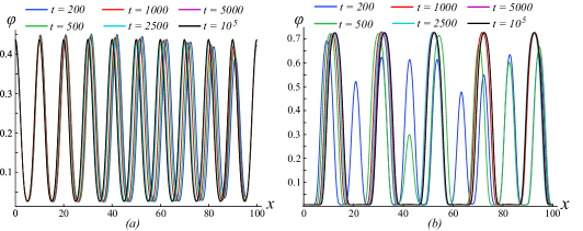
Figure 3: 1D concentration profile of component $\phi$ at various time. Parameters: $c_{A,0}=c_{B,0}=0.25$, (a): $\beta=0.1$, (b): $\beta=0.01$.

Furthermore, the impact of the dissociation constant on the evolution of the concentration is elucidated in Fig. 4. The concentration profiles depict the profound influence of the varying dissociation constant on the dynamics of phase separation, underscoring its critical role in this process. The regular arrangement of the concentration peaks is quickly established. Notably, an increase in the value of $\beta$ leads to higher frequencies and smaller amplitudes of concentration waves.

Similarly, Fig. 5 illustrates the one-dimensional volume fraction profile of the component $C$ for different initial concentrations at two different dissociation constant values. In Fig.5(a), the dynamics of the peak-forming patterns are observed for $\beta=0.1$. It is evident that increasing the initial concentrations of the reacting components results in longer wavelengths and greater amplitude. In contrast, in Fig. 5(b) as the dissociation constant $\beta$ decreases, the system undergoes a change in dynamics. For small initial concentrations, only a few peaks with extensive trough areas are observed. However, as concentration increases, the trough regions decrease in size, leading to the formation of mesa patterns, characterized by increased crest areas.

A comparative analysis of the results allows us to draw conclusions regarding the influence of the dissociation constant on the concentration patterns. Specifically, for a larger dissociation constant ($\beta=0.1$), concentration peaks exhibit regular and rapid establishment. On the contrary, for lower values of $\beta$ ($\beta=0.01$), a coarsening of the phase region is observed.

The concentration profiles obtained in Fig. 4 and Fig. 5 demonstrate stationary behavior, since they remain unchanged throughout the calculation period from $t=10^{4}$ up to $t=5\cdot 10^{5}$. The wavelengths of the regular concentration profiles correspond approximately to the wave vector at the maxima $K_{max}$ of the dispersion relation, as shown in Fig. 2. These one-dimensional calculations provide valuable insights into how the choice of model parameters can influence the phase separation process in higher dimensions, highlighting important trends.

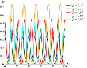
Figure 4: 1D concentration profile of component $C$ at various $\beta$ and $t=10^{5}$, $c_{A,0}=c_{B,0}=0.25$

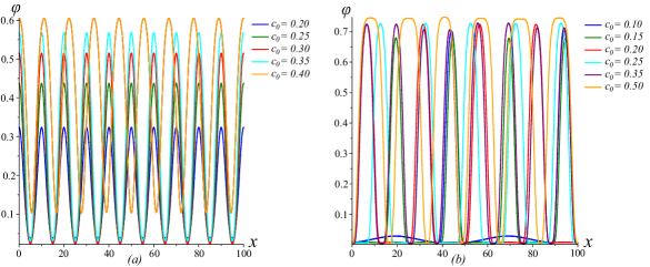
Figure 5: 1D concentration profile $\phi$ at various initial concentrations $c_{A,0}=c_{B,0}=c_{0}$ at $t=10^{5}$, (a): $\beta=0.1$, (b): $\beta=0.01$.

5.2 2D simulations

This section examines 2D simulations of concentration profiles. Previous studies have focused mainly on using 2D models to investigate the development of diatom structures and pattern formation. This choice is motivated by the computational ease and flat shape of the silica deposition vesicle in diatoms. In this part, we present the findings of 2D simulations that demonstrate steady state patterns in the volume fraction of the component $C$. Initially, we simulate the system of equations (9)-(11) on a square domain with periodic boundary conditions. As in the 1D results, we fixed the domain size to be 100, the diffusion coefficients to be $D_{A}=100$ and $D_{B}=1000$, and the phosphorylation rate $\alpha$ to be 10. The calculation period in simulations is $t=5\cdot 10^{5}$.

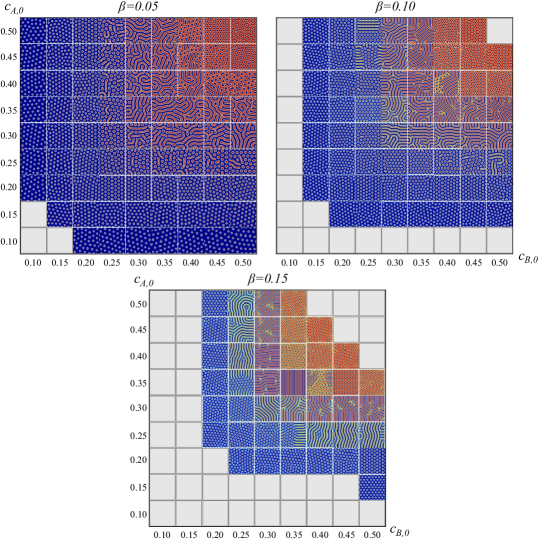
Figure 6: Concentration profile at fixed dissociation rate , the red color corresponds to the organic-rich phase. For the maximum concentration see Fig. S2.

In the first set of simulations, we maintained a constant dissociation rate $\beta$ (set to a specific value e.g. for each illustrated data set in Fig. 6) for simplicity while varying the initial concentrations of the components $A$ and $B$. This was done to observe how these concentrations affect the formation of patterns. The results for different values of the dissociation rate $\beta$ are illustrated in Fig. 6, where the organic-rich phase is represented in red. The simulations demonstrate that the system exhibits five different types of pattern, as illustrated in the schematic pattern diagram and particular cases for given values of $\beta$ in Fig. 7. Among these types, three are considered as the main types, while the remaining two are ’transitional’ or ’mixed’ types.

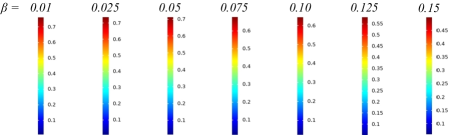
Figure S2: color bars: variation of concentration $\phi$ with dissociation rate $\beta$

The maximum concentration varies with the parameter $\beta$, see Fig. S2.

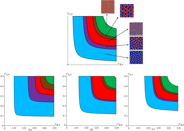
Figure 7: Pattern diagram at fixed values of dissociation rate and and particular cases for given values: $(a)$ $\beta=0.05$, $(b)$ $\beta=0.10$ and $(c)$ $\beta=0.15$.

The first type of patterns, shown in blue in Fig. 6, occurs when the initial concentrations of phosphate ions and organic molecules are low. These patterns exhibit a regular structure and consist of aggregates of organic "droplets" that are uniformly sized. The arrangement of these droplets is hexagonal or nearly hexagonal.

The second category of patterns, represented by the violet color in the pattern diagram, emerges when the initial concentrations are increased. In this case, the organic phase expands, leading to elongation of certain droplets and the formation of alignments. These patterns exhibit a combination of alignment structures and droplets.

As the concentration further increases, distinct patterns appear in the form of lamellar (labyrinth-like) structures. These patterns indicate that there is no dominant phase present. In Figure 6, these patterns are represented by the red color. It should be noted that these stripes remain stationary despite their irregular structure.

When initial concentrations are high, a regular structure of a dense network of organic-rich phase components $C$ with circular pores of organic-poor phase forms. These patterns are represented by the green color in the diagram.

Finally, patterns characterized by a dense network consisting of a combination of stripes and pores of the organic-dilute phase are shown in brown in Fig. 6.

The influence of periodic boundary conditions on the observed patterns in our simulations is an important factor to consider, which arises from the limited size of our simulation cell. To minimize the artificial effects caused by this limitation, we conducted the simulations with periodic boundary conditions. This approach was chosen as a means to optimize simulations for constrained geometries using a phase separation mechanism.

In diatoms, the aggregation of organic material occurs within the Silica Deposition Vesicle (SDV). It is worth noting that the SDV’s confinement is significantly larger than the pores observed in diatom valves. Hence, it is reasonable to focus on a small section of the SDV and assume periodic boundary conditions for our calculations. This decision is in line with the practical limitations of diatom structures.

Moreover, experimental evidence indicates that the type of soluble silica, together with the biomolecules involved in silica precipitation, can significantly influence the resulting silica morphology under varying conditions [25, 36, 4].

The region in which spinodal decomposition occurs is delineated by the lines determined by equation (26). By computing the equilibrium free energy $\phi$ using the equation (14) for various combinations of parameters and plotting it against the corresponding pattern types, we observe that each pattern type emerges within a specific range of $\phi_{e}$ values. This correlation is illustrated in Fig. 8.

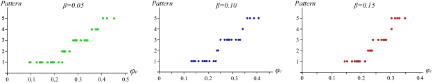
Figure 8: Pattern’s type vs equilibrium free energy $\phi_{e}$ at precise values of $\beta$.

In the second set of simulations, we set the initial concentrations of phosphate ions and organic molecules to be equal, denoting $c_{A,0}=c_{B,0}=c_{0}$. By varying $c_{0}$ and $\beta$, we obtained two-dimensional profiles of the concentration of the component $C$, presented in Fig. 9. This study provides valuable insights into the impact of the backward reaction and initial concentrations on pattern formation. The resulting pattern diagram is shown in Fig. 9. Similarly to the previous set of simulations, we observe that the system exhibits five types of patterns.

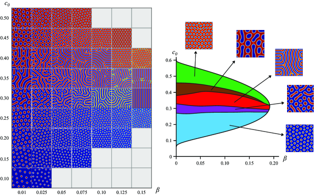
Figure 9: Stationary patterns of 2D concentration of component $C$ up to very large computation time ($c_{A,0}=c_{B,0}=c_{0}$), the red color corresponds to the organic-rich phase (displayed on the left, for the maximum concentration see Fig. S2) and Pattern diagram: the grey color indicates a scenario where no pattern formation (shown on the right).

Analyzing the results of the two sets of simulations provides valuable insights into the influence of initial concentrations and reverse reaction on pattern formation. An in-depth analysis of the patterns obtained in Fig.6, for the case where the dissociation rate remains constant, reveals that the parameter $\beta$, which represents the rate of the backward reaction, plays a key role in determining the wavelength of the resulting two-dimensional concentration profiles of the component $C$. This suggests that for a given value of $\beta$, the minimum distance between two nearest droplets in the droplet patterns, between the midlines for lamellar patterns or neighboring pores in the dense network of the organic-rich phase remains approximately constant regardless of changes in initial concentrations $c_{A,0}$ and $c_{B,0}$.

Moreover, the variations in $\beta$ shown in Fig. 9 cause either a refinement or coarsening of the structure, depending on whether the dissociation rate increases or decreases, respectively. Specifically, for droplet patterns, this correlation is illustrated in Fig. 10(a). Increasing in $\beta$ results in a shorter wavelength pattern. This relationship is illustrated in Fig. 10(b), which graphically represents the average wavelength alongside its standard deviation. For fixed initial concentration the size of the droplets, pores and lamellar structures scale with the pattern wavelength so that decreasing $\beta$ essentially causes the whole pattern to expand, specially see Fig. 10(c).

It is important to note that the similarities between the observed variations in $\beta$ and their impact on the wavelength are consistent with the findings derived from the stability analysis’s dispersion relation (19) and the outcomes of 1D simulations conducted for the examined equation system. This relationship is clearly depicted in Fig. 2$(c)$ and the 1D simulations displayed in Fig. 4. The agreement in findings across these different analytical approaches emphasizes the reliability and coherence of our conclusions regarding the complex dynamics of the system under the influence of different dissociation rates.

After a detailed examination of the results obtained from both sets of simulations, a significant finding becomes apparent: the morphology of the patterns is related to the initial concentrations of both reactants, $c_{A,0}$ and $c_{B,0}$. The transition from one type of pattern to another occurs only with a sufficient change in the concentrations of both reacting components. The size of the phase-separated components is largely influenced by the initial concentrations of phosphate ions and organic molecules. When the dissociation rate remains constant, an increase in the concentration of either of the reacting components leads to the enlargement of the area occupied by the organic-rich phase. This is illustrated in Fig. 10$(a)$. The expansion of the organic-rich area, in turn, helps in the creation of various organic-rich networks that exhibit unique characteristics specific to each mentioned pattern. It is important to mention that the rate at which the organic-rich phase grows is higher when the initial concentration of phosphate ions increases, compared to the same increase in the concentration of organic molecules. Based on these observations, we can identify a way to adjust the scale of patterns, as shown in Figure 10$(c)$ for the droplet pattern.

To study the formation of patterns in the growing valve [19, 9] and the hierarchical pore structure of diatoms [45, 44], where larger pores act as confinements for the formation of smaller pores, a series of simulations were conducted using a circular geometry. To evaluate the stability and applicability of our results, we carried out these simulations in a circular simulation domain with zero-flux boundary conditions. The resulting patterns are shown in Fig. 11. The patterns obtained remain stationary throughout the simulation time from $t=2\cdot 10^{4}$ of $t=5\cdot 10^{5}$. However, it is important to note that there is a possibility of changes occurring at extremely long times.

It is worth mentioning that the patterns obtained within the circular simulation cell closely resemble those derived from the previous sets of simulations, as shown in Fig. 6,9, when the model parameters have the same values. The uniformity across various geometries not only enhances the reliability of our findings but also emphasizes the inherent characteristics of the observed patterns, which are influenced by the dynamics governed by the specified model parameters.

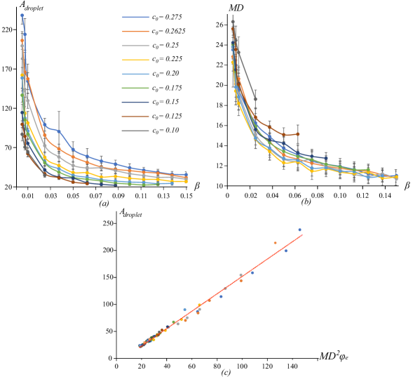
Figure 10: (a) Average size of organic droplets depending on dissociation rate for various initial concentration. (b) Minimum distance between two closest neighboring droplets. (c) Pattern scaling: dependence of area of droplet on pattern wavelength and equilibrium volume fraction.

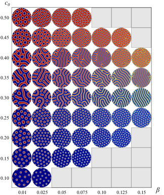
Figure 11: Circular stationary patterns: Concentration profiles of component $C$ within a circular boundary ($c_{A,0}=c_{B,0}=c_{0}$). For the maximum concentration, refer to Fig. S2.

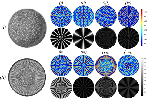
Figure 12: Experimental (on the left) and simulated (on the right) structures of centric diatoms. (I) Coscinodiscus, (II) Stephanodiscus medius. During the simulations, the shared parameters were $\beta=0.15$, $c_{A,0}=0.2$, and $c_{B,0}=0.25$. Simulated images (top) and the corresponding pre-patterning fields $h$ that were used in the simulations: (i) $0.5cos^{10}(8\theta)$, (ii) $0.5(1+10sin^{2}(3\theta))^{-1}$, (iii) $0.09cos^{2}(26\theta)$, (iv) $0.05cos^{6}(0.12\pi\sqrt{x^{2}+y^{2}})+0.08cos^{8}(8\theta)$, (v) $0.4cos^{2}(18\theta)$, (vi) $0.08cos^{8}(8\theta)$, (vii) $0.18cos^{2}(26\theta)$, (viii) $0.1cos^{2}(4\theta)$. Permission for experimental images has been requested [37, 8].

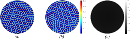
Figure 13: Effect of Prepatterning Field: (a) Pattern on a computational domain with zero-flux boundary conditions, (b) Pattern on a computational domain with corresponding prepatterning field on (c), which is defined by $h=0.5$ for $R\in[99.75,100]$ or $h=0$ otherwise. Shared parameters: $\beta=0.1125$, $c_{A,0}=c_{B,0}=0.225$.

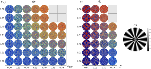
Figure 14: Circular stationary patterns: Concentration profiles of component $C$ within a circular boundary for $(a)$$\beta=0.15$ and $(b)$ $c_{A,0}=c_{B,0}=c_{0}$ for prepatterning field $h=0.15sin^{4}(6\theta)$ on $(c)$. For the maximum concentration see Fig. S2.

In my current role, my research work is concerned to mathematical modelling of diatom frustule morphogenesis, a multiphysics problem that combines chemical reactions, diffusion and liquid-liquid phase separation.

This comprehensive study greatly enhances our understanding of the complex dynamics that govern the formation of patterns in the system under study. The observed patterns remain stationary during the simulation for times after $t=2\cdot 10^{4}$ and act as a template that guides silica deposition.

6 Prepatterning

In this section, our goal is to examine the impact of "prepatterning" caused by the existence of silica costae in the base layer on the liquid-liquid phase separation process. We extend the research conducted by Lenoci et al.[26] to investigate how prepatterns, like costae that preexist the pores, impact the final patterns. Notably, in the work of Lenoci and Camp the final patterns were not stationary and were not coupled with chemical reactions.

In summary, my research interests are driven by a passion for understanding the fundamental principles governing complex biological and chemical phenomena through interdisciplinary research and data-driven modelling approaches. I am eager to bring my expertise and interdisciplinary perspective to your research group at and contribute to the field of collective cell behaviour and way for innovative solutions to pressing biomedical challenges.

To simulate the presence of silica costae, a characteristic feature of diatoms, during the early stages of frustule formation, we introduce an additional term $h$ into the equation of free energy (5). This term represents the local field generated by the preexisting silica ribs, contributing to the formation of the prepatterning structure. Thus, the modified free energy equation (5) that governs the thermodynamic state of the phase-separating component becomes the following:

$$F[\phi]=\int\left(f(\phi)+\cfrac{\kappa}{2}(\nabla\phi)^{2}+h\phi\right)$$ (27)

The prepatterning field is designed to mimic the morphology of costae observed in real diatoms. We focus on centric diatoms with circular valves, which can be classified into two types based on valve morphology. The first type includes diatoms whose valve face exhibits a single common morphology. In this type, the areolae, regularly repeated pores, may be hexagonal, radiate from a central annulus, a hyaline ring, or be arranged in radial rows. Examples include Actinocyclus, Eupodiscus, and others. The second type comprises diatoms with valves divided into two parts (central and marginal areas), each with distinct morphologies, e.g. central areolae surrounded by radiating striae. Examples include Brevisira, Stephanodiscus, and others.

Based on this division and observation, we select appropriate functions for the prepatterning field to correspond to the shape of the costae. In Fig. 12, we present experimental images of selected diatoms from two distinct classes alongside variety of simulated structures produced by employing different prepatterning fields, illustrating the variety of attainable patterns and highlighting how the prepatterning field can accurately represent the unique characteristics of diatom morphology.

In addition, prepatterning fields can be used to solve numerical problems encountered during simulations. During our computations, we noticed the formation of organic half-droplets at the boundaries of our numerical domain. To circumvent this problem and ensure that all droplets remain inside the simulation cell, we applied a thin layer of prepattern field to the boundary. Illustrated in Fig. 13(a) is the numerical domain with zero-flux boundary conditions, where half-droplets are visible at the boundaries. In Fig. 13 (b,c), the same domain but with the inclusion of prepatterning field at the boundary, resulting in all droplets being held within the cell. Importantly, all computations were performed using the same parameters, underscoring the effectiveness of the prepatterning field in eliminating numerical anomalies while maintaining the validity of the simulation outcomes.

Simulations with different initial concentrations and dissociation rates were conducted similarly to the previous sections. Results presented in Fig. 14 elucidate how variations in initial concentrations and dissociation rate affect the resulting patterns in the presence of prepatterning induced by silica costae.

Overall, incorporating the prepatterning field into our simulations not only enables us to precisely mimic the morphology of diatoms but also enhances the precision and robustness of our computational models by mitigating boundary effects and ensuring consistency with experimental observations.

7 Discussions

Our investigation into the role of phosphate ions and organic molecules in diatom silica structure formation has provided valuable insights into the mechanisms driving pattern formation. By exploring the hypothesis of organic template-driven silica morphogenesis, our study focused on the aggregation of organic molecules through a phase separation model, supported by in vitro experiments highlighting the catalytic role of organic components.

The approach used in this paper couples the phase separation process with a chemical reaction, allowing the phase-separating component to dissociate into two constituents. Unlike previous studies [5, 26], our work involved detailed analysis to elucidate the conditions necessary for pattern formation and to understand how model parameters and prepatterning field affect pattern morphology and transitions between different types of patterns.

The study in [15] shows that the chemical reaction suppresses spinodal decomposition, limiting the ongoing coarsening of the phase domains during phase separation. Building on the framework presented by Bobeth et al. in [5], which couples phase separation with chemical reactions, the objective of this article was to explore the effects of model parameters on pattern formation. We provided valuable insights into the interplay of initial concentrations and dissociation coefficients that govern phase separation. Through stability analysis, we established conditions for pattern formation and assessed how initial concentrations and dissociation rate affect the dispersion relation. Our numerical simulations identified five distinct pattern types and emphasised the role of initial concentrations and of the reverse reaction rate in the formation of these patterns. Experimental evidence indicated that the type of soluble silica and biomolecules significantly influence silica morphology under different conditions [4, 25, 36]. Consequently, our findings provide a robust framework for integration of these insights into more advanced models and in vitro experiments designed to clarify these morphological variations in silica. In our work, we demonstrated that the pattern morphology depends on the initial concentrations of organic molecules and phosphate ions. We observed that transitioning between pattern types requires significant changes in the concentrations of both reacting constituents. Increasing the concentration of any reactant enlarges the region dominated by the organic-rich phase, facilitating the formation of diverse organic-rich networks, each exhibiting distinct characteristics reflective of their pattern types.

In [26], phase separation was induced by an additional local field due to the existing silica costae in the base layer, leading to the formation of various two-dimensional patterns that closely resembled the observed valve structures. However, in [26], phase separation is not coupled with chemical reaction and diffusion, and therefore there is a complete coarsening of organic-rich phase regions [15]. In our study, we integrate the prepatterning field into the reaction-diffusion model coupled with phase separation to mimic the presence of costae, contributing to pore formation. Our results show that diatom valve pore structures can be qualitatively mimicked by a liquid-liquid phase separation model combined with a chemical reaction. Although accurately reproducing observed diatom structures would necessitate a more complex model, our research indicates that features such as costae and pores can be produced in silico as a negative imprint of the phase-separated organic template.

Although our computer simulations have provided valuable insights, it is important to recognise their limitations. A more sophisticated modelling approach is needed, particularly to address the complexities of nonlinear diffusion and phase separation dynamics, as well as to account for the electrostatic interactions between organic droplets and silica ribs and the growth of the SDVs during valve development. As the diameter of the SDVs increases, the silica ribs grow radially, necessitating an extension of our model to include the growing domain, which has an interesting effect on pattern formation (see e.g., [6, 7, 22]). This should also incorporate a recent study on branching morphogenesis [2] and costae growth. Furthermore, comparing our work with mass-conserving reaction-diffusion systems (see, e.g., [42]) holds considerable interest and can provide valuable insights into the underlying mechanisms.

By integrating theoretical modelling with in vitro experimental validation, we can enhance our understanding of these captivating biological phenomena and potentially apply them in various fields such as biomimetics and materials science. Experimental studies are crucial for the precise calibration of specific model parameters, while the insights gained from our simulations may provide a solid foundation for future in vitro methodologies. These approaches could strategically adjust critical factors such as the pH level and the concentration of reacting constituents, thereby controlling the biosilica formation process.

Furthermore, our approach holds promise for studies aimed at the creation of artificial SDV under in vitro conditions. The modelling performed within this framework can further facilitate the modelling of the silica stuctures, in which the arrangement of organic aggregates acts as a template for silica formation following the addition of monosilicic acid to the system.

8 Acknowledgments

The work was funded by a Leverhulme Trust Research Project Grant (RPG-2021-181). We gratefully acknowledge Dr. Philip Pearce for help with COMSOL.

Figure S1: Influence of Flory-Huggins interaction parameter on spinodal decomposition for $N=10$.

Appendix S1 Numerical integration of PDEs

To numerically integrate the system of nonlinear partial differential equations (9)-(11), we employed the CFD Module in Comsol Multiphysics. Using in a nonlinear time-dependent solver the backward Euler method, we sought to capture the dynamics of the system accurately. The boundary conditions and parameters utilized in the simulations are detailed in the main text.

However, simulations of the initial system (9)-(11) proved to be computationally intensive and slow, particularly at lower values of $\beta$. To accelerate the simulations without compromising accuracy,we adopted an approximate 4D system approach. This approximated system, outlined below, yields solutions equivalent to those of the initial system, but with significantly improved computational speed:

$$\cfrac{\partial\widehat{c}_{A}}{\partial\widehat{t}}=\widehat{\nabla}\cdot\widehat{D}_{A}\widehat{\nabla}\widehat{c}_{A}-\widehat{\alpha}\widehat{c}_{A}\widehat{c}_{B}+\widehat{\beta}\phi$$ (28)

$$\cfrac{\partial\widehat{c}_{B}}{\partial\widehat{t}}=\widehat{\nabla}\cdot\widehat{D}_{B}\widehat{\nabla}\widehat{c}_{B}-\widehat{\alpha}\widehat{c}_{A}\widehat{c}_{B}+\widehat{\beta}\phi$$ (29)

$$\cfrac{\partial\phi}{\partial\widehat{t}}=\widehat{\nabla}^{2}\mu+\widehat{\alpha}\widehat{c}_{A}\widehat{c}_{B}-\widehat{\beta}\phi$$ (30)

$$\epsilon\cfrac{\partial\mu}{\partial\widehat{t}}+\mu=\widehat{f}^{\prime}(\phi)-\widehat{\nabla}^{2}\phi,$$ (31)

where $\epsilon\ll 1$, in our calculations we put $\epsilon=10^{-4}$. The solutions derived from the approximated 4D system are closely aligned with those of the original system, but the solver shows significantly improved efficiency. This method enables an effective investigation of the system’s dynamics and behavior with reduced computational demands.

References

- [1] A. Alverson. The air you’re breathing? a diatom made that. Live Science, 2014.
- [2] I. Babenko, N. Kröger, and B. M. Friedrich. Mechanism of branching morphogenesis inspired by diatom silica formation. Proceedings of the National Academy of Sciences, 121(10):e2309518121, 2024.
- [3] A.-S. Benoiston, F. M. Ibarbalz, L. Bittner, L. Guidi, O. Jahn, S. Dutkiewicz, and C. Bowler. The evolution of diatoms and their biogeochemical functions. Philosophical Transactions of the Royal Society B: Biological Sciences, 372(1728):20160397, 2017.
- [4] A. Bernecker, R. Wieneke, R. Riedel, M. Seibt, A. Geyer, and C. Steinem. Tailored synthetic polyamines for controlled biomimetic silica formation. Journal of the American Chemical Society, 132(3):1023–1031, 2010.
- [5] M. Bobeth, A. Dianat, R. Gutierrez, D. Werner, H. Yang, H. Eckert, and G. Cuniberti. Continuum modelling of structure formation of biosilica patterns in diatoms. BMC Materials, 2:1–11, 2020.
- [6] E. J. Crampin, E. A. Gaffney, and P. K. Maini. Reaction and diffusion on growing domains: scenarios for robust pattern formation. Bulletin of mathematical biology, 61(6):1093–1120, 1999.
- [7] E. J. Crampin, W. W. Hackborn, and P. K. Maini. Pattern formation in reaction-diffusion models with nonuniform domain growth. Bulletin of mathematical biology, 64:747–769, 2002.
- [8] B. D and E. M. Stephanodiscus medius. in diatoms of north america, 2015. https://diatoms.org/species/stephanodiscus_medius.
- [9] D. de Haan, L. Aram, H. Peled-Zehavi, Y. Addadi, O. Ben-Joseph, R. Rotkopf, N. Elad, K. Rechav, and A. Gal. Exocytosis of the silicified cell wall of diatoms involves extensive membrane disintegration. Nature communications, 14(1):480, 2023.
- [10] L. De Stefano, I. Rea, I. Rendina, M. De Stefano, and L. Moretti. Lensless light focusing with the centric marine diatom coscinodiscus walesii. Optics Express, 15(26):18082–18088, 2007.
- [11] M. De Stefano, L. De Stefano, and R. Congestri. Functional morphology of micro-and nanostructures in two distinct diatom frustules. Superlattices and Microstructures, 46(1-2):64–68, 2009.
- [12] E. De Tommasi, L. De Stefano, I. Rea, L. Moretti, M. De Stefano, and I. Rendina. Light micro-lensing effect in biosilica shells of diatoms microalgae. In Micro-Optics 2008, volume 6992, pages 124–128. SPIE, 2008.
- [13] J. Delasoie and F. Zobi. Natural diatom biosilica as microshuttles in drug delivery systems. pharmaceutics, 11, 537, 2019.
- [14] A. P. Garcia and M. J. Buehler. Bioinspired nanoporous silicon provides great toughness at great deformability. Computational Materials Science, 48(2):303–309, 2010.
- [15] S. C. Glotzer, E. A. Di Marzio, and M. Muthukumar. Reaction-controlled morphology of phase-separating mixtures. Physical review letters, 74(11):2034, 1995.
- [16] R. Gordon and R. W. Drum. The chemical basis of diatom morphogenesis. In International review of cytology, volume 150, pages 243–372. Elsevier, 1994.
- [17] M. S. Hale and J. G. Mitchell. Functional morphology of diatom frustule microstructures: hydrodynamic control of brownian particle diffusion and advection. Aquatic Microbial Ecology, 24(3):287–295, 2001.
- [18] C. E. Hamm, R. Merkel, O. Springer, P. Jurkojc, C. Maier, K. Prechtel, and V. Smetacek. Architecture and material properties of diatom shells provide effective mechanical protection. Nature, 421(6925):841–843, 2003.
- [19] C. Heintze, I. Babenko, J. Zackova Suchanova, A. Skeffington, B. M. Friedrich, and N. Kröger. The molecular basis for pore pattern morphogenesis in diatom silica. Proceedings of the National Academy of Sciences, 119(49):e2211549119, 2022.
- [20] C. Jeffryes, R. Solanki, Y. Rangineni, W. Wang, C.-h. Chang, and G. L. Rorrer. Electroluminescence and photoluminescence from nanostructured diatom frustules containing metabolically inserted germanium. Advanced Materials, 20(13):2633–2637, 2008.
- [21] J. D. Joannopoulos, P. R. Villeneuve, and S. Fan. Photonic crystals. Solid State Communications, 102(2-3):165–173, 1997.
- [22] A. L. Krause, M. A. Ellis, and R. A. Van Gorder. Influence of curvature, growth, and anisotropy on the evolution of turing patterns on growing manifolds. Bulletin of mathematical biology, 81:759–799, 2019.
- [23] N. Kroger, S. Lorenz, E. Brunner, and M. Sumper. Self-assembly of highly phosphorylated silaffins and their function in biosilica morphogenesis. Science, 298(5593):584–586, 2002.
- [24] N. Kröger and K. H. Sandhage. From diatom biomolecules to bioinspired syntheses of silica-and titania-based materials. Mrs Bulletin, 35(2):122–126, 2010.
- [25] C. C. Lechner and C. F. Becker. Silaffins in silica biomineralization and biomimetic silica precipitation. Marine drugs, 13(8):5297–5333, 2015.
- [26] L. Lenoci and P. J. Camp. Self-assembly of peptide scaffolds in biosilica formation: computer simulations of a coarse-grained model. Journal of the American Chemical Society, 128(31):10111–10117, 2006.
- [27] D. Losic, J. G. Mitchell, and N. H. Voelcker. Diatomaceous lessons in nanotechnology and advanced materials. Advanced Materials, 21(29):2947–2958, 2009.
- [28] A. J. Milligan and F. M. Morel. A proton buffering role for silica in diatoms. Science, 297(5588):1848–1850, 2002.
- [29] D. Pawolski, C. Heintze, I. Mey, C. Steinem, and N. Kröger. Reconstituting the formation of hierarchically porous silica patterns using diatom biomolecules. Journal of Structural Biology, 204(1):64–74, 2018.
- [30] S. Phogat, A. Saxena, N. Kapoor, C. Aggarwal, and A. Tiwari. Diatom mediated smart drug delivery system. Journal of Drug Delivery Science and Technology, 63:102433, 2021.
- [31] N. Rabiee, M. Khatami, G. Jamalipour Soufi, Y. Fatahi, S. Iravani, and R. S. Varma. Diatoms with invaluable applications in nanotechnology, biotechnology, and biomedicine: recent advances. ACS biomaterials science & engineering, 7(7):3053–3068, 2021.
- [32] I. Rea and L. De Stefano. Recent advances on diatom-based biosensors. Sensors, 19(23):5208, 2019.
- [33] F. E. Round, R. M. Crawford, and D. G. Mann. Diatoms: biology and morphology of the genera. Cambridge university press, 1990.
- [34] A. M. M. Schmid and D. Schulz. Wall morphogenesis in diatoms: deposition of silica by cytoplasmic vesicles. Protoplasma, 100:267–288, 1979.
- [35] M. Sumper. A phase separation model for the nanopatterning of diatom biosilica. Science, 295(5564):2430–2433, 2002.
- [36] M. Sumper and E. Brunner. Learning from diatoms: Nature’s tools for the production of nanostructured silica. Advanced Functional Materials, 16(1):17–26, 2006.
- [37] F. T. Coscinodiscus. in diatoms of north america, 2022. https://diatoms.org/genera/coscinodiscu.
- [38] P. Tréguer, C. Bowler, B. Moriceau, S. Dutkiewicz, M. Gehlen, O. Aumont, L. Bittner, R. Dugdale, Z. Finkel, D. Iudicone, et al. Influence of diatom diversity on the ocean biological carbon pump. Nature Geoscience, 11(1):27–37, 2018.
- [39] B. Volcani. Cell wall formation in diatoms: morphogenesis and biochemistry. In Silicon and siliceous structures in biological systems, pages 157–200. Springer, 1981.
- [40] J.-K. Wang and M. Seibert. Prospects for commercial production of diatoms. Biotechnology for Biofuels, 10:1–13, 2017.
- [41] Y. Watanabe and D. O. Hall. Photosynthetic co2 conversion technologies using a photobioreactor incorporating microalgae-energy and material balances. Energy conversion and management, 37(6-8):1321–1326, 1996.
- [42] H. Weyer, F. Brauns, and E. Frey. Coarsening and wavelength selection far from equilibrium: a unifying framework based on singular perturbation theory. Physical Review E, 108(6):064202, 2023.
- [43] R. Wieneke, A. Bernecker, R. Riedel, M. Sumper, C. Steinem, and A. Geyer. Silica precipitation with synthetic silaffin peptides. Organic & biomolecular chemistry, 9(15):5482–5486, 2011.
- [44] L. Willis, E. Cox, and T. Duke. A simple probabilistic model of submicroscopic diatom morphogenesis. Journal of the Royal Society Interface, 10(83):20130067, 2013.
- [45] L. Willis, K. M. Page, D. S. Broomhead, and E. J. Cox. Discrete free-boundary reaction-diffusion model of diatom pore occlusions. Plant Ecology and Evolution, 143(3):297–306, 2010.
- [46] F. Zobi. Diatom biosilica in targeted drug delivery and biosensing applications: Recent studies. In Micro, volume 2, pages 342–360. MDPI, 2022.