A randomly generated Majorana neutrino mass matrix using Adaptive Monte Carlo method

Abstract

A randomly generated complex symmetric matrix using Adaptive Monte Carlo method, is taken as a general form of Majorana neutrino mass matrix, which is diagonalized by the use of eigenvectors. We extract all the neutrino oscillation parameters i.e. two mass-squared differences ($\Delta m_{21}^{2}$ and $\Delta m_{32}^{2}$ ), three mixing angles ($\theta_{12}$, $\theta_{13}$, $\theta_{23}$) and three phases i.e. one Dirac CP violating phase ($\delta_{CP}$) and two Majorana phases ($\alpha$ and $\beta$). The charge-parity (CP) violating phases are extracted from the mixing matrix constructed with the eigenvectors of the Hermitian matrix formed by the complex symmetric matrix. All the neutrino oscillation parameters within 3$\sigma$ bound are allowed in both normal hierarchy (NH) and inverted hierarchy (IH) consistent with the latest Planck cosmological upper bound, $\sum|m_{i}|<0.12$ eV. This latest cosmological upper bound is allowed only in three cases of zero texture for $m_{11}=0$; $m_{11},m_{12}=0$ and $m_{11},m_{13}=0$ in normal hierarchy whereas none of zero texture is allowed in inverted hierarchy. We also study effective neutrino masses $m_{\beta}$ in tritium beta decay and $m_{\beta\beta}$ in neutrinoless double beta decay.

Keywords :Majorana neutrino mass matrix, Adaptive Monte Carlo method, Normal and Inverted hierarchical mass models, Zero-texture

1 Introduction

The present neutrino oscillation data confirms that neutrinos have very tiny but non-zero masses. These tiny masses of neutrinos are elegantly explained by the celebrated seesaw mechanism[1, 2]. Texture of neutrino mass matrices, is one of the major issues in neutrino physics. Attempts have been made[3, 4, 5, 6] to construct possible neutrino mass matrices, including zero-texture models. However, the ambiguity in the choice of the correct form of this texture, is not yet resolved. With the hope to discriminate among these theoretically predicted possible textures, we adopt a different approach that may give some hints on the correct structure of the Majorana neutrino mass matrix consistent with the presently available neutrino oscillation data. One such approach is the Adaptive Monte Carlo method for randomly generating the complex Majorana neutrino mass matrix[7, 8].

A Majorana maas matrix, $m_{\nu}$ can be constructed by using a set of six real numbers as well as a set of six complex numbers. A set of real numbers can form only a symmetric Majorana mass matrix for charge-parity (CP) conserving case with Dirac phase, $\delta_{CP}=0$. This Majorana neutrino mass matrix is diagonalized the use of the standard mixing matrix, $U$ as follows,

$$M_{diag}=diag(m_{1},m_{2},m_{3})=U^{T}m_{\nu}U$$ (1)

For CP non-conserving case with $\delta_{CP}\neq 0$, a 3$\times$3 complex symmetric matrix is taken as a general form of Majorana mass matrix, $m_{\nu}$. Using complex symmetric mass matrix, one can construct a Hermitian matrix $h$ as $h=m_{\nu}m_{\nu}^{{\dagger}}$, which is digonalized as[9]

$$U^{{\dagger}}hU=diag(m_{1}^{2},m_{2}^{2},m_{3}^{2})=D$$ (2)

where the $U$ is mixing matrix constructed with the eigenvectors of $h$ and $m_{i}^{2}$ (i=1,2,3) are the mass-squared eigenvalues.

The general form of Majorana neutrino mass matrix has the following structure:

$$m_{\nu}=\left(\begin{array}[]{ccc}a&b&c\\ b&d&e\\ c&e&f\end{array}\right)=\left(\begin{array}[]{ccc}m_{11}e^{i\phi_{11}}&m_{12}e^{i\phi_{12}}&m_{13}e^{i\phi_{13}}\\ m_{12}e^{i\phi_{12}}&m_{22}e^{i\phi_{22}}&m_{23}e^{i\phi_{23}}\\ m_{13}e^{i\phi_{13}}&m_{23}e^{i\phi_{23}}&m_{33}e^{i\phi_{33}}\end{array}\right)$$ (3)

One of the major reasons for considering complex symmetric matrix is to extract the charge-parity (CP) violating one Dirac phase and two Majorana phases. A real symmetric matrix gives only real eigenvectors whereas a complex symmetric matrix gives complex eigenvectors. The elements of mixing matrix, $U$ constructed by eigenvectors, should also be complex numbers which lead to CP-violating phases. The general form of mixing matrix, $U$ takes the following form[10]

$$U=\left(\begin{array}[]{ccc}c_{13}c_{12}&c_{13}s_{12}&s_{13}e^{-i\delta_{CP}}\\ -c_{23}s_{12}-c_{12}s_{13}s_{23}e^{-i\delta_{CP}}&c_{12}c_{23}-s_{12}s_{13}s_{23}e^{-i\delta_{CP}}&c_{13}s_{23}\\ s_{12}s_{23}-c_{12}s_{13}c_{23}e^{-i\delta_{CP}}&-c_{12}s_{23}-c_{23}s_{13}s_{12}e^{-i\delta_{CP}}&c_{13}c_{23}\end{array}\right).P$$ (7)

where $s_{ij}=\sin\theta_{ij}$, $c_{ij}=\cos\theta_{ij}$ and $\delta_{CP}$=Dirac CP violating phase. The matrix $P=diag(1,e^{-i\alpha_{1}/2},e^{-i\alpha_{2}/2})$ has two Majorana CP phases $\alpha_{1}$ and $\alpha_{2}$. From the complex mixing matrix $U$ and $D$, we can extract all neutrino oscillation data including the Dirac and Majorana CP-violating phases by using the following relations[11]: $\Delta m_{21}^{2}=m_{2}^{2}-m_{1}^{2}$; $\Delta m_{32}^{2}=m_{3}^{2}-m_{2}^{2}$; $\tan\theta_{12}=\frac{|U_{e2}|}{|U_{e1}|}$; $\tan\theta_{23}=\frac{|U_{\mu 3}|}{|U_{\tau 3}|}$; $\sin\theta_{13}=|U_{e3}|$.

For one Dirac CP-phase[11],

$$J_{CP}=Im[U_{e1}U_{\mu 2}U_{e2}^{*}U_{\mu}^{*}]=s_{12}c_{12}s_{23}c_{23}c_{13}s_{13}\sin\delta_{CP}$$ (8)

For two Majorana phases[11],

$$I_{1}=Im[U_{e1}^{*}U_{e2}]=c_{12}c_{13}^{2}s_{12}\sin(\frac{\alpha}{2})$$ (9)

$$I_{2}=Im[U_{e1}^{*}U_{e3}]=c_{12}c_{13}s_{13}\sin(\frac{\beta}{2}-\delta)$$ (10)

where $J_{CP}$ is the Jarlskog rephasing invariant quantity that measures the magnitude of Dirac CP violatrion, and $I_{1}$ and $I_{2}$ are other two invariant quantities that measure the magnitude of Majorana CP violation.

The present work is an attempt to construct a possible Majorana neutrino mass structure that can give all neutrino oscillation data within 3$\sigma$ bound[12, 13, 14]. There are generally two popular approaches to restrict the form of neutrino mass matrices namely, “top-down approach” - where the neutrino oscillation parameters are predicted from a given neutrino mass matrix and “bottom-up approach”- where the existing neutrino oscillation data determine possible texture of the neutrino mass matrix. The first method“top-down approach” relies on theoretical models associated with some discrete symmetries like $S_{3},S_{4},A_{4},A_{5}$ etc[15, 16, 17] and the second method “bottom up approach” relies on the numerical analysis. We have used “bottom-up approach” to construct possible neutrino mass matrix numerically with the available oscillation data within 3$\sigma$ bound[12]. The presently available neutrino oscillation data includes two mass-squared difference i.e. solar mass-squared difference ($\Delta m_{21}^{2}$) and atmospheric mass-squared difference ($\Delta m_{32}^{2}$); three neutrino mixing angles i.e. solar mixing angle ($\theta_{12}$), reactor mixing angle ($\theta_{13}$) and atmospheric mixing angle ($\theta_{23}$) and one Dirac CP violating phase ($\delta_{CP}$) respectively.

In this present study, a general complex Majorana neutrino mass matrix constructed with random input parameters, is diagonalized to generate an eigen-system which in turn predicts neutrino oscillation parameters consistent with the presently available oscillation data. The latest Planck cosmological upper bound on the sum of three absolute neutrino mass eigenvalues, $\sum|m_{i}|<0.12$eV [18, 19] is used as a constraint in the numerical analysis. Some texture models[20, 21] are also possible to study numerically. One zero texture and two zero texture are studied in both normal hierarchy and inverted hierarchy within this latest cosmological bound.

The paper is organised as follows. In Section 2, we give a brief outline of Adaptive Monte Carlo Method for generating Majorana mass matrix. Section 3 is devoted to numerical analysis and results. In Section 4, we give a summary and discussion.

2 Adaptive Monte Carlo method for generating Majorana mass matrix

The Dirac CP-violating phase can not be extracted from the real symmetric mass matrix. In order to extract the Dirac CP violating phase, the mass matrix should be a complex one i.e. all the elements of mass matrix are taken in the form of complex number as given below

$$m_{\nu}=\left(\begin{array}[]{ccc}a_{1}+ia_{2}&b_{1}+ib_{2}&c_{1}+ic_{2}\\ b_{1}+ib_{2}&d_{1}+id_{2}&e_{1}+ie_{2}\\ c_{1}+ic_{2}&e_{1}+ie_{2}&f_{1}+if_{2}\end{array}\right)$$ (11)

To construct numerically such a complex symmetric matrix, twelve real numbers are required i.e. a set of six real numbers for real part $\{a_{1},b_{1},c_{1},d_{1},e_{1},f_{1}\}$ and another set of six real numbers for imaginary part $\{a_{2},b_{2},c_{2},d_{2},e_{2},f_{2}\}$. These twelve real numbers are randomly generated within a given range, which are allowed by the latest Planck cosmological upper bound, $\sum|m_{i}|<0.12$ eV. For a particular Majorana neutrino mass matrix, the extracted two mass-squared differences ($\Delta m_{21}^{2}$ and $\Delta m_{32}^{2}$) and all the elements of neutrino mixing matrix, $U_{PMNS}$, are compared with the observed experimental values given in Table 1[22, 23, 7]. The general structure of neutrino mixing matrix ($U_{PMNS}$) is given below:

$$U=U_{PMNS}=\left(\begin{array}[]{ccc}U_{e1}&U_{e2}&U_{e3}\\ U_{\mu 1}&U_{\mu 2}&U_{\mu 3}\\ U_{\tau 1}&U_{\tau 2}&U_{\tau 3}\end{array}\right)$$ (12)

where, $\tan\theta_{12}=\frac{|U_{e2}|}{|U_{e1|}}$, $\tan\theta_{23}=\frac{|U_{\mu 3}|}{|U_{\tau 3}|}$, $\sin\theta_{13}=|U_{e3}|$.

i	$x_{i}\ \ \ \ \ \ \ \ \ \ \ \ \ \ \ \ \ \ \ \ \ \ \ \$	$x_{i}^{cent}\ \ \ \ \ \ \ \ \ \ \ \ \$	$\sigma_{i}$
1	$\Delta m_{32}^{2}[eV^{2}]$	$2.51\times 10^{-3}$	$10^{-3}$
2	$\Delta m_{21}^{2}[eV^{2}]$	$7.42\times 10^{-5}$	$10^{-5}$
3	$|U_{e1}|$	0.835	0.045
4	$|U_{e2}|$	0.54	0.07
5	$|U_{e3}|$	0.148	0.1
6	$|U_{\mu 1}|$	0.355	0.165
7	$|U_{\mu 2}|$	0.575	0.155
8	$|U_{\mu 3}|$	0.7	0.12
9	$|U_{\tau 1}|$	0.365	0.165
10	$|U_{\tau 2}|$	0.59	0.15
11	$|U_{\tau 3}|$	0.685	0.125

Table 1: The best-fit absolute values of the neutrino mass-squared differences and the elements of $U_{PMNS}$ with the 3$\sigma$ uncertainties.

The rejection rule for a considered mass texture to be a possible solution of Eq. (11) is defined as

$$\frac{(x_{i}^{cent}-x_{i})^{2}}{\sigma_{i}^{2}}\leq\frac{1}{\alpha^{2}}$$ (13)

where, $x_{i}^{cent}$ and $x_{i}$ represent the experimentally observed best-fit values and the numerically observed values of neutrino oscillation parameters respectively, while $\sigma_{i}$ and $\alpha$ are respectively the 3$\sigma$ uncertainties and a parameter which is used for fixing the assumed error $\sigma_{i}$. In the present analysis, we put $\alpha=1$ so that the results are obtained within 3$\sigma$ confidence level. If the extracted values of oscillation parameters from the mass matrix, are found to lie within the range of 3$\sigma$ bound, then it is one of the possible solutions to the general mass matrix of Eq.(11). To perform the numerical fitting of the mass matrix, we are using the Adaptive Monte Carlo method[7, 8]. This method also enables us to analyse a lot of possible solutions to the Majorana mass matrix including some zero-texture predicted by theoretical models.

The algorithm of the Adaptive Monte Carlo method is briefly described. It mainly works in two steps: (A) scattering and (B) Adaptive Monte Carlo. In the scattering step-A: (i) it first randomly generates input parameters i.e. $a,b,c,d,e,f$ such that $a=a_{1}+ia_{2},b=b_{1}+ib_{2},...$; (ii) diagonalize the Hermitian matrix $h$ constructed by the $m_{\nu}$ to extract the neutrino oscillation parameters and (ii) compare the observed oscillation parameters with experimental data with the help of the $\chi_{i}^{2}$ function

$$\chi_{i}^{2}=\frac{(x_{i}^{cent}-x_{i})^{2}}{(\frac{\sigma_{i}}{\alpha})^{2}}$$

. The input parameters are allowed and saved if $\chi_{i}^{2}$ is less than the demanding number which is generally greater than one. In step-B: (i) Adaptive Monte Carlo first reads all possible points around each allowed points obtained in the scattering. The algorithm sets the range of input parameter for $n^{th}$ iteration (n=1,2,3,…,N) in such a way that $x_{i}^{cent}\pm\xi\delta$, where $\delta$ is an initial range and $\xi$ is a function defined as follows

$$\xi=\left\{\begin{array}[]{lll}1,&\text{if}&n=0\\ 0.6/n,&\text{if}&n>0\end{array}\right\}.$$

The program follows the three primary tasks i.e random number generation, diagonalization and comparison with experimental data for N number of iterations; (ii) it finally chooses the set of input parameters for which the calculated value of $\chi^{2}$ is the lowest,

$$\chi^{2}=\sum^{11}_{i=1}\chi_{i}^{2}.$$

This set of input parameters is taken as “the best set” and it gives new central value $x_{i}^{cent}$ as observed output data.

3 Numerical analysis and results

We find several possible solutions for the general Majorana neutrino mass matrix by Adaptive Monte Carlo method. In the first step, possible rough solutions for the mass matrix, are searched by giving a suitable demanding number on the right side of rejection rule in Eq.(13). A certain number of possible solutions are taken for consideration of numerical analysis and each of possible solutions is represented by a set of points. If the demanding number is equal to one, then all possible solutions are found within 3$\sigma$ bound of experimental data. In the second step, the algorithm finds a large numbers of possible solutions about the surrounding of each of the points in the first step, and then select the best one by using Adaptive Monte Carlo method.

In the numerical analysis of general Majorana mass matrix, we first find the solutions for all non-zero elements. The two neutrino hierarchical mass ordering i.e, normal hierarchy ($m_{3}>m_{2}>m_{1}$) and inverted hierarchy ($m_{2}>m_{1}>m_{3}$) are considered in the analysis. The sum of the three absolute mass eigenvalues given by latest Planck cosmological data, $\sum|m_{i}|<0.12$ eV is used as a constraint in the generation of neutrino mass matrix. This cosmological upper bound still allows both normal hierarchy (NH) and inverted hierarchy (IH) consistent with experimentally observed neutrino oscillation data in case of neutrino mass structure whose elements are all non-zero. The numerical values of oscillation parameters obtained in both NH and IH are presented in Tables 3-4. In both NH and IH mass models the value of $\theta_{23}$ is allowed both below and above $45^{0}$. It is generally observed that the sum of three absolute mass eigenvalues is little bit higher in inverted hierarchy than the calculated sum in normal hierarchy.

All the elements in the general Majorana mass matrix can not be exactly predicted by the theoretical model. Our numerical analysis can give a rough ranges of elements of the mass matrix which are constrained by the low energy neutrino oscillation data within 3$\sigma$ bound. The absolute values of the elements in the general complex symmetric mass matrix give value of elements of Majorana mass matrix. The elements of Majorana mass matrix are given by $m_{11}=|a|$, $m_{12}=|b|$, $m_{13}=|c|$, $m_{22}=|d|$, $m_{23}=|e|$, and $m_{33}=|f|$ respectively. The numerical values in both normal hierarchical and inverted hierarchical mass models are constrained by the latest cosmological Planck upper bound, $\sum|m_{i}|<0.12$. This Planck upper bound allows both normal hierarchical (NH) and inverted hierarchical (IH) mass models.

The allowed range and best fit values of all mass elements of the Majorana mass matrix and observable mass bounds calculated by the Adaptive Monte Carlo method are given in Table 2. From the analysis of the numerical values given in Table 2, we observe that the numerical values of all mass elements are found at the order of $10^{-3}-10^{-2}$. In the case NH mass model, the best fit numerical values of the mass elements $m_{11}$, $m_{12}$, and $m_{13}$ are of the order of $10^{-3}$ whereas the best fit numerical values of the mass elements $m_{22}$, $m_{23}$ and $m_{33}$ are of the order of $10^{-2}$. In the case IH mass model, the best fit numerical values of the mass elements $m_{11}$, $m_{12}$, and $m_{13}$ are of the order of $10^{-2}$ whereas the best fit numerical values of the mass elements $m_{22}$, $m_{23}$ and $m_{33}$ are of the order of $10^{-3}$. We can also calculate the other two important parameters in neutrino physics namely the effective neutrino mass $m_{\beta\beta}$ of neutrinoless double beta decay ($0\nu\beta\beta$) and effective electron neutrino mass $m_{\beta}$ from tritium beta decay using the following relations:

$$m_{\beta\beta}=\sum^{3}_{i=1}|U_{ei}|^{2}m_{i};i=1,2,3$$ (14)

and

$$m_{\beta}=\left(\sum^{3}_{i=1}|U_{ei}|^{2}m_{i}^{2}\right)^{1/2};i=1,2,3.$$ (15)

The experimental upper bound on effective neutrino mass and effective electron mass are given by $m_{\beta\beta}<(0.071-0.161)$ eV[24, 25, 26, 27] and $m_{\beta}<1.1$ eV[28, 29, 30] respectively.

	Normal hierarchy (NH)		Inverted hierarchy (IH)
Parameters	Range	Best fit	Range	Best fit
$m_{11}$	0.00139-0.02552	0.00483	0.01416-0.03695	0.02051
$m_{12}$	0.00025-0.02146	0.01340	0.02013-0.03635	0.02824
$m_{13}$	0.00048-0.02335	0.00436	0.02133-0.03463	0.03118
$m_{22}$	0.00805-0.04067	0.02611	0.00521-0.02920	0.01215
$m_{23}$	0.01381-0.03902	0.02498	0.00360-0.02091	0.01923
$m_{33}$	0.00655-0.03874	0.02831	0.00417-0.03070	0.00949
$\sum|m_{i}|$	0.06875-0.11768	0.07979	0.10893-0.11999	0.11596
$m_{\beta\beta}$	0.02642-0.05437	0.04043	0.01691-0.03289	0.02947
$m_{\beta}$	0.03173-0.05696	0.04452	0.02162-0.03459	0.03168

Table 2: The allowed range and best fitted absolute values of the neutrino mass elements in both normal and inverted hierarchical mass model allowed by experimental data within 3$\sigma$ uncertainties consistent with the latest Planck mass bound $\sum|m_{i}|<0.12$ eV.

This numerical analysis also enable us to analyse some zero textures predicted by theoretical model. We study the special case for one-zero texture i.e. $a=0$. This one-zero texture is only allowed in normal hierarchical mass model. Two-zero texture are mainly studied numerically. For $3\times 3$ matrix, there are fifteen possible cases for two-zero texture. Out of fifteen cases only two case of two texture i.e. $a,b=0$ and $a,c=0$, are allowed in normal hierarchy. None of the zero textures is found as a solution for neutrino mass matrix. The zero textures allowed by NH have the following mass structures:

$$m_{\nu}=\left(\begin{array}[]{ccc}0&b&c\\ b&d&e\\ c&e&f\end{array}\right);m_{\nu}=\left(\begin{array}[]{ccc}0&0&c\\ 0&d&e\\ c&e&f\end{array}\right);m_{\nu}=\left(\begin{array}[]{ccc}0&b&0\\ b&d&e\\ 0&e&f\end{array}\right)$$

The observed neutrino oscillation parameters obtained in NH for the cases $a=0$; $a,b=0$ and $a,c=0$ are given in Tables 5.

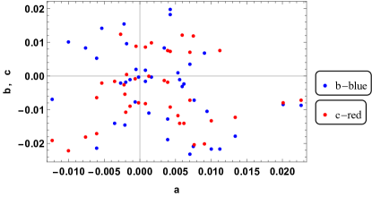
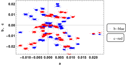
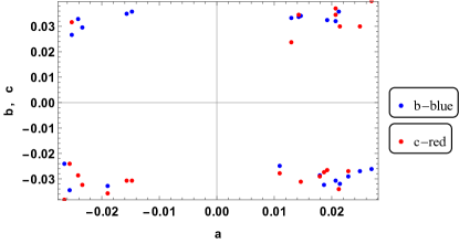
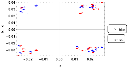
Figure 4: The graphical plots of allowed input elements a,b and c of a real Majorana mass texture generated by using Adaptive Monte Carlo simulation. Thin and thick plots (a),(b) and (c),(d) of the above figure represent scatter plots for rough solutions and enlarged solutions for the Majorana mass matrix in normal hierarchy(NH) and inverted hierarchy (IH) respectively.

When the set of six real numbers for imaginary part $\{a_{2},b_{2},c_{2},d_{2},e_{2},f_{2}\}$ is equal to zero, then complex symmetric matrix becomes a real symmetric matrix. For such real symmetric Majorana mass matrix, we also estimate all the elements in the mass matrix for both normal hierarchy (NH) and inverted hierarchy, and we then plot their frequency spectrum. The physical interpretation of frequency spectrum for the elements of the mass matrix is given for both normal hierarchy (NH) in Figure 1 and inverted hierarchy (IH) in Figure 2. In the case of NH, the frequency spectrum for the elements a, b, and c shows preferable small values nearer to centre from both sides on x-axis. The frequency spectrum for the elements d, e, and f shows preferable small non-zero values farther away from the centre of both sides on x-axis. The sine of three mixing angles found in both NH and IH shows two possible allowed frequency peaks on both sides of x-axis, which are shown in Figure 3. The observed pattern of the elements a, b, c, d, e, and f is found to be opposite in the case of IH. The graphical scatter plots for rough solutions of the elements a, b and c in NH and IH are shown in the Figures 4(a) and 4(c) respectively. The enlarged solutions for these elements are shown in Figure4(b)(NH) and Figure4(d)(IH). For such real symmetric Majorana mass matrix, we also study two zero texture classified as

$A_{1}:a,b=0$;

$A_{2}:a,c=0$;

$B_{1}:c,d=0$;

$B_{2}:b,f=0$;

$B_{3}:b,d=0$;

$B_{4}:c,f=0$ and

$C:d,f=0$.

These two zero texture are still allowed with the earlier cosmological Planck upper bound, $\sum|m_{i}|<0.23$ eV [31, 32] in both NH and IH mass models. The latest cosmological Planck upper bound, $\sum|m_{i}|<0.12$ eV allows in only the case of two zero texture for $A_{1}$ and $A_{2}$.

Parameter	I	II	III	IV
$\Delta m_{31}^{2}[eV^{2}]$	$2.44\times 10^{-3}$	$2.47\times 10^{-3}$	$2.43\times 10^{-3}$	$2.48\times 10^{-3}$
$\Delta m_{21}^{2}[eV^{2}]$	$7.29\times 10^{-5}$	$7.21\times 10^{-5}$	$7.56\times 10^{-5}$	$7.48\times 10^{-5}$
$|m_{1}|$	0.01669	0.01471	0.00713	0.01789
$|m_{2}|$	0.01875	0.01699	0.01124	0.01987
$|m_{3}|$	0.05214	0.05189	0.04985	0.053
$|U_{e1}|$	0.8407	0.8332	0.8357	0.8298
$|U_{e2}|$	0.5206	0.5325	0.5282	0.5385
$|U_{e3}|$	0.1488	0.1488	0.1502	0.1457
$|U_{\mu 1}|$	0.3421	0.3785	0.4053	0.3703
$|U_{\mu 2}|$	0.5852	0.5999	0.6121	0.5995
$|U_{\mu 3}|$	0.7351	0.7048	0.6789	0.7094
$|U_{\tau 1}|$	0.4197	0.4030	0.3705	0.4173
$|U_{\tau 2}|$	0.6216	0.5970	0.5883	0.5919
$|U_{\tau 3}|$	0.6613	0.6935	0.7186	0.6895
$\theta_{12}/^{0}$	31.76	32.58	32.29	32.98
$\theta_{13}/^{0}$	8.55	8.55	8.64	8.37
$\theta_{23}/^{0}$	48.02	45.46	43.37	45.81
$\delta_{CP}/^{0}$	256.21	263.74	265.86	257.41
$\alpha/^{0}$	175.75	101.64	94.46	83.56
$\beta/^{0}$	177.76	247.49	477.02	287.00
$\sum|m_{i}|[eV]$	0.08759	0.0836	0.06824	0.09077

Table 3: The best central values of the neutrino oscillation parameters within 3$\sigma$ bound of experimental data calculated by using Adaptive Monte Carlo method in NH. All the neutrino oscillation parameters are found within 3$\sigma$ bound of experimental data consistent with the latest Planck cosmological upper bound $\sum|m_{i}|<0.12$ eV.

Parameter	I	II	III	IV
$\Delta m_{32}^{2}[eV^{2}]$	$2.55\times 10^{-3}$	$2.53\times 10^{-3}$	$2.56\times 10^{-3}$	$2.53\times 10^{-3}$
$\Delta m_{21}^{2}[eV^{2}]$	$7.36\times 10^{-5}$	$7.19\times 10^{-5}$	$7.41\times 10^{-5}$	$7.98\times 10^{-5}$
$|m_{1}|$	0.05045	0.05056	0.05017	0.04976
$|m_{2}|$	0.05117	0.05127	0.05090	0.05055
$|m_{3}|$	0.00813	0.0098	0.00512	0.00483
$|U_{e1}|$	0.8330	0.8288	0.8324	0.8238
$|U_{e2}|$	0.5322	0.5406	0.5335	0.5450
$|U_{e3}|$	0.1508	0.1435	0.1499	0.1554
$|U_{\mu 1}|$	0.3620	0.3611	0.3584	0.3728
$|U_{\mu 2}|$	0.6329	0.6001	0.5802	0.6445
$|U_{\mu 3}|$	0.6843	0.7137	0.7313	0.6674
$|U_{\tau 1}|$	0.4183	0.4272	0.4226	0.4269
$|U_{\tau 2}|$	0.5621	0.5894	0.6154	0.5361
$|U_{\tau 3}|$	0.7134	0.6855	0.6653	0.7282
$\theta_{12}/^{0}$	32.57	33.11	32.65	33.48
$\theta_{13}/^{0}$	8.67	8.25	8.62	8.94
$\theta_{23}/^{0}$	43.8	46.15	47.7	42.5
$\delta_{CP}/^{0}$	246.14	251.96	259.74	241.41
$\alpha/^{0}$	149.51	48.09	119.88	89.27
$\beta/^{0}$	244.69	130.54	388.35	394.59
$\sum|m_{i}|[eV]$	0.1097	0.1116	0.1062	0.1051

Table 4: The best central values of the neutrino oscillation parameters within 3$\sigma$ bound of experimental data calculated by using Adaptive Monte Carlo method in IH. All the neutrino oscillation parameters are found within 3$\sigma$ bound of experimental data consistent with the latest Planck cosmological upper bound $\sum|m_{i}|<0.12$ eV.

Parameter	$a=0$	$a,b=0$	$a,c=0$
$\Delta m_{32}^{2}[eV^{2}]$	$2.46\times 10^{-3}$	$2.43\times 10^{-3}$	$2.53\times 10^{-3}$
$\Delta m_{21}^{2}[eV^{2}]$	$7.42\times 10^{-5}$	$7.59\times 10^{-5}$	$7.39\times 10^{-5}$
$|m_{1}|$	0.00285	0.00504	0.00522
$|m_{2}|$	0.00907	0.01	0.01
$|m_{3}|$	0.04968	0.04958	0.06587
$|U_{e1}|$	0.8411	0.8263	0.8214
$|U_{e2}|$	0.5209	0.5442	0.5517
$|U_{e3}|$	0.1451	0.1447	0.1441
$|U_{\mu 1}|$	0.3163	0.3761	0.4241
$|U_{\mu 2}|$	0.6235	0.6325	0.5406
$|U_{\mu 3}|$	0.7149	0.6769	0.7204
$|U_{\tau 1}|$	0.4386	0.4190	0.3811
$|U_{\tau 2}|$	0.5828	0.5518	0.6281
$|U_{\tau 3}|$	0.6839	0.7216	0.6783
$\theta_{12}/^{0}$	31.76	33.36	33.88
$\theta_{13}/^{0}$	8.34	8.32	8.28
$\theta_{23}/^{0}$	46.26	43.17	46.72
$\delta_{CP}/^{0}$	231.54	246.73	246.80
$\alpha/^{0}$	8.36	119.03	131.8
$\beta/^{0}$	360.40	499.94	420.12
$\sum|m_{i}|[eV]$	0.06162	0.06470	0.06587

Table 5: The best central values of the neutrino oscillation parameters for zero texture within 3$\sigma$ bound of experimental data calculated by using Adaptive Monte Carlo method. All the neutrino oscillation parameters are found within 3$\sigma$ bound of experimental data consistent with the latest Planck cosmological upper bound $\sum|m_{i}|<0.12$ eV.

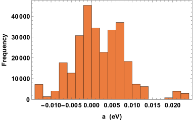
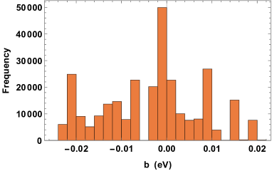
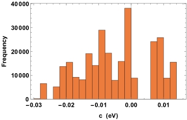
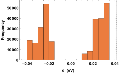
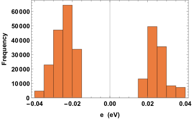
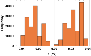
Figure 1: Frequency spectrum for the elements of the neutrino mass matrix in normal mass hierarchy (NH). The numerical values in region of higher peak of frequency spectrum shows more possible solutions as compared to lower peak region of the frequency spectrum.

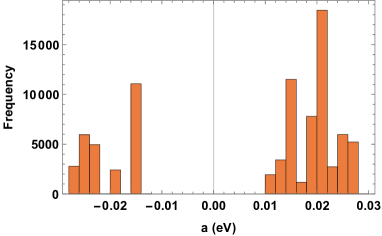
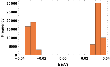
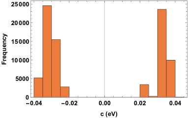
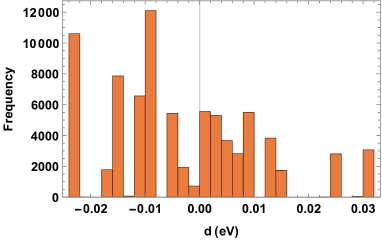
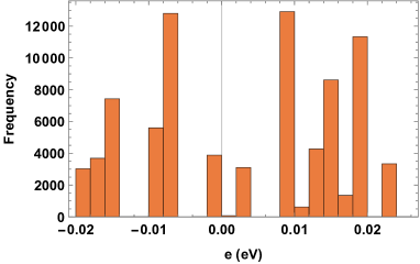
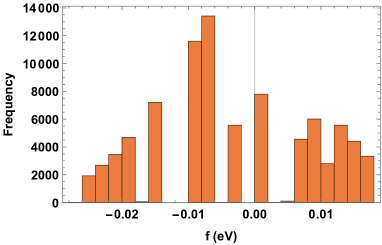
Figure 2: Frequency spectrum for the elements of the neutrino mass matrix in inverted mass hierarchy (IH). The numerical values in region of higher peak of frequency spectrum shows more possible solutions as compared to lower peak region of the frequency spectrum.

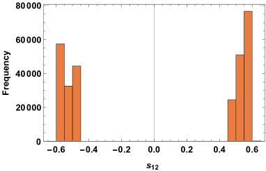
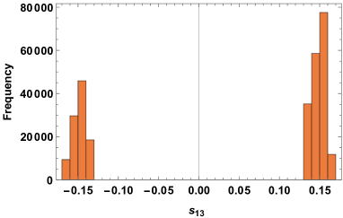
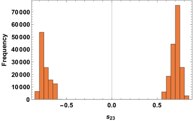
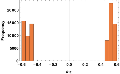
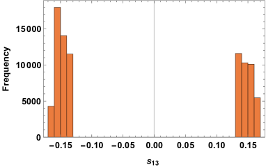
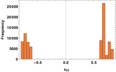
Figure 3: (a)-(c) represent frequency spectrum for sine of the three mixing angles in normal hierarchy (NH) and (d)-(f) represent frequency spectrum for sine of the three mixing angles in inverted hierarchy (NH). The numerical values in region of higher peak of frequency spectrum shows more possible solutions as compared to lower peak region of the frequency spectrum.

4 Summary and conclusion

To summarize, we use the Adaptive Monte Carlo method for numerical analysis where the elements of Majorana neutrino mass matrix are randomly generated. The Majorana neutrino mass matrix should be complex matrix in order to account for the CP violating Dirac phase. A complex symmetric mass matrix is essentially considered for CP non-conserving case. Twelve parameters are required to construct a complex symmetric Majorana mass matrix. These twelve parameters correspond to three mass eigenvalues ($m_{1},m_{2},m_{3}$), three mixing angles ($\theta_{12},\theta_{13},\theta_{23}$), three CP violating phases ($\delta_{CP},\alpha,\beta$) and three non-physical phases ($\phi_{1},\phi_{2},\phi_{3}$) which can be absorbed by the charged fermion Dirac fields.

In numerical analysis, twelve parameters are represented by real numbers in such a way that $a=a_{1}+ia_{2},b=b_{1}+ib_{2},c=c_{1}+ic_{2},d=d_{1}+id_{2},e=e_{1}+ie_{2},f=f_{1}+if_{2}$. The set of twelve real numbers is randomly generated to construct a general Majorana mass matrix structure. A Hermitian matrix is formed by using the complex symmetric mass matrix so that direct digonalization of the Hermitian matrix leads to the exact mixing matrix constructed by the eigenvectors of the Hermitian matrix and the corresponding mass-squared eigenvalues. The main result of the numerical analysis shows that both normal and inverted hierarchical mass models with all non-zero elements are still valid within 3$\sigma$ bound of experimental data, consistent with the latest Planck upper mass bound, $\sum|m_{i}|<0.12$ eV. Some studies[33, 34] have also indicated the most constraining bound to date, $\sum|m_{i}|<0.09$ eV. When we impose this bound in our numerical analysis, there is no solution for the neutrino mass matrix in IH. Our numerical analysis also confirms the mass bound for both pure normal hierarchical and pure inverted hierarchical mass model ( $\sum|m_{i}|\sim 0.06\text{eV};m_{1}=0$ and $\sum|m_{i}|\sim 0.1\text{eV};m_{3}=0$ ) calculated by using the two mass-squared differences of the experimental best fit values.

The present numerical analysis is also extended to study some zero texture. The one zero texture, a=0 is only allowed in NH mass model. Two zero texture are also studied in both normal and inverted hierarchical mass models. A $3\times 3$ Majorana mass structure can have fifteen two zero texture. Out of the fifteen possible zero texture, only two cases for $a,b=0$ and $a,c=0$ are allowed in normal hierarchical mass model. None of these two zero texture is allowed in inverted hierarchical mass model. The present finding may have important implications for model building using discrete flavour symmetries.

References

- [1] E Kh Akhmedov, GC Branco, and MN Rebelo. Seesaw mechanism and structure of neutrino mass matrix. Physics Letters B, 478(1-3):215–223, 2000.
- [2] Keith R Dienes, Emilian Dudas, and Tony Gherghetta. Light neutrinos without heavy mass scales: A higher-dimensional seesaw mechanism. Nuclear Physics B, 557(1-2):25–59, 1999.
- [3] André De Gouvêa. Neutrino mass models. Annual Review of Nuclear and Particle Science, 66:197–217, 2016.
- [4] Yi Cai, Juan Herrero García, Michael A Schmidt, Avelino Vicente, and Raymond R Volkas. From the trees to the forest: a review of radiative neutrino mass models. Frontiers in Physics, 5:63, 2017.
- [5] Stephen F King, Alexander Merle, Stefano Morisi, Yusuke Shimizu, and Morimitsu Tanimoto. Neutrino mass and mixing: from theory to experiment. New Journal of Physics, 16(4):045018, 2014.
- [6] M Concepción González-Garciá and Yosef Nir. Neutrino masses and mixing: evidence and implications. Reviews of Modern Physics, 75(2):345, 2003.
- [7] B Dziewit, K Kajda, J Gluza, and M Zrałek. Majorana neutrino textures from numerical considerations: The c p conserving case. Physical Review D, 74(3):033003, 2006.
- [8] Ken Kiers, Jeff Kolb, John Lee, Amarjit Soni, and Guo-Hong Wu. Ubiquitous cp violation in a top-inspired left-right model. Physical Review D, 66(9):095002, 2002.
- [9] Biswajit Adhikary, Mainak Chakraborty, and Ambar Ghosal. Masses, mixing angles and phases of general majorana neutrino mass matrix. Journal of High Energy Physics, 2013(10):1–25, 2013.
- [10] Shivani Gupta, Sin Kyu Kang, and CS Kim. Renormalization group evolution of neutrino parameters in presence of seesaw threshold effects and majorana phases. Nuclear Physics B, 893:89–106, 2015.
- [11] Cecilia Jarlskog. Commutator of the quark mass matrices in the standard electroweak model and a measure of maximal cp nonconservation. Physical Review Letters, 55(10):1039, 1985.
- [12] Maria Concepcion Gonzalez-Garcia, Michele Maltoni, and Thomas Schwetz. Nufit: three-flavour global analyses of neutrino oscillation experiments. Universe, 7(12):459, 2021.
- [13] Ivan Esteban, MC Gonzalez-Garcia, Michele Maltoni, Ivan Martinez-Soler, and Jordi Salvado. Updated constraints on non-standard interactions from global analysis of oscillation data. Journal of High Energy Physics, 2018(8):1–33, 2018.
- [14] Ivan Esteban, Maria Conceptión González-García, Michele Maltoni, Thomas Schwetz, and Albert Zhou. The fate of hints: updated global analysis of three-flavor neutrino oscillations. Journal of High Energy Physics, 2020(9):1–22, 2020.
- [15] Victoria Puyam, S Robertson Singh, and N Nimai Singh. Deviation from tribimaximal mixing using a4 flavour model with five extra scalars. Nuclear Physics B, 983:115932, 2022.
- [16] Stefano Morisi and José WF Valle. Neutrino masses and mixing: a flavour symmetry roadmap. Fortschritte der Physik, 61(4-5):466–492, 2013.
- [17] F Gonzalez Canales, A Mondragon, and M Mondragon. The s3 flavour symmetry: Neutrino masses and mixings. Fortschritte der Physik, 61(4-5):546–570, 2013.
- [18] Nabila Aghanim, Yashar Akrami, Mark Ashdown, J Aumont, C Baccigalupi, M Ballardini, AJ Banday, RB Barreiro, N Bartolo, S Basak, et al. Planck 2018 results-vi. cosmological parameters. Astronomy & Astrophysics, 641:A6, 2020.
- [19] Isabelle Tanseri, Steffen Hagstotz, Sunny Vagnozzi, Elena Giusarma, and Katherine Freese. Updated neutrino mass constraints from galaxy clustering and cmb lensing-galaxy cross-correlation measurements. Journal of High Energy Astrophysics, 36:1–26, 2022.
- [20] H Nishiura, K Matsuda, and T Fukuyama. Lepton and quark mass matrices. Physical Review D, 60(1):013006, 1999.
- [21] Walter Grimus, Anjan S Joshipura, Luıs Lavoura, and Morimitsu Tanimoto. Symmetry realization of texture zeros. The European Physical Journal C-Particles and Fields, 36:227–232, 2004.
- [22] Ivan Esteban, Maria Conceptión González-García, Alvaro Hernandez-Cabezudo, Michele Maltoni, and Thomas Schwetz. Global analysis of three-flavour neutrino oscillations: synergies and tensions in the determination of 23, cp, and the mass ordering. Journal of High Energy Physics, 2019(1):1–35, 2019.
- [23] Zhi-zhong Xing and Zhen-hua Zhao. The minimal seesaw and leptogenesis models. Reports on Progress in Physics, 84(6):066201, 2021.
- [24] M Agostini, M Allardt, Erica Andreotti, AM Bakalyarov, M Balata, I Barabanov, M Barnabé Heider, N Barros, L Baudis, C Bauer, et al. Results on neutrinoless double- decay of ge 76 from phase i of the gerda experiment. Physical Review Letters, 111(12):122503, 2013.
- [25] Matteo Agostini, GR Araujo, AM Bakalyarov, M Balata, I Barabanov, L Baudis, C Bauer, E Bellotti, S Belogurov, A Bettini, et al. Final results of gerda on the search for neutrinoless double- decay. Physical review letters, 125(25):252502, 2020.
- [26] M Agostini, AM Bakalyarov, M Balata, I Barabanov, L Baudis, C Bauer, E Bellotti, S Belogurov, Alice Bettini, L Bezrukov, et al. Improved limit on neutrinoless double- decay of ge 76 from gerda phase ii. Physical review letters, 120(13):132503, 2018.
- [27] K-H Ackermann, M Agostini, M Allardt, M Altmann, E Andreotti, AM Bakalyarov, M Balata, I Barabanov, M Barnabé Heider, N Barros, et al. The gerda experiment for the search of 0 decay in 76 ge. The European Physical Journal C, 73:1–29, 2013.
- [28] Max Aker, Konrad Altenmüller, M Arenz, M Babutzka, J Barrett, S Bauer, M Beck, A Beglarian, J Behrens, T Bergmann, et al. Improved upper limit on the neutrino mass from a direct kinematic method by katrin. Physical review letters, 123(22):221802, 2019.
- [29] Max Aker, Konrad Altenmüller, Marius Arenz, Woo-Jeong Baek, John Barrett, Armen Beglarian, Jan Behrens, Anatoly Berlev, Uwe Besserer, Klaus Blaum, et al. First operation of the katrin experiment with tritium. The European Physical Journal C, 80:1–18, 2020.
- [30] M Aker, K Altenmüller, JF Amsbaugh, M Arenz, M Babutzka, J Bast, S Bauer, H Bechtler, M Beck, A Beglarian, et al. The design, construction, and commissioning of the katrin experiment. Journal of Instrumentation, 16(08):T08015, 2021.
- [31] Planck Collaboration, PA Ade, N Aghanim, M Arnaud, M Ashdown, J Aumont, C Baccigalupi, AJ Banday, RB Barreiro, E Battaner, et al. Planck intermediate results xxiv. constraints on variations in fundamental constants? Astronomy & Astrophysics/Astronomie et Astrophysique, 580, 2015.
- [32] Peter AR Ade, Nabila Aghanim, M Arnaud, Mark Ashdown, J Aumont, Carlo Baccigalupi, AJ Banday, RB Barreiro, JG Bartlett, Nicola Bartolo, et al. Planck 2015 results-xiii. cosmological parameters. Astronomy & Astrophysics, 594:A13, 2016.
- [33] Eleonora Di Valentino, Stefano Gariazzo, and Olga Mena. Most constraining cosmological neutrino mass bounds. Physical Review D, 104(8):083504, 2021.
- [34] Eleonora Di Valentino and Alessandro Melchiorri. Neutrino mass bounds in the era of tension cosmology. The Astrophysical Journal Letters, 931(2):L18, 2022.