Revealed preference and revealed preference cycles:
a survey
Abstract
Afriat’s Theorem (1967) states that a dataset can be thought of as being generated by a consumer maximizing a continuous and increasing utility function if and only if it is free of revealed preference cycles containing a strict relation. The latter property is often known by its acronym, GARP (for generalized axiom of revealed preference). This paper surveys extensions and applications of Afriat’s seminal result. We focus on those results where the consistency of a dataset with the maximization of a utility function satisfying some property can be characterized by a suitably modified version of GARP.
Keywords: GARP, SARP, acyclicity, revealed preferences, utility maximization, rationalization, consumer choice
1 Introduction
Revealed preference analysis is built upon the observation that a utility maximizer who purchases a consumption bundle when bundle was cheaper is revealing that is preferred to (i.e. yields more utility than ). Thus, for instance, utility maximization prohibits a consumer from revealing that is preferred to (i.e. purchasing when was cheaper) and later on revealing that is preferred to (purchasing when is cheaper). This simple prohibition on cycles in the revealed preference relation is naturally extended to the generalized axiom of revealed preference (GARP) which states that there is no sequence of bundles where is revealed preferred to which is revealed preferred to and so on up to and further is revealed preferred to .
While it is obvious that utility maximizers satisfy GARP, Afriat’s Theorem (Afriat (1967)) establishes that GARP is more than just a consequence of utility maximization, it is rather the only consequence in the sense that whenever a consumer satisfies GARP there exists some well-behaved utility function which explains the consumer’s purchases. As we shall see, GARP-style acyclicity conditions play a fundamental role in the revealed preference literature and this fundamental role is the focus of the present survey.
Revealed Preferences and Acyclicity.
To elaborate further we introduce some notation. Suppose we observe a consumer purchase consumption bundle (a vector with an entry reporting the quantity consumed of each good) when prices are (a vector with an entry reporting the price of each good) for some . We write and say that is revealed preferred to if the bundle costs less than in observation . Similarly, we write and say that is strictly revealed preferred to if the bundle costs strictly less than in observation . GARP then is the requirement that the revealed preference relations and do not contain cycles in the sense that there is no sequence of observations so that
| (1) |
Afriat’s Theorem shows that GARP characterizes well-behaved utility maximization in the sense that there exists an increasing and continuous utility function which explains the behavior of the consumer (i.e. in each observation the bundle chosen yields more utility than any other affordable bundle) if and only if the consumer satisfies GARP.
Many of the assumptions involved in Afriat’s Theorem can be relaxed without substantially changing the result. For instance, Reny (2015) shows that even when the dataset has infinitely many observations (whether countable or uncountable) GARP is necessary and sufficient for a dataset to be rationalized by an increasing utility function. Similarly, Forges and Minelli (2009) show that a natural extension of GARP characterizes well-behaved utility maximization when the consumer is faced with non-linear prices. Polisson and Quah (2013) show that while a utility maximizer may violate GARP when the consumption space is discrete (i.e. all goods can only be consumed in non-negative integer quantities) this conclusion is reversed when there is at least one (potentially unobserved) divisible good for the consumer to purchase. Nishimura, Ok, and Quah (2017) show that the maximization of utility function that is increasing in a given ordering of interest (such as ordering by first order stochastic dominance over the space of simple lotteries) can be characterized by a suitable modified version of GARP.
A related acyclicity condition known as SARP characterizes well-behaved utility maximization with single-valued demand (instead of a demand correspondence). To define SARP let us write to mean that was cheaper than in observation and in addition . The consumer’s behavior satisfies the strong axiom of revealed preference (SARP) if is acyclic in the sense that there is no sequence so that . Matzkin and Richter (1991) and Lee and Wong (2005) show that SARP characterizes well-behaved utility maximization with demand functions in the sense that there exists a well-behaved utility function which generates a demand function (i.e. the set of consumption bundles which maximize the utility function on any given linear budget set is singleton) if and only if the consumer satisfies SARP.
It is easy to come up with purchases which satisfy SARP and nevertheless cannot be explained as the result of a consumer maximizing a differentiable utility function. Thus, if one wishes to explain purchasing behavior as the result of differentiable utility maximization, it is not enough that the consumer satisfies SARP. Chiappori and Rochet (1987) and Matzkin and Richter (1991) show that if consumer satisfies SARP and in addition implies for all observations then there exists an increasing and infinitely differentiable utility function which generates a demand function and which explains the purchasing behavior of the consumer.
The previously mentioned results are surveyed in Sections 2 and 3. Section 4 collects various results which do not fit cleanly into the previous sections. Included in this latter section is a discussion of (i) the issue of imperfect utility maximization as embodied by the cost-efficiency approach of Afriat (1973), (ii) a model of approximate utility maximization which turns out to be characterized by acyclicity of the strict revealed preference relation , (iii) a model in which expenditure directly enter the utility function, and (iv) the role of acyclicity conditions in mechanism design.
What we do not cover.
Our survey focuses on acyclicity conditions because these conditions play a fundamental role in the revealed preference literature and because this focus allows us to keep the paper relatively concise. The downside of this focus is that we inevitably neglect many important results in the revealed preference literature which do not involve acyclicity conditions. Here we briefly mention some of the important works which we do not cover in detail. This will at least provide the relevant references for the interested reader. We also refer the reader to the excellent book on revealed preference theory by Chambers and Echenique (2016).
Hurwicz and Uzawa (1971) provide necessary and sufficient conditions on a demand function (as opposed to a finite set of choices) in order for this demand function to be generated by a well-behaved utility function. Varian (1983) characterizes utility maximization where the utility function is required to be homothetic, weakly separable, or additively separable. Diewert and Parkan (1985) extend the weakly separable result in Varian (1983). Cherchye et al. (2015) show how Varian’s test for weak separability can be implemented as an integer programming problem.
Green and Srivastava (1986) and Kubler et al. (2014), building on Varian (1983), characterize expected utility maximization with concavity and Polisson et al. (2020) characterize expected utility maximization without concavity. Echenique and Saito (2015) characterize subjective (i.e. the state probabilities are not given) expected utility maximization. Echenique et al. (2019) characterize exponential discounted utility. For an excellent survey of the revealed preference literature for choice under risk, uncertainty, and time see Echenique (2020).
Browning (1989) characterizes additive across-period utility maximization (i.e. the utility function takes the form where is consumption in period ). Interestingly, it is shown in Brown and Calsamiglia (2007) that the same condition found in Browning (1989) also characterizes quasilinear utility maximization. Quasilinear utility maximization is further investigated in Castillo and Freer (2023) and Allen and Rehbeck (2021b).
There is also a related literature covering testing in economic equilibrium models which is surveyed in Carvajal (2024). Brown and Matzkin (1996) study testable restrictions in an exchange economy. This analysis is extended in Brown and Shannon (2000) who study the testable restriction of competitive equilibria, and Carvajal (2010) who extends the analysis to competitive economies with externalities. Cherchye et al. (2007) and Cherchye et al. (2010) characterize the behavioral consequences of the collective household model presented in Browning and Chiappori (1998). Carvajal et al. (2013) characterize the testable implications of Cournot competition.
2 Rationalizable behavior in a market setting
2.1 Afriat’s Theorem
We begin our discussion with Afriat’s Theorem. To set the stage, we assume that there are goods that can be purchased in any non-negative quantity and a consumer who purchases a bundle of the goods , where is the quantity of good consumed. A preference relation is a complete and transitive binary relation.111The binary relation is complete if or for all and is transitive if and implies for all . A utility function is any function that maps the consumption bundles into the real line . Each utility function generates a preference relation by defining so that if and only if for all . We next discuss the observables.
We observe a purchase dataset of the form where denotes the consumption bundle selected by the consumer in period under the prevailing prices where is the price of good in period . We wish to know if the consumer selected the consumption bundles in to maximize utility. More formally, we wish to know if can be rationalized by a utility function in the sense that, for all , the bundle chosen yields more utility than any other affordable bundle, i.e.
| (2) |
A more modest objective is to determine if there exists a preference relation which rationalizes the data in the sense that, for all , the bundle chosen is preferred to any other affordable bundle, i.e.
If rationalizes then the preference relation generated by also rationalizes and thus the concept of a utility rationalization is more demanding than that of a preference rationalization.
Without additional restrictions there are no testable implications of utility or preference maximization. In particular, every dataset can be rationalized by (i) the preference relation in which the consumer is indifferent between all consumption bundles and (ii) a constant utility function. Thus, we ought to entertain some additional properties of preference relations and utility functions.
Here are some properties we might like to impose on our rationalizing preference relations and utility functions. A preference relation is locally non-satiated if, for every bundle and every neighborhood of there exists some so that (where means and ). The function is increasing if implies and implies . The function is strictly increasing if implies .222As usual, for and we write to mean for all , we write to mean and , and we write to mean for all . A strictly increasing utility function obviously generates a locally non-satiated preference relation and thus a dataset which can be rationalized by a strictly increasing utility function can also be rationalized by a locally non-satiated preference relation.
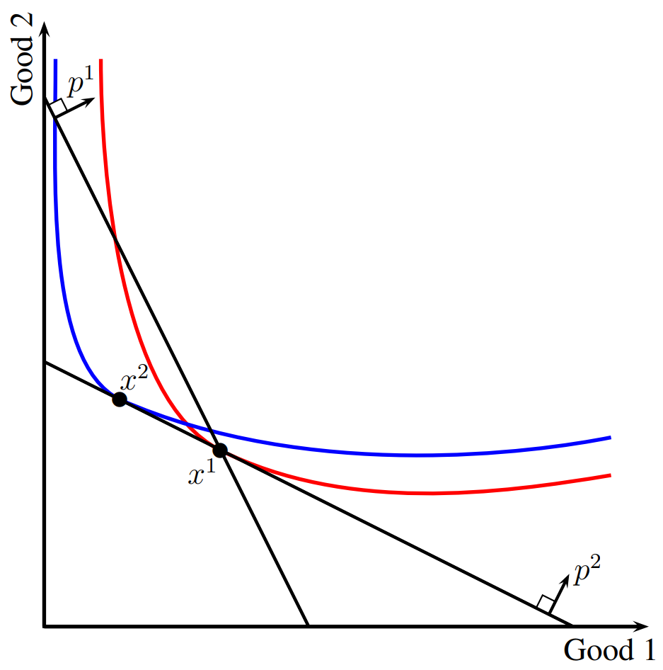
While every purchase dataset can be rationalized by a constant utility function it is easy to construct datasets which cannot be rationalized by strictly increasing utility functions. For example, let be the two observation dataset depicted in Figure 1. We see that is weakly cheaper than in period 2 (i.e. ) and is strictly cheaper than in period 2 (i.e. . Any strictly increasing utility function which rationalizes must, because of the second observation, satisfy and must, because of the first observation, satisfy . These two requirements are clearly incompatible. Another way of showing that this dataset cannot be rationalized by a strictly increasing utility function is to note that any strictly increasing utility function which rationalizes this dataset would have indifference curves tangent to the budget lines at the selected bundles. However, as shown in the figure, any such indifference curves would have to cross, which is not allowed by any increasing utility function.
From the previous discussion the following facts are immediate; (i) if a consumer buys bundle when is weakly cheaper then it must be that and (ii) if a consumer buys bundle when is strictly cheaper then it must be that . This serves as the motivation for the following revealed preference relations. We write and say that is revealed preferred to if is weakly cheaper than in period , i.e. and further we write and say that is strictly revealed preferred to if is strictly cheaper than in period , i.e. . From (i) and (ii) above we see that, every strictly increasing utility function which rationalizes must satisfy
| (3) |
From (3) it is clear that if can be rationalized by a strictly increasing utility function then the revealed preference relations must be acylic in the following sense.
Definition 1 (GARP).
The purchase dataset satisfies the generalized axiom of revealed preference (GARP) if there are no sequences so that
| (4) |
To see that utility maximizers with strictly increasing utility functions always satisfy GARP let us suppose that is rationalized by a strictly increasing utility function and suppose there is some sequence so that (4) holds (i.e. GARP is violated). From (3) we have and so we obtain the absurdity and the claim is proved. Surprisingly, GARP is also sufficient. The following is Afriat’s Theorem from Afriat (1967) (see also Diewert (1973) and Varian (1982)).333Recall that a function is concave if for all and .
Theorem 1 (Afriat, 1967).
For any purchase dataset , the following statements are equivalent.
-
1.
The dataset can be rationalized by a locally non-satiated preference relation.
-
2.
The dataset satisfies GARP.
-
3.
There are numbers and strictly positive numbers such that
(5) -
4.
The data can be rationalized by a continuous, concave, and strictly increasing utility function.
The implication 1 4 shows that any dataset which can be rationalized by a locally non-satiated preference relation can also be rationalized by a continuous, concave, and strictly increasing utility function. Thus, there are no testable implications of utility maximization by a continuous, concave, and strictly increasing utility function beyond what is already implied by the maximization of a locally non-satiated preference relation. Statement 3 establishes that GARP can be verified by solving a simple linear programming problem and thus determining if a given dataset satisfies GARP is computationally straightforward.
Proofs of Afriat’s Theorem may be found in Afriat (1967), Varian (1982), Fostel et al. (2004), and Polisson and Renou (2016). Below we provide our own self-contained proof which is inspired by the proof in Quah (2014). Showing 4 1 and 1 2 in Afriat’s Theorem is trivial. To show that 3 4 we assume that we have found some numbers and strictly positive numbers which satisfy (5) and then define by . It happens that this satisfies the properties required in Statement 4. Thus, the main difficulty in proving Afriat’s Theorem lies in showing 2 3. The approach we take is to define the numbers and strictly positive numbers recursively (in other words we define then we define as a function of and then we define as a function of and and then we define as a function of all the previously defined numbers, and so forth). As we shall see, an appropriately specified recursive formula is enough to produce the desired numbers.
Proof of Afriat’s Theorem..
As every strictly increasing utility function generates a locally non-satiated preference relation it is clear that 4 1. We next show 1 2. Suppose is rationalized by locally non-satiated preference relation . As rationalizes we see that implies . Further, if then there exists some neighborhood of so that for all . As is locally non-satiated there exists so that and thus, as rationalizes , we see that and so we have seen that implies and implies for all and . As is transitive it is now obvious that GARP holds and so we have shown that 1 2.
We next show 2 3. We write if there exists so that (so is the transitive closure of ). Let denote the strict part of (that is, means and ). Let be the number of elements in the longest sequence satisfying (so, is the number of elements in the longest path beginning at in the ordering). Reorder the observations if needed so that . We define recursively via
{IEEEeqnarray}rCl
u^i & = min( { u^j + λ^j p^j ⋅(x^k - x^j): ∀j,k s.t. —j— ¡ —i— and —k— = —i— } ∪{0} )
λ^i = max( { uj- uipi⋅(xj- xi) : ∀j s.t. —j— ¡ —i— } ∪{ 1 } )
Note that in (2.1) only depends on and for and thus only depends on . Similarly, in (2.1) only depends on and where and thus the numbers are indeed define recursively. Note that implies that and thus and so (2.1) never involves division by . From these remarks it is clear that the numbers are well-defined. Next, note that and thus satisfies the requirement of being strictly positive. We next confirm that the numbers satisfy (5).
Let . If then (5) follows immediately from (2.1) (take ). If then it is obvious that and because satisfies GARP we have (this is in fact the only time GARP is invoked) and so (5) holds. Finally, if then (using (2.1) with )
and so the numbers satisfy (5) and thus we have proved 2 3.
To complete the proof we need to show 3 4. Take any numbers , for , which satisfy (5) and define by
| (6) |
which is continuous, concave, and strictly increasing as it is the pointwise minimum of a finite number of continuous, concave, and strictly increasing functions. It remains to show that rationalizes . Take any and such that or, equivalently, . Then,
This concludes our proof of Theorem 1. ∎
We conclude this subsection with some remarks.
Remark 1.
Let us say that the dataset satisfies the weak axiom of revealed preferences (WARP) if there are no observations and so that and . While it is clear that a dataset which satisfies GARP also satisfies WARP surprisingly, as shown by Rose (1958) and Banerjee and Murphy (2006), when there are only two goods (so ) the reverse implication also holds. That is, when GARP and WARP are equivalent and so, under these conditions, we can confirm that the dataset can be rationalized by a strictly increasing, continuous, and concave utility function by checking that satisfies WARP.
Remark 2.
Kitamura and Stoye (2018), building on McFadden and Richter (1991) (see also McFadden (2005)), characterize random utility maximization when we observe the distribution of demand over a finite number of linear budget sets. That is, suppose there are sets where, for each , we have for some price vector and some expenditure level . For each , let denote a probability measure concentrated on . A random utility model (RUM) is a distribution over strictly increasing utility functions. The RUM rationalizes if, for each and for all Borel sets the probability is equal to the probability with which a utility function drawn from has an optimum over which is inside . Kitamura and Stoye (2018) provide necessary and sufficient conditions for to be rationalized by a RUM.
Remark 3.
Richter (1966) characterizes preference maximization using a stronger notion of what it means for a preference to rationalize behavior. Let be some collection of non-empty subsets of and let be a correspondence with domain which satisfies for each . Intuitively, represents the choices which the consumer finds acceptable when confronted with constraint set . Let us say that the preference relation strictly rationalizes if, for all , we have . In other words, in order for to strictly rationalize we require that the set of bundles chosen are exactly the best bundles in according .
Let us write if there exists such that and (in other words, was chosen when was available). Also, write if there exists such that , , and (in other words, was chosen and was not chosen). The choice correspondence satisfies the congruence axiom if, there is no sequence such that
It is easy to see that the congruence axiom is necessary for to be strictly rationalized by a preference relation. Richter (1966) shows that the congruence axiom is also sufficient. In fact, Richter’s result holds for any consumption space (not just the space of consumption bundles ) and, in this respect, the result is similar to the result of Nishimura et al. (2017) which we present below as Theorem 6.
2.2 SARP and demand functions
The utility function supplied by Afriat’s Theorem does not in general generate a single-valued demand function. To be specific, let be the demand generated by utility function with the constraint of spending no more than when prices are , i.e.
| (7) |
where is the budget set . Even when is a continuous, concave, and strictly increasing utility function (these being the properties possessed by the utility function supplied by Statement 4 in Afriat’s Theorem), the demand may be non-singleton for some values of . Here we investigate how to test for utility maximization which generates demand functions (in other words, is a singleton for all ).
We can also define the demand generated by a preference relation. Specifically, the preference relation generates the demand defined by
| (8) |
We shall also be interested in conditions under which the data can be rationalized by a preference relation which generates a demand function.
If the purchase data is rationalized by a utility function which generates a demand function then clearly, for each , the utility derived from strictly exceeds the utility derived from any other affordable bundle. This suggests introducing the revealed preference relation where means that is some affordable bundle distinct from (i.e. and ). Clearly,
| (9) |
where is any utility function which rationalizes the data and which generates a demand function. Notice that the relation is almost equivalent to the defined in the previous subsection, but applies only to bundles different from , i.e., we have , but not . From (9) it is clear that if can be rationalized by a utility function which generates a demand function then the relation must be acyclic in the following sense.
Definition 2 (SARP).
The purchase dataset satisfies the strong axiom of revealed preferences (SARP) if, there is no sequence so that
| (10) |
While SARP is obviously a necessary condition in order for the data to be rationalized by a utility function which generates a demand function it happens that SARP is also sufficient. A version of the following theorem was originally stated in Matzkin and Richter (1991) and later improved upon in Lee and Wong (2005).444Recall that a function is strictly concave if for all and .
Theorem 2 (Matzkin and Richter, 1991 and Lee and Wong, 2005).
For any purchase dataset , the following statements are equivalent.
-
1.
can be rationalized by a preference relation which generates a demand function.
-
2.
satisfies SARP.
-
3.
There are numbers satisfying implies for all and strictly positive numbers such that
(11) -
4.
can be rationalized by a continuous, strictly concave, and strictly increasing utility function which generates an infinitely differentiable demand function.
Here we provide a sketch of the proof of Theorem 2. Implications 4 1 and 1 2 are obvious. To show 2 3 we re-purpose the proof from Section 2.1. Indeed, let be defined as in this proof and define numbers and by
{IEEEeqnarray}rCl
u^i & = min( { u^j + λ^j p^j ⋅(x^k - x^j) - 1: ∀j,k s.t. —j— ¡ —i— and —k— = —i— } ∪{0} )
λ^i = max( { uj- ui+ 1 pi⋅(xj- xi) : ∀j s.t. —j— ¡ —i— } ∪{ 1 } )
The numbers and can be shown to be well-defined using the arguments we used to show that the numbers defined in (2.1) and (2.1) are well-defined. Also, note that for all and so to finish our proof of 2 3 we must verify that and satisfy (11).
Let . If then (11) follows immediately from (2) (take ). If then it is obvious that and, if further then, because satisfies SARP, it must be that and therefore and so (11) holds. Finally, if then (using (2) with )
and so the numbers satisfy (11) and thus we have proved 2 3.
To show 3 4 we follow the arguments in Matzkin and Richter (1991). The utility can be constructed as follows. First, take any function that is strictly convex and differentiable with , for all , and satisfies if, and only if, .555 For, example , for some . There is a sufficiently small number such that the function
is continuous, strictly concave, strictly increasing, and rationalizes the data. Since is continuous and strictly concave this utility function generates a demand function. This demand function will not in general be infinitely differentiable and so we fall short of delivering the utility function promised in statement 4. For the complete proof of 3 4 we refer the reader to Lee and Wong (2005) where a more complex construction is used to produce the desired utility function.
2.3 Rationalizability with a differentiable utility
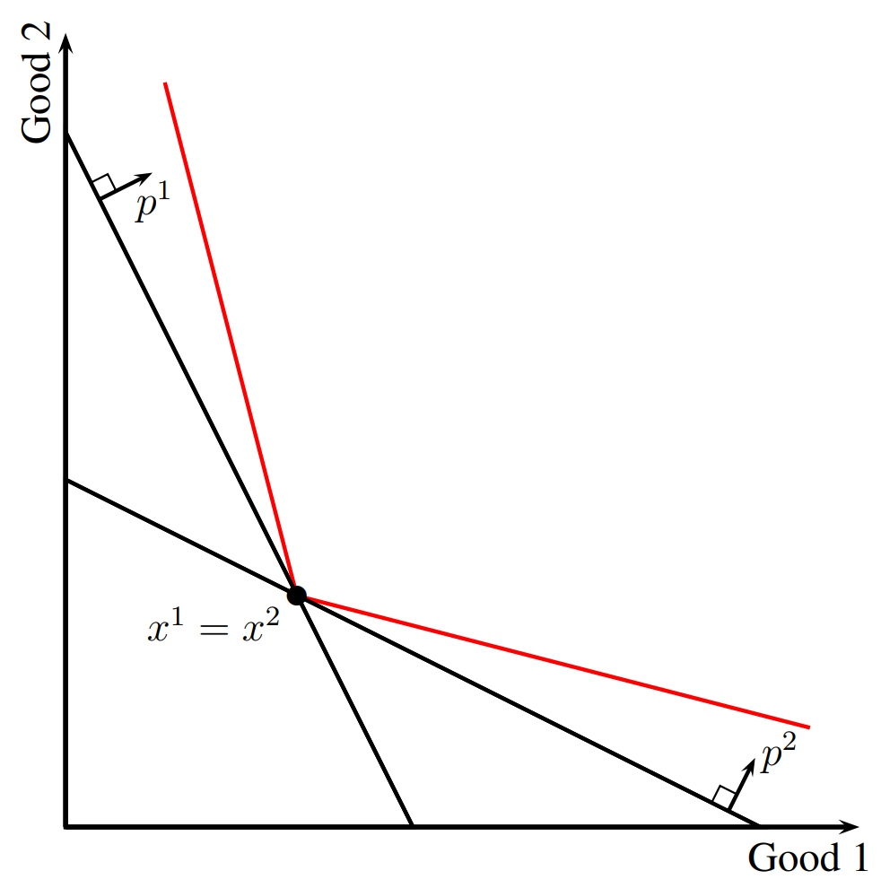
Neither GARP nor SARP are sufficient for a dataset to be rationalized by a differentiable utility function. Consider the example depicted in Figure 2. Since the consumer selected the same bundle under different prices, the data satisfies both GARP and SARP. However, any utility function rationalizing such a dataset would have an indifference curve with a kink at . Thus, it would not be differentiable at this particular point. As shown in Chiappori and Rochet (1987) and Matzkin and Richter (1991), it is possible to strengthen SARP into a sufficient condition for a differentiable rationalization.
Theorem 3 (Chiappori and Rochet, 1987 and Matzkin and Richter, 1991).
Suppose that the purchase dataset satisfies SARP and implies , for all . Then, can be rationalized by a strictly increasing, strictly concave, and infinitely differentiable utility function .666The domain of is the non-open set and so we should be clear about what it means for to be infinitely differentiable. We say that is infinitely differentiable if there exists some infinitely differentiable with domain (instead of ) so that is the restriction of to .
The rationalizing utility function supplied in Chiappori and Rochet (1987) is strictly increasing, strictly concave, and infinitely differentiable but its domain is some compact set satisfying . Matzkin and Richter (1991) in their Theorem extend the result of Chiappori and Rochet (1987) to what we state in our Theorem 3.
Theorem 3 provides a sufficient but not necessary condition for a dataset to be rationalized by a differentiable utility function (with some additional properties). In fact, from Theorem in Matzkin and Richter (1991) it is clear that if the dataset contains no purchases on the boundary of the consumption space (i.e. for all ) then the condition in Theorem 3 is necessary and sufficient. In other words, if it happens that for all then can be rationalized by a strictly increasing, strictly concave, and infinitely differentiable utility function if and only if (i) the data satisfies SARP and (ii) the data satisfies implies , for all .
See also Ugarte (2023) who finds a necessary and sufficient condition under which a dataset can be rationalized by a differentiable, concave (but not necessarily strictly concave), and strictly increasing utility function.
2.4 Discrete Consumption
From Afriat’s Theorem we know that GARP is a necessary and sufficient condition for a dataset to be rationalized by a utility function with domain . This no longer holds when the consumption space is some subset of . For example, suppose that and let the dataset consist of observations , , , and . Note that in period 1 good 1 is more expensive and yet the consumer buys only this expensive good whereas in period 2 good 2 is more expensive and yet again the consumer only buys the expensive good. This clearly violates GARP (indeed, and ) and yet the data can be rationalized by the strictly increasing utility function .777To see that rationalizes the data note first that and next note that the affordable bundles in period 1 are , , and and so both and give the largest utility among the affordable bundles and similarly the affordable bundles in period 2 are , , and and so again and give the largest utility among the affordable bundles.
This example highlights an important distinction between utility maximization and cost minimization. As and in the example it is clear that any rationalizing utility function must assign bundles and the same level of utility. However, this means that in each observation, the consumer is spending more money than necessary, by purchasing the more expensive bundle. Polisson and Quah (2013) propose an alternative model of consumer choice that induces choices consistent with GARP.
Proposition 1 (Polisson and Quah, 2013).
Let and let be a purchase dataset with for all . Suppose there is a function , a strictly increasing function , positive numbers , and strictly positive numbers and such that, for all , we have
Then, the purchase dataset satisfies GARP.
The message of Proposition 1 is that as long as the consumer maximizes some overall utility that includes a divisible good, the observations of the prices and the demands of the goods in obey GARP, even when the space is discrete.
The intuition behind Proposition 1 is fairly straightforward. Because there is a divisible good (and is strictly increasing) the consumer cannot be cost-inefficient (i.e. in each period they must reach the attained utility level in the cheapest way possible) as any misspent money could be reallocated to the divisible good resulting in an increase in utility. From this observation it is clear that (3) holds and so GARP must also hold.
It is worth pointing out that Proposition 1 imposes no assumptions on the function . In particular, it need not be increasing or concave. Moreover, given that obeys GARP, one can apply Afriat’s Theorem to show that it can be rationalized by a strictly increasing utility function. In fact, as highlighted in the result below, GARP allows us to rationalize the dataset with a utility function that is quasilinear with respect to the (unobserved) divisible good.
Proposition 2 (Polisson and Quah, 2013).
Let and suppose that the dataset satisfies GARP. Then, there exists a function such that:
-
1.
rationalizes the dataset ;
-
2.
is consistent with the relations and in the sense of (3);
-
3.
admits a concave and strictly increasing extension to ;
-
4.
There are strictly positive numbers and such that, for all ,
The proof of this result follows almost immediately from Afriat’s Theorem. GARP guarantees that is rationalizable by a strictly increasing and concave function defined as in (6) over the entire positive orthant . Moreover, the function is consistent with the directly revealed preference relations and . Clearly, this implies that once we restrict to , it satisfies conditions 1–3.
To show that condition 4 holds take any , for all , and define , where is the number used in the definition of in (6). Notice that, for any , , and that satisfy , we obtain
and so condition 4 holds.
2.5 Rationalizing infinite datasets
Up to this point we have only considered datasets consisting of finitely many observations . Here we relax this restriction and allow for purchase datasets , where is an arbitrary index set and thus may contain infinitely many elements. As before, a utility function rationalizes the purchase dataset if (2) holds. The revealed preference relations and are defined as in Section 2 and the definition of GARP is the same as before. Reny (2015) shows that GARP remains necessary and sufficient for an increasing rationalization even when there are infinitely many observations.888Recall that a function is quasiconcave if for all .
Theorem 4 (Reny, 2015).
Let be an arbitrary (possible infinite) purchase dataset. The following statements are equivalent.
-
1.
can be rationalized by a locally non-satiated preference relation .
-
2.
satisfies GARP.
-
3.
can be rationalized by an increasing and quasiconcave utility function .
Note that, although GARP remains necessary and sufficient for a dataset to be rationalized with an increasing utility function, Theorem 4, in contrast to the utility function supplied in Afriat’s Theorem, no longer guarantees that the function is continuous, strictly increasing, and concave.
Reny (2015) shows through counterexamples that there is little room for strengthening the properties imposed on the rationalizing utility function without imposing further conditions on the data (beyond GARP). In particular, Reny constructs GARP-satisfying datasets so that cannot be rationalized by an increasing and lower semicontinuous utility function; cannot be rationalized by an increasing and upper semicontinuous utility function; and cannot be rationalized by an increasing and concave utility function.999To our knowledge, it is an open question as to whether Reny’s result could be strengthened to allow for a quasiconcave and strictly increasing rationalization. Put another way, Afriat’s Theorem demonstrates that the hypothesis that utility is continuous, concave, and strictly increasing imposes no additional testable implications on finite purchase datasets beyond what is imposed by the hypothesis that preferences are locally non-satiated. This conclusion is reversed for infinite observation datasets where these properties yield additional testable implications.
Below, we present a slightly modified version of Example 2 from Reny (2015) which shows that there is a GARP-satisfying purchase dataset which cannot be rationalized by an increasing and upper semicontinuous utility function.101010Recall that a function is upper semicontinuous if, for all convergent sequences , we have .
Example 2.
There are two goods, i.e., . The purchase dataset consists of elements , , and , , for . It is easily verified that , for all and so the data satisfies GARP. For a contradiction suppose that is rationalized by an increasing and upper-semicontinuous utility function . As rationalizes it must satisfy (3) and because for all we see that . Since , upper semicontinuity requires that . However, as , it must be that and so we conclude which is a contradiction. Therefore, cannot be rationalized by an increasing and upper-semicontinuous utility function.
3 Rationalization in general frameworks
3.1 Non-linear prices
Up to this point prices have been linear. For instance, if one buys the bundle it costs twice as much as the bundle . Here we consider how to characterize utility maximizing behavior when prices are not necessarily linear. A price function is a continuous and strictly increasing function where, intuitively, represents the price of (the expenditure associated with) the bundle . We consider a purchase dataset of the form where is the consumption bundle purchased by the consumer when faced with the price function .
As before, a utility function rationalizes if, for each , the utility derived from exceeds the utility of any other affordable bundle, i.e., for all satisfying . Similarly, a preference relation rationalizes if, for all , the bundle chosen is preferred to every other affordable bundle (i.e. for all satisfying ). Note that if all price functions are positive linear functions (i.e. for some price vector ) then our dataset is as in Section 2 and thus Afriat’s Theorem applies. In fact, even when are not linear a version of GARP still characterizes strictly increasing utility maximization.
We define and in essentially the same way as in Section 2. To be precise, means was affordable when was purchased (i.e. ) and means was cheaper than in period (i.e. ). It is easy to see that (3) holds for all strictly increasing and rationalizing utility functions and thus if can be rationalized by a strictly increasing utility function then satisfies GARP (where GARP continues to be as in Definition 1 only now using our generalized definitions of and ). As shown in Forges and Minelli (2009) the reverse implication also holds.111111The functions in Forges and Minelli (2009) are normalized so that . This normalization has no impact on the result in Theorem 5 and can easily be imposed if so desired by defining by and working with the normalized dataset .,121212The functions do not have to represent prices. Instead, can be thought of as any function which describes the constraint set faced by the consumer in period in the sense that in each period the consumer must select a bundle in the constraint set . Forges and Minelli (2009) provide some analysis of the types of constraint sets which can be described in this fashion.
Theorem 5 (Forges and Minelli, 2009).
For any dataset the following statements are equivalent.
-
1.
The dataset can be rationalized by a locally non-satiated preference relation.
-
2.
The dataset satisfies GARP.
-
3.
There are numbers and strictly positive numbers such that
-
4.
The dataset can be rationalized by a continuous and strictly increasing utility function.
Implication 4 is obvious. Implication 1 2 and implication 2 3 can be shown using a similar approach to what we employed in our proof of Afriat’s Theorem (just replace and with and , respectively in equations (2.1) and (2.1)). Finally, given the numbers , it is easy to prove that the function
| (12) |
is strictly increasing, continuous, and rationalizes the data.
The utility function supplied in statement 4 of Theorem 5 is not concave whereas the utility function in statement 4 of Afriat’s Theorem is concave. Indeed, when prices are non-linear concave and strictly increasing utility has additional testable restrictions beyond GARP. However, if the price functions are concave then the utility function constructed in (12) is also concave and thus GARP is necessary and sufficient for a concave, strictly increasing, and continuous rationalization when each of the price functions also satisfy these properties. A version of this observation was presented originally in Matzkin (1991) in a setup with differentiable rationalizations (as in Section 2.2). See also Cherchye et al. (2014) for a study of the testable implications of concave rationalizations.
Theorem 5 is largely unchanged even when the dataset has infinitely many observations. In particular, suppose we have a dataset where is an arbitrary index set and are prices functions. In this context Reny (2015) shows that GARP is necessary and sufficient for there to exist an increasing utility function which rationalizes the data.
3.2 Generalized Monotonicity and Abstract Choice Spaces
Consider an arbitrary consumption space and suppose the researcher observes a choice dataset , where is an arbitrary index set and denotes an alternative selected from the constraint set (and so, we require for all ). The choice dataset is rationalized by utility function if, for any , the bundle chosen yields more utility than any other bundle which could have been chosen (i.e. for all ). Alternatively, the dataset is rationalized by the preference relation if the bundle selected is preferred to every other bundle which could have been chosen (i.e. for all ). When and each constraint set takes the form for some price vector then our new notion of rationalization coincides with the old one.
As in the preceding sections, unless we impose some additional restrictions, any dataset is rationalizable with a constant utility . For this reason we restrict our attention to utilities that are strictly increasing with respect to some ordering on . For example, within Euclidean spaces it may be sensible to consider preferences in which “more is better”, i.e., we have . When studying choice under risk, the natural order is that of first order stochastic dominance over lotteries. When studying choice over time, one could consider the order of impatience (specified below in Example 4). Here we present general results that are applicable to a great variety of such orderings.
Formally, let be a preorder on , i.e., a reflexive and transitive binary relation, with its asymmetric part denoted by .131313So, means and . A utility function is strictly -increasing if implies , and implies . Similarly, a preference relation over is strictly -increasing if implies , and implies .141414Note that the concept of “strictly -increasing” (where is the usual Euclidean order on ) is the same as what we simply refer to as “strictly increasing.” Below we present two examples of relevant economic setups.
Example 3.
Suppose there are states of the world and let represent a state contingent consumption bundle where denotes the amount of consumption (or money) received in state . Let be a probability vector (i.e. ) which represents the likelihood of the different states of the world occurring. A state-contingent consumption bundle first order stochastically dominates if, for each number the probability that pays out more than is greater than the probability that pays out more than . Let us write it as , with its strict part denoted by . It is natural (and required by many models of consumer choice under risk) to think that a consumer should prefer to whenever . In other words, the utility function of a consumer ought to be -strictly increasing.
Example 4.
Suppose there are two time periods and let denote a stream of consumption where is the amount of consumption (or money) received now and is the amount of consumption received later. It is natural to think that an impatient consumer should prefer the stream to , whenever . This preference for receiving larger amounts earlier can be summarized with a preorder. Specifically, let denote the smallest preorder which extends the natural partial order over , and satisfies , for all .151515We say that a binary relation extends a second binary relation if implies . The existence of the preorder is easy to establish. Let be the preorder defined by , for any . It is easy to see that is the transitive closure of .
As in the preceding sections, it is convenient to discuss the testable restrictions of utility maximization by first introducing some revealed preference relations. Let be an arbitrary space endowed with a preorder and let be a (possibly infinite) choice dataset. We write if there exists such that , in other words, when is chosen over an alternative that dominates with respect to the ordering . Note that if then , but our definition of allows for not to belong to . Similarly, we write if there exists such that , in other words, when is chosen over an alternative that strictly dominates with respect to .161616Notice that, within the original setup of Afriat (1967) (as in Section 2.1) or Forges and Minelli (2009) (as in Section 3.1), the revealed preference relations coincide exactly with , defined in the corresponding sections.
It is straightforward to show that (3) holds (replacing and with and ) provided is strictly -increasing and rationalizes the data. Indeed, suppose that . By definition of the relation, there is so that . Since rationalizes and is -strictly increasing, we have and so as claimed. A similar argument establishes that implies . From these observations we see that the following acyclicity condition holds whenever the data can be rationalized by a strictly -increasing utility function.
Definition 3 (-GARP).
A dataset satisfies the generalized axiom of revealed preferences for (henceforth, -GARP) if there is no sequence in such that
| (13) |
Note that, as in the original formulation of GARP, the above condition excludes particular cycles induced by the revealed preference relations. In fact, within the setup of Afriat (1967) (as in Section 2.1) or Forges and Minelli (2009) (as in Section 3.1), -GARP coincide exactly with GARP, whenever we set .
It is clear that -GARP is necessary for a dataset to be rationalizable with a -strictly increasing preference relation. As shown in Nishimura et al. (2017) it happens to also be sufficient.
Theorem 6.
Let be an arbitrary space endowed with a preorder and let be a choice dataset. The data can be rationalized by a strictly -increasing preference relation if, and only if, it satisfies -GARP.
Necessity of -GARP for rationalization follows from our previous discussion. The proof of sufficiency involves applying Szpilrajn’s extension theorem to the transitive closure of . While Theorem 6 shows that -GARP is enough to find a strictly -increasing preference relation which rationalizes the data, the theorem does not claim that this preference relation can be represented by a utility function. In order to guarantee this, more structure must be imposed on the data and the choice space. The following is from Nishimura et al. (2017).
Theorem 7.
Let be a separable and locally compact metric space and let be a continuous preorder.171717 This is to say that is a closed subset of . Moreover, suppose that the dataset has finitely many observations (i.e. the index set is finite) and the set is compact, for all . Then, the dataset can be rationalized by a continuous and strictly -increasing utility function if and only if satisfies -GARP.
Importantly, is a separable and locally compact metric space and thus Theorem 7 can be used to recover part of Afriat’s Theorem. Note however that the consumption space in this theorem is not a vector space and so, unlike Afriat’s Theorem, it has nothing to say about the concavity of the rationalizing utility function.
The proof that -GARP is sufficient for a dataset to be rationalized by a continuous and -strictly increasing utility can be carried out by applying Levin’s Theorem. This theorem states that any continuous preorder admits a complete extension that can be represented with a continuous utility function. The proof of Theorem 7 proceeds by first showing that the transitive closure of is a continuous preorder and then completing this preorder by applying Levin’s Theorem. The final step involves checking that this preorder (equivalently, the continuous utility function that is its representation) rationalizes the data.
The theorem’s feature of allowing the rationalizing utility function to be increasing in an order of interest has proven to be useful in applied studies. Polisson et al. (2020) use Theorem 7 to test for utility maximization over lotteries where the utility function is required to be increasing in the ordering of first order stochastic dominance and Lanier et al. (2022) use Theorem 7 to test for utility maximization over risky temporal streams of consumption where various orders of interest are imposed on the rationalizing utility function.
Example 3 (continued).
Suppose there are two equally likely states of the world, i.e., , and suppose we observe a consumer purchase the state-contingent consumption bundle under prices . Therefore, consist of a single observation . In particular, the set trivially satisfies GARP and, thus, Theorem 1 guarantees that there is a continuous, concave, and strictly increasing utility function which rationalizes the dataset.
However, one can easily check, that any such utility would not be consistent with the first order stochastic dominance order. Indeed, note that the bundle was affordable when was purchased under the prevailing prices. Therefore, any utility rationalizing the choice must satisfy . Given that , any such utility must violate first order stochastic dominance order. Therefore, the original formulation of GARP is not sufficient for this stricter form of rationalization. In contrast, -GARP provides the exact characterization of this model and this property is violated in this example, since .
4 Related results and extensions
In the previous sections we have shown that the essence of utility maximization and its testable implications are summarized with an acyclicity condition — the generalized axiom of revealed preference and its variations. In this section we consider several models that are, in one way or another, somewhat removed from the standard setup and show that GARP-like properties continue to play a role in their characterization.
4.1 Measuring departures from rationality
It is very common in empirical studies for purchase datasets to violate GARP and, thus, are not (exactly) consistent with utility maximization.181818See Chapter 5 in Chambers and Echenique (2016) for a general discussion on the empirical analysis. More recently, inconsistencies with utility maximization have been reported in Halevy et al. (2018), Echenique et al. (2019), Feldman and Rehbeck (2022), Zrill (2020), Dembo et al. (2021), and Cappelen et al. (2023). Perhaps this is not entirely surprising, given the deterministic nature of GARP, which is either satisfied by a dataset or not. When faced with a violation of GARP, one may be interested in measuring the severity of the dataset’s inconsistency with utility-maximization. Part of the revealed preference literature has been devoted to formulating and answering this question, which is obviously important for empirical applications.191919 See Afriat (1973), Houtman and Maks (1985), Varian (1990), Echenique et al. (2011), Dean and Martin (2016), Apesteguia and Ballester (2015), Echenique et al. (2018, 2020), Dziewulski (2020), Allen and Rehbeck (2020, 2021a), de Clippel and Rozen (2021), or Ribeiro (2023).
Arguably, the most common measure of departures from rationality is the critical cost-efficiency index (CCEI, also known as Afriat’s efficiency index), introduced in Afriat (1973) to evaluate violations of utility maximization within the standard consumer demand framework.202020Among others, CCEI was employed in Sippel (1997), Harbaugh et al. (2001), Andreoni and Miller (2002), Choi et al. (2007), Fisman et al. (2007), Ahn et al. (2014), Choi et al. (2014), Cherchye et al. (2017), Echenique et al. (2019), Cherchye et al. (2020), Dembo et al. (2021), and Cappelen et al. (2023). Consider the setup discussed in Section 2, where a purchase dataset is given by , with denoting a consumption bundle selected by the consumer under the prevailing prices . Take any number – an efficiency parameter – and define the following binary relation: , whenever , i.e., the bundle dominates in this sense if the former was chosen when the value of the latter was at most of the value of , under the prevailing prices. Analogously, we denote , whenever . Clearly, whenever , the above relations coincide with those defined in Section 2.1.
Given the relations , one can easily define an acyclicity condition analogous to GARP. The dataset satisfies GARP for the efficiency parameter (-GARP), if there is no sequence such that , and ; in other words, the relations and are required to obey the property highlighted in Definition 1. Clearly, -GARP is weaker than GARP in the sense that, the latter holds only if so does the former and, more generally, a dataset satisfies -GARP if it obeys -GARP for any . This is clear because and .
Clearly, -GARP is not sufficient for a dataset to be rationalizable with utility maximization. However, it characterizes a weaker notion of rationality.
Proposition 3.
Take any efficiency index . A dataset satisfies -GARP if, and only if, if there is a strictly increasing utility that -rationalizes , by which we mean the following: for all ,
Proofs of this proposition appear in Afriat (1973), Halevy et al. (2018), Polisson et al. (2020), and Lanier et al. (2022). This result says that -GARP is necessary and sufficient for the data to be partially rationalized in the sense that the observed choice gives higher utility than any bundle that costs less than of its value. This rationalization is only partial since it leaves open the possibility that, at some observation , a bundle valued between and gives higher utility than .212121This imperfect utility-maximization could also be interpreted as imperfect cost-minimization subject to a utility target (see Polisson and Quah (2022)). The CCEI is defined as the supremum over all efficiency indices for which the dataset admits -rationalization by a strictly increasing utility function.
Dziewulski (2020) shows that -rationalizations can be understood in terms of just-noticeable differences, in a model where consumers have limited ability to distinguish similar alternatives. In Cherchye et al. (2023), the CCEI is used in a statistical test of the utility maximization hypothesis. The notion of CCEI can be modified to measure the severity of a dataset’s departure from rationalization by utility functions satisfying specific properties. For example, we may be interested in the greatest at which can be -rationalized by a utility function that is strictly increasing with respect to some given preorder (as in Section 3.2); for applications of such an extension of the CCEI and a guide to its computation, see Polisson et al. (2020) and Lanier et al. (2022).
4.2 Acyclic strict preference relation
In some instances, one may consider the ‘weak’ revealed preference relation to be less informative of the agent’s true preferences than the strict preference . This may be due to a level of imprecision when stating indifferences or the subject’s inability to perfectly discriminate among similar alternatives. As a result, one may want to investigate implications of an acyclicity condition that is imposed solely on the strict revealed relation .
This is addressed in Dziewulski (2023). Formally, the condition requires that there is no sequence such that . The restriction implicitly assumes that only the revealed strict comparisons convey reliable information about the preferences of the individual, while the weak ones may be subject to imprecision, vagueness of judgement, or incommensurability. Therefore, only is required to exhibit some form of consistency. Dziewulski (2023) shows that acyclicity of is equivalent to the dataset being rationalizable with approximate utility maximization. That is, there is a utility and a positive threshold function such that (i) implies and (ii) implies , for all . The alternative is chosen only if its utility is at most utils lower than that of any other affordable option . This representation appeals to the idea of imperfect discrimination, suggesting that the individual discerns between two alternatives only if they yield a sufficiently different utility.222222 The reader may recognize that this model is following the interval order representation of preferences proposed in Fishburn (1970).
4.3 Revealed price preference
So far we have been focusing on how individuals reveal their preferences over consumption bundles. Deb et al. (2022) explore the implications of an agent who has a well-behaved revealed preference over prices. Suppose that we observe a consumer choosing bundle at prices , and at prices . The price is revealed preferred to , denoted by , whenever ; in other words, is revealed prefered to whenever the cost of purchasing bundle is lower at than at (the prevailing price at observation ). The revealed preference relation is said to be strict, and denoted by , whenever the cost is strictly lower.
Given the revealed preference relations , , one may be interested in exploring the implications of imposing a consistent condition on these relations. In particular, suppose , are free of cylces, in the sense defined in Section 2.1, i.e., there is no sequence such that and . Deb et al. (2022) show that this condition, dubbed the generalized axiom of price preference (or GAPP), is necessary and sufficient for the dataset to be rationalized with an expenditure-augmented utility function; formally, there is a strictly increasing utility such that , for all and . Notice that in this notion of rationalization, the consumer does not have a budget constraint and could (in principle) spend as much as he likes, but he does not spend an infinite amount because higher expenditure leads to dis-utility since the utility function has expenditure as its final argument and is strictly decreasing in expenditure. The expenditure-augmented utility function could be thought of as generalization of the familiar quasilinear form , for some increasing function .
4.4 GARP in mechanism design
Applications of the revealed preference theorems surveyed in this paper go beyond consumer/decision theory. Deb and Mishra (2014) apply this approach to study mechanism design.
Suppose an agent faces a mechanism designer232323Deb and Mishra (2014) consider multiple agents each with their own type-space and collection of utility functions. We consider a single agent because this significantly simplifies the presentation. who is unaware of the agent’s type . An agent of type has utility function where is some set of alternatives. A social choice function (SCF) maps types to alternatives. The output of the SCF is the alternative which the designer would like to select if she knew that the agent was type . To improve readability we write instead of .
A key assumption in Deb and Mishra (2014) is that, while the agent’s type is not observable, the payoff received by the agent from the alternative selected is observable and thus can be contracted on. A contingent contract is a collection where is strictly increasing for each . When the agent reports the contingent contract gives the agent with type a value of . In other words, the contingent contract rewards the agent according to (i) the report of the agent and (ii) the payoff that the agent actually derives from .242424It is true that a mechanism designer may surmise from the observed payoff that the agent has not reported his type truthfully; the assumption is that the contract must still reward the agent in a way that is strictly increasing in the agent’s payoff. For a discussion of this issue see Deb and Mishra (2014). The contingent contract is a linear contract if there are numbers and where and for all and .
We collect the utility functions and the social choice function into a dataset . We say that is implemented by the contingent contract if, for all the utility derived by the agent from reporting his true type is weakly larger than the utility he derives from any other report. That is, is implemented by if for all . Note that if the contingent contract is linear then this condition becomes
| (14) |
which has a similar structure to the Afriat inequalities of (5).
It turns out that can be implemented if and only if it satisfies a GARP-like acyclicity condition. We write to mean and further we write to mean . We say that is acyclic if the relations and satisfy the conditions in Definition 1 (i.e. there is no sequence so that , and ). The following is a version of Theorem 1 in Deb and Mishra (2014).252525Again we remark that Deb and Mishra (2014) allow for multiple agents and so their theorem is significantly more involved.
Theorem 8.
(for finite ) can implemented by a contingent contract if and only if it is acyclic. Moreover, if can be implemented by a contingent contract then it can be implemented by a linear contract.
5 Conclusion
Acyclicity conditions are often easily derived as necessary behavioral consequences of various models of utility maximization. It turns out that these simple conditions are remarkably powerful: as shown in this survey, very often they completely characterize the models of interest. This is true, not just of the classical model of consumer utility-maximization, but also of various extensions and variations of that model.
References
- Afriat (1967) Afriat, S. The construction of utility functions from expenditure data. International Economic Review, 8(1):67–77, 1967.
- Afriat (1973) Afriat, S. N. On a system of inequalities in demand analysis: An extension of the classical method. International Economic Review, 14(2):460–472, 1973.
- Ahn et al. (2014) Ahn, D., Choi, S., Gale, D., and Kariv, S. Estimating ambiguity aversion in a portfolio choice experiment. Quantitative Economics, 5(2):195–223, 2014.
- Allen and Rehbeck (2020) Allen, R. and Rehbeck, J. Satisficing, aggregation, and quasilinear utility. Working paper, 2020. Available at SSRN: https://ssrn.com/abstract=3180302.
- Allen and Rehbeck (2021a) Allen, R. and Rehbeck, J. Measuring rationality: Percentages vs expenditures. Theory and Decision, (forthcoming), 2021a.
- Allen and Rehbeck (2021b) Allen, R. and Rehbeck, J. Satisficing, aggregation, and quasilinear utility. 2021b.
- Andreoni and Miller (2002) Andreoni, J. and Miller, J. Giving according to GARP: An experimental test of the consistency of preferences for altruism. Econometrica, 70(2):737–753, 2002.
- Apesteguia and Ballester (2015) Apesteguia, J. and Ballester, M. A. A measure of rationality and welfare. Journal of Political Economy, 123(6):1278–1310, 2015.
- Banerjee and Murphy (2006) Banerjee, S. and Murphy, J. A simplified test for preference rationality of two-commodity choice. Experimental Economics, 9(1):67–75, 2006.
- Brown and Calsamiglia (2007) Brown, D. J. and Calsamiglia, C. The nonparametric approach to applied welfare analysis. Economic Theory, 31(1):183–188, 2007.
- Brown and Matzkin (1996) Brown, D. J. and Matzkin, R. L. Testable restrictions on the equilibrium manifold. Econometrica, 64(6):1249–1262, 1996.
- Brown and Shannon (2000) Brown, D. J. and Shannon, C. Uniqueness, stability, and comparative statics in rationalizable walrasian markets. Econometrica, 68(6):1529–1539, 2000.
- Browning (1989) Browning, M. A nonparametric test of the life-cycle rational expections hypothesis. International Economic Review, 30(4):979–992, 1989.
- Browning and Chiappori (1998) Browning, M. and Chiappori, P.-A. Efficient intra-household allocations: A general characterization and empirical tests. Econometrica, 66(6):1241–1278, 1998.
- Cappelen et al. (2023) Cappelen, A. W., Kariv, S., Sørensen, E. O., and Tungodden, B. The development gap in economic rationality of future elites. Games and Economic Behavior, 142:866–878, 2023.
- Carvajal (2010) Carvajal, A. The testable implications of competitive equilibrium in economies with externalities. Economic Theory, 45(1/2):349–378, 2010.
- Carvajal (2024) Carvajal, A. Recent advances on testability in economic equilibrium models. Journal of Mathematical Economics, 2024.
- Carvajal et al. (2013) Carvajal, A., Deb, R., Fenske, J., and Quah, J. K.-H. Revealed preference tests of the Cournot model. Econometrica, 81(6):2351–2379, 2013.
- Castillo and Freer (2023) Castillo, M. and Freer, M. A general revealed preference test for quasilinear preferences: theory and experiments. Experimental Economics, 26:673–696, 2023.
- Chambers and Echenique (2016) Chambers, C. P. and Echenique, F. Revealed preference theory. Econometric Society Monograph. Cambridge University Press, 2016.
- Cherchye et al. (2007) Cherchye, L., De Rock, B., and Vermeulen, F. The collective model of household consumption: A nonparametric characterization. Econometrica, 75(2):553–574, 2007.
- Cherchye et al. (2010) Cherchye, L., De Rock, B., and Vermeulen, F. An Afriat Theorem for the collective model of household consumption. Journal of Economic Theory, 145(3):1142–1163, 2010.
- Cherchye et al. (2014) Cherchye, L., Demuynck, T., and De Rock, B. Revealed preference analysis for convex rationalizations on nonlinear budget sets. Journal of Economic Theory, 152:224–236, 2014.
- Cherchye et al. (2015) Cherchye, L., Demuynck, T., De Rock, B., and Hjertstrand, P. Revealed preference tests for weak separability: An integer programming approach. Journal of Econometrics, 186(1):129–141, 2015.
- Cherchye et al. (2017) Cherchye, L., Demuynck, T., De Rock, B., and Vermeulen, F. Household consumption when the marriage is stable. American Economic Review, 107(6):1507–1534, 2017.
- Cherchye et al. (2020) Cherchye, L., De Rock, B., Surana, K., and Vermeulen, F. Marital matching, economies of scale, and intrahousehold allocations. Review of Economics and Statistics, 102(4):823–837, 2020.
- Cherchye et al. (2023) Cherchye, L., Demuynck, T., De Rock, B., and Lanier, J. Are Consumers (Approximately) Rational? Shifting the Burden of Proof. The Review of Economics and Statistics, (forthcoming), 2023.
- Chiappori and Rochet (1987) Chiappori, P.-A. and Rochet, J.-C. Revealed preferences and differentiable demand. Econometrica, 55(3):687–691, 1987.
- Choi et al. (2007) Choi, S., Fisman, R., Gale, D., and Kariv, S. Consistency and heterogeneity of individual behavior under uncertainty. American Economic Review, 97(5):1921–1938, 2007.
- Choi et al. (2014) Choi, S., Kariv, S., Müller, W., and Silverman, D. Who is (more) rational? American Economic Review, 104(6):1518–1550, 2014.
- de Clippel and Rozen (2021) de Clippel, G. and Rozen, K. Relaxed optimization: How close is a consumer to satisfying first-order conditions? Review of Economics and Statistics, 2021. (forthcoming).
- Dean and Martin (2016) Dean, M. and Martin, D. Measuring rationality with the minimum cost of revealed preference violations. Review of Economics and Statistics, 98(3):524–534, 2016.
- Deb and Mishra (2014) Deb, R. and Mishra, D. Implementation with contingent contracts. Econometrica, 82(6):2371–2393, 2014.
- Deb et al. (2022) Deb, R., Kitamura, Y., Quah, J. K. H., and Stoye, J. Revealed Price Preference: Theory and Empirical Analysis. The Review of Economic Studies, 90(2):707–743, 2022.
- Dembo et al. (2021) Dembo, A., Kariv, S., Polisson, M., and Quah, J. K.-H. Ever since Allais. Bristol Economics Discussion Papers 21/745, 2021. URL https://ideas.repec.org/p/bri/uobdis/21-745.html.
- Diewert (1973) Diewert, W. E. Afriat and revealed preference theory. The Review of Economic Studies, 40(3):419–425, 1973.
- Diewert and Parkan (1985) Diewert, W. and Parkan, C. Tests for the consistency of consumer data. Journal of Econometrics, 30(1):127–147, 1985.
- Dziewulski (2020) Dziewulski, P. Just-noticeable difference as a behavioural foundation of the critical cost-efficiency index. Journal of Economic Theory, 188(C), 2020.
- Dziewulski (2023) Dziewulski, P. A comprehensive revealed preference approach to approximate utility maximisation. Working paper, 2023.
- Echenique (2020) Echenique, F. New developments in revealed preference theory: Decisions under risk, uncertainty, and intertemporal choice. Annual Review of Economics, 12(1):299–316, 2020.
- Echenique and Saito (2015) Echenique, F. and Saito, K. Savage in the market. Econometrica, 83(4):1467–1495, 2015.
- Echenique et al. (2011) Echenique, F., Lee, S., and Shum, M. The money pump as a measure of revealed preference violations. Journal of Political Economy, 119(6):1201–1223, 2011.
- Echenique et al. (2018) Echenique, F., Imai, T., and Saito, K. Approximate expected utility rationalization. CESifo Working Paper Series 7348, 2018.
- Echenique et al. (2019) Echenique, F., Imai, T., and Saito, K. Decision making under uncertainty: An experimental study in market settings. Technical report, 2019. arXiv: 1911.00946.
- Echenique et al. (2020) Echenique, F., Imai, T., and Saito, K. Testable implications of models of intertemporal choice: Exponential discounting and its generalizations. American Economic Journal: Microeconomics, 12(4):114–143, 2020.
- Feldman and Rehbeck (2022) Feldman, P. and Rehbeck, J. Revealing a preference for mixtures: An experimental study of risk. Quantitative Economics, 13(2):761–786, 2022.
- Fishburn (1970) Fishburn, P. C. Intransitive indifference with unequal indifference intervals. Journal of Mathematical Psychology, 7:144–149, 1970.
- Fisman et al. (2007) Fisman, R., Kariv, S., and Markovits, D. Individual preferences for giving. American Economic Review, 97(5):1858–1876, 2007.
- Forges and Minelli (2009) Forges, F. and Minelli, E. Afriat’s theorem for general budget sets. Journal of Economic Theory, 144:135–145, 2009.
- Fostel et al. (2004) Fostel, A., Scarf, H., and Todd, M. Two new proofs of Afriat’s theorem. Economic Theory, 24(1):211–219, 2004.
- Green and Srivastava (1986) Green, R. and Srivastava, S. Expected utility maximization and demand behavior. Journal of Economic Theory, 38(2):313–323, 1986.
- Halevy et al. (2018) Halevy, Y., Persitz, D., and Zrill, L. Parametric recoverability of preferences. Journal of Political Economy, 126(4):1558–1593, 2018.
- Harbaugh et al. (2001) Harbaugh, W. T., Krause, K., and Berry, T. R. GARP for kids: On the development of rational choice behavior. American Economic Review, 91(5):1539–1545, 2001.
- (54) Hoderlein, S. and Stoye, J. Testing stochastic rationality and predicting stochastic demand: the case of two goods. Economic Theory Bulletin, 3:313–328.
- Hoderlein and Stoye (2014) Hoderlein, S. and Stoye, J. Revealed preferences in a heterogeneous population. The Review of Economics and Statistics, 96(2):197–213, 2014.
- Houtman and Maks (1985) Houtman, M. and Maks, J. A. H. Determining all maximal data subsets consistent with revealed preference. Kwantitative Methoden, 19:89–104, 1985.
- Hurwicz and Uzawa (1971) Hurwicz, L. and Uzawa, H. On the integrability of demand functions. In Chipman, J. S., Richter, M. K., and Sonnenschein, H. F., editors, Preferences, utility, and demand: A Minnesota symposium, chapter 6, pages 114–148. 1971.
- Kawaguchi (2017) Kawaguchi, K. Testing rationality without restricting heterogeneity. Journal of Econometrics, 197(1):153–171, 2017.
- Kitamura and Stoye (2018) Kitamura, Y. and Stoye, J. Nonparametric analysis of random utility models. Econometrica, 86(6):1883–1909, 2018.
- Kubler et al. (2014) Kubler, F., Selden, L., and Wei, X. Asset demand based tests of expected utility maximization. American Economic Review, 104(11):3459–80, 2014.
- Lanier et al. (2022) Lanier, J., Miao, B., Quah, J. K.-H., and Zhong, S. Intertemporal Consumption with Risk: A Revealed Preference Analysis. The Review of Economics and Statistics, (forthcoming), 2022.
- Lee and Wong (2005) Lee, P. M. H. and Wong, K.-C. Revealed preference and differentiable demand. Economic Theory, 25(4):855–870, 2005.
- Matzkin (1991) Matzkin, R. L. Axioms of revealed preference for nonlinear choice sets. Econometrica, 59(6):1779–1786, 1991.
- Matzkin and Richter (1991) Matzkin, R. L. and Richter, M. K. Testing strictly concave rationality. Journal of Economic Theory, 53(2):287–303, 1991.
- McFadden and Richter (1991) McFadden, D. and Richter, K. Stochastic rationality and revealed stochastic preference. In J. Chipman, D. M. and Richter, K., editors, Preferences, Uncertainty and Rationality. Westview Press, 1991.
- McFadden (2005) McFadden, D. L. Revealed stochastic preference: A synthesis. Economic Theory, 26(2):245–264, 2005.
- Nishimura et al. (2017) Nishimura, H., Ok, E. A., and Quah, J. K.-H. A comprehensive approach to revealed preference theory. American Economic Review, 107(4):1239–1263, 2017.
- Polisson and Quah (2013) Polisson, M. and Quah, J. K.-H. Revealed preference in a discrete consumption space. American Economic Journal: Microeconomics, 5(1):28–34, 2013.
- Polisson and Quah (2022) Polisson, M. and Quah, J. K. Rationalizability, cost-rationalizability, and Afriat’s efficiency index. Bristol Economics Discussion Papers 22/754, School of Economics, University of Bristol, UK, 2022. URL https://ideas.repec.org/p/bri/uobdis/22-754.html.
- Polisson and Renou (2016) Polisson, M. and Renou, L. Afriat’s theorem and Samuelson’s ‘eternal darkness’. Journal of Mathematical Economics, 65:36–40, 2016.
- Polisson et al. (2020) Polisson, M., Quah, J. K.-H., and Renou, L. Revealed preferences over risk and uncertainty. American Economic Review, 110(6):1782–1820, 2020.
- Quah (2014) Quah, J. A test for weakly separable preferences. Economics Series Working Papers 708, University of Oxford, Department of Economics, 2014.
- Reny (2015) Reny, P. J. A characterization of rationalizable consumer behavior. Econometrica, 83(1):175–192, 2015.
- Ribeiro (2023) Ribeiro, M. Comparative rationality. Working paper, 2023.
- Richter (1966) Richter, M. K. Revealed preference theory. Econometrica, 34(3):635–645, 1966.
- Rose (1958) Rose, H. Consistency of preference: The two-commodity case. Review of Economic Studies, 25(2):124–125, 1958.
- Sippel (1997) Sippel, R. An experiment of the pure theory of consumer behaviour. Economic Journal, 107(444):1431–1444, 1997.
- Ugarte (2023) Ugarte, C. Smooth rationalization. Working Paper, 2023.
- Varian (1982) Varian, H. R. The non-parametric approach to demand analysis. Econometrica, 50(4):945–973, 1982.
- Varian (1983) Varian, H. R. Non-parametric tests of consumer behaviour. The Review of Economic Studies, 50(1):99–110, 1983.
- Varian (1990) Varian, H. R. Goodness-of-fit in optimizing models. Journal of Econometrics, 46(1–2):125–140, 1990.
- Zrill (2020) Zrill, L. (non-)parametric recoverability of preferences and choice prediction. Working paper, 2020.