Integrating Multi-Physics Simulations and Machine Learning to Define the Spatter Mechanism and Process Window in Laser Powder Bed Fusion

Abstract

Laser powder bed fusion (LPBF) has shown promise for wide range of applications due to its ability to fabricate freeform geometries and generate a controlled microstructure. However, components generated by LPBF still possess sub-optimal mechanical properties due to the defects that are created during laser-material interactions. In this work, we investigate mechanism of spatter formation, using a high-fidelity modelling tool that was built to simulate the multi-physics phenomena in LPBF. The modelling tool have the capability to capture the 3D resolution of the meltpool and the spatter behavior. To understand spatter behavior and formation, we reveal its properties at ejection and evaluate its variation from the meltpool, the source where it is formed. The dataset of the spatter and the meltpool collected consist of 50 % spatter and 50 % melt pool samples, with features that include position components, velocity components, velocity magnitude, temperature, density and pressure. The relationship between the spatter and the meltpool were evaluated via correlation analysis and machine learning (ML) algorithms for classification tasks. Upon screening different ML algorithms on the dataset, a high accuracy was observed for all the ML models, with ExtraTrees having the highest at 96 % and KNN having the lowest at 94 %. Furthermore, the ML model was tested on a different dataset generated using FLOW-3D, a commercial, less computationally expensive tool, but lacks the capability to simulate realistic spatter formation. Our ML model trained on OpenFOAM dataset was able to classify the region of the meltpool in the FLOW-3D datasets as spatter initiation location. Upon screening 283 FLOW-3D simulation experiments with varying power-velocity combinations, a process map based on spatter volume was established. The process map will serve as a guide towards understanding how the process parameters influence part properties, identifying an AM process window with minimal defects and ultimately enhance repeatability in part production.

[inst1]organization=Department of Mechanical Engineering, Carnegie Mellon University,city=Pittsburgh, postcode=15213, state=PA, country=USA

[inst2]organization=Exentis Group AG,city=Stetten, postcode=5608, country=Switzerland

[inst3]organization=Department of Chemical Engineering, Carnegie Mellon University,city=Pittsburgh, postcode=15213, state=PA, country=USA [inst4]organization=Machine Learning Department, Carnegie Mellon University,city=Pittsburgh, postcode=15213, state=PA, country=USA

1 Introduction

Additive manufacturing (AM), commonly known as 3D printing, is a transformative approach to industrial production. Laser powder bed fusion (LPBF) is the most common metal AM process. It has several advantages in comparison to conventional manufacturing technologies like milling and casting. LPBF offers design flexibility, quick fabrication of prototypes directly from digital models, create less material waste and demonstrate onsite manufacturing capability. The process of using LPBF to create a 3D object starts with spreading a layer of metal particles on the build plate. Then the laser source moving at a certain power and velocity are guided by the laser scanners according to the information in the 3D CAD to melt the regions relating to the design, which then solidifies to form a single layer. The powder spreading, melting and solidifying processes will occur repeatedly until the final object is formed. LPBF has attracted applications in key economic sectors such as in medicine, automotive, aerospace, construction, energy and prototyping [1, 2]. However, when compared to other form of manufacturing such as machining, casting and rolling, AM currently has the lowest market share, which is as a result of poor repeatability, defect formations, and low productivity [1, 3]. Issues with poor repeatability can be attributed to various process parameters such as scanning speed, laser power, beam radius, gas flow, layer thickness, and hatch spacing involved in operating LPBF. Slight errors in these parameters can propagate, resulting in variability in part properties. Additionally, the multi-physics phenomena such as heat transfer, solidification, melting, vaporization and cooling that occur in AM further makes it a sensitive process [4, 5, 6].

Defects in LPBF could result from the process parameters that create the meltpool, and the common types are pore [7, 8, 9, 10, 11, 3, 12] and crack [13, 14, 15]. Pore defect can be divided into gas, lack-of-fusion (LOF) and keyhole-induced pore, and are differentiated by their natures and formation mechanism [16]. Spatter can lead to defects, especially to lack of fusion [13, 14, 15, 17]. Desire to implement multi-lasers to increase the productivity has been inhibited by spatter generation; an offshoot from the meltpool [18]. Their formation involves complicated interactions among high-speed vapor, vapor-induced powder motions and melt pool dynamics. Spatter can be the source of roughness and porosity on a part, and its detrimental effect could be reduced by manipulating the inert gas flow within the machine. However, reducing the quantity of spatter travelling during LPBF process requires optimum inert gas flow rate. High flow rate could lead to spatter generation from the powder bed, such that powder could be lifted by the inert gas, travel around the process chamber and land on a random location based on its trajectory, causing non-uniformity in the arrangement of the powder bed. It is challenging to establish optimum inert gas flow rate for spatter removal, also considering that the relationship will have to be established for varieties of power/velocity combinations which is not only time consuming but also expensive [5, 19, 14, 20]. Providing solution to spatter issues will require a holistic understanding of the physics of laser-material interactions, from melt pool creation to how the material properties can influence the intrinsic nature of the meltpool, leading to the instabilities that cause defect generation.

The two general approaches for investigating different phenomena in AM are advanced observational technologies and numerical simulation methods. Few experimental studies have been conducted on spatter, Barrett et al. [21] used high speed sterovision camera to capture spatter, then used computer vision to collect their properties for statistical analysis. Previous work by Chen et al. [13] revealed five categories of spatter that can be formed during LPBF: solid, metallic jet, powder agglomeration, entrainment melting spatter, and induced spatter. Additionally, they found that the size, speed and direction of the spatters vary based on the process condition. Nakamura et al. [22] also recorded the molten pool using in-situ X-ray monitoring with the support of tungsten carbide as tracers in high power laser welding of titanium alloy. They stressed that the upward melt flow around the keyhole surface drove liquid column formation, which could cause spatter generation. Qu et al. [23] report the elimination of large spatters through controlling laser-powder bed interaction instabilities by using nanoparticles. The elimination of large spatters results in 3D printing of defect lean samples with good consistency and enhanced properties. Although advanced monitoring methods have been used to investigate the formation mechanism of spatters through observation of the physical process, the quantitative relationship between spatter formation and the physical process is still difficult to establish due to the experimental limitations of resolution and dimensions. A trial-and-error experimental procedure for determining appropriate processing parameters is extremely time-consuming and costly, and it remains challenging to completely monitor the complex physical phenomena occurring in LPBF at microsecond and micrometer scales.

Numerical simulation can provide insights into regions where measurements are either difficult to collect or impossible. Additionally, it can offer three-dimensional, transient views of keyhole and molten pool behaviors that cannot be directly observed experimentally. Deng et al. [24] established a model of remote laser spiral spot welding to study the spatter formation. They found that the keyhole opening area serving as a main out-gassing channel and instantaneous vapor pressure impacting on the interface which are highly relevant with the spatter formation. Currently, many commercial simulation packages are available for AM, such as Ansys, Comsol multiphysics, and StarCCM+. However, these software lacks all the desired physical phenomenal that occur during AM. The available AM specific commercial software like FLOW-3D still require adjustments of various user numerical parameters, which sometimes are not accessible to the end-users. An open-source software like OpenFOAM (Open Field Operation and Manipulation) which is based on C++, is flexible in implementing additional features to address novel problems and processes occurring during AM process [25, 26].

In recent years, machine learning (ML) have gained increasing attention in AM due to its unprecedented performance in sub-category tasks, such as supervised, un-supervised and reinforcement learning [2, 27, 28, 29, 30]. In addition, the high computational cost associated with high-fidelity simulations has motivated their synergy with ML tools, especially where a large scale of simulation experiments is necessary, such as in understanding defect formation processes, part design optimization, and the discovery of metamaterials and process monitoring. [31, 32, 33, 34, 35, 36, 37, 38]. Hemmasian et al. [39] used FLOW-3D simulation software to create datasets for LPBF processes and trained them using a convolutional neural network to predict the three-dimensional temperature field solely by taking the process parameters and the time step as input. DebRoy et al. [40] combined physics-informed machine learning, mechanistic modeling, and experimental data to identify several important variables that reveal the physics behind the defect formation in AM, by considering an example of balling defects in LPBF using peer-reviewed experimental data available in the literature. It is therefore possible to extend AM modelling and simulation to a large scale and to cover a wide range of parameters. Ren et al. [11] used x-rays to track the formation of pores in LPBF while also making observations with a thermal imaging system. This setup allowed the authors to develop a high-accuracy method for detecting pore formation from thermal signature with the help of a machine learning method.

The potential for the synergy of ML with physics-based simulation to understand spatter formation remains unexploited, which could have been due to limited studies and understanding of spatter as compared to other form of defects. Spatter generation is influenced by complex and often nonlinear interactions between multiple process variables. ML models are adept at capturing these complex relationships in high-dimensional data. ML can provide predictive insights that are not easily discernible through traditional physics-based modeling. It can predict when and under what conditions spatter is likely to occur. Lastly, ML can help in optimizing the process parameters not just to avoid spatter but also to achieve the best possible outcomes in terms of speed, cost, and material properties. By employing ML models, a deeper understanding of spatter can be achieved leading to enhanced control, improved process efficiency, and superior material characteristics in manufacturing and other material processing fields. In this study, we develop high fidelity multi-physics model based on OpenFOAM simulation to study spatter ejection from the meltpool in LPBF. Hot spatter is known to cause detrimental effects on the build component and act as a source of porosity; it is also known to originate from the melt pool. A tracking algorithm is developed to detect and study the behavior of ejected particles in three dimensions. We unveil the relationship between the spatter ejection and the meltpool via statistical analysis. Upon coupling ML model with multiphysics models, for the first time we reveal importance of different parameters to the spatter ejection and formulate spatter formation mechanism. Furthermore, our ML model was applied and tested against datasets procured from FLOW-3D, a prevalent yet computationally economical software extensively employed in additive manufacturing. However, FLOW-3D possesses inherent limitations, particularly an inability to correctly simulate ejected spatter motion directly due to restrictive assumptions in its gas phase model. By augmenting FLOW-3D with the ML model, we facilitate rapid and accessible quantification of generated spatter relative to the expected volume. This breakthrough led to the formulation of a comprehensive process map with insight to the spatter formation mechanism in additive manufacturing, which could serve as an excellent visualization tool to identify the process windows and optimize process parameters to print parts with low porosity and good surface finish.

Figure 1: Spatter ejection and meltpool parameters curated from the OpenFOAM simulation are used as an input into a machine learning model for classification tasks. Trained machine learning models were used to test the dataset from the FLOW-3D, a commercial software, that lacks capability to simulation spatter formation, but less computationally expensive that it is 100 times faster in simulating meltpool behavior when compared to OpenFOAM. Based on the spatter prediction on FLOW-3D datasets, the process map for spatter in LPBF was generated to understand the root cause of defects as the process parameter varies.

2 Methods

2.1 Simulation of LPBF via OpenFOAM

Using OpenFOAMv2012, a CFD model was developed to understand the complex physical phenomena occurring during the LPBF process. A newly introduced icoReactingMultiphaseInterFoam (IRMIF) solver was used [1, 41, 25]. The IRMIF solver is based on the volume of fluid (VOF) method, where each phase is immiscible and a clear boundary between each phase is calculated. IRMIF solver addresses fluid mechanics including turbulent flow, heat transfer, laser beam sources with arbitrary beam shapes and phase transitions such as melting, solidification and evaporation. However, the solver did not account for the Marangoni effect due to the absence of the tangential component of the surface tension. The presence of the tangential component could influence the shape of the melt pool, leading to denudation, spatter and pore formations. Tangential component of the surface tension was added into the solver by Wirth et al. [18] following Brackbill equation [42]. as derived in equation (1)

$$F_{s}=[\sigma kn+(\nabla\sigma-n(n\cdot\nabla\sigma))]\cdot\frac{2\cdot\rho(x)}{\rho_{1}+\rho_{2}}\cdot\frac{\left|\nabla_{\rho}(X)\right|}{\rho_{2}-\rho_{1}}$$ (1)

Some assumptions were made such as: (1) the flow in the meltpool is Newtonian and turbulent using Reynolds-Averaged Simulation (RAS) (2) The thermophysical properties are of the function of temperature (3) plasma effect is ignored. Using the VOF method, the dynamic geometry of the free surface (gas/ metal interface) was captured. The Volume fraction satisfies equation (2)

$$\frac{\delta\alpha_{L}}{\delta t}=-\vec{\nabla}\cdot\left(\alpha_{L}\vec{u}\right)-\vec{\nabla}\cdot\vec{u}\alpha_{L}\left(1-\alpha_{L}\right)$$ (2)

Where $\vec{u}$ is the flow velocity, $t$ is the time, and $\alpha_{L}$ is the liquid phase fraction. The finite volume method was used to compute the fluid flow, based on continuity and transient Navier stokes equation as described in equation (3) and (4) respectively.

$$\frac{\partial\rho}{\partial t}+\nabla\cdot(\bar{\rho}\vec{U})=0$$ (3)

$$\frac{\partial(\rho\underline{u})}{\partial t}+\nabla(\rho\underline{u}\otimes\underline{u})=\nabla\left\{-p\cdot\underline{I}+\mu\left[\nabla\underline{u}+(\nabla\underline{u})^{T}\right]\right\}+\underline{F}$$ (4)

where $\rho$ is the density, $\underline{u}$ is the fluid flow velocity vector, $t$ is the time, $p$ is the pressure, $I$ is the identity tensor, $\mu$ is the dynamic viscosity, and $\underline{F}$ is the volume force vector. The energy equation in equation (5) was used to compute the temperature field.

$$\rho\frac{\delta E}{\delta t}=-\rho\vec{\nabla}\cdot\vec{u}E+\vec{\nabla}\cdot(\lambda\vec{\nabla}T+\overline{\bar{\tau}}\cdot\vec{u})\pm S_{h}$$ (5)

where $E$ is the mixed energy, $\lambda$ is the thermal conductivity. IRMIF uses the Lee mass transfer model in equation (6) to calculate the solidification (or also melting) process, better described in [43] and the original formulation of Lee [44]

$$m=C^{\prime}\rho\alpha\frac{T-T_{A}}{T_{A}}L$$ (6)

where m is the mass transfer between phases, $C^{\prime}$ is Lee’s model constant, $T$ is the current temperature, $T_{A}$ is the solidification or melting temperature, L is the latent heat. It is worth noting that the same set of equation works for both solidification ($T$ $<$ $T_{A}$ and $C^{\prime}$ negative) and melting ($T$ $>$ $T_{A}$ and $C^{\prime}$ positive) [45].

Table 1: Material Parameters used to simulate the SS316L melting process in OpenFOAM simulation with subscript $s$ for solid phase, $l$ for liquid phase, $v$ for vapor and $n$ for shielding gas nitrogen

Parameter	Value	Units
Density, $\rho$, 298 K	7618	kg/m3
Density, $\rho$, 1923 K	6468	kg/m3
Specific heat solid, $C_{p,s}$,	592.7	J/kg/K
Specific heat liquid, $C_{p,l}$, 1923 K	1873	J/kg/K
Specific heat vapor, $C_{p,v}$	775	J/kg/K
Specific heat nitrogen, $C_{p,n}$	1035	J/kg/K
Thermal conductivity solid, $k_{s}$, 298 K	24.57	W/m/K
Heat of fusion, $Hf_{l}$	2.7$\times 10^{5}$	J/kg
Heat of evaporation, $Hf_{v}$	449	J/kg
Dynamic viscosity liquid, $\mu_{l}$	3.16 $\times 10^{3}$	J kg/m/s
Dynamic viscosity vapor, $\mu_{v}$	1.79$\times 10^{6}$	J kg/m/s
Prandtl number liquid, $\Pr_{l}$	0.1214	J kg/m/s
Prandtl number vapor, $\Pr_{v}$	0.7	J kg/m/s
Prandtl number nitrogen, $\Pr_{n}$	0.7721	J kg/m/s
Surface Tension, $\sigma$	1.882	$kg/s^{2}$
Liquidus Temperature, $T_{L}$	1723	K
Solidus Temperature, $T_{S}$	1658	K
Absorptivity	0.55
Latent Heat of Fusion, $\Delta H_{f}$	2.6 $\times 10^{5}$	J/kg
Latent Heat of Vaporization, $\Delta H_{v}$	7.45 $\times 10^{6}$	J/kg

2.2 Machine Learning

2.2.1 Data Collection

The spatter and the meltpool features were extracted using ParaView, an open-source, multi-platform scientific data analysis and visualization tool. The extracted features were used to validate our developed tracking algorithm which drastically accelerate the process. Detecting trace of variations in the property distributions between the spatter and the meltpool can enhance classification task. We implement different ML models as discussed below to identify the high performing model for the spatter/meltpool classification. Investigating the dataset for classification task will aid the understanding of spatter formation mechanism.

2.2.2 The Extra Trees Classifier (Extremely Randomized Trees)

The Extra Trees Classifier (Extremely Randomized Trees) is an ensemble learning method fundamentally similar to Random Forests [46]. However, it differs in the way it constructs the trees. In Extra Trees, randomness goes one step further in the way splits are computed. The top-down splitting in the tree learner is randomized. Instead of computing the most discriminative thresholds, thresholds are drawn at random for each candidate feature, and the best of these randomly generated thresholds is picked as the splitting rule. This often allows the model to reduce variance, at the cost of a slight increase in bias.

2.2.3 Extreme Gradient Boosting classifier (XGBClassifier)

EXtreme Gradient Boosting classifier (XGBClassifier) is an implementation of gradient boosted decision trees designed for speed and performance [47]. It is known for its efficiency at handling large datasets and its effectiveness in improving model performance through boosting. XGBoost also includes a unique feature called regularization which helps in reducing overfitting.

2.2.4 Light Gradient Boosting Machine (LGBMClassifier)

Light Gradient Boosting Machine (LGBMClassifier) is a gradient boosting framework that uses tree-based learning algorithms. It is designed for distributed and efficient training, particularly on large datasets [48]. LGBM is known for its high efficiency, handling large data, and lower memory usage. Its efficiency comes from histogram-based optimizations in the tree learning process.

2.2.5 Random Forest Classifier (RFClassifier)

Random Forest Classifier is an ensemble learning method that operates by constructing a multitude of decision trees at training time and outputting the class that is the mode of the classes of the individual trees [49]. Random forests correct for decision trees’ habit of overfitting to their training set.

2.2.6 BaggingClassifier

BaggingClassifier is a meta-estimator ensemble learning method that fits base classifiers each on random subsets of the original dataset and then aggregates their individual predictions to form a final prediction [50]. This approach helps reduce the variance of the model, as it combines multiple learners’ strengths and smooths out their predictions.

2.2.7 Support Vector Classifier (SVC)

Support Vector Classifier (SVC) is a powerful, flexible, and robust model for classification tasks [51]. It is based on the concept of decision planes that define decision boundaries. SVC aims to find a decision plane that maximizes the margin between different classes in the training data, making it particularly well-suited for binary classification problems.

2.3 FLOW-3D Simulation

FLOW-3D (v11.2) simulations are performed to accelerate process map development (Figure 1). FLOW-3D is a multiphysics simulation software produced by Flow Science, which provides more rapid estimations of the melt pool behavior than OpenFOAM. This reduction in computational expense is achieved by reducing the fluid flow within the vapor phase to estimates of the applied pressure and mass transfer at the surface of the melt pool. To create a dataset of FLOW-3D simulations, 283 SS316L single-track bare plate experiments are performed at varying processing parameters for a total length of 600 $\mu s$.

During simulation, the FLOW-3D package solves the equations that describe the mass transfer, momentum transfer, and energy transfer during the melting process.

$$\nabla\cdot(\rho\vec{v})=0$$ (7)

$$\frac{\partial\vec{v}}{\partial t}+(\vec{v}\cdot\nabla)\vec{v}=-\frac{1}{\rho}\nabla\vec{P}+\mu\nabla^{2}\vec{v}+\vec{g}(1-\alpha(T-T_{m}))$$ (8)

$$\frac{\partial h}{\partial t}+\left(\vec{v}\cdot\nabla\right)h=\frac{1}{\rho}\left(\nabla\cdot k\nabla T\right)$$ (9)

More specific information regarding the equations solved and physical phenomena considered during simulation can be found in [27, 52, 39]. This simulation is solved on a structured cartesian mesh, with mesh elements of size 10 $\mu m$. A complete list of the values for material parameters used to simulate the melt pool behavior can be found in the Appendix, in Table A.3.

2.4 Spatter Extraction and Analysis

Figure 2: A tracking algorithm is implemented to consistently identify spatter particles as they move through the domain. a) Before tracking, particles have no intrinsic ordering. After tracking, particles are identified by consistent indexes and can be correlated across timesteps. b) The tracking process is demonstrated for two sample particles $i$ and $j$, between the timesteps ${n}$ and ${n+1}$. During the tracking process, the velocity field of the particle is used to predict an estimated displacement $\delta x_{i}$ within $t_{n+1}-t_{n}=\Delta t$. Next, the actual particle positions at the next timestep, $i_{t_{n+1}}$, are correlated to the estimated displacement values $i^{\prime}_{t_{n+1}}$ based on a nearest neighbors assignment. Following this, each particle $i_{t_{n}}$ is linked to $i_{t_{n+1}}$, completing the tracking process.

The OpenFOAM simulation data is processed to extract properties of both the ejected spatter and the melt pool. The cell-level simulation information is extracted for processing in Python, where each field is represented as a three-dimensional matrix defined by the mesh. As part of this information, three fields – $\alpha_{g}$, $\alpha_{s}$ and $\alpha_{l}$ denote the volume fraction of the gas phase, the solid phase, and the liquid phase respectively. To differentiate the powder bed, spatter, and melt pool from the gaseous phases of the simulation, the gas volume fraction $\alpha_{g}$ is truncated at 0.5, masking cells in the domain occupied by inert gas or metal vapor from the current analysis.

Connected component analysis [53] is used to isolate individual spatter particles for further analysis. To do so, a binary field is constructed from $\alpha_{g}$ by applying a threshold at 0.5, assigning 1 to solid cells and liquid cells and 0 to gas phase cells. The spatter particles, powder bed and melt pool are then identified by applying the Union-Find algorithm to the binary array, which assigns unique labels to each disconnected object within the 3D domain. The largest contiguous object is identified as the composite melt pool and powder bed structure, and all other objects above a size-based noise threshold are considered to be spatter particles. Specifically, this threshold acts as a lower bound on the size of the particles, where particles comprised of less than eight connected cells are removed from the analysis. Following this processing step, the mesh elements that construct each particle can be used to extract particle-level field information.

To extract the kinematics of the particle behavior, the positions of the particles must be tracked across the evolution of the simulation. During the connected components analysis, individual particles are identified without any intrinsic order. Therefore, an additional processing step is required to identify the mapping between particles at subsequent timesteps. We perform this tracking operation as a three-stage process – prediction, correlation and assignment. Given a set of $m$ particles at timestep $t_{n}$ and a set of $k$ particles at timestep $t_{n+1}$, the goal of this process is to associate each of the $m$ particles at $t_{n}$ with either the index of the corresponding particle at $t_{n+1}$, or a condition indicating that the particle trajectory has ended. The remaining particles at timestep $t_{n+1}$ that have not been associated with a particle at timestep $t_{n}$ are considered to have formed at timestep $t_{n+1}$.

During the first phase of the tracking process, the velocity of each particle is used to estimate the displacement that occurs over a time $\Delta t$. Specifically, the average of the velocity fields for the cells comprising each particle is used to estimate the displacement $\delta\mathbf{x}_{i}$, assuming a constant velocity over the timestep $\Delta t$.

$$\delta\mathbf{x}_{i}=\frac{\Delta t}{N_{s}}\sum_{s=1}^{N_{s}}\mathbf{v_{s}}$$ (10)

This displacement defines an estimate of the position of each particle at time $t_{n}$ at the next timestep,

$$\mathbf{x}_{i^{\prime}}|_{t_{n+1}}=\mathbf{x}_{i}|_{t_{n}}+\delta\mathbf{x}_{i}$$ (11)

For each of these estimates $\mathbf{x_{i^{\prime}}}$, we find the nearest neighbor to the estimate within the set of $k$ particles at timestep $t_{n+1}$. If this nearest neighbor lies within a specified maximum distance $\Delta x$, the nearest neighbor is assigned to have the same index $i$. However, if no such neighbor is found, the trajectory is assumed to have ended with the particle either leaving the domain or impacting the powder bed. To improve the computational efficiency of the tracking process, a $k-d$ tree structure is queried to identify the pairwise distances between the sets of particles considered. With the tracking process complete, the kinematic properties of each particle, such as the magnitude and direction of motion, can be computed.

To sample points from the melt pool surface, the volume fractions of the gas and liquid phases are used to define the melt pool morphology. Specifically, $\alpha_{g}$ is first used to threshold and identify the partially molten powder bed. From the points comprising the partially molten powder bed, the melt pool is identified by isolating values with a liquid volume fraction $\alpha_{l}$ greater than 0.5. The surface is then identified by finding the grid cells with the highest value of $\alpha_{g}$ within the points comprising the melt pool. During the sampling process, we extract the average of a specific field within a $n_{r}\times n_{r}\times n_{r}$ bounding cube centered at a specific point along the surface, only taking into account the points within the bounding cube that lie within the melt pool. We sample $n_{i}$ points from the melt pool at each timestep, where $n_{i}$ is the number of spatter particles ejected at time $i$. Each sample contains the mean of the position, velocity, density and temperature of the sampled region. Once this data has been sampled, the properties of the sampled regions are compared to the properties of the spatter particles.

Table 2: The melt pool dimensions comparison of experiment, FLOW-3D and OpenFOAM at a scan speed of 1 m/s. The experimental widths and depths listed are taken from cross-sections of the solidified melt track, and the reported error is two standard deviations

Power [W]	150	300	450
Experimental width $\mu m$	105 ± 7.98	161 ± 9.00	181 ± 4.62
Flow3D width $\mu m$	95	138	180
OpenFOAM width $\mu m$	100	140	176
Experimental depth $\mu m$	31.0 ± 3.32	78.9 ± 4.86	155 ± 8.58
Flow3D depth $\mu m$	35	80	140
OpenFOAM depth $\mu m$	38	73	152

3 Results and Discussion

3.1 Validation of Numerical Simulations

The simulation parameters and physics in the FLOW-3D and OpenFOAM models have been calibrated to match the experimental thermal data, following the methodology proposed by Myers and Quirarte et al. [52]. In these experiments, SS316L single-bead tracks were printed without powder using a TRUMPF TruPrint 3000 L-PBF machine. High-speed imaging of the melt pool was achieved using a Photron FASTCAM mini-AX200 color camera, capturing images at a rate of 22,500 frames per second, where each pixel corresponds to an area of 5.6 µm. These images were subsequently converted into pixel-by-pixel temperature data using the two-color method, which helps to reduce the impact of emissivity’s temperature dependence by using the intensity ratios from the camera’s red and green channels. Myers and Quirarte et al. [52] offer a detailed examination of the experimental methodologies employed. The dimensions of the melt pool are ascertained by sectioning, etching, and measuring the dimensions of the single-bead tracks.

These comparisons are conducted at the laser powers that are within the range at which our OpenFOAM simulations for these studies were carried out (150 W, 300 W, and 450 W), with the scanning speed maintained at 1 m/s as shown in Table 1. At 100 W and 450 W while the scanning speed of 1 m/s, the width and depth of OpenFOAM simulation and experiment results are within the same range, while at 350 W and scanning speed of 1 m/s, there were slight variations. On comparing OpenFOAM meltpool dimensions to the lower bound of the width and depth of the experimental measurements at 300 W and 1 m/s, deviations of 7.8 % and and 1.3 % respectively were observed. These results show close agreements between experimental studies and OpenFOAM with respect to the measured depth and width. Although the deviation can be attributed to the laser in the experiment impacting the build plate at an angle of approximately 20^∘ to accommodate the imaging apparatus [52]. Ultimately, developing a process window using Flow3D dataset via ML model trained on OpenFOAM dataset necessitates measurement agreements between both simulations. Slight variations with respect to the width and depth are observed with the highest being the measured depth at 450 W with 7.8 % decrease from OpenFOAM to Flow3D simulations.

Further validation via comparison between the FLOW-3D, OpenFOAM data and experimental thermal profiles is displayed in Figure 3 for the sets of processing parameters, where the experimental measurements combine images taken at four different camera exposure times (1.05 $\mu$s, 1.99 $\mu$s, 6.67 $\mu$s, and 20 $\mu$s). Experimental temperature values below 2000 ^∘C are not visible via high-speed imaging could be due to the low intensity of the green and red thermal radiation at low temperatures. For the experimental temperature above 2500^∘C, we were able to observe agreement among the experiment and the simulation for the larger section where the experimental dataset of the melt pool was collected.

Figure 3: A comparison of the observed surface temperatures for single bead SS316L extracted via two-color thermal imaging as described in [52] to the equivalent surface temperatures extracted from FLOW-3D and OpenFOAM simulations. a) FLOW-3D, OpenFOAM and experimental measurements taken at P = 150 W, V = 1000 mm/s, a) FLOW-3D, OpenFOAM and experimental measurements taken at P = 300 W, V = 1000 mm/s. The error bars on the experimental data combine the uncertainty in emissivity and signal, as described in [52].

Figure 4: Pairplot correlating spatial distribution of the meltpool and the spatter ejection through the histogram along the diagonal, Kernel Density Estimation (KDE) plots to the left of the diagonal and scatter plot to the right of the diagonal

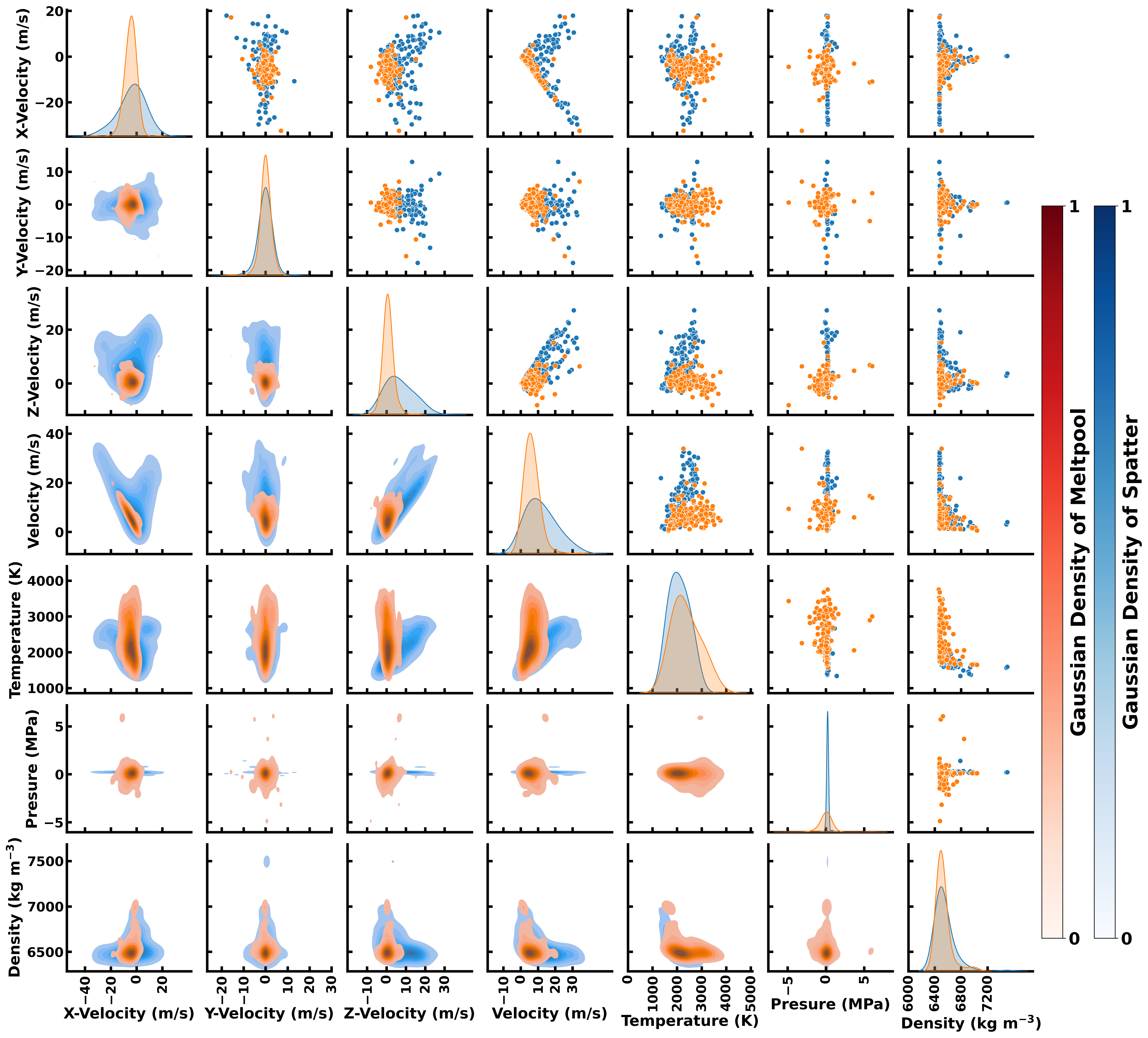
Figure 5: Pairplot correlating different measured properties of the meltpool and the spatter ejection through the histogram along the diagonal, Kernel Density Estimation (KDE) plots to the left of the diagonal and scatter plot to the right of the diagonal

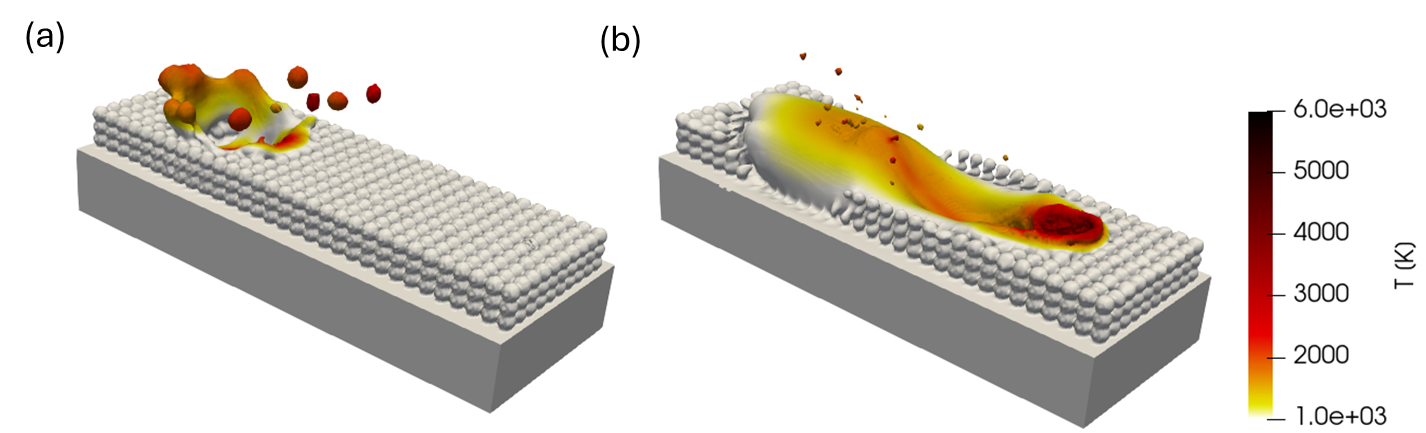
Figure 6: OpenFOAM simulation at 280 W and 1.5 m/s displaying spatter event at different timestep (a) spatter event 110 $\mu s$ (b) Spatter event at 440 $\mu s$

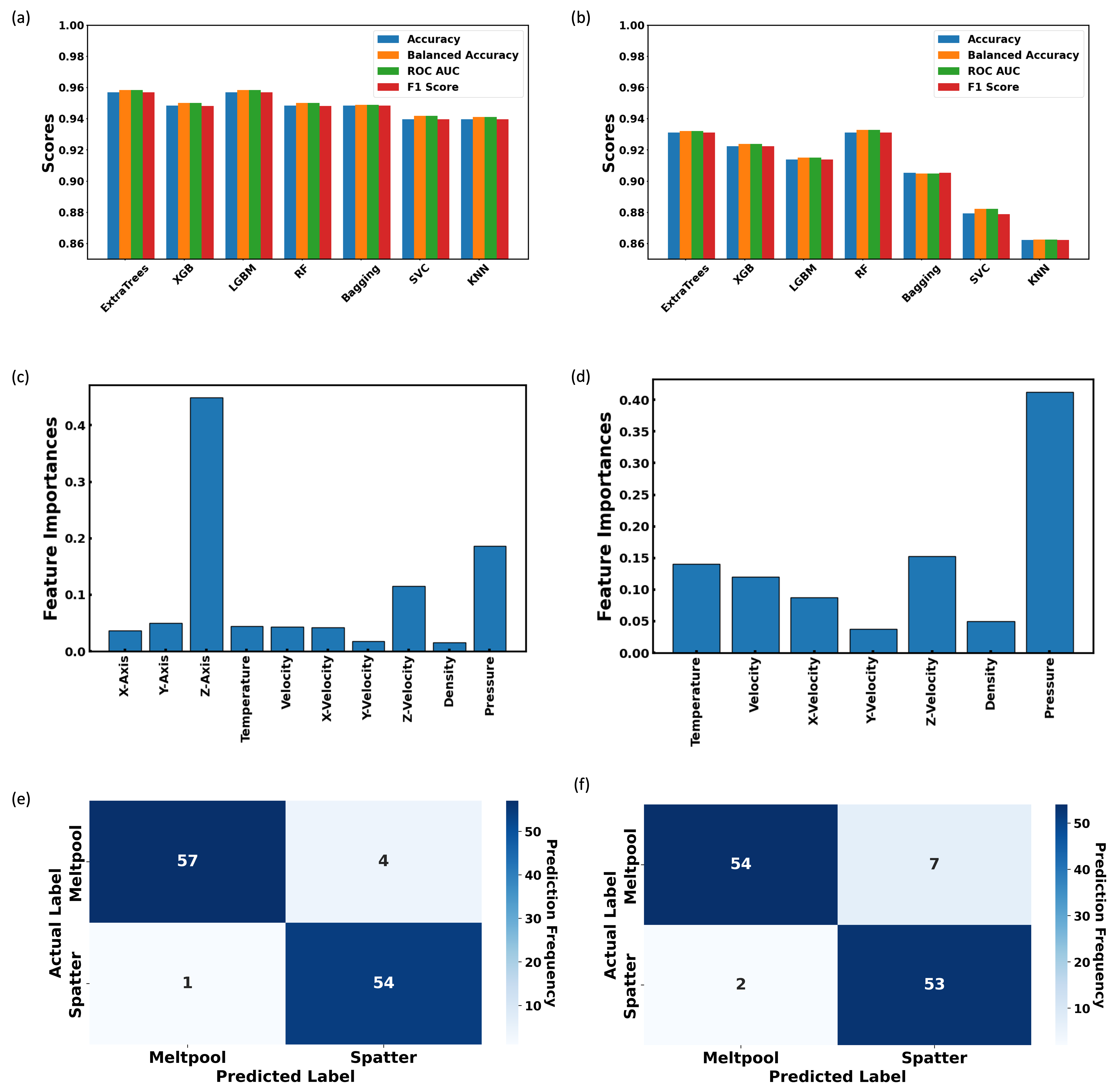
Figure 7: Performance measurement of ML models on classifying spatter ejection and meltpool with the following features: x-axis, y-axis, z-axis, temperature, velocity, x-velocity, y-velocity, z-velocity, density and pressure (a) Accuracy measurement of the spatter and meltpool classification using different ML models on OpenFOAM dataset with all the features (b) Accuracy measurement of the spatter and the meltpool classification while position components are excluded; tuning the input features to match that can be extracted from FLOW-3D for spatter ejection prediction (c) Feature importance measurement of all the input features into ML model (d) Feature importance measurement of the input features excluding position components into ML model (e) Quantification of the correct and wrong predictions of spatter and meltpool when all features were used (f) Quantification of the correct and wrong predictions of spatter and meltpool when all features were used excluding position components

3.2 Spatter and Meltpool Property Correlations

Meltpool dynamics relies on the process parameter, and spatter ejected from the meltpool can have properties close to the meltpool; however, it is unknown how close this properties can be due to unavailability of equipment that has the tolerance and sensitivity to detect the variations. Collecting measurements during the vapor plume generation from the meltpool further complicates the data extraction due to the poor visibility and short timescale between changing meltpool dynamics and spatter ejections. Harnessing the strength of high fidelity 3D simulation and ML models, the slight variation in the properties can appear in patterns across measurements and be detected; aiding in differentiating the measured properties of both the meltpool and the spatter at ejections. Informative statistical distribution was generated as shown in the Figure 4 and Figure 5. The diagonal of the pairplot displays a plotted histogram showing the distribution of the property measurements. On the left side of the diagonal, are the Kernel Density Estimation (KDE) plots showing the data density concentration while on the right-hand-side of the diagonal histogram are the scatter plots of the distribution. The histogram plots along the diagonal suggest that spatter has a wider spatial distribution, with its density spreading out over a larger range. Meltpool, on the other hand, shows a more concentrated spatial distribution, indicating a more localized phenomenon. Additionally, the wider distribution with respect to the spatial distributions (x, y, z) can be attributed to the possibility of the spatter ejection being detected within and away from the meltpool location as shown in the Figure 4 which can depend on ejection velocity and simulation’s timestep. The wider spatial distribution of the spatter is more prominent along the y-axis. The circular shape of the laser beam induces curvature growth of the meltpool, such that its breakage will lead to spatter detection in larger different between the magnitude of its standard deviation and the meltpool than what was observed for other axes. A wider separation was observed between the histogram plot of the meltpool and the spatter along the z-axis, and it can be attributed to the spatter ejection mostly occurring and detected at a higher height than the meltpool. For the velocity distributions as shown on Figure 5, except for y-velocity, the Spatter KDE plots, histogram and scatter plots are broader, suggesting a wider range of velocities, while the Meltpool plots are narrower, indicating more uniform velocities. y-velocity distributions appear to be similar with respect to the spatter and the meltpool, suggesting that y-velocity might be a weak parameter in driving spatter ejection. Also, density distributions between the spatter and the meltpool appear to be close to each other, with the spatter possessing slightly broader distribution to the upper end, indicating evidence of cooling. In general, spatter data points on the KDE plots, histogram and the scatter plots exhibit a wider spread, reinforcing the idea that spatter exhibits a greater variability in spatial and velocity distributions, while meltpool shows tighter clustering.

In contrast, wider distribution spreads were observed for the temperature and pressure of the meltpool in comparison to the spatter, implying a broader temperature and pressure range of the meltpool. Spatter shows higher peaks in the KDE plots, indicating temperatures are more consistent and concentrated around a mean value. The scatter plots for the spatter display more defined groupings, while the meltpool’s points are dispersed over a wider range, confirming the trends suggested by the KDE plots. Meltpool’s pressure distribution is wider also as indicated by its KDE plot, whereas spatter exhibits a sharper peak, suggesting a narrower range of pressure values is required for its ejections. The scatter plots corresponding to the pressure of the meltpool against other parameters show a more dispersed pattern. The wider temperature and pressure distribution of the meltpool dataset is due to the high gradients of these properties along the meltpool volume at a given timestep. Simultaneously, the narrower distribution of the spatter’s temperature and pressure in addition to it less concentration at the upper bound in comparison to the meltpool could be due to it ejection occurring away from the laser impact on the material and occurrence of cooling, which could depend on the offshoot velocity that will determine how far away it is from the laser. Overall, spatter represents a more variable and less controlled process with a broader range of values across most of the parameters, whereas meltpool indicates a more stable and consistent process where the parameters are more narrowly distributed around certain central values. Spatter ejection from the meltpool could be attributed to the locations in the meltpool that possess the observed magnitude or threshold for the combination of parameters. However, it is crucial to quantify these parameters based on their importance to spatter generation.

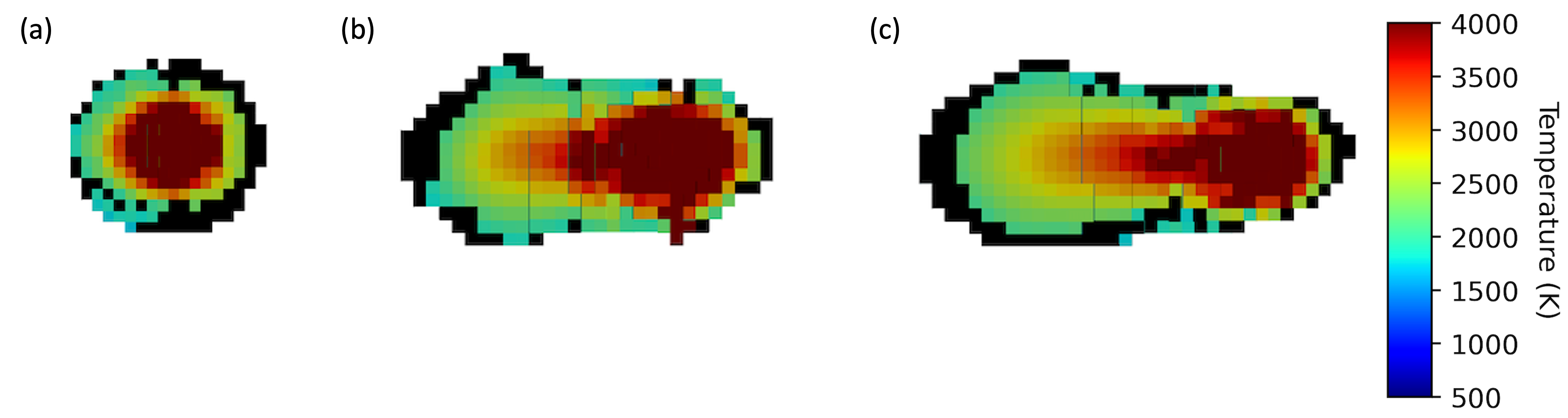
Figure 8: Spatter prediction on FLOW-3D simulation generated from testing FLOW-3D dataset on ML model that was trained using OpenFOAM. Region masked with black are identified as location predicted as spatter (a) prediction at timestep 65 $\mu s$ (b) prediction at timestep 165 $\mu s$ (c) prediction at timestep 265 $\mu s$.

3.3 Spatter and Meltpool Classification via ML Model

Classification task was conducted using the following ML models; Extremely Randomized Trees(ExtraTrees), Extreme Gradient Boosting(XGB), LGBM(Light Gradient Boosting Machine), RF(Random Forest), Bagging, Support Vector Classifier(SVC) and k-nearest neighbors(KNN). Our dataset was extracted from OpenFOAM simulation of two experiments at 545 W with scan speed of 2 m/s and 690 W and scan speed of 2 m/s. The dataset consists of 358 points whereby 50 % is spatter and the remaining 50 % is associated with the meltpool. The train-test split used is 70 %-30 %. Upon screening different ML models, where the collected features include x-axis, y-axis, z-axis, temperature, velocity, x-velocity, y-velocity, z-velocity, density and pressure, high accuracy were observed for all the ML models, with ExtraTrees being the highest at 96 % and KNN being the lowest at 94 % as shown on the figure 7a. The importance of the features used in ML testing, as shown on the Figure 7b, followed the trend: z-axis $>$ pressure $>$ z-velocity $>$ y-axis $>$ temperature $>$ velocity $>$ x-velocity $>$ y-velocity $>$ density. The highest contribution of the z-axis to the accuracy is attributed to the wide separation observed between the spatter and the meltpool when z-axis is paired together with itself, or other parameters as shown on the histogram, KDE, and scatter plots as shown on Figure 4.

The methodologies of our data extraction and combination of parameters for this classification task is promising. These techniques can serve as a benchmark in predicting spatter or developing reduced order model package for spatter generation either with desired simulation packages or collected experimental measurements. Consequently, the high accuracy outcome of ML predictions underscore the efficacy of our ML models in predicting spatter events on the commercial software package, FLOW-3D, which lacks the capability to accurately simulate spatter. Therefore, modelling LPBF in FLOW-3D generates a dataset that is specifically for the meltpool with no spatter occurrence. Although some locations in the meltpool dataset generated by the FLOW-3D could be having spatter-like properties or the property-threshold required for spatter ejection, but rather remain in the meltpool due to the absence of physics module required to resolve the mass transfer between the interface of the different phases. Therefore, adapting the current ML model that was trained on OpenFOAM dataset will necessitate removal of spatial components (x, y, z) from the features that will be used to train and test ML models. On training and testing OpenFOAM dataset without spatial components, high accuracies were still achieved with slight decrease. Both ExtraTrees and RF exhibit highest values at 93 % while KNN has the lowest value of 86 % as shown in Figure 7b. It was noted that RF changed the least by 0.9 %, while ExtraTrees changed by 1.7 % and KNN changed the most by 8 % as compared to their respective initial accuracy that were achieved with spatial component being included in the features. Consequently, RF was chosen for predicting spatter on FLOW-3D software due to its best stability as it demonstrated least changes with different feature configurations. The trend observed in the feature importance studies without spatial components, as shown in Figure 7d follows the trend of pressure $>$ z-velocity $>$ temperature $>$ velocity $>$ x-velocity $>$ y-velocity $>$ density. Evidently, pressure is not only the most significant parameter driving the dynamics in the meltpool, but also dictates possibility of spatter ejection as its magnitude is confined within a narrow range as shown in Figure 5. Strong importance observed with respect to z-velocity can be understood from the tendency of a body that possesses high z-velocity to travel upward, and we observed a narrow range for meltpool z-velocity, which is a subset of spatter’s z-velocity. Also, observing temperature having less importance than the z-velocity despite its direct relationship with pressure according to Clausius–Clapeyron relation could be attributed to the saturation that is reached such that increment in the temperature will result in boiling of the material which will not lead to spatter ejection, but more plume generation. High contribution of z-velocity to the spatter ejection could also be understood from the parabolic shape of the meltpool which is formed as the laser traverse in x-axis direction. Hot fluid will build up in the direction of the laser, which can break up to create spatter due to its elongation as shown in figure 6a, via shear thinning. Additionally, spatter breakage can further intensify the backward dispersion of material and energy that are in form of a wave which can travel through the high gradient region of the meltpool, creating z-velocity component that could enhance ejection. The backward dispersion of material and energy in the meltpool can be attributed to the combination of other factors such as pressure, temperature gradient, and the vibration in the meltpool which can also influence other properties like viscosity and surface tension to cause Marangoni effect and promote meltpool flow, elongation and ultimately fluid ejections.

To gain further insight to the distribution of ML model predictions, we constructed a precision recall table as shown on Figure 7e and 7f for predictions with spatial components included in the features and with no spatial components respectively. We observed our model having the capability in predicting most of the points with the meltpool and the spatter. The most wrong prediction observation for the model with the presence of spatial component features and non-spatial component features is associated with regions that were meltpool but rather predicted as spatter. Upon testing our model on FLOW-3D, voxels that matches the property of spatter were identified and masked with black points as shown on Figure 8. At the early timestep of the FLOW-3D simulation, spatter predictions were predominantly observed at the front of the meltpool (Figure 8a), then at the latter timesteps (Figure 8a and the 8b), spatter tends to occupy the backward side of the meltpool, this is similar to observed OpenFOAM simulation for spatter generation as shown in Figure 6. It should be noted that conditions for spatter generation were not met at the location of the hotspot of the meltpool due to the high temperature that could be causing fluid evaporation. Consequently, the high accuracy outcome of RF underscores the efficacy of our developed methodology for the reduced-order task on spatter prediction whereby testing datasets of different process parameters generated from commercial software, FLOW-3D towards development of process map is possible.

3.4 Spatter Process Map

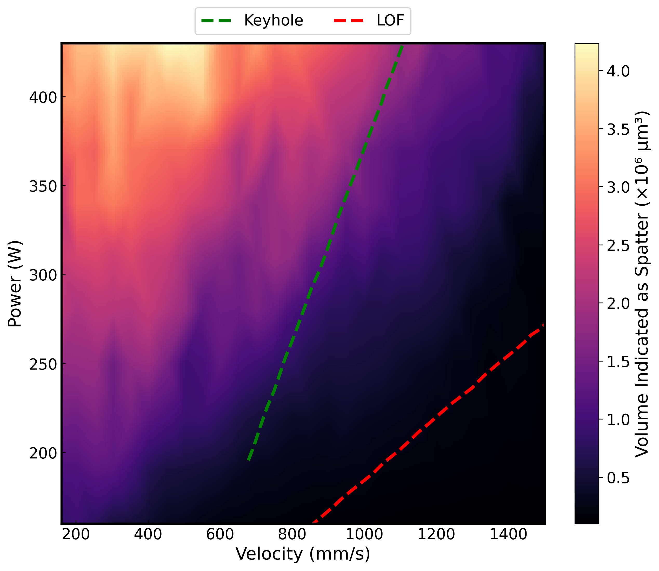
Figure 9: Process map generated via hybrid of OpenFOAM trained ML model on FLOW-3D dataset to understand relationship between spatter formation and process conditions. The process map was created using 283 FLOW-3D simulations with different combinations of power and velocity

Display of spatter quantification with varying power/velocity combination will provide access to suitable operating window with minimal defects for producing part. Running openFOAM for additive manufacturing is computationally expensive due to many physics it is configured to solve as compared to FLOW-3D, a devoted package for AM, but lacks physics to solve spatter generation. On the same machine, FLOW-3D is 100 times faster than OpenFOAM in generating LPBF solution. Building hybrid of OpenFOAM and FLOW-3D via the high accuracy ML model as a reduced order model is attractive for large dataset generation for the development of spatter process map. As shown in Figure 9, the spatter quantification follows a predictable trend within processing parameter space for laser LPBF. It was observed that more spatter was generated at high power low velocity which is the region observed for keyhole formation in porosity. At low power and high speed, less spatter was observed and this can be associated with the region know as lack of fusion [12]. The reason for the less spatter at this region can be attributed to less interaction of the material and the laser, creating less melting resulting in the melt track that will not be fully join. Based on the operating conditions, we observed the trend follow by the quantity of spatter generation as high power/low speed $>$ high power/high speed $>$ low power/low speed $>$ low power/high speed. Safe operating window lies between the region of lack of fusion and keyhole. Although the safe operating might possess slightly more spatter than the lack of fusion region, however as it has been previous studied than operating at this region prevents defects associated with porosity, additionally machine improved design or shielding gas flow could aid spatter elimination while operating within the safe operating window.

4 Conclusion

In this work, we developed multiphysics simulation of a single-track selective laser melting using OpenFOAM, which has the capability to produce the 3D high resolution properties of spatter and meltpool dynamics. In addition, tracking algorithm was developed to extract the dataset used to characterize spatter ejection, the meltpool, and to perform ML classification tasks. Upon screening our datasets using different machine learning models such as ExtraTrees, XGB, LGBM, RF, Bagging, SVC and KNN, we observed high accuracy greater than 93 % for all the ML models implemented with the highest being ExtraTrees and the lowest being KNN. Upon removing spatial component (x, y, z) from the OpenFOAM dataset used to train/test ML model so as to match the accessible dataset that can be extracted from FLOW-3D, we found ExtraTrees and Random Forest to exhibit highest values at 93 % while KNN has the lowest value of 86 %. Random Forest shows least changes of 0.9 % when compared to their respective initial accuracy that was achieved with spatial component being included in the features. High accuracy outcome of ML predictions underscore the efficacy of our ML models in exploring the model for the reduced-order task of spatter prediction, by rigorously testing datasets from the commercial software. Region association with spatter on FLOW-3D software was predicted and identified as voxel. Simulating additive manufacturing process is 100 times faster on FLOW-3D than OpenFOAM, making screening of 281 different process parameters collected from FLOW-3D a feasible path towards developing a process map using ML model trained on OpenFOAM dataset a means of displaying spatter trend in large process parameter space. Correlation of the possible amount of spatter with changing power/velocity combination was generated. It was observed that at a high power and low laser speed, more spatters were generated in comparison to low power and high speed.

Declarations

Funding

Research was sponsored by the Army Research Laboratory and was accomplished under Cooperative Agreement Number W911NF-20-2-0175. The views and conclusions contained in this document are those of the authors and should not be interpreted as representing the official policies, either expressed or implied, of the Army Research Laboratory or the U.S. Government. The U.S. Government is authorized to reproduce and distribute reprints for Government purposes notwithstanding any copyright notation herein.

Competing Interests

The authors have no competing interests to declare that are relevant to the content of this article.

Appendix A OpenFOAM simulation domain

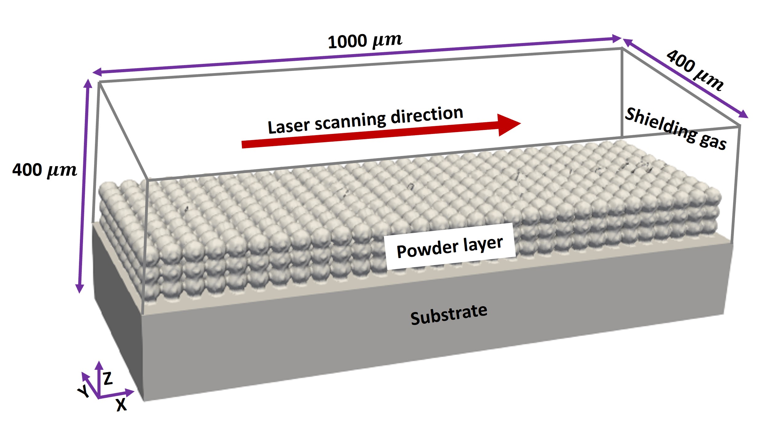
Figure 10: Schematic illustration of the computational domain with random packing of Stainless steel powder bed

Table 3: Physical properties and related coefficients of SST in the simulation with subscript s for solid phase, l for liquid, v for vapor and a for the shielding gas argon.

Parameter	Value	Units
Liquidus temperature, $\rho$, 298 K	7950	kg/m3
Evaporation Temperature, $\rho$, 1923 K	6765	kg/m3
Surface tension liquid, $C_{v}$, 298 K	470	J/kg/K
Specific heat solid, $C_{v}$, 1923 K	1873	J/kg/K
Specific heat liquid, $C_{v,vapor}$	449	J/kg/K
Specific heat vapor, $k$, 298 K	13.4	W/m/K
Specific heat nitrogen, $k$, 1923 K	30.5	W/m/K
Thermal conductivity solid, $\eta$	0.008	kg/m/s
Thermal conductivity liquid, $\sigma$	1.882	$kg/s^{2}$
Heat of fusion, $T_{L}$	1723	K
Heat of evaporation, $T_{S}$	1658	K
Dynamic viscosity liquid, $\epsilon$	0.15	-
Dynamic viscosity vapor, $a$	0.25	-
Prandtl number liquid, $\Delta H_{f}$	2.6 $\times 10^{5}$	J/kg
Prandtl number vapor, $\Delta H_{v}$	7.45 $\times 10^{6}$	J/kg
Absorptivity, $a$	0.25	-

References

- [1] Florian Wirth, Teresa Tonn, Markus Schöberl, Stefan Hermann, Hannes Birkhofer, and Vasily Ploshikhin. Implementation of the marangoni effect in an open-source software environment and the influence of surface tension modeling in the mushy region in laser powder bed fusion (lpbf). Modelling and Simulation in Materials Science and Engineering, 30(3):034001, 2022.
- [2] Giulia Repossini, Vittorio Laguzza, Marco Grasso, and Bianca Maria Colosimo. On the use of spatter signature for in-situ monitoring of laser powder bed fusion. Additive Manufacturing, 16:35–48, 2017.
- [3] Ross Cunningham, Sneha P Narra, Colt Montgomery, Jack Beuth, and AD Rollett. Synchrotron-based x-ray microtomography characterization of the effect of processing variables on porosity formation in laser power-bed additive manufacturing of ti-6al-4v. Jom, 69:479–484, 2017.
- [4] Chinnapat Panwisawas, Yuanbo T Tang, and Roger C Reed. Metal 3d printing as a disruptive technology for superalloys. Nature Communications, 11(1):2327, 2020.
- [5] Jie Yin, Dengzhi Wang, Liangliang Yang, Huiliang Wei, Peng Dong, Linda Ke, Guoqing Wang, Haihong Zhu, and Xiaoyan Zeng. Correlation between forming quality and spatter dynamics in laser powder bed fusion. Additive Manufacturing, 31:100958, 2020.
- [6] Zheng Li, Hao Li, Jie Yin, Yan Li, Zhenguo Nie, Xiangyou Li, Deyong You, Kai Guan, Wei Duan, Longchao Cao, et al. A review of spatter in laser powder bed fusion additive manufacturing: In situ detection, generation, effects, and countermeasures. Micromachines, 13(8):1366, 2022.
- [7] S Mohammad H Hojjatzadeh, Niranjan D Parab, Qilin Guo, Minglei Qu, Lianghua Xiong, Cang Zhao, Luis I Escano, Kamel Fezzaa, Wes Everhart, Tao Sun, et al. Direct observation of pore formation mechanisms during lpbf additive manufacturing process and high energy density laser welding. International Journal of Machine Tools and Manufacture, 153:103555, 2020.
- [8] Aiden A Martin, Nicholas P Calta, Saad A Khairallah, Jenny Wang, Phillip J Depond, Anthony Y Fong, Vivek Thampy, Gabe M Guss, Andrew M Kiss, Kevin H Stone, et al. Dynamics of pore formation during laser powder bed fusion additive manufacturing. Nature communications, 10(1):1987, 2019.
- [9] T Mukherjee and Tarasankar DebRoy. Mitigation of lack of fusion defects in powder bed fusion additive manufacturing. Journal of Manufacturing Processes, 36:442–449, 2018.
- [10] Patcharapit Promoppatum, Raghavan Srinivasan, Siu Sin Quek, Sabeur Msolli, Shashwat Shukla, Nur Syafiqah Johan, Sjoerd van der Veen, and Mark Hyunpong Jhon. Quantification and prediction of lack-of-fusion porosity in the high porosity regime during laser powder bed fusion of ti-6al-4v. Journal of Materials Processing Technology, 300:117426, 2022.
- [11] Zhongshu Ren, Lin Gao, Samuel J Clark, Kamel Fezzaa, Pavel Shevchenko, Ann Choi, Wes Everhart, Anthony D Rollett, Lianyi Chen, and Tao Sun. Machine learning–aided real-time detection of keyhole pore generation in laser powder bed fusion. Science, 379(6627):89–94, 2023.
- [12] Jerard V Gordon, Sneha P Narra, Ross W Cunningham, He Liu, Hangman Chen, Robert M Suter, Jack L Beuth, and Anthony D Rollett. Defect structure process maps for laser powder bed fusion additive manufacturing. Additive Manufacturing, 36:101552, 2020.
- [13] Zachary A Young, Qilin Guo, Niranjan D Parab, Cang Zhao, Minglei Qu, Luis I Escano, Kamel Fezzaa, Wes Everhart, Tao Sun, and Lianyi Chen. Types of spatter and their features and formation mechanisms in laser powder bed fusion additive manufacturing process. Additive Manufacturing, 36:101438, 2020.
- [14] Ahmad Bin Anwar and Quang-Cuong Pham. Study of the spatter distribution on the powder bed during selective laser melting. Additive Manufacturing, 22:86–97, 2018.
- [15] Zhiqiang Wang, Xuede Wang, Xin Zhou, Guangzhao Ye, Xing Cheng, and Peiyu Zhang. Investigation into spatter particles and their effect on the formation quality during selective laser melting processes. CMES-Computer Modeling in Engineering & Sciences, 124(1), 2020.
- [16] Shuhao Wang, Jinsheng Ning, Lida Zhu, Zhichao Yang, Wentao Yan, Yichao Dun, Pengsheng Xue, Peihua Xu, Susmita Bose, and Amit Bandyopadhyay. Role of porosity defects in metal 3d printing: Formation mechanisms, impacts on properties and mitigation strategies. Materials Today, 2022.
- [17] Sonny Ly, Alexander M Rubenchik, Saad A Khairallah, Gabe Guss, and Manyalibo J Matthews. Metal vapor micro-jet controls material redistribution in laser powder bed fusion additive manufacturing. Scientific reports, 7(1):4085, 2017.
- [18] Florian Wirth, Alex Frauchiger, Kai Gutknecht, and Michael Cloots. Influence of the inert gas flow on the laser powder bed fusion (lpbf) process. In Industrializing Additive Manufacturing: Proceedings of AMPA2020, pages 192–204. Springer, 2021.
- [19] Christopher Barrett, Carolyn Carradero, Evan Harris, Jeremy McKnight, Jason Walker, Eric MacDonald, and Brett Conner. Low cost, high speed stereovision for spatter tracking in laser powder bed fusion. In 2018 International Solid Freeform Fabrication Symposium. University of Texas at Austin, 2018.
- [20] Nicholas O’Brien, Syed Zia Uddin, Jordan Weaver, Jake Jones, Satbir Singh, and Jack Beuth. Computational analysis and experiments of spatter transport in a laser powder bed fusion machine. Additive Manufacturing, page 104133, 2024.
- [21] Christopher Barrett, Carolyn Carradero, Evan Harris, Kirk Rogers, Eric MacDonald, and Brett Conner. Statistical analysis of spatter velocity with high-speed stereovision in laser powder bed fusion. Progress in Additive Manufacturing, 4(4):423–430, 2019.
- [22] Hiroshi Nakamura, Yousuke Kawahito, Koji Nishimoto, and Seiji Katayama. Elucidation of melt flows and spatter formation mechanisms during high power laser welding of pure titanium. Journal of Laser Applications, 27(3), 2015.
- [23] Minglei Qu, Qilin Guo, Luis I Escano, Ali Nabaa, S Mohammad H Hojjatzadeh, Zachary A Young, and Lianyi Chen. Controlling process instability for defect lean metal additive manufacturing. Nature communications, 13(1):1079, 2022.
- [24] Shengjie Deng, Hui-Ping Wang, Fenggui Lu, Joshua Solomon, and Blair E Carlson. Investigation of spatter occurrence in remote laser spiral welding of zinc-coated steels. International Journal of Heat and Mass Transfer, 140:269–280, 2019.
- [25] OpenCFD Ltd (ESI Group). Openfoam documentation. (online) https://www.openfoam.com/documentation/overview).
- [26] OpenCFD Ltd (ESI Group). Openfoam news. (online) https://www.openfoam.com/news/main-news/openfoam-v20-12).
- [27] Francis Ogoke, William Lee, Ning-Yu Kao, Alexander Myers, Jack Beuth, Jonathan Malen, and Amir Barati Farimani. Convolutional neural networks for melt depth prediction and visualization in laser powder bed fusion. The International Journal of Advanced Manufacturing Technology, 129(7):3047–3062, 2023.
- [28] Odinakachukwu Francis Ogoke, Kyle Johnson, Michael Glinsky, Chris Laursen, Sharlotte Kramer, and Amir Barati Farimani. Deep-learned generators of porosity distributions produced during metal additive manufacturing. Additive Manufacturing, 60:103250, 2022.
- [29] Francis Ogoke and Amir Barati Farimani. Thermal control of laser powder bed fusion using deep reinforcement learning. Additive Manufacturing, 46:102033, 2021.
- [30] Parand Akbari, Francis Ogoke, Ning-Yu Kao, Kazem Meidani, Chun-Yu Yeh, William Lee, and Amir Barati Farimani. Meltpoolnet: Melt pool characteristic prediction in metal additive manufacturing using machine learning. Additive Manufacturing, 55:102817, 2022.
- [31] XIA Yang, Suhaib Zafar, J-X Wang, and Heng Xiao. Predictive large-eddy-simulation wall modeling via physics-informed neural networks. Physical Review Fluids, 4(3):034602, 2019.
- [32] Francis Ogoke, Quanliang Liu, Olabode Ajenifujah, Alexander Myers, Guadalupe Quirarte, Jack Beuth, Jonathan Malen, and Amir Barati Farimani. Inexpensive high fidelity melt pool models in additive manufacturing using generative deep diffusion. arXiv preprint arXiv:2311.16168, 2023.
- [33] Chengcheng Wang, XP Tan, Shu Beng Tor, and CS Lim. Machine learning in additive manufacturing: State-of-the-art and perspectives. Additive Manufacturing, 36:101538, 2020.
- [34] Emmanuel Stathatos and George-Christopher Vosniakos. Real-time simulation for long paths in laser-based additive manufacturing: a machine learning approach. The International Journal of Advanced Manufacturing Technology, 104:1967–1984, 2019.
- [35] Yayati Jadhav, Joseph Berthel, Chunshan Hu, Rahul Panat, Jack Beuth, and Amir Barati Farimani. Stressd: 2d stress estimation using denoising diffusion model. Computer Methods in Applied Mechanics and Engineering, 416:116343, 2023.
- [36] Sofia Sheikh, Brent Vela, Vahid Attari, Xueqin Huang, Peter Morcos, James Hanagan, Cafer Acemi, Ibrahim Karaman, Alaa Elwany, and Raymundo Arroyave´. Exploring chemistry and additive manufacturing design spaces: a perspective on computationally-guided design of printable alloys. Materials Research Letters, 12(4):235–263, 2024.
- [37] Xiling Yao, Seung Ki Moon, and Guijun Bi. A hybrid machine learning approach for additive manufacturing design feature recommendation. Rapid Prototyping Journal, 23(6):983–997, 2017.
- [38] Martin P Bendsoe, Erik Lund, Niels Olhoff, and Ole Sigmund. Topology optimization-broadening the areas of application. Control and Cybernetics, 34(1):7–35, 2005.
- [39] AmirPouya Hemmasian, Francis Ogoke, Parand Akbari, Jonathan Malen, Jack Beuth, and Amir Barati Farimani. Surrogate modeling of melt pool temperature field using deep learning. Additive Manufacturing Letters, 5:100123, 2023.
- [40] Yang Du, Tuhin Mukherjee, and Tarasankar DebRoy. Physics-informed machine learning and mechanistic modeling of additive manufacturing to reduce defects. Applied Materials Today, 24:101123, 2021.
- [41] Jennifer Lundkvist. Cfd simulation of fluid flow during laser metal wire deposition using openfoam: 3d printing, 2019.
- [42] J U Brackbill, D B Kothe, and C Zemach. A continuum method for modeling surface tension. J. Comput. Phys., 100:335–354, 1992.
- [43] Mohammad Bahreini, Abbas Ramiar, and Ali Akbar Ranjbar. Development of a phase change model for volume-of-fluid method in openfoam. Journal of Heat and Mass Transfer Research, 3(2):131–143, 2016.
- [44] Wen Ho Lee. A pressure iteration scheme for two-phase flow modeling. Multiphase transport fundamentals, reactor safety, applications, 1:407–431, 1980.
- [45] NL Scuro, M Poschmann, O Beneš, and MHA Piro. Progress in coupling computational thermodynamics and computational fluid dynamics to support molten salt reactor applications. In Conference Paper: G4SR4, pages 1–15, 2022.
- [46] Pierre Geurts, Damien Ernst, and Louis Wehenkel. Extremely randomized trees. Machine learning, 63(1):3–42, 2006.
- [47] Tianqi Chen and Carlos Guestrin. Xgboost: A scalable tree boosting system. In Proceedings of the 22nd acm sigkdd international conference on knowledge discovery and data mining, pages 785–794, 2016.
- [48] Guolin Ke, Qi Meng, Thomas Finley, Taifeng Wang, Wei Chen, Weidong Ma, Qiwei Ye, and Tie-Yan Liu. Lightgbm: A highly efficient gradient boosting decision tree. In Advances in neural information processing systems, pages 3146–3154, 2017.
- [49] Leo Breiman. Random forests. Machine learning, 45(1):5–32, 2001.
- [50] Leo Breiman. Bagging predictors. Machine learning, 24(2):123–140, 1996.
- [51] Corinna Cortes and Vladimir Vapnik. Support-vector networks. Machine learning, 20(3):273–297, 1995.
- [52] Alexander J Myers, Guadalupe Quirarte, Francis Ogoke, Brandon M Lane, Syed Zia Uddin, Amir Barati Farimani, Jack L Beuth, and Jonathan A Malen. High-resolution melt pool thermal imaging for metals additive manufacturing using the two-color method with a color camera. Additive Manufacturing, 73:103663, 2023.
- [53] Christophe Fiorio and Jens Gustedt. Two linear time union-find strategies for image processing. Theoretical Computer Science, 154(2):165–181, 1996.