Synthetic Tabular Data Validation: A Divergence-Based Approach

Abstract

The ever-increasing use of generative models in various fields where tabular data is used highlights the need for robust and standardized validation metrics to assess the similarity between real and synthetic data. Current methods lack a unified framework and rely on diverse and often inconclusive statistical measures. Divergences, which quantify discrepancies between data distributions, offer a promising avenue for validation. However, traditional approaches calculate divergences independently for each feature due to the complexity of joint distribution modeling. This paper addresses this challenge by proposing a novel approach that uses divergence estimation to overcome the limitations of marginal comparisons. Our core contribution lies in applying a divergence estimator to build a validation metric considering the joint distribution of real and synthetic data. We leverage a probabilistic classifier to approximate the density ratio between datasets, allowing the capture of complex relationships. We specifically calculate two divergences: the well-known Kullback-Leibler (KL) divergence and the Jensen-Shannon (JS) divergence. KL divergence offers an established use in the field, while JS divergence is symmetric and bounded, providing a reliable metric. The efficacy of this approach is demonstrated through a series of experiments with varying distribution complexities. The initial phase involves comparing estimated divergences with analytical solutions for simple distributions, setting a benchmark for accuracy. Finally, we validate our method on a real-world dataset and its corresponding synthetic counterpart, showcasing its effectiveness in practical applications. This research offers a significant contribution with applicability beyond tabular data and the potential to improve synthetic data validation in various fields.

Keywords Divergence  $\cdot$ Kullback-Leibler  $\cdot$ Jensen-Shannon  $\cdot$ Synthetic Data Generation  $\cdot$ Tabular Data  $\cdot$ Validation  $\cdot$ Density Ratio

1 Introduction

Generative models (GMs) are emerging as a disruptive force within artificial intelligence. By learning the underlying patterns and distributions of real-world data, these models can create novel synthetic data replicating the characteristics of the original domain. These synthetic data offer significant advantages for various research and development applications. In particular, synthetic data can be used for data augmentation, addressing limitations in data collection efforts. In addition, it can ensure privacy protection by replacing sensitive real-world information. Furthermore, it facilitates the exploration of rare or extreme scenarios (edge cases) that might be difficult or expensive to encounter in real-world settings. As a result, the synthetic data generated by these models is accelerating innovation in various fields, including healthcare[1], finance[2], and the development of autonomous vehicles[3], to mention some.

Following the impressive advances in GMs for data generation, a critical aspect emerges: ensuring the quality and effectiveness of synthetic data. Replicating statistical properties, accuracy, consistency, and domain-specific relevance of the source data is essential. This challenge becomes especially pronounced as GMs gain traction within engineering design communities. The need for robust and standardized validation metrics becomes paramount. The current literature highlights a significant gap in this area. Although there are standardized evaluation metrics for the generation of synthetic images [4], [5], and the generation of text [6], [7], measuring the quality of synthetic tabular data presents unique challenges. Unlike image data, qualitative evaluation through visual inspection is not feasible. Additionally, relying solely on expert insight can be highly inefficient. The existing landscape for tabular data validation often focuses primarily on the efficacy or utility in machine learning tasks [8][9]. However, a consistent approach to assess the similarity between synthetic and real tabular data remains sparse. Studies employ a diverse set of metrics, including pairwise correlation difference[10], support coverage[11], likelihood fitness[12], alongside various statistic values[13],[14]. Reviews such as [15] attempt to categorize these techniques, but a truly standardized approach or a single metric that captures the full spectrum of statistical information from a distribution remains a challenge.

This paper aims to address this gap by proposing a divergence estimator. Divergences offer a comprehensive approach to the validation of similarity. These measures quantify the discrepancy between two probability distributions, effectively capturing the differences between real and synthetic data. Unlike traditional methods that often focus on individual attributes [16][17], divergences can consider the joint distribution of all attributes, providing a more holistic view of the data. However, it is important to acknowledge the challenge associated with joint distributions. Modeling the intricate relationships between all features in a dataset can be computationally expensive and intractable. Although some existing papers explore divergences or distances for validation, they often apply them to single attributes because of this limitation [11][18][19]. Crucially, even if individual features appear similar, the joint distribution, which captures the relationships between them, may differ significantly [20]. This underscores the importance of considering the joint distribution for accurate assessment. Our proposed divergence estimator addresses this challenge by offering a way to efficiently capture these complex joint distributions. This allows us to compute divergences between real and synthetic data, enabling a more comprehensive and robust evaluation of synthetic data quality. The advantages of using divergences for validation remain the same:

• Sensitivity to Complex Distributions: Divergences can capture the full complexity of real-world data distributions, including nonlinear relationships and rare events, which traditional methods might miss.

• Robustness to Noise: Divergences are less sensitive to noise and outliers, making them more reliable for practical applications.

• Interpretability: Divergences can be easily interpreted and visualized, providing valuable insights into the discrepancies between real and synthetic data.

Therefore, we introduce a novel methodology to validate real and synthetic data similarity:

• Divergence-based Similarity Estimation: Our approach leverages divergence estimation to quantify the discrepancy between the joint probability distributions of real and synthetic tabular data. This approach goes beyond traditional validation metrics, which often focus on marginal statistics.

• Probabilistic Discriminator Network for Density Ratio Estimation: To facilitate divergence calculations, we introduce an innovative approximation technique based on a probabilistic discriminator network [21]. This network plays a crucial role in estimating the density ratio between real and synthetic distributions, which forms the basis for divergence computations.

• KL Divergence and JS Divergence for Validation: We acknowledge the widespread use of Kullback-Leibler (KL) divergence in information theory (often referred to as relative entropy) for divergence calculations. However, we recognize its limitations: KL divergence is not a true distance in terms of mathematics [22] due to its asymmetry and the potential for infinite values in certain scenarios. To address this, we propose the inclusion of the Jensen-Shannon (JS) divergence, which offers desirable properties of being bounded and symmetric, thus defining a proper distance metric. This bounded metric is crucial to assess the quality of synthetic data generation.

• Rigorous Evaluation Framework: We introduce a comprehensive evaluation framework to assess the efficacy of our proposed method. We initially apply our method to simple distributions where analytical solutions for divergences exist. This serves as a benchmark to validate the accuracy of our estimated divergences. Following the initial validation, we progress to more complex scenarios and finally apply our method to real-world datasets and their corresponding synthetically generated counterparts. This allows us to assess the effectiveness of our approach in practical applications.

• Broad Applicability: Due to the adaptability of our divergence-based validation method, it can be applied to various types of data beyond tabular formats. This has the potential to significantly impact numerous fields such as healthcare, finance, and manufacturing. The adoption of our approach can lead to substantial improvements in the accuracy and reliability of synthetic data validation in various domains.

2 Background

2.1 Divergence definition

Let us consider two probability distributions, $p(x)$ and $q(x)$, for a random variable $x$. In the context of probability distributions, divergence quantifies the dissimilarity between $p(x)$ and $q(x)$. In essence, it measures how different these distributions are in terms of the probabilities they assign to each possible value of $x$. Divergences play a crucial role in various fields, including Machine Learning (ML), as they provide a way to compare and analyze the behavior of different probability distributions.

The Kullback-Leibler divergence is a common measure in information theory to quantify the discrepancy between $p(x)$ and $q(x)$. Denoted $D_{\mathbb{KL}}\big{(}p(x)\|q(x)\big{)}$, the KL divergence captures the asymmetry of this difference by measuring the expected penalty incurred by assuming $q(x)$ to be an approximation of the true distribution $p(x)$. Due to its extensive applicability in various fields, the KL divergence remains a dominant metric for comparing probability distributions. The KL divergence between $p(x)$ and $q(x)$ is given by

$$D_{\mathbb{KL}}\big{(}p(x)\|q(x)\big{)}=\int p(x)\log\frac{p(x)}{q(x)}dx.$$ (1)

Unfortunately, this expression is usually intractable. Thus, we must approximate it using Monte Carlo (MC) simulation, assuming we can draw $L$ samples from $p(x)$:

$$\int p(x)\log\frac{p(x)}{q(x)}dx\approx\frac{1}{L}\sum_{i=1}^{L}\log\frac{p\left(x_{i}\right)}{q\left(x_{i}\right)},\quad x_{i}\sim p(x).$$ (2)

To create a symmetric and bounded measure of divergence between $p(x)$ and $q(x)$, the Jensen-Shannon divergence is based on the KL divergence. The JS divergence denoted $D_{\mathbb{JS}}\big{(}p(x)\|q\big{(}x))\big{)}$, is a true distance defined as the KL average between both distributions and a common reference:

$$D_{\mathbb{JS}}\big{(}p(x)\|q(x)\big{)}=\frac{1}{2}D_{\mathbb{KL}}\big{(}p(x)\|m(x)\big{)}+\frac{1}{2}D_{\mathbb{KL}}\big{(}q(x)\|m(x)\big{)}.$$ (3)

The common reference distribution, $m(x)$, is typically chosen as the midpoint between the two original distributions, such as the average: $m(x)=\big{(}p(x)+q(x)\big{)}/2$. Importantly, the JS divergence is inherently bounded. When employing a base-$2$ logarithm, the maximum divergence value is $1$.

Similarly to KL, the JS divergence can also be estimated using MC simulation:

$$D_{\mathbb{JS}}\big{(}p(x)\|q(x)\big{)}$$ (4)

$$\approx\frac{1}{2L}\sum_{i=1}^{L}\log\frac{p\left(x_{i}\right)}{m\left(x_{i}\right)}+\frac{1}{2L}\sum_{i=1}^{L}\log\frac{q\left(\tilde{x}_{i}\right)}{m\left(\tilde{x}_{i}\right)}=\frac{1}{2L}\sum_{i=1}^{L}\log\left(\frac{2p\left(x_{i}\right)}{p\left(x_{i}\right)+q\left(x_{i}\right)}\right)+\frac{1}{2L}\sum_{i=1}^{L}\log\left(\frac{2q\left(\tilde{x}_{i}\right)}{p\left(\tilde{x}_{i}\right)+q\left(\tilde{x}_{i}\right)}\right),$$

assuming that we can generate $L$ samples from both distributions

$$\left\{\begin{array}[]{l}x_{i}\sim p(x)\\ \tilde{x}_{i}\sim q(x)\end{array}\right..$$ (5)

2.2 Estimating density ratio using probabilistic classification

Density ratio estimation focuses on estimating the ratio $r^{*}(x)$ of two probability densities, $p(x)$ and $q(x)$, based solely on samples drawn from these distributions. The ratio is therefore defined as

$$r^{*}(x)=\frac{p(x)}{q(x)},$$ (6)

where $*$ refers to the exact value. This approach avoids directly estimating individual densities since any errors in the denominator (i.e., $q(x)$) are dramatically amplified during the ratio calculation. The classical probabilistic classification approach remains popular among the various methods of estimating the density ratio due to its relative simplicity. This subsection reviews the method described by [21] for estimating the KL divergence. We further demonstrate its application to the JS divergence estimation as well.

Estimating (1) and (3) is based on determining the unknown density ratio $r^{*}$. This section establishes a connection between the density ratio of two distributions $p(x)$ and $q(x)$, and a probabilistic classifier that optimally distinguishes samples drawn from these distributions. Consider a scenario in which we possess samples from both distributions, $p(x)$ and $q(x)$, with each sample labeled according to its origin. Using a classifier to estimate the class-membership probabilities for each sample, we can derive an estimator for the density ratio. Let $X_{p}={x^{(1)},x^{(2)},...,x^{(M_{p})}}$ and $X_{q}={\tilde{x}^{(1)},\tilde{x}^{(2)},...,\tilde{x}^{(M_{q})}}$ represent sets of real and synthetic data samples, respectively, where $M_{p}$ and $M_{q}$ denote the corresponding sample sizes.

We proceed by forming a combined dataset, denoted as $D=(x_{n},y_{n})_{n=1}^{N}$, where $M_{T}=M_{p}+M_{q}$ represents the total number of samples. The label $y_{n}$ associated with each sample $x_{n}$ indicates its source distribution: $y_{n}=1$ for samples from $p(x)$ and $y_{n}=0$ for samples from $q(x)$. Consequently, we have $p(x)=\mathcal{P}(x\mid y=1)$ and $q(x)=\mathcal{P}(x\mid y=0)$, where $\mathcal{P}$ denotes the probability.

By applying Bayes’ theorem, we can express the density ratio as:

$$r^{*}(x)=\frac{p(x)}{q(x)}=\frac{\mathcal{P}(x\mid y=1)}{\mathcal{P}(x\mid y=0)}=\left(\frac{\mathcal{P}(y=1\mid x)\mathcal{P}(x)}{\mathcal{P}(y=1)}\right)\left(\frac{\mathcal{P}(y=0\mid x)\mathcal{P}(x)}{\mathcal{P}(y=0)}\right)^{-1}=\frac{\mathcal{P}(y=0)}{\mathcal{P}(y=1)}\frac{\mathcal{P}(y=1\mid x)}{\mathcal{P}(y=0\mid x)}.$$ (7)

Assuming equal prior probabilities for the source distributions (i.e., $\mathcal{P}(y=0)=\mathcal{P}(y=1)$), the ratio of marginal probabilities cancels out, leaving:

$$r^{*}(x)=\frac{\mathcal{P}(y=1\mid x)}{\mathcal{P}(y=0\mid x)}.$$ (8)

This expression reveals that $r^{*}$ can be estimated solely based on the posterior probability, $\mathcal{P}(y=1\mid x)$, which represents the probability that a sample originates from $p(x)$ given its features.

To simplify even more, the logit function, denoted by $\sigma^{-1}$, offers a convenient way to transform the posterior probability into the ratio of the original probabilities. The logit function is defined as the inverse of the logistic function $\sigma$:

$$\sigma^{-1}(z)=\ln\left(\dfrac{z}{1-z}\right)$$ (9)

where $z$ represents any probability. The logit function has the property that the log odds of two probabilities equal the log of their ratio. In our case, applying the logit function to both the numerator and denominator of the expression for 8 results in the log ratio of the original probabilities:

$$\ln\left(\dfrac{\mathcal{P}(y=1\mid x)}{\mathcal{P}(y=0\mid x)}\right)=\sigma^{-1}\left(\mathcal{P}(y=1\mid x)\right)-\sigma^{-1}\left(\mathcal{P}(y=0\mid x)\right)$$ (10)

Since the prior probabilities are assumed to be equal, the second term cancels out, leaving us with:

$$\ln\left(r^{*}(x)\right)=\sigma^{-1}(\mathcal{P}(y=1\mid x))$$ (11)

Taking the exponent of both sides recovers the original expression for $r^{*}(x)$ but expressed in terms of the odds of the posterior probability:

$$r^{*}(x)=\exp\left[\sigma^{-1}(\mathcal{P}(y=1\mid x))\right].$$ (12)

Therefore, by applying the logit function, we can simplify the calculation of the density ratio. The transformation converts the posterior probability into a log-odds representation, ultimately leading to the desired log ratio. This establishes a crucial link between the density ratio and the probabilistic classifier. By training a classifier to effectively distinguish between samples from $p(x)$ and $q(x)$, we can obtain estimates of posterior probabilities and subsequently derive an estimate of the density ratio using the logit transformation.

3 Methodology

This research uses a neural network (NN) classifier, denoted $D_{\theta}$ with parameters $\theta$, to approximate the posterior probability $P(y=1\mid x)$. This network acts as a discriminator to classify input samples originating from the $p(x)$ or $q(x)$ distributions. The network architecture is designed to capture the discriminative features that distinguish these distributions effectively.

Specifically, $D_{\theta}$ employs a three-layer architecture with a decreasing number of neurons per layer: 256 in the first hidden layer, followed by 64 and 32 neurons in the subsequent hidden layers, respectively. The Leaky Rectified Linear Unit activation function is used throughout the hidden layers to introduce nonlinearity into the model. In addition, dropout, batch normalization, and early stopping techniques are incorporated to prevent overfitting during the training process.

The estimator for $r^{*}$ can be constructed as a function of the classifier’s output:

$$r_{\theta}(x)=\exp\big{[}\sigma^{-1}\left(D_{\theta}(x)\right)\big{]}\approx\exp\big{[}\sigma^{-1}(\mathcal{P}(y=1\mid x))\big{]}=r^{*}(x).$$ (13)

The optimal class probability estimator is learned by minimizing a suitable loss function, such as the binary cross-entropy loss:

$$\mathcal{L}(\theta)=-\mathbb{E}_{p(x)}\big{[}\log\mathcal{D}_{\theta}(x)\big{]}-\mathbb{E}_{q(x)}\big{[}\log(1-\mathcal{D}_{\theta}(x))\big{]}.$$ (14)

Once trained, the class probability estimator can be used to construct MC estimates of the KL and JS divergences. The KL divergence between $p(x)$ and $q(x)$ can be estimated as

$$D_{\mathbb{KL}}\big{(}p(x)\|q(x)\big{)}$$ (15)

$$=\mathbb{E}_{p(x)}\big{[}\log r^{*}(x)\big{]}\approx\frac{1}{L}\sum_{i=1}^{L}\log r^{*}(x_{i})\approx\frac{1}{L}\sum_{i=1}^{L}\log r_{\theta}(x_{i})=\frac{1}{L}\sum_{i=1}^{L}\sigma^{-1}\big{(}\mathcal{D}_{\theta}\left(x_{i}\right)\big{)},$$

where $x_{i}\sim p(x)$, $L$ is the number of samples used for the estimate.

Similarly, the JS divergence can be estimated as:

$$D_{\mathbb{JS}}\big{(}p(x)\|q(x)\big{)}$$ (16)

$$\approx\frac{1}{2L}\sum_{i=1}^{L}\log\big{(}2\mathcal{D}_{\theta}(x_{i})\big{)}+\frac{1}{2L}\sum_{i=1}^{L}\log\big{(}2-2\mathcal{D}_{\theta}(\tilde{x}_{i})\big{)}=\frac{1}{2L}\sum_{i=1}^{L}\log\big{(}\mathcal{D}_{\theta}(x_{i})\big{)}+\frac{1}{2L}\sum_{i=1}^{L}\log\big{(}1-\mathcal{D}_{\theta}(\tilde{x}_{i})\big{)},$$

where $\tilde{x}_{i}\sim q(x)$ denotes the number of samples used from the second distribution during divergence estimation.

Interestingly, the discriminator loss function, $\mathcal{L}(\theta)$, converges to a lower bound of the JS divergence up to a constant, $-2\cdot D_{\mathbb{JS}}\big{(}p(x)\|q(x)\big{)}+\log 4$ [21]. This relation can be established by analyzing the upper bound of the loss function:

$$\sup_{\theta}\mathbb{E}_{p(x)}\big{[}\log D_{\theta}(x)\big{]}+\mathbb{E}_{q(x)}\big{[}\log(1-D_{\theta}(x))\big{]}$$ (17)

$$=\mathbb{E}_{p(x)}[\log\mathcal{P}(y=1\mid x)]+\mathbb{E}_{q(x)}[\log\mathcal{P}(y=0\mid x)]$$

$$=\mathbb{E}_{p(x)}\big{[}\log\frac{p(x)}{p(x)+q(x)}\big{]}+\mathbb{E}_{q(x)}\big{[}\log\frac{q(x)}{p(x)+q(x)}\big{]}$$

$$=\mathbb{E}_{p(x)}\big{[}\log\frac{1}{2}\frac{p(x)}{m(x)}\big{]}+\mathbb{E}_{q(x)}\big{[}\log\frac{1}{2}\frac{q(x)}{m(x)}\big{]}$$

$$=\mathbb{E}_{p(x)}\big{[}\log\frac{p(x)}{m(x)}\big{]}+\mathbb{E}_{q(x)}\big{[}\log\frac{q(x)}{m(x)}\big{]}-2\log 2$$

$$=2\cdot D_{\mathbb{JS}}\big{(}p(x)\|q(x)\big{)}-\log 4.$$

Then, we can establish:

$$2\cdot D_{\mathbb{JS}}\big{(}p(x)\|q(x)\big{)}-\log 4\geq\sup_{\theta}\mathbb{E}_{p(x)}\big{[}\log D_{\theta}(x)\big{]}+\mathbb{E}_{q(x)}\big{[}\log(1-D_{\theta}(x))\big{]}.$$ (18)

Following this analysis, we can arrive at the desired inequality. However, for a more convenient form, we can manipulate the inequality by negating both sides.

$$-2\cdot D_{\mathbb{JS}}\big{(}p(x)\|q(x)\big{)}+\log 4\leq-\sup_{\theta}\mathbb{E}_{p(x)}\big{[}\log D_{\theta}(x)\big{]}+\mathbb{E}_{q(x)}\big{[}\log(1-D_{\theta}(x))\big{]}$$ (19)

$$=\inf_{\theta}-\mathbb{E}_{p(x)}\big{[}\log D_{\theta}(x)\big{]}-\mathbb{E}_{q(x)}\big{[}\log(1-D_{\theta}(x))\big{]}=\inf_{\theta}\mathcal{L}(\theta).$$

The architecture of the divergence estimator proposed between two distributions is depicted in Fig. 1. The discriminator network receives two sets of samples: $M$ samples from the first distribution $p(x)$ labeled class $1$ and $M$ samples from the second distribution $q(x)$ labeled class $0$. During training, the discriminator aims to distinguish between these two sets. Subsequently, $L$ samples from each distribution are used to estimate the divergence between the underlying probability distributions.

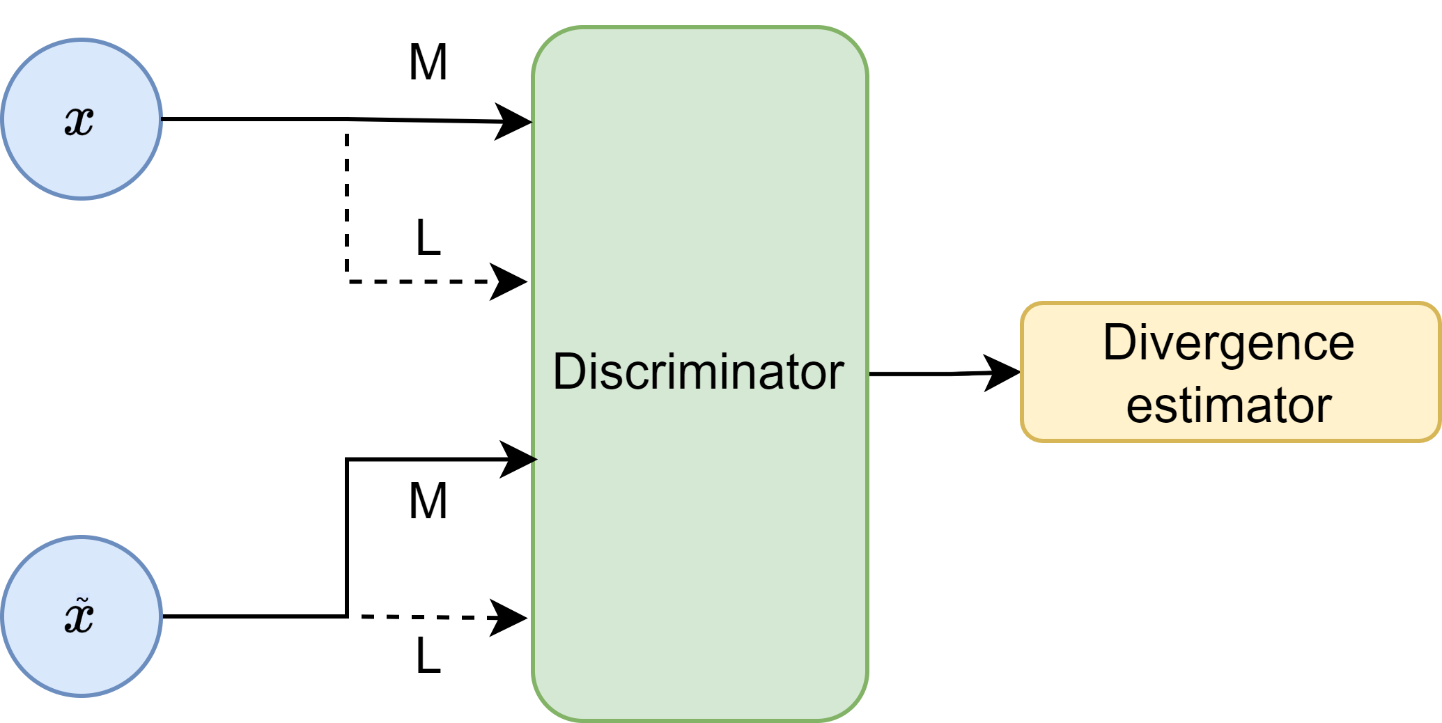
Figure 1: Architecture of the neural network-based divergence estimator to assess the dissimilarity between samples from two datasets. The discriminator takes two sets of samples as input: $M$ samples from each set to train and $L$ samples from each to infer the divergence.

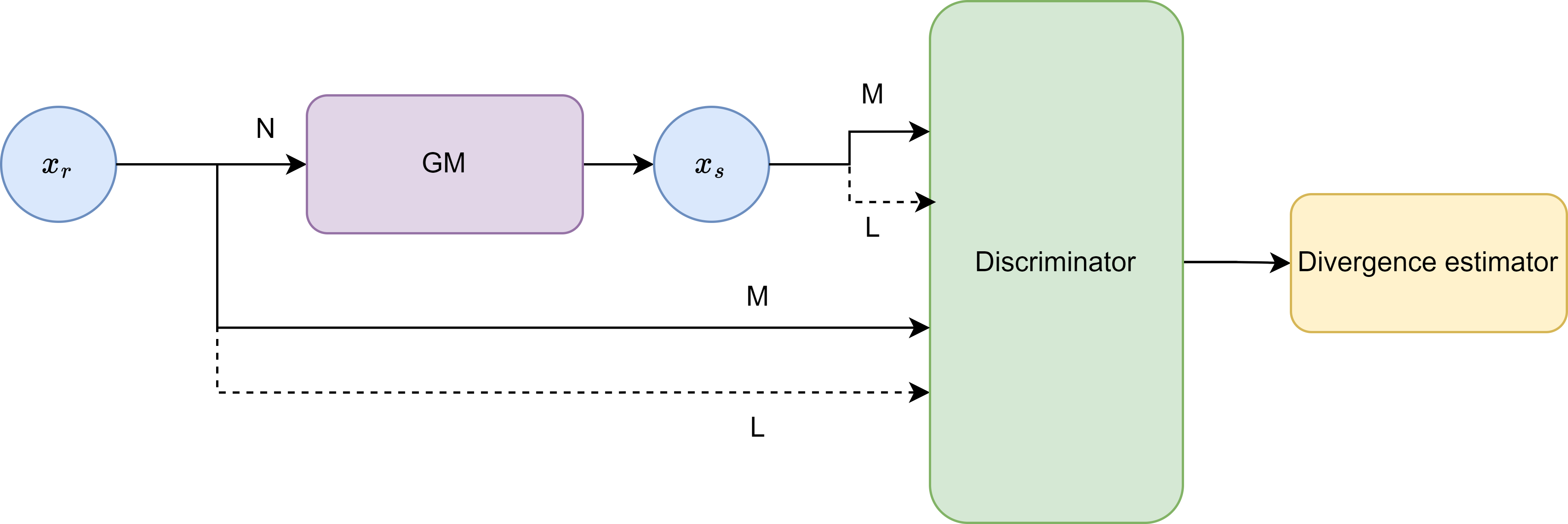
Figure 2: Generative model for divergence estimation between real and synthetic data. The generative model learns an approximation of $N$ samples from real data $x_{r}$, denoted $x_{s}$. Subsequently, $M$ samples are drawn from each distribution to train the divergence estimation discriminator. Finally, $L$ samples from each distribution are used to estimate the divergence between real and synthetic data.

This study evaluates the dissimilarity between real and synthetic data generated by a Generative Model (GM). In this context, minimizing the divergence between the real and synthetic data distributions is crucial. Ideally, the divergence should approach zero, indicating that the generated data become virtually indistinguishable from the real data. This interchangeability allows the use of synthetic data in various applications where real data might be scarce or sensitive. From the discriminator’s perspective, achieving minimal divergence implies that it cannot reliably differentiate between real and synthetic samples, indicating successful data generation. For GMs, the distributions of interest become:

• $p_{R}(x)=p(x)$, representing the real data distribution.

• $p_{S}(x)=q(x)$, representing the synthetic data distribution generated by the model.

Training data consist of $N$ samples drawn from the real data distribution, denoted $x_{r}\sim p_{R}(x)$. These data are used to train the GM, as illustrated in Fig. 2. The GM learns to approximate the real data distribution as $p_{S}(x)$, allowing us to sample from this distribution and obtain synthetic data points, $x_{s}\sim p_{S}(x)$. Following the architecture described in Fig. 1, these synthetic samples are then used along with the real data samples to train the discriminator and estimate the divergence between the real and synthetic data distributions.

4 Experiments

We aim to validate the effectiveness of our proposed divergence estimator for data generation. We achieve this through an exhaustive experimental evaluation in four different experiments, described in Table 1 designed to assess the estimator’s performance under various conditions. The initial set of experiments focuses on controlled scenarios that involve comparisons of simple theoretical data distributions. Subsequently, the complexity is gradually increased by incorporating generative scenarios that reproduce real-world applications.

Table 1: Experiments Configuration Summary. Experiments carried out to assess the effectiveness of the proposed approach. Experiments 1 and 2 investigate the impact of distribution complexity by varying the number of $M$ and $L$. Experiments 3 and 4 focus on the application to generative processes. A generative model is introduced to create synthetic data based on $N$ samples, enabling a comparison between real and synthetic scenarios.

Experiment	Compared Distributions	Generative Model	N	M	L
Experiment 1	Multivariate Gaussian Distributions	-	-	[20, 200, 2000]	[20, 200, 2000]
Experiment 2	Gaussian Mixture Distributions	-	-	[20, 200, 2000]	[20, 200, 2000]
Experiment 3	Gaussian Mixture and Synthetic Data	Gaussian Mixture Model	[10, 20, 30, … , 150]	2,000	2,000
Experiment 4	Real and Synthetic Data	CTGAN[12], VAE[23]	10,000	7,500	1,000

We comprehensively analyze the influence of sample size on the estimator’s performance. This analysis covers the impact of the size of the training and validation set for the discriminator network and the number of samples used during the generative process. To gain a deeper understanding, we evaluated different configurations for each parameter, as the table shows. For every experiment, all possible combinations of $N$, $M$, and $L$ are executed 5 times with unique random seeds. This rigorous approach employing multiple random seeds mitigates the effects of inherent randomness within training processes. Consequently, it provides a statistically robust evaluation, providing a more reliable representation of the observed trends. Ultimately, this comprehensive analysis facilitates identifying the configuration that yields the most accurate assessment of the divergence between data distributions.

The inherent variability in data nature and complexity across different experiments needs diverse divergence estimation methods. Table 2 details the specific techniques employed for each experiment, allowing for a comparative analysis whenever possible. The experiment’s level of complexity guides the selection of the validation technique.

• Analytical Divergence: This method, calculated only for $D_{\mathbb{KL}}$ for simplicity, represents the true divergence value due to the specific distributions used in the experiment.

• MC Estimated Divergence: This is a widely used estimation approach, but it can be computationally expensive.

• Discriminator Estimated Divergence: This method uses our proposed discriminator network to learn the density ratio between the two distributions and estimate the divergence.

Table 2: Experiments Configuration Summary. Validation procedure for each experiment depending on their level of complexity.

Experiment	Validation Technique
Experiment 1	Analytical, MC and Discriminator Estimations
Experiment 2	MC and Discriminator Estimations
Experiment 3	MC and Discriminator Estimations
Experiment 4	Discriminator Estimation

For complete transparency and reproducibility, the data and code used in this study are publicly available on our repository.

4.1 Experiment 1

Table 4.1 presents the results obtained for $D_{\mathbb{KL}}$ and $D_{\mathbb{JS}}$ between random multivariate Gaussian distributions. A significant advantage of this study is the availability of a closed-form solution for the KL divergence, which serves as the ground truth value. For the JS divergence, we use the MC simulation estimate as the ground truth. To ensure the reliability of this experiment, we opted for multivariate Gaussian distributions with a dimensionality of 10. This allows us to compute the true divergence values and assess the accuracy of estimating the ratio of the proposed discriminator. The results reveal a critical relationship between sample size and estimation accuracy, particularly for the discriminator-based approach. When the number of samples is limited ($M=20$, $L=20,200$), the estimated divergence from the discriminator deviates significantly from both the analytical value and the MC estimate. This suggests a potential overfitting due to insufficient data, leading to an underestimation of the true divergence. However, as the number of samples increases, the estimated divergence from the discriminator network progressively converges towards the ground truth value, followed by improved confidence interval precision. Figs. 3 and 4 confirm this trend. Both figures illustrate how increasing the number of training samples $M$ and validation samples $L$ reduces the error associated with the estimated divergence ratio. Further support for the correlation between sample size and estimation accuracy comes from the discriminator loss curves depicted in Fig. 5. As detailed in [21], the loss function converges to a constant value approximating the Jensen-Shannon divergence. The figure visually confirms this concept, as the loss curves flatten with increasing training $M$ and validation $L$ samples. In contrast, a low number of samples (e.g. $M=20$, $L=20$) results in larger fluctuations in the loss function, potentially indicating discriminator overfitting. These validations demonstrate the effectiveness of our proposed method: with sufficient training data, the discriminator can accurately learn the density ratio and provide reliable estimates of the divergences, particularly for the JS divergence.

Table 3: Impact of Training and Validating Samples on $D_{\mathbb{KL}}$ and $D_{\mathbb{JS}}$ Estimation for Experiment 1. Analytical $D_{\mathbb{KL}}$ along with MC $D_{\mathbb{KL}}$ and $D_{\mathbb{JS}}$ estimations, as well as proposed discriminator estimations for both divergences. Results are displayed for various combinations of training samples $M$ and validation samples $L$. There is a clear correlation between the number of samples used and the estimation error.

M	L	Analytical $D_{\mathbb{KL}}$	MC Estimated $D_{\mathbb{KL}}$	Discriminator Estimated $D_{\mathbb{KL}}$	MC Estimated $D_{\mathbb{JS}}$	Discriminator Estimated $D_{\mathbb{JS}}$
20	20	1.035	$1.168\pm 0.203$	$0.802\pm 0.152$	$0.320\pm 0.105$	$0.213\pm 0.072$
	200		$1.026\pm 0.221$	$0.709\pm 0.248$	$0.301\pm 0.055$	$0.200\pm 0.038$
	2000		$1.024\pm 0.193$	$0.665\pm 0.084$	$0.288\pm 0.047$	$0.209\pm 0.028$
3-3 200	20		$1.221\pm 0.422$	$0.991\pm 0.520$	$0.320\pm 0.055$	$0.289\pm 0.053$
	200		$1.114\pm 0.257$	$1.099\pm 0.227$	$0.313\pm 0.055$	$0.294\pm 0.049$
	2000		$1.026\pm 0.191$	$0.955\pm 0.101$	$0.289\pm 0.038$	$0.267\pm 0.038$
3-3 2000	20		$0.841\pm 0.190$	$0.833\pm 0.229$	$0.219\pm 0.113$	$0.218\pm 0.111$
	200		$1.004\pm 0.190$	$0.978\pm 0.185$	$0.300\pm 0.047$	$0.290\pm 0.049$
	2000		$1.055\pm 0.212$	$1.060\pm 0.200$	$0.299\pm 0.051$	$0.293\pm 0.050$

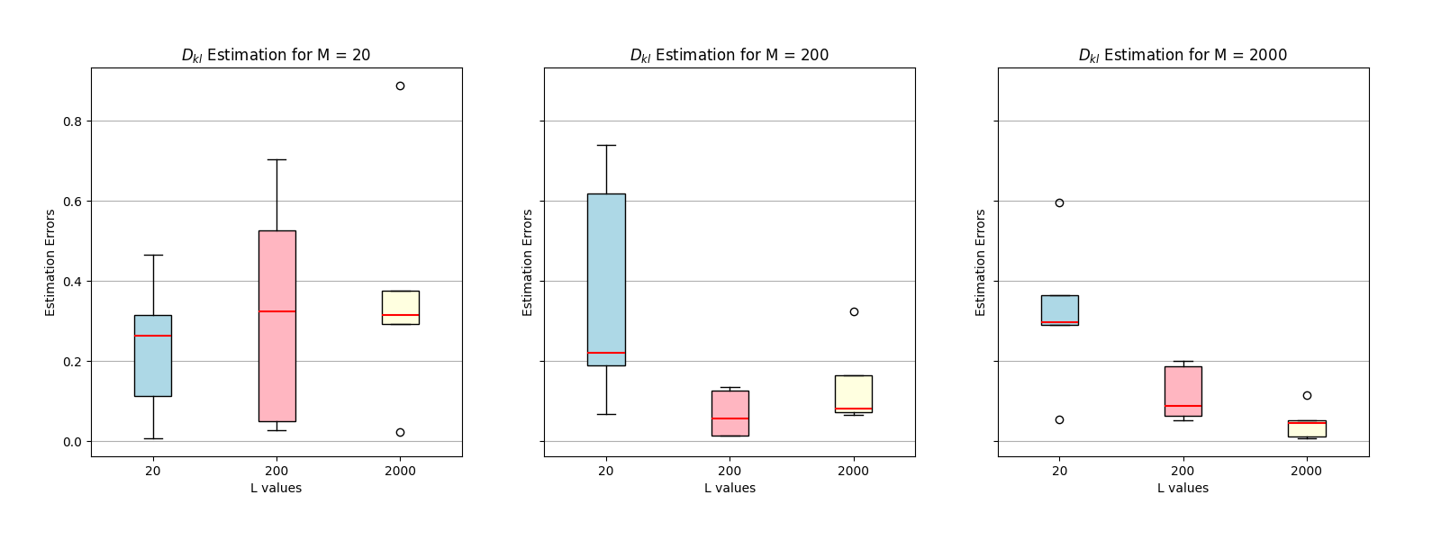
Figure 3: Estimation error representation for $D_{\mathbb{KL}}$. Results are shown for different combinations of training sample sizes $M$ and validation sample sizes $L$. As expected, a decrease and precision in the error is observed with increasing values of $M$ and $L$.

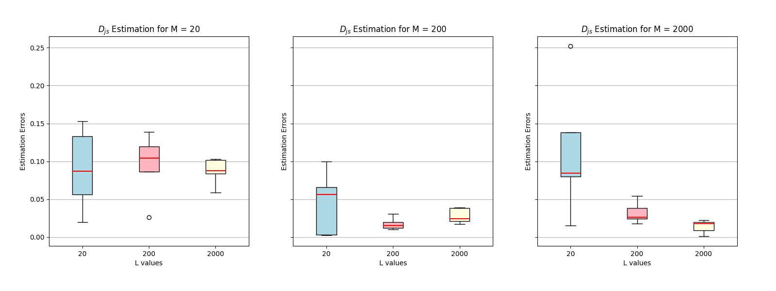
Figure 4: Estimation error representation for $D_{\mathbb{JS}}$. Results are shown for different combinations of training sample sizes $M$ and validation sample sizes $L$. As expected, a decrease and precision in the error is observed with increasing values of $M$ and $L$.

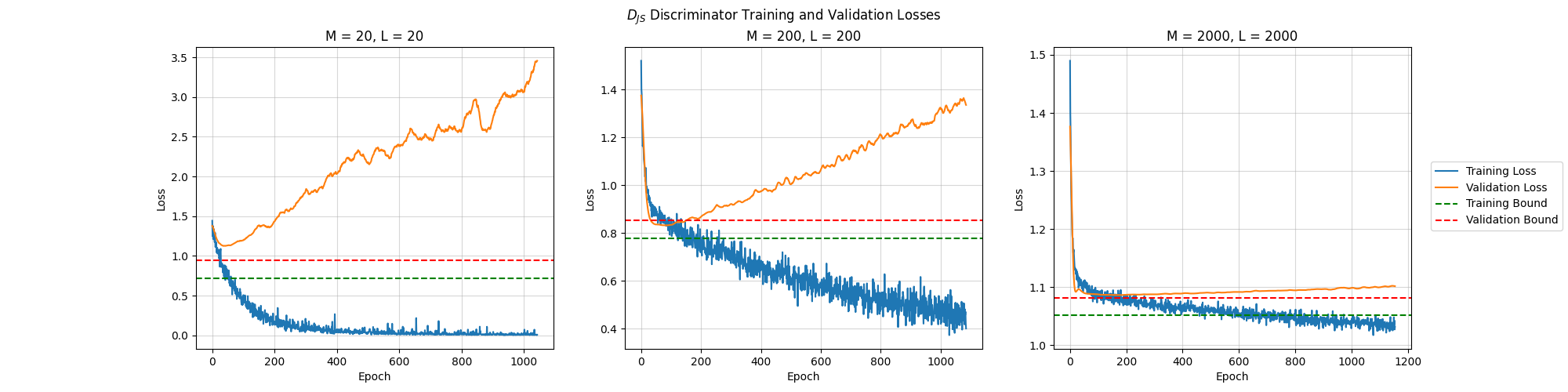
Figure 5: Discriminator loss curves for Experiment 1. The loss curves show a clear overfitting due to low sample sizes. Green and red dashed lines represent theoretical convergence values.

Leveraging Experiment 1, we further emphasize the superior robustness of our proposed approach in estimating the JS divergence, regardless of variations in distribution separation. Fig. 6 illustrates the relation between estimated divergences and ground truth values as the separation between two 4-dimensional multivariate Gaussian distributions increases. As observed, the relation for the JS divergence remains almost linear until it approaches 1. While the relationship appears less linear for values near 1, it is important to note that the primary application of this discriminator lies in comparing similar distributions. Therefore, the focus should be placed on the performance for low JS divergences. Meanwhile, the KL divergence exhibits a nonlinear relation starting from the first comparisons, with the estimated KL deviating from the ground truth probably because of bias introduced by the discriminator.

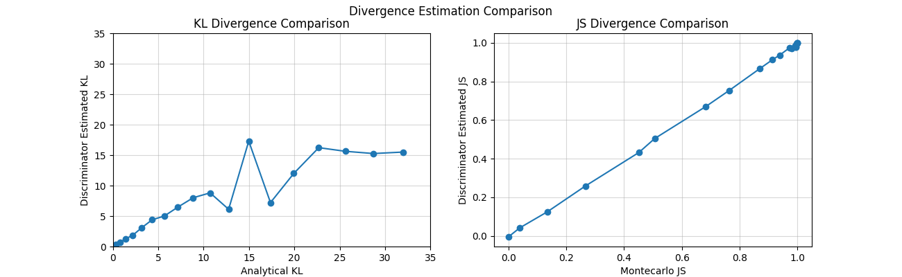
Figure 6: Relation between ground truth and estimated divergences as distribution separation increases.

4.2 Experiment 2

This experiment investigates the performance of the proposed divergence estimation method in Gaussian mixture distributions. These distributions offer a higher level of complexity compared to those used in Experiment 1. Each Gaussian mixture distribution comprises two independent isotropic Gaussian components with distinct mixing probabilities (weights assigned to each component within the mixture). Unlike the prior case, where analytical ground truth for divergence was obtainable, here and in the following experiment, we rely solely on MC approximations as ground truth. Similar results were obtained for this experiment compared to the first. Tables 4 and 5 focus on a practical range for training sample sizes $M$ and validation sample sizes $L$ (both set to $200,2000$) and present the estimated divergences obtained using our proposed method compared to MC estimates. The results demonstrate that, for both divergences, the proposed method achieves results comparable to the MC estimates. These findings further support the previously observed correlation between sample size and estimation accuracy. Additionally, for both divergence measures, we observe a narrowing of confidence intervals with increasing sample sizes. This trend indicates that the estimation becomes progressively more precise as the amount of available data increases. Overall, the results from this experiment underscore the effectiveness of the proposed method in estimating divergences for more intricate distributions, such as Gaussian mixtures. The remaining analysis can be found in the Appendix.

Table 4: Impact of Training and Validating Samples on $D_{\mathbb{KL}}$ Estimation for Experiment 2. MC and proposed method $D_{\mathbb{KL}}$ estimation for various combinations of training and validation samples $M$ and $L$. The results highlight a clear correlation between the number of samples used and the estimation error.

M	L	MC Estimated $D_{\mathbb{KL}}$	Discriminator Estimated $D_{\mathbb{KL}}$
200	200	$2.669\pm 0.118$	$2.686\pm 0.294$
	2000	$2.887\pm 0.045$	$3.037\pm 0.517$
2000	200	$2.710\pm 0.100$	$2.628\pm 0.357$
	2000	$2.850\pm 0.071$	$2.913\pm 0.129$

Table 5: Impact of Training and Validating Samples on $D_{\mathbb{JS}}$ Estimation for Experiment 2. MC and proposed method $D_{\mathbb{JS}}$ estimation for various combinations of training and validation samples $M$ and $L$. The results highlight a clear correlation between the number of samples used and the estimation error.

M	L	MC Estimated $D_{\mathbb{JS}}$	Discriminator Estimated $D_{\mathbb{JS}}$
200	200	$0.392\pm 0.013$	$0.374\pm 0.020$
	2000	$0.428\pm 0.009$	$0.412\pm 0.009$
2000	200	$0.415\pm 0.020$	$0.412\pm 0.019$
	2000	$0.423\pm 0.014$	$0.420\pm 0.013$

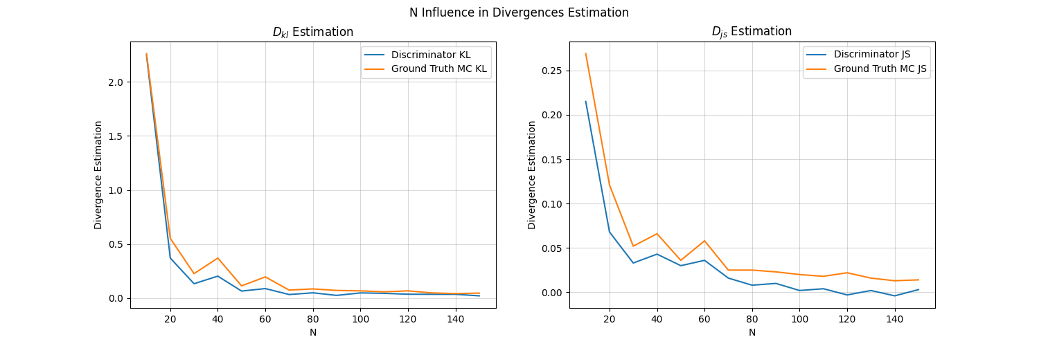
Figure 7: Estimated $D_{\mathbb{KL}}$ and $D_{\mathbb{JS}}$ compared to ground truth values for varying sample sizes of $N$. Note the independent y-axes for each divergence measure due to their inherent scale differences, with $D_{\mathbb{JS}}$ exhibiting lower values than $D_{\mathbb{KL}}$.

4.3 Experiment 3

The following experiments introduce the concept of a generative process, where synthetic data are generated based on $N$ samples from a certain data distribution. We investigate the influence of the quality of the GM in terms of the number of samples used to generate. This specific experiment uses a Gaussian mixture with two components as the real distribution. We employ a Gaussian mixture model (GMM) as the GM. The trained GMM then generates synthetic data that serve as an approximation of the real data. Finally, we estimate the divergence using our approach with a sufficient number of samples to achieve a low confidence interval and compare it to the MC simulation estimation. We analyze the behavior of the GMM under different training configurations, varying the number of training samples $N$. Since previous experiments demonstrated that a high number of samples for both $M$ and $L$ achieve better divergence estimations, for this experiment we have fixed $M=2000$ and $L=2000$. We compare the estimated divergence errors for this combination of training samples $M$ and validation $L$ used by the divergence estimator. Fig. 7 shows the estimated divergences as $N$ increases. The results demonstrate a clear correlation between the size of the training data for the GMM, $N$, and the estimated divergence errors. When the GMM is poorly trained due to a limited number of samples ($N=10$), it is unable to effectively capture the underlying data patterns. This leads to generated data that significantly deviate from the real distribution. Consequently, the real divergence values increase significantly and a large estimation error occurs, particularly for unbounded $D_{\mathbb{KL}}$. $D_{\mathbb{JS}}$, which is inherently bounded between 0 and 1, exhibits less extreme error values. As the number of training samples for the GMM increases ($N=200$ and $N=2000$), the generated data become more representative of the real distribution. This results in lower divergence values and reduced estimation errors for $D_{\mathbb{KL}}$ and $D_{\mathbb{JS}}$. This finding supports the validity of our proposed validation technique for generative processes involving Gaussian mixture distributions.

4.4 Experiment 4

The final experiment introduces a more realistic setting by incorporating a real-world dataset along with its synthetic counterpart generated using a GM. This scenario retains the concept of a generative process, but the target distribution becomes the real-world data itself. The dataset chosen is Adult. As described in [24], it contains information on $32,561$ individuals used to predict their annual income exceeding $50,000. It represents an extract from the $1994$ U.S. Census database [25]. For our experiments and after the previous analysis done, we used a subset of $10,000$ samples obtained from [26]. This dataset comprises 14 features encompassing various data types, including categorical, binary, and integer values. Based on the previous analysis of the influence of the sample size, we fixed the hyperparameters for this experiment at $N=10000$, $M=7500$, and $L=1000$. To evaluate GMs, we compared the performance of two state-of-the-art approaches: the widely used CTGAN[12] and the VAE-based generator proposed in [23] (VAE), which achieved superior results based on several validation criteria. Table 6 confirms this, obtaining lower divergence results for [23]. This experiment focuses on evaluating the ability of the divergence estimator to assess the similarity between the real data and its synthetic counterpart. This experiment provides valuable insights into the practical application of the proposed method in real-world scenarios where measuring the similarity between real and synthetic data is crucial.

Table 6: Comparison of Generative Models for Real-World Data. Similarity comparison between real data and their synthetic counterparts generated by each model using estimated divergences, $D_{\mathbb{KL}}$ and $D_{\mathbb{JS}}$. Lower values in both metrics indicate a greater similarity between real and synthetic data.

CTGAN $D_{\mathbb{KL}}$	VAE $D_{\mathbb{KL}}$	CTGAN $D_{\mathbb{JS}}$	VAE $D_{\mathbb{JS}}$
$0.342\pm 0.016$	$0.185\pm 0.030$	$0.138\pm 0.002$	$0.099\pm 0.002$

5 Conclusion

This research proposes a novel and effective approach for validating synthetic tabular data generated by various models. The core of this method lies in using a divergence estimator based on a probabilistic classifier to capture the discrepancies between the real and synthetic data distributions. This approach overcomes the limitations associated with traditional marginal divergence comparisons by considering the joint distribution. While marginal comparisons assess the similarity of individual features between real and synthetic data, they can be misleading. Even if the marginal distributions of each feature appear similar, the joint distribution, which captures the relationships between features, may differ significantly. This can lead to unrealistic synthetic data, where individual features appear plausible but their co-occurrences are not representative of the real data. By considering the joint distribution, our proposed method provides a more comprehensive assessment of the quality of synthetic tabular data.

The efficacy of the proposed method is comprehensively evaluated through a series of experiments with progressively increasing complexity. The initial phase establishes a solid foundation by analyzing the performance in controlled scenarios with well-defined theoretical distributions. The results demonstrate that the accuracy of divergence estimates is highly dependent on the amount of training data available for both the GM and the divergence estimator network. Subsequent experiments explore more intricate scenarios involving Gaussian mixture distributions and real-world datasets. The findings consistently support the effectiveness of the proposed method in approximating the true divergences. Our emphasis in this paper has been to show the advantages of using divergences as synthetic data validation for tabular data.

This research offers significant contributions that extend beyond the specific tabular data validation domain. The proposed methodology facilitates better validation practices for various fields dependent on GMs. Its key strength lies in the capture of complex relationships between different data distributions, leading to more robust and reliable validation processes. In addition to the positive results, the study also highlights the importance of the quality of the GM. When it is inadequately trained due to insufficient data, it can significantly impact the accuracy of the divergence estimation. This emphasizes the need to carefully consider GM training procedures to ensure reliable validation results.

Several promising avenues exist for future research. One direction involves exploring the potential to extend the proposed approach to more complex data structures, such as images or time series data. Additionally, investigating the integration of this validation technique within GM training pipelines could enable the development of self-improving GMs that can automatically adjust their parameters to generate data that closely resemble the target distribution. Finally, developing a robust methodology to estimate divergences when limited samples are available presents a crucial challenge. Addressing this challenge would further enhance the versatility and practicality of the proposed validation technique in real-world scenarios with restricted data availability. Furthermore, it would be beneficial to investigate alternative density ratio estimation techniques, such as those presented in [27, 28]. These methods may offer advantages in terms of sample size requirements, estimation error, or other relevant properties.

Acknowledgments

This research was supported by GenoMed4All and SYNTHEMA projects. Both have received funding from the European Union’s Horizon 2020 research and innovation program under grant agreement No 101017549 and 101095530, respectively. The authors declare that they have no known competing financial interests or personal relationships that could have appeared to influence the work reported in this paper.

Appendix

Table 7: Impact of Training and Validating Samples on $D_{\mathbb{KL}}$ and $D_{\mathbb{JS}}$ Estimation for Experiment 2. Analytical $D_{\mathbb{KL}}$ along with MC $D_{\mathbb{KL}}$ and $D_{\mathbb{JS}}$ estimations, as well as proposed discriminator estimations for both divergences. Results are displayed for various combinations of training samples $M$ and validation samples $L$. There is a clear correlation between the number of samples used and the estimation error.

M	L	MC Estimated $D_{\mathbb{KL}}$	Discriminator Estimated $D_{\mathbb{KL}}$	MC Estimated $D_{\mathbb{JS}}$	Discriminator Estimated $D_{\mathbb{JS}}$
20	20	$3.245\pm 0.820$	$1.832\pm 0.912$	$0.490\pm 0.083$	$0.371\pm 0.078$
	200	$2.699\pm 0.095$	$1.193\pm 0.430$	$0.439\pm 0.017$	$0.328\pm 0.058$
	2000	$2.833\pm 0.032$	$1.512\pm 0.381$	$0.423\pm 0.006$	$0.331\pm 0.039$
200	20	$2.639\pm 0.404$	$3.101\pm 0.779$	$0.405\pm 0.066$	$0.340\pm 0.114$
	200	$2.669\pm 0.118$	$2.686\pm 0.294$	$0.392\pm 0.013$	$0.374\pm 0.020$
	2000	$2.887\pm 0.045$	$3.037\pm 0.517$	$2.887\pm 0.045$	$3.037\pm 0.517$
2000	20	$2.974\pm 0.626$	$2.771\pm 0.751$	$0.481\pm 0.090$	$0.474\pm 0.096$
	200	$2.710\pm 0.100$	$2.628\pm 0.357$	$0.415\pm 0.020$	$0.412\pm 0.019$
	2000	$2.850\pm 0.071$	$2.913\pm 0.129$	$0.423\pm 0.014$	$0.420\pm 0.013$

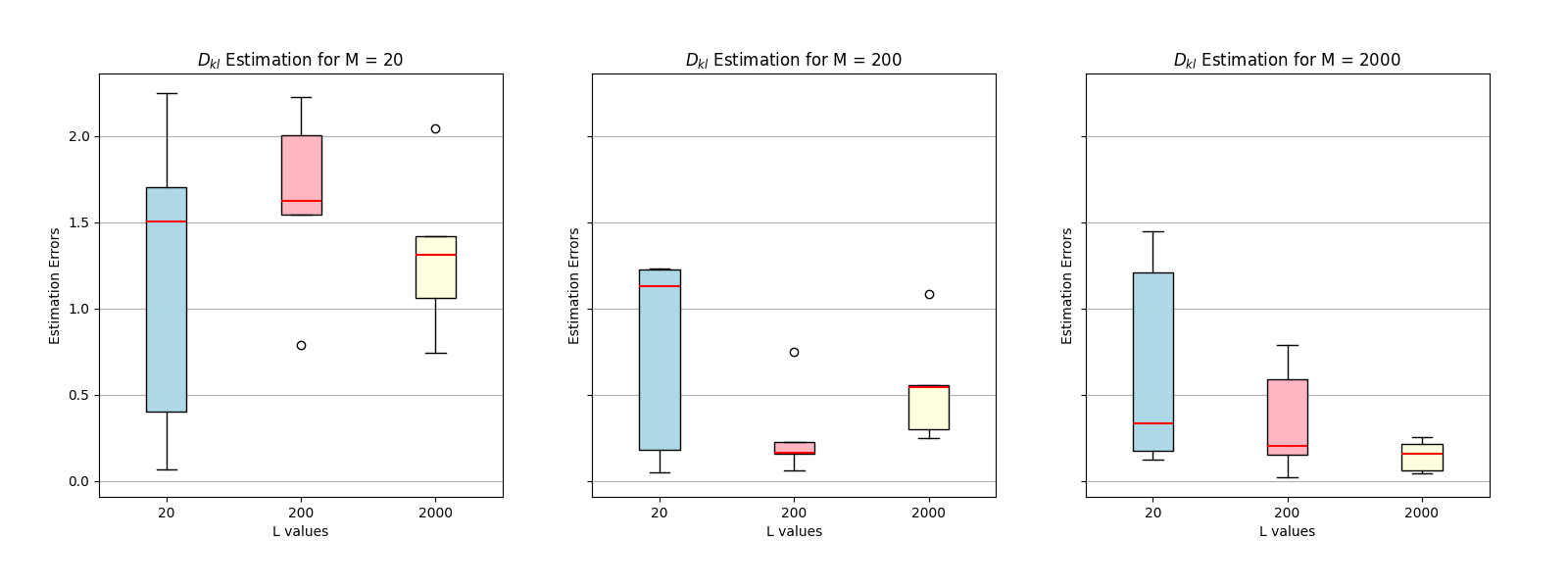
Figure 8: Estimation error representation for $D_{\mathbb{KL}}$. Results are shown for different combinations of training sample sizes $M$ and validation sample sizes $L$. As expected, a decrease and precision in the error is observed with increasing values of $M$ and $L$.

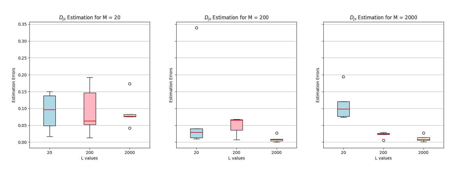
Figure 9: Estimation error representation for $D_{\mathbb{JS}}$. Results are shown for different combinations of training sample sizes $M$ and validation sample sizes $L$. As expected, a decrease and precision in the error is observed with increasing values of $M$ and $L$.

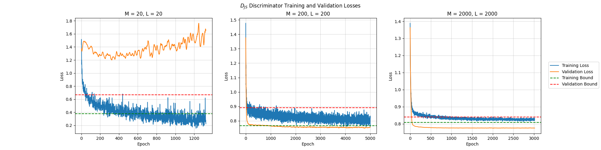
Figure 10: Discriminator loss curves for Use Case 1. The loss curves show a clear overfitting due to low sample sizes. Green and red dashed lines represent theoretical convergence values.

Building on Experiment 1, Experiment 2 uses the same validation process. Table 7 expands on previous findings by presenting the performance of our approach with a limited number of training and validation samples for the divergence estimator. The results demonstrate convergence towards the ground truth divergence values as the number of samples used for both training and validation increases. This trend is further corroborated by Figs. 8 and 9. Additionally, Fig. 10 explores the behavior of the discriminator’s loss function for various combinations of sample sizes.

References

- [1] Aryan Jadon and Shashank Kumar. Leveraging generative ai models for synthetic data generation in healthcare: Balancing research and privacy. 2023 International Conference on Smart Applications, Communications and Networking (SmartNets), pages 1–4, 2023.
- [2] Handenur Caliskan, Omer Faruk Yayla, and Yakup Genç. A comparative analysis of synthetic data generation with vae and ctgan models on financial credit loan offer data. 2023 8th International Conference on Computer Science and Engineering (UBMK), pages 212–217, 2023.
- [3] Deepak Talwar, Sachin Guruswamy, Naveen Ravipati, and Magdalini Eirinaki. Evaluating validity of synthetic data in perception tasks for autonomous vehicles. pages 73–80, 08 2020.
- [4] Tim Salimans, Ian Goodfellow, Wojciech Zaremba, Vicki Cheung, Alec Radford, and Xi Chen. Improved techniques for training gans, 2016.
- [5] Martin Heusel, Hubert Ramsauer, Thomas Unterthiner, Bernhard Nessler, and Sepp Hochreiter. Gans trained by a two time-scale update rule converge to a local nash equilibrium, 2018.
- [6] Tianyi Zhang, Varsha Kishore, Felix Wu, Kilian Q. Weinberger, and Yoav Artzi. Bertscore: Evaluating text generation with bert, 2020.
- [7] Kishore Papineni, Salim Roukos, Todd Ward, and Wei-Jing Zhu. Bleu: a method for automatic evaluation of machine translation. In Proceedings of the 40th Annual Meeting on Association for Computational Linguistics, ACL ’02, page 311–318, USA, 2002. Association for Computational Linguistics.
- [8] Zhengping Che, Yu Cheng, Shuangfei Zhai, Zhaonan Sun, and Yan Liu. Boosting deep learning risk prediction with generative adversarial networks for electronic health records, 2017.
- [9] Fan Yang, Zhongping Yu, Yunfan Liang, Xiaolu Gan, Kaibiao Lin, Quan Zou, and Yifeng Zeng. Grouped correlational generative adversarial networks for discrete electronic health records. In 2019 IEEE International Conference on Bioinformatics and Biomedicine (BIBM), pages 906–913, 2019.
- [10] Sina Rashidian, Fusheng Wang, Richard Moffitt, Victor Garcia, Anurag Dutt, Wei Chang, Vishwam Pandya, Janos Hajagos, Mary Saltz, and Joel Saltz. Smooth-gan: Towards sharp and smooth synthetic ehr data generation. In Martin Michalowski and Robert Moskovitch, editors, Artificial Intelligence in Medicine, pages 37–48, Cham, 2020. Springer International Publishing.
- [11] André Gonçalves, Priyadip Ray, Braden Soper, Jennifer Stevens, Linda Coyle, and Ana Sales. Generation and evaluation of synthetic patient data. BMC Medical Research Methodology, 20, 05 2020.
- [12] Lei Xu, Maria Skoularidou, Alfredo Cuesta-Infante, and Kalyan Veeramachaneni. Modeling tabular data using conditional gan, 2019.
- [13] Saloni Dash, Andrew Yale, Isabelle Guyon, and Kristin P. Bennett. Medical time-series data generation using generative adversarial networks. In Martin Michalowski and Robert Moskovitch, editors, Artificial Intelligence in Medicine, pages 382–391, Cham, 2020. Springer International Publishing.
- [14] Joshua Snoke, Gillian Raab, Beata Nowok, Chris Dibben, and Aleksandra Slavkovic. General and specific utility measures for synthetic data, 2017.
- [15] Mikel Hernandez, Gorka Epelde, Ane Alberdi, Rodrigo Cilla, and Debbie Rankin. Synthetic tabular data evaluation in the health domain covering resemblance, utility, and privacy dimensions. Methods of information in medicine, 62, 01 2023.
- [16] Aoting Hu, Renjie Xie, Zhigang Lu, Aiqun Hu, and Minhui Xue. Tablegan-mca: Evaluating membership collisions of gan-synthesized tabular data releasing, 2021.
- [17] Shuo Wang, Carsten Rudolph, Surya Nepal, Marthie Grobler, and Shangyu Chen. Part-gan: Privacy-preserving time-series sharing. In Igor Farkaš, Paolo Masulli, and Stefan Wermter, editors, Artificial Neural Networks and Machine Learning – ICANN 2020, pages 578–593, Cham, 2020. Springer International Publishing.
- [18] Zilong Zhao, Aditya Kunar, Hiek Van der Scheer, Robert Birke, and Lydia Y. Chen. Ctab-gan: Effective table data synthesizing, 2021.
- [19] Allan Tucker, Zhenchen Wang, Ylenia Rotalinti, and Puja Myles. Generating high-fidelity synthetic patient data for assessing machine learning healthcare software. NPJ digital medicine, 3(1):1–13, 2020.
- [20] Charlie Frogner and Tomaso Poggio. Fast and flexible inference of joint distributions from their marginals. In Kamalika Chaudhuri and Ruslan Salakhutdinov, editors, Proceedings of the 36th International Conference on Machine Learning, volume 97 of Proceedings of Machine Learning Research, pages 2002–2011. PMLR, 09–15 Jun 2019.
- [21] Louis C Tiao. Density Ratio Estimation for KL Divergence Minimization between Implicit Distributions. tiao.io, 2018.
- [22] Eduard Čech and M. Katětov. Point Sets. Academia, Publishing House of the Czechoslovak Academy of Sciences, 1969.
- [23] Patricia A Apellániz, Juan Parras, and Santiago Zazo. An improved tabular data generator with vae-gmm integration. arXiv preprint arXiv:2404.08434, 2024.
- [24] Barry Becker and Ronny Kohavi. Adult. UCI Machine Learning Repository, 1996. DOI: https://doi.org/10.24432/C5XW20.
- [25] Ron Kohavi. Census Income. UCI Machine Learning Repository, 1996. DOI: https://doi.org/10.24432/C5GP7S.
- [26] Neha Patki, Roy Wedge, and Kalyan Veeramachaneni. The synthetic data vault. In IEEE International Conference on Data Science and Advanced Analytics (DSAA), pages 399–410, Oct 2016.
- [27] Kristy Choi, Chenlin Meng, Yang Song, and Stefano Ermon. Density ratio estimation via infinitesimal classification. In Gustau Camps-Valls, Francisco J. R. Ruiz, and Isabel Valera, editors, Proceedings of The 25th International Conference on Artificial Intelligence and Statistics, volume 151 of Proceedings of Machine Learning Research, pages 2552–2573. PMLR, 28–30 Mar 2022.
- [28] Benjamin Rhodes, Kai Xu, and Michael U. Gutmann. Telescoping density-ratio estimation, 2020.