An Efficient Compression Method for Sign Information of
DCT Coefficients via Sign Retrieval
Abstract
Compression of the sign information of discrete cosine transform coefficients is an intractable problem in image compression schemes due to the equiprobable occurrence of the sign bits. To overcome this difficulty, we propose an efficient compression method for such sign information based on phase retrieval, which is a classical signal restoration problem attempting to find the phase information of discrete Fourier transform coefficients from their magnitudes. In our compression strategy, the sign bits of all the AC components in the cosine domain are excluded from a bitstream at the encoder and are complemented at the decoder by solving a sign recovery problem, which we call sign retrieval. The experimental results demonstrate that the proposed method outperforms previous techniques for sign compression in terms of a rate-distortion criterion. Our method implemented in Python language is available from https://github.com/ctsutake/sr.
Keywords. Image coding, discrete cosine transform, sign information, phase retrieval, sign retrieval, compressive sampling, convex optimization.
1 Introduction
The discrete cosine transformation (DCT) [1] is known as an essential building block for image compression technology that can approximately represent a natural image by using a reduced number of coefficients in the cosine domain [2]. Actual image compression methods, e.g., JPEG, first divide an original image into blocks and then apply the DCT to the blocks followed by a quantization process. Entropy coding is finally performed for efficient binary representations of the quantization indices, in which we face a compression problem for the sign information due to the equiprobable occurrence of the sign bits [3]. We address this sign compression problem for DCT coefficients in this paper.
We briefly summarize seminal works developed to tackle this challenging problem. Tu and Tran [4] proposed a technique inspired by sub-band coding in which DCT coefficients of specific frequency bands are collected in new blocks, and the sign bits are then compressed efficiently by exploiting their correlation in a new block, as was done in EBCOT [5]. Ponomarenko et al. [6] proposed a two-stage technique, where the pixel values of a target block are first estimated from those of already encoded and decoded neighbor blocks and then used to predict the sign bits of DCT coefficients. Since there is a possibility that several predicted sign bits will be incorrect, they proposed transmitting the residual information, i.e., the prediction error, comprising compressible binaries. Clare et al. [7] proposed a compression technique known as sign data hiding in which the encoding of one sign bit for each sub-block can be avoided under a mild condition. There are many other works in addition to those mentioned above, e.g., [8, 9, 10].
To achieve more efficient compression of the sign bits, we propose a novel method based on an approach significantly different from the current literature. Our method relies on a classical signal processing method, referred to as phase retrieval (PR) [11] detailed in Section 2. Specifically, we first retrieve the sign information of all the AC components in the cosine domain only from their magnitudes, and the encoder and decoder then respectively compose and parse a tailored bitstream that includes the residual information to compensate for errors in the retrieved signs, as was done in [6]. To the best of our knowledge, this is the first paper that incorporates the PR methodology into image compression. We show through experiments that our method outperforms the previous ones in terms of a rate-distortion criterion.
1.1 Contributions
The main contributions of this paper are threefold:
-
•
A mathematical formulation of a non-convex retrieval problem for the sign information in DCT-based image compression, which we call sign retrieval (SR).
- •
-
•
Construction of an efficient convex solution method that combines a classical Fienup algorithm [14] with a cascading technique.
Note that Salehi et al. [15] proposed a CS-based convex phase retrieval technique similar to our method. They used a set of Gaussian measurements [16] to guarantee a theoretical performance, but block-wise cosine measurements were not considered. Our study is thus located on a different position from the measurement viewpoint.
1.2 Paper Organization
The rest of this paper is organized as follows. In Section 2, we summarize a classical PR problem [11] and its solution [12]. Section 3 elaborates the proposed method. In Section 4, we report the experimental results and discuss the advantages of our method. We conclude in Section 5 with a brief summary and mention of future work.
1.3 Notations
Throughout this paper, we denote a 2D image and its pixels by and , respectively, where and are horizontal and vertical indices, respectively. Let and be a block of the image and its pixels, respectively, where and are block indices, and and are indices in the block. Let and be the DFT and DCT coefficients of the image and the block , respectively; and are indices in the Fourier and cosine domains, respectively. We assume that image and block sizes are and , respectively. The inner product operator and the norm are denoted by and , respectively.
2 Phase Retrieval
Phase retrieval [11] is a classical signal processing method that attempts to solve a non-convex problem of the form
| (1) |
Note that (1) cannot be solved within polynomial time because of its NP-hardness [17]. To avoid this difficulty, Goldstein and Studer [12] proposed a convex relaxation of (1), referred to as PhaseMax:
| (2) |
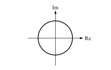
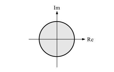
where is the so-called anchor vector. Figure 1 shows a geometrical interpretation of constraints in the Fourier domain, where (a) and (b) correspond to (1) and (2), respectively. We have to find the phase information from a non-convex circle in (1), while (2) allows the retrieval in a convex disk.
Goldstein and Studer showed the surprising result that (1) and (2) are equivalent if the number of samples is higher than the number of pixels, i.e., oversampled, and is chosen in such a way that the constant
| (3) |
is sufficiently large. In other words, the original image including the exact phase information can be recovered from a set of magnitude measurements in the Fourier domain.
3 Proposed method
3.1 Encoder and Decoder
To achieve efficient compression of the sign information, we modify a bitstream standardized in a conventional DCT-based image compression method, e.g., JPEG. We construct the following encoder and decoder, in which denotes a degraded version of the original DCT coefficient obtained by means of the quantization process in the conventional image compression method.
Encoder: The sign information of all the AC components in the cosine domain are excluded from a bitstream. In other words, only the magnitudes are first compressed by suitable entropy coding. The encoder then performs SR defined in the next subsection to retrieve the sign information. Finally, since there is a possibility that several retrieved signs will be incorrect, we append the residual information
| (4) |
to the bitstream, where is the retrieved sign and is the XOR operator.
Decoder: The decoder first parses the bitstream to obtain the magnitudes and the residues . The sign information is then retrieved via SR using only in the same way as in the encoder. Finally, the retrieved signs including errors are corrected by .
Note that the residual information hopefully has many zeros but few ones, and is thus compressible, if the sign bits are retrieved correctly to some extent. In fact, we can recover almost all the sign bits correctly, as will be shown in Section 4.
3.2 Sign Retrieval and Its Convex Relaxation
According to (1), retrieval of the sign information can be formulated as a non-convex optimization problem:
| (5) |
which we call sign retrieval in our image compression scenario. As in [18], it can be interpreted as a special case of (1) by replacing the phase information and the Fourier magnitude with the sign information and the cosine magnitude, respectively. Motivated by this, we formulate a convex relaxation of (5) based on (2) as follows:
| (6) |
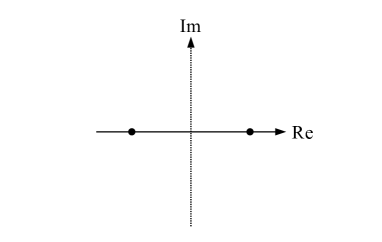
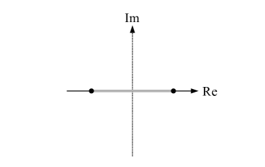
Figure 2 shows constraints of (5) and (6), similarly to Fig. 1. There are no imaginary parts in the cosine domain, so that the constraint in (6) is represented as a convex real line.
We then apply the CS theory [13] to (6) because of its ill-posedness from the sampling viewpoint: the DFT coefficients are oversampled in (2) while the number of DCT coefficients is equivalent to that of the pixels in (6). The theory claims that a sparse signal can be restored from a set of few measurements by solving a constrained -norm minimization problem. In our compression setting, can be seen as the measurements in the cosine domain, so that we introduce an norm function in (6). Let be a semi-orthonormal matrix satisfying for promoting the sparsity of the entire image . We formulate a regularized SR problem as
| (7) |
where is a regularization parameter. By solving this, note that the retrieved sign can be given as
where is a DCT coefficient of a block in .
3.3 Solution to (7)
We elaborate hereafter an actual solution method for (7). We apply the Fienup algorithm [14], a conventional but efficient solution method for the PR problem (1), to our SR. The original Fienup algorithm features two building blocks: proximal operations [19] and projection onto non-convex constraint sets (Fig. 1(a)).
With this in mind, since the constraint is convex in our problem, we first introduce the corresponding convex set
Let denote a union of all the set , and let
be an indicator function. The Fienup algorithm for (7) can be described as the following three steps by performing variable splitting [20]:
| (8) | ||||
| (9) | ||||
| (10) |
where is the number of iterations, and is a positive penalty parameter. Note that (8), (9), and (10) are proximal operations in terms of , , and , respectively. According to [19], we have the closed-form solutions of these problems as follows:
| (11) | ||||
| (12) | ||||
| (13) |
where , and is the projection operator onto . The iteration is performed until reaches the maximum count .
Finally, we discuss how to determine the anchor vector . In PR, because is chosen so that is sufficiently large, we also determine on the basis of this criterion. To this end, we first use a random initialization method, as in [12], and then solve (7) repeatedly by setting , where is the solution of the former iteration. This is because would be a better approximation of , leading to a higher . We cascade the solution times, and the entire algorithm is described as Algorithm 1.


4 Experimental Results
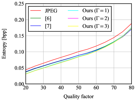
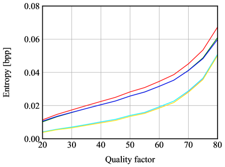
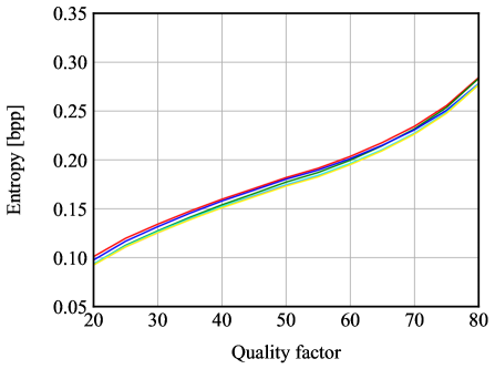
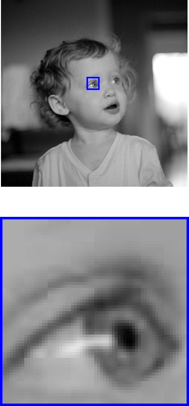
To evaluate the effectiveness of our method, we implemented it in JPEG with and compared it with [6] and [7]. We used the original images shown in Fig. 3, which were generated by cropping regions of images from the MIT-Adobe FiveK Dataset [21]. All the images were compressed with the quality factor varied from to . Because all the methods yield the same error against the original image, we evaluated the entropy [bpp] required for compressing the sign bits, e.g., in our method.
The parameters and were set to and , respectively. We ran iterations and varied the number of cascading from to because it significantly affects the accuracy of . A translation invariant version [22] of the -th order Symmlet transformation [23] was used as , leading to .
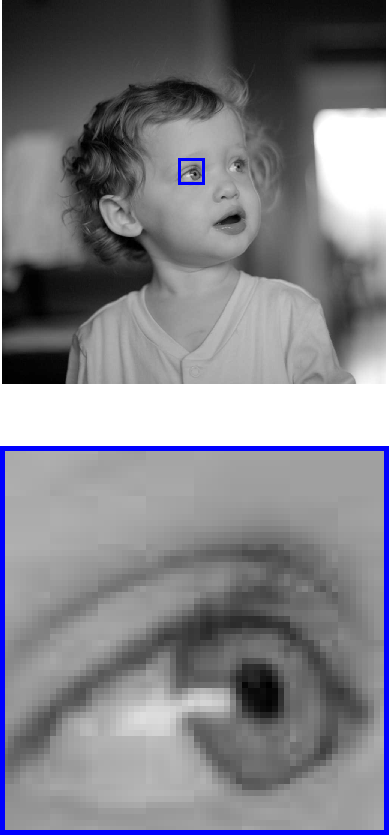
Figure 4 shows the entropy required to transmit the sign information of the DCT coefficients by each method. Compared to the previous techniques, our method with had a lower entropy. This result can be improved by increasing , which demonstrates that cascading is effective in our method. Figure 5 shows several examples of reconstructed images, where (a) is a JPEG image and (b) and (c) are reconstructed images using random sign bits and those retrieved by Algorithm 1 with , respectively. While (b) was completely degraded, (c) was very close to (a), indicating that most of the sign bits were correctly retrieved. Note that in our method, the errors in (b) and (c) were eventually corrected by using to obtain exactly the same image as (a). However, when used with Algorithm 1, the residual bits consisted of many zeros and few ones, resulting in small entropy values for the sign information, as shown in Fig. 4. These results demonstrate the advantages of the proposed method over the previous techniques from the rate-distortion point of view.
5 Conclusion
In this paper, we addressed an intractable sign compression problem for DCT coefficients in image compression by developing a method based on PR. Specifically, we first formulated a PR-based non-convex optimization problem, i.e., SR, and its convex relaxation by means of the -norm regularization. The resulting optimization problem was solved by the cascaded Fienup algorithm. Our method was validated by a comparison with previous techniques. We presume our method can be applied to any DCT-based compression standard, such as HEVC [24] or VVC [25], which we will verify in future work.
References
- [1] N. Ahmed, T. Natarajan, and K. R. Rao, “Discrete cosine transform,” IEEE Transactions on Computers, vol. C-23, no. 1, pp. 90–93, 1974.
- [2] W.-H. Chen and W. Pratt, “Scene adaptive coder,” IEEE Transactions on Communications, vol. 32, no. 3, pp. 225–232, 1984.
- [3] E. Y. Lam and J. W. Goodman, “A mathematical analysis of the DCT coefficient distributions for images,” IEEE Transactions on Image Processing, vol. 9, no. 10, pp. 1661–1666, 2000.
- [4] C. Tu and T. D. Tran, “Context-based entropy coding of block transform coefficients for image compression,” IEEE Transactions on Image Processing, vol. 11, no. 11, pp. 1271–1283, 2002.
- [5] D. S. Taubman, “High performance scalable image compression with EBCOT,” IEEE Transactions on Image Processing, vol. 9, no. 7, pp. 1158–1170, 2000.
- [6] N. N. Ponomarenko, A. V. Bazhyna, and K. O. Egiazarian, “Prediction of signs of DCT coefficients in block-based lossy image compression,” SPIE 6497, Image Processing: Algorithms and Systems V, 2007.
- [7] G. Clare, F. Henry, and J. Jung, “Sign data hiding,” JCTVC-G271, 2011.
- [8] N. Memon, “Adaptive coding of DCT coefficients by Golomb-Rice codes,” IEEE International Conference on Image Processing, 1998.
- [9] F. Ling and H. S. W. Li, “Bitplane coding of DCT coefficients for image and video compression,” SPIE 3653, Visual Comunication and Image Processing, 1998.
- [10] G. Lakhani, “Modifying JPEG binary arithmetic codec for exploiting inter/intra-block and DCT coefficient sign redundancies,” IEEE Transactions on Image Processing, vol. 22, no. 4, pp. 1326–1339, 2013.
- [11] M. V. Klibanov, P. E. Sacks, and A. V. Tikhonravov, “The phase retrieval problem,” Inverse Problems, vol. 11, no. 1, pp. 1–28, 1995.
- [12] T. Goldstein and C. Studer, “PhaseMax: convex phase retrieval via basis pursuit,” IEEE Tranactions on Information Theory, vol. 64, no. 4, pp. 2675–2689, 2018.
- [13] E. J. Candès, Y. C. Eldar, D. Needell, and P. Randall, “Compressed sensing with coherent and redundant dictionaries,” Applied and Computational Harmonic Analysis, vol. 31, no. 1, pp. 59–73, 2011.
- [14] J. R. Fienup, “Phase retrieval algorithms: a comparison,” Applied Optics, vol. 23, no. 15, pp. 2758–2769, 1982.
- [15] F. Salehi, E. Abbasi, and B. Hassibi, “Learning without the phase: regularized PhaseMax achieves optimal sample complexity,” Advances in Neural Information Processing Systems., pp. 8641–8652, 2018.
- [16] C. Thrampoulidis, E. Abbasi, and B. Hassibi, “Precise error analysis of regularized M-estimators in high dimensions,” IEEE Tranactions on Information Theory, vol. 64, no. 8, pp. 5592–5628, 2018.
- [17] M. Fickus, D. G. Mixon, A. A. Nelson, and Y. Wang, “Phase retrieval from very few measurements,” Linear Algebra and its Applications, vol. 449, no. 15, pp. 475–499, 2014.
- [18] I. Ito and H. Kiya, “DCT sign-only correlation with application to image matching and the relationship with phase-only correlation,” IEEE International Conference on Acoustics, Speech, and Signal Processing, pp. 1237–1240, 2007.
- [19] P. L. Combettes and J.-C. Pesquet, “Proximal splitting methods in signal processing,” in Fixed-Point Algorithms for Inverse Problems in Science and Engineering, pp. 185–212, 2011.
- [20] M. V. Afonso, J. M. Bioucas-Dias, and M. A. T. Figueiredo, “Fast image recovery using variable splitting and constrained optimization,” IEEE Trans. Image Process., vol. 19, no. 9, pp. 2455–2356, 2010.
- [21] V. Bychkovsky, S. Paris, E. Chan, and F. Durand, “Learning photographic global tonal adjustment with a database of input/output image pairs,” IEEE Conference on Computer Vision and Pattern Recognition, 2011.
- [22] R. R. Coifman and D. L. Donoho, “Translation-invariant de-noising,” in Wavelets and Statistics, pp. 120–150, 1995.
- [23] I. Daubechies, Ten Lectures on Wavelets. SIAM, 1992.
- [24] G. J. Sullivan, J.-R. Ohm, W.-J. Han, and T. Wiegand, “Overview of the high efficiency video coding (HEVC) standard,” IEEE Transactions on Circuits and Systems for Video Technology, vol. 22, no. 12, pp. 1649–1668, 2012.
- [25] B. Bross, J. Chen, and S. Liu, “Versatile video coding,” JVET-N1001, 2019.